J. I. BOWEN AND R. W. MITNICK

T

A Multistatic Performance Prediction Methodology

Julius I. Bowen and Ronald W. Mitnick

he Shallow Water Acoustic Technology Program of the Defense AdvancedResearch Projects Agency included development of simple impulsive acoustic sourcesfor low-frequency submarine detection, which, in turn, raised questions about theirefficient operational use. The multistatic performance prediction methodology was aresponse to that interest. It can be used to evaluate detection as a function of sourceand receiver densities. We discuss the underlying concepts and implementation of thismethodology and give examples of its application. (Keywords: Active sonar, Distributedfields, Multistatics.)

BACKGROUNDThe breakup of the Soviet Union and the Warsaw

Pact in the late 1980s precipitated a major change inemphasis on the part of military planners in the UnitedStates. It was recognized at that time that the lack ofa bipolar world order would result in the emergence ofregional conflicts based on religion or ethnicity, con-flicts that heretofore may have been prevented bysuperpower intervention motivated by the drive to gainglobal influence. For the U.S. Navy, these circumstanc-es have resulted in a shift away from open-ocean op-erations against a strategic threat, the Soviet Union, tosupporting expeditionary warfare being conducted inlittoral environments.

Among the many difficult threats our forces face inthe maritime littoral environment is the modern diesel-electric submarine. Submarines operating in a near-shore environment represent a stealthy lethal threat.Even without sophisticated quieting technology, amodern diesel-electric submarine operating in littoralwaters is difficult to detect with any currently available

424 JOH

sensing scheme because of the noise, clutter, and vari-ability in the environment. The incorporation of ad-vanced quieting technologies further increases thethreat from the modern diesel-electric submarine,which can potentially launch several different types ofweapons, from mines to anti-air missiles to cruise mis-siles, as well as the submarine’s traditional weapon, thetorpedo. In particular, today’s torpedoes, which areproduced in and marketed by more that 10 countries,have great destructive power. Submarine-launchedheavyweight torpedoes can break some warships in half,and the proliferation of wake-homing torpedoes pre-sents the potential of putting “fire-and-forget” weap-ons, which are highly lethal and difficult to counter, onadversary submarines.

In response to this threat, in 1991, the DefenseAdvanced Research Projects Agency (DARPA) initi-ated the Shallow Water Anti-Submarine Warfare Pro-gram. Two major goals of the program were the devel-opment of high-power, low-frequency impulsive sources

NS HOPKINS APL TECHNICAL DIGEST, VOLUME 20, NUMBER 3 (1999)

for active sonar and the application of advanced com-puter reasoning technologies to perform single-pingclassification on potential returns from these non–Doppler-sensitive sources. The motivation for selectinglow frequency was the existence in shallow water of anoptimum band for both transmission loss and bottomscattering in the frequency band nominally between200 and 600 Hz. DARPA’s impulsive source effortscomplemented the Navy’s Low Frequency Active Pro-gram, which was oriented toward the use of controlledwaveform sources. The emphasis on single-ping classi-fication reflected an operational consideration stem-ming from the requirement for a period of severalminutes between pings, necessitated by reverberationcharacteristics of the high-power DARPA source. Aseries of sea tests was conducted to characterize theperformance potential of the DARPA system concept,eventually leading to a transition of sponsorship fromDARPA to the Navy.

APL’s Submarine Technology Department has beena participant in DARPA’s Shallow Water AcousticTechnology Program. The DARPA Program Manager,William Carey, was interested in the development ofa low-frequency, impulsive, shallow-water, active sonarperformance scoping model with sufficient rigor toreflect many of the geometric effects unique to thissystem concept. The remainder of this article describesthe scoping model and details its development.

INTRODUCTIONThe methodology to be discussed, multistatic perfor-

mance prediction methodology (MPPM), evaluates theperformance of submarine detection systems with dis-persed acoustic sources and receivers, i.e., multistaticsystems. MPPM is an alternative to several excellentMonte Carlo simulations that are available for assessingperformance and examining tactics. Among the simu-lations currently used to analyze multistatic perfor-mance are the Multistatic Acoustic Simulation Model(MSASM), used by the Naval Air Weapon Center; theSonar Equation Modeling and Simulation Tool (SE-MAST), developed and used at the Naval Space andWarfare Systems Command Center; and the Surveil-lance Operational Concepts Model (SOCM), devel-oped by Daniel H. Wagner Associates for APL, whereit is extensively used. In common with these simula-tions, MPPM is based on evaluating the sonar equation;the acoustic environmental characterization may belikewise detailed. MPPM is based on probabilistic as-sumptions and constructs and, lacking explicit treat-ment of target actions, is not suited to evaluate tactics.Its utility comes from providing estimates of source andreceiver densities needed to attain prescribed probabil-ities of submarine detection over time.

JOHNS HOPKINS APL TECHNICAL DIGEST, VOLUME 20, NUMBER 3 (

A MULTISTATIC PERFORMANCE PREDICTION METHODOLOGY

The methodology has evolved over the past fewyears, beginning with development of a version inresponse to a simplified problem posed by Carey. Thatproblem and the responsive version of the methodologyare discussed in the following section; we then presenta treatment that is more generally applicable. Illustra-tive examples of applications are also given.

RESTRICTED PROBLEM/SIMPLIFIEDSOLUTION

Imagine a large acoustically homogeneous area witha field of uniformly dispersed receivers and a patrollingsubmarine. How should acoustic sources be distributedover this region to detect the target? That is, how manyimpulsive sources are needed and how often shouldpings occur? Assume, for simplification, that the detec-tion process is ambient noise limited (reverberationplays no role) and also that detection can occur onlywhen the target heading provides “favorable” aspects toboth the pinging source and to at least one of thereceivers so that the target strength exceeds somethreshold value. This occurs when target heading issuch that the angle of “incidence” (the angle betweenthe normal-to-the-target heading and the source) isnear the angle of “reflection” to the receiver.

The target echo signal-to-noise ratio (SNR) fromeach ping at the beamformer output to each receiveris, following well-accepted convention,

SNR = ESL 2 TLst 1 TS 2 TLtr 2 BN,

where

ESL = the energy source level over the spectralband that is being processed at thereceiver,

TL = the transmission loss over the paths fromsource (s) to target (t) and from target toreceiver (r),

TS (us, ur) = the target strength (ratio of acoustic in-tensity from the source that is reflectedtoward the receiver to that striking thetarget), in general a function of the tar-get’s size and shape, frequency, and as-pect angles from the source and receiver,and

BN = the beam noise (the amount of ambientnoise in the beam containing the target).

If for some ping the SNR of at least one receiverexceeds a threshold value (called the detection thresh-old, DT), it is assumed that this receiver “detects”the target, the echo level being sufficient to recognizethe target’s presence. This is often a gross analytical

1999) 425

J. I. BOWEN AND R. W. MITNICK

simplification. Recognition of the target in a clutteredenvironment is a complex process and often cannot bedone without sequentially exceeding the thresholdlevel (or sensing some measurable Doppler shift in theecho). The methodology has been extended to allowfor such cases, but that is not discussed here. In fact,as noted, in some experiments, exceeding the thresholdone time might suffice for reliable classification of theecho.

The difference between the SNR and the DT isdefined as signal excess, SE. That is, SE = SNR 2 DT,and detection is equivalent to SE > 0 for at least onereceiver for at least one of the pings. This identificationof SE > 0 with “detection” and SE # 0 with “no detec-tion” is sometimes referred to as a “cookie-cutter.” Morecomplex characterizations of detection, which treatdetection probability as a function of SE, can be accom-modated in MPPM in straightforward fashion, althoughthis is not discussed here.

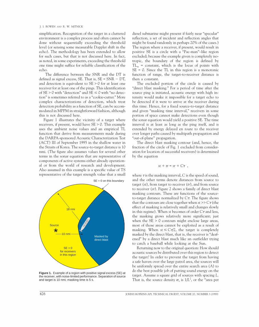
Figure 1 illustrates the vicinity of a target wherereceivers, if present, would have SE > 0. This exampleuses the ambient noise values and an empirical TLfunction that derive from measurements made duringthe DARPA-sponsored Acoustic Characterization Test(ACT) III of September 1995 in the shallow water inthe Straits of Korea. The source-to-target distance is 10nmi. (The figure also assumes values for several otherterms in the sonar equation that are representative ofcomponents of active systems either already operation-al or from the world of research and development.Also assumed in this example is a specific value of TSrepresentative of the target strength value that a small

18 nmi

10 nmi

Source

SE > 0for receiversin this region

Masked bydirect blast

SE = 0 on this boundary

Figure 1. Example of a region with positive signal excess (SE) atthe receiver, with noise-limited performance. Separation of sourceand target is 10 nmi; masking time is 5 s.

426 JOH

diesel submarine might present if fairly near “specular”reflection, a set of incident and reflection angles thatmight be found randomly in perhaps 20% of the cases.)The region where a receiver, if present, would result inpositive SE is a circle with a “Pac-man”–like regionexcluded; because the example given is completely iso-tropic, the boundary of the region is defined byTLtr = constant, which is the locus of points withSE = 0. Since the TL in this region is a monotonicfunction of range, the target-to-receiver distance isthen a constant.

The excluded portion of the circle is caused by“direct blast masking.” For a period of time after thesource ping is initiated, acoustic energy with high in-tensity would make it impossible for a target echo tobe detected if it were to arrive at the receiver duringthis time. Hence, for a fixed source-to-target distanceand given “masking time interval,” receivers in someportion of space cannot make detections even thoughthe sonar equation would yield a positive SE. The timeinterval is at least as long as the ping itself, and isextended by energy delayed en route to the receiverover longer paths caused by multipath propagation and“out-of-plane” propagation.

The direct blast masking contour (and, hence, thefraction of the circle of Fig. 1 excluded from consider-ation for location of successful receivers) is determinedby the equation

st 1 tr = sr 1 Ct ,

where t is the masking interval, C is the speed of sound,and the other terms denote distances from source totarget (st), from target to receiver (tr), and from sourceto receiver (sr). Figure 2 shows a family of direct blastmasking contours. These are functions of the source-to-target distance normalized by Ct. The figure showsthat the contours are close together when st >> Ct (theeffect of masking is relatively small and changes slowlyin this regime). When st becomes of order Ct and less,the masking grows relatively more significant; justwhen the SE > 0 contours might enclose large areas,most of those areas cannot be exploited as a result ofmasking. When st # Ct/2, the target is completelymasked by the direct blast, that is, the receiver is “deaf-ened” by a direct blast much like an outfielder tryingto catch a baseball while looking at the Sun.

Returning now to the original question: How shouldacoustic sources be distributed over this region to detectthe target? In order to prevent the target from havinga safe haven over the large patrol area, the sources willbe uniformly spread over the entire search area (A) todo the best possible job of putting sound energy on thetarget. Assume a square grid of sources with spacing L.That is, the source density ss is 1/L2, or the “area per

NS HOPKINS APL TECHNICAL DIGEST, VOLUME 20, NUMBER 3 (1999)

A MULTISTATIC PERFORMANCE PREDICTION METHODOLOGY

source,” defined as the inverse of density, is L2; hence,A/L2 sources would be spread over an area A. (Area persource is used here simply to denote the inverse ofsource density. It does not imply that target detectionis determined by only one of the sources dispersed inthe search area.) If the target moves very slowly withrespect to the “speed” at which adjacent source pingswill occur (v << L/t0, where t0 is the time betweenadjacent pings and v is the target speed of advance), onemay think of the target as (approximately) “frozen” inany “unit cell,” a square L on edge containing both asource (at its center) and the target at some heading(uniformly distributed) and at some location, alsouniformly distributed over this unit cell.

Now, for simplification, imagine that sources outsidethe unit cell containing the target are too distant tosignificantly contribute to detecting the target whencompared to the source in the unit cell, the closestsource. Consider the average area in which receivers (ifpresent) would have positive SE if the target headingwere such that TS exceeded the threshold TH; call thisAR(L;TH), the effective receiver area. This area can be

✸ ✸ ✸ ✸ TargetCτ/2s (2.0) s (1.5) s (1.0)s (0.8)

l = 0.6

l = 0.8

l = 1.0

l = 1.5

l = 2.0l = 5

l = 10

l = 50

CτScale

l = 0.51

l = 0.501

Figure 2. Direct blast masking contours. The source (s) is to the left of the target. Thedistances shown in parentheses are scaled with Ct. The source-to-target distances,denoted by l, are similarly scaled. Receivers to the right of the contours plotted are maskedby direct blast.

JOHNS HOPKINS APL TECHNICAL DIGEST, VOLUME 20, NUMBER 3 (1

found by averaging over target headings and locationsin the unit cell. To simplify the computation (we willremove this and some other simplifying assumptions inthe next section), assume that we can approximate thisarea by setting TS equal to TH and, at the same time,multiply by the probability that TS exceeds TH. Thus,

A L a l l dlL

R R/( ;TH) ( ;TH) ( ) prob(TS TH),= >∫ v

02 (1)

where l is the distance from the target to the source inthe center of the unit cell, and aR(l;TH) is the area withSE > 0 when TS = TH and source and target are sep-arated by l. That distance, l, ranges over the unit cell,with probability density function v(l), so that v(l)dl isthe probability that the source-to-target distance is be-tween l and (l 1 dl).

The receiver positions are totally unspecified, andthe target heading is statistically independent of itslocation (i.e., the target has no “map” of source loca-tions that allows it to use maneuvers to reduce TS tothe next ping). The probability that TS > TH can be

999)

calculated by considering the prob-ability that TS > TH for eachsource aspect angle, then averagingover source angles. That is,prob(TS > TH) is found directlyfrom the function of source and re-ceiver aspect angles TS (us, ur).

This prescribes how AR(L;TH)is calculated. The effective receiv-er area is clearly a function of thesystem parameters and the envi-ronment (which determine theterms in the sonar equation), andthe source density is implied in theintegration limits. An example ofAR is given in Fig. 3, where it isplotted against the area per source(L2) using the same TS threshold,TH, used in Fig. 1. Also plottedthere is integration over position,i.e., before reducing by the proba-bility that TS exceeds that thresh-old.

What is the relation of thisquantity to detection performance?If the density of receivers is sR andthe only source that would contrib-ute to detection of a target is thatwithin the unit cell, the expectednumber of receivers (nR) with pos-itive SE is sRAR. This is the ex-pected number of detections in asingle ping cycle, i.e., pinging

427

J. I. BOWEN AND R. W. MITNICK

around the field of sources once. That is, assuming thatonly the nearest source contributes to detecting thetarget (a not unreasonable assumption when TL is amonotonic function of st and the density of sources isnot too great) ensures that one need only be concernedwith the receivers “effective” from that ping in the unitcell containing the target.

Relating this single statistical measure, the expectednumber of detections, to the probability of detection(probability that at least one receiver gets contact,positive signal excess) requires an “invention.” Thereis no “correct” distribution function of contacts becausethe effective receiver area is a theoretical construct(because of the averaging), not an identifiable locus ofpositions. Even if it were a physical area, there is nospecified distribution of receivers, although reasonwould suggest that if the target is meandering over alarge area A the receivers should be regularly spread outover the search area. To proceed, imagine first thatthere is only one receiver. Since the unit cell with thetarget is anywhere in A, one expects the probability ofcontact to be AR/A and that of no contact in this pingcycle to be (1 2 AR/A). Since we are interested in largesearch areas, AR/A << 1, this is well approximated byexp(2AR/A). If there were several receivers Nspread over the search area, we would expect theprobability of no contacts to be simply the product,exp(2NAR/A). That is, the placement of a few receiv-ers over an area that is large compared with AR wouldsuggest that they are (very nearly, at least) statisticallyindependent. Since N/A is the density of receivers sR,then for a few receivers the probability of at least onedetection becomes 1 2 exp(2sRAR). We consequently

Figure 3. Example of effective receiver area AR plotted againstarea per source (L2) (single source, noise-limited performance).

1000

800

600

400

200

00 200 400 600 800 1000

Area per source (nmi2)

Effe

ctiv

e re

ceiv

er a

rea

(nm

i2 )

A AR R.prob(TS TH)= ≥' •

A a dL

R R/

( ;TH) ( )= ∫ l l lv0

2'

428 JO

assume that, to a good approximation, such a form willhold, and that the probability of success in one pingcycle, P1, is given by

P e A1 1= − 2sR R , (2)

as if the number of contacts had a Poisson distributionwith expected value nR = sRAR. If there are m pingcycles and they are statistically independent attemptsto detect the patrolling target, the probability becomes1 2 (1 2 P1)

m or

P emm A= −1 2 sR R . (3)

Equation 3 represents a response to the questionposed earlier under the many simplifying assumptionsstated: The probability of detection (occurrence of atleast one signal excess) in a “time” needed for m inde-pendent ping cycles is a simple function of the receiverdensity and AR, a construct that depends on the sourcedensity and all the physics and system parameters. Theindependence of ping cycles requires at least someminimum time interval between cycles, e.g., about 1 h,but specifically depends on the dynamics of the patrol-ling target and the decorrelation times of various phys-ical phenomena such as noise fluctuations. Note thatwhen the ping cycles are independent of one anotheras has been assumed, there is simply an inverse relationbetween the number (or density) of receivers and thenumber of ping cycles.

As a concrete illustration of an application, with thesame environment (Straits of Korea) used for Fig. 3 andthe same TS threshold, suppose that a number of re-ceivers are dispersed over 10,000 nmi2. Then Eq. 3permits one to estimate the number of sources (sourcepings per cycle) needed to attain a desired detectionprobability, say 0.9, in a prescribed number of pingcycles, for example m = 4 and m = 8. Results are givenin Table 1.

Table 1. Number of sources for probability 0.9 in10,000 nmi2.

Number ofreceivers 4 ping cycles 8 ping cycles

20 (many!) 2030 ≈60 1040 22 ≈450 14 (few)60 ≈8 (few)

HNS HOPKINS APL TECHNICAL DIGEST, VOLUME 20, NUMBER 3 (1999)

GENERALIZATIONSeveral assumptions identified in the foregoing sec-

tion were made for the sake of simplifying computationsand to illustrate the main ideas of MPPM. Some ofthese assumptions can be discarded; they are undulyrestrictive, and fairly complex computations do notchallenge contemporary personal computers. In partic-ular, the unnecessary assumptions are as follows:

1. The performance is determined by ambient noise, i.e.,reverberation plays no role.Comment: Reverberation is routinely predicted us-ing various well-established codes; such predictionsare readily incorporated in computing SE, hence inevaluating the areas with positive signal excess.

2. Contributions to the effective area come only fromthe source at the center of the unit cell containing thetarget in any ping cycle.Comment: All the sources spread about the searcharea may contribute to the area where receivers wouldhave positive signal excess. For every source (whetheror not it is in the unit cell containing the target), thearea of positive signal excess for potential receiversmay be computed for a specified target location in aunit cell and for a specified target heading, and theunion of areas (the logical “or”) can be computedonce the source locations are specified. For a homoge-neous environment, these locations will generallyfollow a regular grid, determined by the shape of thesearch area. As before, averaging over target positionsin the unit cell and headings would follow. Multiplesources may imply a great many computations. Onlya relatively small number of sources, however, usuallycontribute significantly to the effective receiver area.The other sources provide much less insonification ofthe target because they are too distant or are not atseparations that lead to large amounts of acousticenergy reaching the target (convergence zone separa-tions). Therefore, a bit of thought and precomputationwill provide practical guidance to the number ofsources to consider.

3. The calculation of SE, leading to evaluation of theeffective area, is for a fixed TS.Comment: As implied in the previous paragraph,once the source configuration is given, every targetheading determines the source and receiver aspectangles for each source ping and each potential re-ceiver location; hence, TS is determined by the TSfunction. Values of TS may be much greater than athreshold value over some small range of equivalentaspect angle. The choice of threshold value for TS issomewhat arbitrary, and when TS is much greaterthan the threshold value, the effective receiver areacontribution will be greater (perhaps much greater)than for the threshold value.

JOHNS HOPKINS APL TECHNICAL DIGEST, VOLUME 20, NUMBER 3 (

A MULTISTATIC PERFORMANCE PREDICTION METHODOLOGY

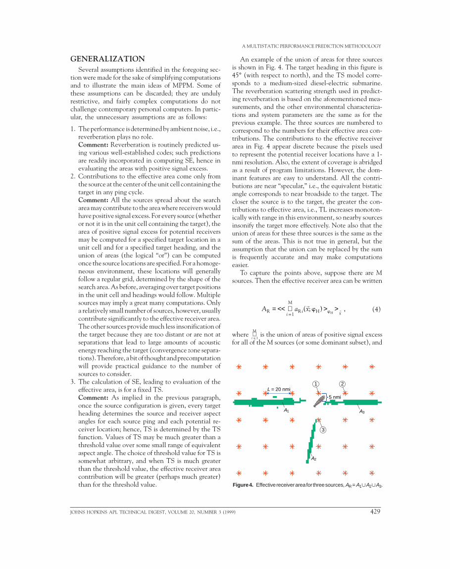
An example of the union of areas for three sourcesis shown in Fig. 4. The target heading in this figure is45° (with respect to north), and the TS model corre-sponds to a medium-sized diesel-electric submarine.The reverberation scattering strength used in predict-ing reverberation is based on the aforementioned mea-surements, and the other environmental characteriza-tions and system parameters are the same as for theprevious example. The three sources are numbered tocorrespond to the numbers for their effective area con-tributions. The contributions to the effective receiverarea in Fig. 4 appear discrete because the pixels usedto represent the potential receiver locations have a 1-nmi resolution. Also, the extent of coverage is abridgedas a result of program limitations. However, the dom-inant features are easy to understand. All the contri-butions are near “specular,” i.e., the equivalent bistaticangle corresponds to near broadside to the target. Thecloser the source is to the target, the greater the con-tributions to effective area, i.e., TL increases monoton-ically with range in this environment, so nearby sourcesinsonify the target more effectively. Note also that theunion of areas for these three sources is the same as thesum of the areas. This is not true in general, but theassumption that the union can be replaced by the sumis frequently accurate and may make computationseasier.

To capture the points above, suppose there are Msources. Then the effective receiver area can be written

A a xi =

M

i xR R H( ; ) ,H

= << ∪ > >→→

1w w (4)

where ∪i =

M

1 is the union of areas of positive signal excess

for all of the M sources (or some dominant subset), and

A1

5 nmi

L = 20 nmi1 2

3

A2

A3

Figure 4. Effective receiver area for three sources, AR = A1øA2øA3.

1999) 429

J. I. BOWEN AND R. W. MITNICK

wH denotes the target heading angle, a uniformly dis-tributed random variable. The angular brackets standfor averaging, first over target headings for fixed loca-tions x

→ then over the locations. Figure 5 shows the

effective receiver area (from Eq. 4) for nine sources.That is, M has been cut off at M = 9, the source in theunit cell containing the target plus 8 nearest sources ina square grid. Calculations were facilitated by choosingsample points for location, uniformly spread over theunit cell. Ten sample points were spaced over one-eighth of the unit cell, taking advantage of the inherentsymmetry in the source configuration. The distributionof target headings was also treated by sampling; in thiscalculation 15° steps were used. Figure 5 was computedby varying the source spacing L, i.e., the area per sourceis 1/L2.

With the revised, more general, version for comput-ing effective receiver area (that can be implemented ona PC for most propagation and reverberation and re-ceiver beam pattern codes), the relation to detectionperformance is, as before, given by Eq. 3.

EXAMPLESFor fixed (or desired or required) probability and

number of ping cycles, Eq. 3 shows a linear relationbetween the effective receiver area AR (an implicitfunction of area per source) and the area per receiver,the inverse of receiver density sR,

A m PmR R( / )ln[ / ( )] / .= − ⋅1 1 1 1 s

Therefore, many useful quantitative observations can bereadily inferred by plots such as those in Figs. 6 and 7.

Consider the sensitivity to the directivity index(DI), first by comparing curves of AR for different values

1000

800

600

400

200

01000

Area per source (nmi2)

Effe

ctiv

e re

ceiv

er a

rea

(nm

i2 )

1500500

Effective receiver area

Simplified AR

Figure 5. Example of effective receiver area plotted against areaper source (nine nearest-neighbor sources, reverberation included).

430 JOH

Area per source (nmi2)500 1000 15000

600

400

200

800

Area per receiver (nmi2)50010001500

P = 0.9in 4 pingcycles

20002000

DI = 5 dB

Reference:DI = 10 dB

DI = 15 dB

10 sources per10,000 nmi2

1000

1200

10 receivers per 10,000 nmi2

29

58

Effe

ctiv

e re

ceiv

er a

rea

(nm

i2 )

Figure 6. Sensitivity to directivity index (DI).

Area per source (nmi2)500 1000 15000

Area per receiver (nmi2)

50010001500

P = 0.9in 4 pingcycles

20002000

f0

f0 x 2

29Receivers per10,000 nmi2

Effe

ctiv

e re

ceiv

er a

rea

(nm

i2 )

168

100

200

300

Figure 7. Sensitivity to frequency f.

of DI. Figure 6 shows three such curves, one for DI =10 dB (“reference” value) and the others for DI = 5 and15 dB. For DI = 15 dB, AR is about 3 times as great asfor the reference value, while for DI = 5 dB it is abouthalf as large. This directly translates into the numberof receivers needed by a simple construction shown onthe figure: to reach probability 0.9 in 4 ping cycles inan area 10,000 nmi2 with 10 sources requires 29 receiv-ers for the reference case, 10 receivers if there is a 5-dB increase in DI, and 58 receivers if there is a 5-dBdecrease. This results primarily from the fact thatincreasing the DI leads to significant reduction inreverberation. For the portion of effective receiver areathat is dominated by reverberation (rather than ambi-ent noise), reducing reverberation translates directly torelaxing the TS requirements. The noise-dominatedportion of the effective receiver area is also enlarged byincreasing DI, causing effective regions to be found atgreater distances from the target.

NS HOPKINS APL TECHNICAL DIGEST, VOLUME 20, NUMBER 3 (1999)

For another example, consider that the (center)frequency f0 of the multistatic system is doubled to 2f0.As shown in Fig. 7, this causes a pronounced reductionin the effective receiver area. The reason lies in inputdata: In this environment, the so-called bottom scat-tering coefficient, for sound backscattered from thebottom, increases sharply with frequency. This is thedominant source of reverberation over the frequencyband of the impulsive sources used in the DARPAprogram. As indicated in Fig. 6, about 6 times as manyreceivers would be needed at the higher frequency(assuming, as in this calculation, no change in DI),despite the measured ambient noise being considerablyless at the higher frequency.

SUMMARYThe MPPM facilitates estimating the number of

sources and receivers needed to provide detection per-formance levels (probability) in time (number of pingcycles).

The core of MPPM is the effective receiver area.This is a construct obtained by calculating that areawithin which a receiver, if present, would detect asubmarine at a specified position and heading wheninsonified by sources uniformly spread over the searcharea, then suitably averaging over position and heading.

JOHNS HOPKINS APL TECHNICAL DIGEST, VOLUME 20, NUMBER 3 (19

A MULTISTATIC PERFORMANCE PREDICTION METHODOLOGY

The basic calculation in evaluating the effectivereceiver area is the active sonar equation. Hence, anycomputational technique that yields a SNR canbe used for this evaluation, such as those that do sowhen embedded within an operational Monte Carlosimulation.

Examples were presented to illustrate the concept,the calculations, and some applications of MPPM.These examples were for impulsive sources becauseDARPA’s interest in the methodology was stimulatedby measurements with simple impulsive sources. Themethodology is not limited to such sources; in partic-ular, it can be applied as well to Doppler-sensitivesources. Likewise, development of the methodology wasillustrated here using a detection model that results incontact if and only if SE > 0. The methodology also canbe applied to other detection models, in particular,letting the detection probability be determined by adistribution function, with the argument a function ofcomputed SNR.

ACKNOWLEDGMENTS: We thank Dr. William Carey, now at the NavalUndersea Warfare Center, for his interest, encouragement, and support; Carl A.Mauro of D. H. Wagner Associates, Inc., for adding the programs to SRAPS(Surveillance Resource Analysis and Planning Systems) that facilitate the effectivearea computations used in MPPM; and Tina M. Higgins of the APL InformationSystems and Technology Group for thoroughness and diligence in providing thecalculations used in the illustrative examples.

THE AUTHORS

JULIUS I. BOWEN is a Principal Professional Staff physicist in the InformationTechnology Group of the Submarine Technology Department, which he joinedin 1980. He has B.S. and M.S. degrees in physics from Syracuse University anda Ph.D. in physics from Catholic University. Before he came to APL, Dr. Bowenwas engaged in development at the Naval Ordnance Laboratory and incommunication theory research at the Bell Telephone Laboratories; he thenconducted and managed systems performance analysis at Raff Associates, Inc.,and ORI, Inc. At APL he has concentrated primarily on effectiveness analysisand predictions for underwater acoustic detection systems. His e-mail address isjulius.bowen@jhuapl.edu.

RONALD W. MITNICK is a member of APL’s Principal Professional Staff andthe Program Manager for Information Systems in the Maritime TechnologiesProgram Area of the Submarine Technology Department. He has a B.A. degreein physics from Yeshiva College. Before joining APL in 1991, he was a ProgramManager for the Naval Space and Warfare Systems Command, where he ledefforts to develop and field advanced undersea surveillance systems. At APL,he has concentrated primarily on concept development for advanced tacticalantisubmarine warfare and maritime surveillance. His e-mail address isron.mitnick@jhuapl.edu.

99) 431