a new method for efficient 3d reconstruction of outdoor ...eprints.lincoln.ac.uk/17744/7/17744...
TRANSCRIPT

A new Method for Efficient 3D Reconstruction of Outdoor
Environments Using Mobile Robots
Jaime A. Pulido Fentanes
Fundación CARTIF
Parque Tecnológico de Boecillo,
Valladolid,
España, 47151
Raul Feliz Alonso
Fundación CARTIF
Parque Tecnológico de Boecillo,
Valladolid,
España, 47151
Eduardo Zalama
Universidad de Valladolid,
ETSII,
Paseo del Cauce S/N,
Valladolid, España
Jaime Gómez García-Bermejo
Universidad de Valladolid,
ETSII,
Paseo del Cauce S/N,
Valladolid, España
Abstract
In this paper, a method for robotic exploration oriented to the automatic three-
dimensional reconstruction of outdoor scenes is presented. The proposed
algorithm focuses on optimizing the exploration process by maximizing map
quality, while reducing the amount of scans required to create a good quality 3D
model of the environment. This is done by using expected information gain,
expected model quality and trajectory cost estimation as criteria for view
planning. The method has been tested with an all-terrain mobile robot which is
also described in the paper. This robot is equipped with a Sick Lms 111 laser
scanner attached to a spinning turret, which performs quick and complete all-
around scans. Different experiments of autonomous 3D exploration show the
suitable performance of the proposed exploration algorithm.
1. Introduction
In emergency situations, it is often necessary to obtain as much information as possible about a
given area before planning and carrying out intervention actions. However, obtaining this
information is not an easy task, especially in the case of large outdoor environments where
access may be difficult and even unsafe for humans. In particular, 3D models represent a
powerful and desirable description of the environment. However, up to now, most 3D scanning
systems are of a stationary nature. This means that building a model of a large and complex
environment requires several scans taken separately and from many different viewpoints.

Unfortunately, setting up a typical stationary laser scanning system is a hard and time consuming
job, since scanners are often heavy and scanning work requires many auxiliary elements (tripod,
batteries, GPS antenna and computer) to be set up. Moreover, a human operator has to choose
which views will be less occluded and will provide the highest amount of new information, and
has to transport the whole system to the chosen location and set it up. The process is repeated
until the operator decides that the scans taken are enough to cover the whole area with the
desired quality. This decision is made using the operator’s experience, and a close look at the
resulting model is not taken until all the captured data is processed and aligned at a later step,
often not in field. Then, if a portion of the environment has been missed, or the resulting model
quality was not good enough, the scanning system has to be redeployed. This manual procedure
is a big liability in emergency and disaster situations, where quickly obtained 3D models of the
environment are vital to planning rescue operations. However, the main drawback for SSRR
scenarios is the presence of the human operator in an environment which can be unsafe for
his/her health (presence of toxic gases, fire, radioactivity and biological threats).
The use of mobile robots equipped with on-board 3D scanning systems emerges as a suitable
alternative (Blaer & Allen, 2007) (Nüchter, Lingemann, Hertzberg, & Surmann, 2007), given
that robots provide mobility, computing resources, localization systems and physical support to
the scanning equipment. However, though the use of mobile robots can largely reduce the
scanning process effort, the automation of the view selection process is still an open problem.
This issue has been addressed within the field of mobile robot exploration. However, most of the
research effort has focused on the SLAM problem, so proposed techniques are designed to
improve the extraction of relevant features along robot trajectories in order to provide robot
localization and map information. Moreover, the main objective of these approaches is often to
autonomously obtain indoor maps which help robots to self localise, and the mapping process is
constrained to flat environments.
Outdoor environments have many characteristics that make the problem different from indoor
scenarios. The environment is less structured: it is not limited by walls, the floor is not flat, there
are arbitrary but relevant 3D elements (such as trees, stones and cars) and thus, mere 2D maps
are not efficient for navigation. Moreover, 3D mapping becomes a complex problem due to the
huge memory and computational resources required for data handling, besides other problems
such as occlusions. Fortunately, the localization problem may be less severe in outdoor
environments due to the availability of absolute localization sensors such as DGPS and
compasses, which provide reasonably accurate robot localization.
In this context, the method presented in the present paper is focused on optimizing the
exploration process by maximizing map quality, while reducing the amount of scans required to
create a good quality 3D model of the environment. The goal is to obtain a robot that can
efficiently build a model of its surrounding environment. The robot takes previous data into
consideration in order to choose the best next locations to do a new scan, and computes the
trajectory towards these locations. This methodology can be applied to most outdoor scenarios
such as urban locations, monuments, archaeological sites and forests.
In the present paper, the robotic platform used to set up our method is first presented; then the
algorithm for view planning is explained; and finally, results and conclusions are given.

2. Related Work
3D mapping on the field of Safety, Security and Rescue Robotics (SSRR) has been thoroughly
studied and proven to be very useful in these situations. For example in (Ohno, Tadokoro,
Nagatani, Koyanagi, & Yoshida, 2009) the authors developed a method to create a 3D map of an
underground mall and subway station using odometry and an offline 3D scan matching method
based on ICP and an additional gravitation constraint that was tested in a simulation of a terrorist
attack. Another remarkable example is (Pathak, Birk, Vaskevicius, Pfingsthorn, Schwertfeger, &
Poppinga, 2010), where a method for 3D mapping based on pose-graph relaxation was
developed and tested on different SSRR scenarios such as a collapsed car park and a flooding
disaster. There are currently different projects oriented to creating methods for modelling
outdoor structures. Most of these projects are intended for building large scale 3D models of
cities and focus mainly on the data processing and fusion processes, rather than on the view
planning problem. Some remarkable projects are the 3-D city model construction project at
Berkeley (Früh & Zakhor, 2003), the MIT City Scanning Project (Teller, 1997), the 4D Cities
project at Georgia Tech (Dellaert, 2005) and Google Street View (Williams, 2010). In these
projects, data processing is completed after the capture stage, so this phase is not automated.
Some other projects address 3D data processing during the capturing stage. Smarter Team
(Jensen, Weingarten, Kolski, & Siegwart, 2005) and (Pfaff, Triebel, Stachniss, Lamon, Burgard,
& Siegwart, 2007) is an example, where an effort to build an autonomous car is carried out in
order to demonstrate fully autonomous navigation and 3D mapping in outdoor environments. In
this case, a 3D data processing module is required for finding traversable areas in the
environment. However, a human operator has to choose the waypoints that the robot has to
follow, so the exploration of the environment is left to a human component.
(Nüchter, Lingemann, & Hertzberg, 2006) applied the concept of SPLAM to outdoor 3D
mapping and navigation. Under this concept, a mobile robot designed for outdoor scenarios
would have to take a scan, align it with previous scans, extract drivable surfaces within the
environment and then use this information to plan the next observation position. Unfortunately,
the planning stage was not covered by this work.
On the other hand, several different exploration techniques have been proposed using 2D data
within the field of robotic exploration for planar scenarios. Two main strategies are followed:
strategies where a predefined behaviour is selected (such as wall following or moving to random
positions) based on a priori information of the environment (Danner & Kavraki, 2000), (Bourque
& Dudek, 1998), and strategies that predict which movement will most improve the robots’
knowledge of the environment, using previously acquired information.
The first group of strategies lacks adaptability to unknown environments, where they tend to
either leave unexplored areas or be highly inefficient. The second group of strategies has
received more attention, since they use information from the environment to decide further
actions; they are more adaptable to any kind of environment. In general, all these methods are
known as next best view (nbv), given that their main focus consists in finding the next best
observation position to make the exploration process efficient.
Common methods within nbv approaches are greedy methods (Tovey & Koenig, 2003), where
the robot moves to the closest location of interest; frontier based methods (Yamauchi, 1997),
where candidate locations are generated on the frontier between the explored and unexplored
areas of the environment; and information based strategies, which use evaluation functions

where different criteria can be used to choose the next best position according to the selected
criteria, for example travelling cost (Yamauchi, Schultz, Adams, & Graves, 1998).
Among the information based methods, some use functions to predict the utility of a location.
For example, the utility of a target location is defined as an expected information gain in
(Newman, Bosse, & Leonard, 2003), and travelling cost is combined with information gain in
(Gonzalez-Baños & Latombe, 2002), so that the next best view point is chosen to maximize
coverage and reduce travelling distance.
Some strategies find interest areas within the map that are also used as criteria. For example, in
(Grabowski, Khosla, & Choset, 2003), relevant features within the map are included and used for
evaluating the next best view, considering that seeing these regions will facilitate SLAM. These
strategies are known as active SLAM strategies. However, all these methods were proposed for
planar environments represented by a 2D map.
A different solution for outdoor 3D exploration is proposed in (Blaer & Allen, 2009) . It works in
two stages. In the first stage, a 2D floor map of the area that has to be scanned is used to find
possible occlusions that a 3D scan would have from different floor points. The combination of
viewpoints that requires the lowest number of scans to entirely cover the target area is then found
with this process. Once a 3D scan has been done from each previously calculated viewpoint, a
second view planning algorithm step is then used to cover all unpredicted occlusions on the
model with as few scans as possible. However, in this latter work, a priori information of the
environment is required; the method proposed here only uses information captured by the robotic
system at the exploration time and, from that information, chooses the next best viewpoint for
3D reconstruction.
3. Our 3D Reconstruction Process
There are multiple methods for creating 3D models of outdoor environments, as discussed in the
previous section. The focus of the present work is to analyse 3D data in order to improve the data
acquisition process. We have developed a mobile robot equipped with a 3D scanner on a
spinning turret that can take 3D scans from different viewpoints. Scans are taken at stationary
robot locations, which eases data processing (for example, surface reconstruction through point
triangulation) and allows higher 3D resolution to be reached.
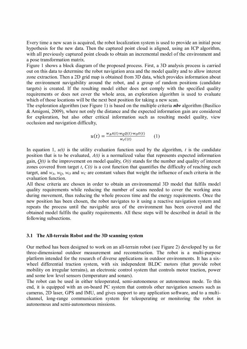
Figure 1- Block diagram of the 3D reconstruction process (left). Diagram of the exploration algorithm (right).
Every time a new scan is acquired, the robot localization system is used to provide an initial pose
hypothesis for the new data. Then the captured point cloud is aligned, using an ICP algorithm,
with all previously captured point clouds to obtain an incremental model of the environment and
a pose transformation matrix.
Figure 1 shows a block diagram of the proposed process. First, a 3D analysis process is carried
out on this data to determine the robot navigation area and the model quality and to allow interest
zone extraction. Then a 2D grid map is obtained from 3D data, which provides information about
the environment navigability around the robot, and a group of random positions (candidate
targets) is created. If the resulting model either does not comply with the specified quality
requirements or does not cover the whole area, an exploration algorithm is used to evaluate
which of those locations will be the next best position for taking a new scan.
The exploration algorithm (see Figure 1) is based on the multiple criteria nbv algorithm (Basilico
& Amigoni, 2009), where not only the distance and the expected information gain are considered
for exploration, but also other critical information such as resulting model quality, view
occlusion and navigation difficulty,
(1)
In equation 1, u(t) is the utility evaluation function used by the algorithm, t is the candidate
position that is to be evaluated, A(t) is a normalized value that represents expected information
gain, Q(t) is the improvement on model quality, O(t) stands for the number and quality of interest
zones covered from target t, C(t) is a cost function that quantifies the difficulty of reaching each
target, and wA, wQ, wO and wC are constant values that weight the influence of each criteria in the
evaluation function.
All these criteria are chosen in order to obtain an environmental 3D model that fulfils model
quality requirements while reducing the number of scans needed to cover the working area
during movement, thus reducing the whole process time and the energy requirements. Once the
new position has been chosen, the robot navigates to it using a reactive navigation system and
repeats the process until the navigable area of the environment has been covered and the
obtained model fulfils the quality requirements. All these steps will be described in detail in the
following subsections.
3.1 The All-terrain Robot and the 3D scanning system
Our method has been designed to work on an all-terrain robot (see Figure 2) developed by us for
three-dimensional outdoor measurement and reconstruction. The robot is a multi-purpose
platform intended for the research of diverse applications in outdoor environments. It has a six-
wheel differential traction system, with six independent BLDC motors (that provide robot
mobility on irregular terrains), an electronic control system that controls motor traction, power
and some low level sensors (temperature and sonars).
The robot can be used in either teleoperated, semi-autonomous or autonomous mode. To this
end, it is equipped with an on-board PC system that controls other navigation sensors such as
cameras, 2D laser, GPS and IMU, and gives support to any application software, and to a multi-
channel, long-range communication system for teleoperating or monitoring the robot in
autonomous and semi-autonomous missions.
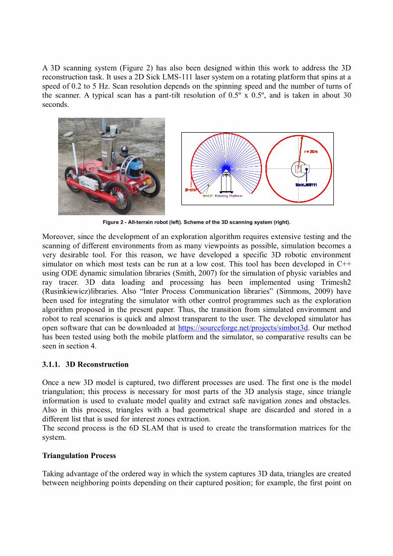
A 3D scanning system (Figure 2) has also been designed within this work to address the 3D
reconstruction task. It uses a 2D Sick LMS-111 laser system on a rotating platform that spins at a
speed of 0.2 to 5 Hz. Scan resolution depends on the spinning speed and the number of turns of
the scanner. A typical scan has a pant-tilt resolution of 0.5º x 0.5º, and is taken in about 30
seconds.
Figure 2 - All-terrain robot (left). Scheme of the 3D scanning system (right).
Moreover, since the development of an exploration algorithm requires extensive testing and the
scanning of different environments from as many viewpoints as possible, simulation becomes a
very desirable tool. For this reason, we have developed a specific 3D robotic environment
simulator on which most tests can be run at a low cost. This tool has been developed in C++
using ODE dynamic simulation libraries (Smith, 2007) for the simulation of physic variables and
ray tracer. 3D data loading and processing has been implemented using Trimesh2
(Rusinkiewicz)libraries. Also “Inter Process Communication libraries” (Simmons, 2009) have
been used for integrating the simulator with other control programmes such as the exploration
algorithm proposed in the present paper. Thus, the transition from simulated environment and
robot to real scenarios is quick and almost transparent to the user. The developed simulator has
open software that can be downloaded at https://sourceforge.net/projects/simbot3d. Our method
has been tested using both the mobile platform and the simulator, so comparative results can be
seen in section 4.
3.1.1. 3D Reconstruction
Once a new 3D model is captured, two different processes are used. The first one is the model
triangulation; this process is necessary for most parts of the 3D analysis stage, since triangle
information is used to evaluate model quality and extract safe navigation zones and obstacles.
Also in this process, triangles with a bad geometrical shape are discarded and stored in a
different list that is used for interest zones extraction.
The second process is the 6D SLAM that is used to create the transformation matrices for the
system.
Triangulation Process
Taking advantage of the ordered way in which the system captures 3D data, triangles are created
between neighboring points depending on their captured position; for example, the first point on

a laser reading makes a triangle with the second point of that reading and the first point of the
next reading. If a ray is over the maximal scanner reach the triangle is not created.
Once every triangle has been created every triangle is evaluated separately using the law of sines
for relating the length of the sides of each triangle to the sines of its angles. If this relation is not
within certain values (γmin and γmax) the triangle is discarded (see Figure 3).
Figure 3 - Triangle Discard Methodology
Triangulation is done online with the 3D data capture process, the triangle discarding process
takes less than 10 milliseconds after the data capture process is completed.
6D SLAM
Following the 6D SLAM process presented by (Nüchter, Lingemann, Hertzberg, & Surmann,
2007), we execute an ICP algorithm to align the last captured point cloud with its closest points
clouds, giving it an initial pose estimation that is given by the robot’s localization system. When
a new loop closure is detected, a back propagation algorithm is run to realign the whole model.
The model alignment process is the following:
1. Estimate robot position and orientation, using robot localization system.
2. Use these estimations to create an initial transformation matrix for the ICP alignment.
3. Align the scans using ICP.
4. If a loop closure is detected, back-propagate the error to previous registered scans.
Each alignment done with the ICP algorithm takes around 7 seconds. The back propagation
algorithm runs only when a new loop closure is detected and needs 5 seconds per scan.
3.2 3D Data Analysis
In this stage, the acquired 3D mesh is analyzed point by point to extract which points correspond
to traversable surfaces and obstacles, to estimate model quality at each point and to extract
interest zones from discarded triangles. This process is executed at every robot scan.
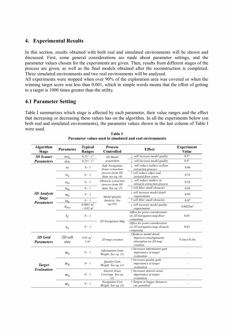
3.2.1 Extraction of safe navigation zones and obstacles
3D data contains a large amount of information about the environment, and 3D points can
correspond to obstacles, drivable surfaces (ground) or objects that the robot cannot reach
(Nüchter, Lingemann, & Hertzberg, 2006). The extraction of safe navigation areas is done by
calculating the probability of each mesh point belonging to the ground (safe navigation zones) or
to an obstacle. This data is useful to analyze navigability within the surrounding area.
If a point is at a reachable angle for the robot (i.e. the robot does not need to climb beyond its
possibilities to reach this point), and its normal vector projection onto the world Z axis is large
enough, this point has a high probability of belonging to a traversable zone from a local point of
view.
However, neighboring points also have to be considered. For example, a point on an elevated
plane may comply with local conditions, but its neighbor’s probabilities could be much lower, so
it should not be considered a safe navigation point. For this reason, the extraction of safe
navigation areas is done in two steps. First, a probability from a local point of view Fpl(p) is
computed using (2), where Pz is the point height from the robot base, dp is its distance to the
scanner on the XY plane, Nz is its normal Z component on the global reference system and Θ
(see Figure 4) is the maximum angle that the robot can climb.
(2)
Figure 4 - Probabilities of belonging to a surface from point angle and distance
Then, a probability from a “global” point of view Fpg(p) is computed as the average of each
neighbouring point probability, Fpl(p) (points sharing 3D mesh triangles with point p),
(3)
Where γ(p) is the set of neighbours of point p and n is the number of neighbours. Once Fpg(p) has
been computed, the final probability F(p) for each point is obtained by weighting their
corresponding probabilities with wl and wg,
(4)

A point can belong to an obstacle if it is at a reachable position for the robot and the plane to
which it belongs is facing the robot (the dot product between the ray and the point normal vector
is close to 1). Neighbours are also relevant since an obstacle point surrounded by floor points can
be traversable. The probability of belonging to an obstacle is computed using a “local”
probability function Bl(p) (5) and a “global” probability function Bg(p) (6):
(5)
(6)
where |Nxy| is the magnitude of the resulting vector addition of point normal components on the
X and Y axis, is a vector from the 3D scanner to point p and is its normal vector. In (6), the
neighbours to point p are used to find the global probability value. Then, the final probability
B(p) is obtained by weighting the Bl(p) and Bg(p) relevance with wbl and wbg,
(7)
Ground and obstacle probability values are used to create a navigation map that can be used to
find trajectories and calculate route difficulty, as will be explained in section 3.3. All the results
of this process will be shown in section 4.
3.2.2 Model quality analysis
Model quality has to be analyzed point by point because it is not a homogeneous characteristic
and is affected by various factors within one scan. In the analysis process, each point p gets a
score AP(p) (between 0 and 1) where 0 corresponds to bad quality and 1 to the desired quality or
better. In this case Model quality is measured using point area and ray incidence angle as criteria.
These criteria were chosen because they can be calculated in a quick and simple way, and they
give a good idea of the resulting quality of the mesh, due to the fact that they provide
information on the resolution of the scan at each point and how trustworthy the information
provided by each point is. This score is calculated using the following equations:
(8)
where AA(p) is a function that compares the current area per point against the maximum desired
area for point p, where PAr is a point p area which is easily computed by adding one third of the
area of each triangle that point p belongs to. Amax is the maximum desired point area and is a
parameter given to the algorithm that depends on desired scan resolution and maximum distance
to an object at scanning.
(9)

AIp(p) is a quality factor that depends on the ray incidence angle for the point's plane, is a
vector from the 3D scanner to point p and is its normal vector.
(10)
AP(p) is the final score for each point, where and weight the relevance of the area against
the ray incidence angle. Usually, is higher than , since point area is the most relevant
factor, and only really low scores on the ray incidence quality should affect the overall score.
Figure 5 shows an example of the quality analysis process on a simple simulated environment
using both criteria.
Figure 5 - quality score using point area (left); quality score by ray incidence angle (right). Colder colours indicate higher quality scores.
3.3 Candidate Target Evaluation
Candidate evaluation using 3D data can be a really time consuming process that also needs a
great amount of resources. For this reason, a 2D information grid is used in this work to keep
time and resources low without losing information from 3D data. Each cell in this grid stores all
the information from an area of the environment, so processing information becomes much
simpler. All the information of a mesh is projected onto this grid every time a new scan is taken.
The resulting representation is useful for many different tasks, such as computing navigation
maps by analyzing the amount of points that have a high probability of belonging to obstacles, or
traversable surfaces in a cell.
3.3.1 Extraction of interest zones
Interest zones are extracted from models’ discarded triangles, which are usually occluded planes.
A vector pointing to the centre of each discarded triangle is created. These vectors are stored on a

list, and are used to measure how well interest zones will be scanned from each candidate
position. The resulting list is projected onto a 2D representation where information on which
occlusion planes are covered from each evaluated target t, can be extracted using
(11)
where δ is the set of visible cells from target t, β is the set of interest zones stored for each cell j,
is a vector from the 3D scanner to the point that marks the centre of an interest zone and is
the vector that is normal to the occlusion plane. Interest zones extracted from a simple simulated
environment are shown in Figure 6.
Figure 6 - Zones of Interest extracted from a simple environment.
3.3.2 2D navigation map
This representation is based on the navigability concept (Hertzberg, Lingemann, Christopher,
Nüchter, & Stiene, 2008). It is a map very similar in appearance to the occupancy grid maps used
for 2D environments. However, cells in occupancy maps contain the probability of a cell being
occupied by an object, while cells in the navigation map contain the probability of a cell being
traversable by the robot.
Each time a new point with a high probability of belonging to a traversable surface is added to a
cell, the probability of this cell being traversable increases. Otherwise, if an obstacle point is
added, then this probability decreases. Navigability per cell ranges from 0 to 1, where 1
corresponds to a completely traversable cell. This map is computed using all points that have a
probability of belonging to a traversable surface over a given value, or a probability of
belonging to an obstacle over a value.
(12)

(13)
(14)
(15)
In this expression, φ is the set of points on cell c with , npf is the number of points in
the set φ, ∝ is the set of cell points with and npo is the number of points in the group
∝. Candidate targets are generated in cells where , so every evaluated target is
reachable. Targets are distributed uniformly around the robot’s position; so many different
viewpoints are evaluated.
3.3.3 Expected information gain
The amount of new information that can be acquired from each evaluated candidate is computed
upon the number of points and the minimum and maximum point heights per cell. This data is
used to compute how many new cells will be scanned from a given target and which cells will be
occluded by other ones.
In concrete, the first relevant value is the area covered from each candidate target An(t), which is
obtained using:
(16)
where Ac is the area represented by each cell and Cse is the number of unexplored cells within
the scanner range. Computation is refined by subtracting the area of occluded cells Ao(t) from the
unexplored area that could be covered from a given candidate target.
Occluded cells are computed using a height map that is created using per cell min and max point
heights; as well as using the information of the closest explored cell in the robot direction for
unexplored cells.
Three points mk are generated at each cell: one point at the minimum height of 3D points
corresponding to this cell, another one at the maximum height that the scanner could reach on
that cell from the evaluated target, and a third one at the middle of the said points. Then, rays are
traced from the scanner position at the evaluated target t, to these three points, and lines that
cross a cell under its maximum height nil are counted up. The occluded area is then computed
using
(17)
Finally, the expected information gain, A(t), is obtained upon (16) and (17) using
(18)
3.3.4 Expected model quality improvement
Model quality gain is the difference between quality information stored in the 2D information
map and the quality information after a scan is taken from the evaluated target t.
Expected quality is calculated using two terms. The first one is the expected per cell point area
EQAP, which is computed using the distance from the candidate target to each cell re, the
maximum desired point area Amax and Pan-Tilt resolutions resp and rest.

(19)
(20)
The second term corresponds to the quality improvement computed from the laser incidence
angle. A new ray incidence quality for each point on the cells within the scanner reach range
from the evaluated target, EIC(c), is computed using:
(21)
where φ is the set of points stored in each cell, npc is the number of points in each cell, is a
vector from the evaluated target to each cell point and is a unit vector normal direction to each
cell point. Expected quality gain Q(t) is obtained using:
(22)
where σ is the set of cells within the range of the scanner, AP(p) is the quality per point mark
computed in section 3.2.2, and and are the values introduced in that section.
3.3.5 Trajectory cost evaluation
Trajectory cost evaluation is done by adding the difficulty of crossing each cell on the trajectory.
This difficulty depends on the slope of each cell, the difference between the entry and the exit
angle for each cell, the navigability value computed in section 3.3.2 and the distance
between cells dec. Trajectory cost is computed using:
(23)
where fga is a difficulty scale factor that depends on the trajectory curvature (see Figure 7), ci is
the current cell in the trajectory and Θmax is the maximum slope that the robot can climb.
Figure 7 - Difficulty factor when crossing Cells (Left); Difficulty Map upon Slope (right).
4. Experimental Results
In this section, results obtained with both real and simulated environments will be shown and
discussed. First, some general considerations are made about parameter settings, and the
parameter values chosen for the experiments are given. Then, results from different stages of the
process are given, as well as the final models obtained after the reconstruction is completed.
Three simulated environments and two real environments will be analysed.
All experiments were stopped when over 90% of the exploration area was covered or when the
winning target score was less than 0.001, which in simple words means that the effort of getting
to a target is 1000 times greater than the utility.
4.1 Parameter Setting
Table I summarizes which stage is affected by each parameter, their value ranges and the effect
that increasing or decreasing these values has on the algorithm. In all the experiments below (on
both real and simulated environments), the parameter values shown in the last column of Table I
were used. Table I
Parameter values used in simulated and real environments
Algorithm
Stage Parameter
Typical
Ranges
Process
Controlled Effect
Experiment
Value
3D Scaner
Parameters
resp 0.25º - 1º 3D Model
acquisition
↓ will increase model quality 0.5º
rest 0.25º - 1º ↓ will increase model quality 0.5º
3D Analysis
Stage
Parameters
wl 0 - 1 Safe Navigation
Zones extraction
process from 3D
data. see eq. (4)
↓ will reduce outliers in floor
extraction process 0.66
wg 0 – 1 ↑ will reduce edges and
isolated floor zones 0.33
wbl 0 – 1 Obstacle extraction
process from 3D
data. See eq. (7)
↓ will reduce outliers in
obstacle extraction process 0.55
wbg 0 – 1 ↑ will filter small obstacles 0.45
0 – 1 Model Quality
Analysis. See
eq.(10)
↓ will increase model detail
requirements 0.93
0 – 1 ↑ will filter small obstacles 0.07
Amax 0.0001 m2
– 0.02 m2
↓ will increase model quality
requirements 0.0025m
2
0 – 1
2D Navigation Map
Offset for point consideration
on 2D navigation map floor
computing
0.65
0 – 1
Offset for point consideration
on 2D navigation map obstacle
computing
0.83
2D Grid
Parameters
2D cell
size 0.01 m2–
1 m2 2D map creation
↑Reduces model detail,
Improves misalignments
absorption on 2D map
creation.
0.3m x 0.3m
Target
Evaluation
0 – 1 Information Gain
Weight. See eq. (1)
↑ Increases information gain
importance at target
evaluation
-
0 – 1 Quality Gain
Weight. See eq. (1)
↑ Increases quality gain
importance at target
evaluation
-
0 – 1
Interest Areas
Coverage. See eq.
(1)
↑ Increases interest areas
importance at target
evaluation
-
0 – 1 Navigation Cost
Weight. See eq. (1)
↑ Targets at bigger distances
are punished -
Please note that the parameters in equation 1 are not presented in the last column, given that they
have been tuned separately for each experiment, in order to test specifically how they affect the
behaviour of the algorithm.
Other Considerations for Parameter Tuning
For floor extraction, a higher wl value leads to better results. Moreover, wl and wg should be set
to 1, unless most points want to be considered as floor ones. In this case, these values could be
larger than 1. On the contrary, values under 1 could be suitable when most points in the floor
should not be considered. Once the desired floor extraction behaviour has been obtained, the
values of these parameters can remain constant during the whole exploration process. For the 2D
Navigation map, and values behave as offsets in order to consider only those points over a
specific score when creating the map.
Model quality analysis is done in equation (10). The Amax value involved in this equation
(through AA(p) parameter) is the desired 3D model resolution. A suitable value for Amax can be
calculated by providing the ideal distance to objects (dobj) and the angular resolution of scan (resp
and rest), by means of:
(24)
The most relevant parameters are those for target evaluation (equation (1)). These parameters
affect the behaviour of the algorithm. In concrete, wA, wQ and wO can be given values between 0
and 1, proportionally to the desired influence of the corresponding term. However, a value of
over 0.25 is not recommended since it might lead the system to behave unexpectedly.
Finally, the wc parameter can be computed as the inverse of the minimum desired distance to the
next target on plane environments (e.g. 0.2 value for targets at a distance of at least 5 meters).
4.2 Simulated Environments
We have tested our method in three different simulated environments. The first one is a simple
environment with only one building and a tree, placed on an irregular hill-shaped terrain. This
environment has been used for evaluating how the different parameter values affect the
behaviour of the algorithm, and how slopes may affect the navigability analysis and the
trajectory cost estimation. The other two environments are more complex. The second one is a
structured urban environment, intended for testing how the robot would move in an environment
where navigation complexity is not high and the system can freely move along many different
trajectories. The last simulated environment is the most complex. It is a cluttered outdoor
scenario where only some paths are safe for the robot, so navigation complexity is high. The
objective was to see if the algorithm can choose targets that are safe, and can efficiently manage
cluttered environments.

4.2.1. Simple Environment
Figure 8 – Screenshot of the simple environment. The exploration area is squared in red.
Three experiments were carried out in this environment (Figure 8), using three different value
choices for parameters in (1) in order to achieve different objectives. In the first experiment, the
parameters were set in a balanced way; in the second experiment, information gain was given
more importance than the other parameters, and in the third experiment, model quality was the
dominant criterion. The chosen parameters can be seen in Table II.
Table II
Parameters Used In The Experiments
wA wQ wO wC
Experim. I 0.43 0.35 0.22 0.09
Experim. II 0.65 0.25 0.10 0.09
Experim. III 0.36 0.5 0.14 0.09
The wc parameter was not modified, so trajectories are determined only by the desired model
criteria. Resulting trajectories can be seen in Figure 9.
Figure 9 - Resulting trajectories for Experiment I (left); Experiment II (centre); Experiment III (right). Colder Colours Represent
Better Quality
A fourth experiment with an implementation of a greedy mapping algorithm was carried out for
comparison. In this experiment the system goes to the position where the estimation of
information gain is the highest. The resulting trajectory is shown in Figure 10.

Figure 10 - Resulting trajectory for greedy mapping algorithm. Colder Colours Represent Better Quality
Table III shows the result for each experiment in terms of travelled distance, the number of
scans, the amount of cells explored within the given area and a quality score computed by the
averaging of the per-point quality score on each environment cell.
Table III
Results Obtained In Experiments Travel
Distance
Quality
Score Coverage Scans
Exp. I 106 m 0.6846 92.5 % 12
Exp. II 107 m 0.6904 94.1 % 10
Exp. III 128 m 0.7503 93.6 % 13
Greedy 116 m 0.5013 91.4 % 8
From these results, it can be seen that experiment II proved to be the most efficient solution,
since it covered the entire area using only ten scans, whilst travelling only 1 meter more than the
shortest trajectory. Experiment I led to a very similar model, but extra scans were required.
Finally, experiment III required 13 scans to cover the whole area; however it led to a very high
quality model. In comparison with the greedy mapping algorithm, the proposed algorithm may
require more scans to achieve the same level of coverage. However, it provides a much higher
quality score. The difference in terms of travelled distance and coverage is not noticeable, but the
trajectory is inefficient for the greedy method since it requires the robot to execute rougher turns
to reach the targets. Finally, there is an important difference in the quality distribution, as it is
much more even in the experiments carried out with the proposed algorithm. Figure 11shows the
simulated environment and a screenshot of the reconstructed model.
Figure 11 - Screenshot of the reconstructed model.
4.2.2. Structured Environment
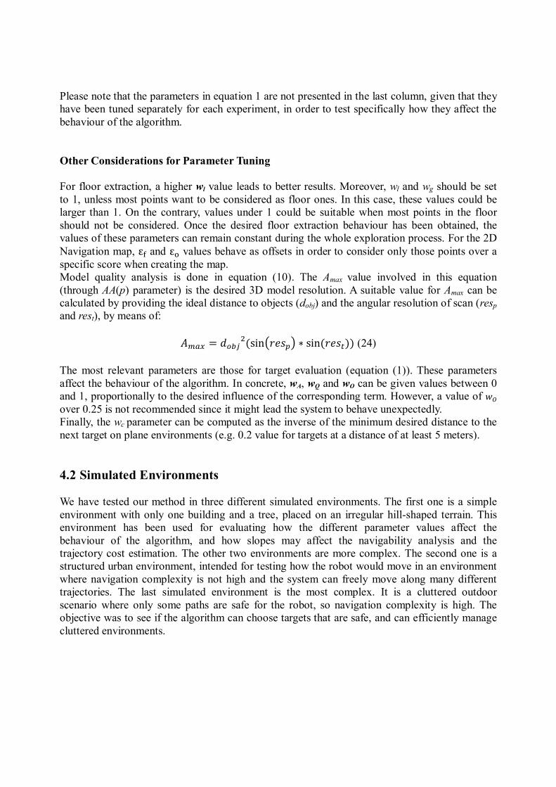
Figure 12 - Simulated structured environment
Figure 12 shows the simulated structured environment. Two experiments were carried out on this
environment following two different strategies. In the first experiment, interest zones and map
quality were chosen as the dominating criteria; in the second experiment, information gain was
the dominating criterion and navigation cost weight was also slightly lower. Table IV shows the
selected parameter values.
Table IV
Parameters Used In The Experiments
wA wQ wO wC
Exp. I 0.2 0.55 0.25 0.09
Exp. II 0.65 0.25 0.10 0.09
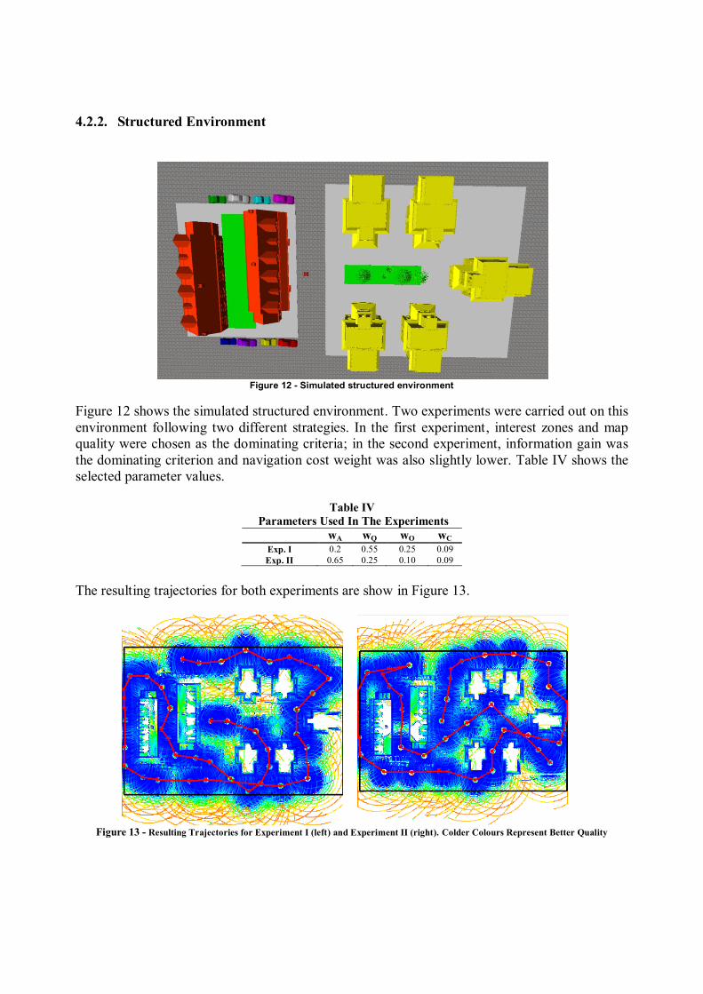
The resulting trajectories for both experiments are show in Figure 13.
Figure 13 - Resulting Trajectories for Experiment I (left) and Experiment II (right). Colder Colours Represent Better Quality
Table V shows the result for both experiments in terms of travelled distance, the number of scans
done in each experiment, the amount of cells explored within the given area and the quality score
defined in the previous subsection.
Table V
Results Obtained In Experiments Travel
Distance
Quality
Score Coverage Scans
Exp. I 352 m 0.6813 95 % 43
Exp. II 397 m 0.726 94.8 % 39
From these results, it can be seen that the algorithm can be used efficiently on structured
environments. Also, it can be noted that both strategies are useful and have similar results, the
difference in terms of coverage and quality scores is very small, and the longest trajectory
travelled by experiment II is compensated by a smaller number of scans. It is important to
mention that, due to the difference in target evaluation weight, both trajectories started out in
very different ways. However, both experiments had very similar results, which may be because
of the highly structured environment designed for the test, since interest zones and quality gain
have very similar scores on targets all over the map, so information gain became the dominant
criterion in both cases. Experiments in a cluttered environment will show that this happens only
on structured scenarios.
Figure 14 shows the 2D navigation map and the final reconstructed model for experiment II.
Figure 14 - Navigability map (left) and 3D reconstruction (right) for Experiment II
4.2.3. Cluttered Environment
A cluttered environment can be seen in Figure 15. It can be seen that the terrain has few safe
paths and navigation complexity is very high. The environment is designed in such a way that
the robot has to cross under and over bridges (in gray, in the figure) so that the ability of the
system to manage gaps and overhanging structures can be tested.
The starting position is on the upper right corner of the environment, and the robot has to find
suitable paths to cover the whole environment. The objective of this experiment was to test if the
algorithm would choose targets that are safe and can efficiently manage cluttered environments.
Two experiments were carried out on this environment, Experiment I with a very high navigation
cost and balanced parameter for exploration, and another one (Experiment II) with a lower

navigation cost and a higher weight for the information gain parameter. Table VI shows the
parameters used in both experiments.
Table VI
Parameters Used In The Experiments
wA wQ wO wC
Exp. I 0.40 0.35 0.25 0.125
Exp. II 0.65 0.3 0.05 0.08
Figure 15 - Screenshot of the Simulated Cluttered Environment.
The resulting trajectories for both experiments are show in Figure 16.
Figure 16 - Resulting Trajectories for Experiment I (left) and Experiment II (right). Colder Colours Represent Better Quality
Table VII shows the results of the experiments carried out in this environment, and Figure 17
shows the extracted navigation maps for both cases.
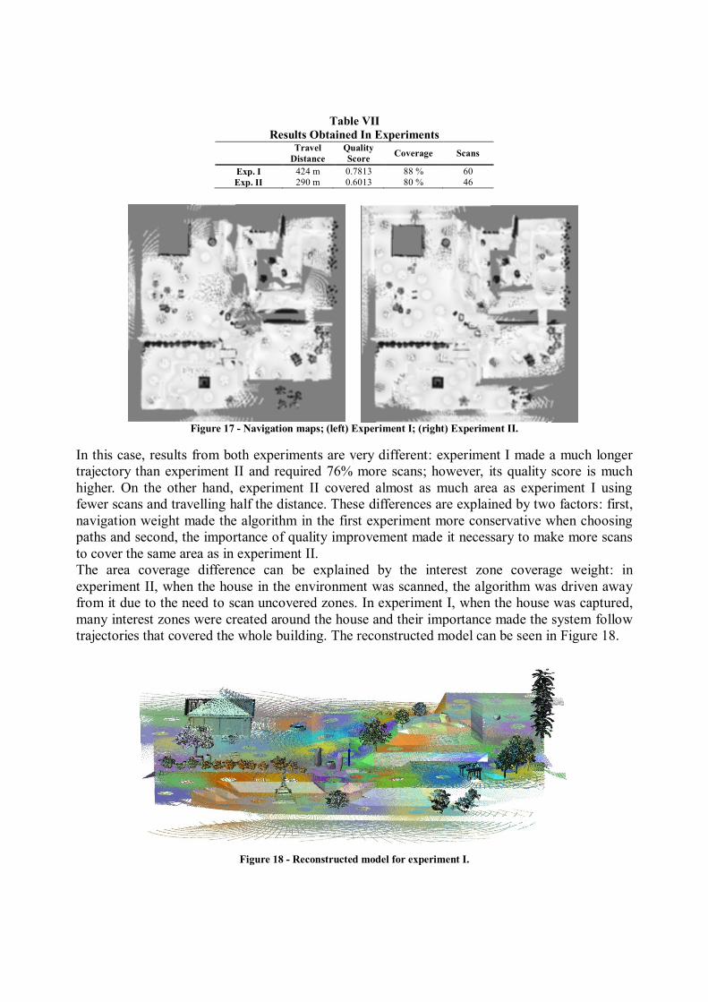
Table VII
Results Obtained In Experiments Travel
Distance
Quality
Score Coverage Scans
Exp. I 424 m 0.7813 88 % 60
Exp. II 290 m 0.6013 80 % 46
Figure 17 - Navigation maps; (left) Experiment I; (right) Experiment II.
In this case, results from both experiments are very different: experiment I made a much longer
trajectory than experiment II and required 76% more scans; however, its quality score is much
higher. On the other hand, experiment II covered almost as much area as experiment I using
fewer scans and travelling half the distance. These differences are explained by two factors: first,
navigation weight made the algorithm in the first experiment more conservative when choosing
paths and second, the importance of quality improvement made it necessary to make more scans
to cover the same area as in experiment II.
The area coverage difference can be explained by the interest zone coverage weight: in
experiment II, when the house in the environment was scanned, the algorithm was driven away
from it due to the need to scan uncovered zones. In experiment I, when the house was captured,
many interest zones were created around the house and their importance made the system follow
trajectories that covered the whole building. The reconstructed model can be seen in Figure 18.
Figure 18 - Reconstructed model for experiment I.

4.3 Real Environments
We have carried out experiments in two real environments. The first one is around the building
of the CARTIF Foundation at Boecillo, Spain. This place was selected for several reasons, apart
from being a very accessible place for our tests: it is a geometrically well defined building
complex with access paths and grass all around which is useful to test our floor detection
algorithm, and there are some obstacles and slopes suitable for testing the trajectory cost
estimation system. Finally, even though it is geometrically simple, it still has several occlusion
planes that are interesting to test the algorithm’s performance on occlusions. The scanning site
can be seen in Figure 19.
The second environment is an abandoned building called “El Pinaron” at Viana de Cega, Spain.
This place was selected because it would be an interesting rescue scenario with a big structure
surrounded by many trees and rubble, with different terrain heights and several occlusion planes.
The scanning site can be seen in Figure 25.
4.3.1. CARTIF Foundation Site
Two different experiments have been carried out in this environment. The parameter values for
the experiments were chosen to achieve different objectives. In the first experiment, the
parameters were set to maximize the amount of information captured on each scan while, at the
same time, reduce trajectory costs; in the second experiment, model quality was given more
importance than the other parameters in order to obtain a good model of the site. However, the
importance of trajectory cost was also increased. The selected values can be seen in Table VIII.
Table VIII
Parameters Used In The Experiments
wA wQ wO wC Scans
Exp. I 0.84 0.10 0.05 0.05 15 Exp. II 0.35 0.40 0.15 0.40 55
Figure 19 – CARTIF Foundation site.
Extraction of safe navigation zones and obstacles
The results obtained from this process in this scenario can be seen in Figure 20 and they show
that our method can detect safe navigation zones and obstacles in real terrains with different

heights and slopes. It can also be observed that obstacle detection is valid for objects at different
heights and with different sizes.
Figure 20 - Result of the ground (left) and obstacle (right) detection methods on a real scan. warmer colours represent
detected surfaces
Using these data, a 2D navigation map was created (see Figure 21). The result is a good quality
map, useful for path planning. It is also a proper plant map of the environment. When the
proposed 2D navigation map is compared to typical occupancy grid maps, it is possible to see
how the navigability concept is applied.
(a)
(c)
(b)
Figure 21 - (a) Aerial view of the CARTIF Foundation site. (b) resulting 2D navigation map. (c) Comparative image between the obtained map and the aerial view of the environment.
Exploration Process Results
Figure 22 shows the trajectory that the robot followed and the final model for experiment I. In
the left image, colder colours represent higher quality scores and the magenta line shows the
robot’s trajectory. In the right image, each captured point cloud is represented by a different
colour.

Figure 22 - Trajectory covered by the robot (in purple) in experiment I, where information gain was the most relevant criterion (left). Waypoints where scans were made are numbered in grey. Resulting model for the experiment (Right).
Figure 23 - Left. Resulting model quality score, colder colours represent higher quality. Right. Robot trajectory form
point starting at point S.
Figure 23 shows the trajectory that the robot followed for experiment II. In the left image, colder
colours represent higher quality scores, while in the right image, the magenta line shows the
robot’s trajectory. Figure 24, represents the final model after this test, where each captured point
cloud is represented by a different colour.
Figure 24 - Resulting model for experiment II

In this case, both experiments provided very different results. The first and most relevant factor
for this difference is that, in experiment II, quality was the dominating factor, which, along with
an increment of the weight of the cost estimation factor, results in candidate targets close to the
robot location to obtain a clear advantage over any other targets. However, in experiment I,
quality was not really important compared to the information gain, which gave a clear offset to
the score of the targets at the frontier between the known and unknown space. The second factor
for the said difference is that the penalty that the robot turns had for the trajectory cost estimation
factor, pushed the robot continuously towards the frontier of the known space, leaving unscanned
candidate locations that would be interesting for the first experiment. However, the quality of the
final model was acceptable. These results show that parameter tuning allows the system to
behave in different ways, depending on the final concrete application of the system.
4.3.2. “El Pinaron”
Figure 25 - "El Pinaron" site
This site (see Figure 25) is a very interesting and challenging environment, since it has a big
structure with long sides surrounded by trees and different obstacles, on a terrain with some
slope and several occlusion planes. Moreover, it is an abandoned building, with through-time
deteriorated structures access paths, which represents a perfect scenario for safety or rescue
robotics.
In order to test how our system performs against typical stationary setups, we have designed an
emergency simulacrum on which a collapsing building has to be quickly reconstructed to
evaluate possible risks. For this test, we have used both our robot and a stationary system
controlled by an experienced operator. First, we will show our system’s performance on safe
navigation zones extraction and exploration while reconstructing the environment. Then, we will
comment on the performance of the stationary system, and finally, we will compare both
scenarios by taking into account the comments made by the stationary system operator.
For the robotic exploration, we have set the parameters in a balanced way in order to maximize
the amount of information captured on each scan while reducing trajectory costs. The selected
parameter values can be seen in Table IX.
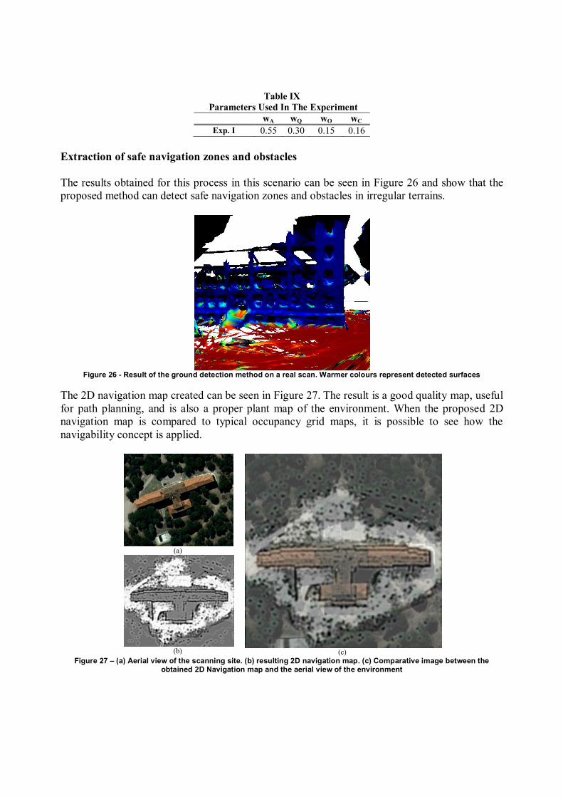
Table IX
Parameters Used In The Experiment
wA wQ wO wC
Exp. I 0.55 0.30 0.15 0.16
Extraction of safe navigation zones and obstacles
The results obtained for this process in this scenario can be seen in Figure 26 and show that the
proposed method can detect safe navigation zones and obstacles in irregular terrains.
Figure 26 - Result of the ground detection method on a real scan. Warmer colours represent detected surfaces
The 2D navigation map created can be seen in Figure 27. The result is a good quality map, useful
for path planning, and is also a proper plant map of the environment. When the proposed 2D
navigation map is compared to typical occupancy grid maps, it is possible to see how the
navigability concept is applied.
(a)
(c)
(b)
Figure 27 – (a) Aerial view of the scanning site. (b) resulting 2D navigation map. (c) Comparative image between the obtained 2D Navigation map and the aerial view of the environment

Exploration Process Results
Figure 28 shows the trajectory that the robot followed and the final model for robotic
exploration. In the image, colder colours represent higher quality scores and the magenta line
shows the robot’s trajectory.
Figure 28 - Resulting Trajectory and model quality score, colder colours represent higher quality
The resulting trajectory shows that the robot can efficiently reconstruct a cluttered environment
moving on rough terrain. The coverage for this environment was 62% of the explorable cells and
the distance travelled was 690 m. Some zones left uncovered were detected as untraversable
because of high soil, and tree density as seen in the navigation map (Figure 27, right). Figure 29
shows the resulting model after the exploration process.
Figure 29 - 3D Model Captured by the Robotic System
Stationary System Reconstruction
For the stationary system, an expert operator using a LEICA HDS-3000 system made a partial
reconstruction of the same environment, the results of which can be seen in Figure 30. The Leica
system has a reach of 100m and can reach resolutions of 1 mm2
from that distance, so the
captured model had a quality that our system cannot reach. On the other hand, it needs a 5
minute setup time and, for this model, each scan required 15 minutes. Once every scan was
captured, the system had to be shut down and manually taken to the new location where the
whole process had to be repeated. The weight of the scanning system (13 kg) and its batteries (8
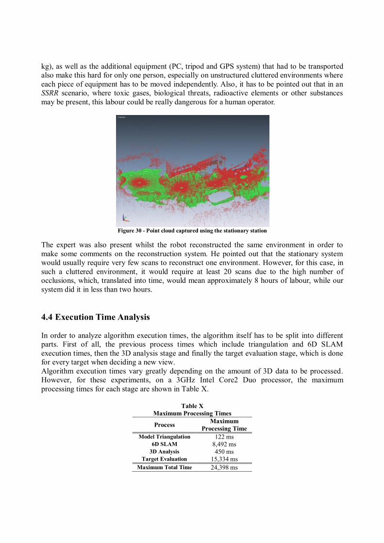
kg), as well as the additional equipment (PC, tripod and GPS system) that had to be transported
also make this hard for only one person, especially on unstructured cluttered environments where
each piece of equipment has to be moved independently. Also, it has to be pointed out that in an
SSRR scenario, where toxic gases, biological threats, radioactive elements or other substances
may be present, this labour could be really dangerous for a human operator.
Figure 30 - Point cloud captured using the stationary station
The expert was also present whilst the robot reconstructed the same environment in order to
make some comments on the reconstruction system. He pointed out that the stationary system
would usually require very few scans to reconstruct one environment. However, for this case, in
such a cluttered environment, it would require at least 20 scans due to the high number of
occlusions, which, translated into time, would mean approximately 8 hours of labour, while our
system did it in less than two hours.
4.4 Execution Time Analysis
In order to analyze algorithm execution times, the algorithm itself has to be split into different
parts. First of all, the previous process times which include triangulation and 6D SLAM
execution times, then the 3D analysis stage and finally the target evaluation stage, which is done
for every target when deciding a new view.
Algorithm execution times vary greatly depending on the amount of 3D data to be processed.
However, for these experiments, on a 3GHz Intel Core2 Duo processor, the maximum
processing times for each stage are shown in Table X.
Table X
Maximum Processing Times
Process Maximum
Processing Time
Model Triangulation 122 ms 6D SLAM 8,492 ms
3D Analysis 450 ms Target Evaluation 15,334 ms
Maximum Total Time 24,398 ms

These results show that the algorithm can be executed online and that it does not delay the
process much, especially considering that these are the worst cases for every process.
5. Conclusion
A method for the automatic reconstruction of outdoor environments has been presented. This
method introduces an algorithm for efficiently planning viewpoints from available 3D data.
Different criteria are used by this algorithm in order to obtain a model with a quality factor over
a minimum desired value. The trajectory that the robot must follow to reach each possible target
is also considered, so that the process keeps an accurate balance between the utility of a point
and the cost of getting to it.
The way 3D data is processed in order to quantify the model quality and extract navigation
surfaces, obstacles and interest regions has been discussed. A navigation map useful for 3D
environments and its resemblance to 2D occupancy grid maps has also been introduced.
The obtained results show that our method can automatically reconstruct an outdoor 3D scene by
calculating efficient trajectories for the robot, and that these trajectories change according to the
chosen parameters to fulfill the desired criteria.
Our future work research will focus on optimizing the evaluation functions in order to make
target evaluation parameters more lineal. We also believe that creating a learning system for
training these parameters to imitate an expert user viewpoint selection could be a challenging
research line.
Semantic labelling of objects from 3D clouds is also interesting and it could, in the future, help
to develop new exploration techniques that consider many new different situations when
evaluating the target. Finally, it may be interesting to work on an extension of this algorithm that
can take into account other sensor readings that may be necessary for evaluating the
environmental situation.
Acknowledgement
The authors would like to thank Mr. Jose Maria Llamas Fernandez for his help on evaluating our
system against stationary laser scanning technology, and for many other useful
recommendations. This work has been partially supported by the Spanish Comisión
Interministerial de Ciencia y Tecnología, (CICYT) under Project DPI2008-06738-C01.
REFERENCES
Basilico, N., & Amigoni, F. (2009). Exploration strategies based on multicriteria decision making
for an autonomous mobile robot. Proceedings of ECMR, 2009, (pp. 259 - 264).
Blaer, P. S., & Allen, P. K. (2007). Data Acquisition and View Planning for 3-D Modeling Tasks.
IROS. San Diego, CA: IEEE/RSJ.
Blaer, P. S., & Allen, P. K. (2009). View Planning and Automated Data Acquisition for Three-
Dimensional Modeling of Complex Sites. Journal of Field Robotics , 26 (11–12), 865–891.

Bourque, E., & Dudek, G. (1998). Viewpoint selection-an autonomous robotic system for virtual
environment creation. IROS (pp. 526–532). IEEE.
Danner, T., & Kavraki, L. E. (2000). Randomized Planning for Short Inspection Paths.
Proceedings of IEEE International Conference on Robotics and Automation ICRA.
Dellaert, F. (2005). 4D cities spatio–temporal reconstruction from images. Recuperado el 10 de
11 de 2010, de http://www.cc.gatech.edu/4d-cities/
Früh, C., & Zakhor, A. (2003). Constructing 3D City Models by Merging Ground-Based and
Airborne Views. IEEE Computer Society Conference on Computer Vision and Pattern
Recognition (CVPR '03), (p. 562).
Gonzalez-Baños, H. H., & Latombe, J. C. (2002). Navigation strategies for exploring indoor
environments. International Journal of Robotics Research , 21, 829–848.
Grabowski, R., Khosla, P., & Choset, H. (2003). Autonomous exploration via regions of interest.
Proceedings of International Conference on Intelligent Robots and Systems (IROS 2003)
(pp. 27–31). IEEE/RSJ.
Hertzberg, J., Lingemann, K., Christopher, L., Nüchter, A., & Stiene, S. (2008). Does It Help a
Robot Navigate to Call Navigability an Affordance? In Towards Affordance-Based Robot
Control (pp. 16-26). Springer Berlin / Heidelberg.
Jensen, B., Weingarten, J., Kolski, S., & Siegwart, R. (2005). Laser range imaging using mobile
robots: From pose estimation to 3D-models. 1st Range Imaging Research Day, (pp. 129-
144). Zurich, Switzerland.
Newman, P., Bosse, M., & Leonard, J. (2003). Autonomous feature-based exploration.
Proceedings of the IEEE International Conference on Robotics and Automation, ICRA03
(pp. 1234–1240). IEEE.
Nüchter, A., Lingemann, K., & Hertzberg, J. (2006). Extracting drivable surfaces in outdoor 6d
slam. 37nd International Symposium on Robotics (ISR ’06). Munich, Germany.
Nüchter, A., Lingemann, K., Hertzberg, J., & Surmann, H. (2007). 6D SLAM - 3D mapping
outdoor environments. Journal of Field Robotics , 24 (8-9), 699 - 722.
Ohno, K., Tadokoro, S., Nagatani, K., Koyanagi, E., & Yoshida, T. (2009). 3-D mapping of an
underground mall using a tracked vehicle with four sub-tracks. 2009 IEEE International
Workshop on Safety, Security & Rescue Robotics (SSRR), (pp. 1-6). Denver, CO.
Pathak, K., Birk, A., Vaskevicius, N., Pfingsthorn, M., Schwertfeger, S., & Poppinga, J. (2010).
Online three-dimensional SLAM by registration of large planar surface segments and
closed-form pose-graph relaxation. Journal of Field Robotics , 27 (1), 52--84.
Pfaff, P., Triebel, R., Stachniss, C., Lamon, P., Burgard, W., & Siegwart, R. (2007). Towards
Mapping of Cities. IEEE International Conference on Robotics and Automation, (pp. 4807-
4813). Roma.
Rusinkiewicz, S. (n.d.). Trimesh2. Retrieved 11 16, 2010, from
http://www.cs.princeton.edu/gfx/proj/trimesh2/
Simmons, R. (2009, 11 9). Inter Process Communication (IPC). Retrieved 11 16, 2010, from
http://www.cs.cmu.edu/~IPC/
Smith, R. (2007, May 28). Open Dynamics Engine (ODE). Retrieved 11 16, 2010, from
http://www.ode.org/
Teller, S. (1997). Automatic acquisition of hierarchical, textured 3D geometric models of urban
environments: Project Plan. Proceedings of the Image Understanding Workshop. New
Orleans.

Tovey, C., & Koenig, S. (2003). Improved Analysis of Greedy Mapping. IEEE/RSJ International
Conference on Intelligent Robots and Systems.
Williams, M. (2010). Street View: Explore the world at street level. Retrieved November 10,
2010, from Google Street View Web page:
http://maps.google.es/intl/en_us/help/maps/streetview/
Yamauchi, B. (1997). A frontier-based approach for autonomous exploration. International
Symposium on Computational Intelligence in Robotics and Automation, ICRA97, (pp. 146–
151).
Yamauchi, B., Schultz, A., Adams, W., & Graves, K. (1998). Integrating map learning,
localization and planning in a mobile robot. Intelligent Control (ISIC), (pp. 331–336).