a nonparametric statistical methodology for the design and analysis of final status
TRANSCRIPT
NUREG-1505, Rev. 1
A Nonparametric StatisticalMethodology for the Designand Analysis of Final StatusDecommissioning Surveys
Interim Draft Report for Comment and Use
U.S. Nuclear Regulatory Commission
Office of Nuclear Regulatory Research
C.V. Gogolak, G.E. Powers, A.M. Huffert

AVAILABILITY NOTICE
Availability of Reference Materials Cited in NRC Publications
Most documents cited in NRC publications will be available from one of the following sources:
1. The NRC Public Document Room, 2120 L Street, NW., Lower Level, Washington, DO20555-0001
2. The Superintendent of Documents, U.S. Government Printing Office, P. 0. Box 37082,Washington, DO 20402-9328
3. The National Technical Information Service, Springfield, VA 22161-0002
Although the listing that follows represents the majority of documents cited in NRC publica-tions, it is not intended to be exhaustive.
Referenced documents available for inspection and copying for a fee from the NRC PublicDocument Room include NRC correspondence and internal NRC memoranda; NRC bulletins,circulars, information notices, inspection and investigation notices; licensee event reports;vendor reports and correspondence; Commission papers; and applicant and licensee docu-ments and correspondence.
The following documents in the NUREG series are available for purchase from the GovernmentPrinting Office: formal NRC staff and contractor reports, NRC-sponsored conference pro-ceedings, international agreement reports, grantee reports, and NRC booklets and bro-chures. Also available are regulatory guides, NRC regulations in the Code of Federal Regula-tions, and Nuclear Regulatory Commission Issuances.
Documents available from the National Technical Information Service include NUREG-seriesreports and technical reports prepared by other Federal agencies and reports prepared by theAtomic Energy Commission, forerunner agency to the Nuclear Regulatory Commission.
Documents available from public and special technical libraries include all open literatureitems, such as books, journal articles, and transactions. Federal Register notices, Federaland State legislation, and congressional reports can usually be obtained from these libraries.
Documents such as theses, dissertations, foreign reports and translations, and non-NRC con-ference proceedings are available for purchase from the organization sponsoring the publica-tion cited.
Single copies of NRC draft reports are available free, to the extent of supply, upon writtenrequest to the Office of Administration, Distribution and Mail Services Section, U.S. NuclearRegulatory Commission, Washington DO 20555-0001.
Copies of industry codes and standards used in a substantive manner in the NRC regulatoryprocess are maintained at the NRC Library, Two White Flint North, 11545 Rockville Pike, Rock-ville, MD 20852-2738, for use by the public. Codes and standards are usually copyrightedand may be purchased from the originating organization or, if they are American NationalStandards, from the American National Standards Institute, 1430 Broadway, New York, NY10018-3308.

NUREG-1505, Rev. 1
A Nonparametric StatisticalMethodology for the Designand Analysis of Final StatusDecommissioning Surveys
Interim Draft Report for Use and Comment
Manuscript Completed: June 1998Date Published: June 1998
Prepared byC.V. Gogolak*, G.E. Powers, A.M.Huffert
Division of Regulatory ApplicationsOffice of Nuclear Regulatory ResearchU.S. Nuclear Regulatory CommissionWashington, DC 20555-0001
*U.S. Department of Energy, Environmental Measurements Laboratory201 Varick Street, 5th FloorNew York, NY 10014

)

ABSTRACT
This report describes a nonparametric statistical methodology for the design and analysis of finalstatus decommissioning surveys in support of the final rulemaking on Radiological Criteria forLicense Termination published by the Nuclear Regulatory Commission in the Federal Registeron July 21, 1997. The techniques described are expected to be applicable to a broad range ofcircumstances, but do not preclude the use of alternative methods as particular situations maywarrant. Nonparametric statistical methods for testing compliance with decommissioning criteriaare provided both for the case in which the radionuclides of concern occur in background andalso for the case in which they do not occur in background. The tests described are the Sign test,the Wilcoxon Rank Sum test, and a Quantile test. These tests are performed in conjunction withan Elevated Measurement Comparison to provide confidence that the radiological criteriaspecified for license termination are met. The Data Quality Objectives process is used for theplanning of final site surveys. This includes methods for determining the number of samplesneeded to obtain statistically valid comparisons with decommissioning criteria and the methodsfor conducting the statistical tests with the resulting sample data.
°°° NUREG-1505

CONTENTS
ABSTRACT ................................. iiiFOREWORD ................................ xiiiABBREVIATIONS...................................................... xiv
I INTRODUCTION..................................................... 1-11.1 Overview of NRC Site Decommissioning ............................. 1-11.2 Need for This Report ............................................ 1-21.3 Objective of This Report.......................................... 1-21.4 Structure of This Report.......................................... 1-3
2 OVERVIEW OF FINAL STATUS SURVEY DESIGN.......................... 2-12.1 Introduction ........................ ....... *2-12.2 Final Status Survey Design........................................ 2-1
2.2.1 Release Criteria.......................................... 2-22.2.2 Data Interpretation ........................................ 2-32.2.3 Survey Unit Classification.................................. 2-32.2.4 Final Status Survey Classification ............................ 2-52.2.5 Background ............................................ 2-62.2.6 Data Variability.......................................... 2-72.2.7 Reference Areas......................................... 2-72.2.8 Radionuclide-Specific Measurements.......................... 2-8
2.3 Statistical Concepts ............................................. 2-82.3.1 Null and Alternative Hypotheses ............................. 2-82.3.2 Decision Errors......................................... 2-10
2.4 Hypothesis Testing Example...................................... 2-li2.4.1 Detection Limits........................................ 2-122.4.2 Final Status Surveys ..................................... 2-142.4.3 The Effect of Measurement Variability on the Decision Process ...... 2-16
2.5 Statistical Tests................................................ 2-172.5.1 Nonparametric Statistical Tests ............................. 2-182.5.2 Wilcoxon Rank Sum and Sign Tests ........................... 2-192.5.3 Mean and Median ....................................... 2-212.3.4 Estimating the Amount of Residual Radioactivity ................ 2-232.5.5 Quantile Test ...................................... 2-232.5.6 Elevated Measurements Comparison .......................... 2-242.5.7 Investigation Levels....................................... 2-25
3 PLANNING FINAL STATUS SURVEYS: DATA QUALITY OBJECTIVES .......... 3-13.1 Introduction..................................................... 3-13.2 State the Problem................................................. 3-23.3 Identify the Decision ..................... ...... 3-23.4 Identify Inputs to the Decision....................................... 3-33.5 Define the Study Boundaries ........................................ 3-5
3.5.1 Spatial Variability ......................................... 3-5
v NUJREG-1 505

CONTENTS
Page3.5.2 Temporal Variability ......................................... 3-63.5.3 Reference Coordinates ....................................... 3-63.5.4 Sampling Grids ...... ...................................... 3-9
3.6 Develop a Decision Rule ............................................ 3-123.7 Specify Limits on Decision Errors .................................... 3-14
3.7.1 Type I and Type H Decision Errors for Statistical Tests ............ 3-143.7.2 Decision Errors for Elevated Areas ............................ 3-19
3.8 Optimize the Design ............................................... 3-213.8.1 Optimizing the Design for the Mean Concentration ............... 3-223.8.2 Optimizing the Design for Detecting Elevated Areas .............. 3-27
4 ANALYSIS OF FINAL STATUS SURVEY RESULTS:DATA QUALITY ASSESSMENT ...................................... 4-1
4.1 Review the Data Quality Objectives (DQOs) and Sampling Design ........... 4-14.2 Conduct a Preliminary Data Review .................................... 4-2
4.2.1 Basic Statistical Quantities .................................... 4-34.2.2 Graphical Data Review ....................................... 4-7
4.3 Select the Statistical Test ............................................ 4-134.4 Verify the Assumptions of the Statistical Test ........................... 4-154.5 Draw Conclusions from the Data ...................................... 4-16
5 SIGN TEST: CONTAMINANT NOT PRESENT IN BACKGROUND ............... 5-15.1 Introduction ....................................................... 5-15.2 Applying the Sign Test: Scenario A .................................... 5-55.3 Applying the Sign Test: Scenario B ..................................... 5-75.4 Interpretation of Test Results ........................................... 5-8
5.4.1 If the Null Hypothesis Is Not Rejected ........................... 5-95.4.2 If the Null Hypothesis Is Rejected ............................. 5-10
6 WILCOXON RANK SUM TEST: CONTAMINANT PRESENT IN BACKGROUND ... 6-16.1 Introduction ....................................................... 6-16.2 Applying the WRS Test: Scenario A ................................... 6-56.3 Applying the WRS Test: Scenario B ................................... 6-96.4 Interpretation of Test Results .......................................... 6-13
6.4.1 If the Null Hypothesis Is Not Rejected .......................... 6-136.4.2 If the Null Hypothesis Is Rejected ............................. 6-13
7 QUANTILE TEST ......................................................... 7-17.1 Introduction ....................................................... 7-17.2 Applying the Quantile Test ........................................... 7-17.3 Calculation of aQ for the Quantile Test .................................. 7-37.4 Modified Example for the Quantile Test ................................ 7-5
8 ELEVATED MEASUREMENT COMPARISON ................................. 8-18.1 Introduction ........................................................ 8-18.2 Comparison against Individual Measurements ............................ 8-2
NUREG-1505 vi

CONTENTS
Page8.3 Comparison Against Scanning Measurements............................. 8-48.4 Area Factors ................................................... 8-48.5 Example ................................................ 8-9
9 SAM PLE SIZE ................................... .......................... 9-19.1 Sample Size and Decision Errors ...................................... 9-19.2 Sample Size Calculation for the Sign Test Under Scenario A ................ 9-29.3 Sample Size Calculation for the Sign Test Under Scenario B .............. 9-79.4 Sample Size Calculation for the WRS Test Under Scenario A ............... 9-99.5 Sample Size Calculation for the WRS Test Under Scenario B .............. 9-14
10 POWER CALCULATIONS FOR THE STATISTICAL TESTS ................... 10-110.1 Statistical Power and the Probability of Survey Unit Release ............. 10-110.2 Power of the Sign Test Under Scenario A ............................. 10-110.3 Power of the Sign Test Under Scenario B ............................. 10-410.4 Power of the Wilcoxon Rank Sum Test Under Scenario A ................ 10-610.5 Power of the Wilcoxon Rank Sum Test Under Scenario B .............. 10-12
11 MULTIPLE RADIONUCLIDES ........................................... 11-111.1 Using the Unity Rule .............................................. 11-111.2 Radionuclide Concentrations With Fixed Ratios ........................ 11-111.3 Unrelated Radionuclide Concentrations ............................... 11-211.4 Example Application of WRS Test to Multiple Radionuclides .............. 11-3
12 M'ULTIPLE SURFACES .......................................... 12-1\12.1 Choosing Survey Units .......... ........................... 12-112.2 Combining Dissimilar Areas into One Survey Unit ................. ..... 12-112.3 Using Paired Observations for Survey Units with Many Different Backgrounds 12-4
13 DEMONSTRATING INDISTINGUISHABILITY FROM BACKGROUND ......... 13-113.1 Determining Significant Background Variability ........................ 13-113.2 Determining if Reference Areas Have Significantly Different Background .... 13-213.3 Establishing the Concentration Level that Is Indistinguishable ............. 13-513.4 Using the Concentration Level that Is Indistinguishable in the WRS Test .... 13-913.5 Determining the Number of Reference Areas and the Number of Samples . 13-1113.6 Determining when Demonstrating Indistinguishability Is Appropriate ........ 13-12
14 ALTERNATIVES AND MODIFICATIONS ............................. 14-114.1 Alternative Statistical Tests ................................... 14-114.2 Retesting ....................................................... 14-314.3 Composite Sampling ......... .............................. 14-3
15 GLOSSARY ............................................................. 15-1
16 BIBLIOGRAPHY ........................................................ 16-1
APPENDIX: STATISTICAL TABLES ......................................... A-1
vii NUREG-1505

CONTENTS
FIGURESPage
Figure 2.1 Type I and Type II Errors in the Determination of a Detection Limit ......... 2-13Figure 2.2 Type I and Type II Errors for Scenario A ................................ 2-14Figure 2.3 Type I and Type II Errors for Scenario B ............................... 2-15Figure 2.4 Differences in Concentration Compared to Measurement Variability .......... 2-17Figure 2.5 Comparison of Normal and Lognormal Distributions ...................... 2-22
Figure 3.1 Sample Indoor Reference Coordinate System ............................. 3-7Figure 3.2 Sample Outdoor Reference Coordinate System.......................... 3-8Figure 3.3 Laying Out a Triangular Grid ..................................... 3-11Figure 3.4 Completed Triangular Sampling Pattern ................................ 3-12Figure 3.5 Example of Setting Acceptable Probabilities for Survey Unit Release ......... 3-16Figure 3.6 Circular and Elliptical Areas Relative to the Sample Grid ................. 3-19Figure 3.7 Probability that an Elliptical Area Is Not Sampled on a Triangular Grid 3-20Figure 3.8 Probability that a Circular Area Is Not Sampled on a Systematic Grid ......... 3-21Figure 3.9 Probability that a Survey Unit Is Released Using Sign Test Under Scenario A .. 3-26Figure 3.10 Probability that a Survey Unit Is Released Using Sign Test Under Scenario B . 3-27Figure 3.11 Probability that a Survey Unit Is Released Using WRS Test Under Scenario A 3-28Figure 3.12 Probability that a Survey Unit Is Released Using WRS Test Under Scenario B . 3-29
Figure 4.1 Confidence Bands for the Ratio of the Range to the Standard Deviation ........ 4-7Figure 4.2 Example of a Posting Plot ....................................... 4-9Figure 4.3 Frequency Plots of Example Survey Unit Data ........................ 4-10Figure 4.4 Ranked Data Plot for the Example Reference Area Data ................... 4-12Figure 4.5 Ranked Data Plot for the Example Survey Unit Data ...................... 4-12Figure 4.6 Example Quantile-Quantile Plot ................................... 4-14
Figure 5.1 Desired Probability That the Survey Unit Passes ........................... 5-2Figure 5.2 Posting Plot of Survey Unit Data ....................................... 5-2Figure 5.3 Histogram of Survey Unit Data ........................................ 5-4Figure 5.4 Ranked Data Plot of Survey Unit Data .................................. 5-5
Figure 6.1 Desired Probability That the Survey Unit Passes ......................... 6-2Figure 6.2 Posting Plot of Reference Area and Survey Unit Data ...................... 6-3Figure 6.3 Histograms of Reference Area and Survey Unit Data ....................... 6-4Figure 6.4 Quantile-Quantile Plot of Example Data ................................. 6-5
Figure 8.1 Square and Triangular Sampling Grids and Grid Areas ....................... 8-3Figure 8.2 Example Outdoor Area Factors ........................................ 8-7Figure 8.3 Example Indoor Area Factors ........................................... 8-8Figure 8.4 Combined Ranked Data Plot of Reference Area and Survey Unit Measurements- .8-10Figure 8.5 Posting Plot of Indoor Concrete Survey Unit ............................. 8-12
Figure 9.1 The Parameter p for the Sign Test Under Scenario A ....................... 9-4Figure 9.2 Sample Size Multiplier and the Parameter p Versus A/c .................... 9-5Figure 9.3 Dependence of Sample Size on p ................................... 9-6
NUREG-1505 viii

CONTENTS
FIGURES (cont'd.)Page
Figure 9.4 The Parameter p for the Sign Test Under Scenario B ...................... 9-8Figure 9.5 The Parameter P,. for the WRS Test Under Scenario A.....................9-10Figure 9.6 Dependence of Sample Size on A/o for WRS Test ........................ 9-12Figure 9.7 Comparison of Sample Sizes Required for the WRS Test and the Sign Test .... 9-13Figure 9.8 Dependence of Sample Size on Pr ............ .......................... 9-14Figure 9.9 The Parameter Pr for the WRS Test Under Scenario B .................... 9-15
Figure 10.1 Example Power Curves: Sign Test Scenario A .......................... 10-3Figure 10.2 Example Power Curves: Sign Test Scenario B .......................... 10-7Figure 10.3 Probability Example Survey Unit Passes: Sign Test Scenario B ............ 10-7Figure 10.4 Example Power Curves: WRS Test Scenario A ........................ 10-12Figure 10.5 Example Power Curves: WRS Test Scenario B ........................ 10-15Figure 10.6 Probability Example Survey Unit Passes: WRS Test Scenario B ........... 10-16
Figdre 12.1 Example Survey Units: Case #1 ...................................... 12-2Figure 12.2 Example Survey Units: Case #2 ...................................... 12-3Figure 12.3 Example Survey Units: Case #3 ...................................... 12-3Figure 12.4 Example Survey Units: Case #4 ...................................... 12-5
Figure 13.1 Impact of Background on Decision Errors .............................. 13-2Figure 13.2 Example DQOs for the Probability That the Survey Unit Passes Versus the
Concentration Difference Between the Survey Unit and the Reference Area .. 13-10
TABLES
Table 2.1 Final Status Survey Design Classification ................................. 2-5Table 2.2 Summary of Types of Decision Errors .................................. 2-11Table 2.3 Summary of Statistical Tests .......................................... 2-18Table 2.4 Summary of Investigation Levels ...................................... 2-25
Table 3.1 Summary of Types of Decision Errors . ................................. 3-15Table 3.2 Number of Samples Required for the Sign Test............................ 3-22Table 3.3 Number of Samples Required for the Wilcoxon Rank Sum Test ............... 3-23
Table 4.1 Example Final Status Survey Data ...................................... 4-4Table 4.2 Basic Statistical Quantities Calculated for the Data in Table 4.1 ............... 4-5Table 4.3 Ranks of the Example Data ........................................... 4-11Table 4.4 Recommended Statistical Tests ........................................ 4-15
* Table 4.5 Methods for Checking the Assumptions of Statistical Tests.................. 4-16
Table 5.1 Summary Statistics for Example Data of Figure 5.2 ......................... 5-3Table 5.2 Ranked Data for Example Figure 5.2 ............ ....................... 5-4Table 5.3 Calculations for Sign Test in Scenario A ................................. 5-7Table 5.4 Calculations for Sign Test in Scenario B .............. .................... 5-9
ix NUREG-1505

CONTENTS
TABLES (cont'd.)
Table 6.1 Summary Statistics for Example Data of Figure 6.2 ..................... 6-3Table 6.2 Ranked Data for Example of Figure 6.2 .................................. 6-4Table 6.3 WRS Test for Class 2 Interior Drywall Survey Unit ........................ 6-7Table 6.4 Spreadsheet Formulas Used in Table 6.3 ................................. 6-8Table 6.5 WRS Test Under Scenario B for Class 2 Interior Drywall Survey Unit ........ 6-11Table 6.6 Spreadsheet Formulas Used in Table 6.5 ................................ 6-12
Table 7.1 Quantile Test Under Scenario B for Class 2 Interior Drywall Survey Unit ....... 7-2Table 7.2 Example Calculation of aQ for the Quantile Test ........................... 7-4Table 7.3 Spreadsheet Formulas Used in Table 7.2 ................................. 7-5Table 7.4 Quantile Test Under Scenario B: Modified Example Survey Unit .............. 7-6
Table 8.1 Example Outdoor Area Factors ........................................ 8-6Table 8.2 Example Indoor Area Factors .......................................... 8-8Table 8.3 Data for Indoor Survey Unit and Reference Area ........................... 8-11
Table 9.1 Some Values of Z,, and Z1 _.p Used To Calculate the Sample Sizes ............ 9-2Table 9.2 Some Values of (Z,.,, + Z1 _p) 2 Used To Calculate Sample Sizes ............... 9-3Table 9.3 Values of p for Use in Computing Sample Size for the Sign Test ..... %........ 9-5Table 9.4 Values of P, for Use in Computing Sample Size for the WRS Test ........... 9-11
Table 10.1 Example Power Calculations: Sign Test Scenario A ....................... 10-3Table 10.2 Example Power Calculations: Sign Test Scenario B ...................... 10-6Table 10.3 Values ofp, and P2 for Computing the Mean and Variance of WMW .......... 10-10Table 10.4 Example Prospective Power Calculation: WRS Test Scenario A ............ 10-11Table 10.5 Example Prospective Power Calculation: WRS Test Scenario B ............ 10-15
Table 11.1 Example WRS Test for Two Radionuclides ............................. 11-4
Table 13.1 Critical Values, K,, for the Kruskal-Wallis Test ......................... 13-4Table 13.2 Example Data for the Kruskal-Wallis Test .............................. 13-5Table 13.3 Calculation of 02 for the Example Data ............................ 13-8Table 13.4 Analysis of Variance for Example Data ................................ 13-9Table 13.5 Power of the F-test When c2 = o2 .................................... 13-12
Table A.1 Cumulative Normal Distribution Function, 4)(z) ........................... A-1Table A.2a Sample Sizes for the Sign Test ....................................... A-2Table A.2b Sample Sizes for the Wilcoxon Rank Sum Test .......................... A-3Table A.3 Critical Values for the Sign Test Statistic, S - ............................ A-4Table A.4 Critical Values for the WRS Test .... ............................ A-6Table A.5a 0.025 and 0.975 Percentiles of the Chi-Squared Distribution ............... A-9Table A.5b 0.05 and 0.95 Percentiles of the Chi-Squared Distribution ................ A-10Table A.6 1000 Random Numbers Uniformly Distributed Between Zero and One ........ A-11Table A.7a Values of r and k for the Quantile Test When a Is Approximately 0.01 ...... A-13Table A.7b Values of r and k for the Quantile Test When a Is Approximately 0.025 ..... A-14
NUREG-1505 X
CONTENTS
TABLES (cont'd.)Page
Table A.7c Values of r and k for the Quantile Test When a Is Approximately 0.05 ...... A-15Table A.7d Values of r and k for the Quantile Test When a Is Approximately 0. 10 ...... A-16
xi NUREG-1505


FOREWORD
The NRC has amended its regulations to establish residual radioactivity criteria for decommis-sioning of licensed nuclear facilities. As part of this initiative, the NRC staff has evaluated theapplication of nonparametric statistical methods as an alternative to the parametric statisticalapproach described in the U.S. Nuclear Regulatory Commission (NRC) draft reportNUREG/CR-5849, entitled, "Manual for Conducting Radiological Surveys in Support of LicenseTermination." The nonparametric statistical approach described in this report is expected to besimpler and more cost-effective for the design and analysis of final status decommissioningsurveys when radiological criteria for decommissioning approach background radiation levels.This report also shows the advantages of using the Data Quality Objectives process as it relatesto the planning and analysis of final site surveys. The application of the proposed DQO processincludes methods for determining the number of samples needed to obtain statistically validcomparisons with decommissioning criteria and the methods for conducting the statistical testswith the resulting sample data.
The initial draft of this report was published in August 1995. As a result of the commentsreceived, extensive revisions were made to include alternative scenarios for statistical hypothesistesting. A number of new concepts have been introduced, and examples for some special caseshave been added. The results, approaches and methods described herein are provided forinformation only and should not be considered a substitute for NRC requirements.
n W. Craig, DirectorDivision of Regulatory ApplicationsOffice of Nuclear Regulatory Research
Xlll NUREG-1505

ABBREVIATIONS
ALARACFRDCGLDOEDQADQOEMCEPALBGRMCAMDCNISTNRCPCPDLPICQAQCTEDEWRSWSR
as low as is reasonably achievableCode of Federal RegulationsDerived Concentration Guideline LevelU.S. Department of Energydata quality assessmentdata quality objectiveelevated measurement comparisonU.S. Environmental Protection AgencyLower Boundary of the Gray Regionmultichannel analyzerminimum detectable concentrationNational Institute for Standards and TechnologyU.S. Nuclear Regulatory Commissionpersonal computerpredicted dose levelpressurized ionization chamberquality assurancequality controltotal effective dose equivalentWilcoxon Rank Sum TestWilcoxon Signed Ranks Test
NUREG-1505 xiv
1 INTRODUCTION
1.1 Overview of NRC Site Decommissioning
At sites and facilities licensed by the Nuclear Regulatory Commission (NRC), the formaldecommissioning process begins when a licensee decides to terminate licensed activities. Themajority of licenses terminated each year by NRC involve little or no site remediation and,therefore, present no complex decommissioning problems owing to residual radioactivity.However, license termination at a small number of sites is far more complex becausecontamination may be spread into various areas within the facility and surrounding areas by themovement of materials and equipment, by activation, and by the dispersion of air, water, or otherfluids through or along piping, equipment, walls, floors, and drains. Decontamination of suchareas is likely to be performed at nuclear power plants, non-power (research and test) reactors,fuel fabrication plants, uranium hexafluoride production plants, and independent spent fuelstorage installations. A small number of universities, medical institutions, radioactive sourcpmanufacturers, and companies that use radioisotopes for industrial purposes may also containradioactive contamination that requires remediation.
NRC regulations in 10 CFR 30.36, 40.42, 50.82, 70.38, and 72.54 require licensees to removetheir facilities from service safely. As part of the decommissioning process, licensees arerequired to demonstrate that residual radioactivity in facilities and environmental media has beenreduced to acceptable levels. Typically, licensees demonstrate compliance with radiologicalcriteria for license termination by conducting final status surveys of the site or facility andreporting the survey results to NRC for evaluation. Where appropriate, the NRC staff conductsconfirmatory surveys to verify that lands and structures have been adequately remediated.
On July 21, 1997, the NRC amended the regulations in 10 CFR Part 20 to include explicitradiological criteria for decommissioning (62 FR 139, pp. 39057- 39092). Subpart E of theamended regulations contains dose-based radiological criteria for restricted and unrestrictedrelease, consisting of a total effective dose equivalent (TEDE) limit for residual radioactivityabove background. These regulations replace prior NRC guidance based on surface and volumeactivity concentration limits for specific radionuclides.
To implement the dose criteria in the amended 10 CFR Part 20, final status surveys andconfirmatory surveys must be capable of detecting very low levels of residual radioactivity in thepresence of background at a variety of NRC-licensed facilities and sites. An essential componentof such surveys is a statistical methodology that is appropriate for radiological data at or nearbackground levels. This document presents such a methodology.
1.2 Need for This Report
Previously, the NRC staff used guidance for conducting final status radiological surveys that iscontained in draft report NUREG/CR-5849 (1992), entitled "Manual for ConductingRadiological Surveys in Support of License Termination." This report contains an alternativestatistical approach for designing radiological surveys. The framework for the survey design is
1-1 NUREG-1505

INTRODUCTION
the Data Quality Objectives (DQO) process. The DQO process uses statistical hypothesis testingrather than the construction of confidence intervals. This allows a balance to be reached betweenthe risk of possibly releasing an incompletely remediated site and the risk of possibly requiringfurther remediation at an already adequately remediated site. One of the primary goals of theDQO process is the determination of acceptable decision error rates for the hypothesis test, i.e.,those that will reflect the relative importance of these risks at a specific site. The DQO process isused to incorporate site-specific information and sound scientific judgment into the survey designand data analysis so that the objective of safely releasing a site can be met while reducing thenumber of unnecessarily arbitrary and conservative assumptions that are sometimes invoked inthe face of uncertainty.
Using the DQO framework, the amount and type of data to be collected are related to thespecific decision to be made rather than sampling at a fixed density. The number of samples ofmeasurements needed in a survey unit is determined by the acceptable decision error rates, themagnitude of the release criterion relative to the overall variability of the data, and the sensitivityof the scanning method used. The type and amount of scanning required depend primarily on theclassification of the survey unit. Three classes of survey units are used to direct the survey effortat a level commensurate with the potential for residual radioactivity in excess of the releasecriterion. Acceptable areas of elevated activity are determined by radionuclide-specific areafactors derived from an appropriate dose model..
The nonparametric statistical techniques described in this report do not require the data to benormally or log-normally distributed and are, therefore, expected to be more appropriate fordetermining the number of samples required for radiological surveys and analyzing data collectedat or near background levels. These tests perform almost as well as the parametric tests evenwhen the data are normally distributed, are less sensitive to outliers, and are better able to handledata sets that include non-detects.
There are two possible approaches to demonstrating compliance with criteria that specify a doselimit due to residual radioactivity distinguishable from background, depending on which of thefollowing questions is emphasized:
(1) Does the dose due to residual radioactivity exceed the limit?(2) Is the residual radioactivity indistinguishable from background?
In the initial draft of NUREG-1505 (August 1995) the approach emphasized question 2. Thisfinal report addresses both approaches.
1.3 Objective of This Report
This report describes a nonparametric statistical methodology that NRC licensees may considerwhen evaluating methods for demonstrating compliance with the radiological criteria for licensetermination in Subpart E of 10 CFR Part 20. The DQO process (EPA QA/G-4 and QA/G-9,1994) is used as the framework for the planning of final site surveys. The statistical approachdescribed in this report is expected to be a resource-efficient solution for the design of final statusdecommissioning surveys when radiological criteria for decommissioning approach background
NUREG-1505 1-2

INTRODUMTON
levels. The proposed process includes methods for determining the number of samples needed toobtain statistically valid comparisons with decommissioning criteria and the methods forconducting the statistical tests with the resulting sample data.
No single statistical formulation can adequately anticipate every contingency that will arise indeciding whether a survey unit can be safely released. The DQO process should be used todetermine whether a proposed action will further the objective of safely releasing the site. Thedecisions reached may not always be accompanied by a numerical procedure leading to thatdecision. However, such decisions should always be accompanied by a description of whichactions were taken, and why. The DQO process provides a methodology for resolving the oftencomplex issues surrounding site remediation and decommissioning.
1.4 Structure of This Report
This report is divided into four major parts. The first part deals with general final status surveydesign criteria, definitions, and data quality objectives (Chapters 2 and 3). The second partdescribes preliminary data analysis and data quality assessment (Chapter 4). The third partdescribes the use of the statistical tests recommended in this report (Chapters 5 through 8).These first eight chapters contain all of the information required to design and conduct finalstatus surveys, and to analyze and interpret the results. Chapters 9 through 14 deal withextensions of, and alternatives to, the statistical procedures that may be applicable in somesituations. Chapters 15 and 16 contain a Glossary and Bibliography, respectively. The appendixcontains the statistical tables needed to perform the analyses described in this report.
1-3 NUREG- 1505


2 OVERVIEW OF FINAL STATUS SURVEY DESIGN
2.1 Introduction
It is recognized that demonstrating that residual concentrations of radioactivity at a site are atvery low levels in the presence of background may be a complex task involving sophisticatedsampling, measurement, and statistical analysis techniques. The difficulty of the task can varysubstantially depending on a number of factors, including the radionuclides in question, thebackground level for those and other radionuclides at the site, and the temporal and spatialvariations in background at or near the site. Sufficient radiological data must be collected tocharacterize both the residual radioactivity at the site and the background radioactivity levels inthe vicinity of the site. The number of measurements required to accomplish this task will bedetermined on a site-specific basis and will depend upon the nature of the facility, its size, theselection of thestatistical tests used, and certain statistical parameter values that influence howcompliance with radiological criteria is determined.
2.2 Final Status Survey Design
Decommissioning is defined in 10 CFR 20.1003 as removing a facility or site safely from service,and reducing residual radioactivity to a level that permits (1) release of the property forunrestricted use and termination of the license; or (2) release of the property under restrictedconditions and termination of the license. A survey unit is a geographical area of specified sizeand shape for which a separate decision will be made whether or not that area meets the releasecriteria. This decision is made following afinal status survey of the survey unit. Thus, a surveyunit is an area for which a final status survey is designed, conducted, and results in a releasedecision. The objective of this report is the design of efficient final status surveys. These surveysshould obtain all of the data required for making the decision, but avoid the collection andanalysis of superfluous samples.
Usually there are two conditions that would lead to the determination that a particular survey unitrequires further remediation before unrestricted release:
(1) If the average level of residual radioactivity within the survey unit exceeds the regulatorylimit, or
(2) If there are small areas within the survey unit with elevated residual radioactivity thatexceed the regulatory limit.
Sampling at discrete points within the survey unit is a simple method for determining if the firstof these conditions exists. The term sampling is used here in its statistical sense, namelyobtaining data from a subset of a population. Sampling in this sense Would include both direct insitu measurements and the collection of physical samples for laboratory analysis.
On the other hand, sampling at discrete points within a survey unit is not a very efficient methodof determining if the second condition exists. Scanning is a much better method for detectingisolated areas with elevated activity. However, scanning is generally not as sensitive as sampling.
2-1 2-1 NUREG- 1505

OVERVIEW
A major component of the survey designs discussed in this report is the efficient use of samplingat distinct locations combined with scanning to accurately determine the final status of a surveyunit. The statistical procedures described in this report are used to establish the number of ;samples taken at distinct locations needed to determine if the mean concentration in the surveyunit exceeds the regulatory limit, with a specified degree of precision. Thus, these statisticalprocedures are as important in the planning and design of the final status survey as they are in theanalysis and interpretation of the resulting data.
2.2.1 Release Criteria
In the past, release criteria have often been expressed as activity concentration limits. The criteriafor license termination given in 10 CFR 20.1402 and 10 CFR 20.1403 are expressed in terms oftotal effective dose equivalent (TEDE). This cannot be measured directly. Exposure pathwaymodeling is used to calculate the estimated volume or surface area concentration of specificradionuclides that could result in a TEDE equal to the release criterion. This concentration istermed the derived concentration guideline level (DCGL). The units for the DCGL are the sameas the units for measurements performed to demonstrate compliance (e.g., Bq/kg, Bq/m', etc.).This allows direct comparisons between the survey results and the DCGL.
A complete discussion of DCGLs is beyond the scope of this report. There is, however, oneaspect of exposure pathway modeling that bears directly on survey unit design. That is thedependence of the TEDE on the assumed area of contamination used in the exposure pathwaymodel.
The two conditions of Section 2.2 that may cause a survey unit to fail the TEDE release criterionmay have very different corresponding DCGLs because of the different size of the areas ofresidual radioactivity. Consequently, this report considers two distinct DCGLs:
(1) The DCGLw is derived assuming that residual radioactivity is uniformly distributed overa wide area, i.e. the entire survey unit. This can often be the default DCGL provided by anexposure pathway model.
(2) The DCGLEMc is derived assuming that residual radioactivity is concentrated in a muchsmaller area, i.e., in only a small percentage of the entire survey unit.
The DCGLEMc can never be less than the DCGLw, but it may be significantly greater. The ratio ofthe DCGLEMc to the DCGLw defines a radionuclide specific area factor, FA, such that theDCGI-mMc = (FA) (DCGLw), when the residual radioactivity is confined to an area of size A.
Detailed procedures for developing these area factors are beyond the scope of this report.However, in the simplest case, an area factor can be determined from the ratio of the resultobtained from an exposure pathway model using the entire survey unit area to the result obtainedassuming the residual radioactivity is confined to a smaller area. The value of the DCGL EMC thatis calculated for survey planning purposes is based on an area, A, determined by the spacingbetween adjacent sampling locations.
NUREG-1505 2-2

OVERVIEW
2.2.2 Data Interpretation
The use of the two DCGLs discussed above differs when interpreting the results of the finalstatus survey data. The DCGLw is used to form a statistical hypothesis concerning the level ofresidual radioactivity that may be uniformly distributed across the survey unit. A nonparametrictest is applied to the sampling data taken at distinct locations in the survey unit to determinewhether this level meets the release criterion.
The DCGLtmc, however, is used to trigger further investigation of a portion of the survey unit.Any measurement from the survey unit is considered elevated if it exceeds the DCGLmc. This isthe elevated measurement comparison. The existence of an elevated measurement in a surveyunit indicates the possibility of an area of residual radioactivity that may cause the dose criteria tobe exceeded. The elevated measurement alone does not indicate that the survey unit fails to meetthe release criterion, only that it is a possibility that must be investigated further. The DCGLEMCis based on the area factor used for the survey design. The area factor used in the survey design isbased on the area bounded by adjacent sampling points. The actual area of elevated activity couldbe smaller. Thus, the area factor based on the actual area of contamination may be larger.Further investigation will usually be necessary to determine the actual extent and concentrationlevel of a specific elevated area.
2.2.3 Survey Unit Classification
To maximize the efficiency of the final status surveys, it is clear that the greatest effort should beexpended on the areas that have the highest potential for contamination. Final status surveydesigns depend fundamentally on the classification of survey units according to contaminationpotential. The survey unit classification determines the final status survey design and theprocedures used to develop the design.
Areas that have no potential for residual contamination are classified as non-impacted areas.These areas have no radiological impact from site operations and are typically identified early indecommissioning. Areas with some potential for residual contamination are classified asimpacted areas.
Impacted areas are further divided into one of three classifications:
(1) Class 1 Areas: Areas containing locations where, prior to remediation, the concentrationsof residual radioactivity may have exceeded the DCGLW,
(2) Class 2 Areas: Areas containing no locations where, prior to remediation, theconcentrations of residual radioactivity may have exceeded the DCGL W
(3) Class 3 Areas: Areas with a low probability of containing any locations with residualradioactivity.
Class 1 areas have the greatest potential for contamination and therefore receive the highestdegree of survey effort for the final status survey. Non-impacted areas do not receive any level ofsurvey coverage because they have no potential for residual contamination. Impacted areas for
2-3 NUREG-1505

OVERVIEW
which there is insufficient information to justify a lower classification should be classified asClass 1.
Examples of Class 1 areas include: (1) site areas previously subjected to remedial actions,(2) locations where leaks or spills are known to have occurred, (3) former burial or disposal sites,(4) waste storage sites, and (5) areas with contaminants in discrete solid pieces of material andhigh specific activity.
Remediated areas are identified as Class I areas because the remediation process often results inless than 100% removal of the contamination. The contamination that remains on the site afterremediation is often associated with relatively small areas with elevated levels of residualradioactivity. This results in a non-uniform distribution of the radionuclide and a Class 1 -classification. If an area is expected to have levels of residual radioactivity below the DCGL wand was remediated for purposes of ALARA, the remediated area might be classified as Class 2for the final status survey.
Examples of areas that might be classified as Class 2 for the final status survey include:(1) locations where radioactive materials were present in an unsealed form, (2) potentiallycontaminated transport routes, (3) areas downwind from stack release points, (4) upper walls andceilings of buildings or rooms subjected to airborne radioactivity, (5) areas handling lowconcentrations of radioactive materials, and (6) areas on the perimeter of former contaminationcontrol areas.
To justify changing the classification from Class 1 to Class 2, there should be measurement datathat provides a high'degree of confidence that no individual measurement would exceed theDCGLw. Other justifications for reclassifying an area as Class 2 may be appropriate, based onsite-specific considerations.
Examples of areas that might be classified as Class 3 include buffer zones around Class 1 orClass 2 areas, and areas with very low potential for residual contamination but insufficientinformation to justify a non-impacted classification.
The number of distinct sampling locations needed to determine if a uniform level of residualradioactivity within a survey unit exists does not depend on the survey unit size. However, thesampling density within a survey unit should reflect the potential for small elevated areas ofresidual radioactivity. Thus, the appropriate size for survey units formed within each of the threearea classifications differs. Survey units with a higher potential for residual radioactivity shouldbe smaller. Suggested maximum areas for survey units are:
Class 1 Structures ........ 100 m2 floor areaClass 1 Land areas ....... 2,000 m2
Class 2 Structures ........ 100 to 1,000 m2
Class 2 Land areas ....... 2,000 to 10,000 in2
Class 3 Structures ........ no limitClass 3 Land areas ....... no limit
NUREG-1505 2-4

OVERVIEW
The area of the survey unit should also be consistent with that assumed in the exposure pathwaymodel used to calculate the DCGLw. Survey units with structure surface areas less than 10 m 2orland areas less than 100 m2 may have unnecessarily high sampling densities, and should beavoided.
2.2.4 Final Status Survey Classification
Class I areas have the highest potential for containing small areas of elevated activity exceedingthe release criterion. Consequently, both the number of sampling locations and the extent ofscanning effort is the greatest. The final status survey is driven by the effort to providereasonable assurance that if any areas with concentrations in excess of the DCGL EMCexist thatthen these areas will be found. Sampling is done on a systematic grid. The distance betweensampling locations is made small enough that any elevated area that might be missed bysampling would be found by scanning. Scanning is performed over 100% of the survey unit. Theminimum detectable concentration (MDC) of the scanning method must be lower than theDCGLEMC.
Class 2 areas may contain residual radioactivity, but the potential for elevated areas is very small.Sampling is done on a systematic grid. The distance between samples is limited by limiting themaximum size of the survey unit. Scanning is performed systematically over the survey unit.Since Class 2 is an intermediate classification, scanning coverage may range from as little as10% to nearly 100% of the survey unit, depending on whether the potential for an elevated area isnearer that for a Class 1 area or for a Class 3 area.
Class 3 areas should contain little, if any, residual radioactivity. There should be virtually nopotential for elevated areas. Sampling is random across the survey unit, and the sample densitycan be very low. Scanning is limited to those parts of the survey unit where it is deemed prudent,based on the judgment of an experienced professional.
Table 2.1 summarizes the differences in the final status survey design for each of the three survey
unit classifications.
Table 2.1 Final Status Survey Design Classification
Class Sampling Scanning
1 Systematic 100% Coverage
2 Systematic 10- 100%
3 Random Judgmental
2-5 NUREG-1505

OVERVIEW
2.2.5 Background
The release criteria in 10 CFR Part 20.1402 and 1403 specify a dose limit (TEDE) due to residualradioactivity that is distinguishable from background radiation. According to 10 CFR 20.1003,background radiation means radiation from cosmic sources, naturally occurring radioactivematerial, including radon (except as a decay product of source or special nuclear material), andglobal fallout as it exists in the environment from the testing of nuclear explosive devices orfrom nuclear accidents like Chemobyl which contribute to background radiation and are notunder the control of the licensee. Background radiation does not include radiation from source,byproduct, or special nuclear materials regulated by the Commission. The term distinguishablefrom background means that the detectable concentration of a radionuclide is statisticallydifferent from the background concentration of that radionuclide in the vicinity of the site, or, inthe case of structures, in similar materials using adequate measurement technology, survey andstatistical techniques.
For the purposes of survey design, the method of accounting for background radiation willdepend not only on the radionuclides involved, but also on the type of measurements made. Forradionuclide specific measurements of radionuclides that do not appear in natural background, itis clear that no adjustments for background are needed. In some cases, a sample-specificbackground adjustment may be possible. For example, residual 231.1 activity may bedistinguishable from natural 238U by the amount of 226Ra present in a sample. In other cases, itwill not be possible to make such a distinction. In particular, such a distinction will not bepossible, even if the radionuclide does not appear in background, when gross activity or exposurerate measurements are used.
For the elevated measurement comparison of individual sampling results, an adjustment forbackground will not ordinarily be necessary, since the DCGLEMcis a multiple of the DCGLw. Forstatistical testing of the results against the release criterion, however, one approach is used whenthe measurements represent net residual radioactivity, but a different approach is necessary whenthe measurements represent total radioactivity including background.
When a specific background can be established for individual samples, the results of the surveyunit measurements can be compared directly to the DCGL, since each is a measurement of theresidual radioactivity alone. Because only one set of measurements is involved in thiscomparison, the statistical test is called a one-sample test.
S
When a specific background cannot be established for individual samples, the survey unitmeasurements cannot be directly compared to the DCGL, since each is a measurement of thetotal of any residual radioactivity plus the survey unit background. In this case, the measurementsin a survey unit must be compared to similar measurements in local reference areas that havebeen matched to the survey unit in terms of geological, chemical, and biological attributes, butwhich have not been affected by site operations. The distribution of the measurements in asurvey unit is compared to the distribution of background measurements in a reference areas.Because two sets of measurements are used in making this comparison, the statistical test iscalled a tvo-sample test.
NUREG-1505 2-6

OVERVIEW
2.2.6 Data Variability
The ease or difficulty with which compliance may be demonstrated depends primarily on the sizeof the DCGLw relative to the amount of variability in the measurement data. This is commonlyknown as the signal-to-noise ratio. As this ratio becomes smaller, more measurement data will beneeded to determine compliance with the release criterion, i.e. to extract the signal from thenoise.
The variability in the measurement data is a combination of the precision of the measurementprocess, and the real spatial variability of the quantity being measured in the survey unit.Variability can be reduced by using more precise measurement methods, but the spatialvariability remains. The mechanism by which spatial variability can be reduced is by choosingsurvey units that are as homogeneous as possible with respect to the expected level of residualradioactivity. This means that survey units should generally be formed from areas with similarconstruction, use, contamination potential, and remediation history.
If the measurement data include a background contribution, the spatial variability of backgroundadds to the overall measurement variability. Thus, the survey units where such measurementswill be used should be as homogeneous as possible with respect to expected natural backgroundas well. Further information on natural background and its variability can be found in NUREG-1501 (August 1994).
An additional source of variability is introduced when survey unit measurement data includingbackground are compared to measurements from a reference area.oAny systematic difference inbackground level between the survey unit and the reference area will be indistinguishable from adifference in residual radioactivity in the two areas. This situation is not unique todecommissioning or the methodology of this report. It is always true when a backgroundadjustment must be made using data from a location other than the sampling location, e.g. usingcontrol dosimeters at remote locations to account for background in monitoring dosimeters.
2.2.7 Reference Areas
A reference area (or background area) is a geographical area from which representative samplesof background will be selected for comparison with samples collected in specific survey units atthe remediated site. The reference area should have similar physical, chemical, radiological, andbiological characteristics to the site area being remediated, but should not have beencontaminated by site activities. The reference area is where background is measured and definedfor the purpose of decommissioning. To minimize systematic biases in the comparison, the samesampling procedure, measurement techniques, and type of instrumentation should be used at boththe survey unit and the reference area. The distribution of background measurements in thereference area should be the same as that which would be expected in the survey unit if thatsurvey unit had never been contaminated. It may be, necessary to select more than one referencearea for a specific site, if the site includes so much physical, chemical, radiological, or biologicalvariability that it cannot be represented by a single reference background area.
2-7I NUREG-1505

OVERVIEW
2.2.8 Radionuclide-Specific Measurements
As indicated in Section 2.2.5 and 2.2.6, if radionuclide-specific survey methods are used, and ifthe radionuclide of interest does not appear in background, reference area measurements are notneeded, and one-sample statistical tests are used. If other survey methods are used, such as grossactivity or exposure rate measurements, then the individual contributions due to background andany residual radioactivity will not be separately identifiable, suitable reference areameasurements will be needed, and two-sample statistical tests are used.
Even if the radionuclide of interest does appear in background, the variability of radionuclidespecific measurements will generally be smaller than those of gross activity measurements in thesame area. Depending on the level of residual activity that it is necessary to detect, many moremeasurements may be required if gross activity or exposure rate measurements are used than ifradionuclide-specific measurements are made. At very low levels, it may be difficult orimpossible to distinguish the residual radioactivity contribution unless radionuclide-specificmethods are used. However, it may be economical in some circumstances to perform a largernumber of simpler, less expensive measurements. One of the primary advantages of the DataQuality Objectives process, is that alternative measurement strategies can be compared at theplanning stage. Exploring the statistical design of the final status survey in advance, the mostefficient method for the problem can be chosen.
2.3 Statistical Concepts
This section introduces some of the statistical concepts and terminology used in hypothesistesting. A use of statistical hypothesis testing that is familiar in the radiation protectionmeasurements field is the calculation of lower limits of detection. The methodology of this reportcan be viewed as an application of these same concepts to a survey unit rather than to alaboratory measurement. This analogy is pursued further in Section 2.6.
2.3.1 Null and Alternative Hypotheses
The decisions necessary to determine compliance with the criteria for license termination areformulated into precise statistical statements called hypotheses. The truth of these hypotheses canbe tested with the survey unit data. The state that is presumed to exist in reality is expressed asthe null hypothesis (denoted by H0). For a given null hypothesis, there is a specified alternativehypothesis (denoted as H.), which is an expression of what is believed to be the state of reality ifthe null hypothesis is not true.
For the purposes, of this report, the important decision is whether or not a site meets theapplicable license termination and release criteria. This decision will be supported by theindividual decisions on whether each survey unit meets the applicable release criteria. In thisreport, two different scenarios, designated Scenario A and Scenario B, are considered.
In Scenario A, the null hypothesis is:H0: The survey unit does not meet the release criterion
yersus the alternativeHa: The survey unit meets the release criterion.
NUREG-1505 2-8

OVERVIEW
In Scenario B, the null hypothesis is:H0: The survey unit meets the release criterion.
versus the alternativeHa: The survey unit does not meet the release criterion.
As indicated in Section 2.2.1, the release criterion is specified in terms of a dose, which isconverted via pathway modeling to a residual radioactivity concentration limit, the DCGLW, Ifthe concentration of residual radioactivity that is distinguishable from background in the surveyunit exceeds the DCGLw , the survey unit does not meet the release criterion.
When choosing the scenario to use, it is important to note that the null hypothesis cannot beproved, i.e. accepted as true. The null hypothesis is either rejected or not rejected. The data areeither consistent with the null hypothesis, or they are not. It is stated this way because there aretwo circumstances leading to the decision not to reject the null hypothesis:(1) the null hypothesis is true.(2) the null hypothesis is false, but the data did not provide enough evidence to show it.
The burden of proof is on the alternative. Thus, in Scenario A, the survey unit will not bereleased until proven clean. In Scenario B, the survey unit will be released unless it is shown tobe contaminated above background. Rejecting the null hypothesis has different implications forsurvey unit release in the two scenarios. For this reason, a survey unit will be said to pass thefinal status survey if it is concluded that it may be released. Otherwise it will be said to fail. InScenario A, the emphasis is on the dose limit. In Scenario B, the emphasis is onindistinguishability from background. In Scenario A, the survey unit is assumed to fail unless thedata show it may be released. In Scenario B, the survey unit is assumed to pass unless the datashow that further remediation is necessary.
In Scenario A, the measured average concentration in the survey unit must be significantly lessthan the DCGLw in order to pass. In Scenario B, the measured average concentration in thesurvey unit must be significantly greater than background in order to fail. In Scenario A,increasing the number of measurements in a survey unit increases the probability that anadequately remediated survey unit will pass. In Scenario B, increasing the number ofmeasurements in a survey unit increases the probability that an inadequately remediated surveyunit will fail.
Which scenario should be used? Because of insufficient evidence, the null hypothesis may not berejected even when it is false. Thus, the null hypothesis should be the one that is the easiest tolive with even if it is false. The alternative should be the hypothesis that carries the severestconsequences if it falsely chosen. To make the proper choice of scenario, the possible types ofdecision errors and the probability of making them should be examined. This is the subject of thenext section.
In most cases, when the DCGLw is fairly large compared to the measurement variability,Scenario A should be chosen. This is because even contamination below the DCGLw should bemeasurable. Requiring additional remediation when it is not strictly necessary may still havesome benefit in the form of reduced radiation exposure. Releasing a survey unit that really should
2-9 NUREG-1505
OVERVIEW
be remediated further is a less tolerable mistake. It is anticipated that Scenario A will be simplerto implement for most licensees.
When the DCGLw is small compared to measurement and/or background variability, Scenario Bshould be chosen. This is because contamination below the DCGLw will be difficult to measure.Requiring additional remediation when it is not necessary, may essentially require remediation ofbackground. This is an impossible task. Releasing a survey unit that has residual radioactivitywithin the range of background variations is a less severe consequence in this case. It is fairlystraightforward to specify what is meant for a survey unit to meet the release criterion, but asurvey unit may be distinguishable from background either because it is uniformly contaminatedor because it contains spotty areas of residual radioactivity. For this reason, the data analysis forScenario B involves two statistical tests performed in tandem.
In this report, the two scenarios are developed in parallel. Within the limits imposed by themagnitude of the data variability relative to the DCGLw, essentially the same information aboutthe survey unit should be obtained, and the same conclusion regarding compliance should bereached using either scenario. The difference is in the emphasis.
2.3.2 Decision Errors
Errors can be made when making site remediation decisions. The use of statistical methodsallows for controlling the probability of making decision errors. When designing a statisticaltest, acceptable error rates for incorrectly determining that a site meets or does not meet theapplicable decommissioning criteria must be specified. In determining these error rates,consideration should be given to the number of sample data points that are necessary to achievethem. Lower error rates require more measurements, but result in statistical tests of greater powerand higher levels of confidence in the decisions. In setting error rates, it is important to balancethe consequences of making a decision error against the cost of achieving greater certainty.
There are two types of decision errors that can be made when performing the statistical testsdescribed in this report. The first type of decision error, called a Type I error, occurs when thenull hypothesis is rejected when it is actually true. A Type I error is sometimes called a "falsepositive." The probability of a Type I error is usually denoted by at. The Type I error rate isoften referred to as the significance level or size of the test.
The second type of decision error, called a Type II error, occurs when the null hypothesis is notrejected when it is actually false. A Type II error is sometimes called a "false negative." Theprobability of a Type II error is usually denoted by P3. The power of a statistical test is defined asthe probability of rejecting the null hypotheses when it is false. It is numerically equal to 1-3,where P3 is the Type II error rate.
The setting of acceptable error rates is a crucial step in the planning process. Specificconsiderations for establishing these error rates are discussed in Chapter 3. Table 2.2 summarizesthe types of decision errors that can be made for the specific hypotheses of Scenario A andScenario B.
NUREG-1505 2-10

OVERVIEW
Table 2.2 Summary of Types of Decision Errors
Scenario A True Condition of Survey Unit
Decision Based on Survey Does Not Meet MeetsRelease Criterion Release Criterion
Does Not Meet Release Survey unit fails Survey unit failsCriterion Correct Decision Type II Error
_ _ _ _ _(Probability = 1-c:) (Probability = 13)Meets Release Criterion Survey unit passes Survey unit passes
Type I Error Correct Decision(Probability = c) (Power = 1-13)
Scenario B True Condition of Survey Unit
Decision Based on Survey Meets Does Not MeetRelease Criterion Release Criterion
Meets Release Criterion Survey unit passes Survey unit passesCorrect Decision Type II Error
(Probability = 1-a) (Probability = P)
Does Not Meet Release Survey unit fails Survey unit failsCriterion Type I Error Correct Decision
(Probability = a) (Power = 1-13)
2.4 Hypothesis Testing Example
The following example illustrates the use of the concepts discussed above as currently used in thedetermination of detection limits for radioactivity measurements. The analogy is most direct forScenario B.") The calculation of detection limits, which is generally familiar to radiationprotection professionals, also involves hypothesis testing (HPSR/ EPA 520/1-80-012, 1980;NUREG/CR-4007, 1984; Currie, 1968). In this situation, there is a measurement error, oftentaken to be the Poisson counting error, a, equal to the square root of the number of counts. Thereis a background counting rate, and any additional radioactivity in a sample must bedistinguishable above that. Generally it is assumed that the number of counts is sufficiently largeso that a normal approximation to the Poisson distribution of counts is appropriate.
) For Scenario A, the analogy would have to be restructured for the problem of deciding whether a givensample, assumed to contain added radioactivity exceeding L D actually contained a smaller amount. In essence, thenull and alternative hypotheses would be reversed.
2-11 NUREG-1505

OVERVIEW
2.4.1 Detection Limits
For the calculation of detection limits, the hypotheses are:
Null Hypothesis:H0: The sample contains no radioactivity above background.
andAlternative Hypothesis:Ha: The sample contains added radioactivity.
The count obtained from the sample measurement is the test statistic, and it has a differentprobability distribhtion under the null and alternative hypothesis (see Figure 2.1). If a sample thatcontains no radioactivity above background is declared to contain radioactivity abovebackground, a Type I error is made. Conversely, if a sample that contains radioactivity abovebackground is declared to contain no radioactivity above background, a Type II error is made.
The Type I error rate, a, depends on the variability of background, i.e., it is controlled byrequiring that the net counts exceed a certain multiple of the measurement standard deviation.Under the null hypothesis, namely when there is no radioactivity above background, the netcounts have mean B - B = 0.
The standard deviation of the net count is
oB-B + B = o2+2 = Vr2 (2-1)
where B is the background count, and a = vR-is its standard deviation, since for a Poissondistribution the standaid deviation is the square root of the mean. Unless the mean number ofcounts is very low, a normal distribution with the same mean and standard deviation can be usedto approximate the Poisson distribution of the background counts. This determines the criticallevel, Lc. If a net count above the critical detection level is obtained, the null hypothesis isrejected. That is, the decision is made that the sample being measured contains radioactivityabove background.
LC = zx_- oBB = z, _, r2a (2-2)
z_,, is the 1-a percentile of a standard normal distribution, e.g. if a = 0.05, then 1 - ia = 0.95 andz,_-, = 1.645. Note that the distribution of background counts (lefthand curve in Figure 2.1) isused for this calculation.
The Type II error rate, P3, depends on the variability of the added radioactivity and is controlledby requiring that the net counts exceed a certain number of standard deviations above the criticallevel.
LD = Lc+ z20p o = + Zl_. aL za ry/'2 + ZlP [L+ 202 (2-3)
NUREG-1505 2-12

OVERVIEW
since
aLD = V(LD+B)+ = ýL+2o2
B = Background
Distribution Lc = Critical levelofintrcuntsn Lt = Detection limitof net countsPrbbltofTpIerr
under null = Probability of Type I errorhypothesis 13 = Probability of Type II error
Distribution ofnet countsunder alternative
* hypothesis
Lc LD
Figure 2.1 Type I and Type II Errors in the Determination of a Detection Limit
The distribution of counts under the alternative hypothesis (right hand curve in Figure 2.1) isused to derive Equation 2-3. If the probability of a Type II error is set the same as the probabilityof a Type I error, then zl.,, = Zj.p = k. Solving Equation 2-3 for LD, the count detection limit isfound to be
LD = k 2 + 2k V/2 a = k2 + 2 Lc (2-4)
The power, 1- P3, is the probability that the measurement will indicate the presence of additionalradioactivity in the sample, when the sample actually contains additional activity in the amountnecessary to produce an average of LD counts above background during the measurement.
2-13 NUREG-1505

OVERVIEW
2.4.2 Final Status Surveys
The statistical procedures described in this report for final status surveys have many similaritiesto the detection limit calculation. Corresponding to Figure 2.1, the relationship between thehypothesis, decision error rates and measurement distributions in Scenario A and Scenario B areshown in Figures 2.2 and 2.3, respectively.
Scenario A LBGR = Lower Boundary of Gray RegionC = Critical ValueDCGL = Release Criterion
Distribution a = Probability of Type I errorof measurement p = Probability of Type II errorunderalternativehypothesis
Distributionof measurementsundernull hypothesis
LBGR C DCGL
Figure 2.2 Type I and Type II Errors for Scenario A
Some other points of similarity are:
(1) The null hypothesis is:H0 : The sample contains no radioactivity above background.
becomes eitherHo: The survey unit does not meet the release criterion (Scenario A).
orH0: The survey unit meets the release criterion (Scenario B).
NUREG-1505 2-14

OVERVIEW
(2) The alternative hypothesis is:Ha: The sample contains added radioactivity above the detection limit.
becomes eitherH.: The survey unit meets the release criterion (Scenario A).
orH.: The survey unit does not meet the release criterion (Scenario B).
Sc
DimLun
nu
,enario B LBGR Lower Boundary of Gray RegionC Critical ValueDCGL = Release Criterion
stribution of = Probability of Type I erroreasurements p = Probability of Type II errorider9Il hypothesis Distribution of
measurementsunder alternativehypothesis
/t I
LBGR C DCGL"
Figure 2.3 Type I and Type II Errors for Scenario B
(3) The Type I error rate is computed using the distribution of counts assuming the nullhypothesis is true. Similarly, the Type I error rates for the tests described in this report will becalculated using the distribution of the measurements under the null hypothesis.
(4) The Type II error rate is computed using the distribution of counts assuming the alternativehypothesis is true. Similarly, the Type II error rates for the tests described in this report will
2-15 NUREG-1505

OVERVIEW
be calculated using the distribution of the measurements under the alternative hypothesis.This also gives the power of the tests.
(5) The variability of the count obtained from the sample, a, plays a crucial role in determiningthe value of the detection limit. Similarly, the variability of the radioactivity measurements inthe reference areas and survey units plays a crucial role in how well the tests described in thisreport will perform.
(6) Corresponding to the detection limit, Lo, is a critical level of counts, Lc. Any sampleproducing more than the critical level of counts is assumed to contain additionalradioactivity. Thus, the decision whether or not to reject the null hypothesis is based oncomparing the counts actually obtained from the sample to the critical detection level.Similarly, the decision whether or not to reject the null hypothesis for a survey unit is basedon the critical level of a test statistic which is computed from the measurement data. Notethat while Lc and LD are expressed in counts, there is a corresponding concentration level inthe sample being measured that will, on average, give rise to that number of counts.
(7) The critical level of counts, LC is calculated so that the decision to reject the null hypothesis ismade with probability ac when the true concentration in the sample being measured is zero.The critical value of the final status survey test statistic is calculated so that the decision toreject the null hypothesis in Scenario B is made with probability a when the trueconcentration is equal to a certain value called the LBGR (Lower Boundary of the GrayRegion). The LBGR is a concentration value between zero and the DCGLw at whichprobability of the survey unit incorrectly failing the final status survey is specified. TheLBGR is discussed further in Section 3.7.
(8) The detection limit can usually be made lower by counting for a longer time, thereby reducingthe relative measurement error, at additional cost. Similarly, the ability of the tests describedin this report to distinguish smaller amounts of residual radioactivity from background moreaccurately can be improved by taking a greater number of samples, at additional cost.
(9) U~sually, a detection limit is calculated given the Type I and Type II error rates and thebackground variability. However, if a certain detection limit is pre-specified instead, theprocedure given above shows how to relate it to the Type I and Type II error rates, and themeasurement variability- Similarly, the procedures of this report will show theinterrelationship of the decommissioning criteria (dose above background), the Type I andType II error rates, and the measurement variability.
2.4.3 The Effect of Measurement Variability on the Decisionmaking Process
Figure 2.4 further illustrates the affect of the measurement standard deviation on the decisionprocess. Shown are three hypothetical measurement distributions, with true mean concentrationequal to zero, one, and three times the measurement standard deviation, a. Assume for simplicitythere is no background to subtract. Then the critical level, Lc = z1_ = 1.645owhen a = 0.05.Thus, there is a 5% chance of a positive result when the true concentration is actually zero. If thetrue concentration is 3a, the probability of a positive result is very high since most of thedistribution lies above Lc (91% using the normal distribution table with z = 3-1.645 = 1.355).
NUREG-1505 2-16

OVERVIEW
However, if the true concentration is 1 a, then there is less than a 50% chance of a positive result(26% using the normal distribution table with z = 1-1.645 = -0.645). If a true meanconcentration of C = l must be measured, then the uncertainty must be reduced by taking moremeasurements. If nine measurements are averaged, then the standard deviation of the mean, o*,falls by a factor of three (one over the square root of the number of measurements). In the "newstandard deviation units" C = 1 o = 30*. Thus, a difference of 1 a can be distinguished with ninemeasurements as easily as a difference of 3u can be distinguished with one measurement.
3'o
0.
LOL
-3 -2 -1 0 1 2 3 4 5 6
Concentration (in units of measurement standard deviation)
Figure 2.4 Differences in Concentration Compared to Measurement Variability
2.5 Statistical Tests
There are two important uses of the statistical tests described in this report. The first is in theanalysis of the final status survey data to demonstrate compliance with the release criterion.However, the second, and perhaps more important use, is in the design of the final status survey.In some cases it may be clear from the data, Without any formal analysis, whether or not a surveyunit meets the decommissioning criteria. Provided that an adequate number of measurements aremade (either in situ or from samples), Table 2.3 can be used to determine whether or not a formalstatistical test is necessary.
2-17 NUREG-1505

OVERVIEW
It is usually not obvious, a priori, what number of samples is necessary in order to show whetheror not a survey unit meets the decommissioning criteria with acceptable rates of error. The DQOprocess described in Chapter 3 provides a general method for designing surveys so that accurateremediation decisions can be made cost effectively. Simple estimates of the number of samplesrequired for the statistical tests may be made using the mathematical relationships between theerror rates, residual radioactivity levels, and measurement variability.
Table 2.3 Summary of Statistical Tests
Radionuclide not in background and radionuclide-specific measurements made
Survey Result Conclusion
All measurements below DCGLw Survey unit meets release criterion
Average above DCGLw Survey unit does not meet release criterion'
Otherwise (some measurements above DCGLw, Conduct Sign test and elevatedbut average below DCGLw) measurement comparison
Radionuclide in background or non-radionuclide-specific measurements made
Survey Result Conclusion
Difference between maximum survey unit Survey unit meets release criterionmeasurement and minimum reference area
measurements is below DCGLw
Difference of survey unit average and reference Survey unit does not meet release criterionarea average is above DCGLw
Otherwise (Maximum difference above DCGLw, Conduct WRS test and elevatedbut average difference below DCGLw) measurement comparison
-2.5.1 Nonparametric Statistical Tests
Many statistical tests can be used for determining whether or not a survey unit meets the releasecriteria. Any one test may perform better or worse than others, depending on the hypotheses to betested, i.e., the decision that is to be made and the alternative, and how well the assumptions ofthe test fit the situation.
The basic distinction between parametric and nonparametric statistical techniques is thatparametric techniques use specific assumptions about the probability distributions of themeasurement data. The most commonly made assumption is that the data fit a normal.distribution. Such is the case when the Student's t statistic is used. Additional data and statisticaltests would generally be necessary in order to show that the assumption of normality is justified(EPA QA/G-9), 1995.
NUREG-1505 2-18

OVERVIEW
Nonparametric techniques (sometimes referred to as distribution-free statistical methods) can beused'without assuming a particular underlying distribution. Thus, nonparametric techniques areoften more appropriate in situations when the probability distribution of the data is eitherunknown or is some continuous distribution other than the normal distribution. That a statisticalapproach is nonparametric or distribution free does not imply that it is free of any and allassumptions about the data distribution. Most nonparametric procedures require that measuredvalues be independent and identically distributed. Some nonparametric procedures assume thatthe underlying probability distribution is symmetric. However, these requirements are usuallyless restrictive than the assumption that the data follow a particular symmetric distribution, suchas the normal distribution.
Parametric methods rely on the assumptions about the data distribution to infer how large thedifference between two measurements is expected to be. These methods are better only if theassumptions are true. Many nonparametric techniques are based on ranking the measurementdata. The data are ordered from smallest to largest, and assigned numbers (ranks) 1, 2, 3,...accordingly. The analysis is then performed on the ranks rather than on the original measure-ment values. The advantage of this approach is that the probability that one measurement islarger (i.e. ranked higher) than another can be computed exactly by combinatorial (enumerationand counting) methods without reference to a specific probability distribution.
If the underlying distribution is known, a parametric test can make use of that additionalinformation. If the underlying distribution is different than that assumed, however, the results canbe unpredictable. The nonparametric methods described in this report have been found toperform nearly as well as the corresponding parametric tests, even when the conditions necessaryfor applying the parametric tests are fulfilled. There is often relatively little to be gained inefficiency from using a specific parametric procedure, but potentially much to be lost. Thus, itmay be considered prudent to use nonparametric methods in all cases.
For survey measurements at or near background, there may be some measurement data which areat or below instrumental detection limits2 These data-are sometimes reported as "less than" or"non-detects". Such data are not easily treated using parametric methods. It is recommended thatthe actual numerical results of measurements always be reported, even if these are negative orbelow calculated detection limits. However, if it is necessary to analyze data which include non-numerical results, nonparametric procedures based on ranks can still be used in many cases.This is an additional advantage to the use of these methods.
2.5.2 Wilcoxon Rank Sum and Sign Tests
The Wilcoxon Rank Sum (WRS) test and Sign test are used in this report to detect a uniformshift in the mean of a distribution of measurements. Without assuming symmetry in themeasurement distribution, these tests are technically for the median. However, computersimulations have shown that these tests generally produce the correct decisions more often whenthe assumption of symmetry is violated than the commonly used Student's t-test, which assumesnormality in addition to symmetry. Nevertheless, extremes of asymmetry are guarded against byconducting the elevated measurement comparison in addition to the WRS and Sign tests. Thisissue is discussed further in the next section.
2-19 NUREG-1505
OVERVIEW
The WRS test is a two-sample test that compares the distribution of a set of measurements in asurvey unit to that of a set of measurements in a reference area. The Sign test is a one-sample testthat compares the distribution of a set of measurements in a survey unit to a fixed value, namelythe derived concentration limit for a specific radionuclide.
The WRS test, also known as the Mann-Whitney test, is performed for Scenario A by first addingthe value of the DCGL to each of the reference area measurements, and then listing the combinedset of survey unit and adjusted reference area measurements in increasing nrimerical order fromsmallest to largest. The next step is to replace the measurement values by their ranks, i.e., theirposition number in the ordered list. Thus, the ranks are simply integer values from 1 through N,where N is the total number of combined measurements. The rank 1 is assigned to the smallestvalue, 2 to the second smallest observation, etc. Then, the sum of the ranks of the survey unitand the sum of the ranks of the adjusted reference area measurements is computed. Because thesum of the combined ranks is a fixed constant equal to N(N+ 1)/2, the sum of the adjustedreference area measurement ranks is equal to N(N+1)/2 minus the sum of the ranks of the surveyunit measurements.
If the level of residual radioactivity in the survey unit is exactly at the DCGL, then any givenrank is equally likely to belong to either an adjusted reference area measurement or a survey unitmeasurement. If the survey unit has residual radioactivity less than the DCGL, the survey unitsite ranks will tend to be smaller than the adjusted reference area ranks. The larger the average ofthe ranks of the adjusted reference area measurements relative to the ranks of the survey unitmeasurements, the smaller the probability that it is by chance, and the greater the evidence thatthe residual radioactivity in the survey unit is actually below the DCGL. If the sum of the ranksof the adjusted reference area measurements exceeds a calculated critical value, the decision ismade to reject the null hypothesis and to conclude that the survey unit actually meets the releasecriterion. In some cases, the result will be obvious without any computations. If, for example, allof the survey unit measurements are less than the smallest of the adjusted reference areameasurements, then the sum of the ranks of the adjusted reference area measurements is at itsmaximum possible value, and the null hypothesis will always be rejected.
For Scenario B, the WRS is performed by first subtracting the value of the LBGR from each ofthe survey unit measurements, and then listing the combined set of adjusted survey unit andreference area measurements in increasing numerical order from smallest to largest and findingtheir ranks. As above, the sum of the ranks of the survey unit measurements and the sum of theranks of the unadjusted reference area measurements is computed. Again, the sum of thereference area measurement ranks plus the sum of the ranks of the adjusted survey unitmeasurements is equal to N(N+l)/2. If the level of residual radioactivity in the survey unit isexactly at the LBGR, then any given rank is equally likely to belong to either a reference areameasurement or a survey unit measurement. Thus, there is no reason to believe that the averageof the survey unit ranks will differ greatly from the average of the reference area ranks. Withresidual radioactivity at the LBGR, the probability that the average of the survey unit ranks willbe larger than the average of the reference area ranks is 50% by random chance. However, thelarger the average of the survey unit ranks, the smaller the probability that it is by chance, and thegreater the evidence that the survey unit is contaminated. If the sum of the survey unit ranksexceeds a calculated critical value, one can decide that the evidence shows that the residualradioactivity in the survey unit exceeds the LBGR.
NUREG-1505 2-20

OVERVIEW
The one-sample Sign test is performed for Scenario A by first subtracting each survey unitmeasurement from the derived concentration limit. Then the number of positive differences iscounted. Large numbers of positive differences are evidence that the survey unit measurementsdo not exceed the derived concentration guideline.
The Sign test is performed for Scenario B by first subtracting the LBGR from each survey unitmeasurement. Then the number of positive differences is counted. Large numbers of positivedifferences are evidence that the survey unit measurements exceed the LBGR.
The Sign test uses no assumptions about the shape of the data distribution. An alternative test,the Wilcoxon Signed Rank (WSR) test, assumes that the measurement distribution is symmetric.When this assumption is valid, the WSR test generally has greater power than the Sign test. TheWSR and other alternative statistical tests are discussed in Section 14.1.
2.5.3 Mean and Median
The WRS and Sign tests are designed to determine whether or not a degree of residualradioactivity remains uniformly throughout the survey unit. Since these methods are based onranks, the results are generally expressed in terms of the median. When the underlyingmeasurement distribution is symmetric, the mean is equal to the median. The assumption ofsymmetry is less restrictive than that of normality, since the normal distribution is itselfsymmetric. If, however, the measurement distribution is skewed to the right, the average willgenerally be greater than the median. In severe cases, it may happen that the average exceeds theDCGLw while the median does not. This is why the average is used to screen the data set beforeany statistical test is performed (see Table 2.3).
Figure 2.5 illustrates the potential differences between the median and the mean. The normal andlognormal distributions are commonly used examples of symmetric and skewed distributions,respectively. In this figure, the probability densities all have arithmetic mean equal to one. Thecoefficient of variation (arithmetic standard deviation divided by the mean) varies from 0.1 to1.0. For values of the coefficient of variation larger than about 0.3, the lognormal begins todiverge significantly from the normal. When the coefficient of variation is 1.0, the differencebetween the median and the mean is large.
When the underlying data distribution is highly skewed, it is often because there are a few highmeasurements. Since the elevated measurement comparison is used to detect such measurements,the difference between using the median and the mean as a measure for the degree to whichuniform residual radioactivity remains in a survey unit tends to diminish in importance. This isespecially true in Scenario A, where the null hypothesis is that the survey unit does not meet therelease criterion.
In Scenario B, the null hypothesis is that the survey unit meets the release criterion. If themeasurement distribution is highly skewed, there may a substantial portion of the survey unitwith residual radioactivity higher than the DCGLw, but perhaps not in excess of the DCGLEMC.In such cases, the median may be below the LBGR, while the mean is above it. The Quantile test,discussed in Section 2.5.5, can be used to detect when remediation activities have failed in only afew areas within a survey unit. Conducting the Quantile test in tandem with the WRS has been
2-21 NUREG-1505

OVERVIEW
found to improve the accuracy of the tests (EPA 230-R-94-004, 1994).
In some cases, data from an asymmetric distribution can be transformed so that the transformeddata have a more symmetric distribution. The analysis is then performed using the transformeddata. A common example is that the logarithms of lognormally distributed data have a normaldistribution. However, such transformations introduce additional complications. The mean of thetransformed data is not generally equal to the transform of the mean of the original data. Forexample, the mean of the logs transforms back to the geometric mean, which is the median of alognormal data set. The computations necessary for testing the average of lognormal data can becomplex (see Chapter 14). The behavior of this lognormal test when the assumption oflognormality is violated is not known.
4Lognormal (1.0, O. 1)-ý)
Median = 0.995
3 ------- Normal (1.0, 0.1)
2 Lognormal (1.0, 0.3). '
Median =0.96
1L Lonra (1.0 1.0 Normal (1.0, 0.3)
\\ Normal (1.0, 1.0)
... .... .... .... .... .... .... ............. :.....
0.0 0.2 0.4 0.6 0.8 1.0 1.2 1.4 1.6 1.8 2.0
Concentration
Figure 2.5 Comparison of Normal and Lognormal Distributions(Arithmetic mean and arithmetic standard deviation shown in parentheses)
The EPA (EPA QA/G-4, 1994) has compared the use of the mean and the median as theparameter of interest whose true value the decision maker would like know and that the datawill estimate. Some of the positive and negative attributes of each are listed below:
NUREG-1505 2-22

OVERVIEW
MEANPositive Attributes* Useful when action level is based on long-term, average health effects* Useful when the population is uniform with relatively small spread." Generally requires fewer samples than other parameters.Negative Attributes* Not a very representative measure of central tendency for highly skewed populations.* Not useful when the population contains a large proportion of values that are less than
measurement detection limits.
MEDIANPositive Attributes" Useful when action level is based on long-term, average health effects* More representative measure of central tendency than the mean for skewed populations." Useful when the population contains a large number of values that are less than measurement
detection limits.* Relies on few statistical assumptions.Negative Attributes" Will not protect against the effect of extreme values.* Not a very representative measure of central tendency for highly skewed populations.
2.5.4 Estimating the Amount of Residual Radioactivity
The result of the statistical test is the decision whether or not to reject the null hypothesis.Following the statistical hypothesis tests, it may also be necessary to estimate the amount ofresidual radioactivity in the survey unit so that dose calculations can be made. It is usually best touse the mean (average) residual radioactivity for this purpose (EPA PB92-963373, 1992). If thedata distribution is symmetric, the mean is equal to the median. If, however, the data distributionis skewed, the mean may be greater than the median.
2.5.5 iQuantile Test
In contrast to locations with concentrations above the DCGLEMO more moderate departures fromuniformity in residual radioactivity concentrations may also exist within a survey unit. Oneportion of a survey unit may have virtually no residual radioactivity, while another portion doescontain some residual radioactivity. There may be several portions of one type or another in asurvey unit, resulting in a patchy contamination pattern. The Quantile test is designed to detectthis type of residual radioactivity. The Quantile test is only needed in Scenario B.
Like the WRS test, the Quantile test (EPA 230-R-94-004, 1994; Johnson et al., 1987) is a two-sample test. It is also performed by first subtracting the value of the LBGR from each of thesurvey unit measurements, and then listing the combined set of adjusted survey unit andreference area measurements from smallest to largest. However, only the largest measurementsin the list are examined. The number of measurements that will be considered in the Quantiletest is denoted by r. A count is made of the number of measurements among the largest rmeasurements that are from the survey unit. This number is denoted by k. If there is nocontamination, measurements from the reference area and from the survey unit would be
2-23 NUREG-1505

OVERVIEW
expected to appear among the r largest measurements roughly in proportion to the number ofmeasurements made in each of them. If patchy residual contamination exists, then the r largestmeasurements of the combined data sets (reference area and survey unit) are more likely to comefrom the survey unit. When there are m background measurements and n survey site measure-ments, then k should be about r times nI(m+n). If the number of measurements from the surveyunit among the largest r is too much larger than this, then there is evidence that the survey unitcontains patchy areas of residual radioactivity in excess of the LBGR.
While it is possible to perform a one-sample version of the Quantile test, it will seldom benecessary in practice. With no interfering background, patchy areas of contamination in excess ofthe LBGR will be apparent in simple posting plots and histograms (see Chapter 4) of the surveyunit data.
2.5.6 Elevated Measurements Comparison
An elevated measurement comparison is performed by comparing each measurement from thesurvey unit to the DCGLEMC. If the survey unit is being compared to a reference area, the netsurvey unit measurement is first obtained by subtracting the mean of the reference areameasurements. A net survey unit measurement that equals or exceeds the DCGLEMCis anindication that a survey unit may contain residual radioactivity in excess of the release criterion.
This type of measurement comparison is sometimes called a "hot spot test." The latter term maybe misleading because it is-not a formal statistical test, but a simple comparison of measuredvalues against a limit. In addition, there is no commonly accepted definition of what constitutesa hot spot in either area or magnitude of residual radioactivity. Yet, this term may imply somedegree of radiological hazard. In this report, the term "area of elevated residual radioactivity" isused to describe a limited area of residual activity that may cause the decommissioning dosecriteria to be exceeded. It is only these areas that might be considered hot spots. For planningpurposes, the potential extent of an "area of elevated residual radioactivity" is based on thedistance between sampling points in the survey sampling grid.
In addition to direct measurements or samples at discrete locations, parts of each survey unit willalso be scanned. For the quantitative measurements obtained at discrete locations, performing theEMC is a straightforward comparison of two numerical values. Some sophisticated scanninginstrumentation is also capable providing quantitative results with a quality approaching thosefrom direct measurements or samples. Other scanning measurements, however, may be morequalitative. In that case, action levels should be established for the scanning procedure so thatareas with concentrations that may exceed the DCGLEMc are marked for a quantitativemeasurement.
A single unusually large measurement may occur by chance. The elevated measurementcomparison flags these measurements for further study. When a measurement is flagged, itshould first be determined that it is not due to sampling or analysis error. Such a determinationmay include re-sampling the area at which the measurement was originally taken.
If an nieasurement exceeding the is DCGLEMC is confirmed, then the size of the area of elevatedresidual radioactivity, A', and the average concentration within it, CA,, is determined. This will
NUREG-1505 2-24

OVERVIEW
generally involve taking further measurements in the vicinity of the elevated measurement toadequately delimit its extent. Using the area factor FA, for the area A', CA, should not exceed theproduct (FA,)(DCGLIv) in order for the survey unit to meet the release criterion.
2.5.7 Investigation Levels
In contrast to an elevated measurement, a measurement may be found that exceeds theconcentration level expected from the survey unit's classification. Investigation levelsare established for each class of survey unit to guard against the possible mis-classification ofsurvey units. If a measurement exceeds the investigation level, additional investigation isrequired to determine if the final status survey for the survey unit was adequate to determinecompliance with the release criteria.
For example, in a Class 1 survey unit, measurements above the DCGLw may not be unusual orunexpected. In Class 2 areas, however, neither measurements above the DCGLw nor elevatedareas are expected. Thus in these areas, any measurement at a discrete location exceeding theDCGLw should be flagged for further investigation. Unless the scanning sensitivity is such thatan action level can be specified for areas with concentrations potentially exceeding the DCGLw,any positive indication of residual radioactivity during the scan could warrant furtherinvestigation.
Because there is a low expectation of any residual radioactivity in a Class 3 area, it may beprudent to investigate any measurement exceeding even a fraction of the DCGL. What levelthat should be will depend on the site, the radionuclides of concern, and the measurement andscanning methods chosen. This level should be set using the DQO Process during the surveydesign phase of the Data Life Cycle. In some cases it may be prudent to follow this procedure forClass 2 survey units as well.
Suggested investigation levels that might be appropriate for each class of survey unit and type ofmeasurement are shown in Table 2.4.
Table 2.4 Summary of Investigation Levels
Survey Unit Flag Direct Measurement or Sample Scanned Area Marked When
Classification I I Action Levels Indicate:
Class I > DCGLEMc. >DCGLEMC
Class 2 > DCGLw >DCGLw
Class 3 > fraction of DCGLw >MDC
In the last two sections, we have considered elevated measurements that require investigation forcompliance with the dose criteria, and investigation levels that flag potential survey unit mis-classifications. In addition to these, are the QA/QC procedures that should be in place in any
2-25 NUREG-1505

OVERVIEW
measurement program. Gross errors of analysis can often be spotted by the use of simplepreliminary data analysis techniques, such as posting plots and histograms. This is sometimescalled exploratory data analysis. These techniques also form a part of the Data QualityAssessment process (EPA QAIG-9, 1995). Some of these methods are discussed in Chapter 4.
NUREG-1505. 2-26
3 PLANNING FINAL STATUS SURVEYS:DATA QUALITY OBJECTIVES
An essential consideration in designing survey plans for site decommissioning is that theradiological data that are collected and analyzed are sufficient and of adequate quality fordecision-making purposes. It is imperative that the type and quality of radiological data thatwill be needed to support license termination be considered early in the decommissioningprocess.
Before commencement of survey work, it is essential that a survey plan be developed that isbased on the data needed for decision making and the level of quality needed to support thedecision. Such a plan should specify what samples need to be obtained, how and where they willbe collected and analyzed, what quality assurance procedures will be used, the method ofcomparing site areas to reference areas, and what level of decision errors will be consideredacceptable. These decisions become paramount for determining compliance withdecommissioning criteria that are near background levels.
3.1 Introduction
The Data Quality Objectives (DQO) process is a series of planning steps based on the scientificmethod that is designed to ensure that the type, quantity, and quality of environmental data usedin decision making are appropriate for the intended application (EPA QA/G-4, 1994). DQOs arequalitative and quantitative statements that
" clarify the study objective* define the most appropriate data to collect" determine the most appropriate conditions for collecting the data and* specify acceptable levels of decision errors that will be used as the basis for establishing
the quantity and quality of data needed to support the decision.
The DQO process comprises the following steps:
(1) State the problem, i.e., the objective of the sampling effort.(2) Identify the decision, i.e., the decision to be made that requires new data(3) Identify inputs to the decision, i.e., the data that are needed and how they will be used to
support the decision.(4) Define the study boundaries, i.e., the spatial and temporal aspects of the environmental
media that the data represent.(5) Develop a decision rule, i.e., an "if. .. then" statement that defines the conditions for choice
among alternative actions.(6) Specify limits on decision errors.(7) Optimize the design for obtaining data, i.e., the most time- and resource-effective
sampling and analysis plan.
The DQO process is iterative, so that any and all of the specifications may change as newinformation is obtained during the course of site remediation, up until the final status survey is
3-1 3-1 NUREG- 1505

PLANNING
actually performed.
It is important to specify the type and quality of radiological data that will be needed for finalstatus surveys early in the decommissioning process. This process entails early specification ofsample collection and analysis procedures, the determination of DCGLs, the classification ofsurvey units, the method of comparing survey units to reference areas, the null and alternativehypotheses, Type I and Type II error rates, and quality assurance procedures.
In the following sections, each of the seven steps in the DQO process is discussed as it pertains to
the planning, design, and performance of the final status survey.
3.2 State the Problem
For most NRC licensees, the objective of the decommissioning process is to remove theirfacilities safely from service and reduce residual radioactivity to a level that permits release ofthe property and termination of the license. The data that will be needed to support this objectivewill demonstrate that any residual radioactivity remaining on the site results in a dose that doesnot exceed the release criterion. This objective will be met by performing a final status survey inindividual survey units. For each survey unit, a separate decision will be made on the attainmentof the release criterion.
The final status survey occurs near the end of the decommissioning process, following historicalsite assessment, scoping, characterization, and remediation. These earlier steps in thedecommissioning process provide crucial information for the design of the final status surveys.Thisinformation includes the identification of potential residual radioactive materials, thegeneral locations and extent of residual radioactivity, and estimates of the concentration levelsand its variability. Some of this information may be part of the licensee's decommissioning plan.
3.3 Identify the Decision
For the final status survey, the essential decision is whether the decommissioning criteria havebeen met in individual survey units. The decommissioning criterion is expressed in terms of atotal effective dose equivalent (TEDE) limit above background due to residual radioactivity. Thedecision will be based on radiological data collected in a survey designed for this purpose.Procedures for the design of the final status survey and for the statistical analysis of the resultsare the primary focus of this report.
An essential part of identifying the decision, is a knowledge of the applicable residualradioactivity concentration limits. These are the Derived Concentration Guideline Levels(DCGLs) discussed in Section 2.2.1. NRC has developed models to provide generic doseconversion factors for residual radioactivity that can be applied within a hierarchy of modelingapproaches. The models provide a mechanism for translating the residual radioactivity at a siteinto TEDE using the site-specific source term and varying levels of related site information. Theprovisions of 10 CFR Part 20, Subpart E require that a licensee consider the entire applicablesource term and all credible dose pathways when determining whether any residual radioactivitymeets the decommissioning criteria.
NUREG-1505 3-2

PLANNING
Since the dosimetric models are used to define the TEDE release criterion in terms of a DCGL,careful consideration should be to the assumptions made in those models. Screening models aregenerally the easiest to use. These models are constructed to cover a wide range of possibleconditions, and so are also generally the most conservative. Their use may result in very lowDCGLs. Using site specific parameters in such a model can reduce this conservatismconsiderably, but will require some justification. A balance should be sought between thecomplexity of site specific modeling and the potential cost in remediation and surveys of usingDCGLs that are overly conservative.
For sites which contain residual radioactivity distinguishable from background from more thanone radionuclide, there are two methods that can be used. If the concentrations of theradionuclides within a survey unit are related, one radionuclide can be used as a surrogate for theothers using a modified DCGLW. Otherwise, the TEDE due to the mixture of radionuclides iscompared to the release criterion by applying a mixture rule. This is done by determining theratio between the concentration of each radionuclide in the mixture and the DCGLwfor thatradionuclide alone. The sum of the ratios for all radionuclides in the mixture should not exceedone. The case of multiple radionuclides is discussed further in Chapter 11.
3.4 Identify Inputs to the Decision
Although the final status survey is performed near the end of the decommissioning process, it ispossible to produce a more efficient survey design if the requirements of this survey areidentified early in the decommissioning planning. By knowing in advance the type, quantity, andquality of data that are needed in the final status survey, information obtained from earlierdecommissioning surveys may be used to support the final status survey.
Previous steps in the DQO process have identified the critical radionuclides, and established theircorresponding concentration or surface activity limits (DCGLs) for various post-remediation landuse scenarios. In subsequent steps, acceptable limits on decision errors, and the number ofmeasurements necessary to meet them, will be established. To accomplish this, an estimate of theexpected variability of the measurement data will be needed. Information from scoping,characterization, and remediation control surveys can be very useful for estimating the mean andstandard deviation expected for residual radioactivity in a survey unit and for backgroundradioactivity in one or more reference areas. In the absence of such data, experience andscientific judgment can be used to estimate the expected measurement variability or a separatescoping survey may be conducted. The effort required for an adequate estimate of the expectedmeasurement variability will depend on its magnitude relative to the DCGLs. The smaller thevalue of the DCGL relative to the expected measurement standard deviation, the more importantit will be to have an accurate estimate of that standard deviation. Thus, surveys performed earlierin the decommissioning process can provide valuable information for designing the final statussurvey. As more information comes available, both the measurement and statistical methods thatwill be needed to meet release criteria can .be refined.
The selection and proper use of appropriate instruments and techniques will be critical factors inassuring that the survey accurately determines the radiological status of the site. In this report,three basic types of measurements are considered:
3-3 NUREG-1505

PLANNING
(1) scanning(2) direct field measurements(3) laboratory analysis of samples.
Scanning is the process by which the surveyor moves a portable radiation detection instrumentover a surface (i.e., ground, wall, floor, equipment) to detect the presence of radiation. A scan isperformed to locate radiation anomalies that might indicate elevated areas of residual activity thatwill require further investigation or action. If scan survey results exceed a scanning action leveldetermined on the basis of the potential contaminant and the detector and survey parameters, thelocation is noted for further action (direct measurement or sampling).
Direct field measurements are those made at a fixed location using portable instruments (e.g.,survey meter, pressurized ionization chamber (PIC), in situ spectrometer). The result of a directmeasurement, as opposed to a scan, is a quantitative measure of the radioactivity present at thelocation measured.
Taking samples, with subsequent analyses conducted in a laboratory, will be required for certainradionuclides and radiations that cannot be adequately detected using direct measurements. Forsome nuclides or environmental media, this may be the only realistic technique to employ.
The analysis techniques used may be radionuclide specific or for total radioactivity.
The survey designs with which these measurements are made fall into two categories:
(1) authoritative (judgment) sampling(2) probability sampling
Authoritative or judgment sampling occurs when measurements are made or samples arecollected at locations where anomalous radiation levels are observed or suspected. The term"biased sampling" is sometimes used to indicate that the sample locations are not chosen on arandom or systematic basis. Biased radiological measurements and samples also may be taken tofurther define the areal extent of potential contamination and to determine maximum radiationlevels within an area.
When data quality objectives involve statistical estimation or hypothesis testing, some form ofprobability sampling is required. The type of probability sampling recommended for use in finalstatus surveys is either simple random sampling (for Class 3) or systematic sampling on asystematic grid with a random start (for Class 1 and Class 2).
Of the three measurement types, only the results of direct measurements and sampling are used inconducting the nonparametric statistical tests. All three types of measurement result are subjectto an elevated measurement comparison against an upper limit value.
The type of instrumentation or sampling and analysis methodologies or both used for final statussurveys will influence the number of samples or direct measurements, or both, that are requiredfor the appropriate statistical analysis of the data. As a rule, the less precise the measurement, thegreater the number of measurements that will be required for the statistical tests to achieve the
NUREG-1505 3-4
PLANNING
desired level of uncertainty. The selection of survey instruments may involve a cost analysis ofwhether it is better to use a more precise (and more expensive) measurement method withcorrespondingly fewer measurements, or to use a less precise (and perhaps less costly) methodthat would require the collection of more measurements. The information necessary to calculatethe required number of samples, given the expected variability of the data, is discussed indiscussed in Section 3.7.
Similar considerations are involved in the choice of making radionuclide-specific measurementsversus total alpha, beta, or gamma activity or total exposure rate measurements or both. If total(gross) methods are used, the results will include the variability of natural background. Thisadditional variability will not only require more measurements to overcome but will alsonecessitate comparison with a reference area using the two-sample Wilcoxon Rank Sum test ofChapter 6 rather than the one-sample Sign test of Chapter 5.
If the radionuclide of concern appears as part of background, there is no alternative to a surveyunit comparison to a reference area; however, the measurement precision will still affect thenumber of samples required. Radionuclide-specific methods should be considered in this case aswell, since the variability of the total activity present will be greater than that due to anyparticular radionuclide or series alone.
Instrumentation can be selected using guidelines that compare its performance capabilities to theapplicable decommissioning criteria. Consideration should be given to the characteristics of thetype of detector, in particular, the minimum detectable concentration (MDC) for the radionuclideunder investigation. The simplest of devices, survey meters, may be appropriate for handscanning of building surfaces for certain nuclides at certain activity levels. Fixed-place detectorsat grid points can be used in other situations. In some situations, the sensitivity needed at back-ground levels will require that measurements be nuclide specific, thereby requiring spectrometrictechniques. Consideration should also be given to newer technologies as they are developed.
3.5 Define the Study Boundaries
Defining the spatial and temporal boundaries will help ensure that the samples taken in thesurvey are representative of the survey unit for which the decommissioning decision will bemade. Spatial boundaries describe what measurements or samples should be taken and in whatareas. Temporal boundaries describe when the measurements or samples should be taken, andany time constraints on the data collection and analysis. Uniformity over a given area should bechecked wherever possible. This can be done by inspecting the site and knowing its history fromdata collected earlier in the decommissioning process, or by scanning measurements. Theselection of measurement and sampling points must ensure that the sample is representative ofthe site category under investigation.
3.5.1 Spatial Variability
As has been discussed in Sections 2.2.6 and 2.2.7, some estimate of the variability of the data isneeded for a good survey design. The smaller the variability within each reference area or surveyunit, the smaller the number of samples that will be needed to achieve the specified Type I andType II error rates for the test. Thus, it is advantageous to identify survey units that are relatively
3-5 NUREG-1505

PLANNING
homogeneous in radiological character. Reference areas and survey units should be as similar aspossible with regard to their background characteristics.
Considering the variability in collected data that is expected in any environmental samplingprogram, accurate interpretation of the results is essential. The choice of individual survey unitsand any reference areas to which they are to be compared is especially significant. In the analysisof the data, any systematic difference in the measurements from a survey unit and a referenecearea is assumed to be due to residual radioactivity. The choice of a reference area is a spatialextrapolation of the background radionuclide concentrations there to the survey unit. It would beobviously inappropriate to compare uranium concentrations in soils collected from two sites ofdifferent geology, such as a sandy beach area and an inland region with heavy clay soil. In thecase of the fallout radionuclide 'a"Cs, concentrations in surface soils could only be extrapolatedto other local plots of land that have received the same deposition (rainfall) and have the samehistory (for example, plowed agricultural land, forest, or undisturbed lawn). For instance, thepresence of 137Cs in soil, and the observation that it is not atthe same level from place to place,does not necessarily indicate a local facility contribution. Such variations may have resultedfrom disturbance to the site through either natural or human action, which led to removal oraddition of material containing fallout from atmospheric nuclear weapons tests, as well asdifferences in the spatial distribution of the original deposition.
In some situations involving radionuclides that appear as part of natural background, thescreening level DCGLs may be small compared to the spatial variations among even nearby andclosely matched reference areas and survey units. In such cases, an effort should be made toreduce exposure pathway modeling conservatism by using site specific parameters and realisticoccupancy scenarios. In particularly difficult cases it may be necessary to explore alternativestatistical methods for establishing whether residual radioactivity in a survey unit isdistinguishable from background. An example of such an analysis is given in Chapter 13.
3.5.2 Temporal Variability
Temporal variability will contribute to the overall uncertainty of comparisons of survey units andreference areas, although generally to a lesser extent than spatial variability. However, it is bestto avoid temporal variability to whatever extent possible. This might be accomplished bycollecting data from areas to be compared over as short a time interval as possible, and avoidingcircumstances known to cause short-term background variations. There may be reasons whysamples cannot be taken in certain places or at certain times. These constraints should beidentified so that they can be accounted for in the planning process.
3.5.3 Reference Coordinates
As'part of this step in the DQO process, a site diagram should be prepared showing eachpotential survey unit and the reference area to which it will be compared. For each unit, the typesof samples that will be taken, the analyses needed, and a schedule for sampling and analysisshould be listed.
Reference coordinate systems are established at the site to facilitate selection ofmeasurement/sampling locations and provide a mechanism for referencing a measurement to a
NUREG-1505 3-6

PLANNING
specific location so that the same survey point can be relocated.
A survey reference coordinate system consists of a grid of intersecting lines, referenced to a fixedsite location or benchmark. Typically, the lines are arranged in a perpendicular pattern, dividingthe survey location into squares or blocks of equal area. Reference coordinate system patterns onhorizontal surfaces may be identified numerically on one axis and alphabetically on the other axisor-in distances in different compass directions from the grid origin. Interior walls are treated asextensions of the floor along the horizontal plane. An example of a structure interior referencecoordinate system using letters and numbers-in shown in Figure 3.1. An example land areareference coordinate system using distance from an origin along north-south and east-west linesis shown in Figure 3.2.
14
13
12
:WALL:
I - U mi Gm. - . -
11
10
9
8
7
6
5
4
W ALL-------- ......
-------- - -
-- - -- ,-,- - -
--- ,AL, -
--------------------------
-------------------------
-------------------------
VLOORICEIL-------------
---------------------------------------
WALL
. . . . . .--. ..- -. ..-- - -- -
--- -- --- ---- -- ---
32 WALL:
2
A B C D E F G I J K L
FEET0 , 6
0 2METERS
Figure 3.1 Sample Indoor Reference Coordinate System.
3-7 NUREG-1505

PLANNING
E Scale In meters10 20
nrr
90. .
20 ......
10K-
80
0 10 20 30 40 50 so 70 s 90
Figure 3.2 Sample Outdoor Reference Coordinate System
One procedure for constructing a reference coordinate system is to d raw a map of the area to besampled and a rectangle that encloses it. Define a coordinate system for locating points (X,Y)within the rectangle, e.g., the number of meters east, X, and the number of meters north, Y, fromthe southwest corner (0,0) of the rectangle. The northeast corner will then have coordinates(Xr, Yma,). Note that the local coordinate system need not line up with the principal compasspoints. It may be convenient to align one of the axes with a site boundary or other local feature.
NUREG-1505 3-8

PLANNING
For the example in Figure 3.2 the coordinate system has been laid out in the north-south and east-west directions. There are 9 ten-meter east-west coordinates, and 11 ten-meter north-southcoordinates. The total area is 9,900 M2, of which approximately 9,000 in2 is the affected areawithin the fence line. The soil area to be surveyed is about 4,500 n2. The remainder of the areais covered by buildings, walkways, etc., which will bepart of other survey units.
3.5.4 Sampling Grids
Sampling locations in Class 1 and Class 2 survey units are laid out on random start systematicgrids. The essential procedure for determining where samples should be taken in either referenceareas or survey units is the same. On a site map, a reference coordinate system is laid out as inSection 3.5.3, with enough detail to locate positions with an error that will be small compared tothe distance between samples. A square or equilateral triangular systematic sampling gridpattern is superimposed on the coordinate system. The length, L, of a side of either the square orthe triangle used to generate the pattern, is the distance between sampling locations. Thisdistance is determined by the total number of samples or measurements to be taken. This number,n, is calculated to satisfy the requirements of the statistical tests and is discussed in Section 3.8.1.The length (or spacing), L, of the systematic pattern is given by:
L= W[ A for a triangular grid,0.866 n
and
L = - for a square gridFn
where A is the area of the survey unit.
After L is determined, a random coordinate location is identified as the starting location for thesurvey pattern. Beginning at the random starting coordinate, a row of points is identified,parallel to the X axis, at intervals of L.
For a square grid, the second and subsequent rows of points are spaced at intervals of length Lalong the Y axis.
For a triangular grid, the second row of points is located parallel to the first row, but at a Y-axisdistance of 0.866L from the first row. The survey points along the second row are locatedmidway (on the X-axis) between the points on the first row. This process is then repeated to fillout the triangular pattern across the survey unit.
If points are identified that fall outside the survey unit or at locations which cannot be surveyed,additional points are determined, using the same random process as was used to determine thestarting point, until the desired total number of points is identified.
3-9 NUREG-1505

PLANNING
An example based on Figure 3.2 is shown in Figure 3.3. The procedure used for a laying out thetriangular sampling grid for the soil area survey unit is as follows:
(1) Locate a random starting point by drawing two random numbers from a uniform distributionon the interval [0,1]. Random numbers can be generated using the random number functionof a spreadsheet or a scientific calculator. Table A.6 contains 1000 random numbersgenerated using a spreadsheet, and similar tables can be found in many statistics texts.Choose any starting point in the table, and then take numbers consecutively either acrossrows or down columns. For example, in Table A.6, starting at row 23 in column 2 andworking down, the two numbers 0.93062 and 0.029842 are found. Scale the first number bythe length of the east-west coordinate axis to get 83.76 = (90)(0.93062). Round thecoordinates to the nearest values that can be easily measured in the field (e.g., nearest meter).This gives 84 meters to the nearest meter. Similarly scale the second number by the length ofthe north-south coordinate axis to get 3.28 = (110)(0.029842) or 3 meters to the nearestmeter. This gives (84,3) as the starting coordinate for the sampling grid. Since this does notfall within the area to be sampled (it falls on an area of asphalt), the next two randomnumbers (0.863244,0.921291) are taken, giving (78, 101). Continue until a point that fallswithin the sampling area is obtained. In this case (78, 101) does fall in the area to besampled. The points are shown on Figure 3.3..
(2) Compute the spacing, L, of the sampling locations on the triangular grid using the number ofsampling locations required, n, rounded down to the nearest meter. Rounding down helpsassure that the requisite number of sampling points are identified on the sampling grid.
L A 4500 17.5 meters = 17 meters0.866n = (0.866)(17)
Note that the area, A, is the net area of the survey unit, i.e. with buildings and paved areas that arenot part of the soil area survey unit subtracted.
(3) From the starting location, lay out a row of sampling points parallel to the X-axis anddistance L apart, as is shown in Figure 3.3.
(4) To start additional rows, locate the midpoint between two adjacent sampling locations on thesample row and mark a spot at a distance
0.866 66A _ (0.866)(4500) - 15.14 meters =15 meters0.66n (17)
perpendicular to the row. Again, this number should be rounded down if necessary. This isthe starting location for the new row. This is also shown in Figure 3.3.
(5) Continue until all grid points within the sampling area have been located. Ignore anysampling locations that fall outside the area to be sampled. The completed sampling grid isshown in Figure 3.4.
NUREG-1505 3-10.

PLANNING
I
I
Figure 3.3 Laying Out a Triangular Grid
Using this procedure, the number of sampling points on the triangular grid within the samplingarea may differ from the desired number, n, depending on the shape of the area. In this example,because of the irregular shape of the region caused by its wrapping around the building, 20sampling points are found on the grid. If the number of points is greater than the desired number,use all the points.
If the number of points is less than the desired number, the additional points required may beidentified using the same procedure that was used to determine the grid starting point. These will
3-11 NUREG-1505

PLANNING
be at individual random locations within the sampling area, and should be used regardless ofwhere they occur relative to the grid. If more than a few random sample locations are needed, itis preferable to lower the grid spacing, L, and redraw the sampling grid.
-. - _ - ~ _ I(78,1,0j).. 1..... 4
................... **..~ 1..'*~
-- ----------- - --_
.-. 0~Y177//,
Figure 3.4 Completed Triangular Sampling Pattern
3.6 Develop a Decision Rule
A decision rule relates the concentration of residual radioactivity in the survey unit to the releasecriterion so that decisions can be made based on the results of the final status survey.
The decision rule proposed in this report for the final status survey consists of a statistical testand an elevated measurement comparison. The specific recommended statistical tests werediscussed in Section 2.4, and the elevated measurement comparison was discussed in Section 2.5.Alternative statistical tests may be appropriate in specific circumstances, providing theassumptions of those tests are verified.
NUREG-1505 3,12

PLANNING
In some cases, it will not be necessary to formally conduct the statistical tests. If theradionuclide is not in background and radionuclide-specific measurements made, the survey unitmeets the release criterion if all of the measurements are below the Derived ConcentrationGuideline Level for the mean residual radioactivity (DCGLw) defined in Section 2.2.1. On theother hand, if the average of the measurements is above the DCGLw, the survey unit does notmeet the release criterion. It is only when some measurements are above the DCGLW but theaverage is below the DCGLw, that the Sign test and the elevated measurement comparison needto be used.
If the radionuclide appears in background or if non-radionuclide-specific measurements made,the survey unit always meets the release criterion when the difference between the maximumsurvey unit measurement and the minimum reference area measurement is below DCGL w. If thedifference between the survey unit and reference area averages is above DCGL w the survey unitfails to meet the release criterion. When the maximum difference is above the DCGL w but theaverage difference below DCGLw, conduct the WRS test and elevated measurement comparison.
Recall that the DCGLw is the concentration level corresponding to the release criterion when theresidual radioactivity is spread throughout the survey unit rather than is smaller elevated areas.The Lower Boundary of the Gray Region (LBGR) is the concentration level below which furtherremediation is not reasonably achievable. The null and alternative hypotheses for the statisticaltests that were discussed in Section 2.3.1 can be restated in terms of the DCGLwand LBGR asfollows.
Scenario ANull Hypothesis:H0: The mean concentration of residual radioactivity above background in the survey unit
exceeds the DCGLw.versusAlternative Hypothesis:Ha: The mean concentration of residual radioactivity above background in the survey unit does
not exceed the LBGR.
Scenario BNull Hypothesis:H.: The mean concentration of residual radioactivity in the survey unit is indistinguishable from
background up to a level specified by the LBGR.versusAlternative Hypothesis:Ha: The mean concentration of residual radioactivity in the survey unit distinguishable from
background is in excess of the DCGLw.
These hypotheses are stated in terms of the mean concentration, which is the parameter ofinterest. As discussed in Section 2.5, nonparametric tests are used to test these hypotheses, usingthe elevated measurement comparison to correct potential inaccuracies when the measurementdistribution is very skewed.
The preceding paragraphs have indicated some decision rules for final status surveys. However,
3-13 NUREG-1505

PLANNING
there has been as yet no statement about how confident one can be that the decision is correct.While a formal statistical test may, in retrospect, not be needed to analyze the data, the surveymust always be designed as if it were. Otherwise there is no basis for deciding the number ofmeasurements to be taken, or with what precision. Nor will there be any basis for confidence inthe resulting decision. This is the subject of the next Section. The hypothesis testing frameworkallows a estimate to be made of the Type I and Type II error probabilities. In addition, it ispossible to similarly calculate the probability that the null hypothesis will be rejected (i.e., thepower of the test) at any specific residual radioactivity concentration level, given someassumptions concerning the distribution of the residual radioactivity. In Section 3.7 on specifyingthe limits on decision errors, it will be seen that this allows the ALARA concept to be explicityincorporated into th6 decision-making process.
A different sort of decision rule is required for the elevated measurement comparison. Asindicated in Section 2.2.1, the value of the DCGLEMcis based on a specific size area of elevatedresidual radioactivity. The area used during the survey planning to determine the DCGLEMCisbased on the distance between the sampling locations on a systematic grid. The actual extent ofan elevated area cannot be determined from a single measurement. When a measurement exceedsthe DCGLEMc, further investigation is required to determine both the size of the elevated area andits average concentration of residual radioactivity. Only then can it be determined if the TEDEdue to the elevated area exceeds the release criterion. Thus, the decision rule for the EMC is atwo stage process. In the first stage, areas are flagged as potentially elevated at specifiedinvestigation levels. In the second stage, the actual average concentration over the actual extentof elevated area is compared to the release criterion. The level at which measurements should beflagged depends on the survey unit classification, as discussed in Section 2.5.7.
3.7 Specify Limits on Decision Errors
A statistical decision error occurs when the null hypothesis is rejected when it is true (Type I) , ornot rejected when it is false (Type II). The source of the uncertainty leading to such errors is themeasurement variability, a, discussed in Section 2.6. While the possibility of a decision errorcan never be totally eliminated, it can be controlled. Limits on decision errors are set to establishperformance goals for the survey design. The two types of decision errors are classified as Type Iand Type II decision errors, and were summarized in Table 2.2 for Scenario A and Scenario B.The probability of making a Type I decision error, orthe level of significance, is called alpha (c).The probability of making a Type II decision error is called beta (P3). The power of a test (1-13) isthe probability of rejecting the null hypothesis when it is false.
This step in the DQO process is crucial.. It is at this point that the limits on the decision errorsrates are developed in order to establish appropriate goals for limiting uncertainty in the data.This is done by establishing the goals for the Type I error rate and the Type II error rate. Theprocedure for doing this follows.
3.7.1 Type I and Type II Decision Errors for Statistical Tests
A Type I error is made when the null hypothesis is rejected when it is true. A Type II error ismade when the null hypothesis is not rejected when it is false. Thus the Type I and Type II errorshave different meanings about meeting the release criteria, depending on whether Scenario A or
NUREG-1505 3-14

PLANNING
Scenario B is being considered. In an effort to avoid confusion, it will be convenient to say that asurvey unit passes the statistical test if it is deemed to meet the release criterion as a result of thattest. Otherwise, the survey unit will be said to fail the statistical test. The error rates can then beexpressed as the probability that a survey unit passes when it should fail or fails when it shouldpass. This is summarized in Table 3.1. In Scenario A, the probability that a survey unit passeswhen it should fail is a and the probability it fails when it should pass is 13. In Scenario B, theprobability that a survey unit passes when it should fail is 13 and the probability it fails when itshould pass is cc. In Scenario A and B, the roles of a and 13 are reversed because the null andalternative hypotheses are reversed.
Table 3.1 Summary of Types of Decision Errors
If Survey Unit passes ...when the True Condition of Survey Unit is...the statistical test...
That It Does Not Meet That It MeetsRelease Criterion Release Criterion
under Scenario A Type I Error Correct Decision(Probability = a) (Power = 1-13)
under Scenario B Type II Error Correct Decision(Probability = 13) (Probability = 1-a)
If Survey Unit fails the ...when the True Condition of Survey Unit is...statistical test...
That It Does Not Meet That It MeetsRelease Criterion Release Criterion
under Scenario A Correct Decision Type II Error(Probability = 1 -a) (Probability = 13)
under Scenario B Correct Decision Type I Error(Power = 1-13) (Probability = a)
Acceptable error rates can be established for either scenario by determining the desiredprobability for passing the survey unit as a function of the concentration of residual radioactivityactually remaining in the survey unit. Using the statistical tests recommended in this report, theprobability that a survey unit passes decreases as the residual radiation concentration increases.At concentrations above background near the DCGLw, this probability should be low in order tobe adequately protective of public health. The probability that the survey unit passes should behigh whenever the concentrations are near-background in order to avoid unnecessary remediationcosts. Somewhere in the range between residual radioactivity concentrations of zero and theDCGLw there is often is a concentration level such that remediation below this level is notconsidered to be reasonably achievable, considered unreasonable. The concentration rangebetween this lower level and the DCGLw, defines a'gray region of residual radioactivityconcentrations in which the consequences of decision errors are relatively minor. The
3-15 NUREG-1505

PLANNING
specification of a gray region is important because variability in the data may be such that adecision may be "too close to call" when the true but unknown value of the residual radioactivityconcentration is very near the DCGLw. The Lower Boundary of the Gray Region, the LBGR, is,by definition, the concentration value at which the acceptable probability of failing a survey unitwhen it should pass (13 in Scenario A, a in Scenario B) is specified.
Specifying acceptable error rates is a means for bringing considerations of practicality directlyinto the decision making process. The probability limits assigned to points above and below thegray region should reflect the risks involved in making decision errors. These probabilities canthen be converted to acceptable Type I and Type II error rates, a and P3, using Table 3.1.
Figure 3.5 illustrates this process. For example, suppose it is considered that remediation toconcentrations below one-half the DCGLw cannot be achieved with reasonable effort. Thedesired probability that the survey unit passes should then be set at a high value when the trueresidual radioactivity concentrations are at or below that level. This is the LBGR for thisexample. When the true concentration is at the DCGLw, a small probability for passing thesurvey unit is desired. The line segments connecting the LBGR and DCGLw points withconcentration values both higher and lower reflect the fact that the probability that the survey unitpasses decreases with increasing concentration.
U)
Cu)
C,)
.00~
100
80
60
40
20
0
4' ' 4
44 4 ~
4' 4t 4
1~ 4,
0 LBGR DCGL 1.5 DCGL
True concentration in Survey Unit
Figure 3.5 Example of Setting Acceptable Probabilities for Survey Unit Release
There is a relationship between a and 13 that is used in developing a survey design. When a fixednumber of concentration measurements are made, increasing a generally decreases 13, anddecreasing a generally decreases 13. Increasing the number of measurements allows either or botherror rates to be decreased. Once the LBGR and DCGLw are specified, the number of
NUREG-1505 3-16

PLANNING
measurements needed to meet the desired values of ix and P3 from the statistical test can beestimated using the estimated variance of the measured concentration distribution. This isdiscussed further in Section 3.8. The technical details are given in Chapter 9.
Constructing a curve such as that in Figure 3.5 is equivalent to specifying the desired powercurve for the statistical test that'is used to analyze the final status survey data. The desired powercurve for the statistical test is selected during the DQO process by specifying the desired valuesfor a and P3 at the lower (LBGR) and upper (DCGLw) boundary of the gray region. By definition,the power of a test at any specific concentration is the probability that the null hypothesis isrejected when that is the true concentration in the survey unit. In conducting a statistical test, thevalue of the test statistic is calculated, and compared to a critical value. The critical valuedepends only on a and the number of measurements, n. The actual power may larger or smallerthan the desired power at any specific value of the assumed true concentration. Thus, Figure 3.5is the desired power for Scenario A, but it is one minus the power for Scenario B. Moreinformation about the power of the tests, how it is calculated, and a procedure for comparing thedesired power to the actual power is given in Chapter 10.
The critical value of the test statistic depends, explicitly, only on a and the number ofmeasurements, n. One consequence of this, is that the Type I error rate has traditionally beengiven precedence in experimental designs. Often, a is set at an arbitrarily low value, withoutregard to the impact on increasing P3. EPA (QA/G-9, 1995) recommends that a more balanceapproach be used, that the errors rates, a and P3, be considered simultaneously, and that severaldifferent sets of values be examined before finalizing the survey design. This is part of theoptimization process discussed in Section 3.8.
Another consequence of the explicit dependence of the critical value on a, is the practice ofcalculating p-values, or levels of significance. Recall that a is the probability that the nullhypothesis is rejected when it is actually true. No data are needed to calculate this probability.However, once the data are obtained, one may calculate the probability that a data set as extremeas that observed would occur when the null hypothesis is true. Unless this calculated "p-value" isgreater than a, the null hypothesis is rejected. Difficulties can arise when a p-value very close toa is calculated. There is a tendency, in-this case, to believe that one has "just missed" the desiredresult. There is also a temptation to believe that if more data are taken, the p-value will fall on the"correct" side of a. Unfortunately, unless the survey is designed specifically to be performed intwo stages, the p-value calculated following the second stage of data collection will no longer bethe correct one for the original null hypothesis. Some specific ways to construct two-stage testsare referenced in Chapter 14.
The value of a is fixed during the DQO process so that the critical value of the test statistic willbe an objective standard of comparison for the measured data. This is necessary so that a clearline between pass and fail is drawn, despite the measurement uncertainty. In setting the value ofa, it can be useful to consider what level of discomfort will be felt about the decision if the p-value that is observed should fall a little bit to either side of it. The time to adjust a and P3 isduring the DQO process, not after the data are taken.
As stated earlier, the acceptable probabilities for survey unit release, and the correspondingvalues of a and 13, that are set as goals during in the DQO process should reflect the risk involved
3-17 NUREG-1505

PLANNING
in making a decision error. The following are important considerations for this process:
In radiation protection practice, the public health risk is modeled as a linear function of dose(BEIR, 1990). Therefore, a 10% change in dose results in a 10% change in risk. Thissituation is quite different from one in which there is a threshold. In the latter case, the riskassociated with a decision error can be quite high, and a low decision error rate is desirable.When the risk is linear, higher error rates might be considered adequately protective at theboundaries of the gray region, especially since these errors are known to decrease as theconcentration increases. One should consider, as part of the DQO process, the magnitude,significance, and potential consequences of decision errors at all concentration values. Thisis the purpose of the power curve.
* The DCGL itself has uncertainty associated with it. Since dose cannot be measured directly,dose pathway models are used. Many assumptions are made in converting doses to derivedconcentrations. To be adequately protective of public health, many models, especiallyscreening models, are generally designed to guard against underestimating the dose that maybe delivered by a given concentration of residual radioactivity. That is, the modelassumptions tend to be such that the true dose delivered by residual radioactivity in thesurvey unit is very likely to be lower than that predicted by the model. Unfortunately, it isdifficult to quantfy this. Nonetheless, it is probably safe to say that most models areconservative. This is an additional consideration that could support the use of higheracceptable error rates in some situations. The assumptions made in any model used topredict DCGLs for a site can be examined to determine if the use of site specific parametersresult in large changes in the DCGLs, or whether a site-specific model should be developedrather than designing a survey around DCGLs that may be too conservative.
* The economic risk of requiring additional remediation when a survey unit already meets therelease criterion may be highly non-linear. The costs will depend on whether the survey unithas already had remediation work performed on it, and the type of residual radioactivitypresent. There may be a threshold below which the remediation cost rises very rapidly. Ifso, a high probability of release is appropriate at that threshold value. This is primarily anissue for survey units that have a substantial likelihood of falling at or above the gray regionfor residual radioactivity. For survey units that are very lightly contaminated, or have beenso thoroughly remediated that any residual radioactivity is expected to be far below theDCGL, smaller release probabilities may be tolerated, especially if final status surveysampling costs are a concern. Again, it is important to examine the probability that thesurvey unit passes over the entire range of possible residual radioactivity concentrations,below as well as above the gray region.
* Lower decision error rates may be possible if alternative sampling and analysis techniquescan be used that result in higher precision. The same might be achieved with moderateincreases in sample sizes. These alternatives should be explored before accepting higherdesign error rates. However, in some circumstances, such as high background variations,lack of a radionuclide specific technique, and/or radionuclides whose concentrations arevery difficult and expensive to measure, error rates that are lower than the uncertainties inthe dose estimates may be neither cost effective nor necessary for adequate radiationprotection.'
NUREG-1505 3-18

PLANNING
3.7.2 Decision Errors for Elevated Areas
When the concern is to test the average residual radioactivity concentration, the actual surfacearea of the survey unit is immaterial except insofar as it should be consistent with that assumedin the dose pathway model used. It is only the distribution of the measured concentrations in thesurvey unit, its mean and its variance that are important. When the concern is finding isolatedareas of elevated activity, the size of the survey unit must be explicitly taken into account. This isbecause the probability of discovering an elevated area depends on the sampling density, i.e., thedistance between sampling locations.
From Section 3.5.4, the length (or spacing), L, of the systematic pattern is given by:
L= A for a triangular grid
0.866 n
and
L = F for a square grid
where A is the area of the survey unit.
A computer code for determining the probability that an elliptically shaped elevated area wouldbe missed by a systematic sampling grid was developed by Singer (1972). An elliptical area canbe described by the length A, of its semi-major axis and its shape (the ratio of major and minoraxis lengths), S. For a circle the length is simply the radius and the shape, S, is one. Figure 3.6shows an example of a circular (S = 1.0) area with radius L/2 and an elliptical (S = 0.2) area withsemi-major axis length L, compared to both square and triangular sampling grids with spacing L.
Figure 3.6 Circular and Elliptical Areas Relative to the Sample Grid
3-19 NUREG-1505
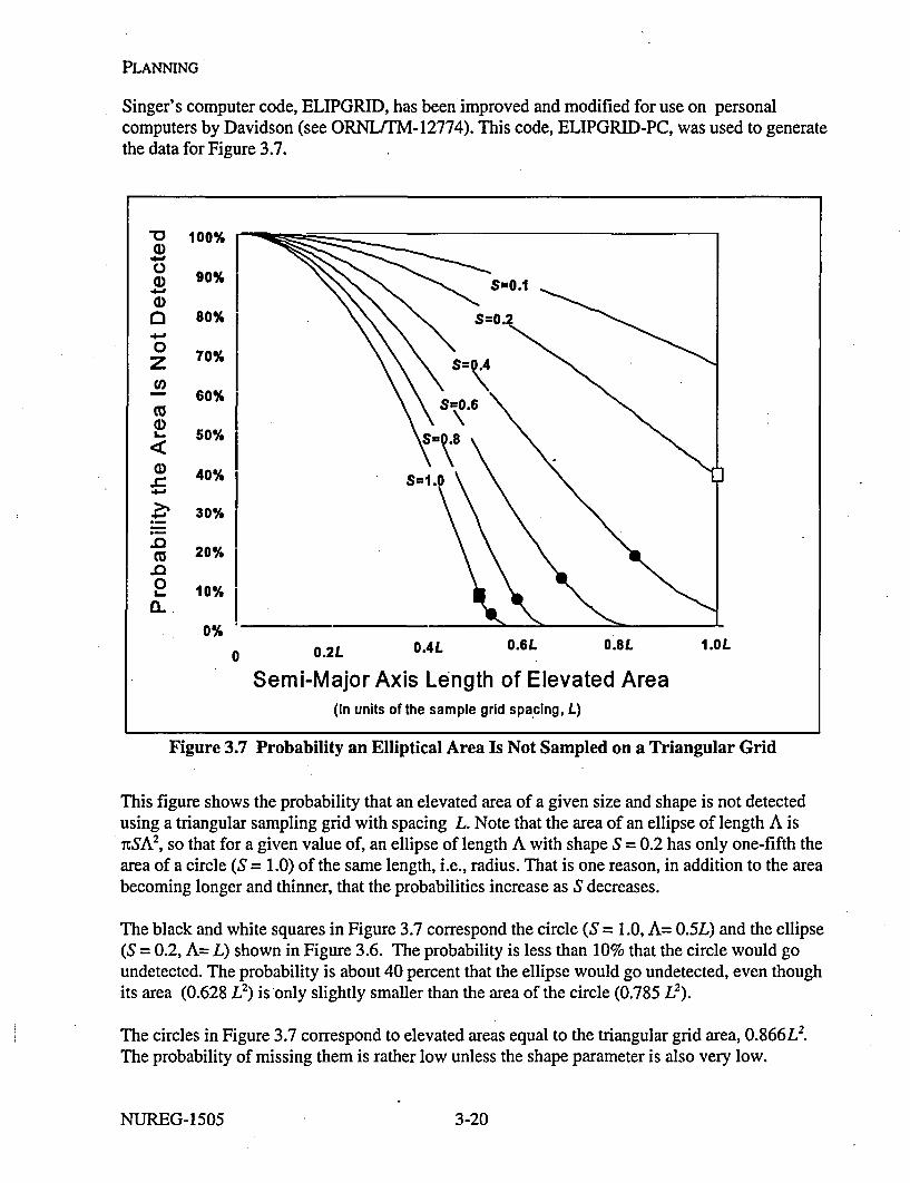
PLANNING
Singer's computer code, ELIPGRID, has been improved and modified for use on personalcomputers by Davidson (see ORNL/TM-12774). This code, ELIPGRID-PC, was used to generatethe data for Figure 3.7.
0)
4a)
.00)
100%
90%
80%
70%
60%
50%
40%
30%
20%
10%
0%
0 0.2L
Semi-Major0.4L 0.6L 0.8L
of Elevated Area
1.OL
Axis Length(In units of the sample grid spa~cing, L)
Figure 3.7 Probability an Elliptical Area Is Not Sampled on a Triangular Grid
This figure shows the probability that an elevated area of a given size and shape is not detectedusing a triangular sampling grid with spacing L. Note that the area of an ellipse of length A isnSA2, so that for a given value of, an ellipse of length A with shape S = 0.2 has only one-fifth thearea of a circle (S = 1.0) of the same length, i.e., radius. That is one reason, in addition to the areabecoming longer and thinner, that the probabilities increase as S decreases.
The black and white squares in Figure 3.7 correspond the circle (S = 1.0, A= 0.5L) and the ellipse(S = 0.2, A= L) shown in Figure 3.6. The probability is less than 10% that the circle would goundetected. The probability is about 40 percent that the ellipse would go undetected, even thoughits area (0.628 L2) is only slightly smaller than the area of the circle (0.785 L2).
The circles in Figure 3.7 correspond to elevated areas equal to the triangular grid area, 0.866L2.The probability of missing them is rather low unless the shape parameter is also very low.
NUREG-1505 3-20

PLANNING
In Figure 3.8, the probabilities of missing a circular elevated area with triangular and squaresystematic grids are compared. The square grid is only slightly less efficient than the triangulargrid. It can be concluded that, in most cases, an elevated area of the same size as, or larger than,that defined by the sampling grid is likely to be discovered during the final status survey.
0.9 ¾
* 0.8 . . Square
0 \J .. . ." Triangular
4 0.7to
00.0.5
0.4
0
*~0.2
r~0.1
00 0.1L 0.2L 0.3L O.4L 0.5L 0.6L 0.7L
Radius of Circular Area (in units of grid spacing, L)
Figure 3.8 Probability a Circular Area Is Not Sampled on a Systematic Grid
3.8 Optimize the Design
The DQO process need be neither static nor sequential. Some of the activities involved may betaking place concurrently, and may be visited more than once. At any stage in the process, newinformation may be available that should then be incorporated into planning the final statussurveys.
Optimization of the final status survey involves examining all of the factors that effect thedecision errors and sample sizes so that costs and potential risks are balanced. The primaryfactors to be considered in optimizing the design for determining the mean concentration are theDCGLw and the measurement standard deviation. The estimate of the measurement standarddeviation should include both the uncertainty in measurement process and any anticipated spatialand temporal concentration variations. The delineation and classification of survey units andreference areas can affect the spatial variability. Scan sensitivity is a primary consideration inoptimizing the design to ensure no elevated areas remain in a survey unit. The Area Factor and
3-21 NUREG-1505

PLANNING
the scan MDC are the important parameters which can impact survey costs and uncertainty.
3.8.1 Optimizing the Design for the Mean Concentration
There are relationships between the measurement uncertainty, a, the width of the gray region, A,the desired decision error limits (a and P3) and the number of measurements needed to meetthose limits. This is illustrated in Table 3.2 for the case when no reference area is needed (one-sample test). Table 3.3 is used when the survey unit is compared to a reference area (two-sampletest), and lists the number of samples to be taken in each. The method used to generate thesetables is discussed in Chapter 9.
Table 3.2 Number of Samples, N, Required in Survey Unit to Meet Error Rates ac, and ,With Relative Shift A/a, When Using the Sign Test
o=0.1cc =0.05 a = 0.10 a = 0.25
A/ay 0.01 0.05 0.10 0.25 0.01 0.05 0.10 0.25 0.01 0.05~ 0.10 0.25 0.01 0.05 0.10 0.250.1 4095 2984 2463 1704 2984 2048 1620 1018 2463 1620 1244 725 1704 1018 725 3450.2 1035 754 623 431 754 518 410 258 623 410 315 184 431 258. 184 88
0.3 468 341 282 195 341 234 185 117 282 185 143 83 195 117 83 40
0.4 270 197 162 113 197 136 107 68 162 107 82 48 113 68 48 230.5 178 130 107 75 130 89 71 45 107 71 54 33 75 45 33 160.6 129 94 77 54 94 65 52 33 77 52 40 23 54 33 23 110.7 99 72 59 41 72 50 40 26 59 40 30 18 41 26 18 90.8 80 58 48 34 58 4032 21 48 32 24 1534 2115 80.9 66 48 40 28 48 34 27 17 40 27 21 12 28 17 12 61.0 57 41 34 24 41 29 23 15 34 23 18 11 24 15 11 5
1.1 50 36 3021 36 2621 1430 2116 1021 1410 51.2 45 33 27 20 33 23 18 12 27 18 15 9 20 12 9 5
1.3 41 30 26 17 30 21 17 11 26 17 14 8 17 11 8 4
1.4 38 28 23 16 28 20 16 10 23 16 12 8 16 10 8 4
1.5 35 27 22 15 27 18 15 10 22 15 11 8 15 10 8 4
1.6 34 24 21 15 24 17 14 9 21 14 11 6 15 9 6 4
1.7 33 24 20 14 24 17 14 9 20 14 10 6 14 9 6 4
1.8 32 23 20 14 23 16 12 9 20 12 10 6 14 9 6 4
1.9 30 22 18 14 22 16 12 9 18 12. 10 6 14 9 6 4
2.0 29 22 18 12 22 15 12 8 18 12 10 6 12 8 6 3
3.0]2720 1712120 14.11 8117 11 9 5112 8 5 3I
NUREG- 1505 323-22

PLANNING
Table 3.3 Number of Samples, N12, Required in Both Reference Area and Survey Unit toMeet Error Rates a and P3 With Relative Shift A/o, When Using the WilcoxonRank Sum Test
a = 0.01 a = 0.05 cc = 0.10 a = 0.25
A/a 0.01 0.05 0.10 0.25 0.01 0.05 0.10 0.25 0.01 0.05 0.10 0.25 0.01 0.05 0.10 0.25
0.1
0.2
0.3
0.4
0.5
5452 3972 3278 2268
1370 998 824 570
614 448 370 256
350 255 211 146
227 .166 137 95
3972 2726 2157 1355
998' 685 542 341
3278 2157 1655 964
824 542 416 243
2268 1355 964 45c
570 341 243 11(
448 307 243 1531 370 243 187 1091 256 153 109
255 175 139 871 211 139 106
0.6
0.7
0.8
0.9
1.0
1.1
1.2
1.3
1.4
1.5
1.6
1.7
1.8
1.9
2.0
2.25
2.5
2.75
3.0
3.5
4.0
161
121
95
77
64
55
48
43
38
35
32
30
28
26
25
22
21
20
19
18
18
117
88
69
56
47
40
35
31
28
25
23
22
20
19
18
16
15
15
14
13
13
97
73
57
47
39
33
29
26
23
21
19
18
17
16
15
14
13
12
12
11
11
67
51
40
32
27
23
20
18
16
15
14
13
12
11
11
10
9
9
8
8
8
166 .114
117 81
88 61
69 48
56 39
47 32
40 28
35 24
31 22
28 19
25 18
23 16
22 15
20 14
19 13
18 13
16 11
15 11
15 10
14 10
13 9
13 9
90 57
64 40
48 30
38 24
31 20
26 16
22 14
19 12
17 11
15 10
14 9
13 8
12 8
11 7,
11 7
10 7
9 6
9 6
8 5
8 5
8 5
7 5
137
97
73
57
47
39
33
29
26
23
21
19
18
17
16
15
14
13
12
12
11
11
90 69
64 49
48 37
38 29
31 24
26 20
22 17
19 -15
17 13
15 12
14 11
13 10
12 9
11 9
11 8
10 8
9 7
9 7
8 6
8 6
8 6
7 6
62
41
29
22
17
14
12
10
9
8
7
7
6
6
5
5
5
4
4
4
4
4
4
146
95
67
51
40
32
27
23
20
18
16
15
14
13
12
11
11
10
9
9
8
8
8
87
57
40
30
24
20
16
14
12
11
10
9
8
8
7
7
7
6
6
5
5
5
5
62
41
29
22
17
14
12
10
9
8
7
7
6
6
5
5
5
4
4
4
4
4
4
The width of the gray region, A, is a parameter that is central to the nonparametric tests discussedin this report. It is also referred to as the shift. In this report, the gray region is always boundedfrom above by the DCGLw corresponding to the release criterion. The Lower Boundary of the
3-23 NUREG-1505

PLANNING
Gray Region (LBGR) is selected during the DQO process along With the target values for a and3, as discussed in Section 3.7.1. The width of the gray region, or shift, A, is equal to (DCGL -
LBGR). The absolute size of the shift is actually of less importance than the relative shift A/a,where a is an estimate of the standard deviation of the measured values in the survey unit. Theestimated standard deviation, a, includes both the real spatial variability in the quantity beingmeasured, and the precision of the chosen measurement method. The relative shift, A/o, is an,expression of the resolution of the measurements in units of measurement uncertainty.Expressed in this way, it is easy to see that relative shifts of less than one standard deviation, A/a< 1, will be difficult to detect. On the other hand, relative shifts of more than three standarddeviations, A/a > 3, are generally easy to detect.
It is evident from Tables 3.2 and 3.3, that the number of measurements that will be required toachieve given error rates (a and P3) depends entirely on the value of A/a. Note also that thenumber of measurements required is symmetric in a and 3. For example, if A/a =1, cc = 0.05 andP3 = 0.10, then, from Table 3.1, the number of samples needed for the Sign test is 23. For thesame value of A/a, but with error rates reversed (i.e., a = 0.10 and 13 = 0.05), the number of.samples needed for the Sign test is again 23. Thus, these tables may be used to plan the numberof measurements needed, regardless of whether Scenario A or Scenario B is used. It is only whenthe statistical test is actually performed on the measurement results that the distinction betweena and P3 becomes important.
For fixed values of a and 13, small values of A/a result in large numbers of samples. It isdesirable to design for A/a > 1 whenever possible. There are two obvious ways to increase A/a.The first is to increase the width of the gray region by making LBGR small. The disadvantage isthat the acceptable probability of the survey unit passing will be specified at this smaller LBGR.Thus, a survey unit will generally have to be lower in residual radioactivity to have a highprobability of being judged to meet the release criterion. The second way to increase A/c is to,make a smaller. One way to make a small is by having survey units that are relativelyhomogeneous in the amount of measured radioactivity. This is an important consideration inselecting survey units that have both relatively uniform levels of residual radioactivity and alsohave relatively uniform background radiation levels. Measurements performed during scoping,characterization, and remedial action support surveys can be useful for determining an estimateof a for the final status survey planning.
Another way to make a small is by using more precise measurement methods. The more precisemethods might be more expensive, but this may be compensated for by the decrease in thenumber of required measurements. One example would be in using a radionuclide specificmethod rather than gross radioactivity measurements for residual radioactivity that does notappear in background. This would eliminate the variability in background from a, and wouldalso eliminate the need for reference area measurements. On the other hand, the costs associatedwith performing additional measurements with an inexpensive measurement system may be lessthan the costs associated with fewer measurements of higher precision.
The effect of changing the width of the gray region and/or changing the measurement variabilityon the estimated number of measurements (and cost) can be investigated using Table 3.1 and 3.2.Generally, the design goal should be to achieve A/a values between one and three. ' The numberof samples needed rises dramatically when A/a is smaller than one. Conversely, little is usually
NUREG-1505 3-24
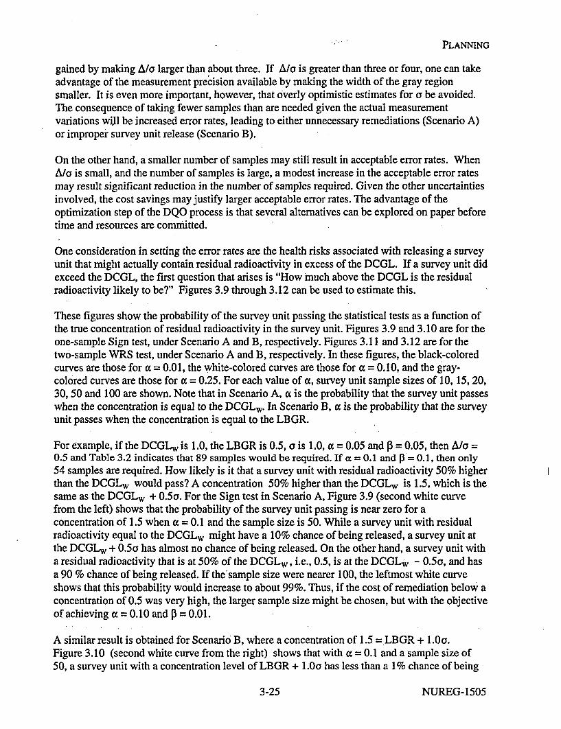
PLANNING
gained by making A/c larger than about three. If A/c is greater than three or four, one can takeadvantage of the measurement precision available by making the width of the gray regionsmaller. It is even more important, however, that overly optimistic estimates for a be avoided.The consequence of taking fewer samples than are needed given the actual measurementvariations will be increased error rates, leading to either unnecessary remediations (Scenario A)or improper survey unit release (Scenario B).
On the other hand, a smaller number of samples may still result in acceptable error rates. WhenA/a is small, and the number of samples is large, a modest increase in the acceptable error ratesmay result significant reduction in the number of samples required. Given the other uncertaintiesinvolved, the cost savings may justify larger acceptable error rates. The advantage of theoptimization step of the DQO process is that several alternatives can be explored on paper beforetime and resources are committed.
One consideration in setting the error rates are the health risks associated with releasing a surveyunit that might actually contain residual radioactivity in excess of the DCGL. If a survey unit didexceed the DCGL, the first question that arises is "How much above the DCGL is the residualradioactivity likely to be?" Figures 3.9 through 3.12 can be used to estimate this.
These figures show the probability of the survey unit passing the statistical tests as a function ofthe true concentration of residual radioactivity in the survey unit. Figures 3.9 and 3.10 are for theone-sample Sign test, under Scenario A and B, respectively. Figures 3.11 and 3.12 are for thetwo-sample WRS test, under Scenario A and B, respectively. In these figures, the black-coloredcurves are those for ac = 0.01, the white-colored curves are those for a = 0.10, and the gray-colored Curves are those for a = 0.25. For each value of a, survey unit sample sizes of 10, 15, 20,30, 50 and 100 are shown. Note that in Scenario A, a is the probability that the survey unit passeswhen the concentration is equal to the DCGLw. In Scenario B, a is the probability that the surveyunit passes when the concentration is equal to the LBGR.
For example, if the DCGLw is 1.0, the LBGR is 0.5, a is 1.0, a = 0.05 and 3 = 0.05, then A/a =0.5 and Table 3.2 indicates that 89 samples would be required. If cc = 0.1 and P3= 0.1, then only54 samples are required. How likely is it that a survey unit with residual radioactivity 50% higherthan the DCGLw would pass? A concentration 50% higher than the DCGLw is 1.5, which is thesame as the DCGLw + 0.5a. For the Sign test in Scenario A, Figure 3.9 (second white curvefrom the left) shows that the probability of the survey unit passing is near zero for aconcentration of 1.5 when a = 0.1 and the sample size is 50. While a survey unit with residualradioactivity equal to the DCGLw might have a 10% chance of being released, a survey unit atthe DCGLw + 0.5a has almost no chance of being released. On the other hand, a survey unit witha residual radioactivity that is at 50% of the DCGLw, i.e., 0.5, is at the DCGLW - 0.5a, and hasa 90 % chance of being released. If the'sample size were nearer 100, the leftmost white curveshows that this probability would increase to about 99%. Thus, if the cost of remediation below aconcentration of 0.5 was very high, the larger sample size might be chosen, but with the objectiveof achieving a = 0.10 and P = 0.01.
A similar result is obtained for Scenario B, where a concentration of 1.5 =LBGR + 1.0o.Figure 3.10 (second white curve from the right) shows that with a = 0.1 and a sample size of50, a survey unit with a concentration level of LBGR + 1.0Oa has less than a 1% chance of being
3-25 NUREG-1505
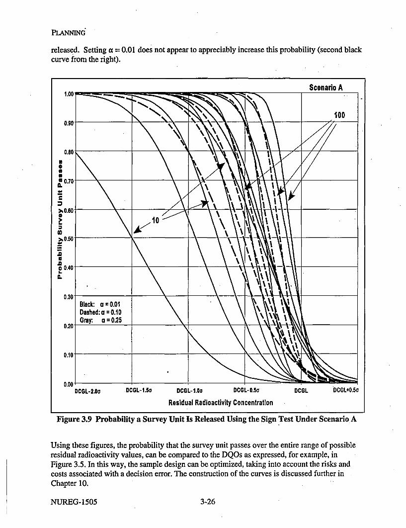
PLANNINd
released. Setting a = 0.01 does not appear to appreciably increase this probability (second blackcurve from the right).
Scenario A
Cn>b
N
0
0.600
0.40
0.30
03-Bla ck: a=0.01Dashed: a =0.10
0 0 -Gray: a 0 .25N
0.20
DCGL-2.0a DCGL-1.5o DCGL-A.No DCOL-O.5o DCGL DCGL+0.5a
Residual Radioactivity Concentration
Figure 3.9 Probability a Survey Unit Is Released Using the Sign Test Under Scenario A
Using these figures, the probability that the survey unit passes over the entire range of possibleresidual radioactivity values, can be compared to the DQOs as expressed, for example, inFigure 3.5. In this way, the sample design can be optimized, taking into account the risks andcosts associated with a decision error. The construction of the curves is discussed further inChapter 10.
NUREG-1505 3-26

PLANNING
Scenario B1.fn n. I I
~zcj
UIIUIA.
I
(0
.0U.001~A.
0.70,V
~0.60-
~0.50
0.40
0.30-Black: a 0.01Dashed: a 0.10Gray: a 0.25
0.20Z___
0.10
U.1WULBGR-0.5a LBGR LBGR+0.5a LBGR+ ai.O n LBGR+1.5a LBGR+2.Oa
Residual Radioactivity Concentration
Figure 3.10 Probability a Survey Unit Is Released Using the Sign Test Under Scenario B
3.8.2 Optimizing the Design for Detecting Elevated Areasi
As discussed in Section 2.2, one objective of the final status survey is to provide reasonableassurance that there are no small areas of elevated residual radioactivity left within the surveyunit that might cause the release criterion to be exceeded. However, it is inefficient to treat allsurvey units equally in this regard. During the process of survey unit classification, Class 1survey units are identified as those with the potential for such elevated areas. Measurements and
3 -27 NUREG-1505

PLANNING
sampling on a systematic grid, in conjunction with scanning, are used to assure that any smallareas of elevated radioactivity that might remain within a Class 1 survey units will not produce adose in excess of the release criterion. To accomplish this, an additional step in the survey designoptimization is required.
Scenario A
C
N
0L.IL
1.000
0.90 r
0.80-
I0.70 _ ____ _________
10
*0.60'
0.50-
0.40-
0.30- X -Black: a 0.01Dashed: a =0.10
0.20 -________
U.1U
.UXuDCGL-2.0o DCGL-t.5a RduL-.aoa DCGL-O.5o DCGL DCGL4O.5a
Residual Radioactivity Concentration
Figure 3.11 Probability a Survey Unit Is Released Using WRS Test Under Scenario A
The number of samples, N, to be taken on a random start systematic grid in a survey unit of areaA, determines the spacing, L, between the samples (see Section 3.4.5). Corresponding to thisspacing is the grid area delimited by neighboring sampling locations. This grid area is 0.866 L2
for a triangular grid and L' for a square grid.
NUREG-1505 3-28

PLANNING
Scenario BI nn I I
~ZZN
0
1.4L
0.801100--
0.70 -
0.60,
0.50o
0.40
0.30Black: a 0.01Dashed: a = 0.10Gray: a 0.25
0.201
0.10.
f i f
LBGR-0.5a LBGR LBGR+0.5o LBGR.1.Oa LBGR1.5aS LBGR+2.Oo
Residual Radioactivity Concentration
Figure 3.12 Probability a Survey Unit Is Released Using WRS Test Under Scenario B
A given concentration of residual radioactivity spread over a smaller area will, in general, resultin a smaller dose. Thus, the DCGLEMc used for the elevated measurement comparison is usuallylarger than the DCGLw used for the statistical test. The amount of residual radioactivity thatwould have to exist within the grid area between sampling locations in order to exceed theguideline dose is a multiple, FA, of the residual radioactivity derived concentration guidelinelevel, DCGLw. Values for the area factor, FA, can be determined by comparing the doseconversion factor (DCF) obtained from the results of a pathway analysis under the scenario that aunit activity concentration of a given radionuclide is distributed uniformly across the survey unit
3 -29 NUREG-1505

PLANNING
to the DCF obtained when a unit concentration of that radionuclide is confined to the smaller gridarea. For some radionuclides, especially those that deliver dose primarily via internal pathways,the dose is approximately proportional to inventory, and so the ratio of the DCGLEmc to theDCGLw is nearly proportional to the ratio of the survey unit area to the grid area. However, thismay not be the case for radionuclides that deliver a significant portion of the dose via externalexposure. The exact relationship between the DCGLEmc and the DCGLw is generally acomplicated function of the dose modeling pathways.
The scanning procedure used for the survey unit should have a minimum detectableconcentration (MDC) less than the DCGLEMc. The DCGLEMc depends on the grid area which inturn depends on the spacing of the samples. Once a scanning technique is selected, the actualMDC can be compared to the DCGLEMC. If the actual scan MDC is less than the DCGLEMC, thesurvey design is complete. When the scanning method is sensitive enough to detect residualradioactivity concentrations at the DCGLEMC, the combination of sampling and scanning will besufficient to provide reasonable assurance that release criterion is met by any residualradioactivity remaining in the survey unit. Any area smaller than the grid area would require aresidual radioactivity concentration within it larger than DCGLEMc = (FA)(DCGLw) in order toexceed the release criterion. Recall from the discussion in Section 3.7.2 that any area larger thanthe grid area is likely to be hit by a sampling location on the systematic grid at least once.
If the scanning MDC is greater than the DCGLEMO then the survey design must be modified. Alarger DCGLEMc is generally obtained by decreasing the sampling grid area, i.e., adding moresampling locations to the grid. The number of additional sampling locations can be found bydetermining the area factor necessary to raise the DCGLEMC to a level detectable by scanning:
FA = (Scan MDC) / (DCGLw).
The sampling grid area, AuMc, that corresponds to this area factor can be used to determine thesample size for the survey unit. Dividing the survey unit area, As, by the revised sampling gridarea AuDc yields the required sample size, nut* = As IAuDc.
Thus, for Class 1 Survey Units, the number of samples may be driven more by the need to detectsmall areas of elevated activity than by the requirements of the statistical tests. This in turn willdepend primarily on the sensitivity of available scanning instrumentation, the size of the area ofelevated activity, and the dose model. For many radionuclides, scanning instrumentation isreadily available that is sensitive enough to detect residual radioactivity concentrations at theDCGLEmc derived for the sampling grid of direct measurements used in the statistical tests.Where instrumentation of sufficient sensitivity is not available, the number of samples in thesurvey unit can be increased until the area between sampling points is small enough (and theresulting area factor is large enough) that DCGLEMC can be detected by scanning. For someradionuclides (e.g., 311), the scanning sensitivity is so low that this process would neverterminate-i.e., the number of samples required could increase without limit. Thus, an importantpart of the DQO process is to determine the smallest size of an area of elevated activity that it isimportant to detect, Amn, and an acceptable level of risk, RPA , that it may go undetected. Figures3.7 and 3.8 can be used for this purpose. The ELIPGRID-PC computer code (ORNL/TM-12774,1994) can also be used to calculate these risks.
NUREG-1505 3-30

PLANNING
In this part of the DQO process, the concern is less with areas of elevated activity that are foundthan with providing adequate assurance that negative scanning results truly demonstrate theabsence of such areas. In selecting acceptable values for A ,m and RA, maximum use ofinformation from the historical site assessment and all surveys prior to the final status surveyshould be used to determine what sort of areas of elevated activity could possibly exist, theirpotential size and shape, and how likely they are to exist.
3-31 NUREG-1505


4 ANALYSIS OF FINAL STATUS SURVEY RESULTS:DATA QUALITY ASSESSMENT
Data Quality Assessment (DQA) is the scientific and statistical evaluation of data to determine ifthe data are of the right type, quality, and quantity to support their intended use (EPA QA/G-9,1995). There are five steps in the DQA process:
(1) Review the Data Quality Objectives (DQOs).and sampling design.(2) Conduct a preliminary data review.(3) Select the statistical test.(4) Verify the assumptions of the statistical test.(5) Draw conclusions from the data.
4.1 Review the Data Quality Objectives (DQOs) and Sampling Design
During survey design, acceptable error rates are specified for the statistical tests; and the desiredprobability that a survey unit will pass the release criterion is charted against the amount ofresidual radioactivity that actually may be present in order to test the efficacy of a proposeddesign. During the interpretation of survey results, it is important to determine that the objectivesof the design have been met. The first and most straightforward way to check this is to ascertainthat the number of usable measurements meet the requirement of the statistical tests as outlinedin Section 3.8.1. The sample standard deviation, s, should also be compared to the estimate of themeasurement variability, a, that was used to determine the number of samples required. Theconsequence of there being too few measurements, or of there being higher than expected datavariability, is that the Type II error rate P3 will be larger than planned, and the power of the test todetect departures from the null hypothesis, 1 - 3, is reduced. In Scenario A this means that asurvey unit that meets the release criterion has a higher probability of being incorrectly deemednot to meet it. In Scenario B this means that a survey unit that does not meet the release criterionhas a higher probability of being incorrectly deemed to meet it. After examining the number ofusable measurements and their variability, the retrospective power of the test can be determinedusing the methods of Chapter 10. This is not usually necessary when the null hypothesis isrejected since the Type I error rate, co, is fixed when the statistical test is performed using theactual number of usable measurements.
Since the occurrence of missing or unusable data can impact the Type II error rates, a reasonableallowance for such occurrences should be built into the planning process by adding moremeasurements to the sample sizes listed in Tables 3.2 and 3.3.
The power of the statistical tests will'also be reduced if data variability is greater than thatassumed during the survey planning. The number of measurements required to meet theacceptable error specified during the planning process will not be sufficient if a wasunderestimated. As mentioned in Section 2.2.6, the overall data variability may be considered toconsist of two more or less independent components, the component due to uncertainty in themeasurement process, measn and the component due to spacial variability in the concentrations
4-1 NUREG-1505

ANALYSIS
being measured, ospatial, Spatial variability was discussed in Section 3.5.1. The overall variability
is approximately a = 0mes2 + Ospatial2. If either standard deviation is one-third or less of the
other, there is not much point in trying to reduce it further. If the smaller contributor were
eliminated entirely, at most a would be reduced by a factor of 01/910-0.95, i.e., only about a
5% gain. Efforts should be directed at reducing the dominant component of the data variability.
The quality of data is critical to the successful execution of a survey. Even if the measurementuncertainty is dominated by the spatial variability, poorly calibrated instruments could lead toeither improperly labeling an area as still contaminated or releasing it when, in fact, it is abovethe guidelines. For this reason, calibrations must be performed regularly with traceablestandards; the inherent precision of the survey instrument must be evaluated to determine if itmeets the needs of the survey plan. Energy responses of instruments must be known so thatappropriate applications are made to different radiation fields. Replicate, reference, and blankmeasurements are also an integral part of the survey methodology. Comparisons of fieldmeasurement results to those of laboratory sample analyses forms an important quality controlcheck.
Bounds on measurement uncertainties should be established in the planning process and regularlyassessed throughout the measurement program. Uncertainties in the measurements add to thevariance in distribution of data sets and should be taken into consideration when selectingparameters for the statistical tests and in the interpretation of results of these tests. Failure toadequately consider the effect of measurement errors could result in the added expense ofadditional measurements. In the worst case, inadequate control of the Type II statistical errors asdetermined from a retrospective power calculation, could invalidate the final survey results andrequire a re-survey. For this reason, it is better to plan the surveys cautiously:
" It is better to overestimate the potential data variability than to underestimate it.
* It is better to take too many samples than too few.
* It is better to overestimate minimum detectable concefitrations (MDCs) than to underestimatethem.
Further information on quality assurance for environmental data may be found in EPA QA/R-5(1994), EPA QA/G-5 (1996), and ANSI/ASQC (1994)
4.2 Conduct a Preliminary Data Review
To learn about the structure of the data-identifying patterns, relationships, or potentialanomalies-one can review quality assurance (QA) and quality control (QC) reports, preparegraphs of the data, and calculate basic statistical quantities.
Radiological survey data are usually obtained in units that have no intrinsic meaning relative toDCGLs, such as the number of counts per unit time. For comparison of survey data to DCGLs,
NUREG-1505 4-2

ANALYSIS
the survey data from field and laboratory measurements should be converted to DCGL units.
4.2.1 Basic Statistical Quantities
Basic statistical quantities that should be calculated for the sample data set are the" mean" standard deviation* median
The average of the data can be compared to the reference area average and the DCGL wto get apreliminary indication of the survey unit status. Where remediation is inadequate, thiscomparison may readily reveal that a survey unit contains excess residual radioactivity-evenbefore applying statistical tests. For example, if the average of the data exceeds the DCGL wandthe radionuclide of interest does not appear in background, then it is obvious that the survey unitdoes not meet the release criterion. On the other hand, if every measurement in the survey unit isbelow the DCGLw, the survey unit will always pass the Sign test.
The value of the sample standard deviation is especially important. If too large compared to thatassumed during the survey design, this may indicate an insufficient number of samples werecollected to achieve the desired test power.
The median is the middle value of the data set when the number of data points is odd, and is theaverage of the two middle values when the number of data points is even. Thus 50% of the datapoints are above the median, and 50% are below the median. Large differences between themean and the median would be an early indication of skewness in the data. This would also beevident in a histogram of the data.
Table 4.1 lists an example of concentration data taken in a reference area and survey unit. Forthis example, the quantity and units of measurement have been left arbitrary. Basic statisticalquantities can be calculated simply by using one of the many widely available personal computerprograms that perform data analysis. Table 4.2 shows the result of a "descriptive statistics"command applied to the data of Table 4.1 using a spreadsheet program. In addition to the mean,median and standard deviation, this table lists several other useful parameters such as theminimum, maximum, mode, range, skewness and kurtosis.
For the example survey unit, the mean is 1.15 and the median is 1.05. The sample standarddeviation is 0.46. The difference between the median and the mean, divided by the samplestandard deviation is sometimes used as a simple measure of skewness. In this case,(1.15 -1.05)/0.46 = 0.22.
The coefficient of skewness is the average cubed difference from the mean divided by the
standard deviation cubed. The sample estimate of skewness is g1 = M3 /m2 , where
n n n
m 3 = ,(xi-x) 3In , and m2 = • (x,-x) 2/n. m= m (xj-x) 2In.i=1 i=1 i=1
4-3 NUREG-1505

ANALYSIS
For a sample from a normal distribution, g, is approximately normal with mean zero and
standard deviation ý61n The sample skewness for the survey unit data is 0.96. This is nearly
four times VI-619 0 0.26, indicating that there is some positive skewness in this data set.
Table 4.1 Example Final Status Survey Data
___- Reference Area - Survey Unit- -_ _
Point Data Point Data Point Data Point Data Point Data Point DataNo. Value No. Value No. Value No. Value No. Value No. Value
1 1.1 31 1.9 61 0.8 91 1.2 121 0.7 151 0.82 1.3 32 1 62 1.1 92 1.4 122 1.9 152 1.13 0.7 33 0.7 63 0.6 93 0.8 123 1.3 153 1.24 0.7 34 1.9 64 0.8 94 0.6 124 1.4 154 0.75 1.6 35 1.0 65 1.2 ___ 95 1.4 125 0.5 155 1.46 1.0 36 0.6 66 0.8 96 2.9 126 1.0 156 1.67 1.1 37 1.5 67 1.0 97 0.9 127 1.3 157 0.48 0.7 .38 1.1 68 0.9 98 0.8 128 0.6 158 0.69 0.9 39 0.9 69 1.5 ___ 99 0.8 129 1.3 159 1.610 1.8 40 0.9 70 0.8 ___100 1.6 130 1.5 160 0.711 0.9 41 0.8 71 1.2 ___101 1.6 131 1.4 161 1.012 0.7 42 1.1 72 1.1 ___102 1.2 132 1.3 162 1.013 1.1 43 0.9 73 0.6 __ 103 1.2 133 0.8 163 1.814 1.1 44 1.2 74 1.0 ___104 2.5 134 1.5 164 1.315 0.9 45 1.2 75 0.9 __ 105 1.9 135 0.8 165 1.516 1.5 46 1.0 76 1.0 ___106 1.9 136 1.1 166 0.817 1.0 47 1.3 77 0.6 ___107 0.9 137 1.1 167 1.518 0.8 48 0.9 78 0.9 ___108 0.9 138 1.0 168 0.919. 0.6 49 0.8 79 1.0 ___109 0.8 139 1.1 169 0.920 1.1 50 1.7 80 0.8 ___110 1.0 140 1.6 170 0.821 0.7 51 0.7 81 0.6 Ill_11 1.7 141 1.5 171 1.522 0.6 52 1.0 82 1.2 ___112 1.5 142 0.8 172 1.023 0.9 53 0.8 83 1.2 ___113 2.1 143 0.7 173 0.724 0.6 54 1.0 184 1.3 ___114 2.0 144 0.6 174 1.125 1.5 55 0.5 85 1.0 115 1.7 145 0.9 175 1.4
26 0.9 56 1.1 86 0.9 ___116 0.7 146 0.8 176 1.027 1.5 57 1.1 87 0.7 ___117 1.0 147 0.5 177 1.2
28 0.8 58 0.9 188 10.9 1__ .118 1.0 148 0.6 178 0.5
"29 1.1 59 0.9 189 1.4 ___119 1.5 149 0.8 179 0.53 1.2 60 0.6 190 1 __ 120 1 150 10.8 180 1.7
NUREG- 150544 4-4

ANALYSIS
Table 4.2 Basic Statistical Quantities Calculated for the Data in Table 4.1
Reference Survey Unit
Mean 1.00 Mean 1.15
Standard 0.03 Standard 0.05Error Error
Median 1.00 Median 1.05Mode 0.90 Mode 0.80
Standard 0.30 Standard 0.46Deviation Deviation
Sample 0.09 Sample 0.22Variance Variance
Kurtosis 0.93 Kurtosis 1.44
Skewness 0.95 Skewness 0.96
Range 1.4 Range 2.5
Minimum 0.5 Minimum 0.4Maximum 1.9 Maximum 2.9
Count 90 Count 90
The kurtosis is the average fourth power of the difference from the mean divided by the variancesquared. It is a measure of how "flat" the distribution is relative to normally distributed data. The
sample estimate of kurtosis is b2 = m 4 /M2 , where
nmn4 = •_ X-~~ , and
i=1in2 ~(Xi_ )2 In =(n_1)S2In.
For a sample from a normal distribution, b2 has mean three. The sample coefficient of kurtosis is92 = b2 - 3. For very large samples from a normal distribution, g2 has mean zero and standard
deviation ý2-44n (Snedecor and Cochran, 1980). The sample coefficient of kurtosis for the
survey unit data is 1.44, and .Thus, the kurtosis appears to be significantly greater than zero. It isan indicator of how well the sample variance, S2, estimates the true variance, o2, of themeasurement data. The variance of the sample estimate of the variance is
Var(s 2) = 2j4 [ + n-1 92 ]
The variance of s is given approximately by
4-5 NUREG-1505

ANALYSIS
Var(s) = Var(s 2) -L Var(s 2 ) 2 C14 [l+n-1 ] - s3 [Ln-1 ]1+4s 4s(n-1) 2•"'n g 2(n-l) 2n
where the propagation of error formula for the variance of the square root has been used (Taylor,1990). For the example survey unit data with s = 0.36, 92= 1.44, and n = 90, we have
Var(s) = (6.46)3 [1+ i-1.448 (0.0973/178)(1.712) =0.000936.2(89) 18
The standard deviation of s = V = •0.000936 = 0.0306. Thus, one can estimate that,
very roughly, s = 0.46 ± 0.03.
An approximate 1- a confidence interval for a2 may be obtained from
2_-,(x/f2) < [0 <(n -1)s2]/ _I+ g21n X" +92/n X ,
where Xn I (a) is the 100ath percentile of the chi-squared distribution with n-1 degrees of
freedom (Box, 1953). Percentiles of the chi-squared distribution are given in Table A.5. With
s2 = 0.22,92 =1.44, n = 90, X89(0.975) 117, and X89(0.025) = 64.8, we find that with 95%
confidence [ (•(0.22)' 117 < o< < 1(89)(022) 64.8 or 0.1647<a2<0.2974,
which implies that 0.406 < 0 < 0.545. This is not too different from the cruder estimates = 0.46 ± (2) (0.03) = 0.46 ± 0.06, using a 2o interval about the mean.
Examining the minimum, maximum, and range of the data may provide additional usefulinformation. The minimum of the example survey unit data is 0.4 and the maximum is 2.9, sothe range is 2.9 - 0.4 = 2.5. This is 5.4 times the standard deviation of 0.46. Figure 4.1 showsthat is well within the expected spread of values for this ratio, which is sometimes called thestudentized range. These intervals were calculated for normally distributed data.
Absolute upper and lower bounds for the studentized range have been found by Thomson (1955).
These bounds are fairly wide, but are useful in checking for errors in calculation. The upper
bound is j2(Qnl) . The lower bound is 2j(n-•)/n , when n is even, and 2VIn/(n+ 1) , when n
is odd.
NUREG-1505 4-6

ANALYSIS
80 7-a~6
L.0
/~0 00 oo' •,10 5
(U0
2.10 100 1000
Sample Size
Figure 4.1 Confidence Bands for the Ratio of the Range to the Standard DeviationDotted: 90% Dashed: 95% Solid: 99%
Transformations are sometimes used bring data closer to a normal distribution, and decrease anydependence of the variance on the mean. A rule of thumb sometimes used is that if the ratio ofthe data maximum to the data minimum is less than 20, no data transformation is necessary tostabilize the variance of the data (EPA 600/4-90/013, 1990). For the example survey unit data,this ratio is 2.9/0.4 = 7.25.
Many of the "diagnostic checks" on the basic statistical quantities discussed in this section arebased on comparing the values computed for the sample data distribution to those that would beexpected if the data were normally distributed. When viewed as tests of normality, they aregenerally not very powerful, and are not suggested here for that purpose. As noted earlier, thenonparametric statistical tests used in this report do not assume the data are normally distributed.Rather, these checks are being used as exploratory techniques to alert the data analyst of anyunusual features in the data.
4.2.2 Graphical Data Review
At a minimum, the graphical data review should consist of a posting plot and a histogram. Rankor Quantile plots are also useful diagnostic tools, particularly in the two-sample case, to comparethe survey unit and reference area.
4-7 NUREG-1505

ANALYSIS
A posting plot, which is simply a map of the survey unit with the data values entered at themeasurement locations, will reveal potential anomalies in the data, especially possible patches ofelevated residual radioactivity. Even in a reference area, a posting plot can reveal spatial trends inbackground data that might affect the results of the two-sample statistical tests.
The survey unit data in Table 4.1 were taken on a square systematic grid in a rectangular surveyunit. A simple posting plot is shown in the upper half of Figure 4.2. It is often useful to add somecolor coding of data values to aid in identifying patterns. In the lower half of Figure 4.2, darkershading was used for larger data values. The small slightly elevated region near 40 East and 20North stands out more clearly when the shading is added.
If the posting plot reveals systematic spatial trends in the survey unit, the cause would need to beinvestigated. In some cases, such trends could be due to residual radioactivity, but may also bedue to an inhomogeneous survey unit background. Other diagnostic tools for examining spatialdata trends may be found in EPA Report QA/G-9 (1996). Geostatistical tools may also be usefulin some cases (EPA 230/02-89-042, 1989a).
A frequency plot (or a histogram) is a useful tool for examining the general shape of a datadistribution. This plot is a bar chart of the number of data points within a certain range of values.The frequency plot will reveal any obvious departures from symmetry, such as skewness orbimodality (two peaks), in the data distributions for the survey unit or reference area. Skewnessor other asymmetry can impact the accuracy of the statistical tests. A data transformation (e.g.,taking the logs of the data) can sometimes be used to make the distribution more symmetric. Thestatistical tests could then be performed on the transformed data. The interpretation of the results,however, can be more complex, since the quantity being tested is also transformed. For example,
the mean of log-transformed data is the log of the geometric mean of the data, not the log of thearithmetic mean of the data.
The presence of two peaks in the survey unit frequency plot may indicate the existence ofisolated areas of residual radioactivity. In some cases it may be possible to determine anappropriate background for the survey unit using this information. The interpretation of the datafor this purpose will generally be highly dependent on site-specific considerations and shouldonly be pursued after consultation with the responsible regulatory agency.
The presence of two peaks in the reference area frequency plot may indicate a mixture ofbackground concentration distributions due to different soil types, construction materials, etc.The greater variability in the data due to the presence of such a mixture will reduce the power ofthe statistical tests to detect an adequately remediated survey unit. These situations should beavoided whenever possible by carefully matching the reference areas to the survey units, andchoosing survey units with homogeneous backgrounds.
A major concern in constructing a histogram or frequency plot is the bin width, i.e. the range ofconcentration values over which the data are grouped and counted. If the bin width is too narrow,there will be too much spurious detail in the plot. If the bin width is too wide, too much detail islost. A useful rule of thumb is to calculate the bin Width by rounding down the quantity 3.5sn" 3,
where n is the number of data points, and s is the sample standard deviation (Scott, 1979). Anexample is shown in Figure 4.3 using the example survey unit data. In this example,
NUREG-1505 4-8

ANALYSIS
3.5sn'"' = 3.5(0.46)(90)"'n = 3.5(0.32)(0.22) = 0.354, which was rounded down to 0.3. Theresulting histogram is shown as Figure 4.3a. For comparison, histograms constructed using binwidths of 0.2 (Figure 4.3b) and 0.1 (Figure 4.3c) are also shown.
Figure 4.2 Example of a Posting Plot
4-9 NUREG-1505

ANALYSIS
15-
10 I (c)
II I I5
0 III -[141 40 CO 4- N V eq CO CM C! -0 40 Cco; C C; V: V: VZ ~-r C4 C4 C4
20-
10-
(" ?-* W- V)0 t-C V- 0C) 0 40 0 V - W. V- %- W 4 N4 4 N4
(a)201
IU
5
0 IL" -1. ý, . JMIL-
0r.-40 I- V N N
Figure 4.3 Frequency Plots of Example Survey Unit Datawith bin width 0.1 (c-top) and 0.2 (b-middle) and 0.3 (a-bottom)
A ranked data plot indicates the amount of data falling within a given range of values. The firststep in constructing a ranked data plot is to sort the data in increasing order. The data are thenassigned the number corresponding to their position in the list. The ranking of the example datafrom Table 4.1 is shown in Table 4.3.
NUREG-1505 4-10
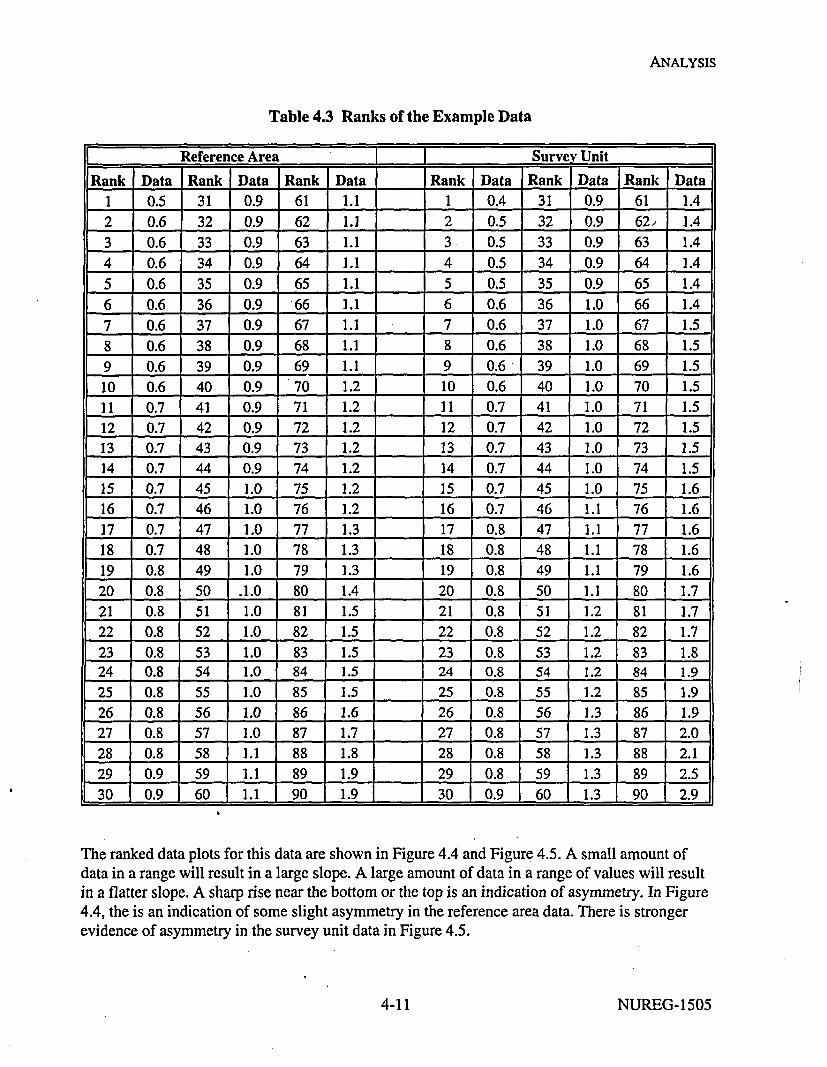
ANALYSIS
Table 4.3 Ranks of the Example Data
F - Reference Area ______I___I___-__ Survey Unit
Rank Data Rank Data Rank Data Rank Data Rank Data Rank Data
1 0.5 31 0.9 61 1.1 __ 1 0.4 31 0.9 61 1.4
2 0.6 32 0.9 62 1.1 2 0.5 32 0.9 62, 1.4
3 0.6 33 0.9 63 1.1 __ 3 0.5 33 0.9 63 1.4
4 0.6 34 0.9 64 1. 4 0.5 34 0.9 64 1.4
5 0.6 35 0.9 65 1.1 5 0.5 35 0.9 65 1.4
6 0.6 36 0.9 66 1.1 6 0.6 36 1.0 66 1.4
7 0.6 37 0.9 67 1.1 7 0.6 37 1.0 67 1.5
8 0.6 38 0.9 68 1.1 8 0.6 38 1.0 68 1.5
9 0.6 39 0.9 69 1.1 9 0.6 39 1.0 69 1.5
10 0.6 40 0.9 '70 1.2 10 0.6 40 1.0 70 1.5
11 0.7 41 0.9 71 1.2 11 0.7 41 1.0 71 1.5
12 0.7 42 0.9 72 1.2 12 0.7 42 1.0 72 1.5
13 0.7 43 0.9 73 1.2 13 0.7 43 1.0 73 1.5
14 0.7 44 0.9 74 1.2 14 0.7 44 1.0 74 1.5
15 0.7 45 1.0 75 1.2 15 0.7 45 1.0 75 1.6
16 0.7 46 1.0 76 1.2 16 0.7 46 1.1 76 1.6
17 0.7 47 1.0 77 1.3 17 0.8 47 1.1 77 1.6
18 0.7 48 1.0 78 1.3 18 0.8 48 1.1 78 1.6
19 0.8 49 1.0 79 1.3 19 0.8 49 1.1 79 1.6
20 0.8 50 .1.0 80 1.4 20 0.8 50 1.1 80 1.7
21 0.8 51 1.0 81 1.5 21 0.8 51 1.2 81 1.7
22 0.8 52 1.0 82 1.5 __ 22 0.8 52 1.2 82 1.7
23 0.8 53 1.0 83 1.5 23 0.8 53 1.2 83 1.8
24 0.8 54 1.0 84 1.5 24 0.8 54 1.2 84 1.9
25 0.8 55 1.0 85 1.5 25 0.8 55 1.2 85 1.9
26 0.8 56 1.0 86 1.6 26 0.8 56 -1.3 86 1.9
27 0.8 57 1.0 87 1.7 27 0.8 57 1.3 87 2.0
28 0.8 58 1.1 88 1.8 28 0.8 58 1.3 88 2.1
29 0.9 59 1.1 89 1.9 29 0.8 59 11.3 189 2.530 0.9 60 1.1 90 1.9 _ _L_ 3 . 0 13 9 .
The ranked data plots for this data are shown in Figure 4.4 and Figure 4.5. A small amount of
data in a range will result in a large slope. A large amount of data in a range of values will result
in a flatter slope. A sharp rise near the bottom or the top is an indication of asymmetry. In Figure
4.4, the is an indication of some slight asymmetry in the reference area data. There is stronger
evidence of asymmetry in the survey unit data in Figure 4.5.
4-11 4-11 NUREG-1505

ANALYSIS
Figure 4.4 Ranked Data Plot for the Example Reference Area Data
0 10 20 30 40 50 60Ranks
70 80 90
Figure 4.5 Ranked Data Plot for the Example Survey Unit Data
NUREG-1505 4-12

ANALYSIS
A Quantile plot is similar to a ranked data plot. It is constructed by ranking the data fromsmallest to largest, and simply plotting the data against the quantity: (rank-0.5)/(number of datapoints) rather than against the ranks. In this way, the percentage of data in various concentrationranges is easily found.
A useful aid to interpreting a ranked data or quantile plot is the addition of boxes containing themiddle 50% and middle 75% of the data. These are shown as the dashed lines in Figure 4.4. The50% box has its upper right comer at the 75th percentile and its lower left comer at the 25thpercentile. These points are also called the quartiles. For the example survey unit data, these are0.8 and 1.5, respectively, as indicated by the inner dashed box. They bracket the middle half ofthe data values. The 75% box has its upper right comer at the 87.5th percentile and its lower leftcomer at the 12.5th percentile. A sharp increase within the 50% box can indicate two or moremodes in the data. Outside the 75% box, sharp increases can indicate outliers. The median (50thpercentile) is indicated by the heavy solid line at the value 1.0, and can be used as an aid tojudging the symmetry of the data distribution.
A Quantile-Quantile plot is valuable because it provides a direct visual comparison of the twodata sets. If the two data distributions differ only in location (e.g., mean) or scale (e.g., standarddeviation), the points will lie on a straight line. If the two data distributions being compared areidentical, all of the plotted points will lie on the line Y = X. Any deviations from this would pointto possible differences in these distributions. A Quantile-Quantile plot can be constructed tocompare the distribution of the survey unit data with the distribution of the reference area data. Ifthe number of data points is the same in both sets, the construction of the Quantile-Quantile plotis straightforward. This has already been done for the example data in Table 4.3. Simply ploteach pair of measurements matched with the same rank, i.e. the survey unit measurement, Y, withrank R is plotted against the reference area measurement, X, with rank R. If the number of datapoints in the survey unit and reference area are not equal, the construction of the Quantile -Quantile plot will involve some numerical adjustments of the ranks. This and other usefultechniques for exploratory data analysis are discussed in EPA QA/G-9 (1996).
The Quantile-Quantile plot for the example data is shown in Figure 4.6. The middle data pointplots the median of the survey unit data against the median of the reference area data. That thispoint lies above the line Y = X, shows that the median of Y is larger than the median of X.Indeed, the most of the points lie above the line Y = X in the region of the plot beyond aconcentration value of about one. This is a sensitive indication that the distribution of the surveyunit data is shifted toward values higher than the reference area distribution. As with the quantileplot, the addition of boxes containing the middle 50% and middle 75% of the data can be a usefulaid to interpreting a quantile-quantile plot.
4.3 Select the Statistical Test
An overview of the statistical considerations important for final status surveys appears in Section2.3, 3.7, and 3.8. The statistical tests recommended in this report for final status surveys arediscussed in Section 2.4. The detailed instructions for applying these tests, with examples, appearin Chapters 5, 6, and 7."
4-13 NUREG-1505
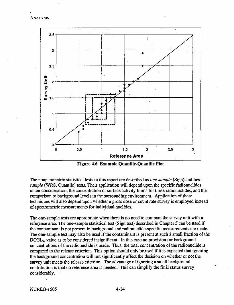
ANALYSIS
I16 ........... •
0*
0 II ** I a
I.I
00.5 1 1.5 2 2.53
Reference Area
Figure 4.6 Example Quantile-Quantile Plot
The nonparametric statistical tests in this report are described as one-sample (Sign) and two-sample (WRS, Quantile) tests. Their application will depend upon the specific fadionuclidesunder consideration, the concentration or surface activity limits for these radionuclides, and thecomparison to background levels in the surrounding environment. Application of thesetechniques will also depend upon whether a gross dose or count rate survey is employed insteadof spectrometric measurements for individual nuclides.
The one-sample tests are appropriate when there is no need to compare the survey unit with areference area. The one-sample statistical test (Sign test) described in Chapter 5 can be used ifthe contaminant is not present in background and radionuclide-specific measurements are made.The one-sample test may also be used if the contaminant is present at such a small fraction of theDCGLw value as to be considered insignificant. In this case no provision for backgroundconcentrations of the radionuclide is made. Thus, the total concentration of the radionuclide iscompared to the release criterion. This option should only be.used if it is expected that ignoringthe background concentration will not sighificantly affect the decision on whether or not thesurvey unit meets the release criterion. The advantage of ignoring a small backgroundcontribution is that no reference area is needed. This can simplify the finhl status surveyconsiderably.
NUREG-1505 4-14

ANALYSIS
The two-sample WRS test (discussed in Chapter 6) should be used when the radionuclide ofconcern appears in background or if measurements are used that are not radionuclide specific.
The two-sample Quantile test discussed in Chapter 7 is used only when the null hypothesis ofScenario B is chosen.
The statistical tests recommended in this report are listed in Table 4.4. In every case, these testsare supplemented by the elevated measurements comparison (cf. Sections 2.6, 3.7.2, 3.8.2 andChapter 8). Other statistical tests may be used provided that the data are consistent with theassumptions underlying their use, as discussed in the next section. The nonparametric testsgenerally involve fewer assumptions than their parametric equivalents. For example, theStudent's t test may be used if the data distribution is consistent with the assumption ofnormality.. If the data do not exhibit a normal distribution, the nonparametric tests will generallyproduce smaller decision error rates.
Table 4.4 Recommended Statistical Tests
Scenario Reference Area Test
A Yes Wilcoxon Rank Sum
A No Sign
B Yes Wilcoxon Rank Sum, Quantile
B No Sign
4.4 Verify the Assumptions of the Statistical Test
An evaluation should be made to determine that the data are consistent with the underlyingassumptions of the statistical testing procedures used. Certain departures from theseassumptions may be acceptable when given the actual data and other information about the study.Much of the information gained in the preliminary data review (Section 4.2) is directly applicableto verifying the assumptions of the statistical tests, and is a major reason for emphasizing their,use.
A statistical test is called robust if it relatively insensitive to departures from its underlyingassumptions. The nonparametric procedures described in this report were chosen because theyare robust for the problem of testing the value of mean concentrations of residual radioactivity ina survey unit. In cases where the data distributions are extremely skewed, these tests may notdetect limited areas with concentration much higher than the, average in the survey unit. This isone reason for supplementing these tests with the elevated measurement comparison.
The nonparametric tests of Chapters 5, 6 and 7 assume that the data from the reference area orsurvey unit consist of independent samples from each distribution. The WRS test assumes thatthe reference area and survey unit data distributions are the same except for a possible shift in themean.
4-15 NUREG-1505
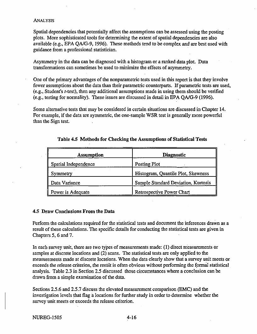
ANALYSIS
Spatial dependencies that potentially affect the assumptions can be assessed using the postingplots. More sophisticated tools for determining the extent of spatial dependencies are alsoavailable (e.g., EPA QA/G-9, 1996). These methods tend to be complex and are best used withguidance from a professional statistician.
Asymmetry in the data can be diagnosed with a histogram or a ranked data plot. Datatransformations can sometimes be used to minimize the effects of asymmetry.
One of the primary advantages of the nonparametric tests used in this report is that they involvefewer assumptions about the data than their parametric counterparts. If parametric tests are used,(e.g., Student's t-test), then any additional assumptions made in using them should be verified(e.g., testing for normality). These issues are discussed in detail in EPA QA/G-9 (1996).
Some alternative tests that may be considered in certain situations are discussed in Chapter 14.For example, if the data are symmetric, the one-sample WSR test is generally more powerfulthan the Sign test.
Table 4.5 Methods for Checking the Assumptions of Statistical Tests
Assumption Diagnostic
Spatial Independence Posting Plot
Symmetry Histogram, Quantile Plot, Skewness
Data Variance Sample Standard Deviation, Kurtosis
Power is Adequate Retrospective Power Chart
4.5 Draw Conclusions From the Data
Perform the calculations required for the statistical tests and document the inferences drawn as aresult of these calculations. The specific details for conducting the statistical tests are given inChapters 5, 6 and 7.
In each survey unit, there are two types of measurements made: (1)'direct measurements orsamples at discrete locations and (2) scans. The statistical tests are only applied to themeasurements made at discrete locations. When the data clearly show that a survey unit meets orexceeds the release criterion, the result is often obvious without performing the formal statisticalanalysis. Table 2.3 in Section 2.5 discussed those circumstances where a conclusion can bedrawn from a simple examination of the data.
Sections 2.5.6 and 2.5.7 discuss the elevated measurement comparison (EMC) and theinvestigation levels that flag a locations for further study in order to determine whether thesurvey unit meets or exceeds the release criterion.
NUREG-1505 4-16
ANALYSIS
This report has been fairly explicit about the steps that should be talken to show that a survey unitmeets release criteria. Less has been said about the procedures that should be used if at any pointthe survey,,unit fails. This is primarily because there are many different ways that a survey unitmay fail the final status survey. The overall level of residual radioactivity may not pass thenonparametric statistical tests. Further investigation following the elevated measurementcomparison may show that there is a large enough area with a concentration too high to meet thedose criterion. Investigation levels may have been flagged during scanning that indicateunexpected levels of residual radioactivity for the survey unit classification. It is impossible toenumerate all of the possible reasons for failure, their causes, and their remedies.
When a survey unit fails the release criterion, the first step is to review and confirm the data thatled to the decision. Once this is done, the extent of the residual radioactivity is that caused thefailure should be determined. Once the cause of failure has been remediated, determine theadditional data, if any, needed to document that the survey unit meets the release criterion.
For example, a Class 2 survey unit passes the nonparametric statistical tests, but has severalmeasurements on the sampling grid that exceed the DCGLw. This is unexpected in a Class 2 area,and according to Table 2.4, these measurements are flagged for further investigation. Additionalsampling confirms that there are several areas where the concentration exceeds the DCGL w Thisindicates that the survey unit was mis-classified. However, the scanning technique that was usedwas sufficient to detect'residual radioactivity at the DCGLEMC calculated for the sample grid. Noareas exceeding the DCGL'EMC where found. Thus, the only difference between the final statussurvey actually done, and that which would be required for Class 1, is that the scanning may nothave covered 100% of the survey unit area. In this case, it would be reasonable to simply increasethe scan coverage to 100%. If no areas exceeding the DCGLEMc are found, the survey unit has, ineffect, met the release criteria as a Class 1 survey'unit.
A second example might be a Class 1 Survey unit which passes the nonparametric statisticaltests, but which contains some ar'eas that were flagged for investigation during scanning. Furtherinvestigation, sampling and analysis indicates one area is truly elevated. This area has aconcentration that exceeds the DCGLw by a factor greater than the area factor calculated for itsactual size. This area is remediated, and remediation control sampling shows that the residualradioactivity was removed, and no other areas were contaminated with removed material. It maybe reasonable in that case, to simply document the original survey and the additional remediationdata. It is not clear that further final status survey data would provide any useful information.
As a last example, consider a Class 1 area which fails the nonparametric statistical tests.Confirmatory data indicates that the average concentration in the survey unit does exceed theDCGLw substantially over a majority of its area. There would appear to be little alternative toremediation of the entire survey unit, followed by another final status survey.
These examples are meant to illustrative of the actions that may be necessary to secure therelease of a survey unit that has initially failed to meet the release criterion. The DQO processshould be revisited so that a plan can be made for attaining the original objective: to safelyrelease the survey unit by showing that it meets the release criteria. Whatever data is necessary tomeet this objective will be in addition to the final status survey data already in hand. All of thedata, and only the data, necessary to meet the objective should be required.
4-17 NUREG-1505


5 SIGN TEST: CONTAMINANT NOT PRESENT IN BACKGROUND
The statistical test discussed in this section is used to compare each survey unit directly with theapplicable release criterion. With only the set of survey unit measurements being analyzed, theSign test used here is called a one-sample test. This section applies if
(1) radionuclide-specific measurements are made to determine the concentrations, and
(2) the background concentration of the radionuclide is negligible.
Otherwise, the methods of Chapter 6 and 7 should be used. Together the above conditionseliminate the need for a reference. The residual radioactivity concentrations in the survey unit arecompared directly to the DCGLw value. The background concentration of the radionuclide neednot be zero, but this background amount will be included with the residual radioactivity whenanalyzing the survey results. The amount that is considered negligible depends on the fraction ofthe DCGLw that it represents, and how much residual radioactivity is actually in the survey unit.The risk of the survey unit failing because the background concentration of the radionuclide isincluded with the residual radioactivity total should be weighed against the savings obtained bynot having to make reference area measurements. Sites need not be contiguous areas, howeverthe statistical test are generally applied to individual survey units that cover contiguous areas.
The Sign test is designed to detect uniform failure of remedial action throughout the survey unit.This test does not assume that the data follow any particular distribution, such as normal orlog-normal. In addition to the Sign Test, the DCGLEMC for the Elevated MeasurementComparison (EMC)-described in Chapter 8-is compared to each measurement to ensure noneexceeds the DCGLEMC. If a measurement exceeds this DCGLEMC, then additional investigation isrecommended-at least locally-to determine the actual areal extent of the elevatedconcentration.
5.1 Introduction
The use of the Sign test in Scenario A and Scenario B is described in the next two sections,illustrated with example data. The same data will be used in both cases. We consider a surveyunit that has been remediated, but may have some residual radioactivity. The DCGLwfor theradionuclide in question has been determined to be 15.9. (The particular radionuclide and units ofmeasurement are irrelevant to the example, and will be left arbitrary.) From data collected duringthe remediation, it is estimated that the standard deviation of the measurements in the survey unitmade during the final status survey should be about 3.3.
During the DQO process it was agreed that the decision error rates should be both set equal to0.05 initially, and determine if a reasonable survey design cduld meet these. It was estimated thatthe costs of additional remediation would be moderate down to concentrations of about 11.5, butwould rise sharply below that. On the basis of these considerations, a chart of the desiredprobability that the survey unit passes was developed and is shown in Figure 5.1.
5-1 NUREG-1505

SIGN TEST
The lower bound of the gray region is 11.5, and the DCGLw is 15.9, so A = 15.9-11.5 = 4.4.Since a is estimated at 3.3, A/( = 4.4/3.3 = 1.3. From Table 3.2, for a = f3 = 0.05, 21 samples arerequired.
100U,a'In' 80
6.
C
S60
= 40
20
1.0I I I
8 10 12 14 16 18 20True Concentration in Survey Unit
Figure 5.1 Desired Probability That.the Survey Unit Passes
The data were taken on a triangular grid. The posting plot is shown in Figure 5.2. It is clear fromthis plot that there is residual radioactivity that is higher near the center of the survey unit andthat diminishes as the survey unit boundary is approached. It is near zero on the west side.
80 N70 N60 N50 N40 N30 N20 N1ONON
-1.1
0.4
0.2
2.0
4.7
16.2119.512.9
23.2
15.5
21.4
26.3
23.6
14.9
17.428.7
10.4
28.410.8
18.5
30 E 40 E
5.8
OE 1OE 20 E
Figure 5.2 Posting Plot of Survey Unit Data
NUREG-1505 5-2

SIGN TEST
The one reported negative value stands out. Negative values can occur whenever an instrument,analysis or blank background is subtracted to obtain a net reading for a sample ', which is thenconverted to a concentration.
Summary statistics for these data are shown in Table 5.1.
Table 5.1 Summary Statistics for Example Data of Figure 5.2
Mean 14.3
Standard Error 2.07
Median 15.5Standard Deviation 9.5
Sample Variance 90.0
Kurtosis -1.09Skewness -0.18
Range 29.8Minimum -1.1Maximum 28.7Count 21
The mean is 14.3, which in this case is actually less than the median, 15.5. This is the influenceof the few low values on the west part of the survey unit, and is also the cause for the slightnegative skewness. The range, 29.8, is only about three times the standard deviation, 9.5. Thisstandard deviation, however, is three times larger than the value of 3.3 assumed in the surveydesign. If the null hypothesis is accepted, the effect of this higher standard deviation on thepower of the test should be investigated. Recall that lower power in Scenario A means that moresurvey units with concentrations that are actually lower than the DCGLw are apt to fail the test.In Scenario B, lower power means that more survey units with concentrations greater than theDCGLw are apt to pass the test. A retrospective power curve, calculated as described in Chapter10, can be used to decide if the error rates achieved are acceptable. A retrospective poweranalysis is not necessary when the null hypothesis is rejected, since the Type I error rate, ax, isfixed at the design value when the critical value for the test is detehnined. However, takingadditional samples to increase the power will increase the Type I error rate, unless provision for atwo-stage test is made during the survey design. This is discussed further in Section 14.2.
A histogram of the data is shown in Figure 5.3. Except for the one negative value in the "zero"bin, the distribution appears reasonably symmetric.
(I For samples with no residual radioactivity, negative values should occur about 50% of the time. It doesnot imply the existence of negative concentrations. Due to random fluctuations, the measurement merely happenedto be lower during the sample analysis than it was during the background determination.
5-3 NUREG-1505

SIGN TEST
1098
7
6543
210
.4
l0ll I400 10 20 30
Figure 5.3 Histogram of Survey Unit Data
Further insight into the distribution of the data can be obtained using a ranked data plot. Table5.2 shows the survey unit data ranked in increasing order. From this table it is already apparentthat there is a large gap between the 6th and 7th ranked values. This is even clearer in the rankeddata plot of Figure 5.4. It seems that there is a mixture of two distributions' in the survey unitdata. One is a distribution of low values near the western edge of the survey unit, and one ofhigher values in the rest of the survey unit. This partially explains the negative skewness and thelarge standard deviation.
Table 5.2 Ranked Data for Example of Figure 5.2
Rank 1 2 3 4 5 6 7
Measurement -1.1 0.2 0.4 2 4.7 5.8 10.4
Rank 8 9 10 11 12 13 14
Measurement 10.8 12.9 14.9 15.5 16.2 17.4 18.5
Rank 15 16 17 18 19 20 21
Measurement 19.5 21.4 23.2 23.6 26.3 28.4 28.7
NUREG-1505 5-4

SIGN TEST
30
25
.o 20
C)
0
-50 5 10
Rank15 20
Figure 5.4 Ranked Data Plot of Survey Unit Data
5.2 Applying the Sign Test: Scenario A
The hypothesis tested by the Sign test under Scenario A is:
Null Hypothesis:
H0: The median concentration of residual radioactivity in the survey unit is greater than the
DCGLw.
versus
Alternative Hypothesis:
H.: The median concentration of residual radioactivity in the survey unit is less than the LBGR.
In order to use the one-sample Sign test, background concentrations of the radionuclide ofconcern are considered to be either zero or insignificant in comparison to the DCGLw Thus,there is no reference to background in statement of the null and alternative hypothesis. The nullhypothesis is assumed to be true unless the statistical test indicates that it should be rejected infavor of the alternative. The parameter of interest is the mean concentration. The median is equalto the mean when the measurement distribution is symmetric, and is an approximation otherwise.
575 NUREG-1505

SIGN TEST
The null hypothesis states that the probability of a measurement less than the DCGLwis less thanone-half, i.e., the 50th percentile (or median) is greater than the DCGL, The median is theconcentration that would be exceeded by 50% of the measurements. Note that some individualsurvey unit measurements may exceed the DCGLw even when the survey unit as a whole meetsthe release criterion. In fact, a survey unit that averages close to the DCGLwmight have almosthalf of its individual measurements greater than the DCGLw. Such a survey unit may still meetthe release criterion.
The hypothesis specifies a release criterion in terms of a DCGLw which is calculated as describedin Section 3.3. The test should have sufficient power (1- 3, as specified in the DQOs) to detectresidual radioactivity concentrations at the Lower Boundary of the Gray Region (LBGR). If a isthe standard deviation of the measurements in the survey unit, then A/a expresses the size of theshift (i.e., A = DCGLw-LBGR) as the nurfiber of standard deviations that would be consideredlarge for the distribution of measurements in the survey unit. The procedure for determining A/awas given in Section 3.8.1.
The Sign test is applied as follows in Scenario A:
(1) List the survey unit measurements, XA,,i = 1, 2, 3..., N. If a measurement is listed as "lessthan" a given value, insert that value for the measurement.
(2) Subtract each measurement, X,, from the DCGLw to obtain the differences:Di =DCGLw - Xi, i = 1, 2, 3..., N.
(3) If any difference is exactly zero, discard it from the analysis, and reduce the sample size, N,by the number of such zero measurements.
(4) Count the number of positive differences. The result is the test statistic S+. N6te that apositive difference corresponds to a measurement below the DCGLw and contributesevidence that the survey unit meets the release criterion.
(5) Large values of S+ indicate that the null hypothesis is false. The value of S+ is compared tothe table of critical values in Section A.3. If S+ is greater than the critical value, k, in thattable, the null hypothesis is rejected.
For the example survey unit data, the calculations are shown in Table 5.3. Notice that when thedata are ranked, it is really only necessary to observe the rank of the smallest measurement belowthe DCGLw in order to determine S+. However, the differences D, = DCGL, - Xi= 15.9 - Xi arealso shown. The number of positive differences, S+ = 11. The critical value of S+ for the SignTest with a = 0.05 and N= 21 is 14. Since S+ is less than 14, the null hypothesis cannot berejected. The survey unit has failed the test.
NUREG-1505 5-6

SIGN TEST
Table 5.3 Calculations for Sign Test in Scenario A
Rank 7IMeasurement: DCGLw - Measurement J Sign
1 -1.1 14.8 +2 .0.2 15.7 +
3 0.4 15.5 +
4 2.0 13.9 +5 . 4.7 .. 11.2 +
6 " 5.8 10.1 +
7 10.4 5.5 +
8 10.8 5.1 +
9 12.9 3.0 +
10 14.9 1.0 +11 15.5 0.4 +
12 16.2 -0.313 17.4 -1.5
14 18.5 -2.6
15 19.5 -3.6
16 .21.4 -5.5 -
17 23.2 -7.3 -
18 23.6 -7.7.19 26.3 -10.4
20 28.4 -12.5 -
21,.: 28.7 . -12.8 ._ - _
5.3 Applying the Sign Test: Scenario B -0
The hypothesis tested by the Sign test under Scenario B is:
Null Hypothesis:
H.: The median concentration of residual radioactivity in the'survey unit is less than the LBGR.
versus
Alternative Hypothesis:
Ha:The median concentration of residual radioactivity in the survey unit is greater than theDCGLw.
In order to use the one-sample Sign test, background concentrations of the radionuclide of
concern are considered to be either zero or insignificant in comparison to the LBGR. Thus,
5-7 NUREG-1505
SIGN TEST
there is no reference to background in statement of the null and alternative hypothesis. The nullhypothesis is assumed to be true unless the statistical test indicates that it should be rejected infavor of the alternative. The Type I error rate, a, is the probability that a survey unit with residualradioactivity at the LBGR will fail to be released. The power, 1 - P3, is the probability that a surveyunit with residual radioactivity at the DCGLw will fail to be released. The parameter of interest isthe mean concentration. The median is equal to the mean when the measurement distribution issymmetric, and is an approximation otherwise.
The Sign test is carried out for Scenario B in a manner very similar to that for Scenario A:
(1) List the survey unit measurements, X,, i = 1, 2, 3..., N. If a measurement is listed as "lessthan" a given value, insert that value for the measurement.
(2) Subtract the LBGR from each measurement, X,, to obtain the differences:Di = Xi - LBGR, i = 1, 2, 3....,N.
(3) If any difference is exactly zero, discard it from the analysis, and reduce the sample size, N,by the number of such zero measurements.
(4) Count the number of positive differences. The result is the test statistic S+. A positivedifference corresponds to a measurement above the LBGR and is evidence that the medianconcentration of residual radioactivity survey unit may exceed it.
(5) Large values of S+ indicate that the null hypothesis is false. The value of S+ is compared tothe table of critical values in Section A.3. If S+ is greater than the critical value, k, in thattable, the null hypothesis is rejected.
For the example survey unit data, the calculations are shown in Table 5.4. Notice that when thedata are ranked, it is really only necessary to observe the rank of the smallest measurement belowthe LBGR in order to determine S- = N - S+. However, the differences D, = X1 - LBGR =Xi - 11.5 are also shown. The number of positive differences, S+ = 13. The critical value of S+for the Sign Test with a = 0.05 and N = 21 is 14. Since S+ is less than 14, the null hypothesiscannot be rejected. The survey unit has passed the test. However, it remains to determine thepower of the test. Since the observed standard deviation is much greater than that estimated forthe test design, it is likely that this survey unit passed simply because there was insufficientpower to detect residual radioactivity at the DCGLw. The power calculation for this example isgiven in Section 10.1.
5.4 Interpretation of Test Results
Once the results of the statistical tests are obtained, the specific steps required to achieve siterelease will depend on the procedures described in the regulatory guide. The following aresuggested considerations for the interpretation of the test results with respect to the release limitestablished for the site.
NUREG-1505 5-8
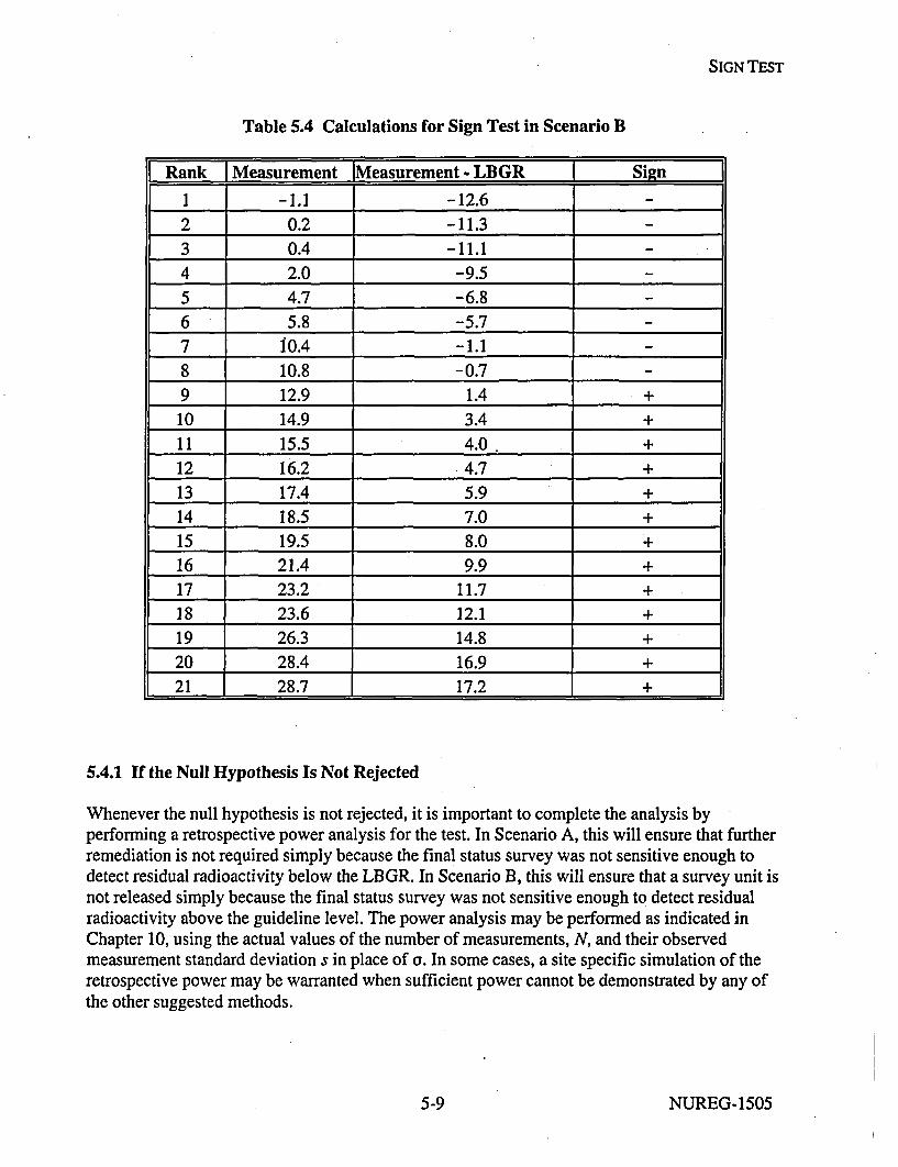
SIGN TEST
Table 5.4 Calculations for Sign Test in Scenario B
Rank T Measurement Measurement - LBGR Sign
1 -1.1 -12.6 -2 0.2 -11.3 -3 0.4 -11.1 -
4 2.0 -9.5 -5 4.7 -6.8 -6 5.8 -5.7 -7 i0.4 -1.18 10.8 -0.79 12.9 1.4 +
10 14.9 3.4 +11 15.5 4.0. +12 16.2 4.7 +13 17.4 5.9 +14 18.5 7.0 +15 19.5 8.0 +16 21.4 9.9 +17 23.2 11.7 +18 23.6 12.1 +19 26.3 14.8 +20 28.4 16.9 +21 28.7 17.2 +
5.4.1 If the Null Hypothesis Is Not Rejected
Whenever the null hypothesis is not rejected, it is important to complete the analysis byperforming a retrospective power analysis for the test. In Scenario A, this will ensure that furtherremediation is not required simply because the final status survey was not sensitive enough todetect residual radioactivity below the LBGR. In Scenario B, this will ensure that a survey unit isnot released simply because the final status survey was not sensitive enough to detect residualradioactivity above the guideline level. The power analysis may be performed as indicated inChapter 10, using the actual values of the number of measurements, N, and their observedmeasurement standard deviation s in place of a. In some cases, a site specific simulation of theretrospective power may be warranted when sufficient power cannot be demonstrated by any ofthe other suggested methods.
5-9 NUREG-1505
SIGN TEST
5.4.2 If the Null Hypothesis Is Rejected
If the null hypothesis for the Sign test is rejected in Scenario A, it indicates that the residualradioactivity in the survey unit is less than the DCGLw. However, it may still be necessary todocument the concentration of residual radioactivity. It is generally best to use the averagemeasured concentration for this purpose.
If the null hypothesis is rejected in Scenario B it indicates that the residual radioactivity in thesurvey unit exceeds the LBGR. In this case it is important to determine not only the averageconcentration of residual radioactivity in the survey unit, 8, but also whether this amount exceedsthe release criteria. When the data are normally distributed, the average concentration is generallythe best estimator for 8. However, when the data are not normally distributed, other estimatorsare often better for the same reasons that nonparametric tests are often better than thecorresponding parametric tests. These methods are discussed by Lehmann and D'Abrera (1975).When the estimate for 6 is below DCGLw, the survey unit may be judged sufficientlyremediated, shbject to ALARA consideiations. Otherwise, further remediation will generally berequired.
The treatment of data that are below the limit of detection will be an important component ofthese calculations. Whenever possible, the actual results of the measurement should be reported,with an associated total uncertainty that includes both random and systematic errors. Replacingvalues below the MDC with the MDC value will cause 8 to be overestimated.
NUREG-1505 5-10

6 WILCOXON RANK SUM TEST:CONTAMINANT PRESENT IN BACKGROUND
The statistical tests discussed in this section will be used to compare each survey unit with anappropriately chosen, site-specific reference area. Each reference area should be chosen on thebasis of its similarity to the survey unit, as discussed in Section 2.2.7.
In Scenario A, the comparison of measurements from the reference area and survey unit is madeusing the Wilcoxon Rank Sum (WRS) test (also called the Mann-Whitney test).
Under Scenario B, the comparison of measurements in the reference area and survey unit is madeusing two nonparametric statistical tests: the WRS test and the Quantile test. The WRS andQuantile tests are both used because each test detects different residual contamination patterns inthe survey units. Because two tests are used, the Type I error rate, ca, specified during the DQOprocess is halved for the individual tests. The Quantile test is discussed in Chapter 7.
In addition to the statistical tests, the EMC is performed against each measurement to assure thatit does not exceed a specified investigation level. If any measurement in the remediated surveyunit exceeds the specified investigation level, then additional investigation is recommended, atleast locally, regardless of the outcome of the WRS or Quantile test.
The WRS test is most effective when residual radioactivity is uniformly present throughout asurvey unit. The test is designed to detect whether or not this activity exceeds the DCGLw. Theadvantage of the nonparametric WRS test is that it does not assume that the data are normally orlog-normally distributed. The WRS test also allows for less than detectable measurements ineither the reference area or the survey unit. As a general rule, the WRS test can be used with upto 40% less than detectable measurements in the reference area and the survey unit combined.However, the use of less than values in data reporting is not encouraged. Wherever possible, theactual result of a measurement, together with its uncertainty, should be reported.
6.1 Introduction
The use of the WRS test in Scenario A and Scenario B are described in the next two sections,illustrated with example data. We consider a Class 2 survey consisting of interior drywallsurfaces, that may have some residual radioactivity. The DCGLw for the radionuclide in questionhas been determined to be 160. (The particular radionuclide and units of measurement areirrelevant to the example, and will be left arbitrary.) The background level is about 40. It isestimated that the standard deviation of the measurements in the survey unit and the referencearea is about 6.
Since the DCGLw is so much larger than a, large sample sizes will not be needed even if theacceptable error rates are set to low values. In this circumstance, the rule of thumb that A/ashould lie between one and three can be used to set the Lower Bound of the Gray Region(LBGR). If, for example, A/a = 3, then A = 18, since a is estimated at 6. The Lower Bound of theGray Region is then LBGR = DCGLw - A = 160 - 18 = 142. If the decision error rates are both
6-j NUREG-1505

WRS TEST
set equal to 0.05 initially, then from Table 3.3, for a = P = 0.05 with A/a = 3, ten samples eachare required in the reference area and the survey unit.
Under Scenario B, the Type I error rate is halved, so cw = a/2 = 0.05/2 = 0.025. Then, againfrom Table 3.3, for a = 0.025, P3 = 0.05, and A/a = 3, twelve samples each are required in thereference area and the survey unit. The corresponding chart of the desired probability that thesurvey unit passes is shown in Figure 6.1. Note that, although the probability that a survey unit atthe LBGR passes the WRS test in Scenario B is 97.5%, the overall probability of passing boththe WRS and Quantile tests is approximately 95%.
Since both scenarios are illustrated using the same set of data, the larger sample size will be usedfor both.
100.
06o
'E
S40-
c oU,
100 120 140 160 180 200
True Concentration Above Background In Survey Unit
Figure 6.1 Desired Probability That the Survey Unit Passes
The data were taken on a triangular grid('), and the posting plot is shown in Figure 6.2. For thisexample the concentration of the radionuclide of interest is given in arbitrary units. It is clearfrom this plot that there is residual radioactivity above background in the survey unit.
Summary statistics for these data are shown in Table 6.1. The mean and median are fairly closein both the reference area and the survey unit. The standard deviations of the data are slightlylarger than estimated during the survey design, but the ratio A/a remains above 2, so the impacton the power of the tests should not be severe. The range of the data is between 3 and 4 standard
(I)A random start systematic grid is used in Class 2 and 3 survey units primarily to limit the size of anypotential elevated areas. Since areas of elevated activity are not an issue in the reference areas, the measurementlocations can be either random or on a random start systematic grid.
NUREG-1505 6-2
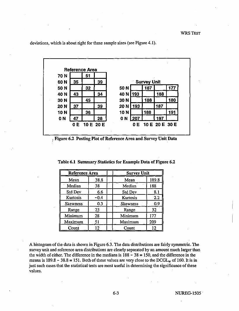
WRS TEST
deviations, which is about right for these sample sizes (see Figure 4.1).
Reference Area70 N 5160 N 35 3950 N 3240 N 43 3430 N 4520 N 37 391ON 360 N M7 28
50 N40 N30 N20 N1ONON
Su -y Unit187 177
193 188
188 180
193 187- 188
- 191
2071 1197 1 1OE 10E 20E 30E
IOE I1E 20E
Figure 6.2 Posting Plot of Reference Area and Survey Unit Data
Table 6.1 Summary Statistics for Example Data of Figure 6.2
Reference Area JJ Survey Unit
Mean 38.8 Mean 189.8Median 38 Median 188Std Dev 6.6 Std Dev 8.1Kurtosis -0.4 Kurtosis 2.2
Skewness 0.3 Skewness 0.9Range 23 Range 32
Minimum 28 Minimum 177Maximum 51 Maximum 209
Count 12 Count 12
A histogram of the data is shown in Figure 6.3. The data distributions are fairly symmetric. Thesurvey unit and reference area distributions are clearly separated by an amount much larger thanthe width of either. The difference in the medians is 188 - 38 = 150, and the difference in themeans is 189.8 - 38.8 = 151. Both of these values are very close to the DCGLW of 160. It is injust such cases that the statistical tests are most useful in determining the significance of thesevalues.
6-3 NUREG-1505

WRS TEST
25 35 45 55 165 175 185 195 205,
Figure 6.3 Histograms of Reference Area and Survey Unit Data
Since there are equal numbers of data in the reference area and in the survey unit, a Quantile-Quantile plot is easily constructed. Table 6.2 shows the reference area and survey unit data eachseparately ranked in increasing order. The pairs of data from the reference area and the surveyunit with the same rank are plotted in Figure 6.4. This is the Quantile-Quantile plot. The positionof the medians is indicated by the solid bar and the central 50% of the data is enclosed in thedashed box. The plot is fairly straight, and the slope is not greatly different from one; indicating:the the shapes of the reference area and survey unit distributions are similar. However, the surveyunit distribution is shifted to values about 150 larger. Again, the significance of this relative tothe DCGLw is precisely what the WRS test is designed to determine.
Table 6.2 Ranked Data for Example of Figure 6.2
Rank jReference Areaj Rank J Survey Unit
1 28 1 1772 32 2 1803 34 3 1874 35 4 1875 36 5 1886 37 6 1887 39 7 1888 39 8 1919 43 9 19310 45 10 19311 47 11 19712 51 1- 212
NUREG-1505 6-4

WRS TEST
210
C 205oE
~200O
g 195
SE 190 ,:• ~~*L ........ ,
>% 185
180
C)
.17525 30 35 40 45 50 55
Reference Area MeasurementFigure 6.4 Quantile-Quantile Plot of Example Data
6.2 Applying the WRS Test: Scenario A
The hypothesis tested by the WRS test under Scenario A is:
Null Hypothesis:
H0: The median concentration in the survey unit exceeds that in the reference area by more than
the DCGLw.
versus
Alternative Hypothesis:
H.: The median concentration in the survey unit exceeds that in the reference area by less than
the LBGR.
The null hypothesis is assumed to be true unless the statistical test indicates that it should berejected in favor of the alternative. One assumes that any difference between the reference areaand survey unit concentration distributions is due to a shift in the survey unit concentrations tohigher values-i.e., due to the presence of residual radioactivity in addition to background. Thesize of this shift is the difference in the mean concentrations. The median is equal to the meanwhen the measurement distributions are symmetric, and is an approximation otherwise.Note that some or all of the survey unit measurements may be larger than some reference areameasurements, while still meeting the release criterion. Indeed, some survey unit measurements
6-5 NUREG-1505

WRS TEST
may exceed some reference area measurements by more than the DCGLW. The result of thehypothesis test determines whether or not the survey unit as a whole is deemed to meet therelease criterion. The EMC is used to screen individual measurements.
Assumptions underlying this test are that (1) the samples from the reference area and the surveyunit are independent random samples, and (2) each measurement is independent of every othermeasurement-regardless of the set of samples from which it came.
The hypothesis specifies a release criterion in terms of a DCGLw which is calculated asdescribed in Section 3.3. The test should have sufficient power (1-3, as specified in the DQOs)to detect residual radioactivity concentrations at the Lower Boundary of the Gray Region(LBGR). If o is the standard deviation of the measurements in the survey unit, then A/0expresses the size of the shift (i.e. A = DCGLw - LBGR) as the number of standard deviationsthat would be considered large for the distribution of measurements in the survey unit. Theprocedure for determining Alo was given in Section 3.8.1.
The WRS test is applied as follows under Scenario A:
(1) Obtain the adjusted reference area measurements, ZI , by adding the DCGLw to eachreference area measurement, Xj. Zi = Xi + DCGLw
(2) The m adjusted reference area sample measurements, Z,, and the n survey unit samplemeasurements, Y,, are pooled and ranked in order of increasing size from I to N, where N =m+n.
(3) If several measurements are tied (have the same value), they are all assigned the average rankof that group of tied measurements.
(4) If there are t less than detectable values, they are all assigned the rank (t + 1)/2. If there ismore than one detection limit, all observations below the largest detection limit should betreated as less than detected. If more than 40% of the data from either the reference area orsurvey unit are less than detectable, the WRS test cannot be used. As stated previously, theuse of less than values in data reporting is not eqcouraged. Wherever possible, the actualresult of a measurement, together with its uncertainty, should be reported.
(5) Sum the ranks of the adjusted measurements from the reference area, W,. Note that since thesum of the first N integers is N(N+1)12, one can equivalently sum the ranks of themeasurements from the survey unit, Ws, and compute W, = N(N + 1)/2 - W,.
(6) Compare W, with the critical value given in Table A.4 for the appropriate values of n, m, anda. If W, is greater than the tabulated value, reject the hypothesis that the survey unit exceedsthe release criterion.
The data for the example are shown in column A of Table 6.3 In column B, the codeR wasinserted to denote a reference area measurement, and S to denote a survey unit measurement. Incolumn A, the data are simply listed as they were obtained. Column C contains the adjusteddata. The adjusted data are obtained by adding the DCGLw to the reference area measurements.
NUREG-1505 6-6

WRS TEST
The ranks of the adjusted data appear in Column D. They range from 1 to 24, since there is atotal of 12 + 12 measurements. The sum of all the ranks is N(N + 1)/2 = (24)(25)/2 = 300.Column E contains only the ranks belonging to the adjusted reference area measurements. Thesum of the ranks of the adjusted reference area data is 199. From Table A.4, for cc = P = 0.05 andn = m = 12, we find that the critical value is 179. Thus, the sum of the reference area ranks, 199,is greater than the critical value, 179, and the null hypothesis that the survey unit concentrationsexceed the DCGLw is rejected. In Scenario A, the survey unit passes.
The analysis for the WRS test is very well suited to the use of a computer spreadsheet. Thespreadsheet formulas in Microsoft ExcelTM (1993) used for the example above are given in Table6.4.
Table 6.3 WRS Test for Class 2 Interior Drywall Survey Unit(Measurements from the reference area and the survey unit are denoted by R and S, respectively)
[ A B C D E1 Data Area Adjusted Data Ranks Reference Area Ranks2 47 R 207 22 223 28 R 188 6.5 6.54 36 R 196 15 155 37 R 197 16.5 16.56 39 R 199 18.5 18.57 45 R 205 21 218 43 R 203 20 209 34 R 194 13 1310 32 R 192 10 1011 35 R 195 14 1412 39 R 199 18.5 18.513 51 R 211 24 2414 209 S 209 23 _
16 197 S 197 16.516 188 S 188 16.5
17 191 S 191 918 193 S 193 11.5 _
19 187 S 187 3.5 _
20 188 S 188 6.5 _
21 180 S 180 2 _
22 193 S 193 11.5 _
23 188 S 188 6.524 187 S 187 3.525 177 S 177 126 Sum= 300 199
6-7 NUREG-1505

WRS TEST
Table 6.4 Spreadsheet Formulas Used in Table 6.3
I A IBI C D E1 Data Area Adjusted Data Ranks Reference Ranks2 47 R =IF(B2="R",A2+160,A2) "RANK(C2,$C$2:$C$25,1) =IF(B2='R",D2,0)
_+(COUNTIF($C$2:$C$25,02) - 1) / 2
3 28 R =IF(B3="R",A3+160,A3) =RANK(C3,$C$2:$C$25,1) =IF(B3="R*,D3,0)I_ +(COUNTIF($C$2:$C$25,C3) - 1) / 2
4 36 R =IF(B4="R*,A4+160,A4) =RANK(C4,$C$2:$C$25,1) =IF(B4="R",D4,0)+(COUNTI F($C$2:$C$25,C4) - 1) / 2
5 37 R =IF(B5="R",A5+160,A5) =RANK(C5,$C$2:$C$25,1) =IF(B5="R",D5,0)+(COUNTIF($C$2:$C$25,C5) - 1) / 2
6 39 R =IF(B6="R",A6+160,A6) =RANK(C6,$C$2:$C$25,1) =IF(B6="R*,D6,0)+(COUNTIF($C$2:$C$25,C6) - 1) / 2
7 45 R =IF(B7=WR',A7+160,A7) =RANK(C7,$C$2:$C$25,1) =IF(B7="R",D7,0)+(COUNTIF($C$2:$C$25,C7) - 1) / 2
8 43 R =IF(B8="R",A8+160,A8) =RANK(C8,$C$2:$C$25,1) =IF(B8="R",D8,O)+(COUNTIF($C$2:$C$25,C8) - 1) / 2
9 34 R =IF(B9="R",A9+160,A9) =RANK(Cg,$C$2:$C$25,1) =IF(B9="R",D9,0)+(COUNTIF($C$2:$C$25,cg) - 1)/2
10 32 R =IF(B10="R*,A10+160,A10) =RANK(C10,$C$2:$C$25,1) =IF(B10="R*,D10,0)+(COUNTIF($C$2:$C$25,C10) - 1)/2
11 35 R =IF(B11="R",A11+160,A11) =RANK(C 1,$C$2:$C$25,1) =IF(B11="R",D11,0)+(COUNTIF($C$2:$C$25,C1 1) - 1) / 2
12 39 R =IF(B1 2="R",A12+160,A12) =RANK(C1 2,$C$2:$C$25,1) =IF(B12="R",D12,0)+(COUNTIF($C$2:$C$25,C12) - 1) / 2
13 '51 R =IF(BI3="R",A13+160,A1 3) =RANK(C1 3,$C$2:$C$25,1) =IF(B13="R",D13,0)+(COUNTIF($C$2:$C$25,C13) - 1) 12
14 209 S =IF(B1 4="R,A1 4+160,A1 4) =RANK(C1 4,$C$2:$C$25,1) =IF(B14=*R",D14,0)+(COUNTIF($C$2:$C$25,C14) - 1) 12
15 197 S =IF(B1 5="R,A1 5+160,A1 5) =RANK(C1 5,$C$2:$C$25,1) =IF(B15="R",D15,0)+(COUNTIF($C$2:$C$25,C15) - 1) / 2
16 188 S =IF(B1 6="R,A1 6+160,A1 6) =RANK(C1 6,$C$2:$C$25,1) =IF(B16=*R",D16,0)+(COUNTIF($C$2:$C$25,C1 6) - 1) / 2
17 191 S =IF(B1 7='R,A1 7+160,A1 7) =RANK(C1 7,$C$2:$C$25,1) =IF(B17="R",D17,0)+(COUNTIF($C$2:$C$25,C17) - 1) / 2
18 193 S =IF(B1 8=R",A1 8+1 60,A1 8) =RANK(CIB,$C$2:$C$25,1) =IF(B18="R",D18,0)+(COUNTIF($C$2:$C$25,018) - 1) / 2
19 187 S =IF(B1 9="R",A1 9+160,A1 9) =RANK(C1 9,$C$2:$C$25,1) =IF(B19="R",D19,0)+(COUNTIF($C$2:$C$25,C19) - 1) / 2
20 188 S =IF(B20="R",A20+160,A20) =RANK(C20,$C$2:$C$25,1) =IF(B20=-"R",D20,0)+(COUNTIF($C$2:$C$25,C20) - 1) / 2
21 180 S =IF(B21="R",A21+160,A21) =RANK(C21,$C$2:$C$25,1) =IF(B21="R",D21,O)+(COUNTIF($C$2:$C$25,C21) - 1) / 2
22 193 S =IF(B22="R",A22+160,A22) =RANK(C22,$C$2:$C$25,1) =IF(B22=*R",D22,0)+(COUNTIF($C$2:$C$25,C22) - 1) / 2
23 188 S =IF(B23="R",A23+160,A23) =RANK(C23,$C$2:$C$25,1) =IF(B23="R",D23,0)+(COUNTIF($C$2:$C$25,C23) - 1) 12
24 187 S =IF(B24="R",A24+160,A24) =RANK(C24,$C$2:$C$25,1) =IF(B24="R",D24,0)+(COUNTIF($C$2:$C$25,C24) - 1) / 2
25 177 S r=IF(B25="R",A25+160,A25) =RANK(C25,$C$2:$C$25,1) =IF(B25="R",D25,0)+(COUNTIF($C$2:$C$25,C25) - 1) /2
26 Sum= 299 =SUM(E2:E25)
NUREG-1505 6-8
WRS TEST
Note that some spreadsheet programs assign the lowest rank in a group of ties to every memberof the group, rather than the average rank for the group. This can be corrected by adding to eachrank the value (g -1)/2, where g is the number of data points in the group. This is the function ofthe COUNTIF statement in column D of Table 6.4.
6.3 Applying the WRS Test: Scenario B
Two tests are used in Scenario B to ensure that there is adequate power to detect a survey unitthat does not meet the release criterion. The concept of the statistical power of a test wasdiscussed in Section 2.3.2. The WRS test has more power than the Quantile test to detectuniform failure of remedial action throughout the survey unit. The Quantile test has more powerthan the WRS test to detect failure of remedial action in only a few areas within the survey unit.These nonparametric tests do not require that the data be normally or log-normally distributed.Measurements reported as non-detects may also be used with these tests, although this practice isdiscouragedt 2). As a general rule, the WRS test can be used with up to 40% less than detectablemeasurements in either the reference area or the survey unit. The Quantile test can be used evenwhen more than 50% of the measurements are below the limit of detection.
In addition, an elevated measurement comparison is conducted. This consists of determining ifany measurements in the remediated survey unit exceed a specified investigation level. If so,then additional investigation is required, at least locally, regardless of the outcome of the WRSand Quantile tests.
The hypothesis tested by the WRS test under Scenario B is:
Null Hypothesis:
HO: The difference in the median concentration of radioactivity in the survey unit and in the
reference area is less than the LBGR.
versus
Alternative Hypothesis:
H.: The difference in the median concentration of radioactivity in the survey unit and in the
reference area is greater than the DCGLw.
The Type I error rate, aw = 02, is the probability that a survey unit with residual radioactivity(above background) at the LBGR will fail this test. The power, 1-3, is the probability that asurvey unit with residual radioactivity at the DCGLw will fail this test.
The WRS test is applied as follows under Scenario B:
(1) Obtain the adjusted survey unit measurements, Z1 , by subtracting the LBGR from each
(2) All actual measurement results (with an associated uncertainty) should be reported, even if they are
negative, so that unbiased estimates of averages can be calculated.
6-9 NUREG-1505

WRS TEST "
survey unit measurement, Y,. Zi = Y1 - LBGR
(2) The n adjusted survey unit measurements, Z , and the m reference area measurements, Xi,are pooled and ranked in order of increasing size from 1 to N, where N = m+n.
(3) If several measurements are tied (have the same value), they are all assigned the average rankof that group of tied measurements.
(4) If there are t less than detectable values, they are all assigned the rank (t + 1)/2. If there ismore than one detection limit, all observations below the largest detection limit should betreated as less than detectable. If more than 40% of the data from either the reference area orsurvey unit are less than detectable, the WRS test cannot be used.
(5) Sum the ranks of the adjusted measurements from the survey unit, W,. Note that since thesum of the first N integers is N(N + 1)/2, one can equivalently sum the ranks of themeasurements from the reference area, W, and compute W, = N(N + 1)/2 - W,.
(6) Compare W, with the critical value given in Table A.4 for the appropriate values of n, m, andaz. If W, is greater than the tabulated value, reject the hypothesis that the difference in themedian concentration between the survey unit and the reference area is less than the LBGR.
The data for the example are shown in column A of Table 6.5 In column B, the code R wasinserted to denote a reference area measurement, and S to denote a survey unit measurement. Incolumn A, the data are simply listed as they were obtained. Column C contains the adjusteddata. The adjusted data are obtained by subtracting the LBGR from the survey unitmeasurements.
The ranks of the adjusted data appear in Column D. They range from 1 to 24, since there is atotal of 12 + 12 measurements. The sum of all the ranks is N(N + 1)/2 = (24)(25)/2 = 300.Column E contains only the ranks belonging to the adjusted survey unit measurements. The sumof the ranks of the adjusted survey unit data is 194.5. From Table A.4, for cew = W2 = 0.025,P = 0.05, and n = m = 12, we find that the critical value is 184. Thus, the sum of the adjustedsurvey unit ranks, 194.5, is greater than the critical value, 184, and the null hypothesis that thesurvey unit concentrations do not exceed LBGR is rejected. In Scenario B, the true survey unitresidual radioactivity is judged to be in excess of 142 above background.
The analysis for the WRS test is very well suited to the use of a computer spreadsheet. Thespreadsheet formulas in Microsoft ExcelTM (1993) used for the example above are given inTable 6.6. Note that some spreadsheet programs assign the lowest rank in a group of ties to everymember of the group, rather than the average rank for the group. This can be corrected by addingto each rank the value (g - 1)/2, where g is the number of data points in the group. This is thefunction of the COUNTIF statement in column D of Table 6.6.
NUREG-1505 6-10

WRS TEST
Table 6.5 WRS Test Under Scenario B for Class 2 Interior Drywall Survey Unit(Measurements from the reference area and the survey unit are denoted by R and S, respectively)
[ A B C D E
1 Data Area Adjusted Data Ranks Survey Unit Ranks
2 47 R 47 18
3 28 R 28 1 _
4 36 R 36 6 _
5 37 R 37 7
6 39 R 39 9.5
7 45 R 45 13
8 43 R 43 11
9 34 R 34 3
10 32 R 32 2
11 35 R 35 4.5
12 39 R 39 9.5
13 51 R 51 21
14 209 S 67 24 24
15 197 S 55 23 23
16 188 S 46 16 16
17 191 S 49 19 19
18 193 S 51 21 21
19 187 S 45 13 13
20 188 S 46 16 16
21 180 S 38 8 8
22 193 S 51 21 21
23 188 S 46 16 16
24 187 S 45 13 13
25 177 S 35 4.5 4.5
26 Sum= 300 194.5
6-11 NUREG-1505

WRS TEST
Table 6.6 Spreadsheet Formulas Used in Table 6.5
LIA BI C D IE_ __ _I1 Data Area Adjusted Data Ranks Survey Unit
Ranks2 47 R =IF(B2='S",A2-142,A2) =RANK(02,$C$2:$C$25,1) =IF(B2="S",D2,0)
+(COUNTI F($C$2:$C$25,C2) - 1) / 2
3 28 R =IF(B3='SA3-142,A3) =RANK(C3,$C$2:$C$25,1) =IF(B3="S",D3,0)_________________+(COUNTIF($C$2:$C$25,C3) - 1) / 2
4 36 R =IF(B4="S",A4-142,A4) =RANK(C4,$C$2:$C$25,1) =IF(B4="S",D4,O)+(COUNTIF($C$2:$C$25,C4) - 1) / 2
5 37 R =IF(B5="S',A5-142,A5) =RANK(C5,$C$2:$C$25,1) =IF(B5="S",D5,0)I +(COUNTIF($C$2:$C$25,C5) - 1) 2
6 39 R =IF(B6="S",A6-142,A6) =RANK(C6,$C$2:$C$25,1) =IF(B6="S",D6,0)+(COUNTIF($C$2:$C$25,C6) - 1)/ 2
7 45 R =IF(B7="S",A7-142,A7) =RANK(C7,$C$2:$C$25,1) =IF(B7="S",D7,O)I +(COUNTIF($C$2:$C$25,C7) - 1) 2
8 43 R =IF(B8="S",A8-142,A8) =RANK(C8,$C$2:$C$25,1) =IF(B8="S",DB,0)÷(COUNTIF($C$2:$C$25,C8) - 1) 2
9 34 R =IF(B9="S",A9-142,A9) =RANK(C9,$C$2:$C$25,1) =IF(B9="S",D9,0).+(COUNTIF($C$2:$C$25,C9) - 1) 2
10 32 R =IF(B1 0="S",A10-142,A10) =RANK(CIO,$C$2:$C$25,1) =IF(B1O="S",D10,0)I_ +(COUNTIF($C$2:$C$25,C10) - 1)/ 2
11 35 R =IF(B11="S",A11-142,A11) =RANK(C 1,$C$2:$C$25,1) =IF(B11 ="S",D11,0)_(COUNTIF($C$2:$C$25,C11) - 1) 2
12 39 R =IF(B12="S",A12-142,A12) =RANK(C12,$C$2:$C$25,1) =IF(B12="S",D12,0)+(COUNTIF($C$2:$C$25,C12) - 1) /2
13 51 R =IF(B13="S",A13-142,A13) =RANK(C13,$C$2:$C$25,1) =IF(B13="S",D13,0)I +(COUNTIF($C$2:$C$25,C13) - 1) / 2
14 209 S =IF(B14="S",A14-142,A14) =RANK(C1 4,$C$2:$C$25,1) =IF(B14="S",D14,0)__________________+(COUNTIF($C$2:$C$25,C1 4) - 1) /2
15 197 S =IF(B1 5="S",A1 5-142,A1 5) =RANK(C1 5,$C$2:$C$25,1) =IF(B15="S",D15,0)+(COUNTIF($C$2:$C$25,Cl 5) - 1) / 2
16 188 S =IF(B16="S",A16-142,A16) =RANK(C1 6,$C$2:$C$25,1) =IF(B1 6="S",D16,0)+(COUNTIF($C$2:$C$25,C16) - 1) / 2
17 191 S =IF(B17="S",A17-142,A17) =RANK(C17,$C$2:$C$25,1) =IF(B17="S",D17,0)+(COUNTIF($C$2:$C$25,C17) - 1) / 2
18 193 S =1F(B18="S",A18-142,A18) =RANK(C18,$C$2:$C$25,1) =IF(B18--"S",D18,0),-+(COUNTIF($C$2:$C$25,C18) - 1) /2
19 187 S =IF(B19="S",A19-142,A19) =RANK(C19,$C$2:$C$25,1) =IF(B19="S",D19,0)+(COUNTIF($C$2:$C$25,C1 9) - 1) / 2
20 188 S =IF(B20="S",A20-142,A20) =RANK(C20,$C$2:$C$25,1) =IF(B20="S",D20,0)I_ +(COUNTIF($C$2:$C$25,C20) - 1) / 2
21 180 S =IF(B21 ="S",A21-142,A21) =RANK(C21,$C$2:$C$25,1) =IF(B21="S",D21,0)I_ +(COUNTIF($C$2:$C$25,C21) - 1) / 2
22 193 S =IF(B22="S",A22-142,A22) =RANK(C22,$C$2:$C$25,1) . =IF(B22="S",D22,0)+(COUNTIF($C$2:$C$25,C22) - 1) / 2
23 188 S =IF(B23="S",A23-142,A23) =RANK(C23,$C$2:$C$25,1) =IF(B23="S",D23,0)I +(COUNTIF($C$2:$C$25,C23) - 1) / 2 r
24 187 S =IF(B24="S",A24-142,A24) -RANK(C24,$C$2:$C$25,1) =IF(B24="S",D24,0),+(COUNTIF($C$2:$C$25,C24) - 1) / 2. ____________
25 177 S =IF(B25-"S",A25-142,A25) =RANK(C25,$C$2:$C$25,1) =IF(B25="S",D25,0)_+(COUNTI F($C$2:$C$25,C25) - 1) / 2
26 Sum= 299 • SUM(E2:E25)
NUREG-1505 6-12

WRS TEST
6.4 Interpretation of Test Results
Once the results of the statistical tests are obtained, the specific steps required to achieve siterelease will depend on the procedures described in the regulatory guide. The following aresuggested considerations for the interpretation of the test results with respect to the release limitestablished for the site.
6.4.1 If the Null Hypothesis Is Not Rejected
Whenever the null hypothesis is not rejected, it is important to complete the analysis byperforming a retrospective power analysis for the test. In Scenario A, this will ensure that furtherremediation is not required simply because the final status survey was not sensitive enough todetect the difference in mean radioactivity concentration between the survey unit and thereference area when that difference is below the LBGR. In Scenario B, this will ensure that asurvey unit is not released simply because the final status survey was not sensitive enough todetect the difference in mean radioactivity concentration between the survey unit and thereference area when that difference is above the guideline level. The power analysis may beperformed as indicated in Chapter 10, using the actual values of the number of measurements, N,and their observed measurement standard deviation s in place of a. In some cases, a site-specificsimulation of the retrospective power may be warranted when sufficient power cannot bedemonstrated by any of the other suggested methods. .
If the null hypothesis for the WRS test is not rejected in Scenario B, the Quantile test describedin Chapter 7 must also be performed.
6.4.2 If the Null Hypothesis Is Rejected
If the null hypothesis for the Sign test is rejected in Scenario A, it indicates that the residualradioactivity in the survey unit is less than the DCGLw. However, it may still be necessary todocument the concentration of residual radioactivity. It is generally best to use the difference inmean radioactivity concentration between the survey unit and the reference area for this purpose.
If the null hypothesis is rejected in Scenario B, it indicates that the residual radioactivity in thesurvey unit exceeds the LBGR. In this case it is important to determine not only the difference inmean radioactivity concentration between the survey unit and the reference area, 8, but alsowhether this difference exceeds the release criteria. When the data are normally distributed, theaverage concentration is generally the best estimator for 8. However, when the data are notnormally distributed, other estimators are often better for the same reasons that nonparametrictests are often better than the corresponding parametric tests. These methods are discussed byLehmann and D'Abrera (1975). When the estimate for 8 is below DCOLw , the survey unit maybe judged sufficiently remediated, subject to ALARA considerations. Otherwise, furtherremediation will generally be required.
6-13 NUREG-1505


7 QUANTILE TEST
The Quantile test was specifically developed to detect differences between the survey unit andthe reference area that consist of a shift, 8', to higher values in only a fraction, E, 0 < E < 1, of thesurvey unit. It should be noted that, in general, this shift, 8', is not necessarily the same as theshift 8 used for the WRS test. The Quantile test is only used in Scenario B. The Quantile test isperformed after the WRS test, if the null hypothesis for that test has not been rejected. Using theQuantile test in tandem with the WRS test in Scenario B results in higher power to detect surveyunits that have not been adequately remediated than either test has by itself.
7.1 Introduction
The specific hypothesis tested by the Quantile test (see Johnson et al., 1987; EPA 230-R-94-004,1994) is:
Null Hypothesis:H 0: c = 0 or8' 6 LBGRversusAlternative Hypothesis:Ha: E > 0 and 8' > LBGR
Simply put, the null hypothesis is that there is no residual radioactivity above the LBGR in anypart of the survey unit. The Quantile test is better at detecting situations in which only a portion,E, of the survey unit contains excess residual radioactivity. The WRS test is better at detectingsituations in which any excess residual radioactivity is uniform across the entire survey unit.
7.2 Applying the Quantile Test
For the Quantile test, the appropriate page in Table A.7 is selected, according to the value Of ca =xc/2.(') Find the nearest values of n, the number of measurements from the survey unit, and m,
the number of measurements from the reference area, that are tabulated. There are three numbersassociated with each tabulated pair of n and m values, namely r, k, and aQ.
The m measurements from the reference area and the n adjusted measurements from the surveyunit are pooled and ranked in order of increasing size from 1 to N, where N = m + n. This is thesame as steps (1) - (3) in Section 6.3 for the WRS test, and the same rankings can be used. If kor more of the r largest measurements in the combined ranked data set are from the survey unit,the null hypothesis is rejected For a survey unit that has failed the WRS test, it is not usuallynecessary to also perform the Quantile test. It is done here as an illustration of the method.
Table 7.1 reproduces the data in Table 6.5, but with two added columns showing the sorted ranksof the adjusted data, and the locition associated with each rank, i.e., R for reference area and Sfor survey unit.
(1) Recall that since the Quantile test is performed in tandem with the WRS test, a Q= Qaw Ca/ 2, so that thethat the size of the two tests in tandem is approximately a = ao+atw
7-1 NUREG-1505

QUANTILE TEST
Table 7.1 Quantile Test Under Scenario B for Class 2 Interior Drywall Survey Unit(Measurements from the reference area and the survey unit are denoted by R and S, respectively)
A B C D E I F G
Data Area Adjusted Ranks Survey Sorted Location1" Data Unit Ranks Associated
Ranks With SortedRank
2 47 R 47 18 - 1 R
3 28 R 28 1 - 2 R
4 36 R 36 6 - 3 R
5 37 R 37 7 - 4.5 R
6" 39 R 39 9.5 - 4.5 S
7 45 R 45 13 - 6 R
8 43 R 43 11 - 7 R
9 34 R 34 3 - 8 S
10 32 R 32 2 - 9.5 R
11 35 R 35 4.5 - 9.5 R
12 39 R 39 9.5 - 11 R
13 51 R 51 21 - 13 R
14 209 S 67 24 24 13 S
15 197 S 55 23 23 13 S
16 188 S 46 16 16 16 S
17 191 S 49 19 19 16 S
18 193 S 51 21 21 16 S
19 187 S 45 13 13 18 R
20 188 S 46 16 16 19 S
21 180 S 38 8 8 21 R
22 193 S 51 21 21 21 S
23 188 S 46 16 16 21 S
24 187 S 45 13 13 23 S
25 177 S 35 4.5 4.5 24 S
26 Sum = 300 194.5 1 1
On the second page of Table A.7, the closest entry to n = m = 12"is for n = m = 10. The valuesof r = 7, k = 6 and 0•Q = 0.029 are found. Thus, the null hypothesis is rejected if 6 of the 7 lafgestadjusted measurements come from the survey unit. From Table 7.1, we find that only 5 of the 7largest adjusted measurements come from the survey unit.
The Quantile test as applied above yields only an approximate result. The values of n and m that
NUREG-1505 7-2
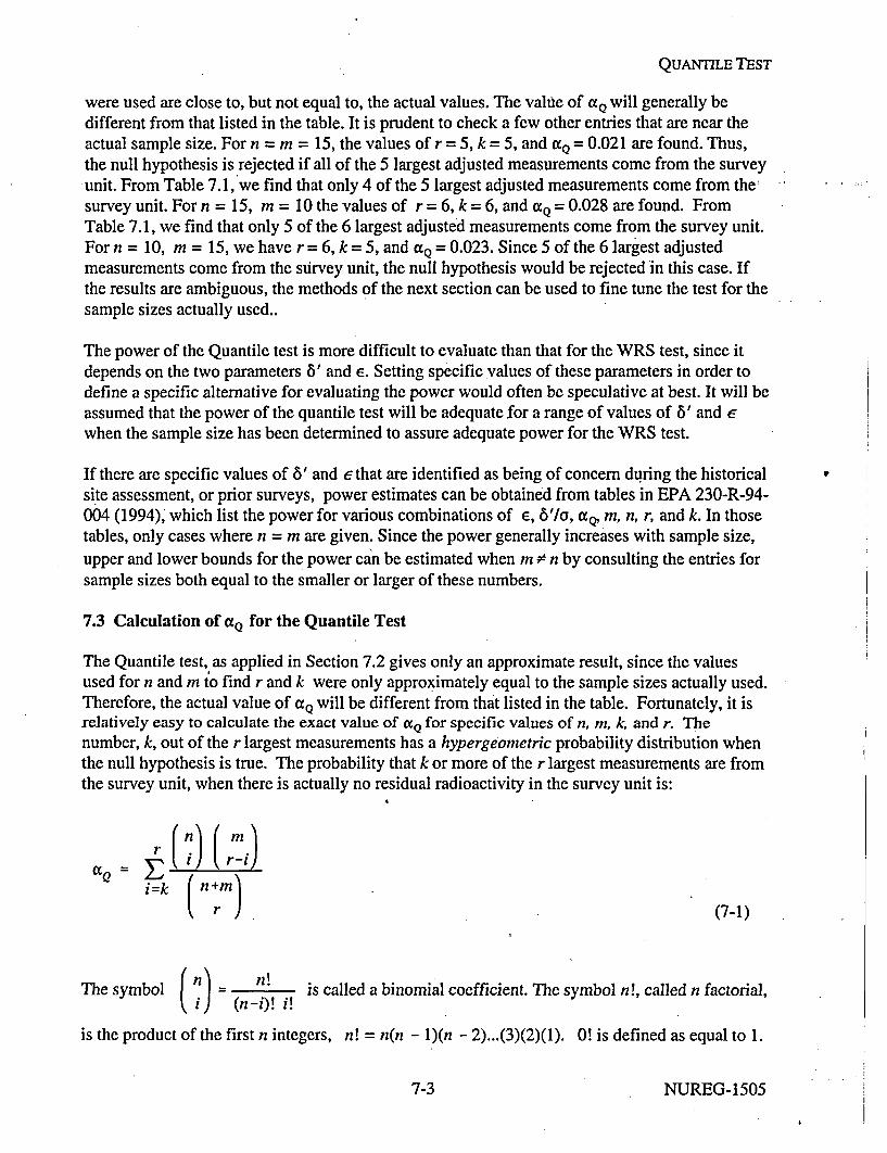
QUANTILE TEST
were used are close to, but not equal to, the actual values. The value of acQ will generally bedifferent from that listed in the table. It is prudent to check a few other entries that are near theactual sample size. For n = m = 15, the values of r = 5, k = 5, and aQ = 0.021 are found. Thus,the null hypothesis is rejected if all of the 5 largest adjusted measurements come from the surveyunit. From Table 7.1, we find that only 4 of the 5 largest adjusted measurements come from the:survey unit. For n = 15, m = 10 the values of r = 6, k = 6, and aQ = 0.028 are found. FromTable 7.1, we find that only 5 of the 6 largest adjusted measurements come from the survey unit.For n = 10, m = 15, we have r = 6, k = 5, and aQ = 0.023. Since 5 of the 6 largest adjustedmeasurements come from the survey unit, the null hypothesis would be rejected in this case. Ifthe results are ambiguous, the methods of the next section can be used to fine tune the test for thesample sizes actually used..
The power of the Quantile test is more difficult to evaluate than that for the WRS test, since itdepends on the two parameters 6' and E. Setting specific values of these parameters in order todefine a specific alternative for evaluating the power would often be speculative at best. It will beassumed that the power of the quantile test will be adequate for a range of values of 6' and ewhen the sample size has been determined to assure adequate power for the WRS test.
If there are specific values of 6' and c that are identified as being of concern during the historicalsite assessment, or prior surveys, power estimates can be obtained from tables in EPA 230-R-94-004 (1994), which list the power for various combinations of E, 6'7o, aQo, m, n, r, and k. In thosetables, only cases where n = m are given. Since the power generally increases with sample size,upper and lower bounds for the power can be estimated when m • n by consulting the entries forsample sizes both equal to the smaller or larger of these numbers.
7.3 Calculation of ccQ for the Quantile Test
The Quantile test, as applied in Section 7.2 gives only an approximate result, since the valuesused for n and m to find r and k were only approximately equal to the sample sizes actually used.Therefore, the actual value of ao will be different from that listed in the table. Fortunately, it isrelatively easy to calculate the exact value of aQ for specific values of n, m, k, and r. Thenumber, k, out of the r largest measurements has a hypergeometric probability distribution whenthe null hypothesis is true. The probability that k or more of the r largest measurements are fromthe survey unit, when there is actually no residual radioactivity in the survey unit is:
Q = E ( r-
i~k ( n+m)i rk (7-1)
The symbol (n! is called a binomial coefficient. The symbol n!, called n factorial,
(d 7) t (n-i) in!
is the product of the first n integers, n! = n(n - 1)(n - 2) ... (3)(2)(1). 0! is defined as equal to 1.
7-3 NUREG-1505
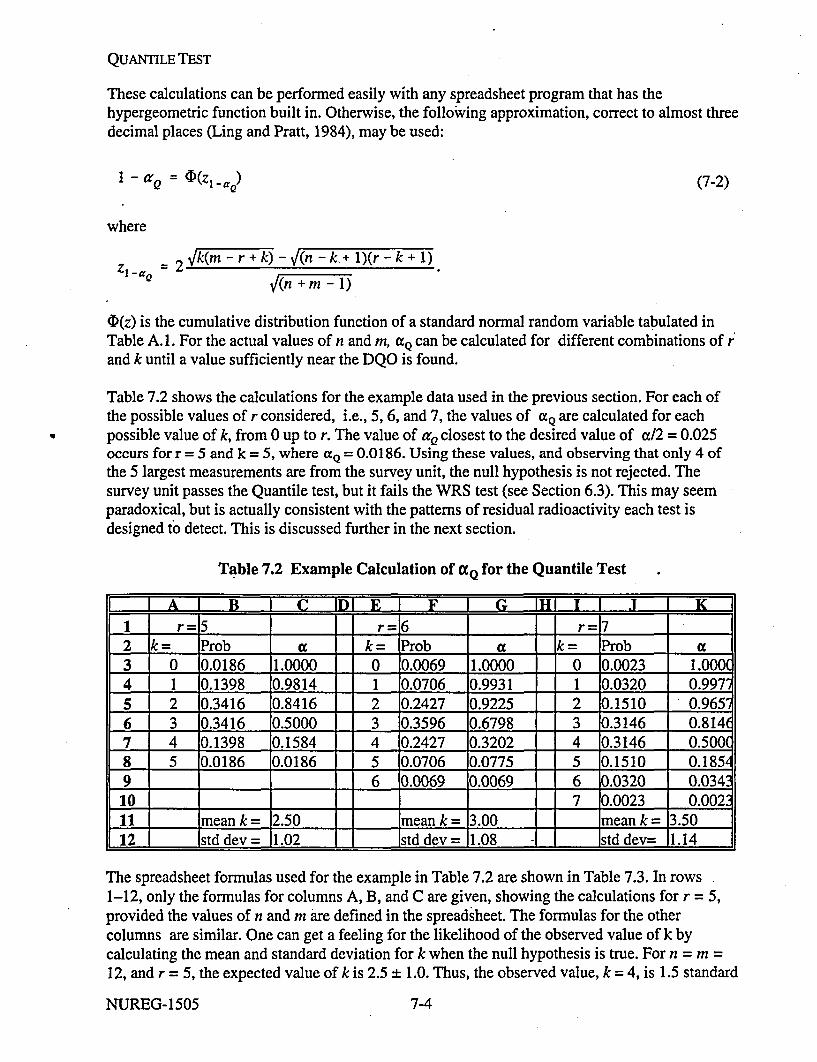
QUANTILE TEST
These calculations can be performed easily with any spreadsheet program that has thehypergeometric function built in. Otherwise, the following approximation, correct to almost threedecimal places (Ling and Pratt, 1984), may be used:
1-'Q =(D(Z1_.) (7-2)
where
= 2 Vk(m - r + -(n - k.+ 1)(r - k + 1)aV(n +m - 1)
4)(z) is the cumulative distribution function of a standard normal random variable tabulated inTable A. 1. For the actual values of n and m, aQ can be calculated for different combinations of rand k until a value sufficiently near the DQO is found.
Table 7.2 shows the calculations for the example data used in the previous section. For each ofthe possible values of r considered, i.e., 5, 6, and 7, the values of aQ are calculated for eachpossible value of k, from 0 up to r. The value of aLQ closest to the desired value of a/2 = 0.025occurs for r = 5 and k = 5, where aQ = 0.0186. Using these values, and observing that only 4 ofthe 5 largest measurements are from the survey unit, the null hypothesis is not rejected. Thesurvey unit passes the Quantile test, but it fails the WRS test (see Section 6.3). This may seemparadoxical, but is actually consistent with the patterns of residual radioactivity each test isdesigned to detect. This is discussed further in the next section.
Table 7.2 Example Calculation of tXQ for the Quantile Test
I A I BZ I C IDI E LL I FL Ju G 111i1iV I I K1 r=5 r=6 r=72 k= Prob a k= Prob a k= Prob a3 0 0.0186 1.0000 0 0.0069 1.0000 0 0.0023 1.000(4 1 0.1398 0.9814 1 0.0706 0.9931 1 0.0320 0.997-5 2 0.3416 0.8416 2 0.2427 0.9225 2 0.1510 0.9656 3 0.3416 0.5000 3 0.3596 0.6798 3 0.3146 0.8147 4 0.1398 0.1584 4 0.2427 0.3202 4 0.3146 0.5008 5 0.0186 0.0186 5 0.0706 0.0775 5 0.1510 0.18599 6 0.0069 0.0069 6 0.0320 0.034
10 7 0.0023 0.00211 mean k = 2.50 meank= 3.00 mean k= 3.5012 std dev = 1.02 std dev = 1.08 1 std dev= 1.14
The spreadsheet formulas used for the example in Table 7.2 are shown in Table 7.3. In rows1-12, only the formulas for columns A, B, and C are given, showing the calculations for r = 5,provided the values of n and m are defined in the spreadsheet. The formulas for the othercolumns are similar. One can get a feeling for the likelihood of the observed value of k bycalculating the mean and standard deviation for k when the null hypothesis is true. For n = m =
12, and r = 5, the expected value of k is 2.5 ± 1.0. Thus, the observed value, k= 4, is 1.5 standard
NUREG-1505 7-4

QUANTILE TEST
deviations above the mean. This is on the high end, but not quite high enough to reject the nullhypothesis.
Table 7.3 Spreadsheet Formulas Used in Table 7.2
A B C1 r= 52 k= Prob a3 0 =HYPGEOMDIST(A3, n, r, n+m) =14 1 =HYPGEOMDIST(A4, n, r, n+m) =1-SUM(B$3:B3)
5 2 =HYPGEOMDIST(A5, n, r, n+m) =1-SUM(B$3:B4)
6 3 =HYPGEOMDIST(A6, n, r, n+m) =1-SUM(B$3:B5)7 4 =HYPGEOMDIST(A7, n, r, n+m) =1-SUM(B$3:B6)
8 5 =HYPGEOMDIST(A8, n, r, n+m) =1-SUM(B$3:7)
91011 mean k= = (n',) I (m+n)
12 std dev = = sqrt( m*n*r'(m+n-1) I (m+n)A2)
7.4 Modified Example for the Quantile Test
It was noted in the previous section that for the example data of Table 7.1 under Scenario B, thesurvey unit would fail the WRS test, yet pass the Quantile test. This occurred because theresidual radioactivity is more or less uniformly distributed across the survey unit. If the exampledata is modified slightly, the result is different. Table 7.4 shows what would happen if 15 units ofresidual radioactivity are subtracted from the first six survey unit measurements and added to thelast six survey unit measurements. The total residual radioactivity measured is unchanged. Theanalysis shows, however, that the sum of the adjusted survey unit measurement ranks is now 178.This is below the critical value of 184 from Section 6.3, and so the survey unit would pass theWRS test. Now, however, all of the highest ranked five measurements are from the survey unit,and so the survey unit would fail the Quantile test. This is because the spatial distribution ofresidual radioactivity is not uniform over the survey unit, but is concentrated at higher values inhalf of the survey unit. The purpose of using the two tests in tandem under Scenario B is todiscover survey units with residual radioactivity in excess of the LBGR. There would be no valuein using two tests if they always gave the same result.
7-5 NUREG-1505
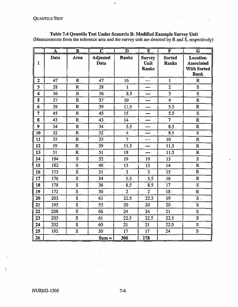
QUANTILE TEST
Table 7.4 Quantile Test Under Scenario B: Modified Example Survey Unit(Measurements from the reference area and the survey unit are denoted by R and S, respectively)
A B C D E F G
Data Area Adjusted Ranks Survey Sorted LocationData Unit Ranks Associated
Ranks With SortedRank
2 47 R 47 16 - 1 R
3 28 R 28 1 - 2 S
4 36 R 36 8.5 - 3 S
5 37 R 37 10 -4 R
6 39 R 39 11.5 - 5.5 R
7 45 R 45 15 - 5.5 S.
8 43 R 43 14 - 7 R
9 34 R 34 5.5 - 8.5 R
10 32 R 32 4 - 8.5 S
11 35 R 35 7 - 10 R
12 39 R 39 11.5 - 11.5 R
13 51 R 51 18 - 11.5 R
14 194 S 52 19 19 13 S
15 182 S 40 13 13 14 R
16 173 S 31 3 3 15 R
17 176 S 34 5.5 5.5 16 R
18 178 S 36 8.5 8.5 17 S
19 172 S 30 2 2 18. R
20 203 S 61 22.5 22.5 19 S
21 195 S 53 20 20 20 S
22 208 S 66 24 24 21 S
23 203 S 61 22.5 22.5 22.5 S
24 202 S 60 21 21 22.5 S
25 192 S 50 17 17 24 S
26 Sum= 300 178 1
NUREG-1505 7-6

8 ELEVATED MEASUREMENT COMPARISON
As discussed in Section 2.6, an Elevated Measurement Comparison is performed by comparingeach measurement from the survey unit to the DCGLEmO If the survey unit is being compared toa reference area, the net survey unit measurement is first obtained by subtracting the mean of thereference area measurements. A net survey unit measurement that equals or exceeds theDCGLEMc is an indication that a survey unit may contain residual radioactivity in excess of therelease criterion.
In addition to direct measurements or samples at discrete locations, parts of each survey unit willalso be scanned. For the quantitative measurements obtained at discrete locations, performing theEMC is a straightforward comparison of two numerical values. Some sophisticated scanninginstrumentation is also capable providing quantitative results with a quality approaching thosefrom direct measurements or samples. Other scanning measurements, however, may be morequalitatiye. In that case, action levels should be established for the scanning procedure so thatareas with concentrations that may exceed the DCGLEMc are marked for a quantitativemeasurement..
8.1 Introduction
The Elevated Measurement Comparison (EMC) against measurements taken on a systematic gridare discussed in Section 8.1. The use of the EMC during scans is discussed in Section 8.2. Areafactors are discussed in Section 8.3, and an example is given in Section 8.4.
The statistical tests may not fail a survey unit when there are only a very few high measurements.The EMC isused so that unusually large measurements will receive proper attention regardlessof the outcome of those tests-and any area that may have the potential for significant dosecontributions will be identified. The EMC is intended to flag potential failures in the remediationprocess, and cannot be used to determine whether or not a site meets the release criterion untilfurther investigation is done.
The derived concentration guideline level for the EMC is: DCGLEMc = (FgS(DCGLw), whereF.d is the area factor for the area of the systematic grid area used (see Section 3.5.4). Note thatDCGLEMc is an a priori limit, established both by the DCGLw and by the survey design (i.e., gridspacing and scanning MDC). The true extent of an area of elevated activity can only bedetermined after performing the survey and then taking additional measurements if an elevatedmeasurement is found. Upon the completion of further investigation, the a posteriori limit,DCGLjy, = (Factuai)(DCGLiy), can be established using the value of the area factor, F, appropriatefor the actual measured area of elevated concentration. The area that is considered elevated isthat bounded by concentration measurements at or below the DCGLw.
If residual radioactivity is found in an isolated area of elevated activity-in addition to residualradioactivity distributed relatively uniformly across the survey unit-the unity rule can be used toensure that the total dose is within the release criterion:
8-1 NUREG-1505
EMC
8 + (average concentration in elevated area - 8) < 1DCGLW (area factor for elevated area)(DCGLw)
If there is more than one elevated area, a separate term should be included for each. As analternative to the unity rule, the dose or risk due to the actual residual radioactivity distributioncan be calculated if there is an appropriate exposure pathway model available.
The preceding discussion primarily concerns Class 1 survey units. Measurements exceedingDCGLw in Class 2 or Class 3 areas may indicate survey unit mis-classification. Scanningcoverage requirements for Class 2 and Class 3 survey units are less stringent than for Class 1survey units.
If the investigation levels of Section 2.6 are exceeded, an investigation should (1) assure that thearea of elevated activity discovered meets the release criterion and (2) provide reasonableassurance that other undiscovered areas of elevated activity do not exist. If further investigationdetermines that the survey unit was misclassified with regard to contamination potential, aresurvey using the method appropriate for the new survey unit classification may be appropriate.
8.2 Comparison Against Individual Measurements
The DCGLmc is calculated on the basis of the grid area, since this is about the same as thelargest circular area that has some chance of being missed when sampling on the grid. Figure 8.1shows both a square and a triangular sampling grid. On the square grid, with grid area L2, thesmall circular area with diameter L has an area of tn(L2)2 = 0.785L2. A circle with area L2 wouldhave a radius of 0.564L. From Figure 3.8, a circle of that radius has only about a 10% chance ofbeing missed. The triangular grid is a little more efficient. The grid area is the rhombus formedfrom two of the triangles, and has area of 0.866L2-. A circle with that area has a radius of0.525L, and, from Figure 3.8, has less than a 5% chance of being missed. The significance of thisis that when no measurement exceeds the DCGLEMo it is unlikely that there are areas remainingthat could cause the release criterion to be exceeded. The survey is planned in anticipation of anegative result, and provides a quantitative measure of risk when no elevated measurements arefound, as well as an objective, dose-based definition of what is considered elevated.
When a measurement is found to exceed the DCGLEMO there is more work to be done before thequestion of compliance can be answered. An individual elevated measurement on a systematicgrid could conceivably represent an area three to four times as large as the systematic grid areaused to define the DCGLEMC. This is the area bounded by the nearest neighbors of the elevatedmeasurement location, as shown by the large circles in Figure 8.1. However, the elevated areamay also be smaller than the grid area. Since the allowable concentration generally increases asthe elevated area decreases in size, further investigation is necessary to determine both the actualarea and average concentration. The boundary of the elevated area is defined by concentrationmeasurements at or below the DCGLW. Once the actual elevated area is found, the correspondingarea factor, Factuai is calculated in order to determine the release criterion for the elevated area:DCGLA = (F,,ctu•)(DCGLw).
NUREG-1505 8-2

EMC
Figure 8.1 Square (top) and Triangular (bottom) Sampling Grids and Grid Areas(Circular elevated areas of radius LJ2 and L are shown for comparison)
The problem remaining is to determine whether or not the average concentration in the elevatedarea meets the DCGLJ.. This is essentially the same problem as the original one of determiningwhether or not the average concentration in the survey unit meets the DCGL, This is not tosuggest that it is necessary to define the elevated area as a separate survey unit and conduct a newsurvey to determine its compliance with the DCGLE. For cases in which the decision is too closeto call, it may be useful to keep this analogy in mind when planning a resolution to the problem.It will also be useful in planning the investigation of the elevated area.
There will be many types and sizes of elevated areas. In many cases, it may be obvious whetheror not the elevated area exceeds the release criterion based on the measurements taken during theinvestigation, without performing an additional survey or performing additional statistical tests.Obviously, -if the elevated area mean exceeds the DCGL A, the survey unit fails. If the elevatedarea mean is less than the DCGLEby more than the standard error of the mean, ALARA
8-3 8-3 NUREG-1505

EMC
considerations will usually determine whether or not further remediation is necessary. As withany measurements, the DQO process should be used in planning the investigation of the elevatedarea, and what decisions will be made based on the results.
Some other considerations that may arise are:
(1) The variability of concentrations in the elevated area is likely to exceed that of anybackground variations, so additional reference area measurements will not usually beneeded. If the survey unit is being compared to a reference area, the boundary of theelevated area should be determined by measurements at or below the DCGL wadded tothe mean reference area measurement. The elevated area mean minus the mean referencearea concentration should not exceed the DCGLEA.
(2) There may be elevated areas within the elevated area: There may exist a smaller areawithin the elevated area that has concentrations high enough to exceed the releasecriterion when considered separately, even though the average concentration over theentire elevated area is within the DCGLEA.
8.3 Comparison Against Scanning Measurements
The measurement results obtained during scanning are inherently more qualitative in nature thanthose obtiined on the systematic grid. In Class 1 survey units, much of the survey design dependson the ability to detect areas exceeding the DCGLESIc during scanning. This is the essence of therequirement that the scanning MDC be below the DCGLEMc. In practice, this means that anoperating procedure for flagging suspect locations during scanning be devised to ensure thatpotential elevated areas be investigated. Then, as is the case with measurements on the systematicgrid that exceed the DCGLEMCo the suspect area must be investigated to determine the area andaverage concentration of the elevated area. In many cases, it would be prudent to set the criteriafor flagging elevated areas conservatively. If this is done, and subsequent quantitativemeasurements indicate that the DCGLEMC is not actually being exceeded, nothing further wouldgenerally be necessary unless for ALARA considerations. If measurements above the statedscanning MDC are found by sampling or by direct measurement at locations that were notflagged by the scanning survey, this may indicate that the scanning method did not meet theDQOs.
Scanning requirements for Class 2 and Class 3 survey units are less stringent both with regard tothe coverage and sensitivity. This is possible because of the screening process necessary to showthat these areas are not highly contaminated (Sections 2.2.2 and 2.2.3). For this reason, theinvestigation levels are lower than in Class 1 areas (Section 2.5.7).
8.4 Area Factors
Area factors have been discussed in Sections 2.2.1 and 3.8.2. These area factors should becalculated using dose pathway models and assumptions that are consistent with those used tocalculate the DCGLw. In this section, examples of area factors for both indoor and outdoorsurvey units are given.
NUREG-1505 8-4

EMC
The example outdoor area factors listed in Table 8.1 were calculated using RESRAD forWindows 5.70 (ANL/EAD/LD-2). For each radionuclide, all dose pathways were calculatedassuming an initial concentration of 1 pCi/g. The default area of contamination in RESRAD 5.7is 10000 m2, so for this size area, the area factor for all radionuclides is equal to one. Areafactors for other size areas were computed by taking the ratio of the dose per unit concentrationcalculated by RESRAD for the default 10000 m2 to that calculated for 1, 3, 10, 30, 100, 300,1000, and 3000 m2. The other RESRAD default values were not changed except to adjust thelength parallel to aquifer to be consistent with area of contamination..
The area factors for selected radionuclides are plotted in Figure 8.2. There it can be seen thatradionuclides generally fall into three groups. Those that deliver dose primarily through internalpathways, those that deliver dose primarily through the external pathway, and a few for whichboth are important. Generally, the radionuclides that deliver dose via internal pathways (e.g.,14C, 9°Sr) have the highest area factors. These area factors scale with the area in a manner
suggesting that it is the total inyentory of the radionuclides that is most important. The areafactors for radionuclides that deliver dose primarily through external gamma have lower areafactors, reflecting the fact that these radionuclides can deliver dose at a distance. In a mixture, itwill generally be these radionuclides that will have the limiting area factors. Fortunately, theseare also the radionuclides most easily detected using scanning techniques.
Notice that Figure 8.2 is plotted on a log-log scale. Linear interpolation on this figurecorresponds to logarithmic interpolation in Table 8.1 for areas between those listed. For example,if the area factor for 24SAm is needed for 25 m2, the table lists 96.3 for 10 m2 and 44.2 for 30 m2.To interpolate, take the base 10 logarithms of these numbers:
loglo (10) = 1loglo (30) = 1.477loglo (25) = 1.398loglo (13.4) =1.127loglo (4.99) = 0.698.
The interpolation is done using these values:
loglo (A25) ' logl0 (13.4)+ [ logl0 (25) - log10 (10)] ([loglo (4.99) - (log1 o (13.4)]i [loglo (30) - loglo (10)])
= 1.127 + [1.398 - 1)] [ 0.698 - 1.127] / [1.477 - 1]
1.127 + [0.398] { [ - 0.429] / [0.477]1
=0.769
Therefore, A2s = 10(0.769) = 5.88.
Example indoor area factors listed in Table 8.2 were calculated using RESRADBUILD forWindows 2.11 (ANL/EAD/LD-3, 1994). For each radionuclide, all dose pathways werecalculated assuming an initial concentration of 1 pCi/m2. The default area of contamination in
8-5 NUREG-1505

EMC
RESRAD BUILD is 36 M 2. The other areas compared to this value were 1, 4, 9, 16, or 25 n2. Noother changes to the RESRAD BUILD default values were made. Dose was computed for onereceptor, who spent 100% of time in the contaminated room. The area factors were thencomputed by taking the ratio of the dose per unit concentration calculated by RESRAD BUILDfor the default 36 M2 to that calculated for the other areas listed. Thus, if the guideline limitconcentration for residual radioactivity distributed over 36 m2 is multiplied by this value, theresulting concentration distributed over the specified smaller area delivers the same averagedose. There are obviously many other exposure scenarios which may result in different areafactors.
Table 8.1 Example Outdoor Area Factors
Nuclide 1000Dm2 3000 m2 1000 m2 300 m2 100 m' 30 m2 10 m2 3 m2 1 m2
Am-241 1.00 1.01 1.01 1.20 1.86 4.99 13.4 40.2 109C-14 1.00 2.09 3.06 4.84 8.40 23.6 65.7 207 609
Cd-109 1.00 1.03 1.04 1.11 1.42 3.05 7.61 22.1 63.0Ce-144 1.00 1.03 1.04 1.11 1.21 1.49 2.05 4.24 9.30Co-57 1.00 1.03 1.05 1.11 1.19 1.46 1.99 4.06 8.69Co-60 1.00 1.04 1.06 1.13 1.23 1.52 2.12 4.39 9.81Cs-134 1.00 1.07 1.10 1.19 1.30 1.61 2.22 4.57 10.1Cs-137 1.00 1.10 1.14 1.28 1.41 1.75 2.41 4.98 11.0Eu-152 1.00 1.03 1.05 -1.10 1.19 1.47 2.03 4.20 9.28Fe-55 1.00 2.12 3.12 9.97 27.1 71.6 149 284 484H-3 1.00 1.06 1.08 1.38 2.18 5.97 16.4 51.3 150
1-129 1.00 1.19 1.34 1.90 3.14 8.92 25.0 79.1 233Mn-54 1.00 1.03 1.05 1.12 1.22 1.50 2.08 4.30 9.52Na-22 1.00 1.05 1.08 1.13 1.22 1.51 2.07 4.28 9.44Nb-94 1.00 1.01 1.05 1.18 1.27 1.56 2.15 4.42 9.77Ni-63 1.00 1.46 1.68 5.59 16.6 54.2 155 464 1180Pu-238 1.00 1.02 1.04 1.82 2.50 3.26 4.24 6.01 8.88Pu-239 1.00 1.02 1.03 1.83 2.51 3.28 4.26 6.07 8.94Ru-106 1.00 1.01 1.02 1.07 1.36 2.65 7.23 14.9 32.7Sb-125 1.00 1.03 1.05 1.10 1.18 1.45 1.99 4.10 8.94Sr-90 1.00 1.17 1.23 4.04 11.9 37.1 98.7 285 729Tc-99 1.00 1.02 1.07 1.54 2.55 7.16 20.0 62.8 185Th-232 1.00 1.03 1.05 1.47 1.75 2.24 3.12 6.08 12.3U-235 1.00 1.01 1.19 2.18 3.84 10.3 15.9 30.2 58.8U-238 1.00 1.01 1.04 1.43 2.27 5.73 11.1 18.3 30.5Zn-65 1.00 1.31 1.45 1.81 2.07 2.62 3.64 7.62 17.0
NUREG-1505 8-6

EMC
Figure 8.2 Example Outdoor Area Factors
The indoor area factors for selected radionuclides are plotted in Figure 8.3. There is not as muchvariation between radionuclides as there is with the outdoor area factors. All of the area factorsscale nearly with the size of the contaminated area. As with the outdoor area factors, theradionuclides that deliver dose primarily through internal pathways have higher area factors thanthose that deliver dose primarily through the external pathway. The area factors for radionuclidesthat deliver dose primarily through internal pathways scale with the area in a manner suggesting
8-7 NUREG-1505

EMC
that it is the total inventory of the removable fraction of these radionuclides that is mostimportant.
Table 8.2 Example Indoor Area Factors
Nuclide 36 m2 25 m2 16 m' 9 m2 4 m2 I m,Co-60 1.0 1.2 1.6 2.5 5.5 22.7Cs-137 1.0 1.2 1.7 2.6 5.7 23.5
H-3 1.0 1.4 2.3 4.0 9.0 36.0Ni-63 1.0 1.4 2.3 4.0 9.0 36.0
Pu-239 1.0 1.4 2.3 4.0 9.0 36.0Ra-226 1.0 1.4 2.1 3.6 8.0 32.2Sr-90 1.0 1.4 2.2 4.0 8.9 35.7
Th-232 1.0 1.4 2.3 4.0 9.0 36.0U-235 1.0 1.4 2.2 4.0 9.0 35.8Zn-65 1.0 1.2 1.6 2.5 5.4 22.3
I-.LL. 10.0
U0m
--- CO-6O
--- "CS-131
:-S-,.'.. H 4 '
•NI-63
• -K-PU-2-31
--- RA.221
-S-- 8R-90
- TH-239
- U-235
- ZN-65
10 100
Area (square meters)
I
Figure 8.3 Example Indoor Area Factors
NUREG-1505 8-8

EMC
The area factors for radionuclides that deliver dose primarily through external gamma have lowerarea factors, reflecting the fact that this dose can be delivered at a distance. Thus, in a mixture, itwill generally be these radionuclides that will usually have the limiting area factors. However,the effect is not as large indoors as outdoors.
8.5 Example
A concrete room, 5 meters by 6 meters, had been contaminated with '37Cs and 6Co, andsubsequently remediated. The floor and the bottom 2 meters of the walls were to be surveyed as aClass 1 survey unit. Measurements were to be made for 100s at each grid point with a 16 cm2
GM counter with a 10.1% efficiency. The DCGLw for both'nuclides were within about 10%, sothe lower was taken to conservatively apply to both. This DCGLw, about 1100 dpm per 100 cm 2,translated into 30 counts per 100s with this detector. During the DQO process it was determinedthat Scenario A would be used with a = 0.05, f3 = 0.025, and A = 10 counts. The averagebackground readings for this type of building on site had been about 60 ± 10 counts, so theestimated a = 10. From Table 3.3, it was found that 39 measurements each were required in thereference area and the survey unit. This was rounded up to 40. The survey unit area is 61 m', sothe spacing, L, on a triangular grid is L = [61/ (0.866N)]' = [61/ (34.6)]" = 1.3 m, usingN= 40. The grid area is 0.866 L2 = 0.866 (1.3)2 = 1.5 m2 . Interpolating into Table 8.2 gives anarea factor for 1.5 m2 of 15. This results in a DCGLEMC = 15 (DCGLw) = 16500 dpm per 100 cm2,.or 450 GM counts per 100s. This level is easily seen while scanning, so no additional gridmeasurements will be needed in order to find elevated areas.
When the random start triangular grid was laid out in the survey unit, 50 measurement locationswere identified. When there are more locations identified than are required, they are all sampledand reported. In the reference area, the grid lay out was terminated when 40 locations werefound. The data are shown in Table 8.3.
The mean and standard deviation of the reference area measurements was 58 ± 10. For the surveyunit, these were 88 ± 92. The difference of the means, 88 - 58, is just at the DCGLw of 30.However the median in the reference area is 59 while that in the survey unit is only 58. This is anindication that the survey unit data is fairly symmetric, but that the survey unit mean is beingdriven up by a few very high measurements. This can be seen even more clearly in the combinedranked data plot of Figure 8.4. For this plot the reference area measurements, adjusted by addingthe DCGLw to each, are combined with the survey unit measurements. The measurements arethen plotted against their rank in the combined data set, using different symbols for the referencearea points and the survey unit points. This is an easier diagnostic plot to.use than the Quantile-Quantile plot when the reference area and survey unit have different numbers of data points.From this plot it can be seen that the majority of the survey unit measurements fall below theadjusted reference area measurements, but that there are eight survey unit measurements that aremuch higher. One of those measurements exceeds the DCGLEMo which is equivalent to 450 GMcounts per 100s. Thus, further investigation of this survey unit will be required before it could bereleased, regardless of the outcome of the WRS test.
The sum of the adjusted reference area ranks, shown in Table 8.3, is 2432. This is greater thanthe critical value of 2023 given by the equation following Table A.3 for n = 50, m = 40, anda = 0.05. Thus, the hypothesis that the survey unit as a whole uniformly exceeds the DCGLw is
8-9 NUREG-1505

EMC
rejected. Whether or not the survey unit may be released is now dependent on the results of theinvestigation of the elevated measurements that were found.
A posting plot of the survey unit data is shown in Figure 8.5. In terms of GM counts, the elevatedarea is defined by the average reference area measurement plus the DCGL w which is58 + 30 = 88. The shaded area in Figure 8.5 encloses the measurements exceeding 88 GM countsper 100s. This area, which also encloses all of the measurements exceeding the DCGL Emo coversalmost 16 m2 . From Table 8.2, the area factor for `aTCs is 1.7 and that for 60Co is 1.6. For amixture of the two radionuclides, the smaller value is used. Thus, in this case the DCGLE = 1.6(DCGLw) = 1760 dpm per 100 cm2, or 48 GM counts per 100s. The average of the tenmeasurements in the shaded area is 216.8 GM counts per 100s, which is 216.8 - 58 = 158.8 GMcounts per 100s above the reference area average. Thus, the survey unit does not meet the releasecriterion, and may not be released without further remediation.
This example illustrates how the nonparametric statistical tests used in combination with theelevated measurement comparison work to assure that the release criterion is met.
500"
450 * Reference Area + DCGL
400 t3Survey Unit
350- t
300
250 0
200
150 0
100" • C 0 r 0a nnt•:]
50 r' 0 0CP 13 0 0 0 13 3r3 0 0 u
0 - 1 I
0 10 20 30 40 50 60 70 80 90
Figure 8.4 Combined Ranked Data Plot of Reference Area and Survey Unit Measurements
NUREG-1505 8-10

EMC
Table 8.3 -Data for Indoor Survey Unit and Reference Area(GM counts per 100s)
Ref Survey Adjusted Ref SurveyData Data Ref Data Ranks Ranks
55 56 88 55 23.550 46 .83 48. 763 55 96 70.5 2251 58 84 52 2743 68 76 -39.5 35.550 51 83 48 .1650 83 83 48 4850 89 83 48 5650 47 83 48 953 134 86 54 8635 410 68 35.5 8950 78 83 48 42.543 52 76 39.5 18.573 40 106 79 2.563 111 96 70.5 8375 340 108 80 8860 50 o93 65 13.558 43 91 59 670 62 103 77.5 30.561 495 94 67.5 9068 63 101 76 3257 47 . 90 57 963 52 96 70.5 18.560 254 93 65 8758 78 91 59 42.559 67 92 62 3347 97 80 44 73.558 59 91 59 2976 49 109 81.5 11.561 118 94 67.5 8470 120 103 77.5 8567 77 100 75 4160 42 93 65 4.576 53 109 81.5 20.552 68 85 53 35.559 68 92 62 35.541 36 74 38 1.63 62 96 70.5 30.564 56 97 73.5 23.559 58 92 62 27
______ 47 _ ____ 940 ______ 2.5
50 _____ 13.5
57 ______ 25
_____ 58 ___________ 27-
49 ___________ 11.5
______ 53 ______ _____ 20.5
_____ .51 ______ .16
42 *4.5
51 16_. _ 243?2 16631
8-11 8-11 NUREG-1505

EMC
Figure 8.5 Posting Plot of Indoor Concrete Survey Unit
NUREG-1505 8-12

9 SAMPLE SIZE
9.1 Sample Size and Decision Errors
To determine the number of samples to collect, acceptable values of the Type I error rate (a) andType H error rate (P3) must be specified as part of a statistical test. The process for doing this wasdiscussed in Section 3.7. If there are many survey units and each unit requires a separatedecision, even if H0 is true approximately 100a% of the times the test is conducted, the nullhypothesis will be incorrectly rejected. If a smaller value of a is used, the number of times thiscan be expected to happen decreases proportionately. On the other hand, larger values of a willreduce the number of samples initially required from each survey unit.
The power (1- 3) is the ability of a statistical test to detect when the null hypothesis is indeedfalse and should be rejected. A test should have high power, i.e., small 13, but smaller specifiedvalues of P3 require a larger number of measurements.
The number of samples depends not only on a and f3, but also on the width of the gray regionrelative to the measurement variability, A/a. This parameter essentially describes the resolutionof the decision problem. When the resolution is high, only a few measurements are needed.When the resolution is low, many more measurements may be required, even though thespecified a and P3 are unchanged.
The DQO steps desciibed in Sections 3.7 and 3.8 are used to balance the cost of sampling againstthe risks involved with any potential decision errors. It is important to realize, however, that thevalue of a is fixed at the desired value when the critical value for the test statistic is determinedfrom the provided tables and used in the test. If the sample size is larger (or smaller) thanplanned, the effect will be an increase (or decrease) in the power, 1- j3. Similarly, if themeasurement standard deviation is larger (or smaller) than anticipated, the effect will be adecrease (or increase) in the power.
The consequences of increasing or decreasing the power depends on whether Scenario A orScenario B is being used. In Scenario A, where the null hypothesis is that the survey unit doesnot meet the release criterion, high power means that a survey unit that meets the release criterionhas a high probability of passing the test. In Scenario B, where the null hypothesis is that thesurvey unit meets the release criterion, high power means that a survey unit that does not meetthe release criterion has a high probability of failing the test.
In most cases, the sample sizes required can be determined using Tables 3.2 and 3.3. In thefollowing sections, the assumptions made and the calculations performed in creating these tablesare described. Methods for modifying the calculations under alternative assumptions are alsogiven. It must be emphasized that relatively little effort is required to perform the suggestedsample size determinations compared to the time and expense involved in collecting andanalyzing samples. This is a key advantage to using the DQO process to determine sample sizes.
9-1 NUREG-1505

SAMPLE SIZE
9.2 Sample Size Calculation for the Sign Test Under Scenario A
For the Sign test, the number of samples, N, required from the survey unit can be approximatedfrom a formula given by Noether (1987):
N - (Z1 -+Z 1 -) 2 (9-1)4 (p -0.5)2
where:a = specified Type I error rate13 = specified Type II error rateZ =. 100(1- a) percentile of the normal distributionZI.p = 100(1- 13) percentile of the normal distributionp = estimated probability that a random measurement from the survey unit will be less than the
DCGLw when the survey unit median is actually at the LBGR. pt 0.5
Commonly used values for a and 13, and the corresponding values of ZI., (or Z,.,) may be foundfrom Table 9.1. Other values can be obtained using any table of the cumulative standard normaldistribution function, such as that in Appendix A.
Table 9.1 Some Values of Z,.. and Z,.p Used To Calculate the Sample Sizes
S(or 13) IZ 1.,, (or Z,-p)0.01 2.3268
0.025 1.9604
0.05 1.6452
0.10 1.2817
0.20 0.8415
The numerator of Equation 9.1, (Z,-,, + Z1 _p )', depends on a and 13, but not on A or a. Inaddition, it only depends on the pair of values used for a and 13, and is the same if these valuesare reversed. This can be seen in the symmetry of Table 9.2, where the value of (Z,-. + Z1 _p )2 isgiven for each pair of the values of a and 13 listed in Table 9.1. As will be seen, these are also theminimum samples sizes for each pair of a and 13 values.
The denominator of Equation 9.1 depends on the parameterp, but not on a or 13. The definition.of the parameter p states that it is the estimated probability that a random measurement from thesurvey unit will be less than the DCGLw when the survey unit median is actually at the LBGR.
This is illustrated in Figure 9.1. The value of I -p expresses the likelihood that measurementsexceeding the DCGLw will be observed, even if half of the concentration distribution is belowthe LBGR. This likelihood is higher when the measurement standard deviation is large compared
NUREG-1505 9-2

SAMPLE SIZE
to the width of the gray region. Some assumptions about the data distribution have to be made inestimating p. If it were possible to specify p exactly, there would be no need to do the survey.
Table 9.2 Some Values of (Z-._ + Zjp )' Used To Calculate Sample Sizes
I 0.01 1 0.025 1 0.05 1 0.1 0.20.01 22 19 16 14 11
0.025 19 16 13 11 8
0.05 16 13 11 9 7
0.1 14 11 9 7 5
0.2 11 8 7 5 3
The relative width of the gray region, A/a, is especially useful for estimating the parameter p. Ifthe data are even approximately normally distributed, then p can be estimated from
DCGL.P I f e -(x-LBGR)
2/2o 2dx
- f e (xLBGRe)2O2 dx
A
f efe-x2/ dx
(9-2)
Values of p as a function of A/c, computed from Equation 9-2, can be found in Table 9.3, or inthe table of the cumulative normal distribution (Appendix A, Table A. 1).
The factor 1/[4(p - 0.5)2 ] in Equation 9-1 can be viewed as a multiplier applied to the samplesizes given in Table 9.2. If p = 1, this factor is one. Figure 9.2 shows the dependence of both pand the sample size multiplier on the resolution of the decision problem, A/a. Increasing A/abeyond about three has little effect on reducing the sample size multiplier. Decreasing A/a belowabout one causes the sample size multiplier to rise dramatically. The range from the smallest (3)to largest (22) sample size in Table 9.2 is about a factor of seven. When A/a is less than about0.5, the sample size multiplier exceeds seven. Thus, small values of A/a can have a bigger impacton increasing the sample size than the choice of acceptable decision error rates.
9-3 NUREG-1505

SAMPLE SIZE
DisofWisis
Scenario A
-tMibutionmeasurements'en true medianit the LBGR
p is the area underthe unshaded part ofthe distribution.
1-p
LBGR DCGL
Figure 9.1 The Parameterp for the Sign Test Under Scenario A
The assumption of normality is not critical in the above calculations, since it is only being usedto estimate an efficient sample size. However, if a different distribution is considered moreappropriate, it can be used. Values of p for other probability distributions with density functionftx), mean equal to the LBGR, and standard deviation o, can be computed from
DCGLW
p= f f(x)dx-00
(9-3)
NUREG-1505 9-4

SAMPLE SIZE
Table 9.3 Values ofp for Use in Computing Sample Size for the Sign Test
A/ p I /oy p WaF p A/o p
0.1 0.53983 1.1 0.86433 2.1 0.98214 3.1 0.99903
0.2 0.57926 1.2 0.88493 2.2 0.9861 3.2 0.9993310.3 0.61791 1.3 0.9032 2.3 0.98928 3.3 0.99952
0.4 0.65542 1.4 0.91924 2.4 0.9918 3.4 0.99966
0.5 0.69146 1.5 0.93319 2.5 0.99379 3.5 0.99977
0.6 0.72575 1.6 0.9452 2.6 0.99534 4.0 0.99997
0.7 0.75804 1.7 0.95544 2.7 0.99653 5.0 1.00000
0.8 0.78815 1.8 0.96407 2.8 0.99745
0.9 0.81594 1.9 0.97128 2.9 0.99813
1.0 0.84135 2.0 0.97725 3.0 0.99865
In some situations, it may be possible to estimate p directly from remediation control surveydata, since it is simply an estimate of the proportion of the final status survey measurements thatare expected to fall below the DCGLw.
Figure 9.2 Sample Size Multiplier and the Parameterp Versus A/a
9-5 NUREG-1505

SAMPLE SIZE
One can also calculate p from the estimated odds that a random measurement is less than theDCGLw versus that it is above the DCGLw . If these odds are r,:r2, then p = r, /(r1 + r2). Forexample, if the odds that a random measurement is less than the DCGLw are 3:2, thenp = 3/(3+2) =3/5 = 0.6.
Whatever method is used to estimate p, it is important not to overestimate it, since that will resultin a sample size inadequate to achieve the desired power of the test. The dependence of thesample size multiplier, l/[4(p - 0.5)2], onp is shown in Figure 9.3.
100
Co,
a10-ECo
0.5 0.6 0.7 0.8 0.9
Probability, p
Figure 9.3 Dependence of Sample Size onp
As an illustration, consider the example given in Section 5.1. For that example, theDCGLw = 15.9, the LBGR = 11.5, ot = P = 0.05, and Y = 3.3. From Table 9.2,(Z_,,. + Z,. )2 = 11when a = = 0.05. This is the minimum sample size required for those values of the acceptableerror rates. The width of the gray region, A = DCGLw - LBGR = 15.9 - 11.5 = 4.4, soA/a = 4.4/3.3 = 1.3.
From Table 9.3, the value of p using the normal approximation is 0.903199. Thus the factor
1/[4(p, - 0.5)2] 1/[4(0.903199 - 0.5)2]= 1/[4(0.403199)2]= 1/[4(0.162569)]= 1/0.650278
1.54
So, the minimum sample size of 11 is increased by a factor of 1.54 to 16.9. This would normallybe rounded up to 17. However, because Equation 9-1 is an approximation, it is prudent toincrease this number moderately. An increase of 20% is recommended. This increases the
NUREG-1505 9-6

SAMPLE SIZE
number of samples to 1.2(16.9) = 20.28, which is rounded up to 21. This is the number thatappears in Table 3.2.
The effect of increased variability in the measurement data will be an increase in the requiredsample sizes. As A/a becomes smaller, p also becomes smaller. This decreases the denominatorof Equation 9-1, increasing the sample size N accordingly.
9.3 Sample Size Calculation for the Sign Test Under Scenario B
Under Scenario B, Equation 9-1 is also used to estimate the required sample size. The roles of aand [3 are reversed, but this has-no effect on the numerator of Equation 9-1, so Table 9.2 may stillbe used. The form of the denominator also remains the same, and Figure 9.3 still represents thedependence of the sample size multiplier on p. However, the definition of the parameterp isdifferent. The definition of the parameter p under Scenario B is the estimated probability that arandom measurement from the survey unit will be greater than the LBGR when the survey unitmedian is actually at the DCGLw. This is illustrated in Figure 9.4. The value of 1- p expressesthe likelihood that measurements less than the LBGR will be observed, even if half of theconcentration distribution is above the DCGLw. This likelihood is higher when the measurementstandard deviation is large compared to the width of the gray region.
If, as in Scenario A, we assume that the data are approximately normally distributed, the width ofthe gray region, A/a = (DCGLw - LBGR)/o, can be used to estimate the parameter p:
p 1 e -(X -DCGLw) 2/2cr2dx
Sj e -(x-DCUt'12a2 dxF2 (.BGR DCGLw) +DCGLW
00
1 _x•212dx
LBGR-DCGLw
DCGLw -LBGR
e -x 12dx
(9-4)
This is the same as Equation 9-2. Even though the definition of p has changed, its value as afunction of A/a has not changed.
9-7 NUREG-1505

SAMPLE SIZE
Scenario B
Distributionof measurementswhen true medianis at the DCGL
1-P
p is the area underthe unshaded part ofthe distribution.
DCGLLBGR
Figure 9.4 The Parameterp for the Sign Test Under Scenario B
The above calculation shows that the value of p computed from Equation 9-2, as found in Table9.3, or in the table of the cumulative normal distribution (Appendix A) can be used in Scenario Bas well as Scenario A. Figure 9.2, expressing the dependence of sample size on A/0 isunchanged, and that is why only one version of Table 3.2 is needed for both scenarios:
If a distribution other than normal is considered more appropriate for detennifiing p, thefollowing equation can be used. For a probability distribution with density function ftx), mean atthe DCGLw , and standard deviation a,
0o
p =f f(x)dx (9-5)LBGR
NUREG-1505 9-8
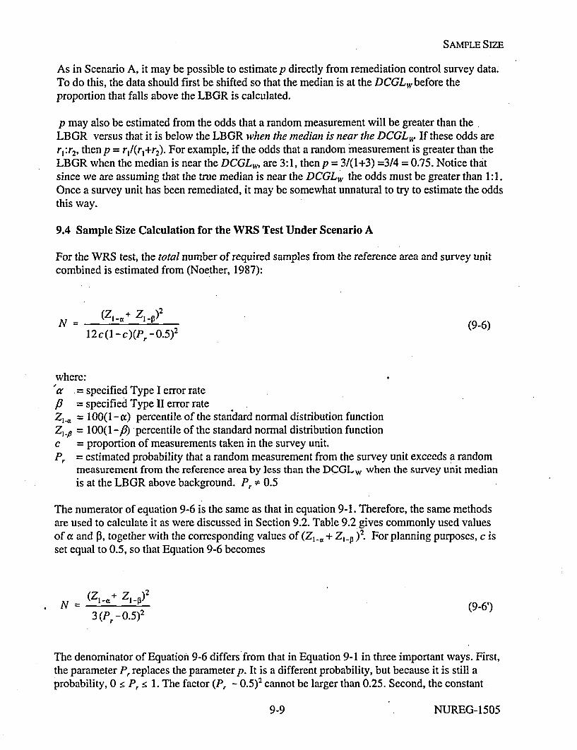
SAMPLE SIZE
As in Scenario A, it may be possible to estimate p directly from remediation control survey data.To do this, the data should first be shifted so that the median is at the DCGLw before theproportion that falls above the LBGR is calculated.
p may also be estimated from the odds that a random measurement will be greater than theLBGR versus that it is below the LBGR when the median is near the DCGL , If these odds arer,:r2, then p = rl/(r,+r2). For example, if the odds that a random measurement is greater than theLBGR when the median is near the DCGLW are 3:1, then p = 3/(1+3) =3/4 = 0.75. Notice thatsince we are assuming that the true median is near the DCGL1 v the odds must be greater than 1:1.Once a survey unit has been remediated, it may be somewhat unnatural to try to estimate the oddsthis way.
9.4 Sample Size Calculation for the WRS Test Under Scenario A
For the WRS test, the total number of required samples from the reference area and survey unitcombined is estimated from (Noether, 1987):
N (Z- 1 .+ Z 1 -))2 (9-6)12 c (I - c) (P,. - 0.5)(96
where:= specified Type I error rate
8 = specified Type II error rateZi.a= 100(l -a) percentile of the standard normal distribution functionZ1,6= 100(1 -,g) percentile of the standard normal distribution functionc proportion of measurements taken in the survey unit.P,= estimated probability that a random measurement from the survey unit exceeds a random
measurement from the reference area by less than the DCGLw when the survey unit medianis at the LBGR above background. Pr t 0.5
The numerator of equation 9-6 is the same as that in equation 9-1. Therefore, the same methodsare used to calculate it as were discussed in Section 9.2. Table 9.2 gives commonly used valuesof a and P3, together with the corresponding values of (Z,- + Z,•_ ). For planning purposes, c isset equal to 0.5, so that Equation 9-6 becomes
,N =(ZI-,+ Zl-P)2 (9-6')
3 (Pr - 0.5)2
The denominator of Equation 9-6 differs from that in Equation 9-1 in three important ways. First,the parameter Pr replaces the parameter p. It is a different probability, but because it is still aprobability, 0 < P•r 1. The factor (Pr - 0.5)2 cannot be larger than 0.25. Second, the constant
9-9 NUREG-1505
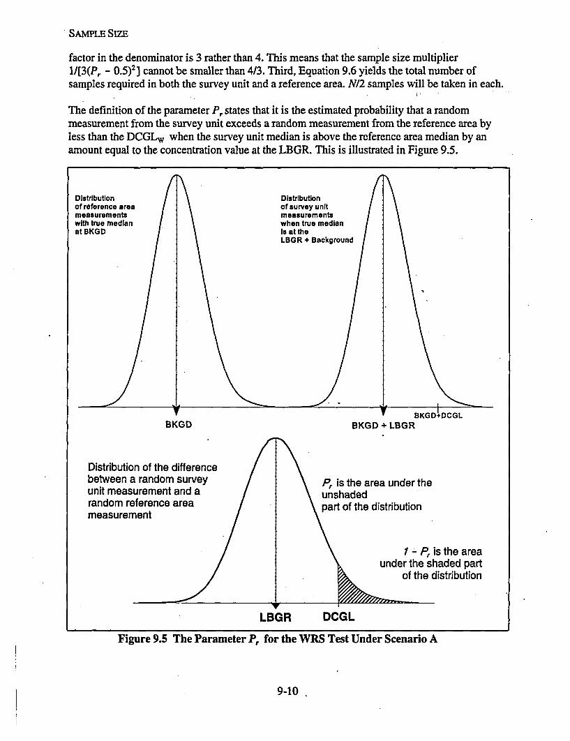
. SAMPLE SIZE
factor in the denominator is 3 rather than 4. This means that the sample size multiplier11[3(Pr - 0.5)2] cannot be smaller than 4/3. Third, Equation 9.6 yields the total number ofsamples required in both the survey unit and a reference area. N12 samples will be taken in each.
The definition of the parameter P, states that it is the estimated probability that a randommeasurement from the survey unit exceeds a random measurement from the reference area byless than the DCGLw when the survey unit median is above the reference area median by anamount equal to the concentration value at the LBGR. This is illustrated in Figure 9.5.
Distributionof reference areameasurementswith true medianatBKGD
Distributionof survey unitmeasurementswhen true medianIs at theLBGR + Background
;GLBKGD BKGD + LBGR
Distribution of the differencebetween a random surveyunit measurement and arandom reference areameasurement
P. is the area under theunshadedpart of the distribution
1 - P, is the areaunder the shaded part
of the distribution
V
LBGR DCGL
Figure 9.5 The Parameter P, for the WRS Test Under Scenario A
9-10

SAMPLE SIZE
As was done for the Sign test, the normal distribution may be used to facilitate the conversion ofthe values of A/c to values of Pr in order to calculate the required sample sizes. The normaldistribution is not used to actually conduct the test. Values of P, are computed for a normaldistribution from the following equation:
Pr -Probability(U=X - Y < DCGL)
Sfcj ffx( + y)f$(y)dydu
=Djffe -(ueY-LBGR)2D2 ed
12r f e -(u-LlGR) 21402 du
DCGLw-LBGR
1__. f e-X12dX
f
D( (9-7)
Values of Pr as a function of A/c are listed in Table 9.4. The probability P, and the sample sizemultiplier 1/[3(Pr - 0.5)2] are shown as a function of A/a in Figure 9.6.
Table 9.4 Values of P, for Use in Computing Sample Size for the WRS Test
A/o P, A/o P, A/o P,7 A/a P,
0.1 0.528186 1.1 0.781662 2.1 0.931218 3.1 0.9858110.2 0.556231 1.2 0.801928 2.2 0.940103 3.2 -0.9881740.3 0.583998 1.3 0.821015 2.3 0.948062 3.3 0.990188
0.4 0.611351 1.4 0.838901 2.4 0.955157 3.4 0.9918950.5 0.638163 1.5 0.855578 2.5 0.961450 3.5 0.9933360.6 0.664313 1.6 0.871050 2.6 0.967004 4.0 0.997661
0.7 0.689691 1.7 0.885334 2.7 0.971881 5.0 0.9997960.8 0.714196 1.8 0.898454 2.8 0.976143 6.0 0.999989
0.9 0.737741 1.9 0.910445 2.9 0.9798481.0 0.760250 2.0 0.921350 3.0 0.983053
9-11 NUREG-1505
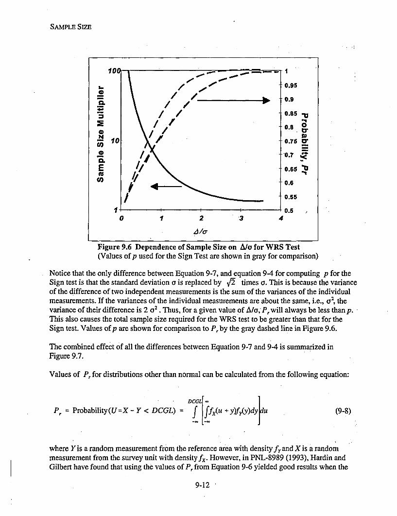
SAMPLE SIZE
10 .- ~1
/ - 0.95/ / , 0.9-/ / o0.85
0.80
N W-10 5 0.75 Cr
.2 1~0.7
/ 0.6
/ 0.55I I J 0.5
0 1 2 3 4
- ~A/o-
Figure 9.6 Dependence of Sample Size on A/a for WRS Test(Values of p used for the Sign Test are shown in gray for comparison)
Notice that the only difference between Equation 9-7, and equation 9-4 for computing p for theSign test is that the standard deviation Y is replaced by VF2 times a. This is because the varianceof the difference of two independent measurements is the sum of the variances of the individualmeasurements. If the variances of the individual measurements are about the same, i.e., 02, thevariance of their difference is 2 o2 . Thus, for a given value of A/a, Pr will always be less than p.This also causes the total sample size required for the WRS test to be greater than that for theSign test. Values of p are shown for comparison to P, by the gray dashed line in Figure 9.6.
The combined effect of all the differences between Equation 9-7 and 9-4 is summarized inFigure 9.7.
Values of Pr for distributions other than normal can be calculated from the following equation:
DCG4.o
Pr Probability(U=X - Y < DCGL) f.ffx(U + y)fr(yYU (9-8)
where Y is a random measurement from the reference area with density fy and X is a randommeasurement from the survey unit with densityfx. However, in PNL-8989 (1993), Hardin andGilbert have found that using the values of P, from Equation 9-6 yielded good results when the
9-12

SAMPLE SIZE
distributions being tested were positively skewed, such as the log-normal.
3
2.5;20
1a .5 -=) 1 -'---.
N - m••m
a$.5 Survey Unit Only
EM 0 1 2 3 4
Cl)A/a
Figure 9.7 Comparison of Sample Sizes Required for the WRS Test and the Sign Test
In some situations, it may be possible to estimate P,, directly from remediation control surveydata. It is an estimate of the proportion of time that a random survey measurement will exceed arandom reference area measurement by less than the DCGLw.
P, may also be estimated by the odds that a random survey measurement will exceed a randomreference area measurement by less than the DCGLwversus that a random survey measurementwill exceed a random reference area measurement by more than ihe DCGL w'. If these odds arer,:r2 , then Pr = r,1/(r, + r2).
Whatever method is used to estimate P., it is important not to overestimate it, since that willresult in a sample size inadequate to achieve the desired power of the test. The dependence of thesample size multiplier, 1/[3(Pr - 0.5)2], on Pr is shown in Figure 9.8.
As an illustration, consider the example given in Chapter 6.1. For that example, theDCGLW = 160, the LBGR = 142, a = P3 =0.05, and a = 6. From Table 9.2,(Z1_- + Z,.p )2 = 11when a = = 0.05. The width of the gray region, A = DCGLW - LBGR = 160 - 142 = 18, soA/o = 18/6 = 3.
From Table 9.4, thevalue of Pr using the normal approximation is 0.983053. Thus the factor1/[3(p - 0.5)2 ] = 1/[3(0.983053 - 0.5)2 ]
9-13 NUREG-1505

SAMPLE SIZE
= 1/[3(0.483053)2]= 1/[3(0.233340)]= 1/0.700021= 1.43.
So, the minimum sample size of 11 is increased by a factor of 1.43 to 15.7. This would normallybe rounded up to 16, or 8 samples each in the reference area and the survey unit. However,because Equation 9-6 is an approximation, it is prudent to increase this number moderately. Anincrease of 20% is recommended. This increases the number of samples to 1.2(15.7) = 18.9,which is rounded up to the next even integer, 20. Thus, 10 samples each in the reference areaand the survey unit are required. This is the number that appears in Table 3.3.
1000
100
10Coa..
E0.
0.5 0.6 0.7 0.8 0.9 1
pr
Figure 9.8 Dependence of Sample Size on P,
9.5 Sample Size Calculation for the WRS Test Under Scenario B
Under Scenario B, Equation 9-6 is also used to estimate the required sample size. The roles of aand P3 are reversed, but this has no effect on the numerator of Equation 9-6, so Table 9.2 may stillbe used. However, since under Scenario B, both the WRS test and the Quantile test are used intandem, the value of cc decided on during the DQO process is halved for each test. Thus, theTable 9.2 value for aw = a/2 and 03 is used.
The form of the denominator also remains the same, and Figure 9.8 still represents thedependence of the sample size multiplier on P,. However, the definition of the parameter P, isdifferent. The definition of the parameter Pr under Scenario B is the estimated probability thatthe difference between a random measurement from the survey unit and a random measurementfrom the reference area will be greater than the LBGR when the survey unit median is actually atthe DCGLw above the background median. This is illustrated in Figure 9.9.
9-14

SAMPLE SIZE
Distributionof reference areameasurementswith true medianat BKGD
Distributionof survey unitmeasurementswhen true medianis at theDCGL + BKGD
BKOD +LBORBKGD BKGD+DCGL
Distribution of the differencebetween a random survey unitmeasurement and a randomreference area measurement
P, is the area under the unshadedpart of the distribution
1 - P, is the area underthe shaded part of thedistribution IJ
-q ur
LBGRV
DCGL
Figure 9.9 The Parameter P, for the WRS Test Under Scenario B
The.value of 1 -P, expresses the likelihood that differences less than the LBGR will be observed,even if-half of the survey unit concentration distribution is above the background median bymore than the DCGLw. This likelihood is higher when the measurement standard deviation is
I
9-15 NUREG-1505

SAMPLE SIZE
large compared to the width of the gray region.
If, as in Scenario A, we assume that the data are approximately normally distributed, the width ofthe gray region, A/a = (DCGLw - LBGR)l/, can be used to estimate the parameter P,:
Pr = Probability(U =X - Y > LBGR)
LBGR[.O +Yf(dYU
1. -(u y-DCGLw-BKGDI2 12 2 -(y-BKGDo) 2I2dy2 u
= GR[f e 2 7ja
1 e -(u-DCGLW)14o2 du
DCGLw-LBGR
f-1 e -x212dx
=~z~ V2 4 (9-9)
This is the same as Equation 9-7. Even though the definition of Pr has changed, its value as afunction of A/u has not changed. Therefore, the value of Pr computed from Equation 9-7, asfound in Table 9.4, can be used in Scenario B as well as in Scenario A. Figure 9.6, expressingthe dependence of sample size on A/a is unchanged, and that is why only one version of Table3.3 is needed for both scenarios.
Values of P, for distributions other than normal can be calculated from the following equation:
r=Probability (U =X - Y > LBGR) = f [ffx(u + y)fy(.y)dy dA (9-10)
where Y is a random measurement from the referenece area with density fy and X is a randommeasurement from the survey unit with densityfx. ""
9-16

SAMPLE SIZE
As in Scenario A, it may be possible to estimate P, directly from remediation control survey data.To do this, the data should first be shifted so that the median is at the DCGLw before theproportion that fall above the LBGR is calculated.
Pr may also be estimated from the odds that a random measurement will be greater than theLBGR versus that it is below the LBGR when the median is near the DCGLw If these odds arerl:r 2, then Pr = r1(rl+r2). For example, if the odds that a random measurement is greater than theLBGR when the median is near the DCGLw, are 3: 1, then Pr = 3/(1+3) =3/4 = 0.75. Notice thatsince we are assuming that the true median is near the DCGLw, the odds must be greater than1:1. However, once a survey unit has been remediated, it may be somewhat unnatural to try toestimate the odds this way.
9-17. NUREG-1505

10 POWER CALCULATIONS FOR THE STATISTICAL TESTS
10.1 Statistical Power and the Probability of Survey Unit Release
The concept of the statistical power of a test was introduced in Section 2.3.2. The use of thisconcept in optimizing the design of final status surveys was discussed in Section 3.8.1. Thepower of a statistical test is defined as the probability that the null hypothesis is rejected when itis false. It is 1- 3, where P3 is the Type II error of the test.
The statistical power will have different implications for survey unit release, depending onwhether Scenario A or B is used. The same information can be expressed slightly differently. Inthis report, it is expressed as the probability that the survey unit passes the statistical test, i.e., theresult of the test is the decision that the survey unit may be released.
The relationship between this probability and the Type I and Type II errors was given inTable 3.1. Figures 3.9 through 3.12 show this probability as a function of the true residualradioactivity concentration for selected values of a and P3 over a range of sample sizes. In manycases, it will be sufficient to check the curve in these figures that corresponds most closely to thesituation at hand. In the following sections, the assumptions made and the calculations performedin creating these figures are described.
10.2 Power of the Sign Test Under Scenario A
Recall that for the Sign test in Scenario A, the test statistic, S+, was equal to the number ofsurvey unit measurements below the DCGLw. If S+ exceeds the critical value k, then the nullhypothesis that the median concentration in the survey unit exceeds the DCGLw is rejected, i.e.,the survey unit passes this test. The probability that any single survey unit measurement fallsbelow the DCGLw is found from Equation 9-2 or 9-3. The probability that more than k of the Nsurvey unit measurements fall below the DCGLw 'is simply the following binomial probability:
N kIN [p]'[l.p]N= 1 _ ( N [p],[l _p]N-i 1 _ (D k-Npi =k+l "I F0 N__p (_. _p), (01
The indicated approximation is generally used when both Np and N(1 -p) are five or greater.(Z(z) is the cumulative standard normal distribution function given in Table A. 1.
Withp calculated as in Section 9.2, Equation 10-1 yields the probability that the null hypothesisis rejected when the true median of the residual radioactivity concentration in the survey unit is atthe LBGR. This is the power of the test at the.LBGR.
The probability, p(C), that any single survey unit measurement falls below the DCGLw when thesurvey unit median concentration is at any other value, C, can be determined by simply replacingthe value of the LBGR in Equation 9-2 with the value of C:
10-1 NUREG-1505

POWER
DCGLW
p(C) f e_(x_)n/2a2 dx
C + (DCGLw - C)1 f e -(x- C)/2c2dx
(DCGLW- C)a
f e -X 2/2 d
( (DCGLW Q (10-2)
Note that if C = DCGLw, p(C) = 0.5. The assumption of normality is not critical in the abovecalculations, since it is only being used to estimate the power. However, if a different distributionis considered more appropriate, Equation 9-3 can be used to calculate p(C).
When the value of p(C) from Equation 10-2 is inserted in Equation 10-1, we obtain theprobability that the null hypothesis is rejected at the concentration C. When C = DCGLw, thisprobability is the probability of a Type I error, a"). This calculation can even be performed forvalues of C greater than the DCGLw. The probability obtained is still the probability that thenull hypothesis is rejected, i.e., that the survey unit passes the test.
If the probability that the null hypothesis is rejected (calculated from Equation 10-1) is plottedagainst the concentration, C, the result is called a power curve. When the power calculation isperformed at the design stage, using an estimated value of o, it is called a prospective powercurve. When the calculation is performed after the survey, using the standard deviation of thesurvey unit measurements as an estimate of a, it is called a retrospective power curve.
To illustrate the construction of a power curve, consider the example of Chapter 5. The DCGLwfor this example was 15.9 and the LBGR was 11.5. The DQOs for a = P = 0.05 resulted in asample size of N = 21, using the estimate that a = 3.3. From Table A.3, the critical value for theSign test with N=21 and a = 0.05 is k = 14. This is all of the information necessary to constructthe prospective power curve. To construct the retrospective power curve, we use the standarddeviation of the measurement data, 9.5, as the estimate of a.
The results of these calculations are shown in Table 10.1 and Figure 10.1.
0 )The value of a actually obtained from Equation 10-1 should be close to that specified in the DQOs. Itmay not exactly equal that value when the sample sizes are small, since the critical value, k, can only take integervalues.
NUREG-1505 10-2

POWER
Table 10.1 Example Power Calculations: Sign Test Scenario A
Prospective RetrosDectiveC (DCGLw - C)/a p(C)) power (DCGLw - C)Io p(C) power
(Eq. 10-2) (Eq. 10-1) (EA. 10-2) (Eq. 10-1)0 4.82 1.0000 1.000 1.67 0.9525 1.0005 3.30 0.9995 1.000 1.15 0.8749 0.9896 3.00 0.9987 1.000 1.04 0.8508 0.9727 2.70 0.9965 1.000 0.94 0.8264 0.9428 2.39 0.9916 1.000 0.83 0.7967 0.8849 2.09 0.9817 1.000 0.73 0.7673 0.80210 1.79 0.9633 1.000 0.62 0.7324 0.67911 1.48 0.9306 1.000 0.52 0.6985 0.544
11.5 1.33 0.9082 '0.998 0.46 0.6772 0.45912 1.18 0.8810 0.991 0.41' 0.6591 0.39013 0.88 0.8106 0.914 0.31 0.6217 0.26214 0.58 0.7190 0.627 0.20 0.5793 0.15115 0.27. 0.6064 0.217 0.09 0.5359 0.076
15.9 0.00 " 0.5000 0.039 0.00 0.5000 0.03916 -0.03 0.4880 0.031 -0.01 0.4960 0.03617 -0.33 0.3707 0.001 -0.12 0.4522 0.01418 -0.64 0.2611 0.000 -0.22 0.4129 0.00519 -0.94 0.1736 0.000 -0.33 0.3707 0.00120 -1.24 0.1075 0.000 -0.43 0.3336 0.000
0.8 --
-0.6 -
0 4
0.4 --
0.2 Prospective 44
02 .... Retrospective 44
00 5 10 15 20
Concentration
Figure 10.1 Example Power Curves: Sign Test Scenario A
10-3 NUREG-1505

POWER
Notice that the increase of a due to a higher than anticipated measurement standard deviationcauses the retrospective power curve to differ considerably from the prospective power curve. InTable 3.3, we see that A/c = (15.9 - 11.5)/9.5 = 0.46 results in a much larger required samplesize (over 100) to achieve the desired power. Recall that in this example, S+ = 11, which issmaller than the critical value k = 14. Thus the null hypothesis was not rejected. The survey unitdid not pass. We now see that this might have been a consequence of having insufficient powerrather than the survey unit actually exceeding the release criterion. The lack of power was due tounderestimating the measurement variability.
10.3 Power of the Sign Test Under Scenario B
Recall that for the Sign test in Scenario B, the test statistic, S+, was equal to the number ofsurvey unit measurements above the LBGR. If S+ exceeds the critical value k, then the nullhypothesis that the median concentration in the survey unit is less than the LBGR is rejected, i.e.the survey unit does not pass. The probability that any single survey unit measurement fallsbelow the DCGLw, is found from Equation 9-4 or 9-5. The probability that more than k of the Nsurvey unit measurements fall above the LBGR is simply the following binomial probability:
N (N) [p]Y[l p]_ = 1- k (N) [p]'[a p]N_ - k _-Np(0-
i=k+l i=0 VNp (I -p)
The indicated approximation is generally used when both Np and N(1 -p) are five or greater.1'(z) is the cumulative standard normal distribution function given in Table A. 1.
With p calculated as in Section 9.3, this is the probability that the null hypothesis is rejectedwhen the true median of the residual radioactivity concentration in the survey unit is at theDCGLw. This is the power of the test at the DCGLw.
The probability, p(C), that any single survey unit measurement falls above the LBGR when thesurvey unit median concentration is at any other value, C, can be determined by simply replacingthe value of the DCGLw in Equation 9-4 with the value of C:
A1 f e_-(x_22d
0LBGR
1 f e -(x - C)92o2°dx
%• 0 (LBGR-C)+C
1 e _x212dx
Vfi2" LBGR -C
a
NUREG-1505 10-4
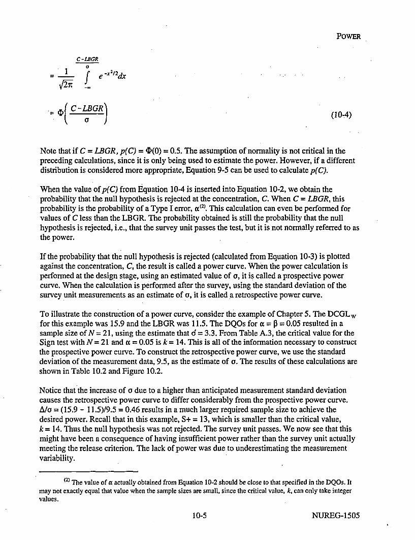
POWER
C -LBGR
-f ex 21dx
=((C~-LBGR) (10-4)
Note that if C = LBGR, p(C) 0 )(0) ; 0.5. The assumption of normality is not critical in thepreceding calculations, since it is only being used to estimate the power. However, if a differentdistribution is considered more appropriate, Equation 9-5 can be used to calculate p(C).
When the value of p(C) from Equation 10-4 is inserted into Equation 10-2, we obtain theprobability that the null hypothesis is rejected at the concentration, C. When C = LBGR, thisprobability is the probability of a Type I error, a(2). This calculation can even be performed forvalues of C less than the LBGR. The probability obtained is still the probability that the nullhypothesis is rejected, i.e., that the survey unit passes the test, but it is not normally referred to asthe power.
If the probability that the null hypothesis is rejected (calculated from Equation 10-3) is plottedagainst the concentration, C, the result is called a power curve. When the power calculation isperformed at the design stage, using an estimated value of a, it is called a prospective powercurve. When the calculation is performed after the survey, using the standard deviation of thesurvey unit measurements as an estimate of a, it is called a retrospective power curve.
To illustrate the construction of a power curve, consider the example of Chapter 5. The DCGLwfor this example was 15.9 and the LBGR was 11.5. The DQOs for a = P = 0.05 resulted in asample size of N = 21, using the estimate that d = 3.3. From Table A.3, the critical value for theSign test with N =21 and x = 0.05 is k = 14. This is all of the information necessary to constructthe prospective power curve. To construct the retrospective power curve, we use the standarddeviation of the measurement data, 9.5, as the estimate of a. The results of these calculations areshown in Table 10.2 and Figure 10.2.
Notice that the increase of a due to a higher than anticipated measurement standard deviationcauses the retrospective power curve to differ considerably from the prospective power curve.A/a = (15.9 - 11.5)/9.5 = 0.46 results in a much larger required sample size to achieve thedesired power. Recall that in this example, S+ = 13, which is smaller than the critical value,k = 14. Thus the null hypothesis was not rejected. The survey unit passes. We now see that thismight have been a consequence of having insufficient power rather than the survey unit actuallymeeting the release criterion. The lack of power was due to underestimating the measurementvariability.
(2) The value of a actually obtained from Equation 10-2 should be close to that specified in the DQOs. It
may not exactly equal that value when the sample sizes are small, since the critical value, k, can only take integervalues.
10-5 NUREG-1505
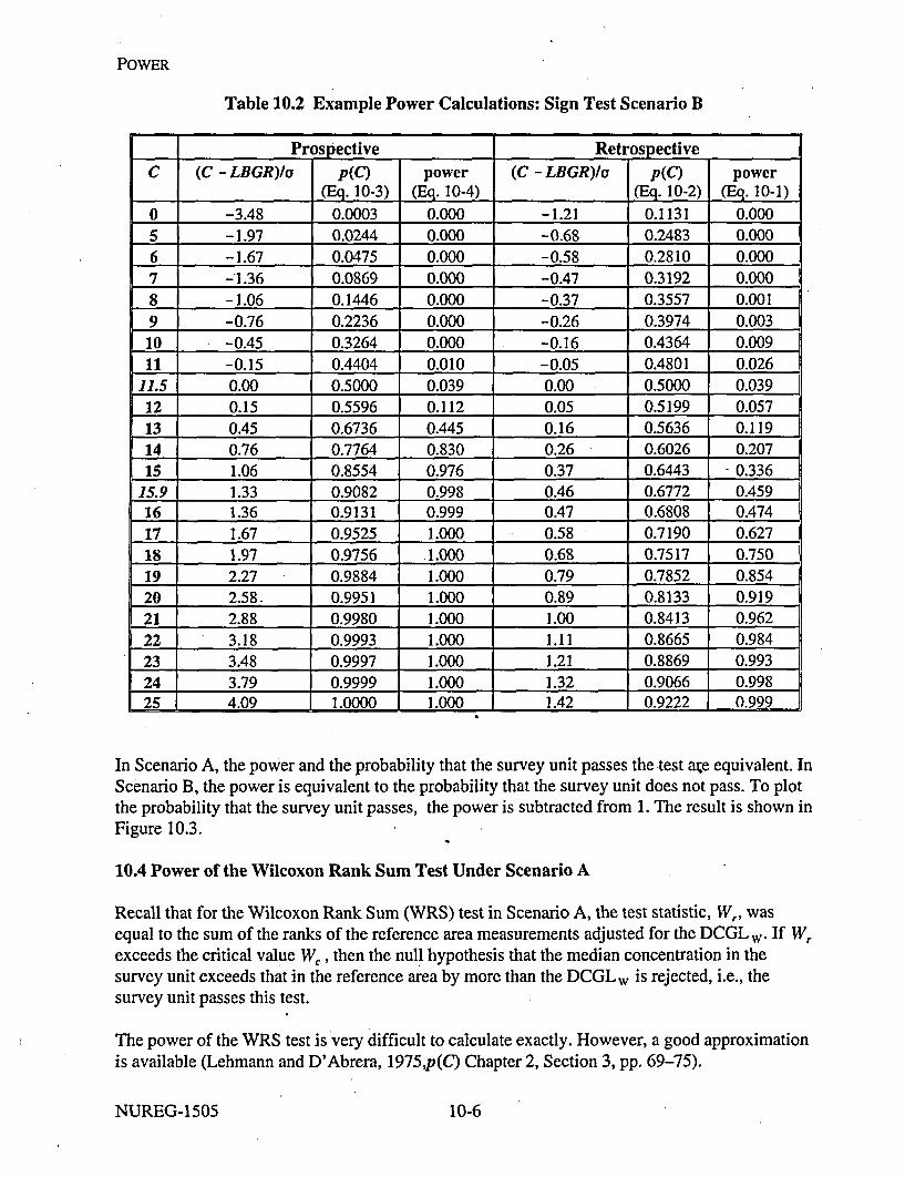
POWER
Table 10.2 Example Power Calculations: Sign Test Scenario B
Prospective Retrospective
C (C - LBGR)lu p(C) power (C - LBGR)lo p(C) power(Eq. 10-3) (Eq. 10-4) (Eq. 10-2) (Eq. 10-1)
0 -3.48 0.0003 0.000 -1.21 0.1131 0.0005 -1.97 0.0244 0.000 -0.68 0.2483 0.0006 -1.67 0.0475 0.000 -0.58 0.2810 0.0007 -1.36 0.0869 0.000 -0.47 0.3192 0.0008 -1.06 0.1446 0.000 -0.37 0.3557 0.0019 -0.76 0.2236 0.000 -0.26 0.3974 0.003
10 -0.45 0.3264 0.000 -0.16 0.4364 0.00911 -0.15 0.4404 0.010 -0.05 0.4801 0.026
11.5 0.00 0.5000 0.039 0.00 0.5000 0.03912 0.15 0.5596 0.112 0.05 0.5199 0.05713 0.45 0.6736 0.445 0.16 0.5636 0.11914 0.76 0.7764 0.830 0.26 0.6026 0.20715 1.06 0.8554 0.976 0.37 0.6443 0.336
15.9 1.33 0.9082 0.998 0.46 0.6772 0.45916 1.36 0.9131 0.999 0.47 0.6808 0.47417 1.67 0.9525 1.000 0.58 0.7190 0.62718 1.97 0.9756 1.000 0.68 0.7517 0.75019 2.27 0.9884 1.000 0.79 0.7852 0.85420 2.58. 0.9951 1.000 0.89 0.8133 0.91921 2.88 0.9980 1.000 1.00 0.8413 0.96222 3.18 0.9993 1.000 1.11 0.8665 0.98423 3.48 0.9997 1.000 1.21 0.8869 0.99324 3.79 0.9999 1.000 1.32 0.9066 0.99825 4.09 1.0000 1 .000 1.42 0.9222 0.999
In Scenario A, the power and the probability that the survey unit passes the test age equivalent. InScenario B, the power is equivalent to the probability that the survey unit does not pass. To plotthe probability that the survey unit passes, the power is subtracted from 1. The result is shown inFigure 10.3.
10.4 Power of the Wilcoxon Rank Sum Test Under Scenario A
Recall that for the Wilcoxon Rank Sum (WRS) test in Scenario A, the test statistic, W, wasequal to the sum of the ranks of the reference area measurements adjusted for the DCGLw. If Wrexceeds the critical value W,, then the null hypothesis that the median concentration in thesurvey unit exceeds that in the reference area by more than the DCGLw is rejected, i.e., thesurvey unit passes this test.
The power of the WRS test is very difficult to calculate exactly. However, a good approximationis available (Lehmann and D'Abrera, 1975,p(C) Chapter 2, Section 3, pp. 69-75).
NUREG- 1505 10-6

POWER
1.0
0.8
0.6
I. 0.4 /
/
0.2 Prospective
- - Retrospective /
00 5 10 15
Concentration
70/
//
I/
I
20 25
Figure 10.2 Example Power Curves: Sign Test Scenario B
1.00000
(A
MI.
0.0S
I-a.
0.4+
0.2Prospective
- - Retrospective
0 -- I I . . . . , I . 1 , 0 1 , I
0 5 10 15 20 25'
Concentration
Figure 10.3 Probability Example Survey Unit Passes: Sign Test Scenario B
10-7 NUREG-1505

POWER
If the distribution of the Mann-Whitney form of the WRS test statistic is approximated by anormal distribution, the probability that the null hypothesis will be rejected when the alternativeis true can be calculated from:
Power = -IP[W,-0.5 -O.5m(m+l)-E(10-5).lVarCWmw) (10-5)
where W, is the critical value found in Table A.4 for the appropriate values of the Type I error, a,the number of survey unit measurements, n, and the number of reference area measurements, m.E(WMw) and Var(WMw) are the mean and variance of the Mann-Whitney form of the WRS teststatistic. Values of (D(z), the standard normal cumulative distribution function, are given inTable A.1.
The Mann-Whitney form of the WRS test statistic is WMw = W, - 0.5m(m+ 1). It is obtained bysubtracting from Wr its minimum value, 0.5m(m+ 1). The mean of WMw is
E(WMw) = mnp, (10-6)
where p, is the probability that any single measurement from the survey unit exceeds a singlemeasurement from the reference area by less than the DCGLw. This probability depends on thedifference in median concentration between the survey unit and the reference area. When thisdifference is equal to the LBGR, then p, is equal to P, as calculated from Equation 9-7. For othervalues of the difference median concentration between the survey unit and the reference area, C,we simply replace the LBGR in Equation 9-7 with C:
P,(C) = Probability(U =X - Y < DCGL)
D DC1ffr( + yy)dy}du
fC 1 -(u.y-c-CBKGD) 2 2o2 I -(y-BKGDI 2 dyru
DCGL
1 f e _(uC)214 2du
VeV o
NUREG-1505 10-8

POWER
DCGLw- C
= 1 _•2 /2dx
= a V~(10-7)
Note that if C = DCGLw, then p(C) = 0.5. The assumption of normality is not critical in thepreceding calculations, since it is only being used to estimate the power. However, if a differentdistribution is considered more appropriate, Equation 9-8 can be used to calculate p I(C).
The variance of WMw is:
Var(WMw) = mnp1 (1 -p1 ) +mn(n-')(p2 -pr) +mn(m-1)(p3 -p2) (10-8)
P2 is the'probability that two random measurements from the survey unit will each exceed asingle random measurement from the reference area by less than the DCGLw; and P3iS theprobability that a single random measurement from the survey unit will exceed each of tworandom measurements from the reference area unit by less than the DCGLw. When thedifference in the concentration distributions of the survey unit and the reference areameasurements consists of a shift in the median, and the measurement distributions aresymmetric, then P2 = P3. Then the variance of Wmw simplifies to
Var(WMw) = mnpl(1-p,) +mn(n+m-2)(P2-Pr) (10-9)
If the measurement distributions are normal, then P2 is equal to the probability that two correlatedstandard normal random variables (i.e., with mean = 0 and variance = 1), with correlationcoefficient 0.5, are both less than (DCGLw - C)I(aV2-). This probability also depends on thedifference in median concentration, C, between the survey unit and the reference area. Even withthe simplifications employed, the values of p2'are not easy to calculate. Table 10.3 providesvalues of p, and P2 as a function of (DCGLw - C)/o that can be used in calculating the mean andvariance of Wmw. Nomographs of bivariate normal probabilities that can also be used for thispurpose are given in Abramowitz and Stegun (1972).
The power calculated using Equations 10-5 through 10-8 is an approximation. Thisapproximation was compared against the power simulations for the WRS test reported by Gilbertand Simpson (PNL-7409, 1992). It was found that the approximation is sufficiently accurate todetermine if the sample design achieves the DQOs.
10-9 NUREG-1505

POWER
Table 10.3 Values ofp, and P2 for Computing the Mean and Variance of WMW (3)
(DCGLw - C)Io Pi P2 (DCGLw - C)Io Pi P2
-6.0 0.000010 0.000000 0.7 0.689691 0.544073
-5.0 0.000204 0.000010 0.8 0.714196 0.574469
-4.0 0.002339 0.000174 0.9 0.737741 0.604402-3.5 0.006664 0.000738 1.0 0.760250 0.633702
-3.0 0.016947 0.002690 1.1 0.781662 0.662216
-2.5 0.038550 0.008465 1.2 0.801928 0.689800
-2.0 0.078650 0.023066 1.3 .0.821015 0.716331-1.9 0.089555 0.027714 1.4 0.838901 0.741698
-1.8 0.101546 0.033114 1.5 0.855578 0.765812-1.7 0.114666 0.039348 1.6 0.871050 0.788602
-1.6 0.128950 0.046501 1.7 0.885334 0.810016
-1.5 0.144422 0.054656 1.8 0.898454 0.830022
-1.4 0.161099 0.063897 1.9 0.910445 0.848605-1.3 0.178985 0.074301 2.0 0.921350 0.865767
-1.2 0.198072 0.085944 2.1 0.931218 0.881527
-1.1 0.218338 0.098892, 2.2 0.940103 0.895917-1.0 0.239750 0.113202 2.3 0.948062 0.908982
-0.9 0.262259 0.128920 2.4 0.955157 0.920777
-0.8 0.285804 0.146077 2.5 0.961450 0.931365
-0.7 0.310309 0.164691 2.6 0.967004 0.940817-0.6 0.335687 0.184760 2.7 0.971881 0.949208
-0.5 0.361837 0.206266 2.8 0.976143 0.956616-0.4 0.388649 0.229172 2.9 0.979848 0.963118
-0.3 0.416002 0.253419 3.0 0.983053, 0.968795
-0.2 0.443769 0.278930 3.1 0.985811 0.973725
-0.1 0.471814 .0.305606 3.2 0.988174 0.977981
0.0 0.500000 0.333333 3.3 0.990188 0.981636
0.1 0.528186 0.361978 3.4 0.991895 0.984758
0.2 0.556231 0.391392 3.5 0.993336 0.987410
0.3 0.583998 0.421415 4.0 0.997661 0.995497
0.4 0.611351 0.451875 5.0 0.999796 0.999599
0.5 0.638163 0.482593 6.0 0.999989 0.999978
0.6 0.664313 0.513387
When the values ofpI(C) and p2(C) and the resulting values of E(WMwv) and Var(WMw) areinserted in Equation 10-5, we obtain the probability that the null hypothesis is rejected atconcentration C. When C = DCGLw, this probability is the probability of a Type I error, a.
(3OThis table may also be used for Scenario B when (DCGLw - C)Io is replaced by (C - LBGR)Io.
(4) The value of a actually obtained from Equation 10-5 should be close to that specified in the DQOs. Itmay not exactly equal that value when the sample sizes are small, since the critical value, k, can only take integervalues.
NUREG-1505 10-10

POWER
The preceding calculations can even be performed for values of C greater than the DCGLW. Theprobability obtained is still the probability that the null hypothesis is rejected, i.e., that the surveyunit passes the test.
If the probability that the null hypothesis is rejected (calculated from Equation 10-5) is plottedagainst the concentration, C, the result is called a power curve. When the power calculation isperformed at the design stage, using an estimated value of a, it is called a prospective power•curve. When the calculation is performed after the survey, using the standard deviation of thesurvey unit measurements as an estimate of a, it is called a retrospective power curve.
To illustrate the construction of a power curve, consider the example of Chapter 6. The DCGLwfor this example was 160 and the LBGR was 142. The DQOs for a = = 0.05 resulted in asample size of n = m = 10, using the estimate that a = 6. Twelve samples each were actuallytaken from the survey unit and the reference area. From Table A.4, the critical value for the WRStest with n = m = 12 and a = 0.05 is W, = 179. This is all of the information necessary toconstruct the prospective power curve. To construct the retrospective power curve, we use thelarger of the standard deviations of the measurement data from the survey unit and the referencearea, 8. 1 as the estimate of a.
The results of these calculations are shown in Table 10.4 and Figure 10.4. In the figure it can beseen that the retrospective power is slightly less than that specified in the DQOs. However, inthis example, the null hypothesis was rejected, so the question of the power is moot. Theretrospective power calculation is really only necessary when the null hypothesis is not rejected.In that case, it is important to know that it was not rejected simply because there was insufficientpower. When the null hypothesis is rejected in spite of insufficient power, the survey designercan consider himself lucky, but the conclusion is still statistically valid.
Table 10.4 Example Prospective Power Calculation: WRS Test Scenario A
C (DCGLw - C)/o .P1 P2 E(WMw) Var(WMw) SD(Wuw) z Power
136 4.00 0.997661 0.995497 143.7 0.9 - 0.9 -46.21 1.00
139 3.50 0.993336 0.987410 143.0 3.2 1.8 -23.96 1.00
142 3.00 0.983053 0.968795 141.6 10.0 3.2 -12.98 1.00
145 2.50 0.961450 0.931365 138.4 27.4 5.2 -7.24 1.00
148 2.00 0.921350 0.865767 132.7 63.9 8.0 -4.02 1.00
151 1.50 0.855578 0.765812 123.2 124.9 11.2 -2.03 0.98
154 1.00 0.760250 0.633702 109.5 202.8 14.2 -0.63 0.74
157 0.50 0.638163 0.482593 91.9 271.9 16.5 0.52 0.30
160 0.00 0.500000 0.333333 72.0 300.0 17.3 1.65 0.05
163 -0.50 0.361837 0.206266 52.1 271.9 16.5 2.93 0.00
166 -1.00 0.239750 0.113202 34.5 202.8 14.2 4.63 0.00
169 -1.50 0.144422 0.054656 20.8 124.9 11.2 7.13 0.00
172 -2.00 0.078650 0.023066 11.3 63.9 8.0 11.15 0.00
10-11 NUREG-1505

POWER
1.0 S
N0.9--
0.8--
0.7
s.0.6-
00.50"
0.4--
0.3-- Prospective
0.2 --- - Retrospective0.1 •l•o':-• "
136 139 142 145 148 151 154 157 160 163 166 169 172
Concentration
Figure 10.4 Example Power Curves: WRS Test Scenario A
10.5 Power of the Wilcoxon Rank Sum Test Under Scenario B
Recall that for the WRS test in Scenario B, the test statistic, W5 , was equal to the sum of theranks of the survey unit measurements adjusted for the LBGR. If W, exceeds the critical valueWe, then the null hypothesis that the median concentration in the survey unit exceeds that in thereference area by less than the LBGR is rejected, i.e., the survey unit does not pass this test.
The power of the WRS test in Scenario B can be approximated in a manner similar to that usedin Scenario A, using Equations 10-5, 10-6 and 10-9:
Power, - 0.W-O5 -O'5m(m+I1)-- E(Wmw).
Power = 1 - Va
PiV&(mw)
E(WMw) = mnp,
Var(WMw) = mnp1(l -p 1) +mn(n+m-2)(p2 -p;)
NUREG-1505 10-12

POWER
W, is the critical value found in Table A.4 for the appropriate number of survey unitmeasurements, n, and number of reference area measurements, m. Since under Scenario B, boththe WRS test and the Quantile test are used in tandem, the value of the Type I error,' a, decidedon during the DQO process, is halved for each test. Thus, the Table A.4 value for value of W, foraw = a/2 is used. E(WMw) and Var(Wuw) are the mean and variance of the Mann-Whitney formof the WRS test statistic for Scenario B, namely WMW = W, - n(n+l)/2. Values of 4(z), thestandard normal cumulative distribution function, are given in Table A. 1.
In Scenario B, P, is the probability that any single measurement from the survey unit exceeds asingle measurement from the reference area by more than the LBGR . This probabilitydependson the difference in median concentration between the survey unit and the reference area. Whenthis difference is equal to the DCGLw, then p, is equal to P, as calculated from Equation 9-9. Forother values of the difference median concentration between the survey unit and the referencearea, C, we simply replace the DCGLw in Equation 9-9 with C:
Pr(C) Probability(U =X - Y > LBGR)
= + y)jfr(y)dy du
C -.fiBGR
_ 4 o f _x2 a2dx
= •( C-LBGR) (10-10)
This is the same as Equation 10-7, with (DCGLw - C) replaced by (C - LBGR). Although thedefinition of p, has changed, its value may still be found from Table 10.3 when (C - LBGR)Iois substituted for (DCGLw - C)Io. Note that if C = LBGR then p, (C) = 0.5. The assumption ofnormality is not critical in the above calculations, since it is only being used to estimate thepower. However, if a different distribution is considered more appropriate, Equation 9-10 can beused to calculate p,(C).
10-13 NUREG-1505

POWER
In Scenario B, P2 is the probability that two random measurements from the survey unit willeach exceed a single random measurement from the reference area by more than the LBGR; andp3 is the probability that a single random measurement from the survey unit will exceed each oftwo random measurements from the reference area unit by more than the LBGR. When thedifference in the concentration distributions of the survey unit and the reference areameasurements consists of a shift in the median, and the measurement distributions aresymmetric, then P2 = P3. If the measurement distributions are normal, then P2 is equal to theprobability that two correlated standard normal random variables (i.e., with mean = 0 andvariance = 1), with correlation coefficient 0.5, are both less than (C - LBGR)I(ovW ). Thisprobability also depends on the difference in median concentration, C, between the survey unitand the reference area. Again, values of P2 may be obtained from Table 10.3 when (C-LBGR)/ois substituted for (DCGLw - C)lo.
Although the power calculated as above is an approximation, this approximation has beencompared against the power simulations for the WRS test reported by Gilbert and Simpson(PNL-7409, 1992). It was found that the approximation is sufficiently accurate to determine if thesample design achieves the DQOs-
When the values of p,(C) and P2(C) from Table 10.3, and the resulting E(WMw) and Var(WMw) areinserted in Equation 10-5, we obtain the probability that the null hypothesis is rejected at theconcentration C. When C = DCGLw, this probability is the probability of a Type I error,
-w = a/2.(5). This calculation can even be performed for values of C less than the LBGR . Theprobability obtained is still the probability thai the null hypothesis is rejected, i.e., that the surveyunit passes the test, but it is not usually referred to as the power.
If the probability that the null hypothesis is rejected (calculated from Equation 10-5) is plottedagainst the concentration, C, the result is called a power curve. When the power calculation isperformed at the design stage, using an estimated value of a, it is called a prospective powercurve. When the calculation is performed after the survey, using the standard deviation of thesurvey unit measurements as an estimate of a, it is called a retrospective power curve.
To illustrate the construction of a power curve, consider the example of Chapter 6. The DCGLwfor this example was 160 and the LBGR was 142. The DQOs for cw = ad2 = 0.025, and P = 0.05,result in a sample size of n = m = 12, using the estimate that a = 6. From Table A.4, the criticalvalue for the WRS test with n = m = 12 and a = 0.025 is W, = 184. This is all of the informationnecessary to construct the prospective power curve. To construct the retrospective power curve,we use the larger of the standard deviations of the measurement data from the survey unit and thereference area, 8.1, as the estimate of a.
The results of these calculations are shown in Table 10.5 and Figure 10.5.
(5) Thd value of a actually obtained from Equation 10-5 should be close to that specified in the DQOs. Itmay not exactly equal that value when the sample sizes are small, since the critical value, k, can only take integervalues.
NUREG-1505 10-14
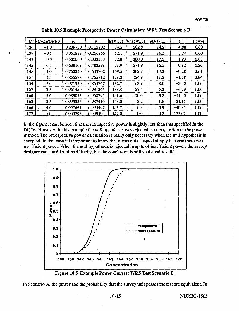
POWER
Table 10.5 Example Prospective Power Calculation: WRS Test Scenario B
C (C-LBGR)/o V p- E(W.uw) Var(W.;) SD(W.,W) z Power
136 -1.0 0.239750 0.113202 34.5 202.8 14.2 4.98 0.00139 -0.5 0.361837 0.206266 52.1 271.9 16.5 3.24 0.00142 0.0 0.500000 0.333333 72.0 300.0 17.3 1.93 0.03145 0.5 0.638163 0.482593 91.9 271.9 16.5 0.82 0.20148 1.0 0.760250 0.633702 109.5 202.8 14.2 -0.28 0.61151 1.5 0.855578 0.765812 123.2 124.9 11.2 -1.58 0.94154 2.0 0.921350 0.865767 132.7 63.9 8.0 -3.40 1.00157 2.5 0.961450 0.931365 138.4 27.4 5.2 -6.29 1.00160 3.0 0.983053 0.968795 141.6 10.0 3.2 -11.40 1.00163 3.5 0.993336 0.987410 143.0 3.2 1.8 -21.15 1.00166 4.0 0.997661 0.995497 143.7 0.9 0.9 -40.85 1.00172 5.0 0.999796 0.999599 144.0 0.0 0.2 -175.07 1.00
In the figure it can be seen that the retrospective power is slightly less than that specified in theDQOs. However, in this example the null hypothesis was rejected, so the question of the poweris moot. The retrospective power calculation is really only necessary when the null hypothesis isaccepted. In that case it is important to know that it was not accepted simply because there wasinsufficient power. When the null hypothesis is rejected in spite of insufficient power, the surveydesigner can consider himself lucky, but the conclusion is still statistically valid.
1.0
0.9.
0.8
0.7-
a0.6
00.5-
0.4.
0.3
0.2
0.1-
0,: II i : : II: iii III Ii: :
136 139 142 145 148 151 154 157 160 163 166 169 172
Concentration
Figure 10.5 Example Power Curves: WRS Test Scenario B
In Scenario A, the power and the probability that the survey unit passes the test are equivalent. In
10-15 NUREG-1505

POWER
Scenario B, the power is equivalent to the probability that the survey unit does not pass. Thus,the probability that the survey unit passes is one minus the power. The result is plotted in Figure10.6.
1.0-
0.9
Co0 0.8 " I
0.7
0.6-
0.5
0.4"°- Prospective
0.3 ,,,, " " Retrospectlv
O0.2--
0.1
0136 139 142 145 148 151 154 157 160 163 166 169 172
Concentration.
- Figure 10.6 Probability Example Survey Unit Passes: WRS Test Scenario B
.NUREG-1505 10-16

11 MULTIPLE RADIONUCLIDES
There are two cases to be considered when dealing with multiple radionuclides, namely (1) whenthe radionuclide concentrations have a fairly constant ratio throughout the survey unit, or (2)when the concentrations of the different radionuclides appear to be unrelated in the survey unit.In statistical terms, we are concerned about whether the concentrations of the differentradionuclides are correlated or not. A simple way to judge this would be to make scatter plots ofthe concentrations against each other, and see if the points appear to have an underlying linearpattern. The correlation coefficient can also be computed to see if it lies nearer to zero than toone. One could also perform a curve fit and test the significance of the result. Ultimately,however, sound judgment must be used in interpreting the results of such calculations. If there isno physical reason for the concentrations to be related, they probably are not. Conversely, if thereis sound evidence that the radionuclide concentrations should be related because of how theywere treated, processed or released, this information should be used.
11.1 Using the Unity Rule
In either of the two above cases, the unity rule described in Section 3.3 is applied. The differenceis in how it is applied. Suppose there are n radionuclides. If the concentration of radionuclide i isdenoted by Ci, and its DCGLw is denoted by Di, then the unity rule for the n radionuclides statesthat
C11D, + C21D2 + C31D3 + ... + C.ID,, • 1 (11-1)
This will ensure that the total dose due to the sum of all the radionuclides does not exceed therelease criterion. Note that if Dmin is the smallest of the DCGLs, then
(C1 + C2 + C3 + C,. )/Dmi. < C1ID, + C21D2 + C31D3 + ... + C.ID. (11-2)
So that the smallest DCGL may be applied to the total activity concentration, rather than usingthe unity rule. While it is an option to consider, in many cases this approach will be tooconservative to be useful.
11.2 Radionuclide Concentrations With Fixed Ratios
If there is an established ratio among the concentrations of the n radionuclides in a survey unit,then the concentration of every radionuclide can be expressed in terms of any one of them, e.g.,radionuclide #1. The measured radionuclide is often called a surrogate radionuclide for theothers.
If C2 = R2C1, C3 = R3C1, ..., Ci = RiC1 , ..., C, = RC,,CthenC11D, + C21D2 + C31D3 + - + C,.ID,, = C, ID, + R2C1 ID2 + R3C1 ID3 + ... + RC, ID,.
= C1 (lID 1 + R21D2 + R31D3 + ... + RID,.= CI/Dto, (11-3)
11-1 NUREG-1505

MULTIPLE RADIONUCLIDES
where
Dttal = 1/ [liD1 + R21D2 + R31D3 + + R,,ID,,]. (11-4)
Thus, DtotaI is the DCGLw for the surrogate radionuclide when the concentration of thatradionuclide represents all radionuclides that are present in the survey unit. Clearly, this schemeis applicable only when radionuclide-specific measurements of the surrogate radionuclide aremade. It is unlikely to apply in situations where the surrogate radionuclide appears inbackground, since background variations would tend to obscure the relationships between it andthe other radionuclides.
Thus, in the case in which there are constant ratios among radionuclide concentrations, thestatistical tests are applied as if only the surrogate radionuclide were contributing to the residualradioactivity, with the DCGLw for that radionuclide replaced by D1t0 . For example, in planningthe final status survey, only the expected standard deviation of the concentration measurementsfor the surrogate radionuclide is needed to calculate the sample size.
For the elevated measurement comparison, the DCGLEMC for the surrogate radionuclide is
replaced by
Etotd I=/ [lE, + R2 /E2 +R 3 IE3 + + Rn1En], (11-5)
where E, is the DCGLEMc for radionuclide i.
11.3 Unrelated Radionuclide Concentrations
If the concentrations of the different radionuclides appear to be unrelated in the survey unit, thenthere is little alternative to measuring the concentration of each radionuclide and using the unityrule. The exception would be in applying the most restrictive DCGLw to all of the radionuclides,as mentioned in Section 11.1.
Since the release criterion is
C1D 1 + C2 ID2 + C3 ID3 + ... + C/ ID, < 1.0 (11-6)
the quantity to be measured is the weighted sum, T = C1 ID, + C2 ID 2 + C3 ID3 + + Cn ID,.The DCGLw for T is 1.0. In planning the final status survey, the measurement standard deviationof the weighted sum, T, is estimated by
d(T) = [ 1( C)ID]2 + [o(C2)/D 2 2 + [0(C 3)ID 3 ] 2 + ... + [o([C.)ID ]2, (1 1-7)
since the measured concentrations of the various radionuclides are assumed to be uncorrelated.
For the elevated measurement comparison, the inequality .
C1/E1 + C21E2 + C3/E3 + ... + Cn/En < 1.0 (11-8)
NUREG-1505 11-2

MULTIPLE RADIONUCLIDES
is used, where E1 is the DCGLImc for radionuclide i. For scanning,' most restrictive DCGL.Mcshould generally be used.
When some of the radionuclides also appear in background, the quantityT = C, IDI + C21ID2 + C31ID3+ -. + C,, ID, "mustalso be measured in an appropriate reference area. If radionuclide i does not appear inbackground, set C1 = 0 in the calculation of T for the reference area.
Note that if there is a fixed ratio between the concentrations of some radionuclides, but notothers, a combination of the method of this section with that of the previous section may be used,using the appropriate value of Dtota, with the concentration of the measured surrogate radionuclideto replace the corresponding terms in Equation 11-7.
11.4 Example Application of WRS Test to Multiple Radionuclides
This section contains an example application of the nonparametric statistical methods in thisreport to sites that have residual radioactivity from more than one radionuclide. Consider a sitewith both WCo and 1"Cs contamination. `"7Cs appears in background from global atmosphericweapons tests at a typical concentration of about 1 pCi/g. Assume that the DCGLwfor To is 2pCilg and that for 131Cs is 1.4 pCi/g. In disturbed areas, the background concentration of '3aCscan vary considerably. An estimated spatial standard deviation of 0.5 pCi/g for `3Cs will beassumed. During remediation it was found that the concentrations of the two radionuclides werenot well correlated in the survey unit. 0Co concentrations were more variable than the '37csconcentrations, and 0.7 pCi/g is assumed for its standard deviation. Measurement errors for both6°Co and '37Cs using gamma spectrometry will be small compared to this. For the comparison tothe release criteria, the weighted sum of the concentrations of these radionuclides is computedfrom the following:
Weighted sum = (Co concentration)/(6WCo DCGLw) + (13'Cs concentration)/(' 37Cs DCGLW)
= (6°Co concentration)/(2) + ('37Cs concentration)/(1.4)
The variance of the weighted sum, assuming that the 6°Co and '37Cs concentrations are spatiallyunrelated is
a2 = [(60Co standard deviation)/(6°Co DCGLW)] 2 + [(137Cs standard deviation)/(' 37Cs DCGLw)]2
= [(0.7)/(2)]2 + [(0.5)/(1.4)]2 = 0.25.
Thus a = 0.5. The DCGLw for the weighted sum is one. Scenario A will be used, i.e., the nullhypothesis is that the survey unit exceeds the release criterion. During the DQO process, theLBGR was set at 0.5 for the weighted sum, so that A = DCGLw - LBGR =1.0 - 0.5 = 0.5, andA/a = 0.5/0.5 = 1.0. The acceptable error rates chosen were a = f3 = 0.05. To achieve this, 32samples each are required in the survey unit and the reference area.
The weighted sums are computed for each measurement location in both the reference area andthe survey unit. The WRS test is then performed on the weighted sum. The calculations for thisexample are shown in Table 11.1.
11-3 NUREG-1505

MULTIPLE RADIONUCLIDES
Table 11.1 Example WRS Test for Two Radionuclides
_ Reference Area Surve Unit Weighted Sum Ranks_ 37Cs 60Co 137Cs "Co Ref Survey Adj Ref Survey Adj Ref
1 2 0 1.12 0.06 1.43 0.83 2.43 1 56
2 1.23 0 1.66 1.99 0.88 2.18 1.88 43 21
3 0.99 0 3.02 0.56 0.71 2.44 1.71 57 14
4 1.98 0 2.47 0.26 1.41 1.89 2.41 23 55
5 1.78 0 2.08 0.21 1.27 1.59 2.27 9 50
6 1.93 0 2.96 0.00 1.38 2.11 2.38 37 54
7 1.73 0 2.05 0.20 1.23 1.56 2.23 7 46
8 1.83 0 2.41 0.00 1.30 1.72 2.30 16 52
9 1.27 0 1.74 0.00 0.91 1.24 1.91 2 24
10 0.74 0 2.65 0.16 0.53 1.97 1.53 27 6
11 1.17 0 1.92 0.63 0.83 1.68 1.83 13 18
12 1.51 0 1.91 0.69 1.08 1.71 2.08 15 32
13 2.25 0 3.06 0.13 1.61 2.25 2.61 47 63
14 1.36 0 2.18 0.98 0.97 2.05 1.97 30 28
15 2.05 0 2.08 1.26 1.46 2.12 2.46 39 58
16 1.61 0 2.30 1.16 1.15 2.22 2.15 45 41
17 1.29 0 2.20 0.00 0.92 1.57 1.92 8 25
18 1.55 0 3.11 0.50 1.11 2.47 2.11 59, 35
19 1.82 0 2.31 0.00 1.30 1.65 2.30 11 51
20 1.17 0 2.82 0.41 0.84 2.22 1.84 44 19
21 1.76 0 1.81 1.18 1.26 1.88 2.26 22 48
22 2.21 0 2.71 0.17 1.58 2.02 2.58 29 62
23 2.35 0 1.89 0.00 1.68 1.35 2.68 3 64
24 1.51 0 2.12 0.34 1.08 1.68 2.08 12 33
25 0.66 0 2.59 0.14 0.47 1.92 1.47 26 5
26 1.56 0 1.75 0.71 1.12 1.60 2.112 10 3827 1.93 0 2.35 0.85 1.38 2.10 2.38 34 53
28 2.15 0 2.28 0.87 1.54 2.06 2.54 31 61
29 2.07 0 2.56 0.56 1.48 2.11 2.48 36 60
30 1.77 0 2.50 0.00 1.27 1.78 2.27 17 4931 1.19 0 1.79 0.30 0.85 1.43 1.85 4 2032 1.57 0 2.55 0.70 1.12 2.17 2.12 42 40
Avg 1.62 0 2.28 0.47 1.16 1.86 2.16 Sum= Sum=
Std Dev 0.43 0 0.46 0.48 0.31 0.36 0.31 799 1281
In Scenario A, the DCGLw (i.e., 1.0) is added to the weighted sum for each location in thereference area. The ranks of the combined survey unit and adjusted reference area weighted sumsare then computed. The sum of the ranks of the adjusted reference area weighted sums is thencompared to the critical value for n = m = 32, a = 0.05, which is 1162 (see formula following
NUREG-1505 11-4.

MuLTIPLE RADiONUCLIDES
Table AA4). In Table 11.1, the sum of the ranks of the adjusted reference area weighted sums is1281. This exceeds the critical value, so the null hypothesis is rejected. The survey unit meets therelease criterion. The difference between the mean of the weighted sums in the survey unit andthe reference area is 1.86 - 1.16 = 0.7. Thus, the estimated dose due to residual radioactivity inthe survey unit is 70% of the release criterion.
11-5 NUREG-1505

t.

12 MULTIPLE SURFACES
12.1 Choosing Survey Units
Three criteria mentioned in Section 2.2 constrained the choice of survey units:
(1) Classification by Contamination Potential: Survey units are composed of areas with similarusage, contamination, and remediation histories that determine the requirements of the finalstatus survey.
(2) Congruity With the Dose Model Used: When the release criteria are dose-based, the surveyunit configuration should be consistent with those assumed in the dose model used.
(3) Data Variability: The measurement data variability, T, within survey units should beminimized so that acceptable decision error rates can be obtained with efficient sample sizes.
These criteria should guide the selection of survey units during the DQO process. However, thereare situations in which it will necessary to balance the requirements of one criterion against therequirements of another. In those circumstances, one should be guided by the ultimate objectiveof the final status survey, namely to make the correct decision on whether the survey unit meetsthe release criterion.
As an example, consider a room with a concrete floor, one wall with tile, another with wallboard,a third with glass doors and windows, and a fourth with a large blackboard. There are at least fivedifferent surfaces, with potentially five different levels of residual radioactivity. Using onlycriteria (1) and (3), it might seem important to treat these as five distinct survey units. However,this is not only very inefficient, it may not even be the best solution. It is unlikely that any dosemodel treats a contaminated blackboard by itself. Modeling the five areas separately andcombining the results may not be as faithful a representation as treating all the surfaces togetheras one contaminated room.
In this chapter, we discuss some of the factors to be considered during the DQO process tooptimize the choice of survey units. We also introduce the concept of performing a Sign test onpaired measurements when there are many diverse background materials present in a survey unit.
12.2 Combining Dissimilar Areas Into One Survey Unit
The primary disadvantages in separating very small areas of dissimilar contamination potentialinto distinct survey units are that such small survey units will not generally conform well to dosemodels, and that the resulting sample densities may be unreasonably high. The disadvantage ofcombining such areas is that the resulting survey unit will have a larger spatial concentrationvariability, requiring a larger sample size than if it were more uniform. However, the total samplesize may not be as large as would be needed for separate survey units. This possibility can beinvestigated and resolved during the DQO process.
12-1 12-I NUREG-1505

MULTIPLE SURFACES
Consider an area such as shown in Figure 12.1: a 25 m by 100 m gravel parking lot, with a pavedwalkway across a 25 m by 100 m lawn to a building. The walkway covers about 400 m2 of thelawn area. There are many ways that this area could be divided into survey units, depending onthe level of expected 'contamination.
Figure 12.1 Example Survey Units: Case #1
Example Case #1: 6Co was handled in hoods that were vented from the roof of the building.There is the possibility of a small amount of residual radioactivity, but at levels anticipated to befar below the DCGL. There is virtually no possibility of isolated elevated areas. All of the areaswould be considered Class 2. Surface samples will be analyzed for 'Co by Ge gammaspectrometry. The total area (5000 mi) is within the parameters used by the dose model.Although it is possible that average residual radioactivity levels between the walk, the gravel, andthe lawn are different, there is probably no reason to divide these areas into separate survey units.The walk may have almost no contamination because of runoff. Judgmental scans shouldprobably be made along the edges of the walk and along the side of the building.
Example Case #2: The same as example 1, except that there had been a spill in the gravel parkinglot. The area of the spill is shown as the dark area in Figure 12.2. During remediation of the spill,the surface material of the parking lot was disturbed by earthmoving equipment in thecrosshatched area, approximately 1700 n2. In this case, the disturbed area around the spillshould be considered a Class 1 area. The surrounding area is still Class 2. There is the possibilityof designating the entire parking lot as a Class 1 survey unit, but it might actually be morereasonable to include the uncontaminated part of the parking lot along with the other Class 2areas. This will yield a higher sampling density in the actual contaminated area, even though itincreases the variability in the Class 2 survey unit.
NUREG-1505 12-2
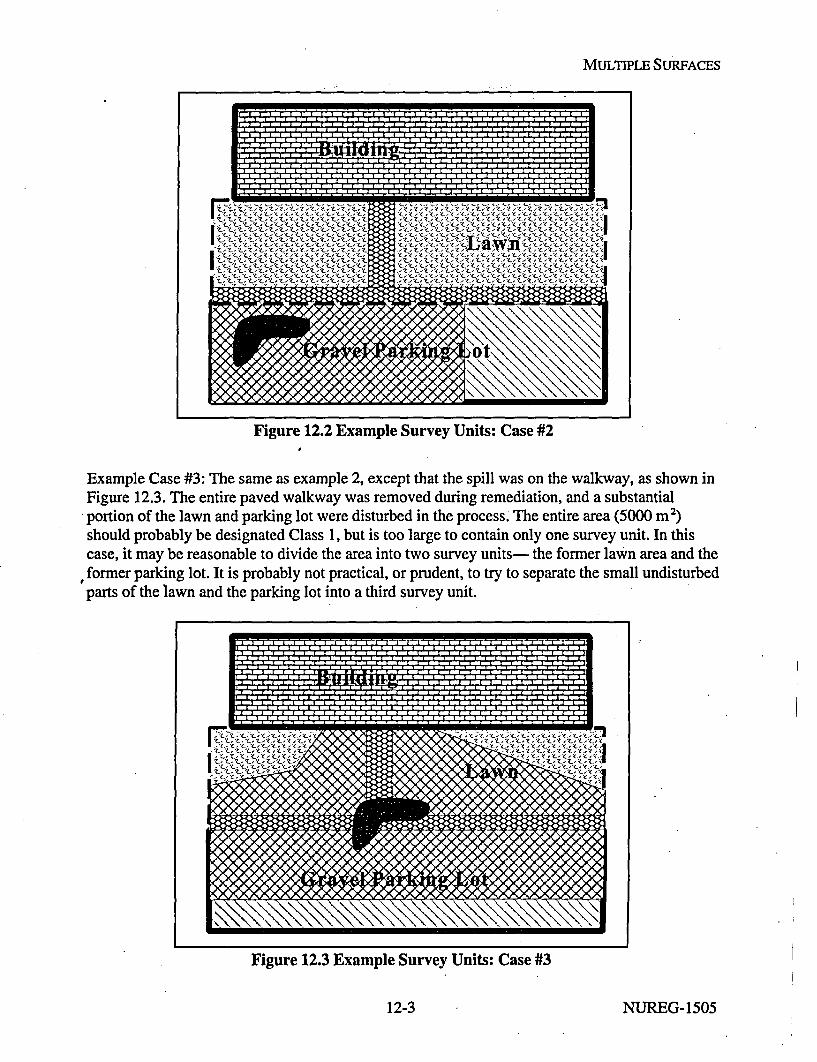
MULTIPLE SURFACES
Figure 12.2 Example Survey Units: Case #2
Example Case #3: The same as example 2, except that the spill was on the walkway, as shown inFigure 12.3. The entire paved walkway was removed during remediation, and a substantialportion of the lawn and parking lot were disturbed in the process. The entire area (5000 m2)should probably be designated Class 1, but is too large to contain only one survey unit. In thiscase, it may be reasonable to divide the area into two survey units- the former lawn area and the
f former parking lot. It is probably not practical, or prudent, to try to separate the small undisturbedparts of the lawn and the parking lot into a third survey unit.
------------ ------------
C~~~ _' (. -C C -C
Figure 12.3 Example Survey Units: Case #3
12-3 NUREG-1505

MULTIPLE SURFACES
These example cases are only meant to illustrate the considerations that may dictate how surveyunits may be designated, and what tradeoffs may be involved. What is actually done in anyspecific situation will depend on site-specific information from historical site assessments, andprior scoping, characterization, and remediation control survey results.
12.3 Using Paired Observations for Survey Units with Many Different Backgrounds
In this report, we have discussed using the Sign test for residual radioactivity that does not appearin background when radionuclide specific measurements are made, and otherwise using the WRStest. However, there are cases when one. may wish to use the Sign test even when theradionuclide appears in background and/or radionuclide specific measurements are not made. Anobvious instance would be when background is such a small fraction of the DCGL that includingit is unlikely to affect the decision errors. An example would be '37Cs residual radioactivity in anarea where the concentrations from global fallout are small. It may be more cost-effective tosimply compare the total 137Cs concentration in the survey unit to the DCGL using the Sign testrather than to attempt to find a matching reference area.
Another case in which the Sign test may be more appropriate is when there are many differentmaterials within what would otherwise logically be a single survey unit. As indicated at thebeginning of this chapter, to divide such a survey unit into separ.4te parts, each requiring its ownreference area is not only impractical, but may be inconsistent with the dose models used todetermine the DCGLs.
Consider once again, the example case #1 shown in Figure 12.1. Suppose the residualradioactivity of concern is 22.Ra rather than 'Co. We will call this example case #4. When 6Co
was the concern, only the variability in a material's potential for retaining or accumulating thisradionuclide was important. If 22.Ra is the concern, then the variability in the backgroundconcentration of 226Ra in the materials is an additional, perhaps more important concern informing survey units. In Figure 12.4, the same area as for case #1 is again shown, but withconsideration of this additional factor.
With an eye towards potential differences in background 226Ra, it becomes important that:" The walkway was paved with different concrete at two different times.* The parking lot was expanded using a different type of gravel.• Part of the lawn was graded with fill from another location.* Soil and mulch were used for the plant beds next to the building.
What were previously three potentially different survey units are now possibly as many as ninedifferent survey units. The contamination potential is still Class 2, as in case #1, and on that basisalone this area might be designated as a single survey unit. This disparity of effort between case#1, using the Sign test for 'Co, and case #4 using the WRS test for 226Ra is tremendous.
Fortunately, there is a third option- to use the Sign test with paired observations. Eachmeasurement in the survey unit is paired with an observation on a suitable reference material..The Sign test is then performed on the difference. The tradeoff is the higher variability of thedifferences compared to a single measurement.
NUREG-1505 12-4

MULTIPLE SURFACES
W ho ........
---------------------- ----- --X. . - . ..........................-'-Z , Xi
"t"L"t, Z.,Z X-
Figure 12.4 Example Survey Units: Case #4
In case #1, an estimate of the variability of the measurements from the survey unit, a, is neededto determine the relative width of the gray area, A/a, .which then in turn is used to determine therequired sample size, N. Suppose the survey unit measurements are designated by Y,, fori = I to N. From each of these Y1, a paired measurement, X,, on an appropriate reference materialis subtracted. The Sign test is performed on the difference Y1 - X,. Thus it is the variability ofthese differences, i -Xi), that is required in order to determine the required sample size. Thisvariability has three components:
G2 2 +2 2 2 + 2Y'-xI Yr °r X= (R + jB XO• (12-1)
where
oa, is the standard deviation of the measurements on the reference material,oy is the standard deviation of the measurements in the survey unit,aBi is the standard deviation of the background in the survey unit material, anda. is the standard deviation of the residual radioactivity in the survey unit.
If the reference material is truly representative, then oxi = oBi, so that
,2 , 2a =iXi a + 2 GBJ (12-2)
Better precision may be possible if the average of mjmeasurements made on thejth referencematerial is subtracted from each measurement from the survey unit made on that material.
The Sign test performed the differences:
12-5 NUREG-1505

MULTIPLE SURFACES
MY-j - in X (12-3)mi q=1
fork= 1 toni.
The variability of these differences is
O~'6 = +R + B ,Inj= OR +( nj) Osj (12-)
Note that when '°Co was the contaminant, the only component of variability was a = OR.
To estimate the sample size needed for case #1, suppose the DCGL for 'Co is 2 and that
OR = 0.7. If the LBGR is set at 1, then A/a = (2-1)/0.7 = 1.4. For acceptable error rates ofa = P = 0.05, the sample size found in Table 3.2 is 20. Suppose, for the sake of illustration, thatfor case #4, the DCGL for 226Ra is also 2, and oR = 0.7. If the 226Ra background standarddeviation is about 0.5, then standard deviation of the difference of matched pairs ofmeasurements,
°r-xj = aoR + 2o 7 = (0.7)2+ 2(0.5)2 = /0.49+ 0.5 = .99" 1 (12-5)
Thus, A/o = 1, and for the same LBGR of 1 and acceptable error rates of a = = 0.05, thesample size found in Table 3.2 is 29 measurements in the survey unit. An additional matching 29measurements on reference materials are also needed, for a total of 58 measurements. Tosimplify the above calculations, a single estimate of the standard deviation of backgroundmeasurements was used for all materials. It would be prudent to use the largest anticipatedstandard deviation. Note that no assumption about the average of the background concentrationsin the different materials was made. This may vary considerably from one material to another.
Indeed, if the average concentration does not vary significantly, it would be better to perform theWRS test using a. reference area with a composition that is reasonably well-matched to the surveyunit. Suppose in case #4, that the average concentrations of 226Ra did not vary much. Then thestandard deviation of background in the reference area is still about 0.5, and the variability in thesurvey unit is simply
= FR +2 = (0.7)2+ (0.5)2 = /0.49+ 0.25 -- .i 0.86 (12-6)
Thus, A/a = 1.155, and for the same LBGR of 1 and acceptable error rates of a = = 0.05, thesample size found by interpolating in Table 3.3 is about 26 measurements each required in the
NUREG-1505 12-6-

MULTIPLE SURFACES
survey unit and reference area for a total of 52 measurements. The WRS test requires fewermeasurements. An equivalent observation is that for the same number of measurements, theWRS test has greater power. The essential difference is whether the reference measurements canbe considered independent of the survey unit measurements, or whether they must be matchedtogether according to material type.
Notice that Equations 12-2, 12-4, and 12-6 differ primarily in the factor multiplying 0B . Using
the Sign test with a single matched reference measurement, this factor is 2. Using the WRS test,this factor is 1. If the mean of njmeasurements on the jth material is used this factor is (n, + 1)n/ j.This equals 2 when nj=l, and approaches 1 as njbecomes large.
The question remains as to how the measurements should be taken in the survey unit and fromthe reference materials. The measurements in the survey unit should be taken according to theregular procedure recommended for that class of survey unit, i.e., on a random start systematicgrid for Class 1 and Class 2, and randomly for Class 3. This is essentially the same as samplingaccording to the proportional area of each material in the survey unit. Matching reference areasamples should be taken randomly on the chosen reference material.
12-7 NUREG-1505

'a

13 DEMONSTRATING INDISTINGUISHABILITY FROM BACKGROUND
Thus far in this report the emphasis has been on conducting final status surveys that demonstratethat any residual radioactivity in a survey unit is within the release criterion. In these cases,Scenario A is generally preferred for the survey design. In some cases, however, it may be moreappropriate to demonstrate indistinguishability from background. Demonstrating Iindistinguishability from background using Scenario B will be a useful option when the residualradioactivity consists of radionuclides that appear in background, and the variability of thebackground is relatively high. Background variability may be considered high when differencesin estimated mean concentration measured in potential reference areas are comparable toscreening level DCGLs.
13.1 Determining Significant Background Variability
In Section 2.2.7, the concept of a reference area was introduced. Any difference in theconcentrations between the reference area and the survey unit is assumed to be due to residualradioactivity. It is not possible to determine whether or not an observed difference is actually dueto variations in the mean background concentrations between these areas.
When the variations in mean background among different potential reference areas are smallcompared to the width of the gray region, they can often be neglected. In such cases, the choiceof reference area will not materially affect the decision on whether or not to release a survey unitto which it is compared.
As the variations in mean background among different potential reference areas becomecomparable in magnitude to the width of the gray region, they can no longer be ignored. Whenthe reference area has a higher mean background than the survey unit, the survey unit will bemore likely to pass, and when the reference area has a lower mean bLackground than the surveyunit, the survey unit will be more likely to fail. Since any difference in background activitybetween the survey unit and the reference area is attributed to residual radioactivity, the choice ofreference area may materially affect the decision on whether or not to release a survey unit towhich it is compared.
As an example, consider Figure 13.1, which illustrates a DQO specification for a survey design.The gray region and acceptable rates for decision errors are shown by the solid curve. Supposethe reference area happens to have a lower mean concentration than the actual backgroundconcentrations in the survey unit. This difference is depicted by the double-headed arrow. Thevalues of residual radioactivity concentrations in this survey unit will appear larger than theyactually are by the amount of that difference. The result is that the actual probability that thesurvey unit passes is represented by the dashed curve, which is shifted downward from the solidcurve by the difference in mean background between the survey unit and the reference area. Thismeans, for example, that when the true residual radioactivity concentration is at the LBGR thereis only about a 65% probability of passing this survey unit, rather the 95% probability specifiedin the DQO.
Exactly how much, and in which direction the probabilities shift will depend on the particular
13-1 NUREG-1505

DEMONSTRATING INDISTINGUISHABILITY
reference area. Under such circumstances, whether a survey unit passes or fails may dependmore on the particular reference area chosen than on the amount of residual radioactivity that itcontains. This leads to a quantitative definition of what it means for a survey unit to beindistinguishable from background. It is expressed in terms of the potential for variations inreference area mean concentrations to impact decision error rates. First, it is necessary toestablish that there is significant variability among potential reference areas. A procedure fordoing this is discussed in the next section. If it shown that significant variability exists, thisinformation is used to define a level of residual radioactivity concentration that isindistinguishable from background variations. Section 13.4 discusses how this can be used toplan a final status survey using Scenario B.
1000
60 Probability of0passing Is
P lower If
= 40 -- reference -"
area mean Is.lower than
" 20 survey unit(U background
0a. 0
0 LBGR DCGL 1.5 DCGLTrue Concentration of Residual Radioactivity in Survey Unit
Figure 13.1 Impact of Background Variability on Decision Errors
13.2 Determining if Reference Areas Have Significantly Different Background Levels
In this section, we focus our attention on potential reference areas. Consider all the referenceareas to which a particular survey unit may be compared according to the criteria set out inSection 2.2.7. To determine whether there are significant differences among the reference areabackground means, the reference area measurements are expressed as:
xi = P'+ Zi+ (13-1)wherexUj= the jth measurement in the ith reference area, for j = 1 to n,, the number of measurements in
the ith reference area, and for i = 1 to k, the number of reference areas" = the mean concentration over all reference areas
pi = the difference between the overall mean and the mean in the ith reference areazU = the contribution of random spatial and measurement variability to the jth measurement in
the ith reference area
13-2 NUREG-1505

DEMONSTRATING INDISTINGUISHABILITY
is an unknown constant. The pi are distributed across reference areas with mean zero andstandard deviation c(, but within reference area i, pi has a fixed value. The z0 have mean zero andstandard deviation u. The measurements within reference area i have mean f+ pi, and varianceo2. The reference area means are distributed around the overall mean f with variance deviationW2. Thus, if there is no variability in the reference area means, then w2 0. The measurementvariability within each reference area is a2, and it is the same whether or not there is a significantdifference among the reference area means.
If the p, and the z are assumed to be normally distributed, the above corresponds to a randomeffects one-way analysis of variance model, sometimes called Model II. o2 and a2 are called thecomponents of variance. The null hypothesis, H0 : (.o2 = 0, versus the alternative, H.: Wo2 > 0, istested parametrically with an F-test. The non-parametric equivalent is the Kruskal-Wallis test.
Before collecting data for the Kruskal-Wallis test, the acceptable Type I error rate, a ,, must bespecified. This is the acceptable probability of concluding that the reference areas have differentaverage concentrations, when in fact they are the same. In setting a.n, it is important to considerthat the risk involved in a Type I error may be much smaller than the risk of a Type II error.
To perform the Kruskal-Wallis test, all of the measurements from the reference areas are pooledand ranked. For every measurement, x0, there is a corresponding rank, rj. There will beN = nj + n2 + ... + nk measurements in all. The sum of all of the ranks is N(N+I)12. Thereforethe average rank is N(N+I)l(2N) =(N+l)12. If the distribution of measured concentrations in eachreference area is the same, then the average rank for each reference area, should also be about thesame, i.e., (N+1)12.
Letn.
-i- E•_r R=Rni (13-2)nl, j=1
be the average rank in reference area i. The quantity R - (N+1)12 is a measure of howdifferent this reference area is from the others.
The Kruskal-Wallis statistic is a weighted sum of the squares of these differences over all of thereference areas:
N(N+I) n -(N+l)2 N(N 12 ( R52 1 ) - 3(N+l) (13-3)•J E = (j N N(N+I) i=I. 3(+1
The weights in Equation 13-3 have been chosen so that the probability that K exceeds a givenvalue K,, may be approximated by a chi-squared distribution with k-I degrees of freedom:
Prob(K > K) = 1 k- xk.m(K#) (13-4)
13-3 NUREG-1505

DEMONSTRATING INDISTINGUISHABILITY
2 2The critical value K, is determined from setting Xk-.(KC) = aCW. Values of XkI(K- ) for
typical values of ccw are tabulated in Table 13.1. If the value of K computed from Equation 13-3exceeds Kc, then the null hypothesis is rejected.
Table 13.1 Critical Values, K, for the Kruskal-Wallis Test
___aKW
k-1 0.01 0.025 0.05 0.1' 0.2
1 6.6 5.0 3.8 2.7 1.62 9.2 7.4 6.0 4.6 3.23 11.3 9.3 7.8 6.3 4.64 13.3 11.1 9.5 7.8 6.05 15.1 12.8 11.1 9.2 7.36 16.8 14.4 12.6 10.6 8.67 18.5 16.0 14.1 12.0 9.88 20.1 17.5 15.5 13.4 11.09 21.7 19.0 16.9 14.7 12.2
10 23.2 20.5 18.3 16.0 13.4
For example, suppose there are four reference areas under consideration, and ten measurementsare made in each. The data and the ranks are shown in Table 13.2. The same type of spreadsheetfunctions that were used for the WRS test can also be used to calculate the ranks for the Kruskal-Wallis test.
Using Equation 13-2,
K- 12 (_, Ri21n) - 3(N+l)N(N+I) 1
_ 12 (1552/10+1212/10+ 2 552/10+ 2 8 92/10 _ 3(41)40(41)
= 12 12- (2402.5+1464.1+6502.5+8352.1) - 123 = (18721.2) - 123.0 = 14.01640 1640
13-4 NUREG-1505

DEMONSTRATING INDISTINGUISHABILITY
With k-1 = 3, this value of K, is greater than the highest value of K, in Table 13.1, viz., 11.3 foraxw = 0.01 . The null hypothesis is rejected. It is concluded that these reference areas do havesignificantly different concentration distributions.
Table 13.2 Example Data for the Kruskal-Wallis Test
Measurements RanksAreal Area2 Area3 Area4 Areal Area2 Area3 Area4
1 0.27 1.04 2.45 3.77 6 13 27 39
2 1.87 0.39 0.34 2.63 1 20 9 8 313 0.97 2.07 3.06 4.05 10 23 37 40
4 1.01 -0.57 2.83 1.72 11 2 35 195 2.08 1.97 1.09 1.50 24 21 14 176 1.62 -0.22 0.26 2.47 18 3 5 29
7 0.30 1.39 2.80 1.42 7 15 34 16
8 1.98 0.05 2.77 2.47 22 4 33 28
9 2.18 -0.75 2.42 2.76 25 1 26 3210 1.02 2.50 2.86 3.35 12 30 36 38
Mean 1.33 0.79 2.09 2.61 Sum 155 121 255 289
StdDev 0.71 1.17 1.09 0.91 Total 820
13.3 Establishing the Concentration Level That Is Indistinguishable
Once it is decided that there are significant differences among the potential reference areas for a
survey unit, a measure of the variability among these reference areas is needed.
The sample mean of the measurements in area i is
ni
X, - (13-5)ni j=1
which provides an estimate of the mean concentration in reference area i, namely 'f+ Pii.
The overall sample mean
k ni
i=1 j=IEC
13-6)k
ni
13-5 NUREG-1505

DEMONSTRATING INDISTINGUISHABILITY
is an estimate of the overall mean background concentration, E.
The sample variance of the measurements in area i is
ni ni
si • (x - 1(n -1)= E (zi - 1(n, -1)j=1 j=1
(13-7)
which is an estimate of 02.
Since 02, is assumed to be the same in each reference area, these estimates can be pooled into thefollowing estimate:
SW k jn 1 1
(n1
i=1 j=I i=1
k
(=1
(13-8)
In the analysis of variance, s" is called the mean square within reference areas
The mean square between reference areas is
k kEni(pi -5ýC)2 nii-
2 ki- 1l i = l- k-i
± Xi) 2/ Etn,ki=lj=l i=1k-1
The righthand sides of Equations 13-8 and 13-9 may appear imposing, but essentially onlyinvolve:
(1) the sum of the squares of all the measurements,k ni
Ei(13-10)i=1 j=I
(1) The sum of the squared differences from the overall mean is composed of two parts:
k k n, k ni k n, k
E ~ (x x.-X) + E E. (5ý )2- L + xjF iX )i= j=I i=lj=l i=l j=l i=l j=l i=1
The first term on the right hand side is the sum of squares within reference areas and the second term on the righthand side is the sum of squares between reference areas. The mean square is obtained by dividing the sum ofsquares by the degrees of freedom. For the means square within reference areas this is the total number of datapoints minus the number of reference areas. For the means square between reference areas this is the number ofreference areas minus one.
13-6 NUREG-1505

DEMONSTRATING INDISTINGUISHABILITY
(2) the square of the sum of all the measurements,k nl \
and
(3) the sum of the squares of the reference area averages weighted by the number ofmeasurements,
k
i=l
The component of variance, c 2 , is estimated by
(13-11)
(13-12)
k
N - ni2 IN
where no = (k-i)0 (k-1)(Z2 2 2(b ( )no (13-13)
no is usually slightly less than the average number of samples taken in each reference area,'
kF = kI
k i=(13-14)
If the number of measurements in each reference area is the same, n I = n2 = ... = nk = n, then,
k
= (k-1)
_ N-kn2 IN(k-1)
kn - kn 2 Ikn(k-1)
kn -n
(k-1)_ n(k- 1)
(k-1)
(13-15)
The calculation of (Z2 for the example data of Table 13.2 proceeds using the sums and squares
shown in Table 13.3.
The sums (1), (2), and (3) together with Sb2 and sw 2 are calculated from Table 13.3 as follows:
From Equation 13-10,(1) = sum of squares = 22.28 + 18.50 + 54.30 + 75.80 = 170.88.
From Equation 13-11,(2) = square of the sum = (13.30 + 7.87 + 20.88 + 26.14)2= (68.19)2 =4649.88.
13-7 NUREG61505

DEMONSTRATING INDISTINGUISHABILITY
From Equation 13-12,(3) = weighted sum of the squares of the averages 10(1.332+ 0.792+ 2.092+ 2.612)
= 10(1.77 + 0.62 + 4.36 + 6.83) = 10(13.58) = 135.8.
From Equation 13-8,s.2 = (170.88 - 135.8)I(N-k) = (170.88 - 135.8)/36 = 0.97.
From Equation 13-9,
Sb2 = (135.8 - (4649.88/N))/(k- 1) = (135.8 - (4649.88/40))/(3) = 6.52.
Finally, we have
(s2 - Sw)Ino = (6.52 - 0.97)/10 = 0.55
Table 13.3 Calculation of 6' for the Example Data
(13-16)
Measurements Measurements SquaredArea 1 Area 2 Area 3 Area 4 Area 1 Area 2 Area 3 Area 4
1 0.27 -1.04 2.45 3.77 0.07 1.08 6.00 14.212 1.87 0.39 0.34 2.63 3.50 0.15 0.12 6.923 0.97 2.07 3.06 4.05 0.94 4.28 9.36 16.404 1.01 -0.57 2.83 1.72 1.02 0.32 8.01 2.965 2.08 1.97 1.09 1.50 4.33 3.88 1.19 2.256 1.62 -0.22 0.26 2.47 2.62 0.05 0.07 6.107 0.30 1.39 2.80 1.42 0.09 1.93 7.84 2.028 1.98 0.05 2.77 2.47 3.92 0.00 7.67 6.109 2.18 -0.75 2.42 2.76 4.75 0.56 5.86 7.62
10 1.02 2.50 2.86 3.35 1.04 6.25 8.18 11.22sum 13.30 7.87 20.88 26.14 22.28 18.50 54.30 75.80
average 1.33 0.79 2.09 2.61avg sqd 1.77 0.62 4.36 6.83
Although the analysis of variance using the F-test requires the assumption that the data are
normally distributed, the calculation of G.2 does not. Therefore, the values of the mean squares S2
and S 2 that are generated by most statistical computer programs for ANOVA can be used forthese calculations. Table 13.4 shows an ANOVA for the example data generated by a spreadsheetprogram. The entry for the mean square within groups, 0.97, is the same as was found in Table
13.3 for sW2. Similarly, the entry for the mean square between groups, 6.52, is the same as wasfound in Table 13.3 for Sb2. The F-statistic, which is simply the ratio Sb
2/Sw
2 , is also shown. Ofcourse, if the data from each reference area are consistent with the assumption of normality, theF-test may simply be used instead of the Kruskal-Wallis test.
13-8 NUREG-1505

DEMONSTRATING INDISTINGUISHABILITY
Table 13.4 Analysis of Variance for Example Data
Source of Sum of Degrees of Mean Square F StatisticVariation Squares Freedom
BetweenGroups 19.56 3 6.52 6.69WithinGroups 35.08 36 0.97
Total 54.65 39
13.4 Using the Concentration Level That Is Indistinguishable in the WRS Test
Recall from Section 3.6, that in Scenario B, the hypotheses being tested are
Null Hypothesis:HO: The mean concentration of residual radioactivity in the survey unit is indistinguishable from
background up to a level specified by the LBGR.versusAlternative Hypothesis:Ha: The mean concentration of residual radioactivity in the survey unit distinguishable from
background is in excess of the DCGLw.
In this scenario, a Type I decision error, with associated probability a, is made when a surveyunit fails when it should pass. A Type II decision error, with associated probability [3, is madewhen a survey unit passes when it should fail. To set these decision errors, an appropriate grayregion is needed. The lower bound on this gray region is the concentration level abovebackground that may be considered distinguishable from background.
If the null hypothesis of Kruskal-Wallis test has been rejected, the mean background levelsamong reference areas varies about the overall mean g with a standard deviation estimated by C,.-The difference in concentration that is distinguishable above background variability may beexpressed in terms of an appropriate multiple of 6). For example, if the reference area means arenormally distributed, the probability that the survey unit mean is more than two standarddeviations away from the overall mean is about 5%. Regardless of how the data are distributed,Chebyshev's Inequality states that the probability that the true mean background in the surveyunit differs from the overall mean background by more than t standard deviations is less than lit2.Therefore, the probability that the survey unit mean is more than t = 2 standard deviations awayfrom the overall mean is less than lt 2= 1/4 = 25%. The probability that the survey unit mean ismore than t = 3 standard deviations away from the overall mean is less than l1t2= 1/9 = 11%. Inmost cases, it is reasonable to assume that the true probabilities will fall somewhere between thevalue calculated for the normal distribution and that established by Chebyshev's inequality. Themultiple that of Ca that is used in a specific application should be decided during the DQOprocess, but a factor of three is a reasonable default.
13-9 NUREG-1505
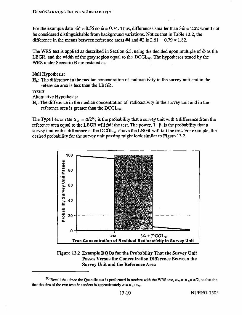
DEMONSTRATING INDISTINGUISHABIITY
For the example data W2 = 0.55 so C = 0.74. Thus, differences smaller than 36 = 2.22 would notbe considered distinguishable from background variations. Notice that in Table 13.2, thedifference in the means between reference areas #4 and #2 is 2.61 - 0.79 = 1.82.
The WRS test is applied as described in Section 6.3, using the decided upon multiple of 6) as theLBGR, and thewidth of the gray region equal to the DCGLw. The hypotheses tested by theWRS under Scenario B are restated as
Null Hypothesis:H0: The difference in the median concentration of radioactivity in the survey unit and in the
reference area is less than the LBGR.versusAlternative Hypothesis:Ha: The difference in the median concentration of radioactivity in the survey unit and in the
reference area is greater than the DCGL,
The Type I error rate caw = ac/2(2), is the probability that a survey unit with a difference from thereference area equal to the LBGR will fail the test. The power, 1 - P3, is the probability that asurvey unit with a difference at the DCGLw above the LBGR will fail the test. For example, thedesired probability for the survey unit passing might look similar to Figure 13.2.
100
80
60
40
C.
CL
0.o 20
36) 36) + DCGLw
True Concentration of Residual Radioactivity in Survey Unit
Figure 13.2 Example DQOs for the Probability That the Survey UnitPasses Versus the Concentration Difference Between theSurvey.Unit and the Reference Area
(2) Recall that since the Quantile test is performed in tandem with the WRS test, a w= a Q= a/2, so that the
that the size of the two tests in tandem is approximately a = aQ+aw
13-10 NUREG-1505

DEMONSTRATING INDISTINGUISHABILITY
The Quantile test is also performed as described in Section 7.2, with ccQ= ad2, and with theLBGR equal to the decided upon multiple of 6.
All of the reference area measurements taken for the Kruskal-Wallis test should also be used inthe WRS and Quantile tests. In most cases, no additional reference area samples will be needed.If additional samples are required, they should be obtained randomly, with all of the referenceareas being equally likely to be sampled.
13.5 Determining the Number of Reference Areas and the Number of Samples
In applying the methods of this chapter, it is natural to ask is how many reference areas should bestudied, and how many samples should be taken in each. As was seen in Section 3.8.1, thenumber of samples needed depends on both the probability of a Type I error (a) and theprobability of a Type II error (P3) that are deemed acceptable for the test. Unfortunately, the power(1-P) of the Kruskal-Wallis test involves functions that are "too complicated to be useful"(Lehmann and D'Abrerra, 1975). However, it has been shown that the efficiency of the Kruskal-Wallis test relative to the F-test is the same as the efficiency of the WRS test to the t-test(Andrews, 1954). This means that one can get an approximate idea of the power of the Kruskal-Wallis test by calculating the power of the F-test.The power of the F-test is (Brownlee, 1960, p.268):
1 -P = Probability[ F(fjf2) > F1-a-V114 2)A (13-17)
where
O2= 1 + n- ,and F1 -,(fJf 2) is the 1- aw percentile of the Fdistribution withf, = k - 1o2
andf2 = kn -k degrees of freedom. Through ý, the power depends on the ratio of the variancecomponents. Under the null hypothesis, C02 = 0, so (p = 1.
As an example, consider the data from Table 13.2. If one wished to detect a situation in which
W,2 = o22 then 4) =1+ 10(1)= 11. If aw= 0.1,then Fl_(flf 2) = F0.9(3,36) =2.243. The
power, 1- P3, is then the probability that the F-statistic with 3 and 36 degrees of freedom exceeds2.243/4 = 2.243/11 = 0.2039. P3 is the probability that the F-statistic with 3 and 36 degrees offreedom is less than 0.2039. This probability is about 13 = 0.1, so the power is about 0.9.
The results of this calculation for other numbers of samples and reference areas are shown inTable 13.5 for accw = 0.05, 0.10 and 0.20. Although this is only an approximation, and theactual power of the Kruskal-Wallis test would be slightly lower, this table indicates that with fourreference areas each with between 10 and 20 samples in each should generally be adequate. Sincethe risk of not detecting background variations that are actually present (a Type II error) couldinvolve the impossible task of remediating background, choosing a higher value for atv than forP would often be justified. From Table 13.5, when k = 4, this implies that aKW = 0.1 is areasonable default, and in some circumstances even larger values could be considered.
13-11 NUREG-1505

DEMONSTRATING INDISTINGUISHABILITY
Table 13.5 Power of the F-test When cw = a'
Number of Number Total 4) Power Power Powerreference of samples Number when when when
areas in each of a Kw = 0.05 a Kw = 0.1 a Kw = 0.2(k) (n) Samples
(kn) I
2 10 20 11 53.4% 60.7% 69.3%2 15 30 16 61.3% 67.4% 74.5%
2 20 40 21 66.1% 71.5% 77.7%2 30 60 31 72.1% 76.5% 81.7%3 10 30 11 74.0% 79.7% 85.7%3 15 45 16 81.8% 85.9% 90.1%3 20 60 21 86.1% 89.2% 92.4%
3 30 90 31 90.5% 92.7% 94.9%
4 10 40 11 85.3% 89.3% 93.0%4 15 60 16 91.4% 93.8% 96.0%
4 20 80 21 94.2% 95.8% 97.3%4 30 120 31 96.7% 97.6% 98.5%
5 10 50 11 91.8% 94.3% 96.5%
5 15 75 16 95.9% 97.2% 98.3%5 20 100 21 97.6% 98.4% 99.0%
5 30 150 31 98.9% 99.2% 99.5%
6 10 60 11 95.4% 97.0% 98.3%6 15 90 16. 98.1% 98.8% 99.3%
6 20 120 21 99.0% 99.4% 99.6%6 30 180 31 99.6% 99.8% 99.9%
13.6 Determining When Demonstrating Indistinguishability Is Appropriate
The methods of this chapter were developed specifically to address potential difficulties withdemonstrating compliance with dose-based release criteria at sites with spatially variablebackground concentrations of natural radionuclides. Generally, the use of Scenario A is preferredsince it involves fewer assumptions in its application and requires only one statistical test. Thenull hypothesis for Scenario A is such that when the residual radioactivity in the survey unit isvery close to the DCGLw, the default decision is to not release the survey unit without furtherinvestigation. This provides additional assurance that the release criteria will not be exceeded.However, when the variability in background is high, this assurance comes at too high a price,namely the possibility of requiring remediation of survey units containing only backgroundconcentrations of radionuclides. Since the default decision in Scenario B is to release the surveyunit, a second statistical test, the Quantile test, is used to detect non-uniform concentrations of
13-12 NUREG-1505

DEMONSTRATING INDISTINGUISHABILITY
residual radioactivity that may be excess of the release criterion, but that might be missed by theWRS test..
It is not possible to anticipate every circumstance in which these methods might be consideredapplicable. The suitability of these methods to specific situations should be determined duringthe DQO process. Two factors that should be considered in making this determination are:
(1) Have reasonable efforts been made to reduce measurement uncertainty. e.g., by use ofradionuclide-specific methods?
(2) Have reasonable efforts been made to reduce spatial variability by choosing homogeneoussurvey units with well-matched reference areas?
Once it is determined that the methods of this chapter are appropriate, the error rates for theKruskal-Wallis test should be set. The Kruskal-Wallis test is used to determine whether thespatial variability of average reference area background concentrations is significant. Thesignificance level is . If adequate consideration has been given to the decision to demonstrateindistinguishability, a-, need not be set to too low a value. Indeed, if it is felt that backgroundvariability should always have the benefit of the doubt, the Kruskal-Wallis test need not beconducted. Not conducting the test is essentially the same as setting a, = 1.0. Table 13.5 couldstill be used as a guide in determining the number of reference areas, and the number ofmeasurements in each, that will be used to estimate 6 according to the procedures ofSection 13.3.
Finally, the appropriate multiple of Z to be used as the LBGR should be determined. Thediscussion of this issue in Section 13.4 can be used as a guide.
13-13 NUREG-1505


14 ALTERNATIVES AND MODIFICATIONS
14.1 Alternative Statistical Tests
The nonparametric statistical tests described in this report are expected to perform well in a widevariety of circumstances. However, in some situations alternative methods can be considered. Asmentioned in Section 2.4.1, there are many statistical tests that can be used for determiningwhether or not a survey unit meets the release criteria. Any one test may perform better or worsethan others, depending on the hypotheses to be tested, i.e., the decision that is to be made and thealternative, and how well the assumptions of the test fit the situation. Some possible alternativesare discussed below.
In evaluating statistical tests, generally one chooses the test that has the highest power among thevarious alternatives. The power is compared when each test is set to have the same Type I errorrate, a. The Type I error rate is the probability that the null hypothesis will be rejected when it istrue. If the assumptions made about the data distribution are correct, the calculation of a formsthe basis for setting the critical value of the test statistic. If the assumptions are not valid, thecalculated value of a will differ from the true Type I error rate. The fewer assumptions that aremade, the more confidence can be placed in the calculation of the Type I error rate.
If a specific set of assumptions is made, the test results can be simulated using Monte Carlosampling techniques. Using a large number of simulations, the actual Type I and Type II errorrates for different tests can be compared. For each sample size, and specific set of assumptions, aseparate simulation must be performed. Although much can be learned about the relativeaccuracy of statistical tests in this way, it is clearly not possible to explore every potential set ofassumptions.
An alternative is to look at large sample results. With very few exceptions, it can be proved thatthe average of a large enough number of random data points tends to be normally distributed(Central Limit Theorem). In the same way, the power of statistical tests can be examined whenthe sample sizes are large enough. Note that what is meant by large enough is not preciselyspecified. Depending on the situation, large enough might be 10, or it might be 1000. If thesamples size is allowed to grow large enough, the asymptotic (i.e., in the limit of arbitrarily largesample size) behavior of tests can be compared. Better large sample test behavior may be takento imply that a test is better for all sample sizes. In reality, it can only be used as an indication ofwhich test might be preferred.
One measure commonly used to compare statistical tests is called the relative efficiency. This isdefined as the inverse of the ratio of sample sizes needed to achieve a given level of statisticalpower. If a test has relative efficiency of two relative to another, it requires half the sample sizeto achieve the same power. The asymptotic relative efficiency of one test to another, is the limitof the relative efficiency when the sample size is arbitrarily large.
14-1 NUREG-1505
ALTERNATIVES AND MODIFICATIONS
Wilcoxon Signed Ranks Test (WSR test)
The asymptotic relative efficiency of the WSR test compared to the Sign test can be greater orless than one. That is, either might be better, depending on the data distribution. The WSR testtends to be better when the data distribution is symmetric, and the Sign test tends to be betterwhen the data distribution is skewed.
Student's t-Test
Student's t-test may be used if the data have a nornial distribution. This is a more restrictiverequirement than that of symmetry, since every normal distribution is symmetric, but there aremany other distributions that are also symmetric. The assumption of normality should bechecked before using this test. The Shapiro-Wilk test discussed in EPAIQA-G9 (1996) is onesuch test. Others include the Kolmogorov-Smimov test, Lillifor's test, and the Chi-Squared test.
The asymptotic relative efficiency of the WSR test relative to the one-sample Student's t-testranges from 0.864 to infinity. As stated by Conover (1980): "the Wilcoxon test never can be toobad, but it can be infinitely good ... .. The asymptotic relative efficiency of the WRS testcompared to the two-sample Student's t-test has the same range, from 0.864 to infinity.
Chen's Test
Chen's test (Chen, 1995) is a modification of the Student's t-test that has been suggested for usewhen data are from a positively skewed distribution. Simulations show that it is generally morepowerful than other forms of the t-test. However, this test can only be used in Scenario B.
Lognormal Test
If the data are assumed to lognormal, the testing procedure of Land (1988) may be used. Theassumption of lognormality should be checked by testing the logarithms of the data for normality.It is important to note that a test on the mean of a lognormal distribution cannot be performed byusing a Student's t-test on the mean of the logarithms of the data. This is because the mean of thelogarithms of the data is the logarithm of the median of the original data. The behavior of thistest relative to others when the assumption of lognormality is violated has not been studied.
Bootstrap Methods
The bootstrap is a simulation technique (Efron and Tibshirani, 1993). In essence, the distributionof concentrations in a survey unit is approximated by the empirical distribution (e.g., histogram)of the sample data taken. If n measurements are made, these n measurements are randomlysampled n times with replacement. Each time this is done, the mean of the random sample iscalculated. After this has been done a specified number of times (generally between 50 and 200),the standard deviation of all of the random sample means is calculated. This is then used as theestimate of the standard error of the mean. There are, in addition, several methods for computingbootstrap t-statistics. Usually 1000 or more replications are recommended for the bootstrap t.Bootstrap methods generally have-good asymptotic properties, but can be sensitive to outliers,and erratic when sample sizes are small.
NUREG-1505 14-2

ALTERNATIVES AND MODIFICATIONS
14.2 Retesting
It may happen that a survey unit fails the hypothesis test (i.e., the decision is made that thesurvey unit does not meet the release criterion), yet the mean of the measured data is below therelease criterion. This is more likely to occur when the mean falls in the gray region thanotherwise. It analogous to the situation in which the mean is below the release criterion, but the1- ca upper confidence level on the mean falls above the release criterion. It may be that thesurvey unit does meet the release criterion, but the hypothesis test was not powerful enough todetect that with the number of samples taken. Under some circumstances, one might like theoption to take additional random samples and re-perform the hypothesis test on the entire set ofdata. The major difficulty with this is that the Type I error rate will now be greater than originallyspecified in the DQOs.
Sequential testing is performed when data are collected and analyzed in stages. It differs fromhypothesis testing in that at each stage a third alternative is added to the decision of whether ornot to reject the null hypothesis, namely, to collect more data before deciding. The usualmotivation for sequential testing is to reduce the expected total number of samples from thatrequired when all the sample are taken at one stage. Sequential versions of the WSR and WRStests are discussed by Spurrier and Hewett (1976).
14.3 Composite Sampling
The number of measurements taken in a Class 1 survey unit may sometimes be driven more bythe need to locate small areas of elevated activity than by the need to achieve the specifiedacceptable error rates for the statistical tests. When the scanning MDC is high, the sample size,N, may need to be significantly increased, in order to decrease the area between samples on thesystematic grid. When this grid area, about A/N, is small enough, so that in turn the area factor issufficiently high, the result is a DCGLEMC that is detectable by scanning. If the sample size N ismuch greater than that required for the statistical tests, some number, m, of neighboring samplesmight be composited to reduce the total cost of analysis. Suppose there are N = mnmeasurements. Each composite represents a contiguous area of approximately the sameproportion of the survey unit, m(A/N). The number of composite measurements, n, should beequal to or greater than the number of measurements required by the statistical test. When theelevated measurement comparison is performed against the composites measurement results, theDCGLEMC should be divided by the number of samples included in each composite. If thecomposite measurement is below DCGLEMc/m, no individual sample contributing to thecomposite could exceed the DCGLEMC.
If a composite measurement is flagged by the EMC, it may be necessary to reanalyze eachsample included in that composite to determine which of them, if any, actually exceed theDCGLEMC or, alternatively, the area of the survey unit represented by that compositemeasurement should be reinvestigated.
14-3 NUREG-1505

.J

15 GLOSSARY
Amin: The smallest area of elevated activity identified using the DQO Process that it is importantto identify.
action level: A scanning measurement level for residual radioactivity that (1) is based on theDCGL and (2) triggers a response, such as further investigation or cleanup, if exceeded. Seeinvestigation level.
activity: See radioactivity.
affected area: This term was previously used for areas that would be designated Class 1 orClass 2.
affected/non-uniform: This term was previously used for areas that would be designatedClass 1.
affected/uniform: This term was previously used for areas that would be designated Class 2.
ALARA (acronym for as low as is reasonably achievable): A basic concept of radiationprotection which specifies that exposure to ionizing radiation and releases of radioactivematerials should be reduced as far below regulatory limits as is reasonably achievableconsidering economic, technological, and societal factors, among others. Reducing exposure at asite to ALARA strikes a balance between what is possible through additional remediation and theuse of additional resources to achieve a lower level. A determination of ALARA is a site-specificanalysis that is open to interpretation, because it depends on approaches or circumstances thatmay differ between regulatory agencies. An ALARA recommendation should not be interpretedas a set limit or level.
alpha (a): The specified maximum probability of a Type I decision error, i.e., the maximumprobability of rejecting the null hypothesis when it is true. Alpha is also referred to as the size ofthe test. Alpha reflects the amount of evidence the decision maker would like to see beforeabandoning the null hypothesis.
alpha particle: A positively charged particle emitted by some radioactive materials undergoingradioactive decay.
alternative hypothesis (Ha): See hypothesis.
area: A general term referring to any portion of a site, up to and including the entire site.
area of elevated activity: An area over which residual radioactivity exceeds a specified valueDCGLEMc.
area factor (A.): A factor used to adjust DCGLw to estimate DCGLEMc and the minimumdetectable concentration for scanning surveys in Class 1 survey units -
15-1 NUREG-1505

GLOSSARY
DCGLEMc = (DCGLw)(Am). Am is the magnitude by which the residual radioactivity in a smallarea of elevated activity can exceed the DCGLw while maintaining compliance with the releasecriterion.
arithmetic mean: The average value obtained when the sum of individual values is divided bythe number of values.
arithmetic standard deviation: A statistic used to quantify the variability of a set of data. It iscalculated in the following manner: (1) subtracting the arithmetic mean from each data valueindividually; (2) squaring the differences; (3) summing the squares of the differences; (4)dividing the sum of the squared differences by the total number of data values less one; and (5)taking the square root of the quotient. The calculation process produces the Root Mean SquareDeviation (RMSD).
background radiation: Radiation from cosmic sources; naturally occurring radioactivematerial, including radon (except as a decay product of source or special nuclear material); andglobal fallout as it exists in the environment from the testing of nuclear explosive devices orfrom nuclear accidents which contribute to background radiation and are not under the control ofthe licensee. Background radiation does not include radiation from source, byproduct, or specialnuclear materials regulated by the NRC.
becquerel (Bq): The International System (SI) unit of activity equal to one nucleartransformation (disintegration) per second. 1 Bq = 2.7x101" Curies (Ci) = 27.03 picocuries(pCi).
beta (p): The probability of a Type 11 decision error, i.e., the probability of accepting the nullhypothesis when it is false. The complement of beta (1 -[3) is referred to as the power of the test.
beta particle: An electron emitted from the nucleus during radioactive decay.
bias: The systematic or persistent distortion of a measurement process which causes errors inone direction.
biased sample or measurement: See judgment sample or measurement.
byproduct material: Any radioactive material (except special nuclear material) yielded in ormade radioactive by exposure to the radiation incident to the process of producing or utilizingspecial nuclear material.
CEDE (committed effective dose equivalent): The effective dose equivalent is the summationof the products of the dose equivalent received by specified tissues of the body and a tissue-specific weighting factor. It is a risk-equivalent value, expressed in Sv or rem, that can be used toestimate the health effects on an exposed individual. See TEDE.
characterization survey: A type of survey that includes facility or site sampling, monitoring,and analysis activities to determine the extent and nature Of contamination. Characterization
NUREG-1505 ..15-2

GLOSSARY
surveys provide the basis for acquiring necessary technical information to develop, analyze, andselect appropriate cleanup techniques.
Class 1 area: Areas containing locations in which, prior to remediation, the concentrations ofresidual radioactivity may have exceeded the DCGLw.
Class 1 survey: A type of final status survey that applies to areas with the highest potential forcontamination. Class 1 surveys require (1) sufficient measurements on a systematic grid to meetthe desired error rates for the statistical hypothesis tests; (2) scanning over 100% of the surveyunit; (3) scanning MDC at or below the DCGLEMC.
Class 2 area: Areas containing no locations where, prior to remediation, the concentrations ofresidual radioactivity may have exceeded the DCGLw.
Class 2 survey: A type of final status survey that require (1) sufficient measurements on asystematic grid to meet the desired error rates for the statistical hypothesis tests; (2) judgmentalscanning of a portion, up to 100%, of the survey unit.
Class 3 area: Areas with a low probability of containing any locations with residualradioactivity.
Class 3 survey: A type offinal status survey that require (1) sufficient measurements atrandomly chosen locations to meet the desired error rates for the statistical hypothesis tests; (2)judgmental scanning over less than 10% of the survey unit.
classification: The act or result of separating areas or survey units into one of three designatedclasses: Class I area, Class 2 area, or Class 3 area.
composite sample: A sample formed by collecting several samples and combining them (orselected portions of them) into a new sample which is then thoroughly mixed.
confirmatory survey: A type of survey that includes limited independent (third-party)measurements, sampling, and analyses to verify the findings of afinal status survey.
contamination: The presence of residual radioactivity in excess of levels which are acceptablefor release of a site or facility.
criterion: See release criterion.
critical group: The group of individuals reasonably expected to receive the greatest exposure toresidual radioactivity for any applicable set of circumstances.
critical level (Lv): A fixed value of the test statistic corresponding to a given probability level,as determined from the sampling distribution of the test statistic. Lc is the level, in counts, atwhich there is a statistical probability (with a predetermined confidence) of incorrectlyidentifying a background value as greater than background.
15-3 NUREG-1505

GLOSSARY
curie (Ci): The customary unit of radioactivity. One curie (Ci) is equal to 37 billiondisintegrations per second (3.7 x 10¹⁰ dps = 3.7 x 10¹⁰ Bq), which is approximately equal to thedecay of one gram of 226Ra. Fractions of a curie, e.g. picocurie (pCi) or 10". Ci and microcurie(pCi) or 106 Ci, are levels typically encountered in decommissioning.
DQA (Data Quality Assessment): The scientific and statistical evaluation of data to determineif the data are of the right type, quality, and quantity to support their intended use.
DQOs (Data Quality Objectives): Qualitative and quantitative statements that clarify studyobjectives, define the appropriate type of data, and specify levels of potential decision errors thatwill be used as the basis for establishing the quality and quantity of data needed to supportdecisions.
DCGL (derived concentration guideline level): A derived, radionuclide-specific activityconcentration within a survey unit corresponding to the release criterion. The DCGL is based onthe spatial distribution of the contaminant and hence is derived differently for the Wilcoxon test(DCGLw) and the Elevated Measurement Comparison (DCGLEMc). The DCGLW is derivedassuming that residual radioactivity is uniformly distributed over a wide area, i.e. the entiresurvey unit. This can often be the default DCGL provided by an exposure pathway model. TheDCGLEMc is derived assuming that residual radioactivity is concentrated in a much smaller area,i.e. in only a small percentage of the entire survey unit.
decay: See radioactive decay.
decision maker: The person, team, board, or committee responsible for the final decisionregarding disposition of the survey unit.
decommission: To remove a facility or site safely from service and reduce residual radioactivityto a level that permits (1) release of the property for unrestricted use and termination of thelicense or (2) release of the property under restricted conditions and termination of the license.
decommissioning: The process of removing a facility or site from operation, followed bydecontamination and license termination.
decontamination: The removal of radiological contaminants from, or their neutralization on, aperson, object or area to within established levels. Decontamination is sometimes usedinterchangeably with remediation, remedial action, and cleanup.
delta (8): The amount that the distribution of measurements for a survey unit is shifted to theright of the distribution of measurements of the reference area.
delta (A): The width of the gray region. A divided by the arithmetic standard deviation of themeasurements, a, is the relative shift, Ala, expressed in multiples of standard deviations. Seerelative shift, gray region.
NUREG-1505 15-4

GLOSSARY
derived guideline(s): A level or levels of radioactivity presented in terms of ambient radiation,surface activity level(s), and soil activity concentration(s). Derived guidelines are derived fromactivity/dose relationships through various exposure pathway scenarios. See DCGL.
detection sensitivity: The ability to identify the presence of radiation or radioactivity.
direct measurement: Radioactivity measurement obtained by placing the detector against thesurface or in the media being surveyed. The resulting radioactivity level is read out directly.
dose commitment: The dose that an organ or tissue would receive during a specified period oftime (e.g., 50 or 70 years) as a result of intake (as by ingestion or inhalation) of one or moreradionuclides from a given release.
dose equivalent (dose): A quantity that expresses all radiations on a common scale forcalculating the effective absorbed dose. This quantity is the product of absorbed dose (rads)multiplied by a quality factor and any other modifying factors. Dose is measured in Sv or rem.
epsilon (e): A fraction of a survey unit that has not been remediated to the reference-basedcleanup standard. c is used in the Quantile test.
elevated area: See area of elevated activity.
elevated measurement: A measurement that exceeds a specified value, the DCGLEMc.
Elevated Measurement Comparison (EMC): This comparison is used in conjunction with theWilcoxon test to determine if there are any measurements that exceed a specified valueDCGLEMc.
exposure pathway: The route by which radioactivity travels through the environment toeventually cause a radiation exposure to a person or group.
exposure rate: The amount of ionization produced per unit time in air by X-rays or gamma rays.The unit of exposure rate is roentgens/hour (R/h); for decommissioning activities the typicalunits are microroentgens per hour (VR/h), i.e. 10.6 R/h.
external radiation: Radiation from a source outside the body.
final status survey: Measurements and sampling to describe the radiological conditions of asurvey unit, following completion of decontamination activities (if any).
gamma (y) radiation: Penetrating high-energy, short-wavelength electromagnetic radiation(similar to X-rays) emitted during radioactive decay. Gamma-rays are very penetrating andrequire dense materials (such as lead or uranium) for shielding.
graded approach: An approach to data collection and interpretation that places the greatestsurvey efforts on areas that have, or had, the highest potential for residual radioactivity.
15-5 NUREG-1505

GLOSSARY
gray region: A range of values below the appropriate DCGL for a site in which decision errorscarry relatively less risk or economic consequence.
grid: A network of intersecting and vertical lines used for the purpose of identification of exactlocations. See reference coordinate system, sampling grid.
grid area: See sampling grid area.
grid block: A square defined by two adjacent vertical and two adjacent horizontal referencecoordinate lines.
half-life (tl,2): The time required for one-half of the atoms present to disintegrate.
Historical Site Assessment (HSA): A detailed investigation to collect existing information,primarily historical information, on a site and its surroundings.
hot measurement: See elevated measurement.
hot spot: See area of elevated activity.
hypothesis: An assumption about a property or characteristic of a set of data under study. Thegoal of statistical inference is to decide which of two complementary hypotheses is likely to betrue. The null hypothesis describes what is assumed to be the true state of nature and thealternative hypothesis describes the opposite situation.
impacted area: Areas with some potential for residual contamination.
indistinguishable from background: The detectable concentration distribution of aradionuclide is not statistically different from the background concentration distribution of thatradionuclide in the vicinity of the site or, in the case of structures, in similar materials usingadequate measurement technology, survey, and statistical techniques.
inventory: Total residual quantity of formerly licensed radioactive material at a site.
investigation level: A radionuclide specific level of radioactivity that results in additional
investigation when it is exceeded, to determine if the survey unit was properly classified. Seeaction level, elevated measurement.
judgment sample or measurement: A sample or measurement taken at a location whereradiation levels or other site characteristics are expected to be unusual, based on the judgmentand/or experience of a skilled investigator. Also called authoritative or biased. Samples ormeasurements that are not of this type are considered representative of the site being studied.
k: When conducting the Quantile test, k is the number of riieasurements from the survey unit thatare among the r largest measurements of the combined set of reference area and cleanup unitmeasurements.
NUREG-1505 15-6

GLOSSARY
less-than data: Measurements that are less than the minimum detectable concentration.
license: A license issued under the regulations in Parts 30 through 35, 39, 40, 60, 61, 70 or Part72 of 10 CFR Chapter I.
licensee: The holder of a license.
license termination: Discontinuation of a license, the eventual conclusion to decommissioning.
lower bound of the gray region (LBGR): The minimum value of-the gray region. The width ofthe gray region (DCGL-LBGR) is also referred to as the shift, A.
lower limit of detection (LD): The smallest amount of radiation or radioactivity that statisticallyyields a net result above the method background. The critical level, Lc, is the value set fordeciding that radioactivity is detected with a specified Type I error rate. The detection limit, LD,
is the level at which the power to detect net radioactivity is set.
m: The number of measurements required from the reference area to conduct a statistical testwith specified Type I and Type H error rates.
minimum detectable concentration (MDC): The a priori activity level that a specificinstrument and technique can be expected to detect a specified percentage of the time. Whenstating the detection capability of an instrument, this value should be used. The MDC is thedetection limit, LD, multiplied by an appropriate conversion factor to give units of activity.
missing or unusable data: Data (measurements) that are mislabeled, lost, or do not meet qualitycontrol standards. Less-than data are not considered to be missing or unusable data.
N: N = m + n, is the total number of measurements required from the reference area and a surveyunit being compared with the reference area. See.m and n.
n: Number of measurements required from a survey unit to conduct a statistical test that hasspecified Tyfie I and Type 11 error rates.
naturally occurring radionuclides: Radionuclides and their associated progeny produced
during the formation of the earth or by interactions of terrestrial matter with cosmic rays.
non-detect: A measurement below the critical level, Lc.
non-impacted area: Areas in which there is no reasonable possibility of residual contamination.
nonparametric test: A test based on relatively few assumptions about the exact form of theunderlying probability distributions of the measurements. As a consequence, nonparametric testsare generally valid for a fairly broad class of distributions. The Wilcoxon Rank Sum test and theSign test are examples of nonparametric tests.
15-7 NUREG-1505
GLOSSARY
normal (Gaussian) distribution: A family of bell-shaped distributions described by the meanand variance.outlier: Measurements that are unusually large relative to the bulk of the measurements in thedata set.
Pitman efficiency: A measure of performance for statistical tests. It is equal to the reciprocal ofthe ratio of the sample sizes required by each of two tests to achieve the same power, as thesesample sizes become large.
power (1-p): The probability of rejecting the null hypothesis when it is false. The power isequal to one minus the Type 11 error rate, i.e. (1- P3).
precision: A measure of mutual agreement among individual measurements, usually underprescribed similar conditions, expressed generally in terms of the arithmetic standard deviation.
quality assurance (QA): An integrated system of management activities involving planning,implementation, assessment, reporting, and quality improvement to ensure that a process, item,or service is of the type and quality needed and expected by the client.
Quality Assurance Project Plan (QAPP): A formal document describing in comprehensivedetail the necessary QA, QC, and other technical activities that must be implemented to ensurethat the results of the work performed satisfies the stated performance criteria.
quality control (QC): The overall system of technical activities that measure the attributes andperformance of a process, item, or service against defined standards to verify that they meet thestated requirements established by the client. QC includes operational techniques and activitiesthat are used to fulfill requirements for quality.
Quantile Test: A nonparametric test that looks at only the r largest measurements of the Ncombined reference area and survey unit measurements. If a sufficiently large number of these rmeasurements are from the survey unit, then the test indicates the survey unit has not attained thereference-based cleanup standard.
RA: The acceptable level of risk associated with not detecting an area of elevated activity of areaAmn
radiation (ionizing radiation): Alpha particles, beta particles, gamma rays, x-rays, neutrons,high-speed electrons, high-speed protons, and other particles capable of producing ions.Radiation, as used in this document, does not include non-ionizing radiation, such as radio- ormicrowaves, or visible, infrared, or ultraviolet light.
radioactive decay: The spontaneous transformation of an unstable atom into one or moredifferent nuclides accompanied by either the emission of energy and/or particles from thenucleus, nuclear capture or ejection of orbital electrons, or fission. Unstable atoms decay into amore stable state, eventually reaching a form that does not decay further or has a very long half-life.
NUREG-1505 15-8

GLOSSARY
radioactivity: The mean number of nuclear transformations occurring in a given quantity ofradioactive material per unit time. The International System (SI) unit of radioactivity is theBecquerel (Bq). The customary unit is the Curie (Ci).
radiological survey: Measurements of radiation levels associated with a site together withappropriate documentation and data evaluation.
radionuclide: An unstable nuclide that undergoes radioactive decay.
random error: The deviation of an observed value from the true value is called the error ofobservation. If the error of observation behaves like a random variable-i.e., its value occurs asthough chosen at random from a probability distribution of such errors-it is called a randomerror. See systematic error.
readily removable: A qualitative statement of the extent to which a radionuclide can beremoved from a surface or medium using non-destructive, common, housekeeping techniques(e.g., washing with moderate amounfs of detergent and water) that do not generate large volumesof radioactive waste requiring subsequent disposal or produce chemical wastes that are expectedto adversely affect public health or the environment.
reference area: Geographical area from which representative reference measurements areperformed for comparison with measurements performed in specific survey units at remediationsite. A site radiological reference area (background area) is defined as an area that has similarphysical, chemical, radiological, and biological characteristics as the site area being remediated,but which has not been contaminated by site activities. The distribution and concentration ofbackground radiation in the reference area should be the same as that which would be expectedon the site if that site had never been contaminated. More than one reference area may benecessary may be necessary for valid comparisons if a site exhibits considerable physical,chemical, radiological, or biological variability.
reference coordinate system: A grid of intersecting lines referenced to a fixed site location orbenchmark. Typically the lines are arranged in a perpendicular pattern dividing the surveylocation into squares or blocks of equal areas. Other patterns include three-dimensional andpolar coordinate systems.
reference grid: A network of parallel horizontal and vertical lines forming squares on a mapthat may be overlaid on a property parcel for the purpose of identification of exact locations. Seereference coordinate system.
reference region: The geographical region from which reference areas will be selected forcomparison with survey units.
relative shift (A/o): A divided by a, the standard deviation of the measurements, is the relativeshift expressed in multiples of standard deviations. See delta.
15-9 15-9 NUREG-1505

GLOSSARY
release criteria: The criteria for license termination given in 10 CFR 20.1402 and 10 CFR20.1403, expressed in terms of total effective dose equivalent (TEDE).
release criterion: A regulatory limit expressed in terms of dose or risk.
rem (roentgen equivalent man): The conventional unit of dose equivalent. The correspondingInternational System (SI) unit is the Sievert (Sv): 1 Sv = 100 rem.
remediation: The process and associated activities 'resulting in removal of contamination from asite. Remediation is sometimes used interchangeably with the terms remedial action, responseaction, or decontamination.
remediation control survey: A type of survey that includes monitoring the progress of remedialaction by real time measurement of areas being decontaminated to determine whether or notefforts are effective and to guide further decontamination activities.
removable activity: Surface activity that can be readily removed and collected for measurementby wiping the surface with moderate pressure.
residual radioactivity: Radioactivity in structures, materials, soils, groundwater, and othermedia at a site resulting from activities under the licensee's control. This includes radioactivityfrom all licensed and unlicensed sources used by the licensee, but excludes backgroundradioactivity. It also includes radioactive materials remaining at the site as a result of routine oraccidental releases of radioactive material at the site and previous burials at the site, even if thoseburials were made in accordance with the provisions of 10 CFR Part 20.
restricted use: A designation following remediation requiring radiological controls at aformerly licensed site.
sample: A part or selection from a medium located in a survey unit or reference area thatrepresents the quality or quantity of a given parameter or nature of the whole area or unit; aportion serving as a specimen.
sampling grid: The pattern of points formed by the locations chosen for systematic sampling.
sampling grid area: The area bounded by adjacent sampling locations on a systematic samplinggrid. If the linear distance between samples is L, then the grid area is L2 for a square samplinggrid and 0.866L2 for a triangular sampling grid.
scanning: An evaluation technique performed by moving a detection device over a surface at aspecified speed and distance above the surface to detect elevated levels of radiation.
scoping survey: A type of survey that is conducted to identify (1) radionuclide contaminants, (2)relative radionuclide ratios, and (3) general levels and extent of contamination.
NUREG-1505 15-10

GLOSSARY
shape parameter (S): For an elliptical area of elevated activity, the ratio of the semi-minor axislength to the semi-major axis length is the shape parameter. For a circle, the shape parameter isone. A small shape parameter corresponds to a flat ellipse.
Sievert (Sv): The special name for the International System (SI) unit of dose equivalent.1 Sv = 100 rem = 1 Joule per kilogram.
Sign test: A nonparametric statistical test used to demonstrate compliance with the releasecriterion when the radionuclide of interest is not present in background and the distribution ofdata is not symmetric. See also Wilcoxon Rank-Sum test.
site: Any installation, facility, or discrete, physically separate parcel of land, or any building orstructure or portion thereof, that is being considered for release.
size (of-a test): See alpha.
soil: The top layer of the earth's surface, consisting of rock and mineral particles mixed withorganic matter. A particular kind of earth or ground-e.g., sandy soil.
soil activity (soil concentration): The level of radioactivity present in soil and expressed inunits of activity per soil mass (typically Bq/kg or pCi/g).
source material: Uranium and/or thorium other than that classified as special nuclear material.
source term: All residual radioactivity remaining at the site, including material released duringnormal operations, during inadvertent releases or accidents, and includes radioactive materialswhich may have been buried at the site in accordance with 10 CFR Part 20.
special nuclear material: Plutonium, 233U, and uranium enriched in ..5U; material capable ofundergoing a fission reaction.
square sampling grid: A systematic grid of sampling locations that is arranged in a squarepattern. See sampling grid.
standard normal distribution: A normal (Gaussian) distribution with mean zero and varianceone.
standard operating procedure (SOP): A written document that details the method for anoperation, analysis, or action with thoroughly prescribed techniques and steps, and that isofficially approved as the method for performing certain routine or repetitive tasks.
subsurface soil sample: A soil sample taken deeper than 15 cm below the soil surface.
surface contamination: Residual radioactivity found on building or equipment surfaces andexpressed in units of activity per surface area (Bq/m2 or dpm/100 cm2).
15-11 NUREG-1505

GLOSSARY
surface soil sample: A soil sample taken from the first 15 cm of surface soil.
surrogate: Radionuclide A is a surrogate for radionuclide B if there is an established ratiobetween their concentrations in a survey unit. The concentration of radionuclide B can then beinferred from the measured concentration of radionuclide A.
survey: A systematic evaluation and documentation of radiological measurements with acorrectly calibrated instrument or instruments that meet the sensitivity required by the objectiveof the evaluation.
survey plan: A plan for determining the radiological characteristics of a site.
survey unit: A geographical area of specified size and shape at a remediated site for which aseparate decision will be made whether the unit attains the site-specific reference-based cleanupstandard for the designated pollution parameter. Survey units are generally formed by groupingcontiguous site areas with a similar use history and the same classification of contaminationpotential. Survey units are established to facilitate the survey process and the statistical analysisof survey data.
/systematic error: An error of observation based on system faults which are biased in one ormore ways, e.g., tending to be on one side of the true value more than the other.
systematic sampling: Taking measurements or samples at locations according to a spatialpattern. See triangular sampling grid, square sampling grid.
tandem testing: Two or more statistical tests conducted using the same data set.
TEDE (total effective dose equivalent): The effective dose equivalent is the summation of theproducts of the dose equivalent received by specified tissues of the body and a tissute-specificweighting factor. It is a risk-equivalent Vialue, expressed in Sv or rem, that can be used toestimate the health-effects on an exposed individual. When calculating TEDE, the licensee shallbase estimates on the greatest annual TEDE dose expected within the first 1000 years afterdecommissioning. Estimates must be substantiated using actual measurements to the maximumextent practical. See CEDE.
test statistic: A function of the measurements (or their ranks) that has a known distribution ifthe null hypothesis is true. This is compared to the critical level to determine if the nullhypothesis should be rejected.
tied measurements: Two or more measurements that have the same value.
triangular sampling grid: A grid of sampling locations that is arranged in a triangular pattern.See sampling grid.
NUREG-1505 15-12

GLOSSARY
two-sample t-test: A parametric statistical test used in place of the Wilcoxon Rank Sum (WRS)test if the reference area and survey unit measurements are known to be normally (Gaussian)distributed and there are no less-than measurements in either data set.
Type I decision error: A decision error that occurs when the null hypothesis is rejected when itis true. The probability of making a Type I decision error is called alpha (a).
Type II decision error: A decision error that occurs when the null hypothesis is accepted whenit is false. The probability of making a Type H decision error is called beta (P3).
unaffected area: An impacted area that is expected to contain little, if any, residual radioactivity,based on a knowledge of site history and previous survey information. This term was previouslyused for areas designated Class 3.
unity rule (mixture rule): A rule applied when more than one radionuclide is present at aconcentration that is distinguishable from background and where a single concentrationcomparison does not apply. In this case the mixture of radionuclides is compared against defaultconcentrations by applying the unity rule. This is accomplished by determining (1) the ratiobetween the concentration of each radionuclide in the mixture and (2) the concentration for thatradionuclide in an appropriate listing of default values. The sum of the ratios for allradionuclides in the mixture should not exceed 1.
unrestricted area: Any area where access is not controlled by a licensee for purposes ofprotection of individuals from exposure to radiation and radioactive materials-including areasused for residential purposes.
unrestricted release: Release of a site from regulatory control without requirements for futureradiological restrictions. Also known as unrestricted use.
Wilcoxon Rank Sum (WRS) test: A nonparametric statistical test used to determinecompliance with the release criterion when the radionuclide of concern is present in background.See also Sign test.
z•: the 4ith quantile of a standard normal distribution. Also called the 100 percentile. Theprobability of observing a value less than zý is equal to 4P. See standard normal distribution.
15-13 NUREG-1505

'I

16 BIBLIOGRAPHY
The material in this bibliography has been helpful in the development of this document.
Abramowitz, M. , and I.A. Stegun (eds.), Handbook of Mathematical Functions. New York:Dover. 1972.
Andrews, F.C., "Asymptotic Behavior of Some Rank Tests for Analysis of Variance," Annals ofMathematical Stafistics, 25:724-736. 1954.
ANL/EADILD-2 (Argonne National Laboratory/Environmental Assessments Division). "Manualfor Implementing Residual Radioactive Material Guidelines Using RESRAD, Version 5."Washington, D.C.: Department of Energy. 1993.
ANLIEAD/LD-3 (Argonne National Laboratory/Environmental Assessments Division).."RESRAD-BUILD: A Computer Model for Analyzing the Radiological Doses Resulting Fromthe Remediation and Occupancy of Buildings Contaminated With Radioactive Material."Washington, D.C.: Department of Energy. 1994.
ANSI/ASQC E-1994. "Specifications and Guidelines for Quality Systems for EnvironmentalData Collection and Environmental Technology Programs". Milwaukee, Wisconsin: AmericanNational Standards Institute/American Society for Quality Control. 1994.
BEIR (National Academy of Sciences/National Research Council Committee on the BiologicalEffects of Ionizing Radiations). Health Effects of Exposure to Low Levels of Ionizing Radiation,BEIR V. Washington, D.C.: National Academy Press. 1990.
Box, G.E.P., Biometrika, 40, 318-335, 1953.
Brownlee, K.A., Statistical Theory and Methodology in Science and Engineering. New York:Wiley. 1960.
Chen, L., "Testing the Mean of Skewed Distributions." Journal of the American StatisticalAssociation. 90, 430, 767-772. 1995.
Christensen, R. Linear Models for Multivariate, Time Series and Spatial Data. New York:Springer. 1991.
Clark, I. Practical Geostatistics. New York: Elsevier. 1979.Conover, W.J. Practical Nonparametric Statistics, 2d edition. New York: Wiley. 1980 (2nd ed.)
Cox, F.M., and C.F. Guenther. "An Industry Survey of Current Lower Limits of Detection forVarious Radionuclides," Health Physics 69(1):121-129. 1995.
Cressie, N.A.C. Statistics for Spatial Data. New York: Wiley. 1993.
16-1 NUREG-1505

BIBLIOGRAPHY
Currie, L.A. "Limits for Qualitative Detection and Quantitative Determination," AnalyticalChemistry 40(3): 586-693. 1968.
Diggle, P.J. StatisticalAnalysis of Spatial Point Patterns. San Diego, Cal.: Academic Press.1983.
DOE/EM-0142PDOE. Decommissioning Handbook. Washington, D.C.: Department of Energy.
March 1994.
DOE/RL-92-24. Hanford Site Soil Background. Richland, Wash.: Department of Energy. 1992.
DOEURL-94-72. Hanford Site Background Data Applications Guide: Part 1, Soil. Washington,D.C.: Department of Energy. June 1994.
Eberhardt, K.R. "Survey Sampling Methods," Chapter 9 in H.M. Wadsworth (ed.),Handbook of Statistical Methods for Scientists and Engineers," p. 9.20. New York: McGraw-Hill. 1990.
Efron, B., and R.J. Tibshirani. An Introduction to the Bootstrap. New York: Chapman & Hall.1993.
EPA QA/G-4. Guidance for the Data Quality Objectives Process, Final. Washington,D.C.:Environmental Protection Agency. 1994.
EPA QA/G-5. Guidance on Quality Assurance Project Plans. Washington, D.C.:EnvironmentalProtection Agency. 1996.
EPA QAIG-9. Guidance for Data Quality Assessment, QA96 Version. Washington, D.C.:Environmental Protection Agency. July 1996.EPA QAIG-9. Guidance for Data Quality Assessment, External Working Draft. Washington,D.C.: Environmental Protection Agency. March 27, 1995.
EPA QA/R-5. EPA Requirements for Quality Assurance Project Plans for Environmental DataOperations. Washington, D.C.:Environmental Protection Agency. 1994.
EPA 230-R-92-14. Methods for Evaluating the Attainment of Cleanup Standards, Volume 2:Groundwater. Washington, D.C.: Environmental Protection Agency, Statistical Policy Branch.1992.
EPA 230-R-94-004. Statistical Methods for Evaluating the Attainment of Cleanup Standards,Volume 3: Reference Based Standards for Soils and Solid Media. Washington, D.C.:Environmental Protection Agency, Office of Policy, Planning, and Evaluation. 1994.
EPA PB92- 963373. Supplemental Guidance to Rags [Risk Assessment Guidance ForSuperfund]: Calculating the Concentration Term -- Washington, DC: Environmental ProtectionAgency, Office of Solid Waste and Emergency Response, 1992.
NUREG-1505 16-2
BIBLIOGRAPHY
EPA 230/02-89-042. Methods for Evaluating the Attainment of Cleanup Standards, Volume 1:Soils and Solid Media. Washington, D.C.: Environmental Protection Agency, Statistical PolicyBranch. 1989.
EPAv/S40/1-891002. Risk Assessment Guidance for Superfund, Volume L: Human HealthEvaluation Manual (Part A), Interim Final. Washington, D.C.: Environmental ProtectionAgency, Office of Emergency and Rermedial Response. 1989.
EPA 540/G-87/003. Data Quality Objectives for Remedial Response Activities: DevelopmentProcess. Washington, D.C.: Environmental Protection Agency. 1987.
EPA 520/1-80-012. Upgrading Environmental Radiation Data. Washington, D.C.:Environmental Protection Agency. August 1980.
EPA 540/G-87/004. Data Quality Objectives for Remedial Response Activities: ExampleScenario RI/FS Activities at a Site With Contaminated Soils and Ground Water. Washington,D.C.: Environmental Protection Agency. 1987.
EPA 600/4-84-043. "Soil Sampling Quality Assurance User's Guide," Ist ed.Washington, D.C.: Environmental Protection Agency. 1984.EPA 600/4-90/013. A Rationale for the Assessment of Errors in the Sampling of Soils.Washington, D.C.: Environmental Protection Agency. 1990.
Federal Register, July 21, 1997. 62 FR 139, pp. 39057-39092.
Gilbert, R.O. Statistical Methods for Environmental Pollution Monitoring. New York: VanNostrand Reinhold. 1987.
Hastings, C., Jr. Approximations for Digital Computers. Princeton, N.J.: Princeton University
Press. 1955.
Hochberg, Y., and A.C. Tamhane. Multiple Comparison Procedures. New York: Wiley. 1987.
Johnson, R.A., S. Verrill, and D.H. Moore II. "Two-Sample Rank Tests for Detecting ChangesThat Occur in a Small Proportion of the Treated Population," Biometrics 43:641-655. 1987.
Land, C.E. "Hypothesis Tests and Interval Estimates" in E.L. Crow and K. Shimizu (eds.),Lognormal Distributions: Theory and Practice.' New York: Marcel Dekker, Inc. 1988.
Lehmann, E.L., and H.J.M. D'Abrera. Nonparametrics:Statistical Methods Based on Ranks.San Francisco: Holden-Day, Inc. 1975.
Liggett, W. "Detecting Elevated Contamination by Comparisons With Background,"pp. 119-128 in G.E. Schweitzer and J.A. Santoluctto (eds.), Environmental Sampling forHazardous Wastes, ACS Symposium Series 267. Washington, D.C.: American ChemicalSociety. 1984.
.16-3 NUREG-1505
BIBLIOGRAPHY
Ling, R.F., and J.W. Pratt. "The Accuracy of Peizer Approximations to the HypergeometricDistribution, With Comparisons to Some Other Approximations," Journal of the AmericanStatistical Association 79 (385) 49-60. 1984.
Microsoft Excel for Windows, Version 5.0. Redmond, WA: Microsoft Corporation. 1993.
Neptune, 0., E.P. Brantley, M.J. Messner, and D.I. Michael. "Quantitative Decision Making inSuperfund: A Data Quality Objectives Case Study," Hazardous Materials Control 3(3):18-27.1990.
Noether, G.E. "Sample Size Determination for Some Common Nonparametric Tests,"Journal of the American Statistical Association 82:645-647. 1987.
Norton, R.M. "Pocket-Calculator Approximation for Areas Under the Standard Normal Curve,"American Statistician 43:24-26. 1989.
Nuclear Regulatory Commission. "Draft Branch Technical Position on Site Characterization forDecommissioning." Washington, D.C. November 1994.
Nuclear Regulatory Commission. "Guidelines for Decontamination of Facilities and EquipmentPrior to Release for Unrestricted Use or Termination of Licenses for Byproduct, Source, orSpecial Nuclear Materials." Washington, D.C. May 1987.
NUREG-0586. "Final Generic Environmental Impact Statement on Decommissioning ofNuclear Facilities." Washington, D.C.: Nuclear Regulatory Commission. 1988.
NUREG-1496 [a]. "Generic Environmental Impact Statement in Support of Rulemaking onRadiological Criteria for Decommissioning of NRC-Licensed Facilities," Volume 1- MainReport (Draft Report for Comment). Washington, D.C.: Nuclear Regulatory Commission.August 1994.
NUREG-1496 [b]. "Generic Environmental Impact Statement in Support of Rulemaking onRadiological Criteria for Decommissioning of NRC-Licensed Facilities," Volume2-Appendices (Draft Report for Comment). Washington, D.C.: Nuclear Regulatory
'Commission. August 1994.
NUREG-1500. "Working Draft Regulatory Guide on Release Criteria for Decommissioning:NRC Staff's Draft for Comment." Washington, D.C.: Nuclear Regulatory Commission.- August1994.
NUREG-1501. "Background as a Residual Radioactivity Criterion for Decommissioning"(Draft Report). Washington, D.C.: Nuclear Regulatory Commission. August 1994.
NUREG-1505 Nuclear Regulatory Commission (NRC). 1997a. "A Nonparametric Statistical•Methodology for the Design and Analysis of Final Status Decommissioning Surveys" (DraftReport for Comment). Washington, D.C.: Nuclear Regulatory Commission. August 1995.
NUREG-1505 16-4r

BIBLIOGRAPHY
NUREG- 1506. "Measurement Methods for Radiological Surveys in Support of NewDecommissioning Criteria" (Draft Report for Comment). Washington, D.C.: Nuclear RegulatoryCommission. 1995.
NUREG/CR-1507. "Minimum Detectable Concentrations with Typical Radiation SurveyInstruments for Various Contaminants and Field Conditions". (Draft Report for Comment).Washington, D.C.: Nuclear Regulatory Commission. 1995.
NUREG/CR-4007. "Lower Limit of Detection: Definition and Elaboration of a ProposedPosition for Radiological Effluent and Environmental Measurements." Washington, D.C.:Nuclear Regulatory Commission, 1984.
NUREG/CR-5512. "Residual Radioactive Contamination From Decommissioning," Volume I(Draft). Washington, D.C.: Nuclear Regulatory Commission. January 1990.
NUREG/CR-5849. "Manual for Conducting Radiological Surveys in Support of LicenseTermination." Washington, D.C.: Nuclear Regulatory Commission. June 1992.
ORNL/TM-12774. "ELIPGRID-PC: A PC Program for Calculating Hot Spot Probabilities."Grand Junction, Co.: Oak Ridge National Laboratory. 1994.
PNL-7409. "Statistical Methods for Evaluating the Attainment of Cleanup Standards," Volume3: "Reference-Based Standards for Soils and Solid Media." Richland, Wash.: Pacific NorthwestLaboratory. 1992.
PNL-8989. " Comparing Statistical Tests for Detecting Soil Contamination Greater ThanBackground." Richland, Wash.: Pacific Northwest Laboratory. 1993.
Regulatory Guide 1.86. "Termination of Operating Licenses for Nuclear Reactors."Washington, D.C.: Nuclear Regulatory Commission. June 1974.
Regulatory Guide 4.15. "Quality Assurance for Radiological Monitoring Programs - EffluentStreams and the Environment." Washington, D.C.: Nuclear Regulatory Commission. February1979.
Ripley, B.D. Spatial Statistics. New York: Wiley. 1981.
Rohatgi, V.K. An Introduction to Probability Theory and Mathematical Statistics. New York:Wiley. 1976.
Ryti, R.T., and D. Neptune. "Planning Issues for Superfund Site Remediation."Hazardous Materials Control 4(6):47-53. 1991.
Scott, D.W. "On Optimal and Data-based Histograms," Biometrika 66, 605-610. 1979.
16-5 NUREG-1505

BIBLIOGRAPHY
Singer, D.A. "ELIPGRID: A FORTRAN IV Program for Calculating the Probability of Successin Locating Elliptical Targets With Square, Rectangular and Hexagonal Grids," GeocomPrograms 4:1-19. 1972.
Singer, D.A. "Relative Efficiencies of Square and Triangular Grids in the Search for EllipticallyShaped Resource Targets," Journal of Research of the U.S. Geological Survey 3(2):163-167.1975.
Snedecor, G.W., and W.G. Cochran. Sampling Techniques (7th edition). New York: Wiley.1980.
Sprent, P. Applied Nonparametric Statistics, 2d ed. New York: Chapman and Hall. 1993.1993.
Spurrier, J.D. and J. E. Hewett. "Two-Stage Wilcoxon Tests of Hypotheses," Journal of theAmerican Statistical Association, 71 (356):982-987. 1976.
Taylor, J. K. Statistical Techniques for Data Analysis. Chelsea, Mich.: Lewis Publishers. 1990.
Title 10 ("Energy"), Code of Federal Regulations, Part 20 ("Standards for Protection AgainstRadiation."). U.S. Nuclear Regulatory Commission (updated periodically).
Title 10 ("Energy"), Code of Federal Regulations, Part 30 ("Rules of General Applicability toDomestic Licensing of Byproducts and Material." ). U.S. Nuclear Regulatory Commission(updated periodically).
Title 10 ("Energy"), Code of Federal Regulations, Part 40 ("Domestic Licensing of SourceMaterial." ). U.S. Nuclear Regulatory Commission (updated periodically).
Title 10 ("Energy"), Code of Federal Regulations, Part 50 ("Domestic Licensing of Productionand Utilization Facilities."). U.S. Nuclear Regulatory Commission (updated periodically).
Title 10 ("Energy"), Code of Federal Regulations, Part 70 ( "Domestic Licensing of SpecialNuclear Material."). U.S. Nuclear Regulatory Commission (updated periodically).
Title 10 ("Energy"), Code of Federal Regulations, Part 72 ("Licensing Requirements for theIndependent Storage of Spent Nuclear Fuel and High-level Radioactive Waste"). U.S. NuclearRegulatory Commission (updated periodically).
Thomson, G.W. Biometrika, 42, 268-269. 1955.
Upton, G., and B. Fingleton. Spatial Data Analysis by Example. New York: Wiley. 1985
Wadsworth, H.M. Handbook of Statistical Methods for Scientists and Engineers. New York:McGraw-Hill. 1990.
NUREG-1505 16-6
BIBLIOGRAPHY
Zirschky, J., and R.O. Gilbert. "Detecting Hot Spots at Hazardous Waste Sites," ChemicalEngineering 9:97-100. 1984.
16-7 NUREG-1505


APPENDIX: STATISTICAL TABLES
Table A.1 Cumulative Normal Distribution Function dO(z)
z 0.00 0.01 0.02 0.03 0.04 0.05 0.06 0.07 0.08 0.090.00 0.5000 0.5040 0.5080 0.5120 0.5160 0.5199 0.5239 0.5279 0.5319 0.53590.10 0.5398 0.5438 0.5478 0.5517 0.5557 0.5596 0.5636 0.5674 0.5714 0.57530.20 0.5793 0.5832 0.5871 0.5910 0.5948 0.5987 0.6026 0.6064 0.6103 0.61410.30 0.6179 0.6217 0.6255 0.6293 0.6331 0.6368 0.6406 0.6443 0.6480 0.65170.40 0.6554 0.659 1 0.6628 0.6664 0.6700 0.6736 0.6772 0.6808 0.6844 0.68790.50 0.6915 0.6950 0.6985 0.7019 0.7054 0.7088 0.7123 0.7157 0.7190 0.7224
0.60 0.7257 0.7291 0.7324 0.7357 0.7389 0.7422 0.7454 0.7486 0.7517 0.75490.70 0.7580 0.7611 0.7642 0.7673 0.7704 0.7734 0.7764 0.7794 0.7823 0.78520.80 10.7881 0.7910 0.7939 0.7967 0.7995 0.8023 0.8051 0.8078 0.8106 0.81330.90 0.8159 0.8186 0.8212 0.8238 0.8264 0.8289 0.8315 0.8340 0.8365 0.83891.00 0.8413 0.8438 0.8461 0.8485 0.8508 0.8531 0.8554 0.8577 0.8599 0.86211.10 0.8643 0.8665 0.8686 0.8708 0.8729 0.8749 0.8770 0.8790 0.8810 0.88301.20 0.8849 0.8869 0.8888 0.8907 0.8925 0.8944 0.8962 0.8980 0.8997 0.90151.30 0.9032 0.9049 0.9066 10.9082 0.9099 0.9115 10.9131 0.9147 0.9162 0.91771.40 0.9192 0.9207 0.9222 0.9236 0.9251 0.9265 0.9279 0.9292 0.9306 0.93191.50 0.9332 0.9345 0.9357 0.9370 0.9382 0.9394 0.9406 0.9418 0.9429 0.9441
1.60 0.9452 0.9463 0.9474 0.9484 0.9495 0.9505 0.95 15 0.9525 0.9535 0.95451.70 0.9554 0.9564 0.9573 0.9582 0.9591 0.9599 0.9608 0.9616 0.9625 0.96331.80 0.9641 0.9649 0.9656 0.9664 0.9671 0.9678 0.9686 0.9693 0.9699 0.97061.90 10.9713 0.9719 0.9726 0.9732 0.9738 0.9744 0.9750 0.9756 0.9761 0.97672.00 0.9772 0.9778 0.9783 0.9788 0.9793 0.9798 0.9803 0.9808 10.9812 0.98172.10 0.982 1 0.9826 0.9830 0.9834 0.9838 0.9842 0.9846 0.9850 0.9854 0.98572.20 0.9861 0.9864 0.9868 0.9871 0.9875 0.9878 0.9881 0.9884 0.9887 0.98902.30 0.9893 0.9896 0.9898 0.9901 0.9904 0.9906 0.9909 0.9911 0.99 13 0.99 162.40 0.9918 0.9920 0.9922 10.9925 0.9927 0.9929 10.9931 0.9932 0.9934 10.993 62.50 0.9938 0.9940 0.9941 0.9943 0.9945 0.9946 0.9948 0.9949 0.9951 1 0.99522.60 0.9953 0.9955 0.9956 0.9957 0.9959 0.9960 0.9961 0.9962 0.9963 10.99642.70 0.9965 0.9966 0.9967 0.9968 0.9969 0.9970 0.997 1 0.9972 0.9973 10.99742.80 0.9974 0.9975 0.9976 0.9977 0.9977 0.9978 0.9979 0.9979 0.9980 10.99812.90 0.998 1 0.9982 0.9982 0.9983 0.9984 0.9984 0.9985 0.9985 0.9986 10.99863.00 10.9987 0.9987 0.9987 10.9988 0.9988 0.9989 10.9989 0.9989 0.9990 0.99903.10 0.9990 0.9991 0.9991 0.9991 0.9992 0.9992 0.9992 0.9992 0.9993 10.99933.20 0.9993 0.9993 0.9994 0.9994 0.9994 0.9994 0.9994 0.9995 _0.9995 0.99953.30 0.9995 0.9995 0.9995 0.9996 0.9996 0.9996 (0.9996 0.9996 0.99961 0.99973.40 0.9997 10.9997 0.9997 0.9997 10.9997 0.99971 0.9997 0.9997 0.97% 0.999
Negative values of z can be obtained from the relationship c(D(-z) = I - cID(z).
A-1 A-i NUREG-1505

STATISTICAL TABLES
Table A.2a Sample Sizes for the Sign Test(Number of measurements to be performed in each survey unit)
(uf) or (0,a)
0.01 0.01 0.01 0.01 0.01 0.025 0.025 0.025 0.025 0.05 0.05 0.05 0.1 0.1 0.25a 0.01 0.025 0.05 0.1 0.25 0.025 0.05 0.1 0.25 0.05 0.1 0.25 0.1 0.25 0.25
0.10 4095 3476 2984 2463 1704 2907 2459 1989 1313 2048 1620 1018 1244 725 3450.20 1035 879 754 623 431 735 622 503 333 518 410 258 315 184 880.30 468 398 341 282 195 333 281 227 150 234 185 117 143 83 40
0.40 270 230 197 162 113 192 162 131 87 136 107 68 82 48 230.50 178 152 130 107 75 126 107 87 58 89 71 45 54 33 160.60 129 110 94 77 54 92 77 63 42 65 52 33 40 23 110.70 99 83 72 59 41 70 59 48 33 50 40 26 30 18 90.80 80 68 58 48 34 57 48 39 26 40 32 21 24 15 80.90 66 57 48 40 28 47 40 33 22 34 27 17 21 12 61.00 57 48 41 34 24 40 34 28 18 29 23 15 18 11 51.10 50 42 36 30 21 35 30 24 17 26 21 14 16 10 51.20 45 38 33 27 20 32 27 22 15 23 18 12 15 9 51.30 41 35 .30 26 17 29 24 21 14 21 17 11 14 8 41.40 38 33 28 23 16 27 23 18 12 20 16 10 12 8 41.50 35 30 27 22 15 26 22 17 12 18 15 10 11 8 41.60 34 29 24 21 15 24 21 17 11 17 14 9 11 6 41.70 33 28 24 20 14 23 20' 16 11 17 14 9 10 6 41.80 32 27 23 20 14 22 20 16 11 16 12 9 10 6 .41.90 30 26 22 18 14 22 18 15 10 16 12 9 ,10 6 42.00 29 26 22 18 12 21 18 15 10 15 12 8 10 6 32.50 28 23 21 17 12 20 17 14 10 15 11 8 9 5 33.00 27 23 20 17 12 20 17 14 9 14 11 8 9 5 3
NUREG-1505 A-2

STATISTICAL TABLES
Table A.2b Sample Sizes for the Wilcoxon Rank Sum Test(Number of measurements to be performed in the reference area and in each survey unit)
(aAD) or (0,a)
0.01 0.01 0.01 0.01 0.01 0.025 0.025 0.025 0.025 0.05 0.05 0.05 0.1 0.1 0.25
A/a 0.01 0.025 0.05 0.1 0.25 0.025 0.05 0.1 0.25 0.05 0.1 0.25 0.1 0.25 0.25
0.10 5452 4627 3972 3278 2268 3870 3273 2646 1748 2726 2157 1355 1655 964 459
0.20.1370 1163 998 824 570 973 823 665 440 685 542 341 416 243 116
0.30 614 521 448 370 256 436 369 298 197 307 243 153 187 109 52
0.40 350 297 255 211 146 248 210 170 112 175 139 87 106 62 30
0.50 227 193 166 137 95 162 137 111 73 114 90 57 69 41 20
0.60, 161 137 117 97 67 114 97 78 52 81 64 40 49 29 14
0.70 121 103 88 73 51 86 73 59 39 61 48 30 37 22 11
0.80 95 81 69 57 40 68 57 46 31 48 38 24 29 17 8
0.90 77 66 56 47 32 55 46 38 25 39 31 20 24 14 7
1.00 64 55 47 39 27 46 39 32 21 32 26 16 20 12 6
1i.o0 55 47 40 33 23 39 33 27 18 28 22 14 17 10 5
1.20 48 41 35 29 20 34 29 24 16 24 19 12 15 9 4
1.30 43 36 31 26 18 30 26 21 14 22 17 11 13 8 4
1.40 38 32 28 23 16 27 23 19 13 19 15 10 12 7 4
1.50 35 30 25 21 15 25 21 17 11 18 14 9 11 7 3
1.60 32 27 23 19 14 23 19 16 11 16 13 8 10 6 3
1.70 30 25 22 18 13 21 18 15 10 15 12 8 9 6 3
1.80 28 24 20 17 12 20 17 14 9 14 11 7 9 5 3
1.90 26 22 19 16 11 19 16 13 9 13 11 7 8 5 3
2.00 25 21 18 15 11 18 15 12 8 13 10 7 8 5 3
2.25 22 19 16 14 10 16 14 11 8 11 9 6 7 4 2
2.50 21 18 15 13 9 15 13 10 7 11 9 6 7 4 2
2.75 20 17 15 12 9 14 12 10 7 10 8 5 6 4 2
3.00 19 16 14 12 8 14 12 10 6 10 8 5 6 4 2
3.50 18 16 13 11 8 13 11 9 6 9 8 5 6 4 2
4.00 18 15 13 11 8 13 11 9 6 1.9 7 5 6 4 2
A-3 NUREG-1505

STATISTICAL TABLES
Table A.3 Critical Values for the Sign Test Statistic S+
N 0.005 0.01 0.025 0.05 0.1 0.2 0.3 0.4 0.5
4 4 .4 4 4 3 3 3 2 2.5 5 5 5 4 4 3 3 3 2
6 6 6 5 5 5 4 4 3 3
.7 7 6 6 6 5 5 4 4 38 7 7 7 6 6 5 5 4 4
9 8 8 7 7 6 6 5 5 4
10 9 9 18 8 7 6 6 5 5
11 10 9 9 8 8 7 6 6 5
12 10 10 9 9 8 7 7 6 613 11 11 10 9 9 8 7 7 6
14 12 11 11 10 9 9 8 7 715 12 12 11 11 10 9 9 8 7
16 13 13 12 11 11 10 9 9 817 14 13 12 12 11 10 10 9 8
18 14 14 13 12 12 11 10 10 919 15 14 14 13 12 11 11 10 9
20 16 15 14 14 113 12 11 11 1021 16 16 15 14 13 12 12 11 10
22 17 16 16 15 14 13 12 12 11
23 18 17 16 15 15 14 13 12 1124 18 18 17 16 15 14 13 13 12
25 19 18 17 17 16 15 14 13 12
26 19 19 18 17 J16 15 14 14 1327 20 19 19 18 17 16 15 14 1328 21 .20 19 18 .17 16 15 15 14
29 21 21 20 19 18 17 16 15 14
30 22 21 20 19 19 17 16 16 15
NUREG- 1505A4 A-4
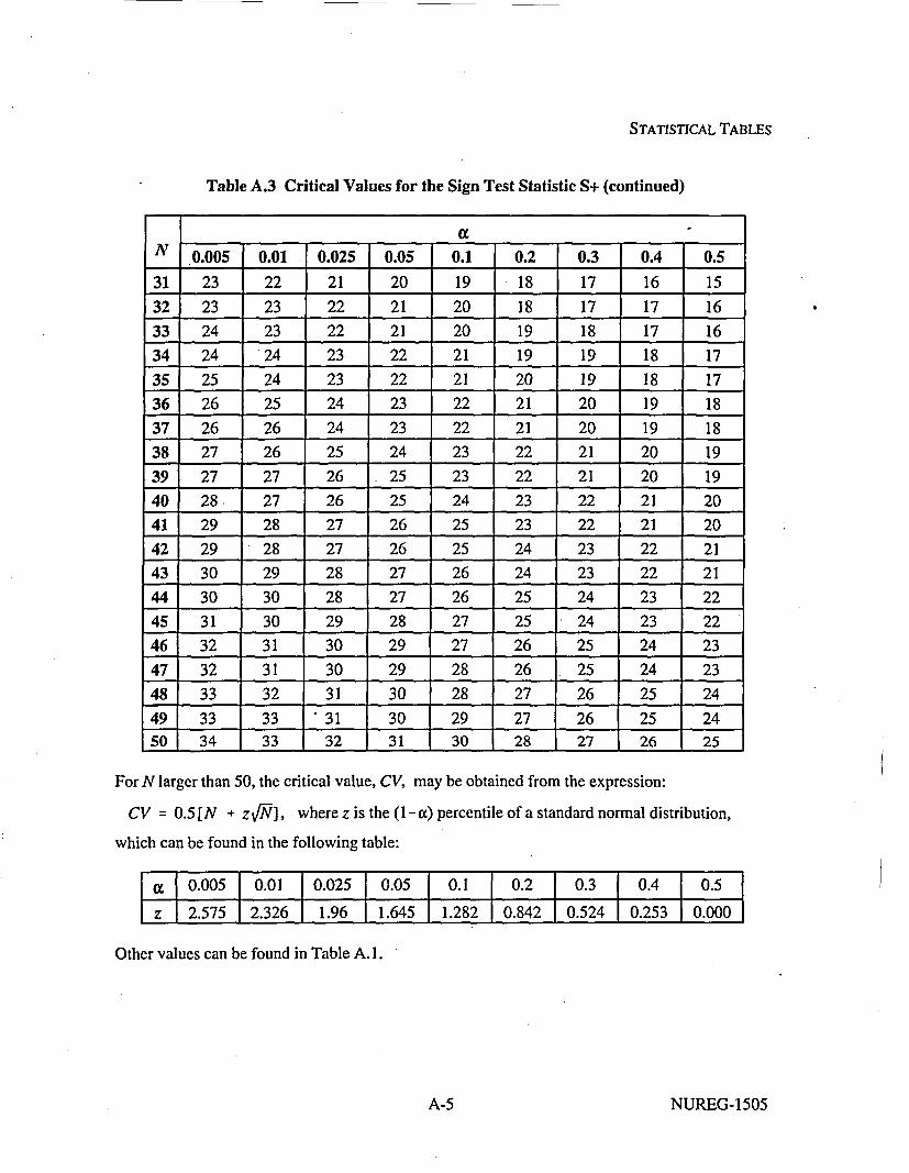
STATISTICAL TABLES
Table A.3 Critical Values for the Sign Test Statistic S+ (continued)
____ ___ _ __ __ ___ _ __ __ _ ___
N 0.005 0.01 0.025 0.05 0.1 0.2 0.3 0.4 0.5
31 23 22 21 20 19 18 17 16 15
32 23 23 22 21 20 18 17 17 16
33 24 23 22 21 20 19 18 17 16
34 24 *24 23 22 21 19 19 18 17
35 25 24 23 22 21 20 19 18 17
36 26 25 24 23 22 21 20 19 18
37 26 26 24 23 22 21 20 19 18
38 27 26 25 24 23 22 21 20 19
39 27 27 26 .25 23 22 21 20 19
40 28 27 26 25 24 23 22 21 20
41 29 28 27 26 25 23 22 21 20
42 29 28 27 26 25 24 23 22 21
43 30 29 28 27 26 24 23 22 21
44 30 30 28 27 26 25 24 23 22
45 31 30 29 28 27 25 24 23 22
46 32 31 30 29 27 26 25 24 23
47 32 31 30 29 28 26 25 24 23
48 33 32 31 30 28 27 26 25 24
49 33 33 31 30 29 27 26 25 2
50 34 33 32 31 30 28 27 26 2
For N larger than 50, the critical value, CV, may be obtained from the expression:
CV = 0.5 [N + zV FN], where z is the (1- a) percentile of a standard normal distribution,
which can be found in the following table:
IC 0I.005 0.01 I0.025 0.05 0.1 0.2 1 0.3 0.4 I0.51z 12.575 2.326 1.96 1.645 1.282 0.842 10.524 0.253 0.000
Other values can be found in Table A. 1.
A-5 A-S NUREG-1 505

STATISTICAL TABLES
Table A.4 Critical Values for the WRS Test
NOTE: When using this table under Scenario A, m is the number of reference area samples andn is the number of survey unit samples. When using this table for Scenario B, the roles of m andn in this table are reversed.
n= 2m=2 a-=0.001 7
a=0.005 7a--0.01 7a=0.025 7
N a--0.05 7a=-0.1 7
n= 2m=3 a-=0.001 12
a=0.005 12a=0.01 12a=0.025 12a=0.05 12a=0.1 11
n= 2rn=4 a--0.001 18
a=0.005 18t--0.0O 18
a=0.025 18a--0.05 18a--0.1 17
n= 2m=5 a--0.001 25
a--0.005 25a=0.01 25a--0.025 25a-=0.05 24a--0.1 23
n= 2m=6 a--0.001 33
a--0.005 33a-=0.01 33a--0.025 33a--0.05 32a--0.1 31
n= 2m=7 a=0.001 42
a--0.005 42a=0.01 42a=0.025 42a=0.05 41&--0.1 40
n= 2m= 8 a--0.001 52
a--0.005 52a=0.01 52a--0.025 51a=0.05 50a-=0.1 49
NUREG-1505
3999998
3151515151413
3222222222120
3303030292827
3393939373635
5131313131211
5212121201918
5303029282725
5403938373534
5514948474543
5636159575654
5757371696765
7171717171615
7272726252422
7383736343331
7504846444341
7635958565451
7757270686563
7898584817875
8191919181716
8303029272624
8424039373634
8545250484644
8676462605855
8817776737067
8959290868480
10232323222119
10363534323129
10494746444239
10636058565351
10777472696663
10928886838076
11252525232321
iII
393837353331
11535149474542
11676462605754
11827977737067
12272727252422
12424039373633
12575452504845
12726866636157
12888381787571
13 1429 3129 3128 3027 2926 2724 26
13 1445 4843 4642 4540 4238 4035 37
13 1460 6458 6156 5953 5651 5448 50
13 1476 8172 7770 7467 7164 6861 64
13 1493 9888 9386 9182 8779 8375 79
15333332312927
15514847454340
15686462595753
15858178757167
16353534333129
16545150474542
16716866625956
16898582797571
17373736343330
17565452504744
17757169666259
17948986827974
18393938363432
18595755525046
18787572696561
18989390868277
19414039383633
20434241403835
4
19 2062 6559 6258 6055 5752 5448 50
19 2082 8678 8176 7972 7568 7164 67
19 20102 10797 10194 9890 9486 8981 84
4454443424139
3 449 5649 55.48 5447 5246 5144 49
3 460 6860 6659 6557 6356 6254 60
6575453514947
6696665636158
6827977757370
9726967646259
9878381787572
15 16 17 18 19 20103 108 113 118 123 12898 103 107 112 117 12295 100 104 109 114 11891 95 100 104 109 11387 91 96 100 104 10883 87 91 94 98 102
11 12 13 14 15 16 17 18 19 2098 104 110 116 122 128 133 139 145 15194 99 105 110 116 121 127 132 138 14392 97 102 108 113 118 123 129 134 13988.93 98 103 108 113 118 123 128 13385 90 94 99 104 109 113 118 123 12881 85 90 94 99 103 108 112 117 121
11 12 13 14 15 16 17 18 19 209 10102 109 115 122 128 135 141 148 154 161 167 17498 104 110 116 122 129 135 141 147 153 159 16596 102 108 114 120 125 131 137 143 149 155 16192 98 104 109 115 121 126 132 137 143 149 15489 95 100 105 111 116 122 127 132 138 143 14885 91 96 101 106 111 116 121 126 131 136 141
. A-6
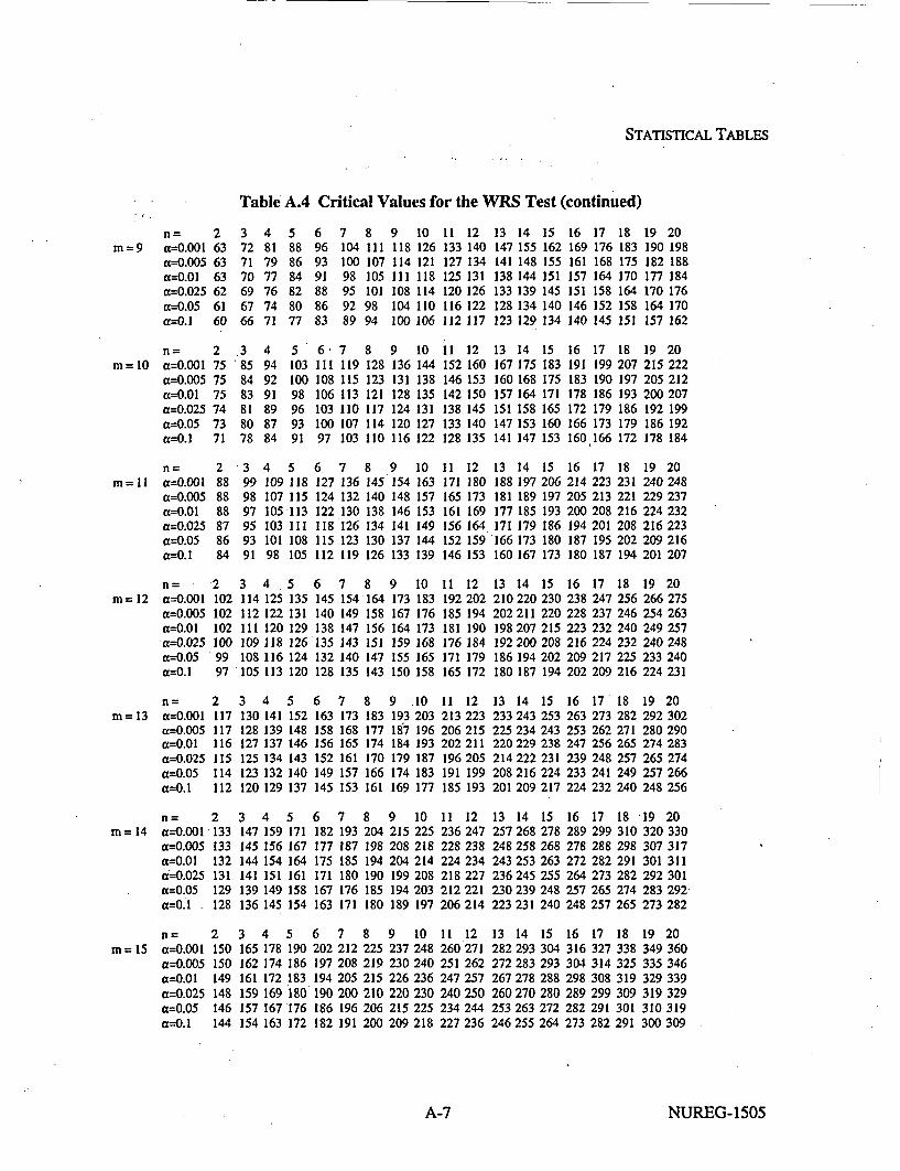
STATISTICAL TABLES
Table A.4 Critical Values for the WRS Test (continued)
n =
m=9 a--0.001a--0.005a=O.01a--0.025a--0.05a--O.!
2636363626160
3727170696766
.3'85
8483818078
4817977767471
4949291898784
5888684828077
510310098969391
6969391888683
7 8104 111100 10798 10595 10192 9889 94
9118114III108104100
m= 10 a--0.001a--0.005a--0.01a--0.025a=0.05a--0.1
nI=
m=11 a--0.001c--0.005a=0.01a=0.025a=0.05a--0. I
2757575747371
2888888878684
6"7 8 9111 119 128 136108 115 123 131106 113 121 128103 110 117 124100 107 114 12097 103 110 116
10126121118114110106
10144138135131127122
10163157153149144139
10183176173168165158
11133127125120116112
11
152146142138133128
11171165161156152146
12140134131126122117
12160153150145140135
12180173169164159153
13 14147 155141 148138 144133 139128 134123 129
15162155151145140134
16169161157151146140
16191183178172166160
13 14 15167 175 183160 168 175157 164 171151 158 165147 153 160141 147 153
17176168164158152145
18183175170164158151
17 18199 207190 197186 193179 186173 179166 172
19 20190 198182 188177 184170 176164 170157 162
19 20215 222205 212200 207192 199186 192178 184
3 4 5 6 7 8 999 109 118 127 136 145 15498 107 115 124 132 140 14897 105 113 122 130 138 14695 103 111 118 126 134 14193 101 108 115 123 130 13791 98 105 112 119 126 133
n = •2m = 12 a--0.001 102
a--0.005 102a--0.01 102a--0.025 100a--0.05 99a--O.l 97
3 4 5 6114 125 135 145112 122 131 140111 120 129 138109 118 126 135108 116 124 132105 113 120 128
7 8 9154164 173149 158 167147 156 164143 151 159140 147 155135 143 150
11 12192 202185 194181 190176 184171 179165 172
11 12213 223206215202 211196 205191 199185 193
13 14 15 16 17 18 19 20188 197 206 214 223 231 240 248181 189 197 205 213 221 229 237177 185 193 200 208 216 224 232171 179 186 194 201 208 216 223166 173 180 187 195 202 209 216160 167 173 180 187 194 201 207
13 14 15 16 17 18 19 20210 220 230 238 247 256 266 275202 211 220 228 237 246 254 263198 207 215 223 232 240 249 257192200208 216 224 232 240 248186 194 202 209 217 225 233 240180 187 194 202 209 216 224 231
13 14 15 16 17 18 19 20233 243 253 263 273 282 292 302225 234 243 253 262 271 280 290220 229 238 247 256 265 274 283214 222 231 239 248 257 265 274208 216 224 233 241 249 257 266201 209217 224 232 240 248 256
n--=
m = 13 a--0.001a--0.005ix=0.01a--0.025a=0.05a=0. I
2117117116115114112
3 4 5130 141 152128 139 148127 137 146125 134 143123 132 140120 129 137
3 4 5147 159 171145 156 167144 154 164141 151 161139 149 158136 145 154
6163158156152149145
7 8 9 .10173 183 193 203168 177 187 196165 174 184 193161 170 179 187157 166 174 183153 161 169 177
n= 2m= 14 a--0.001 133
a=0.005 133a--0.01 132d-=0.025 131a=0.05 129a--0.1 128
6 7 8 9 10 11 12 13 14 15 16 17 18 "19 20182 193 204 215 225 236 247 257 268 278 289 299 310 320 330177 187 198 208 218 228 238 248 258 268 278 288 298 307 317175 185 194 204 214 224 234 243 253 263 272 282 291 301 311171 180 190 199 208 218 227 236 245 255 264 273 282 292 301167 176 185 194 203 212 221 230 239 248 257 265 274 283 292163 171 180 189 197 206214 223 231 240 248 257 265 273 282
m= 15 a--0.001a--0.005a=0.01a--0.025a--0.05a--0. I
2 3 4 5150 165 178 190150 162 174 186149 161 172 183148 159 169 180146 157 167 176144 154 163 172
6 7202 212197 208194 205190 200186 196182 191
8 9 10 11 12225 237 248 260 271219 230 240 251 262215 226 236 247 257210 220 230 240 250206 215 225 234 244200 209 218 227 236
13 14 15282 293 304272 283 293267 278 288260 270 280253 263 272246 255 264
16 17316 327304 314298 308289 299282 291273 282
18338325319309301291
19 20349 360335 346329 339319 329310 319300 309
A-7 NUREG-1505

STATISTICAL TABLES
Table A.4 Critical Values for the WRS Test (continued)
m = 16 a--0.001a--0.005a=0.01a--0.025a--0.05a--O.
n--
m =17 a--0.001a--0.005a--0.01a--0.025a--0.05a---O.l
M =18 a--0.001a--0.005a--0.01a--0.025a=0.05a--O.l
m =19 a--0.001a--0.005a--0.01a--0.025a--0.05a---O.l
n =
rn=20 x--0.001a--0.005a--0.01a=0.025a--0.05ca-0.1
2168168167166164162
2187187186184183180
2207207206204202200
2228227226225223220
3 4 5 6 7 8 9 10184 197 210 223 236 248 260 272181 194 206 218 229 241 252 264180 192 203 215 226 237 248 259177 188 200 210 221 232 242 253175 185 196 206 217 227 237 247172 182 192 202 211 221 231 241
11 12284 296275 286270 281264 274257 267250 260
13 14 15 16 17 18 19 20308 320 332 343 355 367 379 390298 309 320 331 342 353 365 376292 303 314 325 336 347 357 368284 295 305 316 326 337 347 357278 288 298 308 318 328 338 348269 279 289 298 308 317 327 336
3 4 5 6 7 8 9 10 11 12203 218 232 245 258 271 284 297 310 322201 214 227 239 252 264 276 288 300312199 212 224 236 248 260 272 284 295 307197 209 220 232 243 254 266 277 288 299194 205 217 228 238 249 260 271 282 292191 202212 223 233 243 253 264 274 284
3 4 5 6 7 8 9 10 11 12224 239 254 268 282 296 309 323 336 349222 236 249 262 275 288 301 313 326 339220 233 246 259 272 284 296 309 321 333217 230 242 254 266 278 290 302 313 325215 226 238 250 261 273 284 295 307 318211 222 233 244 255 266 277 288 299 309
13 14 15335 347 360324 336 347318 330 341310321 332303 313 324294305 315
16 17 18 19 20372 384 397 409 422359 371 383 394 406353 364 376 387 399343 354 365 376 387335 345 356 366 377325 335 345 355 365
13 14 15 16 17 18 19 20362 376 389 402 415 428 441 454351 364 376 388 401 413 425 438345 357 370 382 394 406 418 430337 348 360 372 383 395 406418-329 340 352 363 374 385 396 407320 331 342 352 363 374 384 395
3 4 " 5246 262 277243 258 272242 256 269239 252 265236 248 261232 244 256
6 7 8 9 10 11 12292 307 321 335 350 364 377286 300 313 327 340 353 366283 296 309 322 335 348 361278 290 303 315 327 340 352273 285 297 309 321 333 345267 279 290 302 313 325 336
6 7 8 9 10 11 12317 333 348 363 377 392 407311 325 339 353 367 381 395307 321 335 349 362 376 389302 315 329 341 354 367 380297 310 322 335 347 360 372291 303 315 327 339 351 363
13 14 15391 405 419379 392 405373 386 399364377 389356 368 380347 358 370
13 14 15421 435 450409422 436402 416 429393 406 419385 397 409375 387 399
16 17 18 19 20433 446 460 473 487419 431 444 457 470411 424 437 449 462401 413 425 437 450392 403 415 427 439381 392 403 415 426
16 17 18 19 20464 479 493 507 521450 463 477 490 504442 456 469 482 495431 444 457 470 482422 434 446 459 471410 422 434 446 458
2 3 4 5250 269 286 302249 266 281 296248 264 279 293247 261 275 289245 258 271 284242 254 267 279
Reject the null hypothesis if the test statistic is greater than the table (critical) value.
For n or m greater than 20, the table (critical) value can be calculated for Scenario A from
m(n+m+l)12 + zlnm(n+m+1)ll2
if there are few or no ties, and from
m(n+m+l)/2 + z ]!i (n+m+l1)-E iI1) ]1j-l (n+m)(n+m-I)
if there are many ties, where g is the number of groups of tied measurements and tj is the numberof tied measurements in thejth group. For Scenario B, the roles of n and m are reversed in theseequations. z is the (1 -a) percentile of a standard normal distribution (see Table A. 1).
NUREG-1505 A-8

STATISTICAL TABLES
Table A.5a 0.025 and 0.975 Percentiles of the Chi-Squared Distribution
DOF 0.025 0.975 DOF 0.025 0.975 DOF 0.025 0.975 DOF 0.025 0.975____46 29.2 66.6 91 66.5 119.3 280 235.5 328.2
2 0.05 7.4 47 30 67.8 92 67.4 120.4 285 240.1 333.73 0.2 9.3 48 30.8 69.0 93 68.2 121.6 290 244.7 339.14 0.5 11.1 49 31.6 .70.2 94 69.1 122.7 295 249.3 344.55 0.8 12.8 50 32.4 71.4 95 69.9 123.9 300 253.9 349.96 1.2 14.4 51 33.2 72.6 96 70.8 125.0 305 258.5 355.37 1.7 16.0 52 34.0 73.8 97 71.6 126.1 310 263.1 360.78 2.2 17.5 53 34.8 75.0 98 72.5 127.3 315 267.7 366.19 2.7 19.0 54 35.6 76.2 99 73.4 128.4* 320 272.3 371.410 3.2 20.5 55 36.4 77.4 100 74.2 129.6 325 277.0 1376.811 3.8 21.9 56 37.2 78.6 105 78.5 135.2 330 281.6 382.212 4.4 23.3 57 38.0 79.8 110 82.9 140.9 335 286.2 387.613 5.0 24.7 58 38.8 80.9 115 87.2 146.6 340 290.8 393.014 5.6 26.1 59 39.7 82.1 120 91.6 152.2 345 295.4 398.415 6.3 27.5 60 40.5 83.3 125 95.9 157.8 350 300.1 403.716 6.9 28.8 61 41.3 84.5 130 100.3 163.5 355 304.7 409.117 7.6 30.2 62 42.1 85.7 135 104.7 169.1 360 309.3 414.518 8.2 31.5 63 43.0 86.8 140 109.1 174.6 365 314.0 419.819 8.9 32.9 64 43.8 88.0 145 113.6 180.2 370 318.6 425.220 9.6 34.2 65 44.6 89.2 150 118.0 185.8 375 323.2 430.521 10.3 35.5 66 45.4 90.3 155 122.4 191.4 380 327.9 435.922 11.0 36.8 67 46.3 91.5 160 126.9 196.9 385 332.5 441.323 11.7 38.1 68 47.1 92.7 165 131.3 202.5 390 337.2 446.624 12.4 39.4 69 47.9 93.9 170 135.8 208.0 395 341.8 452.025 13.1 40.6 70 48.8 95.0 175 140.3 213.5 400 346.5 457.326 13.8 41.9 71 49.6 96.2 180 144.7 219.0 405 351.1 462.727 14.6 43.2 72 50.4 97.4 185 149.2 224.6 410 355.8 468.028 15.3 44.5 73 51.3 98.5 190 153.7 230.1 415 360.5. 473.329 16.0 45.7 74 52.1 99.7 195 158.2 235.6 420 365.1 478.730 16.8 47.0 75 52.9 100.8 200 162.7 241.1 425 369.8 484.031 17.5 48.2 76 53.8 102.0 205 167.2 246.5 430 374.4 489.332 18.3 49.5 77 54.6 103.2 210 171.8 252.0 435 379.1 '494.733 19.0 50.7 78 55.5 104.3 215 176.3 257.5 440 383.8 500.034 19.8 52.0 79 56.3 105.5 220 180.8 263.0 445 388.4 505.335 20.6 53.2 80 57.2 106.6 225 185.3 268.4 450 393.1 510.736 21.3 54.4 81 58.0 107.8 230 189.9 273.9 455 397.8 516.037 22.1 55.7 82 58.8 108.9 235 194.4 279.4 460 402.5 521.3
'38 22.9 56.9 83 59.7 110.1 240 199.0 284.8 465 407.1 526.639 23.7 58.1 84 60.5 111.2 245 203.5 290.2 470 411.8 532.040 24.4 59.3 85 61.4 112.4 250 208.1 295.7 475 416.5 537.341 25.2 60.6 86 62.2 113.5 255 212.7 301.1 480 421.2 542.642 26.0 61.8 87 63.1 114.7 260 217.2 306.6 485 425.9 547.943 26.8 63.0 88 63.9 -115.8 265 221.8 312.0 490 430.6 553.244 27.6 64.2 89 64.8 117.0 270 226.4 317.4 495 435.2 558.545 28.4 .65.4 90 65.6 118.1 275 231.0 1322.8 500 _[43-9.9 1563.9
A-9 A-9 NUREG- 1505

STATISTIAL TABLES
Table A.5b 0.05 and 0.95 Percentiles of the Chi-Squared Distribution
DOF 0.05 0.95 DOF 0.05 0.95 DOF 0.05 0.95 DOF 0.05 0.95_______46 31.4 62.8 91 70.0 114.3 280 242.2 320.0
2 0.1 6.0 47 32.3 64.0 92 70.9 115.4 285 246.9 325.43 0.4 7.8 48 33.1 65.2 93 71.8 116.5 290 251.6 330.74 0.7 9.5 49 33.9 66.3 94 .72.6 ,117.6 295 256.2 336.15 1.1 11.1 50 34.8 67.5 95 73.5 118.8 300 260.9 341.46 1.6 12.6 51 35.6 68.7 96 74.4 119.9 3505 265.5 346.77 .2.2 14.1 52 36.4 69.8 97 75.3 121.0 310 270.2 352.18 2.7 15.5 53 37.3 71.0 98 76.2 122.1 315 274.9 357.49 3.3 16.9 54 38.1 72.2 99 77.0 123.2 320 279.6 362.710 3.9 18.3 55 39.0 73.3 100 77.9 124.3 325 284.2 368.011 4.6 19.7 56 39.8 74.5 105 82.4 129.9 330 288.9 373.412 5.2 21.0 57 40.6 75.6 110 86.8 135.5 335 293.6 378.713 5.9 22.4 58 41.5 76.8 115 91.2 141.0 340 298.3 384.014 6.6 23.7 59 42.3 77.9 120 95.7 146.6 345 303.0 389.315 7.3 25.0 60 43.2 79.1 125 100.2 152.1 350 307.6 394.616 8.0 26.3 61 44.0 80.2 130 104.7 157.6 355 312.3 399.917 8.7 27.6 62 44.9 81.4 135 109.2 163.1 360 317.0 405.218 9.4 28.9 63 45.7 82.5 140 113.7 168.6 365 321.7 410.519 10.1 30.1 64 46.6 83.7 145 118.2 174.1 370 326.4 415.920 10.9 31.4 65 47.4 84.8 150 122.7 179.6 375 331.1 421.221 11.6 32.7. 66 48.3 86.0 155 127.2 185.1 380 335.8 426.522 12.3 33.9 67 49.2 87.1 160 131.8 190.5 385 340.5 431.823 13.1 35.2 68 50.0 88.3 165 136.3 196.0 390 345.2 43724 13.8 36.4 69 50.9 89.4 170 140.8 201.4 395 349.9 442.325 14.6 37.7 70 51.7 90.5 175 145.4 206.9 400 354.6 447.626 15.4 38.9 71 52.6 91.7 180 150.0 212.3 405 359.4 452.927 16.2 40.1 72 53.5 92.8 185 154.5 217.7 410 364.1 458.228 16.9 41.3 73 54.3 93.9 190 159.1 223.2 415 368.8 463.529 17.7 42.6 74 55.2 95.1 195 163.7 228.6 420 373.5 468.830 18.5 43.8 75 56.1 96.2 200 168.3 234.0 425 378.2 474.131 19.3 45.0 76 56.9 97.4 205 172.9 239.4 430 382.9 479.332 20.1 46.2 77 57.8 98.5 210 177.5 244.8 435 387.6 484.633 20.9 47.4 78 58.7 99.6 215 182.1 250.2 440 392.4 489.934 21.7 48.6 79 59.5 100.7 220 186.7 255.6 445 397.1 495.235 22.5 49.8 80 60.4 101.9 225 191.3 261.0 450 401.8 500.536 23.3 51.0 81 61.3 103.0 230 195.9 266.4 455 406.5 505.737 24.1 52.2 82 62.1 104.1 235 200.5 271.8 460 411.3 511.038 24.9 53.4 83 63.0 105.3 240 205.1 277.1 465 416.0 516.339 25.7 54.6 84 63.9 106.4 245 209.8 282.5 470 420.7 521.540 26.5 55.8 85 64.7 107.5 250 214.4 287.9 475 425.5 526.841 27.3 56.9 86 65.6 108.6 255 219.0 293.2 480 430.2 532.142 28.1 58.1 87 66.5 109.8 260 223.7 298.6 485 434.9 537.343 29.0 59.3 88 67.4 110.9 265 228.3 304.0 490 439.7 542.644 29.8 60.5 89 68.2 112.0 270 232.9 309.3 495 444.4 547.945 30.6 61.7 90 69.1 .113.1 275 237.6 314.7 500 449.1 53.
NUREG-1505A-1 A-10

STATISTICAL TABLES
Table A.6 1000 Random Numbers Uniformly Distributed Between Zero and One
0.382000 0.100681 0.596484 0.899106 0.884610 0.958464 0.014496 0.407422 0.863247 0.1385850.245033 0.045473 0.032380 0.164129 0.219611 0.017090 0.285043 0.343089 0.553636 0.3573720.371838 0.355602 0.910306 0.466018 0.426160 0.303903 0.975707 0.806665 0.991241 0.2562640.951689 0.053438 0.705039 0.816523 0.972503 0.466323 0.300211 0.750206 0.351482 0.7756580.074343 0.198431 0.064058 0.358348 0.487045 0.511216 0.373455 0.985900 0.040712 0.2307200.004975 0.926145 0.100314 0.256691 0.775689 0.679647 0.809107 0.724326 0.085055 0.1322670.756157 0.626514 0.173650 0.404798 0.552324 0.711509 0.555162 0.181158 0.970275 0.6869410.528794 0.796686 0.805658 0.262215 0.177953 0.866756 0.114841 0.059511 0.761559 0.7383950.986297 0.925596 0.903867 0.544969 0.500778 0.674978 0.489822 0.145787 0.037965 0.7962580.671560 0.731681 0.584521 0.152226 0.892178 0.377819 0.200476 0.205786 0.333964 0.325144
0.300211 10.802179 0.696097 0.271493 0.904050 0.039 125 0.709037 0.4537 19 0.5 16648 0.2565390.291299 0.802149 0.789026 0.675954 0.755333 0.948515 0.619404 0.722068 0.968047 0.3686030.850429 0.557054 0.873074 0.441053 0.217750 0.859035 0.280343 0.703299 0.707389 0.3758350.329691 0.085971 0.976867 0.285531 0.534318 0.407392 0.997711 0.894711 0.810816 0.9085970.574511 0.706076 0.401440 0.111026 0.897366 0.386334 0.095798 0.777642 0.783563 0.66573 1
0.656850 0.258461 0.765191 0.700308 0.858821. 0.002808 0.678610 0.928831 0.042482 0.51814310.912137 0.954314 0.594317 0.557665 0.968169 0.483016 0.255623 0.817896 0.496048 0.8506420.668111 0.926939 0.451765 0.168096 0.061953 0.005158 0.541093 0.617603 0.492904 0.5794550.601886 0.930052 0.533982 0.132054 0.082278 0.575915 0.829218 0.065676 0.270943 0.6996980.414197 0.365581 0.435072 0.330088 0.211097 0.740471 0.523453 0.896786 0.603412 0.5227820.589770 0.584918 0.497024 0.110508 0.593036 0.558916 0.774102 0.230811 0.731193 0.5867180.545518 0.807337 0.964293 0.095370 0.108554 0.712271 0.883114 0.189917 0.015961 0.1845450.580035 0.930620 0.162328 0.195105 0.677847 0.548387 0:'294565 0.540819 0.173223 0.1853080.852351 0.029842 0.250771 0.431745 0.544877 0.967467 0.724082 0.951018 0.570269 0.9406410.259865 0.863244 0.883755 0.820887 0.041871 0.898312 0.420820 0.128208 0.030122 0.204718
0.682028 0.921291 0.472304 0.478530 0.584979 0.362407 0.823328 0.310556 0.990448 0.7715690.729270 0.163274 0.808313 0.926084 0.232276 0.381664 0.090182 0.911985 0.852016 0.5731380.014222 0.693411 0.700644 0.888028 0.168981 0.886013 0.287088 0.231574 0.042299 0.9153720.167180 0.938932 0.121555 0.341258 0.095462 0.944060 0.511490 0.629475 0.835566 0.9743640.475723 0.151585 0.284555 0.801660 0.808496 0.695242 0.068636 0.081332 0.442824 0.264687,0.265145 0.810297 0.200934 0.454268 0.408216 0.935545 0.093844 0.174780 0.433546 0.1443220.075777 0.015259 0.719321 0.367351 0.660054 0.020234 0.878536 0.025666 0.302469 0. 1644340.459975 0.553606 0.958678 0.306223 0.213416 0.227607 0.721305 0.900418 0.075594 0.8337960.943815 0.252419 0.533128 0.203742 0.756645 0.594531 0.518601 0.151555 0.382244 0.7656480.496139 0.841884 0.155309 0.775964 0.892819 0.121097 0.654134 0.037446 0.531602 0.8428600.849757 0.541856 0.223121 0.718528 0.678793 0.766930 0.171300 0.724631 0.946379 0.5926080.350017 0.598224 0.965484 0.008179 0.506699 0.451033 0.838801 0.891781 0.949034 0.0344550.789300 0.643147 0.771020 0.685781 0.446150 0.951476 0.675222 0.487564 0.491775 0.4790800.046205 0.671194 0.576434 0.742393 0.432936 0.795495 0.906827 0.97 1435 0.095004 0.7323830.414594 0.229041 0.770135 0.990143 0.91 1405 0.571306 0.318003 0.405896 0.136082 0.5298320.397961 0.738731 0.101321 0.698172 0.835597 0.193823 0.644856 0.702261 0.835353 0.4103210.592151 0.337565 0.695029 0.942595' 0.436842 0.153020 0.178442 0.767235 0.944792 0.2637410.202582 0.846797 0.588214 0.673330 0.995331 0.281198 0.216346 0.887326 0.380352 0.0783410.868526 0.098819 0.345164 0.075137 0.136021 0.727836 0.548448 0.040132 0.979186 0.5949580.923246 0.489242 0.405713 0.511582 '0.032014 0.245125 0.916623 0.566973 0.330088 0.2725910.125889 0.894131 0935 0.820124 0.460524 0.19516 0.466231 0.399457 0 .346446 0.8080390.388287 10.634632 0.787317 0.595080 0.051607 0.510758 0.742241 10.4355301 0.049532 10.055055
0..Q208197.1 0.602466 10.270211 10,9804389 0.41-4136 1 .065 082422 0.323283 10.032533 1 .860
A-11 A-li NUREG- 1505

STATISTICAL TABLES
Table A.6 1000 Random Numbers Uniformly Distributed Between Zero and One (continued)
0.539445 0.606800 0.814722 0.019013 0.247505 0.560747 0.556291 0.470656 0.404859 0.9291670.798975 0.091525 0.317698 0.397290 0.174932 0.421186 0.559557 0.168889 0.800104 0.4308600.759972 0.225105 0.622150 0.103946 0.988800 0.796197 0.130375 0.932188 0.392621 0.0776090.332774 0.608875 0.239357 0.721244 0.406964 0.701254 0.027192 0.133396 0.931364 0.5820180.814356 0.110660 0.102451 0.402142 0.425642 0.845058 0.845119 0.385937 0.692495 0.8290660.220954 10.229682 0.382153 0.693106 0.042573 0.884823 10.972777 0.505203 0.098636 0.5073400.930357 0.565050 0.896664 0.854518 0.643971 0.223579 0.329630 0.909757 0.675314 0.7590260.172857 0.017762 0.479110 0.840846 0.816828 0.310343 0.250435 0.612934 0.142796 0.7044890.055086 0.927061 0.947508 0.254158 0.899716 0.758171 0.822321 0.136662 0.897244 0.3322550.894345 0.055300 0.184576 0.998718 0.334727 0.338786 0.748619 0.377758 0.040986 0.5197610.816065 0.814844 0.399274 0.672750 0.964843 0.672597 0.533036 0.293008 0.611682 0.4921720.944273 0.998169 0.033418 0.554918 0.953581 0.832606 0.577563 0.875576 0.845332 0.4574720.218421 0.158483 0.124149 0.005921 0.1 15513 0.747948 0.788903 0.886196 0.329905 0.1038850.030519 0.312815 0.355022 0.834254 0.260231 0.847896 0.618427 0.815149 0.873440 0.7331770.610187 0.430342 0.656911 0.294473 0.794671 0.460952 0.244270 0.199683 0.961852 0.6569410.526933 0.851344 0.173956 0.521256 0.426038 0.695456 0.964629 0.338450 0.932218 0.7274390.945738 0.978454 0.819025 0.976653 0.478957 0.506973 0.936644 0.250526 0.568072 0.1339760.491592 0.920164 0.628040 0.531144 0.219459 0.027345 0.287332 0.049684 0.856014 0.4962310.879940 0.870052 0.813654 0.728660 0.782586 0.614124 0.469192 0.366253 0.254555 0.4520710.969054 0.499466 0.935179 0.234046 0.958464 0.105197 0.655873 0.678976 0.140599 0.9942320.723197 0.150853 0.072329 0.049440 0.328562 0.054598 0.101932 0.036836 0.241157 0.3819090.856441 0.769402 0.440474 0.438948 0.183264 0.906125 0.844386 0.286966 0.954039 0.1670580.789361 0.926969 0.634968 0.245521 0.418592 0.759667 0.032044 0.198798 0.635029 0.3524280.115635 0.598682 0.774468 0.043733 0.331706 0.222968 0.656362 0.417005 0.305551 0.5693230.167089 0.174657 0.344340 0.972533 0.033326 0.444044 0.644856 0.606586 0.940641 0.0459300.612262 0.152745 0.654134 0.757500 0.196844 0.415021 0.297617 0.100406 0.654347 0.6638690.446913 0.685781 0.636311 0.989959 0.193823 0.646870 0.017029 0.448683 0.837245 0.1908320.362743 0.277322 0.357433 0.801294 0.449965 0.965270 0.329722 0.121860 0.738639 0.4592120.433882 0.053316 0.206793 0.284555 0.215369 0.094302 0.452803 0.863735 0.255135 0.4577170.471084 0.813227 0.403394 0.993774 0.008576 0.500290 0.234413 0.450667 0.906888 0.6409500.378277 0.104862 0.337260 0.219703 0.885647 0.291208 0 .334605 0.513443 0.282022 0.865230,0.536180 0.499435 0.467940 0.127750 0.531877 0.429914 0.120792 0.244270 0.732139 0.8536030.755211 0.689261 0.159276 0.865780 0.097385 0.747276 0.069582 0.868282 0.930692 0.6019170.811060 0.620289 0.067843 0.044069 0.824061 0.861599 0.606433 0.330332 0.190893 0.2891930.123814 0.223182 0.640248 0.168859 0.967864 0.744072. 0.412915 0.362438 0.299387 0.6705530.895444 0.052797 0.043214 0.308939 0.427168 0.946837 10.403211 0.573534 0.187719 0.2386240.098300 0.903592 0.570605 0.113498 0.975494 0.049745 0.949370 0.07422 1 0.155797 0.2606590.242744 0.870907 0.370037 0.901120 0.184881 0.315409 0.639912 0.033387 0.706595 0.7621390.961303 0.992523 0.334574 0.535844 0.145756 0.486953 0.014252 0.087832 0.476363 0.2559890.262673 0.162389 0.334208 0.814905 0.057863 0.753716 0.452040 0.319407 0.370617 0.1353190.951018 0.080447 0.745293 0.743187 0.816828 0.760552 0.835383 0.193213 0.971679 0.7830740.300851 0.215155 0.598010 0.985809 0.972686 0.783410 0.870754 0.049684 0.691305 0.2265690.753624 0.734336 0.725364 0.596881 0.016511 0.451338 0.176397 0.080142 0.129551 0.2067930.276589 0.728629 0.190497 0.444288 0.984863 0.296884 0.541551 0.819300 0.788263 0.4627220.231910 0.436689 0.114872 0.213904 0.982208 0.582293 0.264016 0.682455 0.807215 0.4798430.260292 0.207038 0.953032 0.104526 0.537889 0.905576 0.304727 0.584613 0.861049 0.3384080.921445 0.221931 0.387249 0.944273 0.854060 0.662954 0.279092 0.829157 0.902921 0.2514730.771294 0.190527 -0.470717 0.0941 19 0.099124 0.157109 0.167852 0.870144 0.194250 0.5262310.325571 0.916288 0.554521- 0.779473 0.073763 0.618763 0.193701 0.858242 0.139470 0.6427500.077822 0.480300 0.022187- 0.03 1037 0.953795 0.278542 0.702658 0.703482 0.976897 0.5433520.540727 0.387371 0.043519 10.849574 0.519364 0.511490 0.235298 0.349712 10.490188 10.0936610.280221 0.014191 0.577441 10.154180 0.438429 0.600330 0.396466 10.685476 10.7174601 0.630940
NUREG- 1505 A1A-12

STATISTICAL TABLES
Table A.7a Values of r and k for the Quantile Test When a Is Approximately 0.01 (
Number of Survey Unit Measurements, n
m 5 10 15 20 25 30 35 40 45 50 55 60 65 70 75 80 85 90 95 100
5 r,k 11,11 13,13 16,16 19,19 22,22 25,25 28,21 r,k
a 0.008 0.015 0.014 0.013 0.013 0.013 0.011 a
10 6,6 7,7 9,9 11,11 13,13 14,14 16,16 18,18 19,19 21,21 23,22 25,2f 26,2( 28,21 30,30
0.005 0.013 0.012 0.011 0.01 0.014 0.013 0.012 0.01 0.014 0.013 0.012 0.015 0.01 0.01
15 3,3 7,6 6,6 7,7 8,8 10,10 11,11 12,12 13,13 15,15 16,1( 17,1 18,11 19,1 21,2 22,2, 23,2 24,2, 26,2 27,20.009 0.007 0.008 0.011 0.014 0.00 0.011 0.013 0.014 0.01 0.01 0.01 0.01 0.01 0.010.01 0.01, 0.01.1 0.01 0.01
20 6,4 4,4 5,5 6,6 7,7 8,8 9,9 10,10 11,11 12,12 13,13 14,1, 15,1! 16,1( 17,17 18,1 19,11 19,19 20,20 21,20.005 0.008 0.009 0.01 0.011 0.011 0.011 0.011 0.011 0.011 0.011 0.01: 0.01 0.01, 0.01: 0.01: 0.01 0.01.1 0.01 0.01
25 4,3 7,5 4,4 5,5 6,6 7,7 8,8 9,9 9,9 10,10 11,11 12,1: 12,12 13,1 14,1z 15,1! 16,1 16,1( 17,17 18,10.009 0.012 0.015 0.013 0.011 0.01 0.009 0.009 0.01 0.012 0.011 0.01 0.01 0.01 0.01 : 0.01 0.01 0.01, 0.01, 0.01
30 4,3 3,3 4,4 5,5 6,6 6,6 7,7 8,8 8,8 9,9 10,1 10,1 11,11 1211 12,1: 13,12 14,1 14,1 15,1 15,10.006 0.012 0.009 0.007 0.006 0.012 0.01 0.008 0.013 0.011 0.00 0.01 0.011 0.01 0.01: 0.01 0.011 0.01. 0.01 0.01
35 2,2 3,3 4,4 4,4 5,5 6,6 6,6 7,7 7,7 8,8 9,9 9,9 10,1C 10,1( 11,11 11,1 12,1 13,1 13,1' -14,1
0.013 0.008 0.006 0.014 0.01 0.007 0.012 0.009 0.014 0.011 0.00c. 0.01 0.01 0.01' 0.01 0.01 0.01, 0.01 0.01 0.01
40 2,2 3,3 7,5 4,4 5,5 5,5 6,6 6,6 7,7 7,7 8,8 8,8 9,9 9,9 10,1 10,1 11,11 11,11 12,1: 12,1"0.01 0.006 0.013 0.01 0.006 0.012 0.008 0.013 0.00ý 0.013 0.01 0.014 0.011 0.014 0.011 0.01, 0.01, 0.011 0.01: 0.01
45 2,2 6,4 3,3 4,4 4,4 5,5 5,5 6,6 6,6 7,7 7,7 8,8 8,8 9,9 9,9 10,1 10,1 10,1 11,1 11,I0.008 0.008 0.013 0.007 0.014 0.008 0.014 0.009 0.013 0.009 0.01 0.00S 0.01 0.00 0.01, 0.00W 0.01: 0.011 0.01 0.01
50 4,3 3,3 4,4 4,4 5,5 5,5 5,5 6,6 6,6 7,7 7,7 8,8 8,8 8,8 9,9 9,9 10,1 10,1 10,1
0.013 0.01 0.005 0.01 0.006 0.01 0.015 0.009 0.013 0.00 0.01 0.00 0.01 0.01 0.01 0.01! 0.01 0.013 0.01
55 4,3 3,3 7,5 4,4 4,4 5,5 5,5 6,6 6,6 6,6 7,7 7,7 8,8 8,8 8,8 9,9 9,9 9,9 10,10.01 0.008 0.013 0.008 0.014 0.007 0.011 0.007 0.01 0.01 0.00 0.01: 0.00E 0.01 0.012 0.00 0.01" 0.01' 0.01
60 4,3 3,3 3,3 4,4 4,4 5,5 5,5 5,5 6,6 6,6 6,6 7,7 7,7 7,7 8,8 8,8 8,8 9,9 9,90.0080.007 0.014 0.006 0.011 0.006 0.00 0.013 0.007 0.01 0.014 0.00. 0.01 0.01, 0.01 0.01: 0.01! 0.01 0.01ý
65 4,3 3,3 3,3 6,5 4,4 4,4 5,5 5,5 5,5 6,6 6,6 6,6 7,7 7,7 7,7 8,8 8,8 8,8 9,90.007 0.006 0.012 0.006 0.009 0.013 0.007 0.01 0.014 0.00 0.011 0.014 0.00S, 0.01 0.01 0.00 0.01, 0.01 0.01
70 2,2 6,4 3,3 7,5 4,4 4,4 5,5 5,5 5,5 5,5 6,6 6,6 6,6 7,7 7,7 7,7 8,8 8,8 8,80.014 0.008 0.01 0.013 0.007 0.011 0.005 0.008 0.011 0.01! 0.00E 0.011 0.01 0.00S 0.01 0.01 0.00,. 0.01 0.01.
75 2,2 4,3 3,3 3,3 4,4 4,4 4,4 5,5 5,5 5,5 6,6 6,6 6,6 6,6 7,7 7,7 7,7 8,8. 8,80.013 0.014 0.008 0.014 0.006 0.00 0.013 0.00 0.009 0.012 0.00 0.00S 0.01 0.01 0.00 0.01 0.01 0.00 0.0
80 2,2 4,3 3,3 3,3 6,5 4,4 4,4 5,5 5,5 5,5 5,5 6,6 6,6 6,6 6,6 7,7 7,7 7,7 7,70.011 0.012 0.007 0.012 0.006 0.008 0.011 0.005 0.00ý 0.01 0.013 0.00 0.00S 0.01 0.01, 0.00 0.01 0.01, 0.01
85 2,2 4,3 3,3 3,3 7,5 4,4 4,4 4,4 5,5 5,5 5,5 5,5 6,6 6,6 6,6 6,6 7,7 7,7 7,70.01 0.01 0.006 0.011 0.013 0.006 0.009 0.013 0.00 0.00 0.011 0.01 0.00- 0.01 0.01' 0.014 0.00 0.01 0.01
90 4,3 3,3 3,3 3,3 4,4 4,4 4,4 5,5 5,5 5,5 5,5 5,5 6,6 6,6 6,6 6,6 7,7 7,70.009 0.005 0.009 0.014 0.005 0.00' 0.011 0.005 0.00 0.00€. 0.01 0.01 0.00 0.01 0.01 0.01, 0.00 0.01
95 4,3 6,4 3,3 3,3 6,5 4,4 4,4 4,4 5,5 5,5 5,5 5,5 6,6 6,6 6,6 6,6 6,6 7,70.008 0.008 0.008 0.013 0.005 0.007 0.01 0.013 0.006 0.00a 0.01 0.01" 0.00j 0.001 0.01 0.011 0.01' 0.00
100 rk 4,3 4,3 3,3 3,3 7,5 4,4 4,4 4,4 4,4 5,5 5,5 5,5 5,5 6,6 6,6 6,6 6,6 6,6___ a 0.007 0.014 0.007 0.011 0.01 0.006 0.00 0.011 0.01 0.00 0.00 0.010.01 0.00 0.00 0.01 0.01 0.01
") Values of the parametersr and k needed for the Quantile test calculated by Gilbert and Simpson (PNL-7409,1992) for certain combinations of m (the number of measurements in the reference area) and n (the number ofmeasurements in the survey unit) The value of a listed is that obtained from simulation studies.
A-13 NUREG-1505

STATISTICAL TABLES
Table A.7b Values of r and k for the Quantile Test When a Is Approximately 0.025
Number of Survey Unit Measurements, nm 5 10 15 20 25 30 35 40 45 50 55 60 65 70 75 80 85 90 95 100
5 rk 9,9 12,12 15,15 17,17 20,20 22,22 25,25 r,k
0.03 0.024 0.021 0.026 0.024 0.028 0.025
10 7,6 6,6 8,8 9,9 11,11 12,12 14,1 17,17 18,18 20,2( 21,21 23,22 24,2ý 26,2( 27,27
0.029 0.028 0.022 0.029 0.024 0.029 0.02! 0.025 0.029 0.02f 0.02S 0.02( 0.02! 0.02( 0.02!
15 11,5 6,5 5,5 6,6 7,7 8,8 9,9 10,1 11,11 13,13 15,15 14,11 16,1( 17,1", 18,11 19,1! 21,2 21,2 22,2 23,20.03 0.023 0.021 0.024 0.026 0.02 0.028 0.02 0.03 0.02; 0.02 0.021 0.024 0.021 0.02! 0.020 0.02 0.02 0.02 0.02
20 8,4 3,3 4,4 5,5 6,6 7,7 12,11 13,11 9,9 10,1 11,11 12,1- 13,1. 13,11 14,11 15,1 16 1 17,1 17,17 18,10.023 0.03 0.026 0.024 0.022 0.02 0.021 0.02 0.028 0.02f 0.02, 0.02. 0.02: 0.02 0.02' 0.026 0.02 0.02, 0.02 0.0
25 2,2 8,5 6,5 7,6 5,5 6,6 10,9 7,7 8,8 13,12 9,9 10,1 11,1 11,1 12,1, 13,1 13,1. 14,1- 15,1 15,10.023 0.027 0.021 6.023 0.025 0.02 0.026 0.027 0.023 0.027 0.027 0.024 0.02: 0.021 0.02! 0.82 0.624 0.02 0.02 0.01
30 6,3 6,4 9,6 4,4 7,6 5,5 9,8 6,6 7,7 12,11 8,8 9,9 9,9 10,1( 10,1( 11,1 11,1 12,1 13,1 13,10.026 0.026 0.026 0.021 0.029 0.02J 0.024 0.029, 0.021 0.021 0.025 0.021 0.021 0.02: 0.02! 0.02! 0.03 0.02 2 0.0
35 7,3 4,3 3,3 6,5 4,4 10,8 5,5 9,8 6,6 7,7 7,7 8,8 8,8 9,9 9,9 10,1C 10,1 11,1 11,11 12,1
0.03 0.03 0.023 0.02 0.026 0.02 0.027 0.024 0.027 0.02 0.02" 0.021 0.024 0.021 0.02" 0.02 0.027 0.02 0.027 0.02
40 3,2 4,3 8,5 11,7 6,5 4,4 10,8 5,5 9,8 6,6 10,9 7,7 12,1 8,8 8,8 9,9 9,9 10,1 10,1 I1,10.029 0.022 0.028 0.025 0.028 0.03 0.026 0.027 0.023 0.02f 0.02E 0.024 0.02 0.02 0.02( 0.02 0.02 0.02 0.02 0.02
45 3,2 8,4 6,4 3,3 8,6 4,4 7,6 5,5 5,5 9,8 6,6 10,9 7,7 7,7 8,8 8,8 8,8 9,9 9,9 10,10.023 0.029 0.036 0.020 0.021 0.023 0.025 0.02 0.024 0.023 0.024 0.02 0.02: 0.02' 0.02 0.02 0.03 0.02 0.02 0.0
50 2,2 6,4 3,3 11,7 6,5 4,4 7,6 5,5 5,5 9,8 6,6 6,6 7,7 7,7 12,1 8,8 8,8 13,1 9,90.025 0.022 0.021 0.077 6.02 0.026 0.028 0.021 0.02E 0.02A 0.02- 0.02S 0.02 0.02! 0.02 0.02: 0.024 0.02 0.02
55 2,2 4,3 8,5 3,3 8,6 4,4 4,4 10,8 5,5 5,5 9,8 6,6 6,6 10,9 7,7 7,7 12,11 8,8 8,80.022 0.029 0.028 0.028 0.021 0.02 0.029 0.021 0.022 0.02E 0.02 0.09A 0.02 0.02 0.02. 0.027 0.02 0.02 0.02
60 14,5 4,3 8,5 3,3 11,7 6,5 4,4 7,6 10,8 5,5 5,5 9,8 6,6 6,6 10,9 7,7 7,7 7,7 8,80.022 0.024 0.021 0.023 0.029 0.024 0.02A 0.02A 0.024 0.023 0.02S 0.02, 0.02, 0.02" 0.027 0.021 0.02 0.03 0.02
65 6,3 7,4 6,4 10,6 3,3 8,6 6,5 4,4 7,6 10,8 5,5 5,5 9,8 6,6 6,6 10,9 7,7 7,7 7,70.028 0.021 0.025 0.025 0.02 0.021 0.029 0.026 0.02( 0.02f 0.022 0.02S 0.02 0.02. 0.02( 0.02 0.024 0.024 0.0
70 6,3 2,2 6,4 8,5 3,3 13,8 6,5 4,4 4,4 7,6 10,8 5,5 5,5 9,8 6,6 6,6 6,6 10,9 7,70.024 0.029 0.021 0.028 0.025 0.026 0.023 0.022 0.024 0.02E 0.02 0.02, 0.02J 0.02 0.021 0.02! 0.024 0.03 0.02
75 11,4 2,2 4,3 8,5 3,3 9,6 8,6 6,5 4,4 7,6 7,6 10,8 5,5 5,5 9,8 6,6 6,6 6,6 10,9
0.022 0.026 0.028 0.022 0.022 0.02 0.021 0.02 0.024 0.023 0.03 0.02S 0.02ý 0.02S 0.02 0.02 0.02, 0.021 0.02
80 7,3 2,2 4,3 6,4 10,6 3,3 13,8 6,5 4,4 4,4 7,6 10,8 5,5 5,5 5,5 9,8 6,6 6,6 6,60.028 0.024 0.024 0.028 0.024 0.02 0.027 0.023 0.02 0.02C 0.024 0.02 0.07 0.02! 0.02S 0.02 0.02 0.02ý 0.02
85 3,2 2,2 4,3 6,4 8,5 3,3 9,6 8,6 6,5 4,4 4,4 7,6 10,8 5,5 5,5 5,5 9,8 6,6 6,60.029 0.021 0.021 0.023 0.028 0.023 0.03 0.02 0.026 0.02 0.02E 0.02 0.02 0.021 0.02! 0.02 0.02 0.02 0.02
90 5,3 11,5 9,5 8,5 3,3 3,3 13,8 6,5 6,5 4,4 4,4 7,6 10,8 5,5 5,5 5,5 9,8 9,8
__0.02 0.027 0.023 0.023 0.021 0.028 0.028 0.022 0.029 0.02• 0.02 0.02[ 0.02( 0.02: 0.02• 0.03 0.02, 0.02
95 10,4 2,2 4,3 6,4 10,6 3,3 11,7 8,6 6,5 4,4 4,4 7,6 7,6 10,8 5,5 5,5 5,5 9,8
__0.029 0.029 0.028 0.029 0.023 0.025 0.02( 0.02 0.025 0.02' 0.02( 0.024 0.02• 0.02' 0.02, 0.021 0.03 0.02
100 r~k 6,3 2,2 4,3 6,4 8,5 3,3 3,3 13,8 6,5 6,5 4,4 4,4 7,6 10,8 10,8 5,5 5,5 5,5
___ 0.029 0.027 0.025 0.025 0.028 0.022 0.02€ 0.02• 0.02• 0.021 0.02! 0.02• 0.02: 0.02' 0.021 0.02: 0.02e 0.0
NUREG-1505 A-14

STATISTICAL TABLES
Table A.7c Values of r and k for the Quantile Test When ca Is Approximately 0.05
Number of Survey Unit Measurements, nm 5 10 15 20 25 30 35 40 45 50 55 60 65 70 75 80 85 90 95 100
5 rk 8,8 10,10 13 13 15 15 17,17 19,19 21,21 r,k
a 0.051 0.057 0.043 0.048 0.051 0.054 0.05( a
10 4,4 5,5 14,12 8,8 9,9 10,10 12,12 13,13 14,14 15,15 17,1' 18,1E 19,1S 20,2( 21,2 23,2.0.043 0.057 0.045 0.046 0.052 0.058 0.046 0.05 0.054 0.057 0.04ý 0.052 0.05f 0.05, 0.05S 0.05i
15 2,2 3,3 4,4 5,5 6,6 7,7 8,8 9,9 9,9 10,10 11,11 12,1, 13,11 14,11 15,1f 16,11 16,1i 17,1' 18,11 19,10.053 0.052 0.05 0.048 0.046 0.045 0.052 0.043 0.06 0.057 0.055 0.05ý 0.05' 0.051 0.05 0.04c 0.054 0.05" 0.054 0.05
20 9,4 8,5 6,5 4,4 5,5 9,8 6,6 7,7 8,8 8,8 9,9 10,1 10,1( 11,11 12,1, 12,12 13,1 14,1' 14,1, 15,10.04 0.056 0.04 0.053 0.043 0.052 0.056 48 0.043 0.05 0.051 0.041 0.05' 0.052 0.04 0.05, 0.05 0.04! 0.05" 0.05
25 6,3 6,4 3,3 6,5 4,4 5,5 5,5 6,6 11,1 7,7 8,8 8,8 9,9 9,9 10,1( 11,1 11,11 11,1 12,1 12,10.04110.043 0.046 0.052 0.055 0.041 0.059 0.046 0.042 0.05 0.042 0.053 0.04f 0.05 0.0 0.041 0.05 0.05 0.05: 0.0
30 3,2 2,2 10,6 3,3 11,8 4,4 8,7 5,5 6,6 6,6 7,7 7,7 8,8 8,8 9,9 9,9 9,9 10,1( 10,19 11,10.047 0.058 0.052 0.058 0.045 0.05 0.044 0.054 0.04 0.053 0.041 0.05 0.042 0.051 0.04 0.05 0.05 0.04 0.05' 0.04
35 8,3 2,2 6,4 3,3 6,5 4,4 4,4 8,7 5,5 9,8 6,6 6,6 7,7 7,7 8,8 8,8 8,8 9,9 9,9 10,10.046 0.045 0.058 0.043 0.041 0.04 0.057 0.043 0.051 0.052 0.047 0.051 0.042 0.051 0.041 0.04 0.051 0.045 0.05: 0.04
40 4,2 5,3 4,3 10,6 3,3 6,5 4,4 4,4 8,7 5,5 9,8 6,6 6,6 11,1 7,7 7,7 8,8 8,8 8,8 9,90.055 0.048 0.057 0.059 0.053 0.048 0.043 0.058 0.042 0.048 0.047 0.042 0.051 0.04, 0.04! 0.05ý 0.04 0.04 0.0 0.04
45 4,2 9.4 2,2 8,5 3,3 8,6 6,5 4,4 4,4 8,7 5,5 5,5 9,8 6,6 6,6 11,1C 7,7 7,7 8,8 8,8
0.045 0.047 0.059 0.052 0.042 0.041 0.054 0.045 0.058 0.041 0.04( 0.05 0.05( 0.041 0.05 0.04( 0.041 0.05 0.04 0.04
50 6,3 2,2 6,4 12,7 3,3 8,6 6,5 4,4 4,4 8,7 5,5 5,5 9,8 6,6 6,6 6,6 7,7 7,7 7,70.051 0.05 0.051 0.05 0.049 0.04 0.059 0.047 0.059 0.041 0.04f 0.05z 0.05 0.04' 0.05 0.051 0.041 0.041 0.05
55 3,2 2,2 4,3 8,5 3,3 5,4 6,5 9,7 4,4 4,4 8,7 5,5 5,5 9,8 6,6 6,6 6,6 11,1 7,7
10.059 0.043 0.056&0.058 0.041 0.041 0.046 0.04 0.04 0.05 0.04 0.04. 0.052 0.04E 0.04 0.041 0.05ý 0.04 0.04
60 3,2 5,3 4,3 6,4 3,3 3,3 8,6 6,5 9,7 4,4 4,4 13,10 5,5 5,5 5,5 9,8 6,6 6,6 6,60.052 0.052 0.046 0.059 0.035 0.047 0.043 51 0.046 0.049 0.055 0.052 0.04 0.05 0.051 0.05, 0.04, 0.05 0.05
65 .3,2 5,3 2,2 6,4 10,6 3,3 3,3 6,5 6,5 4,4 4,4 4,4 13,19 5,5 5,5 5,5 9,8 6,6 6,60.045 0.043 0.053 0.048 0.05 0.04 0.052 0.041 0.055 0.042 0.05 0.06 0.05 0.041 0.04E 0.05! 0.05, 0.041 0.04
70 8,3 9,4 2,2 4,3 8,5 5,4 3,3 3,3 6,5 6,5 4,4 4,4 4,4 13,10 5,5 5,5 5,5 9,8 9,80.057 0.048 0.047 0.055 0.05 0.041 0.046 0.057 0.04 0.058 0.04 0.051 0.06 0.05q 0.04. 0.04" 0.05 0.04 0.05
75 8,3 6,3 2,2 4,3 6,4 10,6 3,3 3,3 8,6 6,5 9,7 4,4 4,4 5,5 13,1( 8,7 5,5 5,5 5,50.049 0.056 0.043 0.047 0.054 0.053 0.04 0.051 0.044 0.049 0.041 0.044 0.052 0.06 0.05 0.04. 0.04( 0.05 0.05
80 4,2 6,3 5,3 2,2 6,4 8,5 5,4 3,3 3,3 6,5 6,5 9,7 4,4 4,4 7,6 13,1C 87 5,5 5,5.0.059 0.048 0.053 0.055 0.046 0.055 0.041 0.04 0.055 0.041 0.05- 0.04. 0.04f 0.052 0.05 0.05 0.04 0.04 0.05
85 4,2 3,2 5,3 2,2 4,3 4,3 10,6 5,4 3,3 3,3 6,5 6,5 9,7 4,4 4,4 7,6 10,8 8,7 5,50.054 0.058 0.047 0.05 0.054 0.048 0.056 0.049 0.04 0.05 0.044 0.05f 0.04( 0.04( 0.05' 0.05 0.06 0.04 0.04
90 3,2 5,3 2,2 6,4 6,4 8,5 5,4 3,3 3,3 8,6 6,5 6,5 4,4 4,4 4,4 7,6 10,8 8,70.053 0.041 0.046 0.059 0.051 0.058 0.042 0.044 0.053 0.045 0.04 0.05E 0.04 0.04, 0.05ý 0.05! 0.06 0.04
95 3,2 9,4 2,2 2,2 4,3 8,5 10,6 5,4 3,3 3,3 6,5 6,5 9,7 4,4 4,4 4,4 7,6 10,0.048 0.048 0.042 0.056 0.059 0.05 0.058 0.048 0.048 0.056 0.041 0.05 0.04( 0.04d 0.04J 0.05, 0.59 0.05
100 r,k 3,2 6,3 5,3 2,2 4,3 6,4 10,6 5,4 3,3 3,3 3,3 6,5 6,5 9,7 4,4 4,4 4,4 7,6
0.044 0.057 0.054 0.052 0.053 0.05 0.04 0.04 0.04 0.05 0.05 0.05 0.04 0.04 0.04 0.05 0.05
A-15 NUREG-1505

STATISTICAL TABLES
Table A.7d Values of r and k for the Quantile Test When a Is Approximately 0.10
Number of Survey Unit Measurements, n
m 5 10 15 20 25 30 35 40 45 50 55 60. 65 70 75 80 85 90 95 100
5 rk 7,7 8,8 10,10 12,12 14,14 15,1 17,17 r,k
a 0.083 0.116 0.109 0.104 0.1 0.11 0.11 a10 3,3 4,4 5,5 6,6 7,7 8,8 9,9 10,1( 11,11 12,12 13,1 14,14 15,1f 16,1( 1712 18,1
0.105 0.108 0.109 0.109 0.109 0.109 0.10 0.10 0.10S 0.10S 0.10S 0.10S 0.10S 0.10S 0.10! 0.10(
15 9,4 10,6 3,3 4,4 5,5 5,5 6,6 7,7 7,7 8,8 9,9 9,9 10,10 11,1 11,11 12,1: 13,1" 13,1 14,1 15,10.098 0.106 0.112 0.093 0.081 0.11 0.102 0.092 0.11 0.10( 0.09 0.11 0.10! 0.101 0.11 0.11 0.1 0.11 0.11 0.1C
20 3,2 2,2 5,4 3,3 4,4 4,4 5,5 10,9 6,6 7,7 7,7 8,8 8,8 9,9 9,9 10,1C 10,1 11,11 11,1 12,10.091 0.103 0.093 0.115 0.085 0.119 0.093 0.084 0.09 0.083 0.10: 0.081 0.10 0.09: 0.10' 0.09 0.10 0.09 0.11 0.1
25 4,2 7,4 8,5 3,3 3,3 4,4 4,4 8,7 5,5 10,9 6,6 6,6 7,7 7,7 8,8 8,8 8,8 9,9 9,9 10,10.119 0.084 0.112 0.08 0.117 0.08 0.107 0.10E 0.101 0.08E 0.09 0.114 0.093 0.104 0.09 0.1 0.11' 0.1 0. fi1: 0.09
30 4,2. 5,3 2,2 14,8 3,3 3,3 9,7 4,4 8,7 5,5 5,5 6,6 6,6 6,6 7,7 7,7 7,7 8,8 8,8 8,80.089 0.089 0.106 0.111 0.088 0.11 0.116 0.1 0.093 0.08E 0.10( 0.08 0.09 0.11 0.08' 0.1 0.11: 0.09 0.10 0.11
35 5,2 3,2 2,2 6,4 5,4 3,3 3,3 9,7 4,4 4,4 8,7 5,5 5,5 6,6 6,6 6,6 6,6 7,7 7,7 7,70.109 0.119 0.086 0.12 0.091 0.093 0.12 0.11 0.094 0.114 0.10' 0.09 0.11 0.08 0.09z 0.10 0.12 0.09, 0.10 0.11
40 5,2 3,2 5,3 2,2 12,7 5,4 3,3 6,5 9,7 4,4 4,4 8,7 5,5 5,5 5,5 6,6 6,6 6,6 6,6 7,70.087 0.098 0.119 0.107 0.109 0.102 0.097 0.10C 0.10ý 0.09 0.10• 0.09- 0.08ý 0.09S 0.11, 0.08 0.09 0.10 0.11 0.0
45 6,2 3,2 5,3 2,2 6,4 7,5 5,4 3,3 6,5 9,7 4,4 4,4 4,4 8,7 5,5 5,5 5,5 6,6 6,6 6,60.103 0.082 0.094 0.091 0.115 0.086 0.112 0.1 0.101 0.101 0.08 0.10: 0.11, 0.10, 0.09 0.10: 0.115 0.08 0.09 0.1
50 7,3 9,4 7,4 2,2 10,6 5,4 3,3 3,3 6,5 9,7 4,4 4,4 4,4 8,7 5,5 5,5 5,5 5,5 6,60.083 0.115 0.097 0.108 0.112 0.09 0.084 0.103 0.102 0.10f 0.08' 0.09 0.11, 0.09S 0.08 0.95 0.10 0.11 0.08
55 4,2 3,2 5,3 2,2 6,4 14,8 5,4 3,3 3,3 6,5 9,7 4,4 4,4 4,4 4,4 8,7 5,5 5,5 5,50.109 0.114 0.114 0.095 0.112 0.111 0.098 0.088 0.104 0.103 0.10z 0.08: 0.091 0.10" 0.12 0.10 0.08 0.09 0.10
60 4,2 3,2 5,3 2,2 2,2 8,5 5,4 5,4 3,3 3,3 6,5 9,7 4,4 4,4 4,4 4,4 8,7 5,5 5,50.095 0.1 0.097 0.084 0.109 0.119 0.081 0.105 0.091 0.10( 0.10. 0.10: 0.08 0.09', 0.10' 0.11. 0.1 0.08 0.09
65 4,2 3,2 5,3 7,4 2,2 6,4 12,7 5,4 5,4 3,3 3,3 6,5 9,7 7,6 4,4 4,4 4,4 8,7 8,70.084 0.089 0.082 0.090 0.097 0.11 0.113 0.089 0.111 0.092 0.10 0.10A 0.10 0.08, 0.09 0.1 0.11 0.09, 0.10
70 5,2 7,3 9,4 5,3 2,2 2,2 8,5 7,5 5,4 3,3 3,3 3,3 6,5 9,7 7,6 4,4 4,4 4,4 4,40.115 0.101 0.106 0.112 0.088 0.109 0.114 0.081 0.09( 0.08! 0.09e 0.105 0.10 0.19 0.08, 0.081 0.09 0.10 0.11
75 5,2 7,3 3,2 5,3 7,4 2,2 2,2 10,6 5,4 5,4 3,3 3,3 3,3 6,5 9,7 7,6 4,4 4,4 4,4103 0.088 0.111 0.098 0.101 0.09 0.119 0.11 0.083 0.10 0.085 0.094 0.11 0.10! 0.1 0.081 0.086 0.09 0.10
80 5,2 4,2 3,2 5,3 7,4 2,2 2,2 8,5 14,8 5,4 5,4 3,3 3,3 3,3 6,5 6,5 9,7 4,4 4,40.093 0.116 0.101 0.086 0.086 0.09! 0.109 0.111 0.11 0.08 0.10j 0.081 0.09, 0.11 0.10 0.12 0.11 0.08 0.09
85 5,2 4,2 3,2 9,4 5,3 2,2 2,2 2,2 10,6 7,5 5,4 5,4 3,3 3,3 3,3 6,5 6,5 9,7 4,40.084 0.106 0.092 117 0.111 0.083 0.101 0.11 0.112 0.08 0.09A 0.11 0.09 0.10 0.11 0.10 0.11 0.11 0.08
90 4,2 3,2 3,2 5,3 7,4 2,2 2,2 8,5 12,7 5,4 5,4 3,3 3,3 3,3 3,3 6,5 6,5 9,70.097 0.085 0.119 0.099 0.095 0.09 3 0.109 0.108 0.11 4 0.08 2 0.09 0.08 0.09 0.10 0.11 .0.10 0.11 1 0.11
95 4,2 7,3 3,2 5,3 7,4 2,2 2,2 2,2 10,6 14,8 5,4 5,4 3,3 3,3 3,3 3,3 6,5 6,50.089 100 0.11 0.089 0.084 0.086 0.102 0.11) 0.08 0.11 0.08E 0.10 0.08 0.09 0.10" 0.111 0.106 0.11
100 rk 4,2 7,3 3,2 5,3 5,3 2,2 2,2 2,2 6,4 12,7 7,5 5,4 5,4 3,3 3,3 3,3 3,3 6,5- 02 I I 0.080 . 0.1 0.11 0.1
NUREG-1505 A-16

NRC FORM 335 U.S. NUCLEAR REGULATORY COMMISSION 1. REPORT NUMBER(2-89) (Assigned by NRC, Add Vol., Supp.. Rev.,NRCM 1102. and Addendum Numbers, it any.)3201.3202 BIBLIOGRAPHIC DATA SHEET
(See Instructions on the reverse)
2. TITLE AND SUBTITLE NUREG-1505 Rev. 1
A Nonparametric Statistical Methodology for the Design and Analysis of Final StatusDecommissioning Surveys 3. DATE REPORT PUBLISHED
Interim Report for Use and Comment MONTH YEAR
June 19984. FIN OR GRANT NUMBER
5. AUTHOR(S) 6. TYPE OF REPORT
C.V. Gogolak*, Environmental Measurements LaboratoryG.E. Powers, U.S. Nuclear Regulatory Commission TechnicalA.M. Huffert, U.S. Nuclear Regulatory Commission 7. PERIOD COVERED (Inclusive Dates)
9/1/95 to 4/30/988. PERFORMING ORGANIZATION - NAME AND ADDRESS (If NRC, provide Division, Office or Region, U.S. Nuclear Regulatory Commission, and mailing address: if contractor,
provide name and mailing address.)
*U.S. Department of Energy Division of Regulatory Applications
Environmental Measurements Laboratory Office of Nuclear Regulatory Research201 Varick Street, 5th Floor U.S. Nuclear Regulatory CommissionNew York, NY 10014 Washington, DC 20555-0001
9. SPONSORING ORGANIZATION - NAME AND ADDRESS (If NRC, type "Same as above' If contractor, provide NRC Division, Office or Region, U.S. Nuclear Regulatory Commission,and mailing address.)
Division of Regulatory ApplicationsOffice of Nuclear Regulatory ResearchU.S. Nuclear Regulatory CommissionWashington, DC 20555-0001
10. SUPPLEMENTARY NOTES
George E. Powers, NRC Project Manager11. ABSTRACT (200 words or less)
.This report describes a nonparametric statistical methodology for the design and analysis of final status decommissioningsurveys in support of the final rulemaking on Radiological Criteria for License Termination published by the Nuclear RegulatoryCommission in the Federal Register on July 21, 1997. The techniques described are expected to be applicable to a broadrange of circumstances, but do not preclude the use of alternative methods as particular situations may warrant.Nonparametric statistical methods for testing compliance with decommissioning criteria are provided both for the case in whichthe radionuclides of concern occur in background and also for the case in which they do not occur in background. The testsdescribed are the Sign test, the Wilcoxon Rank Sum test, and a Quantile test. These tests are performed in conjunction with anElevated Measurement Comparison to provide confidence that the radiological criteria specified for license termination aremet. The Data Quality Objectives process is used for the planning of final site surveys. This includes methods for determiningthe number of samples needed to obtain statistically valid comparisons with decommissioning criteria and the methods forconducting the statistical tests with the resulting sample data.
12. KEY WORDS/DESCRIPTORS (List words or phrases that will assist researchers in locating the report.) 13. AVAILABILITY STATEMENT
Statistics, Decommissioning, Survey(s), Quality Assurance, Optimization, Nonparametric Statistics, unlimitedSign test, Wilcoxon Rank Sum test, Quantile test, Elevated Measurement Comparison 14. SECURITY CLASSIFICATION
(This Page)
unclassified(This Report)
unclassified15. NUMBER OF PAGES
16. PRICE
NRC FORM 335 (2-89) This form was eledroni Ily produced by Elite Federal Forms. IM
patper
Federal Recycling Program

UNITED STATESNUCLEAR REGULATORY COMMISSION
WASHINGTON, DC 20555-0001
FIRST CLASS MAILPOSTAGE AND FEES PAID
USNRCPERMIT NO. G-67
OFFICIAL BUSINESSPENALTY FOR PRIVATE USE, $300