Statistical Science2005, Vol. 20, No. 4, 317–337DOI 10.1214/088342305000000412© Institute of Mathematical Statistics, 2005

A Selective Overview of NonparametricMethods in Financial EconometricsJianqing Fan

Abstract. This paper gives a brief overview of the nonparametric techniquesthat are useful for financial econometric problems. The problems include es-timation and inference for instantaneous returns and volatility functions oftime-homogeneous and time-dependent diffusion processes, and estimationof transition densities and state price densities. We first briefly describe theproblems and then outline the main techniques and main results. Some use-ful probabilistic aspects of diffusion processes are also briefly summarized tofacilitate our presentation and applications.

Key words and phrases:Asset pricing, diffusion, drift, GLR tests, simu-lations, state price density, time-inhomogeneous model, transition density,volatility.

1. INTRODUCTION

Technological innovation and trade globalizationhave brought us into a new era of financial markets.Over the last three decades, a large number of newfinancial products have been introduced to meet cus-tomers’ demands. An important milestone occurred in1973 when the world’s first options exchange openedin Chicago. That same year, Black and Scholes [23]published their famous paper on option pricing andMerton [90] launched the general equilibrium modelfor security pricing, two important landmarks for mod-ern asset pricing. Since then the derivative marketshave experienced extraordinary growth. Professionalsin finance now routinely use sophisticated statisticaltechniques and modern computational power in portfo-lio management, securities regulation, proprietary trad-ing, financial consulting and risk management.

Financial econometrics is an active field that inte-grates finance, economics, probability, statistics andapplied mathematics. This is exemplified by the booksby Campbell, Lo and MacKinlay [28], Gouriérouxand Jasiak [60] and Cochrane [36]. Financial activitiesgenerate many new problems, economics provides use-ful theoretical foundation and guidance, and quantita-

Jianqing Fan is Professor, Benheim Center of Financeand Department of Operations Research and FinancialEngineering, Princeton University, Princeton, NewJersey 08544, USA (e-mail: jqfan@princeton.edu).

tive methods such as statistics, probability and appliedmathematics are essential tools to solve the quantitativeproblems in finance. To name a few, complex finan-cial products pose new challenges on their valuationand risk management. Sophisticated stochastic mod-els have been introduced to capture the salient featuresof underlying economic variables and to price deriva-tives of securities. Statistical tools are used to identifyparameters of stochastic models, to simulate complexfinancial systems and to test economic theories via em-pirical financial data.

An important area of financial econometrics is studyof the expected returns and volatilities of the price dy-namics of stocks and bonds. Returns and volatilitiesare directly related to asset pricing, proprietary trad-ing, security regulation and portfolio management. Toachieve these objectives, the stochastic dynamics ofunderlying state variables should be correctly speci-fied. For example, option pricing theory allows oneto value stock or index options and hedge against therisks of option writers once a model for the dynamicsof underlying state variables is given. See, for exam-ple, the books on mathematical finance by Binghamand Kiesel [20], Steele [105] and Duffie [42]. Yet manyof the stochastic models in use are simple and conve-nient ones to facilitate mathematical derivations andstatistical inferences. They are not derived from anyeconomics theory and hence cannot be expected to fitall financial data. Thus, while the pricing theory gives

317

318 J. FAN

spectacularly beautiful formulas when the underlyingdynamics is correctly specified, it offers little guid-ance in choosing or validating a model. There is al-ways the danger that misspecification of a model leadsto erroneous valuation and hedging strategies. Hence,there are genuine needs for flexible stochastic model-ing. Nonparametric methods offer a unified and eleganttreatment for such a purpose.

Nonparametric approaches have recently been intro-duced to estimate return, volatility, transition densitiesand state price densities of stock prices and bond yields(interest rates). They are also useful for examining theextent to which the dynamics of stock prices and bondyields vary over time. They have immediate applica-tions to the valuation of bond price and stock optionsand management of market risks. They can also be em-ployed to test economic theory such as the capital assetpricing model and stochastic discount model [28] andanswer questions such as if the geometric Brownianmotion fits certain stock indices, whether the Cox–Ingersoll–Ross model fits yields of bonds, and if in-terest rate dynamics evolve with time. Furthermore,based on empirical data, one can also fit directly theobserved option prices with their associated character-istics such as strike price, the time to maturity, risk-freeinterest rate, dividend yield and see if the option pricesare consistent with the theoretical ones. Needless tosay, nonparametric techniques will play an increas-ingly important role in financial econometrics, thanksto the availability of modern computing power and thedevelopment of financial econometrics.

The paper is organized as follows. We first intro-duce in Section 2 some useful stochastic models formodeling stock prices and bond yields and then brieflyoutline some probabilistic aspects of the models. InSection 3 we review nonparametric techniques used forestimating the drift and diffusion functions, based oneither discretely or continuously observed data. In Sec-tion 4 we outline techniques for estimating state pricedensities and transition densities. Their applications inasset pricing and testing for parametric diffusion mod-els are also introduced. Section 5 makes some conclud-ing remarks.

2. STOCHASTIC DIFFUSION MODELS

Much of financial econometrics is concerned withasset pricing, portfolio choice and risk management.Stochastic diffusion models have been widely used fordescribing the dynamics of underlying economic vari-ables and asset prices. They form the basis of many

spectacularly beautiful formulas for pricing contingentclaims. For an introduction to financial derivatives, seeHull [78].

2.1 One-Factor Diffusion Models

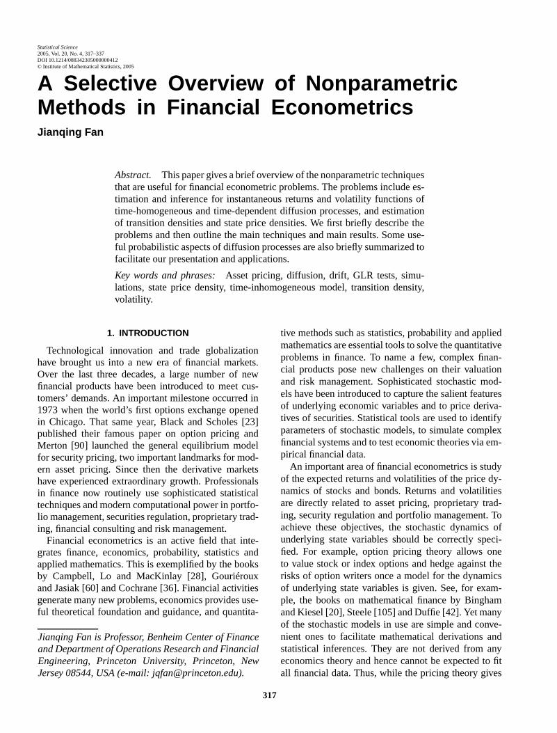
Let St� denote the stock price observed at timet�.The time unit can be hourly, daily, weekly, among oth-ers. Presented in Figure 1(a) are the daily log-returns,defined as

log(St�) − log(S(t−1)�

) ≈ (St� − S(t−1)�

)/S(t−1)�,

of the Standard and Poor’s 500 index, a value-weightedindex based on the prices of the 500 stocks that accountfor approximately 70% of the total U.S. equity (stock)market capitalization. The styled features of the returnsinclude that the volatility tends to cluster and that the(marginal) mean and variance of the returns tend to beconstant. One simplified model to capture the secondfeature is that

log(St�) − log(S(t−1)�

) ≈ µ0 + σ0εt ,

where{εt } is a sequence of independent normal randomvariables. This is basically a random walk hypothesis,regarding the stock price movement as an independentrandom walk. When the sampling time unit� getssmall, the above random walk can be regarded as arandom sample from the continuous-time process:

d log(St ) = µ0 + σ1 dWt,(1)

where {Wt } is a standard one-dimensional Brownianmotion andσ1 = σ0/

√�. The process (1) is called

geometric Brownian motion asSt is an exponent ofBrownian motionWt . It was used by Osborne [92]to model the stock price dynamic and by Black andScholes [23] to derive their celebrated option price for-mula.

Interest rates are fundamental to financial markets,consumer spending, corporate earnings, asset pricing,inflation and the economy. The bond market is evenbigger than the equity market. Presented in Figure 1(c)are the interest rates{rt } of the two-year U.S. Treasurynotes at a weekly frequency. As the interest rates gethigher, so do the volatilities. To appreciate this, Fig-ure 1(d) plots the pairs{(rt−1, rt − rt−1)}. Its dynamicis very different from that of the equity market. Theinterest rates should be nonnegative. They possess het-eroscedasticity in addition to the mean-revision prop-erty: As the interest rates rise above the mean levelα,there is a negative drift that pulls the rates down; whilewhen the interest rates fall belowα, there is a posi-tive force that drives the rates up. To capture these two

A SELECTIVE OVERVIEW 319

FIG. 1. (a)Daily log-returns of the Standard and Poor’s500 index from October 21, 1980 to July 29, 2004. (b) Scatterplot of the returnsagainst logarithm of the index( price level). (c) Interest rates of two-year U.S. Treasury notes from June 4, 1976 to March 7, 2003 sampledat weekly frequency. (d) Scatterplot of the difference of yields versus the yields.

main features, Cox, Ingersoll and Ross [37] derived thefollowing model for the interest rate dynamic:

drt = κ(α − rt ) dt + σr1/2t dWt .(2)

For simplicity, we will refer it to as the CIR model. Itis an amelioration of the Vasicek model [106],

drt = κ(α − rt ) dt + σ dWt,(3)

which ignores the heteroscedasticity and is also re-ferred to as the Ornstein–Uhlenbeck process. Whilethis is an unrealistic model for interest rates, theprocess is Gaussian with explicit transition density. Itfact, the time series sampled from (3) follows the au-toregressive model of order 1,

Yt = (1− ρ)α + ρYt−1 + εt ,(4)

where Yt = rt�, ε ∼ N(0, σ 2(1 − ρ2)/(2κ)) andρ = exp(−κ�). Hence, the process is well understood

and usually serves as a test case for proposed statisticalmethods.

There are many stochastic models that have been in-troduced to model the dynamics of stocks and bonds.Let Xt be an observed economic variable at timet .This can be the price of a stock or a stock index, orthe yield of a bond. A simple and frequently used sto-chastic model is

dXt = µ(Xt) dt + σ(Xt) dWt .(5)

The functionµ(·) is often called a drift or instanta-neous return function andσ(·) is referred to as a dif-fusion or volatility function, since

µ(Xt) = lim�→0

�−1E(Xt+� − Xt |Xt),

σ 2(Xt) = lim�→0

�−1 var(Xt+�|Xt).

320 J. FAN

The time-homogeneous model (5) contains many fa-mous one-factor models in financial econometrics. Inan effort to improve the flexibility of modeling interestdynamics, Chan et al. [29] extends the CIR model (2)to the CKLS model,

dXt = κ(α − Xt) dt + σXγt dWt .(6)

Aït-Sahalia [3] introduces a nonlinear mean rever-sion: while interest rates remain in the middle partof their domain, there is little mean reversion, and atthe end of the domain, a strong nonlinear mean re-version emerges. He imposes the nonlinear drift of theform (α0X

−1t + α1 + α2Xt + α2X

2t ). See also Ahn and

Gao [1], which models the interest rates byYt = X−1t ,

in which theXt follows the CIR model.Economic conditions vary over time. Thus, it is

reasonable to expect that the instantaneous returnand volatility depend on both time and price levelfor a given state variable such as stock prices andbond yields. This leads to a further generalization ofmodel (5) to allow the coefficients to depend on timet :

dXt = µ(Xt , t) dt + σ(Xt , t) dWt .(7)

Since only a trajectory of the process is observed[see Figure 1(c)], there is not sufficient informationto estimate the bivariate functions in (7) without fur-ther restrictions. [To consistently estimate the bivariatevolatility function σ(x, t), we need to have data thateventually fill up a neighborhood of the point(t, x).]A useful specification of model (7) is

dXt = {α0(t) + α1(t)Xt }dt + β0(t)Xβ1(t)t dWt .(8)

This is an extension of the CKLS model (6) byallowing the coefficients to depend on time and wasintroduced and studied by Fan et al. [48]. Model (8) in-cludes many commonly used time-varying models forthe yields of bonds, introduced by Ho and Lee [75],Hull and White [79], Black, Derman and Toy [21] andBlack and Karasinski [22], among others. The expe-rience in [48] and other studies of the varying coeffi-cient models [26, 31, 74, 76] shows that coefficientfunctions in (8) cannot be estimated reliably due tothe collinearity effect in local estimation: localizing inthe time domain, the process{Xt } is nearly constantand henceα0(t) andα1(t) andβ0(t) andβ1(t) cannoteasily be differentiated. This leads Fan et al. [48] tointroduce the semiparametric model

dXt = {α0(t) + α1Xt }dt + β0(t)Xβt dWt(9)

to avoid the collinearity.

2.2 Some Probabilistic Aspects

The question when there exists a solution to the sto-chastic differential equation (SDE) (7) arises naturally.Such a program was first carried out by Itô [80, 81].For SDE (7), there are two different meanings of solu-tion: strong solution and weak solution. See Sections5.2 and 5.3 of [84]. Basically, for a given initial con-dition ξ , a strong solution requires thatXt is deter-mined completely by the information up to timet . Un-der Lipschitz and linear growth conditions on the driftand diffusion functions, for everyξ that is independentof {Ws}, there exists a strong solution of equation (7).Such a solution is unique. See Theorem 2.9 of [84].

For the one-dimensional time-homogeneous diffu-sion process (5), weaker conditions can be obtained forthe so-called weak solution. By an application of theItô formula to an appropriate transform of the process,one can make the transformed process have zero drift.Thus, we can consider without loss of generality thatthe drift in (5) is zero. For such a model, Engelbertand Schmidt [45] give a necessary and sufficient condi-tion for the existence of the solution. The continuity ofσ suffices for the existence of the weak solution. SeeTheorem 5.5.4 of [84], page 333, and Theorem 23.1of [83].

We will use several times the Itô formula. For theprocessXt in (7), for a sufficiently regular functionf([84], page 153),

df (Xt , t) ={∂f (Xt , t)

∂t

+ 1

2

∂2f (Xt , t)

∂x2 σ 2(Xt , t)

}dt(10)

+ ∂f (Xt , t)

∂xdXt .

The formula can be understood as the second-orderTaylor expansion off (Xt+�, t + �) − f (Xt , t) bynoticing that(Xt+� − Xt)

2 is approximatelyσ 2(Xt ,

t)�.The Markovian property plays an important role

in statistical inference. According to Theorem 5.4.20of [84], the solutionXt to equation (5) is Markovian,provided that the coefficient functionsµ and σ arebounded on compact subsets. Letp�(y|x) be the tran-sition density, the conditional density ofXt+� = y

given Xt = x. The transition density must satisfy theforward and backward Kolmogorov equations ([84],page 282).

Under the linear growth and Lipschitz conditions,and additional conditions on the boundary behavior of

A SELECTIVE OVERVIEW 321

the functionsµ andσ , the solution to equation (1) ispositive and ergodic. The invariant density is given by

f (x) = 2C0σ−2(x)

(11)

·exp(−2

∫ x

.µ(y)σ−2(y) dy

),

whereC0 is a normalizing constant and the lower limitof the integral does not matter. If the initial distri-bution is taken from the invariant density, then theprocess{Xt } is stationary with the marginal densityfand transition densityp�.

Stationarity plays an important role in time seriesanalysis and forecasting [50]. The structural invariabil-ity allows us to forecast the future based on the his-torical data. For example, the structural relation (e.g.,the conditional distribution, conditional moments) be-tweenXt andXt+� remains the same over timet . Thismakes it possible to use historical data to estimate theinvariant quantities. Associated with stationarity is theconcept of mixing, which says that the data that are farapart in time are nearly independent. We now describethe conditions under which the solution to the SDE (1)is geometrically mixing.

Let Ht be the operator defined by

(Htg)(x) = E(g(Xt)|X0 = x

), x ∈ R,(12)

wheref is a Borel measurable bounded function onR.A stationary processXt is said to satisfy the conditionG2(s, α) of Rosenblatt [95] if there exists ans suchthat

‖Hs‖22 = sup

{f : Ef (X)=0}E(Hsf )2(X)

Ef 2(X)≤ α2 < 1,

namely, the operator is contractive. As a consequenceof the semigroup (Hs+t = HsHt ) and contraction prop-erties, the conditionG2 implies [16, 17] that for anyt ∈ [0,∞), ‖Ht‖2 ≤ αt/s−1. The latter implies, by theCauchy–Schwarz inequality, that

ρ(t) = supg1,g2

corr(g1(X0), g2(Xt)

) ≤ αt/s−1,(13)

that is, theρ-mixing coefficient decays exponentiallyfast. Banon and Nguyen [18] show further that fora stationary Markov process,ρ(t) → 0 is equivalentto (13), namely,ρ-mixing and geometricρ-mixing areequivalent.

2.3 Valuation of Contingent Claims

An important application of SDE is the pricing of fi-nancial derivatives such as options and bonds. It formsa beautiful modern asset pricing theory and providesuseful guidance in practice. Steele [105], Duffie [42]and Hull [78] offer very nice introductions to the field.

The simplest financial derivative is the European calloption. A call option is the right to buy an asset at acertain priceK (strike price) before or at expirationtime T . A put option gives the right to sell an assetat a certain priceK (strike price) before or at expira-tion. European options allow option holders to exerciseonly at maturity while American options can be exer-cised at any time before expiration. Most stock optionsare American, while options on stock indices are Euro-pean.

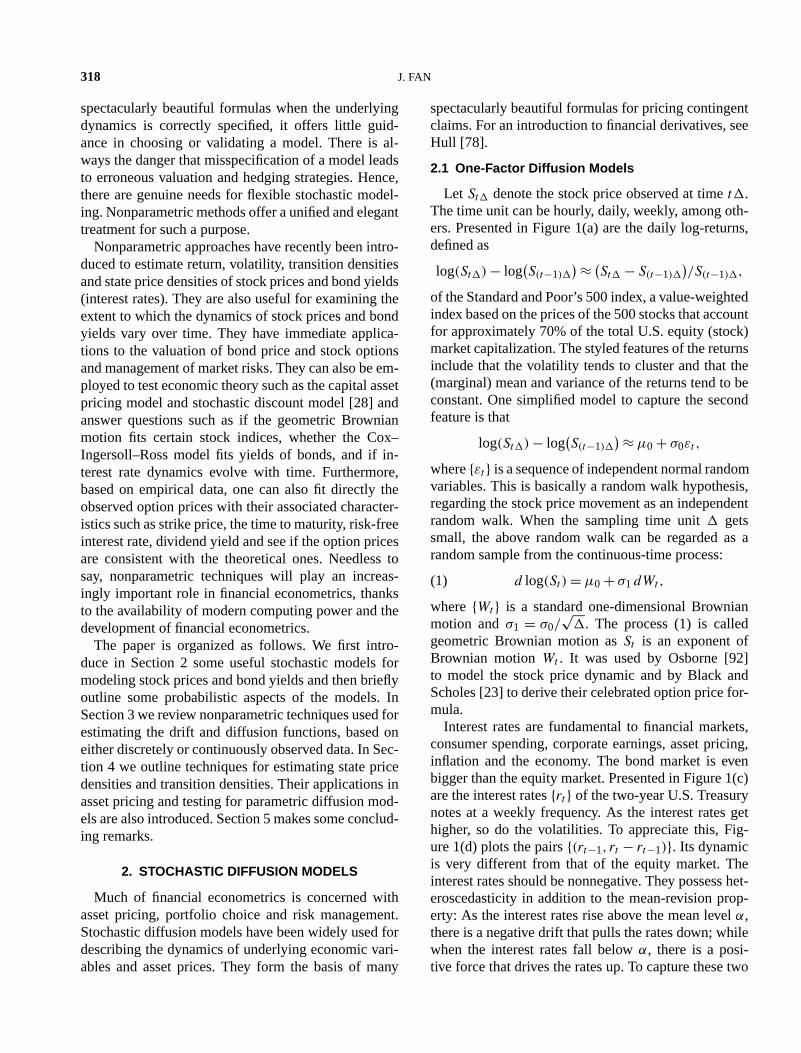
The payoff for a European call option is(XT −K)+,whereXT is the price of the stock at expirationT .When the stock rises above the strike priceK , one canexercise the right and make a profit ofXT − K . How-ever, when the stock falls belowK , one renders one’sright and makes no profit. Similarly, a European put op-tion has payoff(K − XT )+. See Figure 2. By creatinga portfolio with different maturities and different strikeprices, one can obtain all kinds of payoff functions. Asan example, suppose that a portfolio of options con-sists of contracts of the S&P 500 index maturing in sixmonths: one call option with strike price $1,200, oneput option with strike price $1,050 and $40 cash, butwith short position (borrowing or−1 contract) on a calloption with strike price $1,150 and on a put option withstrike price $1,100. Figure 2(c) shows the payoff func-tion of such a portfolio of options at the expirationT .Clearly, such an investor bets the S&P 500 index willbe around $1,125 in six months and limits the risk ex-posure on the investment (losing at most $10 if his/herbet is wrong). Thus, the European call and put optionsare fundamental options as far as the payoff functionat time T is concerned. There are many other exoticoptions such as Asian options, look-back options andbarrier options, which have different payoff functions,and the payoffs can be path dependent. See Chapter 18of [78].

Suppose that the asset price follows the SDE (7) andthere is a riskless investment alternative such as a bondwhich earns compounding rate of interestrt . Supposethat the underlying asset pays no dividend. Letβt bethe value of the riskless bond at timet . Then, with aninitial investmentβ0,

βt = β0 exp(∫ t

0rs ds

),

322 J. FAN

FIG. 2. (a)Payoff of a call option. (b)Payoff of a put option. (c)Payoff of a portfolio of four options with different strike prices and different(long and short) positions.

thanks to the compounding of interest. Suppose thata probability measureQ is equivalent to the originalprobability measureP , namelyP(A) = 0 if and only ifQ(A) = 0. The measureQ is called an equivalent mar-tingale measure for deflated price processes of givensecurities if these processes are martingales with re-spect toQ. An equivalent martingale measure is alsoreferred to as a “risk-neutral” measure if the deflater isthe bond price process. See Chapter 6 of [42].

When the markets are dynamically complete, theprice of the European option with payoff�(XT ) withinitial priceX0 = x0 is

P0 = exp(−

∫ T

0rs ds

)EQ(

�(XT )|X0 = x0),(14)

whereQ is the equivalent martingale measure for thedeflated price processXt/βt . Namely, it is the dis-counted value of the expected payoff in the risk neutralworld. The formula is derived by using the so-calledrelative pricing approach, which values the price of theoption from given prices of a portfolio consisting of arisk-free bond and a stock with the identical payoff asthe option at the expiration.

As an illustrative example, suppose that the price ofa stock follows the geometric Brownian motiondXt =µXt dt + σXt dWt and that the risk-free rater is con-stant. Then the deflated price processYt = exp(−rt)Xt

follows the SDE

dYt = (µ − r)Yt dt + σYt dWt .

The deflated price process is not a martingale as thedrift is not zero. The risk-neutral measure is the one

that makes the drift zero. To achieve this, we ap-peal to the Girsanov theorem, which changes the driftof a diffusion process without altering the diffusionvia a change of probability measure. Under the “risk-neutral” probability measureQ, the processYt satisfiesdYt = σYt dWt , a martingale. Hence, the price processXt = exp(rt)Yt underQ follows

dXt = rXt dt + σXt dWt .(15)

Using exactly the same derivation, one can easily gen-eralize the result to the price process (5). Under therisk-neutral measure, the price process (5) follows

dXt = rXt dt + σ(Xt) dWt .(16)

The intuitive explanation of this is clear: all stocks un-der the “risk-neutral” world are expected to earn thesame rate as the risk-free bond.

For the geometric Brownian motion, by an applica-tion of the Itô formula (10) to (15), we have under the“risk-neutral” measure

logXt − logX0 = (r − σ 2/2)t + σ 2Wt.(17)

Note that given the initial priceX0, the price fol-lows a log-normal distribution. Evaluating the expec-tation of (14) for the European call option with payoff�(XT ) = (XT − K)+, one obtains the Black–Scholes[23] option pricing formula

P0 = x0�(d1) − K exp(−rT )�(d2),(18)

whered1 = {log(x0/K)+ (r +σ 2/2)T }{σ√T }−1 and

d2 = d1 − σ√

T .

A SELECTIVE OVERVIEW 323

2.4 Simulation of Stochastic Models

Simulation methods provide useful tools for thevaluation of financial derivatives and other financialinstruments when the analytical formula (14) is hardto obtain. For example, if the price under the “risk-neutral” measure is (16), the analytical formula forpricing derivatives is usually not analytically tractableand simulation methods offer viable alternatives (to-gether with variance reduction techniques) to evaluateit. They also provide useful tools for assessing perfor-mance of statistical methods and statistical inferences.

The simplest method is perhaps the Euler scheme.The SDE (7) is approximated as

Xt+� = Xt + µ(t,Xt)� + σ(t,Xt)�1/2εt ,(19)

where{εt } is a sequence of independent random vari-ables with the standard normal distribution. The timeunit is usually a year. Thus, the monthly, weekly anddaily data correspond, respectively, to� = 1/12,1/52and 1/252 (there are approximately 252 trading daysper year). Given an initial value, one can recursivelyapply (19) to obtain a sequence of simulated data{Xj�, j = 1,2, . . .}. The approximation error can bereduced if one uses a smaller step size�/M for a giveninteger M to first obtain a more detailed sequence{Xj�/M, j = 1,2, . . .} and then one takes the sub-sequence{Xj�, j = 1,2, . . .}. For example, to simu-late daily prices of a stock, one can simulate hourlydata first and then take the daily closing prices. Sincethe step size�/M is smaller, the approximation (19)is more accurate. However, the computational cost isabout a factor ofM higher.

The Euler scheme has convergence rate�1/2, whichis called strong order 0.5 approximation by Kloedenet al. [87]. The higher-order approximations can be ob-tained by the Itô–Taylor expansion (see [100],page 242). In particular, a strong order-one approxi-mation is given by

Xt+� = Xt + µ(t,Xt)� + σ(t,Xt)�1/2εt

(20)+ 1

2σ(t,Xt)σ′x(t,Xt)�{ε2

t − 1},whereσ ′

x(t, x) is the partial derivative function with re-spect tox. This method can be combined with a smallerstep size method in the last paragraph. For the time-homogeneous model (1), an alternative form, withoutevaluating the derivative function, is given in (3.14)of [87].

The exact simulation method is available if one cansimulate the data from the transition density. Given the

current valueXt = x0, one drawsXt+� from the tran-sition densityp�(·|x0). The initial condition can eitherbe fixed at a given value or be generated from the in-variant density (11). In the latter case, the generatedsequence is stationary.

There are only a few processes where exact sim-ulation is possible. For GBM, one can generate thesequence from the explicit solution (17), where theBrownian motion can be simulated from indepen-dent Gaussian increments. The conditional density ofVasicek’s model (3) is Gaussian with meanα + (x0 − α)ρ and varianceσ 2

� = σ 2(1− ρ2)/(2κ) asindicated by (4). GenerateX0 from the invariant den-sity N(α,σ 2/(2κ)). With X0, generateX� from thenormal distribution with meanα+(X0−α)exp(−κ�)

and varianceσ 2�. With X�, we generateX2� from

meanα + (X� − α)exp(−κ�) and varianceσ 2�. Re-

peat this process until we obtain the desired length ofthe process.

For the CIR model (2), provided thatq = 2κα/σ 2 −1 ≥ 0 (a sufficient condition forXt ≥ 0), the transitiondensity is determined by the fact that givenXt = x0,2cXt+� has a noncentralχ2 distribution with degreesof freedom 2q + 2 and noncentrality parameter 2u,wherec = 2κ/{σ 2(1−exp(−κ�))}, u = cx0 exp(k�).The invariant density is the Gamma distribution withshape parameterq + 1 and scale parameterσ 2/(2κ).

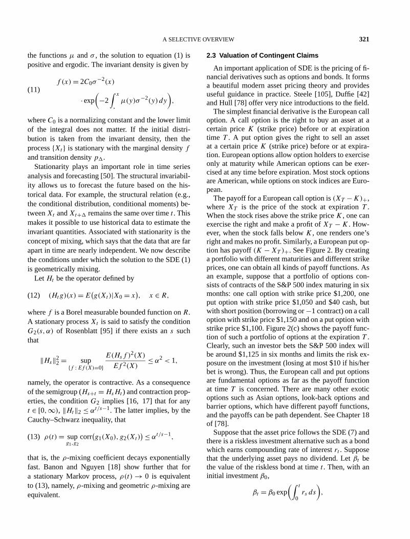
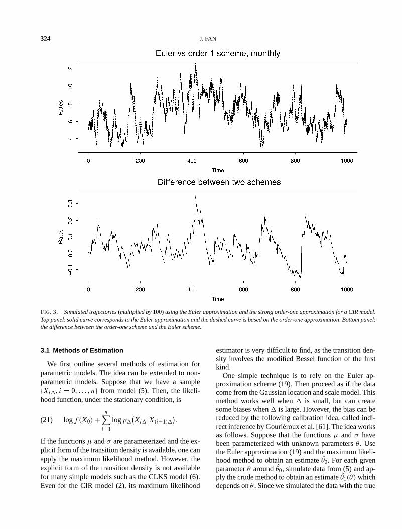
As an illustration, we consider the CIR model (7)with parametersκ = 0.21459, α = 0.08571, σ =0.07830 and� = 1/12. The model parameters aretaken from [30]. We simulated 1000 monthly data val-ues using both the Euler scheme (19) and the strongorder-one approximation (20) with the same randomshocks. Figure 3 depicts one of their trajectories. Thedifference is negligible. This is in line with the ob-servations made by Stanton [104] that as long as dataare sampled monthly or more frequently, the errors in-troduced by using the Euler approximation are verysmall for stochastic dynamics that are similar to theCIR model.

3. ESTIMATION OF RETURN AND VOLATILITYFUNCTIONS

There is a large literature on the estimation ofthe return and volatility functions. Early referencesinclude [93] and [94]. Some studies are based oncontinuously observed data while others are based ondiscretely observed data. For the latter, some regard�

tending to zero while others regard� fixed. We brieflyintroduce some of the ideas.

324 J. FAN

FIG. 3. Simulated trajectories(multiplied by100)using the Euler approximation and the strong order-one approximation for a CIR model.Top panel: solid curve corresponds to the Euler approximation and the dashed curve is based on the order-one approximation. Bottom panel:the difference between the order-one scheme and the Euler scheme.

3.1 Methods of Estimation

We first outline several methods of estimation forparametric models. The idea can be extended to non-parametric models. Suppose that we have a sample{Xi�, i = 0, . . . , n} from model (5). Then, the likeli-hood function, under the stationary condition, is

logf (X0) +n∑

i=1

logp�

(Xi�|X(i−1)�

).(21)

If the functionsµ andσ are parameterized and the ex-plicit form of the transition density is available, one canapply the maximum likelihood method. However, theexplicit form of the transition density is not availablefor many simple models such as the CLKS model (6).Even for the CIR model (2), its maximum likelihood

estimator is very difficult to find, as the transition den-sity involves the modified Bessel function of the firstkind.

One simple technique is to rely on the Euler ap-proximation scheme (19). Then proceed as if the datacome from the Gaussian location and scale model. Thismethod works well when� is small, but can createsome biases when� is large. However, the bias can bereduced by the following calibration idea, called indi-rect inference by Gouriéroux et al. [61]. The idea worksas follows. Suppose that the functionsµ andσ havebeen parameterized with unknown parametersθ . Usethe Euler approximation (19) and the maximum likeli-hood method to obtain an estimateθ0. For each givenparameterθ aroundθ0, simulate data from (5) and ap-ply the crude method to obtain an estimateθ1(θ) whichdepends onθ . Since we simulated the data with the true

A SELECTIVE OVERVIEW 325

parameterθ , the functionθ1(θ) tells us how to cali-brate the estimate. See Figure 4. Calibrate the estimatevia θ−1

1 (θ0), which improves the bias of the estimate.One drawback of this method is that it is intensive incomputation and the calibration cannot easily be donewhen the dimensionality of parametersθ is high.

Another method for bias reduction is to approximatethe transition density in (21) by a higher order approx-imation, and to then maximize the approximated like-lihood function. Such a scheme has been introducedby Aït-Sahalia [4, 5], who derives the expansion ofthe transition density around a normal density functionusing Hermite polynomials. The intuition behind suchan expansion is that the diffusion processXt+� − Xt

in (5) can be regarded as sum of many independentincrements with a very small step size and hence theEdgeworth expansion can be obtained for the distribu-tion of Xt+� − Xt givenXt . See also [43].

An “exact” approach is to use the method of moments.If the processXt is stationary as in the interest-ratemodels, the moment conditions can easily be derivedby observing

E

{lim�→0

�−1E[g(Xt+�) − g(Xt)|Xt ]}

= lim�→0

�−1E[g(Xt+�) − g(Xt)] = 0

for any functiong satisfying the regularity conditionthat the limit and the expectation are exchangeable.

The right-hand side is the expectation ofdg(Xt). ByItô’s formula (10), the above equation reduces to

E[g′(Xt)µ(Xt) + g′′(Xt)σ2(Xt)/2] = 0.(22)

For example, ifg(x) = exp(−ax) for some givena > 0, then

E exp(−aXt){µ(Xt) − aσ 2(Xt)/2} = 0.

This can produce an arbitrary number of equations bychoosing differenta’s. If the functionsµ andσ are pa-rameterized, the number of moment conditions can bemore than the number of equations. One way to effi-ciently use this is the generalized method of momentsintroduced by Hansen [65], minimizing a quadraticform of the discrepancies between the empirical andthe theoretical moments, a generalization of the clas-sical method of moments which solves the momentequations. The weighting matrix in the quadratic formcan be chosen to optimize the performance of the re-sulting estimator. To improve the efficiency of the es-timate, a large system of moments is needed. Thus,the generalized method of moments needs a large sys-tem of nonlinear equations which can be expensive incomputation. Further, the moment equations (22) useonly the marginal information of the process. Hence,the procedure is not efficient. For example, in theCKLS model (6),σ andκ are estimable via (22) onlythroughσ 2/κ .

FIG. 4. The idea of indirect inference. For each given trueθ , one obtains an estimate using the Euler approximation and the simulateddata. This gives a calibration curve as shown. Now for a given estimateθ0 = 3 based on the Euler approximation and real data, one finds thecalibrated estimateθ−1

1 (3) = 2.080.

326 J. FAN

3.2 Time-Homogeneous Model

The Euler approximation can easily be used toestimate the drift and diffusion nonparametrically.Let Yi� = �−1(X(i+1)� − Xi�) and Zi� =�−1(X(i+1)� − Xi�)2. Then

E(Yi�|Xi�) = µ(Xi�) + O(�)

and

E(Zi�|Xi�) = σ 2(Xi�) + O(�).

Thus,µ(·) and σ 2(·) can be approximately regardedas the regression functions ofYi� and Zi� on Xi�,respectively. Stanton [104] applies kernel regression[102, 107] to estimate the return and volatility func-tions. LetK(·) be a kernel function andh be a band-width. Stanton’s estimators are given by

µ(x) =∑n−1

i=0 Yi�Kh(Xi� − x)∑n−1i=0 Kh(Xi� − x)

and

σ 2(x) =∑n−1

i=0 Zi�Kh(Xi� − x)∑n−1i=0 Kh(Xi� − x)

,

whereKh(u) = h−1K(u/h) is a rescaled kernel. Theconsistency and asymptotic normality of the estimatorare studied in [15]. Fan and Yao [49] apply the locallinear technique (Section 6.3 in [50]) to estimate thereturn and volatility functions, under a slightly differ-ent setup. The local linear estimator [46] is given by

µ(x) =n−1∑i=0

Kn(Xi� − x, x)Yi�,(23)

where

Kn(u, x) = Kh(u)Sn,2(x) − uSn,1(x)

Sn,2(x)Sn,0(x) − Sn,1(x)2 ,(24)

with Sn,j (x) = ∑n−1i=0 Kh(Xi� − x)(Xi� − x)j , is the

equivalent kernel induced by the local linear fit. In con-trast to the kernel method, the local linear weights de-pend on bothXi andx. In particular, they satisfy

n−1∑i=1

Kn(Xi� − x, x) = 1

and

n−1∑i=1

Kn(Xi� − x, x)(Xi� − x) = 0.

These are the key properties for the bias reduction ofthe local linear method as demonstrated in [46]. Fur-ther, Fan and Yao [49] use the squared residuals

�−1(X(i+1)� − Xi� − µ(Xi�)�)2

rather thanZi� to estimate the volatility function. Thiswill further reduce the approximation errors in thevolatility estimation. They show further that the con-ditional variance function can be estimated as well asif the conditional mean function is known in advance.

Stanton [104] derives a higher-order approximationscheme up to order three in an effort to reduce bi-ases. He suggests that higher-order approximationsmust outperform lower-order approximations. To ver-ify such a claim, Fan and Zhang [53] derived the fol-lowing orderk approximation scheme:

E(Y ∗i�|Xi�) = µ(Xi�) + O(�k),

(25)E(Z∗

i�|Xi�) = σ 2(Xi�) + O(�k),

where

Y ∗i� = �−1

k∑j=1

ak,j

{X(i+j)� − Xi�

}

and

Z∗i� = �−1

k∑j=1

ak,j

{X(i+j)� − Xi�

}2

and the coefficientsak,j = (−1)j+1(kj

)/j are chosen to

make the approximation error in (25) of order�k . Forexample, the second approximation is

1.5(Xt+� − Xt) − 0.5(Xt+2� − Xt+�).

By using the independent increments of Brownian mo-tion, its variance is 1.52 + 0.52 = 2.5 times as large asthat of the first-order difference. Indeed, Fan and Zhang[53] show that while higher-order approximations givebetter approximation errors, we have to pay a huge pre-mium for variance inflation,

var(Y ∗i�|Xi�) = σ 2(Xi�)V1(k)�−1{1+ O(�)},

var(Z∗i�|Xi�) = 2σ 4(Xi�)V2(k){1+ O(�)},

where the variance inflation factorsV1(k) and V2(k)

are explicitly given by Fan and Zhang [53]. Table 1shows some of the numerical results for the varianceinflation factor.

The above theoretical results have also been veri-fied via empirical simulations in [53]. The problem isno monopoly for nonparametric fitting—it is shared by

A SELECTIVE OVERVIEW 327

TABLE 1Variance inflation factors by using higher-order differences

Order k

1 2 3 4 5

V1(k) 1.00 2.50 4.83 9.25 18.95V2(k) 1.00 3.00 8.00 21.66 61.50

the parametric methods. Therefore, the methods basedon higher-order differences should seldomly be usedunless the sampling interval is very wide (e.g., quar-terly data). It remains open whether it is possible toestimate nonparametrically the return and the volatilityfunctions without seriously inflating the variance withother higher-order approximation schemes.

As an illustration, we take the yields of the two-yearTreasury notes depicted in Figure 1. Figure 5 presentsnonparametrically estimated volatility functions, basedon orderk = 1 andk = 2 approximations. The locallinear fit is employed with the Epanechnikov kerneland bandwidthh = 0.35. It is evident that the order twoapproximation has higher variance than the order oneapproximation. In fact, the magnitude of variance in-flation is in line with the theoretical result: the increaseof the standard deviation is

√3 from order one to order

two approximation.Various discretization schemes and estimation meth-

ods have been proposed for the case with highfrequency data over a long time horizon. More pre-cisely, the studies are under the assumptions that�n → 0 andn�n → ∞. See, for example, [12, 27,39, 58, 59, 85, 109] and references therein. Arapis

FIG. 5. Nonparametric estimates of volatility based on order one and two differences. The bars represent two standard deviations aboveand below the estimated volatility. Top panel: order one fit. Bottom panel: order two fit.

328 J. FAN

and Gao [11] investigate the mean integrated squareerror of several methods for estimating the drift anddiffusion and compare their performances. Aït-Sahaliaand Mykland [9, 10] study the effects of random anddiscrete sampling when estimating continuous-timediffusions. Bandi and Nguyen [14] investigate smallsample behavior of nonparametric diffusion estima-tors. Thorough study of nonparametric estimation ofconditional variance functions can be found in [62, 69,91, 99]. In particular, Section 8.7 of [50] gives var-ious methods for estimating the conditional variancefunction. Wang [108] studies the relationship betweendiffusion and GARCH models.

3.3 Model Validation

Stanton [104] applies his kernel estimator to a Trea-sury bill data set and observes a nonlinear returnfunction in his nonparametric estimate, particularly inthe region where the interest rate is high (over 14%,say). This leads him to postulate the hypothesis thatthe return functions of short-term rates are nonlin-ear. Chapman and Pearson [30] study the finite sam-ple properties of Stanton’s estimator. By applying hisprocedure to the CIR model, they find that Stanton’sprocedure produces spurious nonlinearity, due to theboundary effect and the mean reversion.

Can we apply a formal statistics test toStanton’s hypothesis? The null hypothesis can sim-ply be formulated: the drift is of a linear form asin model (6). What is the alternative hypothesis? Forsuch a problem our alternative model is usually vague.Hence, it is natural to assume that the drift is a nonlin-ear smooth function. This becomes a testing problemwith a parametric null hypothesis versus a nonpara-metric alternative hypothesis. There is a large bodyof literature on this. The basic idea is to compute adiscrepancy measure between the parametric estimatesand nonparametric estimates and to reject the paramet-ric hypothesis when the discrepancy is large. See, forexample, the book by Hart [73].

In an effort to derive a generally applicable principle,Fan et al. [54] propose the generalized likelihood ra-tio (GLR) tests for parametric-versus-nonparametric ornonparametric-versus-parametric hypotheses. The ba-sic idea is to replace the maximum likelihood undera nonparametric hypothesis (which usually does notexist) by the likelihood under good nonparametric es-timates. Section 9.3 of [50] gives details on the im-plementation of the GLR tests, including estimatingP -values, bias reduction and bandwidth selection. Themethod has been successfully employed by Fan and

Zhang [53] for checking whether the return and volatil-ity functions possess certain parametric forms.

Another viable approach of model validation isto base it on the transition density. One can checkwhether the nonparametrically estimated transitiondensity is significantly different from the parametri-cally estimated one. Section 4.3 provides some addi-tional details. Another approach, proposed by Hongand Li [77], uses the fact that under the null hypothesisthe random variables{Zi} are a sequence of i.i.d. uni-form random variables whereZi = P(Xi�|X(i−1)�, θ)

and P(y|x, θ) is the transition distribution function.They propose to detect the departure from the nullhypothesis by comparing the kernel-estimated bivari-ate density of{(Zi,Zi+1)} with that of the uniformdistribution on the unit square. The transition-density-based approaches appear more elegant as they checksimultaneously the forms of drift and diffusion. How-ever, the transition density does often not admit ananalytic form and the tests can be computationally in-tensive.

3.4 Fixed Sampling Interval

For practical analysis of financial data, it is hard todetermine whether the sampling interval tends to zero.The key determination is whether the approximationerrors for small “�” are negligible. It is ideal when amethod is applicable whether or not “�” is small. Thiskind of method is possible, as demonstrated below.

The simplest problem to illustrate the idea is the ker-nel density estimation of the invariant density of thestationary process{Xt }. For the given sample{Xt�},the kernel density estimate for the invariant density is

f (x) = n−1n∑

i=1

Kh(Xi� − x),(26)

based on the discrete data{Xi�, i = 1, . . . , n}. Thismethod is valid for all�. It gives a consistent estimateof f as long as the time horizon is long:n� → ∞.We will refer to this kind of nonparametric method asstate-domain smoothing, as the procedure localizes inthe state variableXt . Various properties, including con-sistency and asymptotic normality, of the kernel esti-mator (26) are studied by Bandi [13] and Bandi andPhillips [15]. Bandi [13] also uses the estimator (26),which is the same as the local time of the processspending at a pointx except for a scaling constant, as adescriptive tool for potentially nonstationary diffusionprocesses.

Why can the state-domain smoothing methods beemployed as if the data were independent? This is due

A SELECTIVE OVERVIEW 329

to the fact that localizing in the state domain weakensthe correlation structure and that nonparametric esti-mates use essentially only local data. Hence many re-sults on nonparametric estimators for independent datacontinue to hold for dependent data as long as theirmixing coefficients decay sufficiently fast. As men-tioned at the end of Section 2.2, geometric mixing andmixing are equivalent for time-homogeneous diffusionprocesses. Hence, the mixing coefficients decay usu-ally sufficiently fast for theoretical investigation.

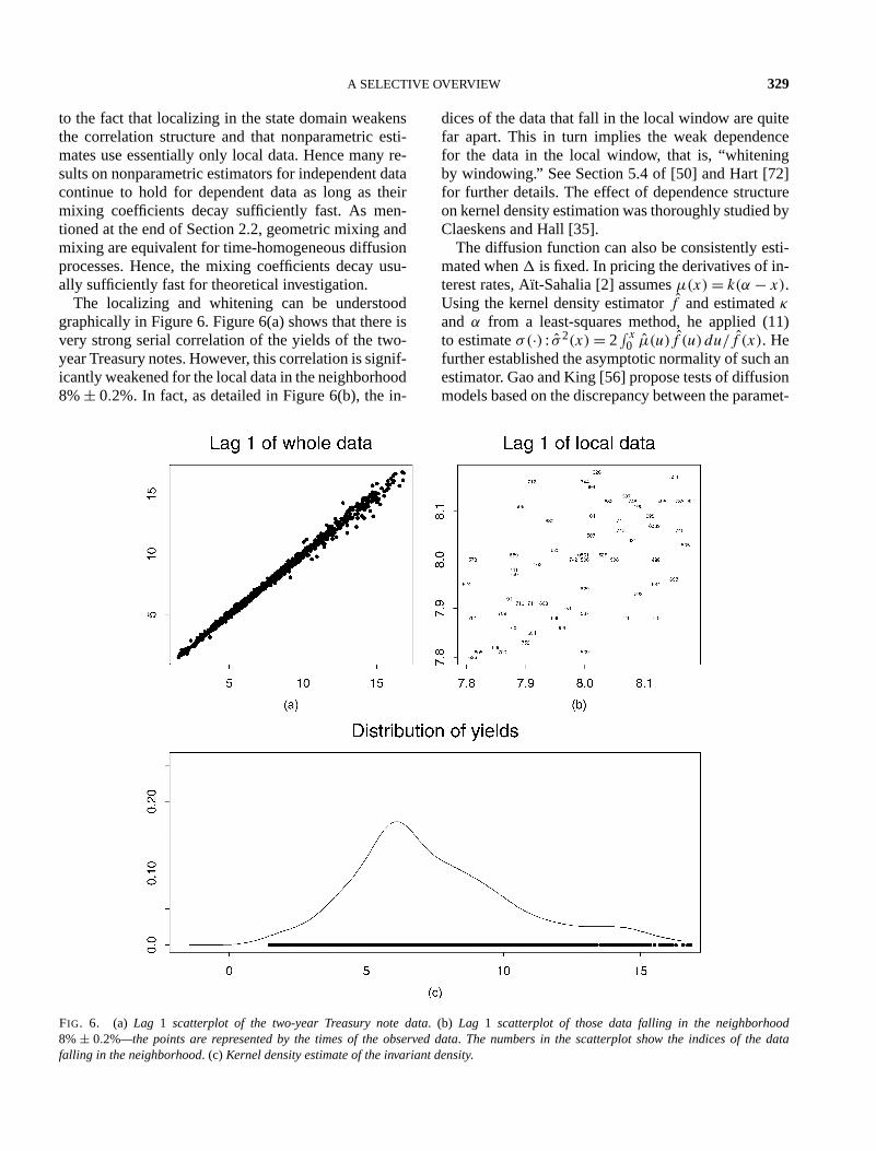
The localizing and whitening can be understoodgraphically in Figure 6. Figure 6(a) shows that there isvery strong serial correlation of the yields of the two-year Treasury notes. However, this correlation is signif-icantly weakened for the local data in the neighborhood8%± 0.2%. In fact, as detailed in Figure 6(b), the in-

dices of the data that fall in the local window are quitefar apart. This in turn implies the weak dependencefor the data in the local window, that is, “whiteningby windowing.” See Section 5.4 of [50] and Hart [72]for further details. The effect of dependence structureon kernel density estimation was thoroughly studied byClaeskens and Hall [35].

The diffusion function can also be consistently esti-mated when� is fixed. In pricing the derivatives of in-terest rates, Aït-Sahalia [2] assumesµ(x) = k(α − x).Using the kernel density estimatorf and estimatedκand α from a least-squares method, he applied (11)to estimateσ(·) : σ 2(x) = 2

∫ x0 µ(u)f (u) du/f (x). He

further established the asymptotic normality of such anestimator. Gao and King [56] propose tests of diffusionmodels based on the discrepancy between the paramet-

FIG. 6. (a) Lag 1 scatterplot of the two-year Treasury note data. (b) Lag 1 scatterplot of those data falling in the neighborhood8%± 0.2%—the points are represented by the times of the observed data. The numbers in the scatterplot show the indices of the datafalling in the neighborhood. (c) Kernel density estimate of the invariant density.

330 J. FAN

ric and nonparametric estimates of the invariant den-sity.

The Aït-Sahalia method [2] easily illustrates that thevolatility function can be consistently estimated forfixed �. However, we do not expect that it is effi-cient. Indeed, we use only the marginal information ofthe data. As shown in (21), almost all information iscontained in the transition densityp�(·|·). The tran-sition density can be estimated as in Section 4.2 be-low whether� is small or large. Since the transitiondensity and drift and volatility are in one-to-one cor-respondence for the diffusion process (5), the drift anddiffusion functions can be consistently estimated viainverting the relationship between the transition den-sity and the drift and diffusion functions.

There is no simple formula for expressing the driftand diffusion in terms of the transition density. The in-version is frequently carried out via a spectral analysisof the operatorH� = exp(�L), where the infinitesimaloperatorL is defined as

Lg(x) = σ 2(x)

2g′′(x) + µ(x)g′(x).

It has the property

Lg(x) = lim�→0

�−1[E{g(Xt+�)|Xt = x} − g(x)]by Itô’s formula (10). The operatorH� is the transitionoperator in that [see also (12)]

H�g(x) = E{g(X�)|X0 = x}.The works of Hansen and Scheinkman [66], Hansen,Scheinkman and Touzi [67] and Kessler and Sørensen[86] consist of the following idea. The first step is to es-timate the transition operatorH� from the data. Fromthe transition operator, one can identify the infinitesi-mal operatorL and hence the functionsµ(·) andσ(·).More precisely, letλ1 be the largest negative eigen-value of the operatorL with eigenfunctionξ1(x). ThenLξ1 = λ1ξ1, or equivalently,σ 2ξ ′′

1 + 2µξ ′1 = 2λ1ξ1.

This gives one equation ofµ andσ . Another equationcan be obtained via (11):(σ 2f )′ − 2µf = 0. Solvingthese two equations we obtain

σ 2(x) = 2λ1

∫ x

0ξ1(y)f (y) dy/[f (x)ξ1(x)]

and another explicit expression forµ(x). Using semi-group theory ([44], Theorem IV.3.7),ξ1 is also aneigenfunction ofH� with eigenvalue exp(�λ1). Hence,the proposal is to estimate the invariant densityf andthe transition densityp�(y|x), which implies the val-ues ofλ1 andξ1. Gobet [58] derives the optimal rate

of convergence for such a scheme, using a wavelet ba-sis. In particular, [58] shows that for fixed�, the op-timal rates of convergence forµ andσ are of ordersO(n−s/(2s+5)) andO(n−s/(2s+3)), respectively, wheres is the degree of smoothness ofµ andσ .

3.5 Time-Dependent Model

The time-dependent model (8) was introduced to ac-commodate the possibility of economic changes overtime. The coefficient functions in (8) are assumed tobe slowly time-varying and smooth. Nonparametrictechniques can be applied to estimate these coefficientfunctions. The basic idea is to localizing in time, re-sulting in a time-domain smoothing.

We first estimate the coefficient functionsα0(t)

andα1(t). For each given timet0, approximate the co-efficient functions locally by constants,α(t) ≈ a andβ(t) = b for t in a neighborhood oft0. Using the Eulerapproximation (19), we run a local regression: Mini-mize

n−1∑i=0

(Yi� − a − bXi�)2Kh(i� − t0)(27)

with respect toa and b. This results in an estimateα0(t0) = a and α1(t0) = b, where a and b are theminimizers of the local regression (27). Fan et al. [48]suggest using a one-sided kernel such asK(u) = (1−u2)I (−1 < u < 0) so that only the historical data inthe time interval(t0 − h, t0) are used in the above localregression. This facilitates forecasting and bandwidthselection. Our experience shows that there are no sig-nificant differences between nonparametric fitting withone-sided and two-sided kernels. We opt for local con-stant approximations instead of local linear approxi-mations in (27), since the local linear fit can createartificial albeit insignificant linear trends when the un-derlying functionsα0(t) and α1(t) are indeed time-independent. To appreciate this, for constant functionsα1 andα2 a large bandwidth will be chosen to reducethe variance in the estimation. This is in essence fittinga global linear regression by (27). If the local linear ap-proximations are used, since no variable selection pro-cedures have been incorporated in the local fitting (27),the slopes of the local linear approximations will not beestimated as zero and hence artificial linear trends willbe created for the estimated coefficients.

The coefficient functions in the volatility can be es-timated by the local approximated likelihood method.Let

Et = �−1/2{Xt+� − Xt − (α0(t) + α1(t)Xt

)�

}

A SELECTIVE OVERVIEW 331

be the normalized residuals. Then

Et ≈ β0(t)Xβ1(t)t εt .(28)

The conditional log-likelihood ofEt givenXt can eas-ily be obtained by the approximation (28). Using lo-cal constant approximations and incorporating the ker-nel weight, we obtain the local approximated likeli-hood at each time point and estimates of the functionsβ0(·) and β1(·) at that time point. This type of localapproximated-likelihood method is related to the gen-eralized method of moments of Hansen [65] and theideas of Florens-Zmirou [55] and Genon-Catalot andJacod [57].

Since the coefficient functions in both return andvolatility functions are estimated using only historicaldata, their bandwidths can be selected based on a formof the average prediction error. See Fan et al. [48] fordetails. The local least-squares regression can also beapplied to estimate the coefficient functionsβ0(t) andβ1(t) via the transformed model [see (28)]

log(E2t ) ≈ 2 logβ0(t) + β1(t) log(X2

t ) + log(ε2t ),

but we do not continue in this direction since the lo-cal least-squares estimate is known to be inefficient inthe likelihood context and the exponentiation of an es-timated coefficient function of logβ0(t) is unstable.

The question arises naturally if the coefficients inthe model (8) are really time-varying. This amounts,for example, to testingH0 :β0(t) = β0 andβ1(t) = β1.

Based on the GLR technique, Fan et al. [48] proposeda formal test for this kind of problem.

The coefficient functions in the semiparametricmodel (9) can also be estimated by using the profileapproximated-likelihood method. For each givenβ1,one can easily estimateβ0(·) via the approxima-tion (28), resulting in an estimateβ0(·;β1). Regardingthe nonparametric functionβ0(·) as being parameter-ized byβ0(·;β1), model (28) withβ1(t) ≡ β1 becomesa “synthesized” parametric model with unknownβ1.The parameterβ1 can be estimated by the maximum(approximated) likelihood method. Note thatβ1 is es-timated by using all the data points, whileβ0(t) =β0(t; β1) is obtained by using only the local datapoints. See [48] for details.

For other nonparametric methods of estimating vola-tility in time inhomogeneous models, see Härdle,Herwartz and Spokoiny [68] and Mercurio andSpokoiny [89]. Their methods are based on model (8)with α1(t) = β1(t) = 0.

3.6 State-Domain Versus Time-Domain Smoothing

So far, we have introduced both state- and time-domain smoothing. The former relies on the structuralinvariability implied by the stationarity assumption anddepends predominantly on the (remote) historical data.The latter uses the continuity of underlying parame-ters and concentrates basically on the recent data. Thisis illustrated in Figure 7 using the yields of the three-month Treasury bills from January 8, 1954 to July 16,

FIG. 7. Illustration of time- and state-domain smoothing using the yields of three-month Treasury bills. The state-domain smoothing islocalized in the horizontal bars, while the time-domain smoothing is concentrated in the vertical bars.

332 J. FAN

2004 sampled at weekly frequency. On December 28,1990, the interest rate was about 6.48%. To estimatethe drift and diffusion aroundx = 6.48, the state-domain smoothing focuses on the dynamics where in-terest rates are around 6.48%, the horizontal bar withinterest rates falling in 6.48%± 0.25%. The estimatedvolatility is basically the sample standard deviation ofthe differences{Xi� − X(i−1)�} within this horizon-tal bar. On the other hand, the time-domain smoothingfocuses predominantly on the recent history, say oneyear, as illustrated in the figure. The time-domain esti-mate of volatility is basically a sample standard devia-tion within the vertical bar.

For a given time series, it is hard to say which esti-mate is better. This depends on the underlying stochas-tic processes and also on the time when the forecast ismade. If the underlying process is continuous and sta-tionary, such as model (5), both methods are applica-ble. For example, standing at December 28, 1990, onecan forecast the volatility by using the sample standarddeviation in either the horizontal bar or the vertical bar.However, the estimated precision depends on the lo-cal data. Since the sample variance is basically linearin the squared differences{Z2

i�}, the standard errors ofboth estimates can be assessed and used to guide theforecasting.

For stationary diffusion processes, it is possible tointegrate both the time-domain and state-domain esti-mates. Note that the historical data (with interest ratesin 6.48%± 0.25%) are far apart in time from the dataused in the time-domain smoothing (vertical bar), ex-cept the last segment, which can be ignored in the state-domain fitting. The next-to-last segment with interestrates in 6.48%± 0.25% is May 11 to July 20, 1988,123 weeks prior to the last segment. Hence, these twoestimates are nearly independent. The integrated esti-mate is a linear combination of these two nearly in-dependent estimates. The weights can easily be cho-sen to minimize the variance of the integrated estima-tor, by using the assessed standard errors of the state-and time-domain estimators. The optimal weights areproportional to the variances of the two estimators,which depend on timet . This forms a dynamically inte-grated predictor for volatility estimation, as the optimalweights change over time.

3.7 Continuously Observed Data

At the theoretical level, one may also examine theproblem of estimating the drift and diffusion functionsassuming the whole process is observable up to timeT .

Let us assume again that the observed process{Xt } fol-lows the SDE (5). In this caseσ 2(Xt) is the derivativeof the quadratic variation process ofXt and hence isknown up to timeT . By (11), estimating the drift func-tion µ(x) is equivalent to estimating the invariant den-sity f . In fact,

µ(x) = [σ 2(x)f (x)]′/[2f (x)].(29)

The invariant densityf can easily be estimated bykernel density estimation. When� → 0, the summa-tion in (26) converges to

f (x) = T −1∫ T

0Kh(Xt − x)dt.(30)

This forms a kernel density estimate of the invari-ant density based on the continuously observed data.Thus, an estimator forµ(x) can be obtained bysubstituting f (x) into (29). Such an approach hasbeen employed by Kutoyants [88] and Dalalyan andKutoyants [40, 41]. They established the sharp asymp-totic minimax risk for estimating the invariant densityf and its derivative as well as the drift functionµ. Inparticular, the functionsf , f ′ andµ can be estimatedwith ratesT −1/2, T −2s/(2s+1) andT −2s/(2s+1), respec-tively, wheres is the degree of smoothness ofµ. Theseare the optimal rates of convergence.

An alternative approach is to estimate the drift func-tion directly from (23). By letting� → 0, one caneasily obtain a local linear regression estimator for con-tinuously observed data, which admits a similar formto (23) and (30). This is the approach that Spokoiny[103] used. He showed that this estimator attains theoptimal rate of convergence and established further adata-driven bandwidth such that the local linear esti-mator attains adaptive minimax rates.

4. ESTIMATION OF STATE PRICE DENSITIES ANDTRANSITION DENSITIES

The state price density (SPD) is the probability den-sity of the value of an asset under the risk-neutralworld (14) (see [38]) or equivalent martingale mea-sure [71]. It is directly related to the pricing of financialderivatives. It is the transition density ofXT givenX0under the equivalent martingaleQ. The SPD does notdepend on the payoff function and hence it can be usedto evaluate other illiquid derivatives, once it is esti-mated from more liquid derivatives. On the other hand,the transition density characterizes the probability lawof a Markovian process and hence is useful for validat-ing Markovian properties and parametric models.

A SELECTIVE OVERVIEW 333

4.1 Estimation of the State Price Density

For some specific models, the state price density canbe formed explicitly. For example, for the GBM (1)with a constant risk-free rater , according to (17), theSPD is log-normal with mean logx0 + (r − σ 2)/(2T )

and varianceσ 2.Assume that the SPDf ∗ exists. Then the European

call option can be expressed as

C = exp(−

∫ T

0rs ds

)∫ ∞K

(x − K)f ∗(x) dx.

See (14) (we have changed the notation fromP0 to C

to emphasize the price of the European call option).Hence,

f ∗(K) = exp(∫ T

0rs ds

)∂2C

∂K2 .(31)

This was observed by Breeden and Litzenberger [25].Thus, the state price density can be estimated from theEuropean call options with different strike prices. Withthe estimated state price density, one can price new orless liquid securities such as over-the-counter deriva-tives or nontraded options using formula (14).

In general, the price of a European call option de-pends on the current stock priceS, the strike priceK ,the time to maturityT , the risk-free interest rater anddividend yield rateδ. It can be written asC(S,K,T ,

r, δ). The exact form ofC, in general, is hard to de-termine unless we assume the Black–Scholes model.Based on historical data{(Ci, Si,Ki, Ti, ri, δi), i =1, . . . , n}, where Ci is the ith traded-option pricewith associated characteristics(Si,Ki, Ti, ri, δi), Aït-Sahalia and Lo [7] fit the nonparametric regression

Ci = C(Si,Ki, Ti, ri, δi) + εi

to obtain an estimate of the functionC and hence theSPDf ∗.

Due to the curse of dimensionality, the five-dimen-sional nonparametric function cannot be estimated wellwith practical range of sample sizes. Aït-Sahalia andLo [7] realized that and proposed a few dimensionalityreduction methods. First, by assuming that the optionprice depends only on the futures priceF = S exp((r −δ)T ), namely,

C(S,K,T , r, δ) = C(F,K,T , r)

(the Black–Scholes formula satisfies such an assump-tion), they reduced the dimensionality from five to four.By assuming further that the option-pricing function ishomogeneous of degree one inF andK , namely,

C(S,K,T , r, δ) = KC(F/K,T , r),

they reduced the dimensionality to three. Aït-Sahaliaand Lo [7] imposed a semiparametric form on the pric-ing formula,

C(S,K,T , r, δ) = CBS(F,K,T , r, σ (F,K,T )

),

whereCBS(F,K,T , r, σ ) is the Black–Scholes pricingformula given in (18) andσ(F,K,T ) is the impliedvolatility, computed by inverting the Black–Scholesformula. Thus, the problem becomes one of nonpara-metrically estimating the implied volatility functionσ(F,K,T ). This is estimated by using a nonparamet-ric regression technique from historical data, namely,

σi = σ(Fi,Ki, Ti) + εi,

whereσi is the implied volatility ofCi , by invertingthe Black–Scholes formula. By assuming further thatσ(F,K,T ) = σ(F/K,T ), the dimensionality is re-duced to two. This is one of the options in [4].

The state price densityf ∗ is nonnegative and hencethe functionC should be convex in the strike priceK .Aït-Sahalia and Duarte [6] propose to estimate the op-tion price under the convexity constraint using a locallinear estimator. See also [70] for a related approach.

4.2 Estimation of Transition Densities

The transition density of a Markov process charac-terizes the law of the process, except the initial distrib-ution. It provides useful tools for checking whether ornot such a process follows a certain SDE and for statis-tical estimation and inference. It is the state price den-sity of the price process under the risk neutral world. Ifsuch a process were observable, the state price densitywould be estimated using the methods to be introduced.

Assume that we have a sample{Xi�, i = 0, . . . , n}from model (5). The “double-kernel” method of Fan,Yao and Tong [51] is to observe that

E{Wh2(Xi� − y)|X(i−1)� = x

} ≈ p�(y|x)(32)

ash2 → 0,

for a kernel functionW . Thus, the transition densityp�(y|x) can be regarded approximately as the non-parametric regression function of the response variableWh2(Xi� − y) onX(i−1)�. An application of the locallinear estimator (23) yields

p�(y|x) =n∑

i=1

Kn

(X(i−1)� − x, x

)(33)

· Wh2(Xi� − y),

334 J. FAN

where the equivalent kernelKn(u, x) was definedin (24). Fan, Yao and Tong [51] establish the asymp-totic normality of such an estimator under stationar-ity and ρ-mixing conditions [necessarily decaying atgeometric rate for SDE (5)], which gives explicitlythe asymptotic bias and variance of the estimator. Seealso Section 6.5 of [50]. The cross-validation idea ofRudemo [98] and Bowman [24] can be extended toselect bandwidths for estimating conditional densities.See [52, 63].

The transition distribution can be estimated by in-tegrating the estimator (33) overy. By lettingh2 → 0,the estimator is the regression of the indicatorI (Xi� <

y) on X(i−1)�. Alternative estimators can be obtainedby an application of the local logistic regression andadjusted Nadaraya–Watson method of Hall et al. [64].

Early references on the estimation of the transitiondistributions and densities include [96, 97] and [95].

4.3 Inferences Based on Transition Densities

With the estimated transition density, one can nowverify whether parametric models such as (1)–(3), (6)are consistent with the observed data. Letp�,θ (y|x)

be the transition density under a parametric diffusionmodel. For example, for the CIR model (2), the pa-rameterθ = (κ,α,σ ). As in (21), ignoring the initialvalueX0, the parameterθ can be estimated by maxi-mizing

�(p�,θ ) =n∑

i=1

logp�,θ

(Xi�|X(i−1)�

).

Let θ be the maximum likelihood estimator. By thespirit of the GLR of Fan et al. [54], the GLR test forthe null hypothesisH0 :p�(y|x) = p�,θ (y|x) is

GLR= �(p�) − �(p�,θ

),

where p is a nonparametric estimate of the transi-tion density. Since the transition density cannot be es-timated well over the region where data are sparse(usually at boundaries of the process), we need totruncate the nonparametric (and simultaneously para-metric) evaluation of the likelihood at appropriate in-tervals.

In addition to employing the GLR test, one can alsocompare directly the difference between the paramet-ric and nonparametric fits, resulting in test statisticssuch as‖p� − p

�,θ‖2 and‖P� − P

�,θ‖2 for an ap-

propriate norm‖ · ‖, whereP� andP�,θ

are the esti-mates of the cumulative transition distributions underrespectively the parametric and nonparametric models.

The transition density-based methods depend on twobandwidths and are harder to implement. Indeed, theirnull distributions are harder to determine than thosebased on the transition distribution methods. In com-parison with the invariant density-based approach ofArapis and Gao [11], it is consistent against a muchlarger family of alternatives.

One can also use the transition density to testwhether an observed series is Markovian (from per-sonal communication with Yacine Aït-Sahalia). For ex-ample, if a process{Xi�} is Markovian, then

p2�(y|x) =∫ +∞−∞

p�(y|z)p�(z|x)dz.

Thus, one can use the distance betweenp2�(y|x) and∫ +∞−∞ p�(y|z)p�(z|x)dz as a test statistic.The transition density can also be used for parameter

estimation. One possible approach is to find the para-meter which minimizes the distance‖P� − P�,θ‖. Inthis case, the bandwidth should be chosen to optimizethe performance for estimatingθ . The approach is ap-plicable whether or not� → 0.

5. CONCLUDING REMARKS

Enormous efforts in financial econometrics havebeen made in modeling the dynamics of stock pricesand bond yields. There are directly related to pricingderivative securities, proprietary trading and portfo-lio management. Various parametric models have beenproposed to facilitate mathematical derivations. Theyhave risks that misspecifications of models lead to er-roneous pricing and hedging strategies. Nonparamet-ric models provide a powerful and flexible treatment.They aim at reducing modeling biases by increasingsomewhat the variances of resulting estimators. Theyprovide an elegant method for validating or suggestinga family of parametric models.

The versatility of nonparametric techniques in fi-nancial econometrics has been demonstrated in thispaper. They are applicable to various aspects of dif-fusion models: drift, diffusion, transition densities andeven state price densities. They allow us to examinewhether the stochastic dynamics for stocks and bondsare time varying and whether famous parametric mod-els are consistent with empirical financial data. Theypermit us to price illiquid or nontraded derivatives fromliquid derivatives.

The applications of nonparametric techniques in fi-nancial econometrics are far wider than what has beenpresented. There are several areas where nonparamet-ric methods have played a pivotal role. One example

A SELECTIVE OVERVIEW 335

is to test various versions of capital asset pricing mod-els (CAPM) and their related stochastic discount mod-els [36]. See, for example, the research manuscriptby Chen and Ludvigson [34] in this direction. An-other important class of models are stochastic volatil-ity models [19, 101], where nonparametric methodscan be also applied. The nonparametric techniqueshave been prominently featured in the RiskMetrics ofJ. P. Morgan. It can be employed to forecast the risksof portfolios. See, for example, [8, 32, 33, 47, 82] forrelated nonparametric techniques on risk management.

ACKNOWLEDGMENTS

The author gratefully acknowledges various discus-sions with Professors Yacine Aït-Sahalia and Jia-anYan and helpful comments of the editors and review-ers that led to significant improvement of the presenta-tion of this paper. This research was supported in partby NSF Grant DMS-03-55179 and a direct allocationRGC grant of the Chinese University of Hong Kong.

REFERENCES

[1] A HN, D. H. and GAO, B. (1999). A parametric nonlinearmodel of term structure dynamics.Review of Financial Stud-ies12 721–762.

[2] A ÏT-SAHALIA , Y. (1996). Nonparametric pricing of interestrate derivative securities.Econometrica64 527–560.

[3] A ÏT-SAHALIA , Y. (1996). Testing continuous-time modelsof the spot interest rate.Review of Financial Studies9 385–426.

[4] A ÏT-SAHALIA , Y. (1999). Transition densities for inter-est rate and other nonlinear diffusions.J. Finance 541361–1395.

[5] A ÏT-SAHALIA , Y. (2002). Maximum likelihood estimationof discretely sampled diffusions: A closed-form approxima-tion approach.Econometrica70 223–262.

[6] A ÏT-SAHALIA , Y. and DUARTE, J. (2003). Nonparametricoption pricing under shape restrictions.J. Econometrics1169–47.

[7] A ÏT-SAHALIA , Y. and LO, A. W. (1998). Nonparametricestimation of state-price densities implicit in financial assetprices.J. Finance53 499–547.

[8] A ÏT-SAHALIA , Y. and LO, A. W. (2000). Nonparametricrisk management and implied risk aversion.J. Econometrics94 9–51.

[9] A ÏT-SAHALIA , Y. and MYKLAND , P. (2003). The effects ofrandom and discrete sampling when estimating continuous-time diffusions.Econometrica71 483–549.

[10] AÏT-SAHALIA , Y. and MYKLAND , P. (2004). Estimatorsof diffusions with randomly spaced discrete observations:A general theory.Ann. Statist.32 2186–2222.

[11] ARAPIS, M. and GAO, J. (2004). Nonparametric kernel es-timation and testing in continuous-time financial economet-rics. Unpublished manuscript.

[12] ARFI, M. (1998). Non-parametric variance estimation fromergodic samples.Scand. J. Statist.25 225–234.

[13] BANDI , F. (2002). Short-term interest rate dynamics: A spa-tial approach.J. Financial Economics65 73–110.

[14] BANDI , F. and NGUYEN, T. (1999). Fully nonparametricestimators for diffusions: A small sample analysis. Unpub-lished manuscript.

[15] BANDI , F. and PHILLIPS, P. C. B. (2003). Fully nonpara-metric estimation of scalar diffusion models.Econometrica71 241–283.

[16] BANON, G. (1977). Estimation non paramétrique de densitéde probabilité pour les processus de Markov. Thése, Univ.Paul Sabatier de Toulouse, France.

[17] BANON, G. (1978). Nonparametric identification for diffu-sion processes.SIAM J. Control Optim.16 380–395.

[18] BANON, G. and NGUYEN, H. T. (1981). Recursive estima-tion in diffusion models.SIAM J. Control Optim.19 676–685.

[19] BARNDOFF-NIELSEN, O. E. and SHEPHARD, N. (2001).Non-Gaussian Ornstein–Uhlenbeck-based models and someof their uses in financial economics (with discussion).J. R.Stat. Soc. Ser. B Stat. Methodol.63 167–241.

[20] BINGHAM , N. H. and KIESEL, R. (1998).Risk-NeutralValuation: Pricing and Hedging of Financial Derivatives.Springer, New York.

[21] BLACK , F., DERMAN, E. and TOY, W. (1990). A one-factormodel of interest rates and its application to Treasury bondoptions.Financial Analysts Journal46(1) 33–39.

[22] BLACK , F. and KARASINSKI, P. (1991). Bond and optionpricing when short rates are lognormal.Financial AnalystsJournal47(4) 52–59.

[23] BLACK , F. and SCHOLES, M. (1973). The pricing of op-tions and corporate liabilities.J. Political Economy81 637–654.

[24] BOWMAN, A. W. (1984). An alternative method of cross-validation for the smoothing of density estimates.Bio-metrika71 353–360.

[25] BREEDEN, D. and LITZENBERGER, R. H. (1978). Prices ofstate-contingent claims implicit in option prices.J. Business51 621–651.

[26] CAI , Z., FAN, J. and YAO, Q. (2000). Functional-coefficient regression models for nonlinear time series.J.Amer. Statist. Assoc.95 941–956.

[27] CAI , Z. and HONG, Y. (2003). Nonparametric methods incontinuous-time finance: A selective review. InRecent Ad-vances and Trends in Nonparametric Statistics(M. G. Akri-tas and D. N. Politis, eds.) 283–302. North-Holland, Ams-terdam.

[28] CAMPBELL, J. Y., LO, A. W. and MACKINLAY, A. C.(1997).The Econometrics of Financial Markets. PrincetonUniv. Press.

[29] CHAN, K. C., KAROLYI , G. A., LONGSTAFF, F. A. andSANDERS, A. B. (1992). An empirical comparison of alter-native models of the short-term interest rate.J. Finance471209–1227.

[30] CHAPMAN, D. A. and PEARSON, N. D. (2000). Is the shortrate drift actually nonlinear?J. Finance55 355–388.

[31] CHEN, R. and TSAY, R. S. (1993). Functional-coefficientautoregressive models.J. Amer. Statist. Assoc.88 298–308.

336 J. FAN

[32] CHEN, S. X. (2005). Nonparametric estimation of expectedshortfall.Econometric Theory. To appear.

[33] CHEN, S. X. and TANG, C. Y. (2005). Nonparametric in-ference of value-at-risk for dependent financial returns.J.Financial Econometrics3 227–255.

[34] CHEN, X. and LUDVIGSON, S. (2003). Land of Addicts?An empirical investigation of habit-based asset pricingmodel. Unpublished manuscript.

[35] CLAESKENS, G. and HALL , P. (2002). Effect of depen-dence on stochastic measures of accuracy of density esti-mators.Ann. Statist.30 431–454.

[36] COCHRANE, J. H. (2001).Asset Pricing. Princeton Univ.Press.

[37] COX, J. C., INGERSOLL, J. E. and ROSS, S. A. (1985).A theory of the term structure of interest rates.Econometrica53 385–407.

[38] COX, J. C. and ROSS, S. (1976). The valuation of optionsfor alternative stochastic processes.J. Financial Economics3 145–166.

[39] DACUNHA-CASTELLE, D. and FLORENS, D. (1986). Esti-mation of the coefficients of a diffusion from discrete obser-vations.Stochastics19 263–284.

[40] DALALYAN , A. S. and KUTOYANTS, Y. A. (2002). Asymp-totically efficient trend coefficient estimation for ergodic dif-fusion.Math. Methods Statist.11 402–427.

[41] DALALYAN , A. S. and KUTOYANTS, Y. A. (2003). Asymp-totically efficient estimation of the derivative of the invariantdensity.Stat. Inference Stoch. Process.6 89–107.

[42] DUFFIE, D. (2001).Dynamic Asset Pricing Theory, 3rd ed.Princeton Univ. Press.

[43] EGOROV, A. V., L I , H. and XU, Y. (2003). Maximumlikelihood estimation of time-inhomogeneous diffusions.J.Econometrics114 107–139.

[44] ENGEL, K.-J. and NAGEL, R. (2000). One-ParameterSemigroups for Linear Evolution Equations. Springer,Berlin.

[45] ENGELBERT, H. J. and SCHMIDT, W. (1984). On one-dimensional stochastic differential equations with general-ized drift. Stochastic Differential Systems. Lecture Notes inControl and Inform. Sci.69 143–155. Springer, Berlin.

[46] FAN, J. (1992). Design-adaptive nonparametric regression.J. Amer. Statist. Assoc.87 998–1004.

[47] FAN, J. and GU, J. (2003). Semiparametric estimation ofvalue-at-risk.Econom. J.6 261–290.

[48] FAN, J., JIANG, J., ZHANG, C. and ZHOU, Z. (2003).Time-dependent diffusion models for term structure dynam-ics.Statist. Sinica13 965–992.

[49] FAN, J. and YAO, Q. (1998). Efficient estimation of con-ditional variance functions in stochastic regression.Bio-metrika85 645–660.

[50] FAN, J. and YAO, Q. (2003).Nonlinear Time Series: Non-parametric and Parametric Methods. Springer, New York.

[51] FAN, J., YAO, Q. and TONG, H. (1996). Estimation of con-ditional densities and sensitivity measures in nonlinear dy-namical systems.Biometrika83 189–206.

[52] FAN, J. and YIM , T. H. (2004). A crossvalidation methodfor estimating conditional densities.Biometrika91 819–834.

[53] FAN, J. and ZHANG, C. (2003). A re-examination of diffu-sion estimators with applications to financial model valida-tion. J. Amer. Statist. Assoc.98 118–134.

[54] FAN, J., ZHANG, C. and ZHANG, J. (2001). Generalizedlikelihood ratio statistics and Wilks phenomenon.Ann. Sta-tist. 29 153–193.

[55] FLORENS-ZMIROU, D. (1993). On estimating the diffusioncoefficient from discrete observations.J. Appl. Probab.30790–804.

[56] GAO, J. and KING, M. (2004). Adaptive testing incontinuous-time diffusion models.Econometric Theory20844–882.

[57] GENON-CATALOT, V. and JACOD, J. (1993). On the estima-tion of the diffusion coefficient for multi-dimensional diffu-sion processes.Ann. Inst. H. Poincaré Probab. Statist.29119–151.

[58] GOBET, E. (2002). LAN property for ergodic diffusionswith discrete observations.Ann. Inst. H. Poincaré Probab.Statist.38 711–737.

[59] GOBET, E., HOFFMANN, M. and REISS, M. (2004). Non-parametric estimation of scalar diffusions based on low fre-quency data.Ann. Statist.32 2223–2253.

[60] GOURIÉROUX, C. and JASIAK , J. (2001).Financial Econo-metrics: Problems, Models, and Methods. Princeton Univ.Press.

[61] GOURIÉROUX, C., MONFORT, A. and RENAULT, E.(1993). Indirect inference.J. Appl. Econometrics8 suppl.S85–S118.

[62] HALL , P. and CARROLL, R. J. (1989). Variance functionestimation in regression: The effect of estimating the mean.J. Roy. Statist. Soc. Ser. B51 3–14.

[63] HALL , P., RACINE, J. and LI, Q. (2004). Cross-validationand the estimation of conditional probability densities.J.Amer. Statist. Assoc.99 1015–1026.

[64] HALL , P., WOLFF, R. C. L. and YAO, Q. (1999). Methodsfor estimating a conditional distribution function.J. Amer.Statist. Assoc.94 154–163.

[65] HANSEN, L. P. (1982). Large sample properties of gen-eralized method of moments estimators.Econometrica501029–1054.

[66] HANSEN, L. P. and SCHEINKMAN , J. A. (1995). Back tothe future: Generating moment implications for continuous-time Markov processes.Econometrica63 767–804.

[67] HANSEN, L. P., SCHEINKMAN , J. A. and TOUZI, N.(1998). Spectral methods for identifying scalar diffusions.J. Econometrics86 1–32.

[68] HÄRDLE, W., HERWARTZ, H. and SPOKOINY, V. (2003).Time inhomogeneous multiple volatility modelling.J. Fi-nancial Econometrics1 55–95.

[69] HÄRDLE, W. and TSYBAKOV, A. B. (1997). Local polyno-mial estimators of the volatility function in nonparametricautoregression.J. Econometrics81 223–242.

[70] HÄRDLE, W. and YATCHEW, A. (2002). Dynamicnonparametric state price density estimation using con-strained least-squares and the bootstrap. Discussion pa-per 16, Quantification and Simulation of EconomicsProcesses, Humboldt-Universität zu Berlin.

[71] HARRISON, J. M. and KREPS, D. (1979). Martingales andarbitrage in multiperiod securities markets.J. Econom. The-ory 2 381–408.

[72] HART, J. D. (1996). Some automated methods of smoothingtime-dependent data.Nonparametr. Statist.6 115–142.

A SELECTIVE OVERVIEW 337

[73] HART, J. D. (1997).Nonparametric Smoothing and Lack-of-Fit Tests. Springer, New York.

[74] HASTIE, T. J. and TIBSHIRANI, R. J. (1993). Varying-coefficient models (with discussion).J. Roy. Statist. Soc. Ser.B. 55 757–796.

[75] HO, T. S. Y. and LEE, S.-B. (1986). Term structure move-ments and pricing interest rate contingent claims.J. Finance41 1011–1029.

[76] HONG, Y. and LEE, T.-H. (2003). Inference on predictabil-ity of foreign exchange rates via generalized spectrum andnonlinear time series models.Review of Economics and Sta-tistics85 1048–1062.

[77] HONG, Y. and LI, H. (2005). Nonparametric specificationtesting for continuous-time models with applications to termstructure of interest rates.Review of Financial Studies1837–84.

[78] HULL , J. (2003).Options, Futures, and Other Derivatives,5th ed. Prentice Hall, Upper Saddle River, NJ.

[79] HULL , J. and WHITE, A. (1990). Pricing interest-rate-derivative securities.Review of Financial Studies3 573–592.

[80] ITÔ, K. (1942). Differential equations determining Markovprocesses.Zenkoku Shijo Sugaku Danwakai244 1352–1400. (In Japanese.)

[81] ITÔ, K. (1946). On a stochastic integral equation.Proc.Japan Acad.22 32–35.

[82] JORION, P. (2000).Value at Risk: The New Benchmark forManaging Financial Risk, 2nd ed. McGraw–Hill, New York.

[83] KALLENBERG, O. (2002).Foundations of Modern Proba-bility, 2nd ed. Springer, New York.

[84] KARATZAS, I. and SHREVE, S. E. (1991).Brownian Mo-tion and Stochastic Calculus, 2nd ed. Springer, New York.

[85] KESSLER, M. (1997). Estimation of an ergodic diffusionfrom discrete observations.Scand. J. Statist.24 211–229.

[86] KESSLER, M. and SØRENSEN, M. (1999). Estimating equa-tions based on eigenfunctions for a discretely observed dif-fusion process.Bernoulli 5 299–314.

[87] KLOEDEN, P. E., PLATEN, E., SCHURZ, H. andSØRENSEN, M. (1996). On effects of discretization on es-timators of drift parameters for diffusion processes.J. Appl.Probab.33 1061–1076.

[88] KUTOYANTS, Y. A. (1998). Efficient density estimation forergodic diffusion processes.Stat. Inference Stoch. Process.1 131–155.

[89] MERCURIO, D. and SPOKOINY, V. (2004). Statistical infer-ence for time-inhomogeneous volatility models.Ann. Statist.32 577–602.

[90] MERTON, R. (1973). Theory of rational option pricing.BellJ. Econom. Management Sci.4 141–183.

[91] MÜLLER, H.-G. and STADTMÜLLER , U. (1987). Estima-tion of heteroscedasticity in regression analysis.Ann. Statist.15 610–625.

[92] OSBORNE, M. F. M. (1959). Brownian motion in the stockmarket.Operations Res.7 145–173.

[93] PHAM , D. T. (1981). Nonparametric estimation of the driftcoefficient in the diffusion equation.Math. Operations-forsch. Statist. Ser. Statist.12 61–73.

[94] PRAKASA RAO, B. L. S. (1985). Estimation of the drift fordiffusion process.Statistics16 263–275.

[95] ROSENBLATT, M. (1970). Density estimates and Markovsequences. InNonparametric Techniques in Statistical In-ference(M. L. Puri, ed.) 199–213. Cambridge Univ. Press.

[96] ROUSSAS, G. G. (1969). Nonparametric estimation inMarkov processes.Ann. Inst. Statist. Math.21 73–87.

[97] ROUSSAS, G. G. (1969). Nonparametric estimation of thetransition distribution function of a Markov process.Ann.Math. Statist.40 1386–1400.

[98] RUDEMO, M. (1982). Empirical choice of histograms andkernel density estimators.Scand. J. Statist.9 65–78.

[99] RUPPERT, D., WAND, M. P., HOLST, U. and HÖSSJER,O. (1997). Local polynomial variance function estimation.Technometrics39 262–273.

[100] SCHURZ, H. (2000). Numerical analysis of stochastic dif-ferential equations without tears. InHandbook of StochasticAnalysis and Applications(D. Kannan and V. Lakshmikan-tham, eds.) 237–359. Dekker, New York.

[101] SHEPHARD, N., ed. (2005).Stochastic Volatility: SelectedReadings. Oxford Univ. Press.

[102] SIMONOFF, J. S. (1996).Smoothing Methods in Statistics.Springer, New York.

[103] SPOKOINY, V. (2000). Adaptive drift estimation for non-parametric diffusion model.Ann. Statist.28 815–836.

[104] STANTON, R. (1997). A nonparametric model of term struc-ture dynamics and the market price of interest rate risk.J.Finance52 1973–2002.

[105] STEELE, J. M. (2001).Stochastic Calculus and FinancialApplications. Springer, New York.

[106] VASICEK, O. A. (1977). An equilibrium characterization ofthe term structure.J. Financial Economics5 177–188.

[107] WAND, M. P. and JONES, M. C. (1995).Kernel Smoothing.Chapman and Hall, London.

[108] WANG, Y. (2002). Asymptotic nonequivalence of GARCHmodels and diffusions.Ann. Statist.30 754–783.

[109] YOSHIDA, N. (1992). Estimation for diffusion processesfrom discrete observations.J. Multivariate Anal. 41220–242.