statistical science a selective overview of nonparametric methods...

Statistical Science2005, Vol. 20, No. 4, 317–337DOI 10.1214/088342305000000412© Institute of Mathematical Statistics, 2005

A Selective Overview of NonparametricMethods in Financial EconometricsJianqing Fan

Abstract. This paper gives a brief overview of the nonparametric techniquesthat are useful for financial econometric problems. The problems include es-timation and inference for instantaneous returns and volatility functions oftime-homogeneous and time-dependent diffusion processes, and estimationof transition densities and state price densities. We first briefly describe theproblems and then outline the main techniques and main results. Some use-ful probabilistic aspects of diffusion processes are also briefly summarized tofacilitate our presentation and applications.

Key words and phrases:Asset pricing, diffusion, drift, GLR tests, simu-lations, state price density, time-inhomogeneous model, transition density,volatility.

1. INTRODUCTION

Technological innovation and trade globalizationhave brought us into a new era of financial markets.Over the last three decades, a large number of newfinancial products have been introduced to meet cus-tomers’ demands. An important milestone occurred in1973 when the world’s first options exchange openedin Chicago. That same year, Black and Scholes [23]published their famous paper on option pricing andMerton [90] launched the general equilibrium modelfor security pricing, two important landmarks for mod-ern asset pricing. Since then the derivative marketshave experienced extraordinary growth. Professionalsin finance now routinely use sophisticated statisticaltechniques and modern computational power in portfo-lio management, securities regulation, proprietary trad-ing, financial consulting and risk management.

Financial econometrics is an active field that inte-grates finance, economics, probability, statistics andapplied mathematics. This is exemplified by the booksby Campbell, Lo and MacKinlay [28], Gouriérouxand Jasiak [60] and Cochrane [36]. Financial activitiesgenerate many new problems, economics provides use-ful theoretical foundation and guidance, and quantita-

Jianqing Fan is Professor, Benheim Center of Financeand Department of Operations Research and FinancialEngineering, Princeton University, Princeton, NewJersey 08544, USA (e-mail: [email protected]).

tive methods such as statistics, probability and appliedmathematics are essential tools to solve the quantitativeproblems in finance. To name a few, complex finan-cial products pose new challenges on their valuationand risk management. Sophisticated stochastic mod-els have been introduced to capture the salient featuresof underlying economic variables and to price deriva-tives of securities. Statistical tools are used to identifyparameters of stochastic models, to simulate complexfinancial systems and to test economic theories via em-pirical financial data.

An important area of financial econometrics is studyof the expected returns and volatilities of the price dy-namics of stocks and bonds. Returns and volatilitiesare directly related to asset pricing, proprietary trad-ing, security regulation and portfolio management. Toachieve these objectives, the stochastic dynamics ofunderlying state variables should be correctly speci-fied. For example, option pricing theory allows oneto value stock or index options and hedge against therisks of option writers once a model for the dynamicsof underlying state variables is given. See, for exam-ple, the books on mathematical finance by Binghamand Kiesel [20], Steele [105] and Duffie [42]. Yet manyof the stochastic models in use are simple and conve-nient ones to facilitate mathematical derivations andstatistical inferences. They are not derived from anyeconomics theory and hence cannot be expected to fitall financial data. Thus, while the pricing theory gives

317

318 J. FAN

spectacularly beautiful formulas when the underlyingdynamics is correctly specified, it offers little guid-ance in choosing or validating a model. There is al-ways the danger that misspecification of a model leadsto erroneous valuation and hedging strategies. Hence,there are genuine needs for flexible stochastic model-ing. Nonparametric methods offer a unified and eleganttreatment for such a purpose.

Nonparametric approaches have recently been intro-duced to estimate return, volatility, transition densitiesand state price densities of stock prices and bond yields(interest rates). They are also useful for examining theextent to which the dynamics of stock prices and bondyields vary over time. They have immediate applica-tions to the valuation of bond price and stock optionsand management of market risks. They can also be em-ployed to test economic theory such as the capital assetpricing model and stochastic discount model [28] andanswer questions such as if the geometric Brownianmotion fits certain stock indices, whether the Cox–Ingersoll–Ross model fits yields of bonds, and if in-terest rate dynamics evolve with time. Furthermore,based on empirical data, one can also fit directly theobserved option prices with their associated character-istics such as strike price, the time to maturity, risk-freeinterest rate, dividend yield and see if the option pricesare consistent with the theoretical ones. Needless tosay, nonparametric techniques will play an increas-ingly important role in financial econometrics, thanksto the availability of modern computing power and thedevelopment of financial econometrics.

The paper is organized as follows. We first intro-duce in Section 2 some useful stochastic models formodeling stock prices and bond yields and then brieflyoutline some probabilistic aspects of the models. InSection 3 we review nonparametric techniques used forestimating the drift and diffusion functions, based oneither discretely or continuously observed data. In Sec-tion 4 we outline techniques for estimating state pricedensities and transition densities. Their applications inasset pricing and testing for parametric diffusion mod-els are also introduced. Section 5 makes some conclud-ing remarks.

2. STOCHASTIC DIFFUSION MODELS

Much of financial econometrics is concerned withasset pricing, portfolio choice and risk management.Stochastic diffusion models have been widely used fordescribing the dynamics of underlying economic vari-ables and asset prices. They form the basis of many

spectacularly beautiful formulas for pricing contingentclaims. For an introduction to financial derivatives, seeHull [78].

2.1 One-Factor Diffusion Models

Let St� denote the stock price observed at timet�.The time unit can be hourly, daily, weekly, among oth-ers. Presented in Figure 1(a) are the daily log-returns,defined as

log(St�) − log(S(t−1)�

) ≈ (St� − S(t−1)�

)/S(t−1)�,

of the Standard and Poor’s 500 index, a value-weightedindex based on the prices of the 500 stocks that accountfor approximately 70% of the total U.S. equity (stock)market capitalization. The styled features of the returnsinclude that the volatility tends to cluster and that the(marginal) mean and variance of the returns tend to beconstant. One simplified model to capture the secondfeature is that

log(St�) − log(S(t−1)�

) ≈ µ0 + σ0εt ,

where{εt } is a sequence of independent normal randomvariables. This is basically a random walk hypothesis,regarding the stock price movement as an independentrandom walk. When the sampling time unit� getssmall, the above random walk can be regarded as arandom sample from the continuous-time process:

d log(St ) = µ0 + σ1 dWt,(1)

where {Wt } is a standard one-dimensional Brownianmotion andσ1 = σ0/

√�. The process (1) is called

geometric Brownian motion asSt is an exponent ofBrownian motionWt . It was used by Osborne [92]to model the stock price dynamic and by Black andScholes [23] to derive their celebrated option price for-mula.

Interest rates are fundamental to financial markets,consumer spending, corporate earnings, asset pricing,inflation and the economy. The bond market is evenbigger than the equity market. Presented in Figure 1(c)are the interest rates{rt } of the two-year U.S. Treasurynotes at a weekly frequency. As the interest rates gethigher, so do the volatilities. To appreciate this, Fig-ure 1(d) plots the pairs{(rt−1, rt − rt−1)}. Its dynamicis very different from that of the equity market. Theinterest rates should be nonnegative. They possess het-eroscedasticity in addition to the mean-revision prop-erty: As the interest rates rise above the mean levelα,there is a negative drift that pulls the rates down; whilewhen the interest rates fall belowα, there is a posi-tive force that drives the rates up. To capture these two

A SELECTIVE OVERVIEW 319

FIG. 1. (a)Daily log-returns of the Standard and Poor’s500 index from October 21, 1980 to July 29, 2004. (b) Scatterplot of the returnsagainst logarithm of the index( price level). (c) Interest rates of two-year U.S. Treasury notes from June 4, 1976 to March 7, 2003 sampledat weekly frequency. (d) Scatterplot of the difference of yields versus the yields.

main features, Cox, Ingersoll and Ross [37] derived thefollowing model for the interest rate dynamic:

drt = κ(α − rt ) dt + σr1/2t dWt .(2)

For simplicity, we will refer it to as the CIR model. Itis an amelioration of the Vasicek model [106],

drt = κ(α − rt ) dt + σ dWt,(3)

which ignores the heteroscedasticity and is also re-ferred to as the Ornstein–Uhlenbeck process. Whilethis is an unrealistic model for interest rates, theprocess is Gaussian with explicit transition density. Itfact, the time series sampled from (3) follows the au-toregressive model of order 1,

Yt = (1− ρ)α + ρYt−1 + εt ,(4)

where Yt = rt�, ε ∼ N(0, σ 2(1 − ρ2)/(2κ)) andρ = exp(−κ�). Hence, the process is well understood

and usually serves as a test case for proposed statisticalmethods.

There are many stochastic models that have been in-troduced to model the dynamics of stocks and bonds.Let Xt be an observed economic variable at timet .This can be the price of a stock or a stock index, orthe yield of a bond. A simple and frequently used sto-chastic model is

dXt = µ(Xt) dt + σ(Xt) dWt .(5)

The functionµ(·) is often called a drift or instanta-neous return function andσ(·) is referred to as a dif-fusion or volatility function, since

µ(Xt) = lim�→0

�−1E(Xt+� − Xt |Xt),

σ 2(Xt) = lim�→0

�−1 var(Xt+�|Xt).

320 J. FAN

The time-homogeneous model (5) contains many fa-mous one-factor models in financial econometrics. Inan effort to improve the flexibility of modeling interestdynamics, Chan et al. [29] extends the CIR model (2)to the CKLS model,

dXt = κ(α − Xt) dt + σXγt dWt .(6)

Aït-Sahalia [3] introduces a nonlinear mean rever-sion: while interest rates remain in the middle partof their domain, there is little mean reversion, and atthe end of the domain, a strong nonlinear mean re-version emerges. He imposes the nonlinear drift of theform (α0X

−1t + α1 + α2Xt + α2X

2t ). See also Ahn and

Gao [1], which models the interest rates byYt = X−1t ,

in which theXt follows the CIR model.Economic conditions vary over time. Thus, it is

reasonable to expect that the instantaneous returnand volatility depend on both time and price levelfor a given state variable such as stock prices andbond yields. This leads to a further generalization ofmodel (5) to allow the coefficients to depend on timet :

dXt = µ(Xt , t) dt + σ(Xt , t) dWt .(7)

Since only a trajectory of the process is observed[see Figure 1(c)], there is not sufficient informationto estimate the bivariate functions in (7) without fur-ther restrictions. [To consistently estimate the bivariatevolatility function σ(x, t), we need to have data thateventually fill up a neighborhood of the point(t, x).]A useful specification of model (7) is

dXt = {α0(t) + α1(t)Xt }dt + β0(t)Xβ1(t)t dWt .(8)

This is an extension of the CKLS model (6) byallowing the coefficients to depend on time and wasintroduced and studied by Fan et al. [48]. Model (8) in-cludes many commonly used time-varying models forthe yields of bonds, introduced by Ho and Lee [75],Hull and White [79], Black, Derman and Toy [21] andBlack and Karasinski [22], among others. The expe-rience in [48] and other studies of the varying coeffi-cient models [26, 31, 74, 76] shows that coefficientfunctions in (8) cannot be estimated reliably due tothe collinearity effect in local estimation: localizing inthe time domain, the process{Xt } is nearly constantand henceα0(t) andα1(t) andβ0(t) andβ1(t) cannoteasily be differentiated. This leads Fan et al. [48] tointroduce the semiparametric model

dXt = {α0(t) + α1Xt }dt + β0(t)Xβt dWt(9)

to avoid the collinearity.

2.2 Some Probabilistic Aspects

The question when there exists a solution to the sto-chastic differential equation (SDE) (7) arises naturally.Such a program was first carried out by Itô [80, 81].For SDE (7), there are two different meanings of solu-tion: strong solution and weak solution. See Sections5.2 and 5.3 of [84]. Basically, for a given initial con-dition ξ , a strong solution requires thatXt is deter-mined completely by the information up to timet . Un-der Lipschitz and linear growth conditions on the driftand diffusion functions, for everyξ that is independentof {Ws}, there exists a strong solution of equation (7).Such a solution is unique. See Theorem 2.9 of [84].

For the one-dimensional time-homogeneous diffu-sion process (5), weaker conditions can be obtained forthe so-called weak solution. By an application of theItô formula to an appropriate transform of the process,one can make the transformed process have zero drift.Thus, we can consider without loss of generality thatthe drift in (5) is zero. For such a model, Engelbertand Schmidt [45] give a necessary and sufficient condi-tion for the existence of the solution. The continuity ofσ suffices for the existence of the weak solution. SeeTheorem 5.5.4 of [84], page 333, and Theorem 23.1of [83].

We will use several times the Itô formula. For theprocessXt in (7), for a sufficiently regular functionf([84], page 153),

df (Xt , t) ={∂f (Xt , t)

∂t

+ 1

2

∂2f (Xt , t)

∂x2 σ 2(Xt , t)

}dt(10)

+ ∂f (Xt , t)

∂xdXt .

The formula can be understood as the second-orderTaylor expansion off (Xt+�, t + �) − f (Xt , t) bynoticing that(Xt+� − Xt)

2 is approximatelyσ 2(Xt ,

t)�.The Markovian property plays an important role

in statistical inference. According to Theorem 5.4.20of [84], the solutionXt to equation (5) is Markovian,provided that the coefficient functionsµ and σ arebounded on compact subsets. Letp�(y|x) be the tran-sition density, the conditional density ofXt+� = y

given Xt = x. The transition density must satisfy theforward and backward Kolmogorov equations ([84],page 282).

Under the linear growth and Lipschitz conditions,and additional conditions on the boundary behavior of


the functionsµ andσ , the solution to equation (1) ispositive and ergodic. The invariant density is given by

f (x) = 2C0σ−2(x)

(11)

·exp(−2

∫ x

.µ(y)σ−2(y) dy

),

whereC0 is a normalizing constant and the lower limitof the integral does not matter. If the initial distri-bution is taken from the invariant density, then theprocess{Xt } is stationary with the marginal densityfand transition densityp�.

Stationarity plays an important role in time seriesanalysis and forecasting [50]. The structural invariabil-ity allows us to forecast the future based on the his-torical data. For example, the structural relation (e.g.,the conditional distribution, conditional moments) be-tweenXt andXt+� remains the same over timet . Thismakes it possible to use historical data to estimate theinvariant quantities. Associated with stationarity is theconcept of mixing, which says that the data that are farapart in time are nearly independent. We now describethe conditions under which the solution to the SDE (1)is geometrically mixing.

Let Ht be the operator defined by

(Htg)(x) = E(g(Xt)|X0 = x

), x ∈ R,(12)

wheref is a Borel measurable bounded function onR.A stationary processXt is said to satisfy the conditionG2(s, α) of Rosenblatt [95] if there exists ans suchthat

‖Hs‖22 = sup

{f : Ef (X)=0}E(Hsf )2(X)

Ef 2(X)≤ α2 < 1,

namely, the operator is contractive. As a consequenceof the semigroup (Hs+t = HsHt ) and contraction prop-erties, the conditionG2 implies [16, 17] that for anyt ∈ [0,∞), ‖Ht‖2 ≤ αt/s−1. The latter implies, by theCauchy–Schwarz inequality, that

ρ(t) = supg1,g2

corr(g1(X0), g2(Xt)

) ≤ αt/s−1,(13)

that is, theρ-mixing coefficient decays exponentiallyfast. Banon and Nguyen [18] show further that fora stationary Markov process,ρ(t) → 0 is equivalentto (13), namely,ρ-mixing and geometricρ-mixing areequivalent.

2.3 Valuation of Contingent Claims

An important application of SDE is the pricing of fi-nancial derivatives such as options and bonds. It formsa beautiful modern asset pricing theory and providesuseful guidance in practice. Steele [105], Duffie [42]and Hull [78] offer very nice introductions to the field.

The simplest financial derivative is the European calloption. A call option is the right to buy an asset at acertain priceK (strike price) before or at expirationtime T . A put option gives the right to sell an assetat a certain priceK (strike price) before or at expira-tion. European options allow option holders to exerciseonly at maturity while American options can be exer-cised at any time before expiration. Most stock optionsare American, while options on stock indices are Euro-pean.

The payoff for a European call option is(XT −K)+,whereXT is the price of the stock at expirationT .When the stock rises above the strike priceK , one canexercise the right and make a profit ofXT − K . How-ever, when the stock falls belowK , one renders one’sright and makes no profit. Similarly, a European put op-tion has payoff(K − XT )+. See Figure 2. By creatinga portfolio with different maturities and different strikeprices, one can obtain all kinds of payoff functions. Asan example, suppose that a portfolio of options con-sists of contracts of the S&P 500 index maturing in sixmonths: one call option with strike price $1,200, oneput option with strike price $1,050 and $40 cash, butwith short position (borrowing or−1 contract) on a calloption with strike price $1,150 and on a put option withstrike price $1,100. Figure 2(c) shows the payoff func-tion of such a portfolio of options at the expirationT .Clearly, such an investor bets the S&P 500 index willbe around $1,125 in six months and limits the risk ex-posure on the investment (losing at most $10 if his/herbet is wrong). Thus, the European call and put optionsare fundamental options as far as the payoff functionat time T is concerned. There are many other exoticoptions such as Asian options, look-back options andbarrier options, which have different payoff functions,and the payoffs can be path dependent. See Chapter 18of [78].

Suppose that the asset price follows the SDE (7) andthere is a riskless investment alternative such as a bondwhich earns compounding rate of interestrt . Supposethat the underlying asset pays no dividend. Letβt bethe value of the riskless bond at timet . Then, with aninitial investmentβ0,

βt = β0 exp(∫ t

0rs ds

),

322 J. FAN

FIG. 2. (a)Payoff of a call option. (b)Payoff of a put option. (c)Payoff of a portfolio of four options with different strike prices and different(long and short) positions.

thanks to the compounding of interest. Suppose thata probability measureQ is equivalent to the originalprobability measureP , namelyP(A) = 0 if and only ifQ(A) = 0. The measureQ is called an equivalent mar-tingale measure for deflated price processes of givensecurities if these processes are martingales with re-spect toQ. An equivalent martingale measure is alsoreferred to as a “risk-neutral” measure if the deflater isthe bond price process. See Chapter 6 of [42].

When the markets are dynamically complete, theprice of the European option with payoff�(XT ) withinitial priceX0 = x0 is

P0 = exp(−

∫ T

0rs ds

)EQ(

�(XT )|X0 = x0),(14)

whereQ is the equivalent martingale measure for thedeflated price processXt/βt . Namely, it is the dis-counted value of the expected payoff in the risk neutralworld. The formula is derived by using the so-calledrelative pricing approach, which values the price of theoption from given prices of a portfolio consisting of arisk-free bond and a stock with the identical payoff asthe option at the expiration.

As an illustrative example, suppose that the price ofa stock follows the geometric Brownian motiondXt =µXt dt + σXt dWt and that the risk-free rater is con-stant. Then the deflated price processYt = exp(−rt)Xt

follows the SDE

dYt = (µ − r)Yt dt + σYt dWt .

The deflated price process is not a martingale as thedrift is not zero. The risk-neutral measure is the one

that makes the drift zero. To achieve this, we ap-peal to the Girsanov theorem, which changes the driftof a diffusion process without altering the diffusionvia a change of probability measure. Under the “risk-neutral” probability measureQ, the processYt satisfiesdYt = σYt dWt , a martingale. Hence, the price processXt = exp(rt)Yt underQ follows

dXt = rXt dt + σXt dWt .(15)

Using exactly the same derivation, one can easily gen-eralize the result to the price process (5). Under therisk-neutral measure, the price process (5) follows

dXt = rXt dt + σ(Xt) dWt .(16)

The intuitive explanation of this is clear: all stocks un-der the “risk-neutral” world are expected to earn thesame rate as the risk-free bond.

For the geometric Brownian motion, by an applica-tion of the Itô formula (10) to (15), we have under the“risk-neutral” measure

logXt − logX0 = (r − σ 2/2)t + σ 2Wt.(17)

Note that given the initial priceX0, the price fol-lows a log-normal distribution. Evaluating the expec-tation of (14) for the European call option with payoff�(XT ) = (XT − K)+, one obtains the Black–Scholes[23] option pricing formula

P0 = x0�(d1) − K exp(−rT )�(d2),(18)

whered1 = {log(x0/K)+ (r +σ 2/2)T }{σ√T }−1 and

d2 = d1 − σ√

T .


2.4 Simulation of Stochastic Models

Simulation methods provide useful tools for thevaluation of financial derivatives and other financialinstruments when the analytical formula (14) is hardto obtain. For example, if the price under the “risk-neutral” measure is (16), the analytical formula forpricing derivatives is usually not analytically tractableand simulation methods offer viable alternatives (to-gether with variance reduction techniques) to evaluateit. They also provide useful tools for assessing perfor-mance of statistical methods and statistical inferences.

The simplest method is perhaps the Euler scheme.The SDE (7) is approximated as

Xt+� = Xt + µ(t,Xt)� + σ(t,Xt)�1/2εt ,(19)

where{εt } is a sequence of independent random vari-ables with the standard normal distribution. The timeunit is usually a year. Thus, the monthly, weekly anddaily data correspond, respectively, to� = 1/12,1/52and 1/252 (there are approximately 252 trading daysper year). Given an initial value, one can recursivelyapply (19) to obtain a sequence of simulated data{Xj�, j = 1,2, . . .}. The approximation error can bereduced if one uses a smaller step size�/M for a giveninteger M to first obtain a more detailed sequence{Xj�/M, j = 1,2, . . .} and then one takes the sub-sequence{Xj�, j = 1,2, . . .}. For example, to simu-late daily prices of a stock, one can simulate hourlydata first and then take the daily closing prices. Sincethe step size�/M is smaller, the approximation (19)is more accurate. However, the computational cost isabout a factor ofM higher.

The Euler scheme has convergence rate�1/2, whichis called strong order 0.5 approximation by Kloedenet al. [87]. The higher-order approximations can be ob-tained by the Itô–Taylor expansion (see [100],page 242). In particular, a strong order-one approxi-mation is given by

Xt+� = Xt + µ(t,Xt)� + σ(t,Xt)�1/2εt

(20)+ 1

2σ(t,Xt)σ′x(t,Xt)�{ε2

t − 1},whereσ ′

x(t, x) is the partial derivative function with re-spect tox. This method can be combined with a smallerstep size method in the last paragraph. For the time-homogeneous model (1), an alternative form, withoutevaluating the derivative function, is given in (3.14)of [87].

The exact simulation method is available if one cansimulate the data from the transition density. Given the

current valueXt = x0, one drawsXt+� from the tran-sition densityp�(·|x0). The initial condition can eitherbe fixed at a given value or be generated from the in-variant density (11). In the latter case, the generatedsequence is stationary.

There are only a few processes where exact sim-ulation is possible. For GBM, one can generate thesequence from the explicit solution (17), where theBrownian motion can be simulated from indepen-dent Gaussian increments. The conditional density ofVasicek’s model (3) is Gaussian with meanα + (x0 − α)ρ and varianceσ 2

� = σ 2(1− ρ2)/(2κ) asindicated by (4). GenerateX0 from the invariant den-sity N(α,σ 2/(2κ)). With X0, generateX� from thenormal distribution with meanα+(X0−α)exp(−κ�)

and varianceσ 2�. With X�, we generateX2� from

meanα + (X� − α)exp(−κ�) and varianceσ 2�. Re-

peat this process until we obtain the desired length ofthe process.

For the CIR model (2), provided thatq = 2κα/σ 2 −1 ≥ 0 (a sufficient condition forXt ≥ 0), the transitiondensity is determined by the fact that givenXt = x0,2cXt+� has a noncentralχ2 distribution with degreesof freedom 2q + 2 and noncentrality parameter 2u,wherec = 2κ/{σ 2(1−exp(−κ�))}, u = cx0 exp(k�).The invariant density is the Gamma distribution withshape parameterq + 1 and scale parameterσ 2/(2κ).

As an illustration, we consider the CIR model (7)with parametersκ = 0.21459, α = 0.08571, σ =0.07830 and� = 1/12. The model parameters aretaken from [30]. We simulated 1000 monthly data val-ues using both the Euler scheme (19) and the strongorder-one approximation (20) with the same randomshocks. Figure 3 depicts one of their trajectories. Thedifference is negligible. This is in line with the ob-servations made by Stanton [104] that as long as dataare sampled monthly or more frequently, the errors in-troduced by using the Euler approximation are verysmall for stochastic dynamics that are similar to theCIR model.

3. ESTIMATION OF RETURN AND VOLATILITYFUNCTIONS

There is a large literature on the estimation ofthe return and volatility functions. Early referencesinclude [93] and [94]. Some studies are based oncontinuously observed data while others are based ondiscretely observed data. For the latter, some regard�

tending to zero while others regard� fixed. We brieflyintroduce some of the ideas.

324 J. FAN

FIG. 3. Simulated trajectories(multiplied by100)using the Euler approximation and the strong order-one approximation for a CIR model.Top panel: solid curve corresponds to the Euler approximation and the dashed curve is based on the order-one approximation. Bottom panel:the difference between the order-one scheme and the Euler scheme.

3.1 Methods of Estimation

We first outline several methods of estimation forparametric models. The idea can be extended to non-parametric models. Suppose that we have a sample{Xi�, i = 0, . . . , n} from model (5). Then, the likeli-hood function, under the stationary condition, is

logf (X0) +n∑

i=1

logp�

(Xi�|X(i−1)�

).(21)

If the functionsµ andσ are parameterized and the ex-plicit form of the transition density is available, one canapply the maximum likelihood method. However, theexplicit form of the transition density is not availablefor many simple models such as the CLKS model (6).Even for the CIR model (2), its maximum likelihood

estimator is very difficult to find, as the transition den-sity involves the modified Bessel function of the firstkind.

One simple technique is to rely on the Euler ap-proximation scheme (19). Then proceed as if the datacome from the Gaussian location and scale model. Thismethod works well when� is small, but can createsome biases when� is large. However, the bias can bereduced by the following calibration idea, called indi-rect inference by Gouriéroux et al. [61]. The idea worksas follows. Suppose that the functionsµ andσ havebeen parameterized with unknown parametersθ . Usethe Euler approximation (19) and the maximum likeli-hood method to obtain an estimateθ0. For each givenparameterθ aroundθ0, simulate data from (5) and ap-ply the crude method to obtain an estimateθ1(θ) whichdepends onθ . Since we simulated the data with the true


parameterθ , the functionθ1(θ) tells us how to cali-brate the estimate. See Figure 4. Calibrate the estimatevia θ−1

1 (θ0), which improves the bias of the estimate.One drawback of this method is that it is intensive incomputation and the calibration cannot easily be donewhen the dimensionality of parametersθ is high.

Another method for bias reduction is to approximatethe transition density in (21) by a higher order approx-imation, and to then maximize the approximated like-lihood function. Such a scheme has been introducedby Aït-Sahalia [4, 5], who derives the expansion ofthe transition density around a normal density functionusing Hermite polynomials. The intuition behind suchan expansion is that the diffusion processXt+� − Xt

in (5) can be regarded as sum of many independentincrements with a very small step size and hence theEdgeworth expansion can be obtained for the distribu-tion of Xt+� − Xt givenXt . See also [43].

An “exact” approach is to use the method of moments.If the processXt is stationary as in the interest-ratemodels, the moment conditions can easily be derivedby observing

E

{lim�→0

�−1E[g(Xt+�) − g(Xt)|Xt ]}

= lim�→0

�−1E[g(Xt+�) − g(Xt)] = 0

for any functiong satisfying the regularity conditionthat the limit and the expectation are exchangeable.

The right-hand side is the expectation ofdg(Xt). ByItô’s formula (10), the above equation reduces to

E[g′(Xt)µ(Xt) + g′′(Xt)σ2(Xt)/2] = 0.(22)

For example, ifg(x) = exp(−ax) for some givena > 0, then

E exp(−aXt){µ(Xt) − aσ 2(Xt)/2} = 0.

This can produce an arbitrary number of equations bychoosing differenta’s. If the functionsµ andσ are pa-rameterized, the number of moment conditions can bemore than the number of equations. One way to effi-ciently use this is the generalized method of momentsintroduced by Hansen [65], minimizing a quadraticform of the discrepancies between the empirical andthe theoretical moments, a generalization of the clas-sical method of moments which solves the momentequations. The weighting matrix in the quadratic formcan be chosen to optimize the performance of the re-sulting estimator. To improve the efficiency of the es-timate, a large system of moments is needed. Thus,the generalized method of moments needs a large sys-tem of nonlinear equations which can be expensive incomputation. Further, the moment equations (22) useonly the marginal information of the process. Hence,the procedure is not efficient. For example, in theCKLS model (6),σ andκ are estimable via (22) onlythroughσ 2/κ .

FIG. 4. The idea of indirect inference. For each given trueθ , one obtains an estimate using the Euler approximation and the simulateddata. This gives a calibration curve as shown. Now for a given estimateθ0 = 3 based on the Euler approximation and real data, one finds thecalibrated estimateθ−1

1 (3) = 2.080.

326 J. FAN

3.2 Time-Homogeneous Model

The Euler approximation can easily be used toestimate the drift and diffusion nonparametrically.Let Yi� = �−1(X(i+1)� − Xi�) and Zi� =�−1(X(i+1)� − Xi�)2. Then

E(Yi�|Xi�) = µ(Xi�) + O(�)

and

E(Zi�|Xi�) = σ 2(Xi�) + O(�).

Thus,µ(·) and σ 2(·) can be approximately regardedas the regression functions ofYi� and Zi� on Xi�,respectively. Stanton [104] applies kernel regression[102, 107] to estimate the return and volatility func-tions. LetK(·) be a kernel function andh be a band-width. Stanton’s estimators are given by

µ(x) =∑n−1

i=0 Yi�Kh(Xi� − x)∑n−1i=0 Kh(Xi� − x)

and

σ 2(x) =∑n−1

i=0 Zi�Kh(Xi� − x)∑n−1i=0 Kh(Xi� − x)

,

whereKh(u) = h−1K(u/h) is a rescaled kernel. Theconsistency and asymptotic normality of the estimatorare studied in [15]. Fan and Yao [49] apply the locallinear technique (Section 6.3 in [50]) to estimate thereturn and volatility functions, under a slightly differ-ent setup. The local linear estimator [46] is given by

µ(x) =n−1∑i=0

Kn(Xi� − x, x)Yi�,(23)

where

Kn(u, x) = Kh(u)Sn,2(x) − uSn,1(x)

Sn,2(x)Sn,0(x) − Sn,1(x)2 ,(24)

with Sn,j (x) = ∑n−1i=0 Kh(Xi� − x)(Xi� − x)j , is the

equivalent kernel induced by the local linear fit. In con-trast to the kernel method, the local linear weights de-pend on bothXi andx. In particular, they satisfy

n−1∑i=1

Kn(Xi� − x, x) = 1

and

n−1∑i=1

Kn(Xi� − x, x)(Xi� − x) = 0.

These are the key properties for the bias reduction ofthe local linear method as demonstrated in [46]. Fur-ther, Fan and Yao [49] use the squared residuals

�−1(X(i+1)� − Xi� − µ(Xi�)�)2

rather thanZi� to estimate the volatility function. Thiswill further reduce the approximation errors in thevolatility estimation. They show further that the con-ditional variance function can be estimated as well asif the conditional mean function is known in advance.

Stanton [104] derives a higher-order approximationscheme up to order three in an effort to reduce bi-ases. He suggests that higher-order approximationsmust outperform lower-order approximations. To ver-ify such a claim, Fan and Zhang [53] derived the fol-lowing orderk approximation scheme:

E(Y ∗i�|Xi�) = µ(Xi�) + O(�k),

(25)E(Z∗

i�|Xi�) = σ 2(Xi�) + O(�k),

where

Y ∗i� = �−1

k∑j=1

ak,j

{X(i+j)� − Xi�

}

and

Z∗i� = �−1

k∑j=1

ak,j

{X(i+j)� − Xi�

}2

and the coefficientsak,j = (−1)j+1(kj

)/j are chosen to

make the approximation error in (25) of order�k . Forexample, the second approximation is

1.5(Xt+� − Xt) − 0.5(Xt+2� − Xt+�).

By using the independent increments of Brownian mo-tion, its variance is 1.52 + 0.52 = 2.5 times as large asthat of the first-order difference. Indeed, Fan and Zhang[53] show that while higher-order approximations givebetter approximation errors, we have to pay a huge pre-mium for variance inflation,

var(Y ∗i�|Xi�) = σ 2(Xi�)V1(k)�−1{1+ O(�)},

var(Z∗i�|Xi�) = 2σ 4(Xi�)V2(k){1+ O(�)},

where the variance inflation factorsV1(k) and V2(k)

are explicitly given by Fan and Zhang [53]. Table 1shows some of the numerical results for the varianceinflation factor.

The above theoretical results have also been veri-fied via empirical simulations in [53]. The problem isno monopoly for nonparametric fitting—it is shared by


TABLE 1Variance inflation factors by using higher-order differences

Order k

1 2 3 4 5

V1(k) 1.00 2.50 4.83 9.25 18.95V2(k) 1.00 3.00 8.00 21.66 61.50

the parametric methods. Therefore, the methods basedon higher-order differences should seldomly be usedunless the sampling interval is very wide (e.g., quar-terly data). It remains open whether it is possible toestimate nonparametrically the return and the volatilityfunctions without seriously inflating the variance withother higher-order approximation schemes.

As an illustration, we take the yields of the two-yearTreasury notes depicted in Figure 1. Figure 5 presentsnonparametrically estimated volatility functions, basedon orderk = 1 andk = 2 approximations. The locallinear fit is employed with the Epanechnikov kerneland bandwidthh = 0.35. It is evident that the order twoapproximation has higher variance than the order oneapproximation. In fact, the magnitude of variance in-flation is in line with the theoretical result: the increaseof the standard deviation is

√3 from order one to order

two approximation.Various discretization schemes and estimation meth-

ods have been proposed for the case with highfrequency data over a long time horizon. More pre-cisely, the studies are under the assumptions that�n → 0 andn�n → ∞. See, for example, [12, 27,39, 58, 59, 85, 109] and references therein. Arapis

FIG. 5. Nonparametric estimates of volatility based on order one and two differences. The bars represent two standard deviations aboveand below the estimated volatility. Top panel: order one fit. Bottom panel: order two fit.

328 J. FAN

and Gao [11] investigate the mean integrated squareerror of several methods for estimating the drift anddiffusion and compare their performances. Aït-Sahaliaand Mykland [9, 10] study the effects of random anddiscrete sampling when estimating continuous-timediffusions. Bandi and Nguyen [14] investigate smallsample behavior of nonparametric diffusion estima-tors. Thorough study of nonparametric estimation ofconditional variance functions can be found in [62, 69,91, 99]. In particular, Section 8.7 of [50] gives var-ious methods for estimating the conditional variancefunction. Wang [108] studies the relationship betweendiffusion and GARCH models.

3.3 Model Validation

Stanton [104] applies his kernel estimator to a Trea-sury bill data set and observes a nonlinear returnfunction in his nonparametric estimate, particularly inthe region where the interest rate is high (over 14%,say). This leads him to postulate the hypothesis thatthe return functions of short-term rates are nonlin-ear. Chapman and Pearson [30] study the finite sam-ple properties of Stanton’s estimator. By applying hisprocedure to the CIR model, they find that Stanton’sprocedure produces spurious nonlinearity, due to theboundary effect and the mean reversion.

Can we apply a formal statistics test toStanton’s hypothesis? The null hypothesis can sim-ply be formulated: the drift is of a linear form asin model (6). What is the alternative hypothesis? Forsuch a problem our alternative model is usually vague.Hence, it is natural to assume that the drift is a nonlin-ear smooth function. This becomes a testing problemwith a parametric null hypothesis versus a nonpara-metric alternative hypothesis. There is a large bodyof literature on this. The basic idea is to compute adiscrepancy measure between the parametric estimatesand nonparametric estimates and to reject the paramet-ric hypothesis when the discrepancy is large. See, forexample, the book by Hart [73].

In an effort to derive a generally applicable principle,Fan et al. [54] propose the generalized likelihood ra-tio (GLR) tests for parametric-versus-nonparametric ornonparametric-versus-parametric hypotheses. The ba-sic idea is to replace the maximum likelihood undera nonparametric hypothesis (which usually does notexist) by the likelihood under good nonparametric es-timates. Section 9.3 of [50] gives details on the im-plementation of the GLR tests, including estimatingP -values, bias reduction and bandwidth selection. Themethod has been successfully employed by Fan and

Zhang [53] for checking whether the return and volatil-ity functions possess certain parametric forms.

Another viable approach of model validation isto base it on the transition density. One can checkwhether the nonparametrically estimated transitiondensity is significantly different from the parametri-cally estimated one. Section 4.3 provides some addi-tional details. Another approach, proposed by Hongand Li [77], uses the fact that under the null hypothesisthe random variables{Zi} are a sequence of i.i.d. uni-form random variables whereZi = P(Xi�|X(i−1)�, θ)

and P(y|x, θ) is the transition distribution function.They propose to detect the departure from the nullhypothesis by comparing the kernel-estimated bivari-ate density of{(Zi,Zi+1)} with that of the uniformdistribution on the unit square. The transition-density-based approaches appear more elegant as they checksimultaneously the forms of drift and diffusion. How-ever, the transition density does often not admit ananalytic form and the tests can be computationally in-tensive.

3.4 Fixed Sampling Interval

For practical analysis of financial data, it is hard todetermine whether the sampling interval tends to zero.The key determination is whether the approximationerrors for small “�” are negligible. It is ideal when amethod is applicable whether or not “�” is small. Thiskind of method is possible, as demonstrated below.

The simplest problem to illustrate the idea is the ker-nel density estimation of the invariant density of thestationary process{Xt }. For the given sample{Xt�},the kernel density estimate for the invariant density is

f (x) = n−1n∑

i=1

Kh(Xi� − x),(26)

based on the discrete data{Xi�, i = 1, . . . , n}. Thismethod is valid for all�. It gives a consistent estimateof f as long as the time horizon is long:n� → ∞.We will refer to this kind of nonparametric method asstate-domain smoothing, as the procedure localizes inthe state variableXt . Various properties, including con-sistency and asymptotic normality, of the kernel esti-mator (26) are studied by Bandi [13] and Bandi andPhillips [15]. Bandi [13] also uses the estimator (26),which is the same as the local time of the processspending at a pointx except for a scaling constant, as adescriptive tool for potentially nonstationary diffusionprocesses.

Why can the state-domain smoothing methods beemployed as if the data were independent? This is due


to the fact that localizing in the state domain weakensthe correlation structure and that nonparametric esti-mates use essentially only local data. Hence many re-sults on nonparametric estimators for independent datacontinue to hold for dependent data as long as theirmixing coefficients decay sufficiently fast. As men-tioned at the end of Section 2.2, geometric mixing andmixing are equivalent for time-homogeneous diffusionprocesses. Hence, the mixing coefficients decay usu-ally sufficiently fast for theoretical investigation.

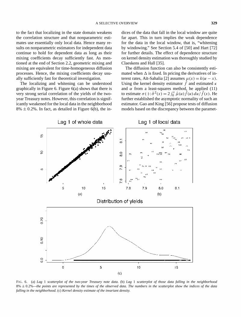
The localizing and whitening can be understoodgraphically in Figure 6. Figure 6(a) shows that there isvery strong serial correlation of the yields of the two-year Treasury notes. However, this correlation is signif-icantly weakened for the local data in the neighborhood8%± 0.2%. In fact, as detailed in Figure 6(b), the in-

dices of the data that fall in the local window are quitefar apart. This in turn implies the weak dependencefor the data in the local window, that is, “whiteningby windowing.” See Section 5.4 of [50] and Hart [72]for further details. The effect of dependence structureon kernel density estimation was thoroughly studied byClaeskens and Hall [35].

The diffusion function can also be consistently esti-mated when� is fixed. In pricing the derivatives of in-terest rates, Aït-Sahalia [2] assumesµ(x) = k(α − x).Using the kernel density estimatorf and estimatedκand α from a least-squares method, he applied (11)to estimateσ(·) : σ 2(x) = 2

∫ x0 µ(u)f (u) du/f (x). He

further established the asymptotic normality of such anestimator. Gao and King [56] propose tests of diffusionmodels based on the discrepancy between the paramet-

FIG. 6. (a) Lag 1 scatterplot of the two-year Treasury note data. (b) Lag 1 scatterplot of those data falling in the neighborhood8%± 0.2%—the points are represented by the times of the observed data. The numbers in the scatterplot show the indices of the datafalling in the neighborhood. (c) Kernel density estimate of the invariant density.

330 J. FAN

ric and nonparametric estimates of the invariant den-sity.

The Aït-Sahalia method [2] easily illustrates that thevolatility function can be consistently estimated forfixed �. However, we do not expect that it is effi-cient. Indeed, we use only the marginal information ofthe data. As shown in (21), almost all information iscontained in the transition densityp�(·|·). The tran-sition density can be estimated as in Section 4.2 be-low whether� is small or large. Since the transitiondensity and drift and volatility are in one-to-one cor-respondence for the diffusion process (5), the drift anddiffusion functions can be consistently estimated viainverting the relationship between the transition den-sity and the drift and diffusion functions.

There is no simple formula for expressing the driftand diffusion in terms of the transition density. The in-version is frequently carried out via a spectral analysisof the operatorH� = exp(�L), where the infinitesimaloperatorL is defined as

Lg(x) = σ 2(x)

2g′′(x) + µ(x)g′(x).

It has the property

Lg(x) = lim�→0

�−1[E{g(Xt+�)|Xt = x} − g(x)]by Itô’s formula (10). The operatorH� is the transitionoperator in that [see also (12)]

H�g(x) = E{g(X�)|X0 = x}.The works of Hansen and Scheinkman [66], Hansen,Scheinkman and Touzi [67] and Kessler and Sørensen[86] consist of the following idea. The first step is to es-timate the transition operatorH� from the data. Fromthe transition operator, one can identify the infinitesi-mal operatorL and hence the functionsµ(·) andσ(·).More precisely, letλ1 be the largest negative eigen-value of the operatorL with eigenfunctionξ1(x). ThenLξ1 = λ1ξ1, or equivalently,σ 2ξ ′′

1 + 2µξ ′1 = 2λ1ξ1.

This gives one equation ofµ andσ . Another equationcan be obtained via (11):(σ 2f )′ − 2µf = 0. Solvingthese two equations we obtain

σ 2(x) = 2λ1

∫ x

0ξ1(y)f (y) dy/[f (x)ξ1(x)]

and another explicit expression forµ(x). Using semi-group theory ([44], Theorem IV.3.7),ξ1 is also aneigenfunction ofH� with eigenvalue exp(�λ1). Hence,the proposal is to estimate the invariant densityf andthe transition densityp�(y|x), which implies the val-ues ofλ1 andξ1. Gobet [58] derives the optimal rate

of convergence for such a scheme, using a wavelet ba-sis. In particular, [58] shows that for fixed�, the op-timal rates of convergence forµ andσ are of ordersO(n−s/(2s+5)) andO(n−s/(2s+3)), respectively, wheres is the degree of smoothness ofµ andσ .

3.5 Time-Dependent Model

The time-dependent model (8) was introduced to ac-commodate the possibility of economic changes overtime. The coefficient functions in (8) are assumed tobe slowly time-varying and smooth. Nonparametrictechniques can be applied to estimate these coefficientfunctions. The basic idea is to localizing in time, re-sulting in a time-domain smoothing.

We first estimate the coefficient functionsα0(t)

andα1(t). For each given timet0, approximate the co-efficient functions locally by constants,α(t) ≈ a andβ(t) = b for t in a neighborhood oft0. Using the Eulerapproximation (19), we run a local regression: Mini-mize

n−1∑i=0

(Yi� − a − bXi�)2Kh(i� − t0)(27)

with respect toa and b. This results in an estimateα0(t0) = a and α1(t0) = b, where a and b are theminimizers of the local regression (27). Fan et al. [48]suggest using a one-sided kernel such asK(u) = (1−u2)I (−1 < u < 0) so that only the historical data inthe time interval(t0 − h, t0) are used in the above localregression. This facilitates forecasting and bandwidthselection. Our experience shows that there are no sig-nificant differences between nonparametric fitting withone-sided and two-sided kernels. We opt for local con-stant approximations instead of local linear approxi-mations in (27), since the local linear fit can createartificial albeit insignificant linear trends when the un-derlying functionsα0(t) and α1(t) are indeed time-independent. To appreciate this, for constant functionsα1 andα2 a large bandwidth will be chosen to reducethe variance in the estimation. This is in essence fittinga global linear regression by (27). If the local linear ap-proximations are used, since no variable selection pro-cedures have been incorporated in the local fitting (27),the slopes of the local linear approximations will not beestimated as zero and hence artificial linear trends willbe created for the estimated coefficients.

The coefficient functions in the volatility can be es-timated by the local approximated likelihood method.Let

Et = �−1/2{Xt+� − Xt − (α0(t) + α1(t)Xt

)�

}


be the normalized residuals. Then

Et ≈ β0(t)Xβ1(t)t εt .(28)

The conditional log-likelihood ofEt givenXt can eas-ily be obtained by the approximation (28). Using lo-cal constant approximations and incorporating the ker-nel weight, we obtain the local approximated likeli-hood at each time point and estimates of the functionsβ0(·) and β1(·) at that time point. This type of localapproximated-likelihood method is related to the gen-eralized method of moments of Hansen [65] and theideas of Florens-Zmirou [55] and Genon-Catalot andJacod [57].

Since the coefficient functions in both return andvolatility functions are estimated using only historicaldata, their bandwidths can be selected based on a formof the average prediction error. See Fan et al. [48] fordetails. The local least-squares regression can also beapplied to estimate the coefficient functionsβ0(t) andβ1(t) via the transformed model [see (28)]

log(E2t ) ≈ 2 logβ0(t) + β1(t) log(X2

t ) + log(ε2t ),

but we do not continue in this direction since the lo-cal least-squares estimate is known to be inefficient inthe likelihood context and the exponentiation of an es-timated coefficient function of logβ0(t) is unstable.

The question arises naturally if the coefficients inthe model (8) are really time-varying. This amounts,for example, to testingH0 :β0(t) = β0 andβ1(t) = β1.

Based on the GLR technique, Fan et al. [48] proposeda formal test for this kind of problem.

The coefficient functions in the semiparametricmodel (9) can also be estimated by using the profileapproximated-likelihood method. For each givenβ1,one can easily estimateβ0(·) via the approxima-tion (28), resulting in an estimateβ0(·;β1). Regardingthe nonparametric functionβ0(·) as being parameter-ized byβ0(·;β1), model (28) withβ1(t) ≡ β1 becomesa “synthesized” parametric model with unknownβ1.The parameterβ1 can be estimated by the maximum(approximated) likelihood method. Note thatβ1 is es-timated by using all the data points, whileβ0(t) =β0(t; β1) is obtained by using only the local datapoints. See [48] for details.

For other nonparametric methods of estimating vola-tility in time inhomogeneous models, see Härdle,Herwartz and Spokoiny [68] and Mercurio andSpokoiny [89]. Their methods are based on model (8)with α1(t) = β1(t) = 0.

3.6 State-Domain Versus Time-Domain Smoothing

So far, we have introduced both state- and time-domain smoothing. The former relies on the structuralinvariability implied by the stationarity assumption anddepends predominantly on the (remote) historical data.The latter uses the continuity of underlying parame-ters and concentrates basically on the recent data. Thisis illustrated in Figure 7 using the yields of the three-month Treasury bills from January 8, 1954 to July 16,

FIG. 7. Illustration of time- and state-domain smoothing using the yields of three-month Treasury bills. The state-domain smoothing islocalized in the horizontal bars, while the time-domain smoothing is concentrated in the vertical bars.

332 J. FAN

2004 sampled at weekly frequency. On December 28,1990, the interest rate was about 6.48%. To estimatethe drift and diffusion aroundx = 6.48, the state-domain smoothing focuses on the dynamics where in-terest rates are around 6.48%, the horizontal bar withinterest rates falling in 6.48%± 0.25%. The estimatedvolatility is basically the sample standard deviation ofthe differences{Xi� − X(i−1)�} within this horizon-tal bar. On the other hand, the time-domain smoothingfocuses predominantly on the recent history, say oneyear, as illustrated in the figure. The time-domain esti-mate of volatility is basically a sample standard devia-tion within the vertical bar.

For a given time series, it is hard to say which esti-mate is better. This depends on the underlying stochas-tic processes and also on the time when the forecast ismade. If the underlying process is continuous and sta-tionary, such as model (5), both methods are applica-ble. For example, standing at December 28, 1990, onecan forecast the volatility by using the sample standarddeviation in either the horizontal bar or the vertical bar.However, the estimated precision depends on the lo-cal data. Since the sample variance is basically linearin the squared differences{Z2

i�}, the standard errors ofboth estimates can be assessed and used to guide theforecasting.

For stationary diffusion processes, it is possible tointegrate both the time-domain and state-domain esti-mates. Note that the historical data (with interest ratesin 6.48%± 0.25%) are far apart in time from the dataused in the time-domain smoothing (vertical bar), ex-cept the last segment, which can be ignored in the state-domain fitting. The next-to-last segment with interestrates in 6.48%± 0.25% is May 11 to July 20, 1988,123 weeks prior to the last segment. Hence, these twoestimates are nearly independent. The integrated esti-mate is a linear combination of these two nearly in-dependent estimates. The weights can easily be cho-sen to minimize the variance of the integrated estima-tor, by using the assessed standard errors of the state-and time-domain estimators. The optimal weights areproportional to the variances of the two estimators,which depend on timet . This forms a dynamically inte-grated predictor for volatility estimation, as the optimalweights change over time.

3.7 Continuously Observed Data

At the theoretical level, one may also examine theproblem of estimating the drift and diffusion functionsassuming the whole process is observable up to timeT .

Let us assume again that the observed process{Xt } fol-lows the SDE (5). In this caseσ 2(Xt) is the derivativeof the quadratic variation process ofXt and hence isknown up to timeT . By (11), estimating the drift func-tion µ(x) is equivalent to estimating the invariant den-sity f . In fact,

µ(x) = [σ 2(x)f (x)]′/[2f (x)].(29)

The invariant densityf can easily be estimated bykernel density estimation. When� → 0, the summa-tion in (26) converges to

f (x) = T −1∫ T

0Kh(Xt − x)dt.(30)

This forms a kernel density estimate of the invari-ant density based on the continuously observed data.Thus, an estimator forµ(x) can be obtained bysubstituting f (x) into (29). Such an approach hasbeen employed by Kutoyants [88] and Dalalyan andKutoyants [40, 41]. They established the sharp asymp-totic minimax risk for estimating the invariant densityf and its derivative as well as the drift functionµ. Inparticular, the functionsf , f ′ andµ can be estimatedwith ratesT −1/2, T −2s/(2s+1) andT −2s/(2s+1), respec-tively, wheres is the degree of smoothness ofµ. Theseare the optimal rates of convergence.

An alternative approach is to estimate the drift func-tion directly from (23). By letting� → 0, one caneasily obtain a local linear regression estimator for con-tinuously observed data, which admits a similar formto (23) and (30). This is the approach that Spokoiny[103] used. He showed that this estimator attains theoptimal rate of convergence and established further adata-driven bandwidth such that the local linear esti-mator attains adaptive minimax rates.

4. ESTIMATION OF STATE PRICE DENSITIES ANDTRANSITION DENSITIES

The state price density (SPD) is the probability den-sity of the value of an asset under the risk-neutralworld (14) (see [38]) or equivalent martingale mea-sure [71]. It is directly related to the pricing of financialderivatives. It is the transition density ofXT givenX0under the equivalent martingaleQ. The SPD does notdepend on the payoff function and hence it can be usedto evaluate other illiquid derivatives, once it is esti-mated from more liquid derivatives. On the other hand,the transition density characterizes the probability lawof a Markovian process and hence is useful for validat-ing Markovian properties and parametric models.


4.1 Estimation of the State Price Density

For some specific models, the state price density canbe formed explicitly. For example, for the GBM (1)with a constant risk-free rater , according to (17), theSPD is log-normal with mean logx0 + (r − σ 2)/(2T )

and varianceσ 2.Assume that the SPDf ∗ exists. Then the European

call option can be expressed as

C = exp(−

∫ T

0rs ds

)∫ ∞K

(x − K)f ∗(x) dx.

See (14) (we have changed the notation fromP0 to C

to emphasize the price of the European call option).Hence,

f ∗(K) = exp(∫ T

0rs ds

)∂2C

∂K2 .(31)

This was observed by Breeden and Litzenberger [25].Thus, the state price density can be estimated from theEuropean call options with different strike prices. Withthe estimated state price density, one can price new orless liquid securities such as over-the-counter deriva-tives or nontraded options using formula (14).

In general, the price of a European call option de-pends on the current stock priceS, the strike priceK ,the time to maturityT , the risk-free interest rater anddividend yield rateδ. It can be written asC(S,K,T ,

r, δ). The exact form ofC, in general, is hard to de-termine unless we assume the Black–Scholes model.Based on historical data{(Ci, Si,Ki, Ti, ri, δi), i =1, . . . , n}, where Ci is the ith traded-option pricewith associated characteristics(Si,Ki, Ti, ri, δi), Aït-Sahalia and Lo [7] fit the nonparametric regression

Ci = C(Si,Ki, Ti, ri, δi) + εi

to obtain an estimate of the functionC and hence theSPDf ∗.

Due to the curse of dimensionality, the five-dimen-sional nonparametric function cannot be estimated wellwith practical range of sample sizes. Aït-Sahalia andLo [7] realized that and proposed a few dimensionalityreduction methods. First, by assuming that the optionprice depends only on the futures priceF = S exp((r −δ)T ), namely,

C(S,K,T , r, δ) = C(F,K,T , r)

(the Black–Scholes formula satisfies such an assump-tion), they reduced the dimensionality from five to four.By assuming further that the option-pricing function ishomogeneous of degree one inF andK , namely,

C(S,K,T , r, δ) = KC(F/K,T , r),

they reduced the dimensionality to three. Aït-Sahaliaand Lo [7] imposed a semiparametric form on the pric-ing formula,

C(S,K,T , r, δ) = CBS(F,K,T , r, σ (F,K,T )

),

whereCBS(F,K,T , r, σ ) is the Black–Scholes pricingformula given in (18) andσ(F,K,T ) is the impliedvolatility, computed by inverting the Black–Scholesformula. Thus, the problem becomes one of nonpara-metrically estimating the implied volatility functionσ(F,K,T ). This is estimated by using a nonparamet-ric regression technique from historical data, namely,

σi = σ(Fi,Ki, Ti) + εi,

whereσi is the implied volatility ofCi , by invertingthe Black–Scholes formula. By assuming further thatσ(F,K,T ) = σ(F/K,T ), the dimensionality is re-duced to two. This is one of the options in [4].

The state price densityf ∗ is nonnegative and hencethe functionC should be convex in the strike priceK .Aït-Sahalia and Duarte [6] propose to estimate the op-tion price under the convexity constraint using a locallinear estimator. See also [70] for a related approach.

4.2 Estimation of Transition Densities

The transition density of a Markov process charac-terizes the law of the process, except the initial distrib-ution. It provides useful tools for checking whether ornot such a process follows a certain SDE and for statis-tical estimation and inference. It is the state price den-sity of the price process under the risk neutral world. Ifsuch a process were observable, the state price densitywould be estimated using the methods to be introduced.

Assume that we have a sample{Xi�, i = 0, . . . , n}from model (5). The “double-kernel” method of Fan,Yao and Tong [51] is to observe that

E{Wh2(Xi� − y)|X(i−1)� = x

} ≈ p�(y|x)(32)

ash2 → 0,

for a kernel functionW . Thus, the transition densityp�(y|x) can be regarded approximately as the non-parametric regression function of the response variableWh2(Xi� − y) onX(i−1)�. An application of the locallinear estimator (23) yields

p�(y|x) =n∑

i=1

Kn

(X(i−1)� − x, x

)(33)

· Wh2(Xi� − y),

334 J. FAN

where the equivalent kernelKn(u, x) was definedin (24). Fan, Yao and Tong [51] establish the asymp-totic normality of such an estimator under stationar-ity and ρ-mixing conditions [necessarily decaying atgeometric rate for SDE (5)], which gives explicitlythe asymptotic bias and variance of the estimator. Seealso Section 6.5 of [50]. The cross-validation idea ofRudemo [98] and Bowman [24] can be extended toselect bandwidths for estimating conditional densities.See [52, 63].

The transition distribution can be estimated by in-tegrating the estimator (33) overy. By lettingh2 → 0,the estimator is the regression of the indicatorI (Xi� <

y) on X(i−1)�. Alternative estimators can be obtainedby an application of the local logistic regression andadjusted Nadaraya–Watson method of Hall et al. [64].

Early references on the estimation of the transitiondistributions and densities include [96, 97] and [95].

4.3 Inferences Based on Transition Densities

With the estimated transition density, one can nowverify whether parametric models such as (1)–(3), (6)are consistent with the observed data. Letp�,θ (y|x)

be the transition density under a parametric diffusionmodel. For example, for the CIR model (2), the pa-rameterθ = (κ,α,σ ). As in (21), ignoring the initialvalueX0, the parameterθ can be estimated by maxi-mizing

�(p�,θ ) =n∑

i=1

logp�,θ

(Xi�|X(i−1)�

).

Let θ be the maximum likelihood estimator. By thespirit of the GLR of Fan et al. [54], the GLR test forthe null hypothesisH0 :p�(y|x) = p�,θ (y|x) is

GLR= �(p�) − �(p�,θ

),

where p is a nonparametric estimate of the transi-tion density. Since the transition density cannot be es-timated well over the region where data are sparse(usually at boundaries of the process), we need totruncate the nonparametric (and simultaneously para-metric) evaluation of the likelihood at appropriate in-tervals.

In addition to employing the GLR test, one can alsocompare directly the difference between the paramet-ric and nonparametric fits, resulting in test statisticssuch as‖p� − p

�,θ‖2 and‖P� − P

�,θ‖2 for an ap-

propriate norm‖ · ‖, whereP� andP�,θ

are the esti-mates of the cumulative transition distributions underrespectively the parametric and nonparametric models.

The transition density-based methods depend on twobandwidths and are harder to implement. Indeed, theirnull distributions are harder to determine than thosebased on the transition distribution methods. In com-parison with the invariant density-based approach ofArapis and Gao [11], it is consistent against a muchlarger family of alternatives.

One can also use the transition density to testwhether an observed series is Markovian (from per-sonal communication with Yacine Aït-Sahalia). For ex-ample, if a process{Xi�} is Markovian, then

p2�(y|x) =∫ +∞−∞

p�(y|z)p�(z|x)dz.

Thus, one can use the distance betweenp2�(y|x) and∫ +∞−∞ p�(y|z)p�(z|x)dz as a test statistic.The transition density can also be used for parameter

estimation. One possible approach is to find the para-meter which minimizes the distance‖P� − P�,θ‖. Inthis case, the bandwidth should be chosen to optimizethe performance for estimatingθ . The approach is ap-plicable whether or not� → 0.

5. CONCLUDING REMARKS

Enormous efforts in financial econometrics havebeen made in modeling the dynamics of stock pricesand bond yields. There are directly related to pricingderivative securities, proprietary trading and portfo-lio management. Various parametric models have beenproposed to facilitate mathematical derivations. Theyhave risks that misspecifications of models lead to er-roneous pricing and hedging strategies. Nonparamet-ric models provide a powerful and flexible treatment.They aim at reducing modeling biases by increasingsomewhat the variances of resulting estimators. Theyprovide an elegant method for validating or suggestinga family of parametric models.

The versatility of nonparametric techniques in fi-nancial econometrics has been demonstrated in thispaper. They are applicable to various aspects of dif-fusion models: drift, diffusion, transition densities andeven state price densities. They allow us to examinewhether the stochastic dynamics for stocks and bondsare time varying and whether famous parametric mod-els are consistent with empirical financial data. Theypermit us to price illiquid or nontraded derivatives fromliquid derivatives.

The applications of nonparametric techniques in fi-nancial econometrics are far wider than what has beenpresented. There are several areas where nonparamet-ric methods have played a pivotal role. One example


is to test various versions of capital asset pricing mod-els (CAPM) and their related stochastic discount mod-els [36]. See, for example, the research manuscriptby Chen and Ludvigson [34] in this direction. An-other important class of models are stochastic volatil-ity models [19, 101], where nonparametric methodscan be also applied. The nonparametric techniqueshave been prominently featured in the RiskMetrics ofJ. P. Morgan. It can be employed to forecast the risksof portfolios. See, for example, [8, 32, 33, 47, 82] forrelated nonparametric techniques on risk management.

ACKNOWLEDGMENTS

The author gratefully acknowledges various discus-sions with Professors Yacine Aït-Sahalia and Jia-anYan and helpful comments of the editors and review-ers that led to significant improvement of the presenta-tion of this paper. This research was supported in partby NSF Grant DMS-03-55179 and a direct allocationRGC grant of the Chinese University of Hong Kong.

REFERENCES

[1] A HN, D. H. and GAO, B. (1999). A parametric nonlinearmodel of term structure dynamics.Review of Financial Stud-ies12 721–762.

[2] A ÏT-SAHALIA , Y. (1996). Nonparametric pricing of interestrate derivative securities.Econometrica64 527–560.

[3] A ÏT-SAHALIA , Y. (1996). Testing continuous-time modelsof the spot interest rate.Review of Financial Studies9 385–426.

[4] A ÏT-SAHALIA , Y. (1999). Transition densities for inter-est rate and other nonlinear diffusions.J. Finance 541361–1395.

[5] A ÏT-SAHALIA , Y. (2002). Maximum likelihood estimationof discretely sampled diffusions: A closed-form approxima-tion approach.Econometrica70 223–262.

[6] A ÏT-SAHALIA , Y. and DUARTE, J. (2003). Nonparametricoption pricing under shape restrictions.J. Econometrics1169–47.

[7] A ÏT-SAHALIA , Y. and LO, A. W. (1998). Nonparametricestimation of state-price densities implicit in financial assetprices.J. Finance53 499–547.

[8] A ÏT-SAHALIA , Y. and LO, A. W. (2000). Nonparametricrisk management and implied risk aversion.J. Econometrics94 9–51.

[9] A ÏT-SAHALIA , Y. and MYKLAND , P. (2003). The effects ofrandom and discrete sampling when estimating continuous-time diffusions.Econometrica71 483–549.

[10] AÏT-SAHALIA , Y. and MYKLAND , P. (2004). Estimatorsof diffusions with randomly spaced discrete observations:A general theory.Ann. Statist.32 2186–2222.

[11] ARAPIS, M. and GAO, J. (2004). Nonparametric kernel es-timation and testing in continuous-time financial economet-rics. Unpublished manuscript.

[12] ARFI, M. (1998). Non-parametric variance estimation fromergodic samples.Scand. J. Statist.25 225–234.

[13] BANDI , F. (2002). Short-term interest rate dynamics: A spa-tial approach.J. Financial Economics65 73–110.

[14] BANDI , F. and NGUYEN, T. (1999). Fully nonparametricestimators for diffusions: A small sample analysis. Unpub-lished manuscript.

[15] BANDI , F. and PHILLIPS, P. C. B. (2003). Fully nonpara-metric estimation of scalar diffusion models.Econometrica71 241–283.

[16] BANON, G. (1977). Estimation non paramétrique de densitéde probabilité pour les processus de Markov. Thése, Univ.Paul Sabatier de Toulouse, France.

[17] BANON, G. (1978). Nonparametric identification for diffu-sion processes.SIAM J. Control Optim.16 380–395.

[18] BANON, G. and NGUYEN, H. T. (1981). Recursive estima-tion in diffusion models.SIAM J. Control Optim.19 676–685.

[19] BARNDOFF-NIELSEN, O. E. and SHEPHARD, N. (2001).Non-Gaussian Ornstein–Uhlenbeck-based models and someof their uses in financial economics (with discussion).J. R.Stat. Soc. Ser. B Stat. Methodol.63 167–241.

[20] BINGHAM , N. H. and KIESEL, R. (1998).Risk-NeutralValuation: Pricing and Hedging of Financial Derivatives.Springer, New York.

[21] BLACK , F., DERMAN, E. and TOY, W. (1990). A one-factormodel of interest rates and its application to Treasury bondoptions.Financial Analysts Journal46(1) 33–39.

[22] BLACK , F. and KARASINSKI, P. (1991). Bond and optionpricing when short rates are lognormal.Financial AnalystsJournal47(4) 52–59.

[23] BLACK , F. and SCHOLES, M. (1973). The pricing of op-tions and corporate liabilities.J. Political Economy81 637–654.

[24] BOWMAN, A. W. (1984). An alternative method of cross-validation for the smoothing of density estimates.Bio-metrika71 353–360.

[25] BREEDEN, D. and LITZENBERGER, R. H. (1978). Prices ofstate-contingent claims implicit in option prices.J. Business51 621–651.

[26] CAI , Z., FAN, J. and YAO, Q. (2000). Functional-coefficient regression models for nonlinear time series.J.Amer. Statist. Assoc.95 941–956.

[27] CAI , Z. and HONG, Y. (2003). Nonparametric methods incontinuous-time finance: A selective review. InRecent Ad-vances and Trends in Nonparametric Statistics(M. G. Akri-tas and D. N. Politis, eds.) 283–302. North-Holland, Ams-terdam.

[28] CAMPBELL, J. Y., LO, A. W. and MACKINLAY, A. C.(1997).The Econometrics of Financial Markets. PrincetonUniv. Press.

[29] CHAN, K. C., KAROLYI , G. A., LONGSTAFF, F. A. andSANDERS, A. B. (1992). An empirical comparison of alter-native models of the short-term interest rate.J. Finance471209–1227.

[30] CHAPMAN, D. A. and PEARSON, N. D. (2000). Is the shortrate drift actually nonlinear?J. Finance55 355–388.

[31] CHEN, R. and TSAY, R. S. (1993). Functional-coefficientautoregressive models.J. Amer. Statist. Assoc.88 298–308.

336 J. FAN

[32] CHEN, S. X. (2005). Nonparametric estimation of expectedshortfall.Econometric Theory. To appear.

[33] CHEN, S. X. and TANG, C. Y. (2005). Nonparametric in-ference of value-at-risk for dependent financial returns.J.Financial Econometrics3 227–255.

[34] CHEN, X. and LUDVIGSON, S. (2003). Land of Addicts?An empirical investigation of habit-based asset pricingmodel. Unpublished manuscript.

[35] CLAESKENS, G. and HALL , P. (2002). Effect of depen-dence on stochastic measures of accuracy of density esti-mators.Ann. Statist.30 431–454.

[36] COCHRANE, J. H. (2001).Asset Pricing. Princeton Univ.Press.

[37] COX, J. C., INGERSOLL, J. E. and ROSS, S. A. (1985).A theory of the term structure of interest rates.Econometrica53 385–407.

[38] COX, J. C. and ROSS, S. (1976). The valuation of optionsfor alternative stochastic processes.J. Financial Economics3 145–166.

[39] DACUNHA-CASTELLE, D. and FLORENS, D. (1986). Esti-mation of the coefficients of a diffusion from discrete obser-vations.Stochastics19 263–284.

[40] DALALYAN , A. S. and KUTOYANTS, Y. A. (2002). Asymp-totically efficient trend coefficient estimation for ergodic dif-fusion.Math. Methods Statist.11 402–427.

[41] DALALYAN , A. S. and KUTOYANTS, Y. A. (2003). Asymp-totically efficient estimation of the derivative of the invariantdensity.Stat. Inference Stoch. Process.6 89–107.

[42] DUFFIE, D. (2001).Dynamic Asset Pricing Theory, 3rd ed.Princeton Univ. Press.

[43] EGOROV, A. V., L I , H. and XU, Y. (2003). Maximumlikelihood estimation of time-inhomogeneous diffusions.J.Econometrics114 107–139.

[44] ENGEL, K.-J. and NAGEL, R. (2000). One-ParameterSemigroups for Linear Evolution Equations. Springer,Berlin.

[45] ENGELBERT, H. J. and SCHMIDT, W. (1984). On one-dimensional stochastic differential equations with general-ized drift. Stochastic Differential Systems. Lecture Notes inControl and Inform. Sci.69 143–155. Springer, Berlin.

[46] FAN, J. (1992). Design-adaptive nonparametric regression.J. Amer. Statist. Assoc.87 998–1004.

[47] FAN, J. and GU, J. (2003). Semiparametric estimation ofvalue-at-risk.Econom. J.6 261–290.

[48] FAN, J., JIANG, J., ZHANG, C. and ZHOU, Z. (2003).Time-dependent diffusion models for term structure dynam-ics.Statist. Sinica13 965–992.

[49] FAN, J. and YAO, Q. (1998). Efficient estimation of con-ditional variance functions in stochastic regression.Bio-metrika85 645–660.

[50] FAN, J. and YAO, Q. (2003).Nonlinear Time Series: Non-parametric and Parametric Methods. Springer, New York.

[51] FAN, J., YAO, Q. and TONG, H. (1996). Estimation of con-ditional densities and sensitivity measures in nonlinear dy-namical systems.Biometrika83 189–206.

[52] FAN, J. and YIM , T. H. (2004). A crossvalidation methodfor estimating conditional densities.Biometrika91 819–834.

[53] FAN, J. and ZHANG, C. (2003). A re-examination of diffu-sion estimators with applications to financial model valida-tion. J. Amer. Statist. Assoc.98 118–134.

[54] FAN, J., ZHANG, C. and ZHANG, J. (2001). Generalizedlikelihood ratio statistics and Wilks phenomenon.Ann. Sta-tist. 29 153–193.

[55] FLORENS-ZMIROU, D. (1993). On estimating the diffusioncoefficient from discrete observations.J. Appl. Probab.30790–804.

[56] GAO, J. and KING, M. (2004). Adaptive testing incontinuous-time diffusion models.Econometric Theory20844–882.

[57] GENON-CATALOT, V. and JACOD, J. (1993). On the estima-tion of the diffusion coefficient for multi-dimensional diffu-sion processes.Ann. Inst. H. Poincaré Probab. Statist.29119–151.

[58] GOBET, E. (2002). LAN property for ergodic diffusionswith discrete observations.Ann. Inst. H. Poincaré Probab.Statist.38 711–737.

[59] GOBET, E., HOFFMANN, M. and REISS, M. (2004). Non-parametric estimation of scalar diffusions based on low fre-quency data.Ann. Statist.32 2223–2253.

[60] GOURIÉROUX, C. and JASIAK , J. (2001).Financial Econo-metrics: Problems, Models, and Methods. Princeton Univ.Press.

[61] GOURIÉROUX, C., MONFORT, A. and RENAULT, E.(1993). Indirect inference.J. Appl. Econometrics8 suppl.S85–S118.

[62] HALL , P. and CARROLL, R. J. (1989). Variance functionestimation in regression: The effect of estimating the mean.J. Roy. Statist. Soc. Ser. B51 3–14.

[63] HALL , P., RACINE, J. and LI, Q. (2004). Cross-validationand the estimation of conditional probability densities.J.Amer. Statist. Assoc.99 1015–1026.

[64] HALL , P., WOLFF, R. C. L. and YAO, Q. (1999). Methodsfor estimating a conditional distribution function.J. Amer.Statist. Assoc.94 154–163.

[65] HANSEN, L. P. (1982). Large sample properties of gen-eralized method of moments estimators.Econometrica501029–1054.

[66] HANSEN, L. P. and SCHEINKMAN , J. A. (1995). Back tothe future: Generating moment implications for continuous-time Markov processes.Econometrica63 767–804.

[67] HANSEN, L. P., SCHEINKMAN , J. A. and TOUZI, N.(1998). Spectral methods for identifying scalar diffusions.J. Econometrics86 1–32.

[68] HÄRDLE, W., HERWARTZ, H. and SPOKOINY, V. (2003).Time inhomogeneous multiple volatility modelling.J. Fi-nancial Econometrics1 55–95.

[69] HÄRDLE, W. and TSYBAKOV, A. B. (1997). Local polyno-mial estimators of the volatility function in nonparametricautoregression.J. Econometrics81 223–242.

[70] HÄRDLE, W. and YATCHEW, A. (2002). Dynamicnonparametric state price density estimation using con-strained least-squares and the bootstrap. Discussion pa-per 16, Quantification and Simulation of EconomicsProcesses, Humboldt-Universität zu Berlin.

[71] HARRISON, J. M. and KREPS, D. (1979). Martingales andarbitrage in multiperiod securities markets.J. Econom. The-ory 2 381–408.

[72] HART, J. D. (1996). Some automated methods of smoothingtime-dependent data.Nonparametr. Statist.6 115–142.


[73] HART, J. D. (1997).Nonparametric Smoothing and Lack-of-Fit Tests. Springer, New York.

[74] HASTIE, T. J. and TIBSHIRANI, R. J. (1993). Varying-coefficient models (with discussion).J. Roy. Statist. Soc. Ser.B. 55 757–796.

[75] HO, T. S. Y. and LEE, S.-B. (1986). Term structure move-ments and pricing interest rate contingent claims.J. Finance41 1011–1029.

[76] HONG, Y. and LEE, T.-H. (2003). Inference on predictabil-ity of foreign exchange rates via generalized spectrum andnonlinear time series models.Review of Economics and Sta-tistics85 1048–1062.

[77] HONG, Y. and LI, H. (2005). Nonparametric specificationtesting for continuous-time models with applications to termstructure of interest rates.Review of Financial Studies1837–84.

[78] HULL , J. (2003).Options, Futures, and Other Derivatives,5th ed. Prentice Hall, Upper Saddle River, NJ.

[79] HULL , J. and WHITE, A. (1990). Pricing interest-rate-derivative securities.Review of Financial Studies3 573–592.

[80] ITÔ, K. (1942). Differential equations determining Markovprocesses.Zenkoku Shijo Sugaku Danwakai244 1352–1400. (In Japanese.)

[81] ITÔ, K. (1946). On a stochastic integral equation.Proc.Japan Acad.22 32–35.

[82] JORION, P. (2000).Value at Risk: The New Benchmark forManaging Financial Risk, 2nd ed. McGraw–Hill, New York.

[83] KALLENBERG, O. (2002).Foundations of Modern Proba-bility, 2nd ed. Springer, New York.

[84] KARATZAS, I. and SHREVE, S. E. (1991).Brownian Mo-tion and Stochastic Calculus, 2nd ed. Springer, New York.

[85] KESSLER, M. (1997). Estimation of an ergodic diffusionfrom discrete observations.Scand. J. Statist.24 211–229.

[86] KESSLER, M. and SØRENSEN, M. (1999). Estimating equa-tions based on eigenfunctions for a discretely observed dif-fusion process.Bernoulli 5 299–314.

[87] KLOEDEN, P. E., PLATEN, E., SCHURZ, H. andSØRENSEN, M. (1996). On effects of discretization on es-timators of drift parameters for diffusion processes.J. Appl.Probab.33 1061–1076.

[88] KUTOYANTS, Y. A. (1998). Efficient density estimation forergodic diffusion processes.Stat. Inference Stoch. Process.1 131–155.

[89] MERCURIO, D. and SPOKOINY, V. (2004). Statistical infer-ence for time-inhomogeneous volatility models.Ann. Statist.32 577–602.

[90] MERTON, R. (1973). Theory of rational option pricing.BellJ. Econom. Management Sci.4 141–183.

[91] MÜLLER, H.-G. and STADTMÜLLER , U. (1987). Estima-tion of heteroscedasticity in regression analysis.Ann. Statist.15 610–625.

[92] OSBORNE, M. F. M. (1959). Brownian motion in the stockmarket.Operations Res.7 145–173.

[93] PHAM , D. T. (1981). Nonparametric estimation of the driftcoefficient in the diffusion equation.Math. Operations-forsch. Statist. Ser. Statist.12 61–73.

[94] PRAKASA RAO, B. L. S. (1985). Estimation of the drift fordiffusion process.Statistics16 263–275.

[95] ROSENBLATT, M. (1970). Density estimates and Markovsequences. InNonparametric Techniques in Statistical In-ference(M. L. Puri, ed.) 199–213. Cambridge Univ. Press.

[96] ROUSSAS, G. G. (1969). Nonparametric estimation inMarkov processes.Ann. Inst. Statist. Math.21 73–87.

[97] ROUSSAS, G. G. (1969). Nonparametric estimation of thetransition distribution function of a Markov process.Ann.Math. Statist.40 1386–1400.

[98] RUDEMO, M. (1982). Empirical choice of histograms andkernel density estimators.Scand. J. Statist.9 65–78.

[99] RUPPERT, D., WAND, M. P., HOLST, U. and HÖSSJER,O. (1997). Local polynomial variance function estimation.Technometrics39 262–273.

[100] SCHURZ, H. (2000). Numerical analysis of stochastic dif-ferential equations without tears. InHandbook of StochasticAnalysis and Applications(D. Kannan and V. Lakshmikan-tham, eds.) 237–359. Dekker, New York.

[101] SHEPHARD, N., ed. (2005).Stochastic Volatility: SelectedReadings. Oxford Univ. Press.

[102] SIMONOFF, J. S. (1996).Smoothing Methods in Statistics.Springer, New York.

[103] SPOKOINY, V. (2000). Adaptive drift estimation for non-parametric diffusion model.Ann. Statist.28 815–836.

[104] STANTON, R. (1997). A nonparametric model of term struc-ture dynamics and the market price of interest rate risk.J.Finance52 1973–2002.

[105] STEELE, J. M. (2001).Stochastic Calculus and FinancialApplications. Springer, New York.

[106] VASICEK, O. A. (1977). An equilibrium characterization ofthe term structure.J. Financial Economics5 177–188.

[107] WAND, M. P. and JONES, M. C. (1995).Kernel Smoothing.Chapman and Hall, London.

[108] WANG, Y. (2002). Asymptotic nonequivalence of GARCHmodels and diffusions.Ann. Statist.30 754–783.

[109] YOSHIDA, N. (1992). Estimation for diffusion processesfrom discrete observations.J. Multivariate Anal. 41220–242.


Comment: A Selective Overview ofNonparametric Methods inFinancial EconometricsPeter C. B. Phillips and Jun Yu

Abstract. These comments concentrate on two issues arising from Fan’soverview. The first concerns the importance of finite sample estimation biasrelative to the specification and discretization biases that are emphasized inFan’s discussion. Past research and simulations given here both reveal thatfinite sample effects can be more important than the other two effects whenjudged from either statistical or economic viewpoints. Second, we draw at-tention to a very different nonparametric technique that is based on comput-ing an empirical version of the quadratic variation process. This technique isnot mentioned by Fan but has many advantages and has accordingly attractedmuch recent attention in financial econometrics and empirical applications.

Key words and phrases: Nonparametric method, continuous time models,financial time series, jackknife, realized volatility.

1. INTRODUCTION

In recent years there has been increased interest inusing nonparametric methods to deal with various as-pects of financial data. The paper by Fan gives anoverview of some nonparametric techniques that havebeen used in the financial econometric literature, focus-ing on estimation and inference for diffusion models incontinuous time and estimation of state price and tran-sition density functions.

Continuous time specifications have been heavilyused in recent work, partly because of the analyticconvenience of stochastic calculus in mathematical fi-nance and partly because of the availability of high-frequency data sets for many financial series. Whilethe early work in continuous-time finance began inthe 1970s with the work of Merton [29] and Blackand Scholes [16], economists have been looking at the

Peter C. B. Phillips is Professor, Cowles Founda-tion for Research in Economics, Yale University, Box208281, New Haven, Connecticut 06520-8281, USA(e-mail: [email protected]). Jun Yu is AssociateProfessor, School of Economics and Social Science,Singapore Management University, 90 Stamford Road,Singapore 178903 (e-mail: [email protected]).

econometric problems of fitting continuous time sys-tems for much longer. The idea of statistically fittingdiffusion models and continuously distributed laggeddependencies with discretely observed data has a longhistory dating back to some original work in econo-metrics by Koopmans [27] and subsequent work byPhillips [31], Bergstrom [14], Sims [35], Phillips [32]and Sargan [34]. Bartlett and Rajalakshman [13] andBartlett [12] are two references in the early statisticalliterature on fitting linear diffusions. Bergstrom [15]provides a short history of some of this early work.Also, the history of mathematical finance and sto-chastic integration prior to 1970 has recently beenoverviewed in an interesting historical review by Jarrowand Protter [24].

Our comments on Fan’s paper will concentrate ontwo issues that relate in important ways to the paper’sfocus on misspecification and discretization bias andthe role of nonparametric methods in empirical finance.The first issue deals with the finite sample effects ofvarious estimation methods and their implications forasset pricing. A good deal of recent attention in theeconometric literature has focused on the benefits offull maximum likelihood (ML) estimation of diffusionsand mechanisms for avoiding discretization bias in theconstruction of the likelihood. However, many of the

338

A SELECTIVE OVERWIEV 339

problems of estimating dynamic models that are wellknown in discrete time series, such as the bias in MLestimation, also manifest in the estimation of contin-uous time systems and affect subsequent use of theseestimates, for instance in derivative pricing. In conse-quence, a relevant concern is the relative importanceof the estimation and discretization biases. As we willshow below, the former often dominates the latter evenwhen the sample size is large (at least 500 monthly ob-servations, say). Moreover, it turns out that correctionfor the finite sample estimation bias continues to bemore important when the diffusion component of themodel is itself misspecified. Such corrections appearto be particularly important in models that are nonsta-tionary or nearly nonstationary.

The second issue we discuss deals with a very differ-ent nonparametric technique, which is not discussed byFan, but which has recently attracted much attention infinancial econometrics and empirical applications. Thismethod involves the use of quadratic variation mea-sures of realized volatility using ultra high frequencyfinancial data. Like other nonparametric methods, em-pirical quadratic variation techniques also have to dealwith statistical bias, which in the present case arisesfrom the presence of microstructure noise. The field ofresearch on this topic in econometrics is now very ac-tive.

2. FINITE SAMPLE EFFECTS

In his overview of diffusion equation estimation, Fandiscusses two sources of bias, one arising from the dis-cretization process and the second from misspecifica-tion. We review these two bias effects and then discussthe bias that comes from finite sample estimation ef-fects.

The attractions of Itô calculus have made it partic-ularly easy to work with stochastic differential equa-tions driven by Brownian motion. Diffusion processesin particular have been used widely in finance to modelasset prices, including stock prices, interest rates andexchange rates. Despite their mathematical attractabil-ity, diffusion processes present some formidable chal-lenges for econometric estimation. The primary reasonfor the difficulty is that sample data, even very high-frequency data, are always discrete and for many popu-lar nonlinear diffusion models the transition density ofthe discrete sample does not have a closed form expres-sion, as noted by Fan. The problem is specific to non-linear diffusions, as consistent methods for estimatingexact discrete models corresponding to linear systems

of diffusions have been available since Phillips [32].A simple approach discussed in the paper is to use theEuler approximation scheme to discretize the model,a process which naturally creates some discretizationbias. This discretization bias can lead to erroneousfinancial pricing and investment decisions. In conse-quence, the issue of discretization has attracted a lot ofattention in the literature and many methods have beenproposed to reduce the bias that it causes. Examples arePedersen [30], Kessler [26], Durham and Gallant [18],Aït-Sahalia [2, 3] and Elerian, Chib and Shephard [19],among many others.

Next, many diffusion models in practical use arespecified in a way that makes them mathematicallyconvenient. These specifications are typically not de-rived from any underlying economic theory and aretherefore likely to be misspecified. Potential misspec-ifications, like discretization, can lead to erroneous fi-nancial decisions. Accordingly, specification bias hasattracted a great deal of attention in the literature andhas helped to motivate the use of functional estimationtechniques that treat the drift and diffusion coefficientsnonparametrically. Important contributions includeAït-Sahalia [1], Stanton [36], Bandi and Phillips [5]and Hong and Li [21].

While we agree that both discretization and specifi-cation bias are important issues, finite sample estima-tion bias can be of equal or even greater importance forfinancial decision making, as noted by Phillips and Yu[33] in the context of pricing bonds and bond options.The strong effect of the finite sample estimation bias inthis context can be explained as follows. In continuoustime specifications, the prices of bonds and bond op-tions depend crucially on the mean reversion parameterin the associated interest rate diffusion equation. Thisparameter is well known to be subject to estimationbias when standard methods like ML are used. The biasis comparable to, but generally has larger magnitudethan, the usual bias that appears in time series autore-gression. As the parameter is often very close to zeroin empirical applications (corresponding to near mar-tingale behavior and an autoregressive root near unityin discrete time), the estimation bias can be substantialeven in very large samples.

To reduce the finite sample estimation bias in para-meter estimation as well as the consequential bias thatarises in asset pricing, Phillips and Yu [33] proposedthe use of jackknife techniques. Suppose a sample ofn

observations is available and that this sample is decom-posed intom consecutive sub-samples each with� ob-servations (n = m × �). The jackknife estimator of a

340 P. C. B. PHILLIPS AND J. YU

parameterθ in the model is defined by

θjack = m

m − 1θn −

∑mi=1 θ�i

m2 − m,(2.1)

whereθn and θ�i are the extreme estimates ofθ basedon the entire sample and thei ’th sub-sample, respec-tively. The parameterθ can be a coefficient in the dif-fusion process, such as the mean reversion parameter,or a much more complex function of the parametersof the diffusion process and the data, such as an assetprice or derivative price. Typically, the full sample ex-treme estimator has bias of orderO(n−1), whereas un-der mild conditions the bias in the jackknife estimate isof orderO(n−2).

The following simulation illustrates these variousbias effects and compares their magnitudes. In the ex-periment, the true generating process is assumed to bethe following commonly used model (CIR hereafter)of short term interest rates due to Cox, Ingersoll andRoss [17]:

dr(t) = κ(µ − r(t)

)dt + σr1/2(t) dB(t).(2.2)

The transition density of the CIR model is known tobece−u−v(v/u)q/2Iq(2(uv)1/2) and the marginal den-sity isw

w21 rw2−1e−w1r/�(w2), wherec = 2κ/(σ 2(1−

e−κ�)), u = cr(t)e−κ�, v = cr(t + �), q = 2κµ/

σ 2−1, w1 = 2κ/σ 2, w2 = 2κµ/σ 2, � is the samplingfrequency, andIq(·) is the modified Bessel function ofthe first kind of orderq. The transition density togetherwith the marginal density can be used for simulationpurposes as well as to obtain the exact ML estimator ofθ (= (κ,µ,σ )′). In the simulation, we use this modelto price a discount bond, which is a three-year bondwith a face value of $1 and initial interest rate of 5%,and a one-year European call option on a three-yeardiscount bond which has a face value of $100 and astrike price of $87. The reader is referred to [33] forfurther details.

In addition to exact ML estimation, we may dis-cretize the CIR model via the Euler method and es-timate the discretized model using (quasi-) ML. TheEuler scheme leads to the discretization

r(t + �) = κµ� + (1− κ�)r(t)

+ σN(0,�r(t)

).

(2.3)

One thousand samples, each with 600 monthly ob-servations (i.e.,� = 1/12), are simulated from thetrue model (2.2) with(κ,µ,σ )′ being set at(0.1,0.08,0.02)′, which are settings that are realistic in manyfinancial applications. To investigate the effects of

discretization bias, we estimate model (2.3) by the(quasi-) ML approach. To investigate the finite sampleestimation bias effects, we estimate model (2.2) basedon the true transition density. To examine the effectsof bias reduction in estimation, we apply the jackknifemethod (withm = 3) to the mean reversion parame-ter κ , the bond price and the bond option price.

To examine the effects of specification bias, we fiteach simulated sequence from the true model to themisspecified Vasicek model [37] to obtain the exactML estimates ofκ , the bond price and the option pricefrom this misspecified model. The Vasicek model isgiven by the simple linear diffusion

dr(t) = κ(µ − r(t)

)dt + σ dB(t).(2.4)

We use this model to price the same bond and bondoption. Vasicek [37] derived the expression for bondprices and Jamshidian [23] gave the corresponding for-mula for bond option prices. The transition density forthe Vasicek model is

r(t + �)|r(t)∼ N

(µ(1− e−κ�)

+ e−κ�rt , σ2(1− e−2κ�)/(2κ)

).

(2.5)

This transition density is utilized to obtain the exactML estimates ofκ , the bond price and the bond op-tion price, all under the mistaken presumption that themisspecified model (2.4) is correctly specified.

Table 1 reports the means and root mean square er-rors (RMSEs) for all these cases. It is clear that thefinite sample estimation bias is more substantial than

TABLE 1Finite sample properties of ML and jackknife estimates of κ , bondprice and option price for the (true) CIR model using a (correctly

specified ) fitted CIR model and a (misspecified ) fitted Vasicekmodel (sample size n = 600)

Parameter κ Bond price Option price

True value 0.1 0.8503 2.3920

Exact ML Mean 0.1845 0.8438 1.8085of CIR RMSE 0.1319 0.0103 0.9052Euler ML Mean 0.1905 0.8433 1.7693of CIR RMSE 0.1397 0.0111 0.9668Jackknife (m = 3) Mean 0.0911 0.8488 2.1473of CIR RMSE 0.1205 0.0094 0.8704ML of Vasicek Mean 0.1746 0.8444 1.8837(misspecified) RMSE 0.1175 0.0088 0.7637Jackknife (m = 2) of Mean 0.0977 0.8488 2.2483Vasicek (misspecified) RMSE 0.1628 0.0120 1.0289


the discretization bias and the specification bias for allthree quantities, at least in this experiment. In particu-lar, κ is estimated by the exact ML method with 84.5%upward bias, which contributes toward the−0.76%bias in the bond price and the−24.39% bias in theoption price. Relative to the finite sample bias, thebias in κ due to the discretization is almost negli-gible since the total bias inκ changes from 84.5%to 90.5%. (The increase in the total bias indicatesthat the discretization bias effect is in the same di-rection as that of the estimation bias.) The total biaschanges from−0.76% to −0.82% in the bond priceand from−24.39% to −26.03% in the option price.These changes are marginal. Similarly, relative to thefinite sample bias, the bias inκ due to misspecificationof the drift function is almost negligible since the totalbias changes from 84.5% to 74.6%. (The decrease inthe total bias indicates that the misspecification bias ef-fect is in the opposite direction to that of the estimationbias.) The total bias changes from−0.76% to−0.69%in the bond price and from−24.39% to−21.25% inthe option price. Once again, these changes are mar-ginal. When the jackknife method is applied to the cor-rectly specified model, the estimation bias is greatlyreduced in all cases (from 84.5% to−8.9% for κ ;from −0.76% to −0.18% for the bond price; andfrom −24.39% to−10.23% for the option price).

Even more remarkably, when the jackknife methodis applied to the incorrectly specified model (see the fi-nal row of Table 1), the estimation bias is also greatlyreduced in all cases (from 84.5% to−2.3% for κ ;from −0.76% to −0.18% for the bond price; andfrom −24.39% to−6.01% for the option price). Thesefigures reveal that dealing with estimation bias can bemuch more important than ensuring correct specifica-tion in diffusion equation estimation, suggesting thatgeneral econometric treatment of the diffusion throughnonparametric methods may not address the majorsource of bias effects on financial decision making.

Although the estimation bias is not completely re-moved by the jackknife method, the bias reduction isclearly substantial and the RMSE of the jackknife es-timate is smaller in all cases than that of exact ML. Insum, it is apparent from Table 1 that the finite sampleestimation bias is larger in magnitude than either of thebiases due to discretization and misspecification andcorrecting this bias is therefore a matter of importancein empirical work on which financial decisions depend.

Although this demonstration of the relative impor-tance of finite sample estimation bias in relation to dis-cretization bias and specification bias is conducted in

a parametric context, similar results can be expectedfor some nonparametric models. For example, in thesemiparametric model examined in [1], the diffusionfunction is nonparametrically specified and the driftfunction is linear, so that the mean reversion parameteris estimated parametrically as in the above example. Insuch cases, we can expect substantial finite sample es-timation bias to persist and to have important practicalimplications in financial pricing applications.

3. REALIZED VOLATILITY

As noted in Fan’s overview, many models used in fi-nancial econometrics for modeling asset prices and in-terest rates have the fully functional scalar differentialform

dXt = µ(Xt) dt + σ(Xt) dBt ,(3.1)

where both drift and diffusion functions are nonpara-metric and where the equation is driven by Brownianmotion incrementsdBt . For models such as (3.1), wehave(dXt)

2 = σ 2(Xt) dt a.s. and hence the quadraticvariation ofXt is

[X]T =∫ T

0(dXt)

2 dt =∫ T

0σ 2(Xt) dt,(3.2)

where∫ T0 σ 2(Xt) dt is the accumulated or integrated

volatility of X. WereXt observed continuously,[X]Tand, hence, integrated volatility, would also be ob-served. For discretely recorded data, estimation of (3.2)is an important practical problem. This can be accom-plished by direct nonparametric methods using an em-pirical estimate of the quadratic variation that is calledrealized volatility. The idea has been discussed forsome time, an early reference being Maheswaran andSims [28], and it has recently attracted a good deal ofattention in the econometric literature now that veryhigh frequency data has become available for empiricaluse. Recent contributions to the subject are reviewed in[4] and [8].

SupposeXt is recorded discretely at equispacedpoints(�,2�, . . . , n��(≡ T )) over the time interval[0, T ]. Then,[X]T can be consistently estimated by therealized volatility ofXt defined by

[X�]T =n�∑i=2

(Xi� − X(i−1)�

)2,(3.3)

as� → 0, as is well known. In fact, any constructionof realized volatility based on an empirical grid of ob-servations where the maximum grid size tends to zerowill produce a consistent estimate. It follows that the

342 P. C. B. PHILLIPS AND J. YU

integrated volatility can be consistently estimated bythis nonparametric approach, regardless of the form ofµ(Xt) andσ(Xt). The approach has received a greatdeal of attention in the recent volatility literature andserves as a powerful alternative to the methods dis-cussed by Fan, especially when ultra-high frequencydata are available.

While this approach is seemingly straightforward,it is not without difficulties. First, in order for theapproach to be useful in empirical research, it isnecessary to estimate the precision of the realizedvolatility estimates. Important contributions on thecentral limit theory of these empirical quadratic vari-ation estimates by Jacod [22] and Barndorff-Nielsonand Shephard [10, 11] has facilitated the constructionof suitable methods of inference. Second, in practicalapplications, realized volatility measures such as (3.3)are usually contaminated by microstructure noise bias,especially at ultra high frequencies and tick-by-tickdata. Noise sources arise from various market frictionsand discontinuities in trading behavior that prevent thefull operation of efficient financial markets. Recentwork on this subject (e.g., [8, 9, 21, 38]) has devel-oped various methods, including nonparametric kerneltechniques, for reducing the effects of microstructurenoise bias.

4. ADDITIONAL ISSUES

Given efficient market theory, there is good reason toexpect that diffusion models like (3.1) may have non-stationary characteristics. Similar comments apply toterm structure models and yield curves. In such cases,nonparametric estimation methods lead to the estima-tion of the local time (or sojourn time) of the cor-responding stochastic process and functionals of thisquantity, rather than a stationary probability density.Moreover, rates of convergence in such cases becomepath dependent and the limit theory for nonparametricestimates of the drift and diffusion functions in (3.1)is mixed normal. Asymptotics of this type require anenlarging time span of data as well as increasing in-fillwithin each discrete interval asn → ∞. An overviewof this literature and its implications for financial dataapplications is given in [6]. Nonparametric estimatesof yield curves in multifactor term structure models arestudied in [25].

Not all models in finance are driven by Brown-ian motion. In some cases, one can expect noise tohave to have some memory and, accordingly, models

such as (3.1) have now been extended to accommo-date fractional Brownian motion increments. The sto-chastic calculus of fractional Brownian motion, whichis not a semi-martingale, is not as friendly as that ofBrownian motion and requires new constructs, involv-ing Wick products and versions of the Stratonovich in-tegral. Moreover, certain quantities, such as quadraticvariation, that have proved useful in the recent empiri-cal literature may no longer exist and must be replacedby different forms of variation, although the idea ofvolatility is still present. Developing a statistical theoryof inference to address these issues in financial econo-metric models is presenting new challenges.

ACKNOWLEDGMENTS

Peter C. B. Phillips gratefully acknowledges visit-ing support from the School of Economics and SocialScience at Singapore Management University. Sup-port was provided by NSF Grant SES-04-142254. JunYu gratefully acknowledges financial support from theWharton-SMU Research Center at Singapore Manage-ment University.

REFERENCES

[1] A ÏT-SAHALIA , Y. (1996). Nonparametric pricing of interestrate derivative securities.Econometrica 64 527–560.

[2] A ÏT-SAHALIA , Y. (1999). Transition densities for interestrate and other nonlinear diffusions.J. Finance 54 1361–1395.

[3] A ÏT-SAHALIA , Y. (2002). Maximum likelihood estimation ofdiscretely sampled diffusions: A closed-form approximationapproach.Econometrica 70 223–262.

[4] A NDERSEN, T. G., BOLLERSLEV, T. and DIEBOLD, F. X.(2005). Parametric and nonparametric volatility measure-ment. InHandbook of Financial Econometrics (Y. Aït-Sahaliaand L. P. Hansen, eds.). North-Holland, Amsterdam. To ap-pear.

[5] BANDI , F. M. and PHILLIPS, P. C. B. (2003). Fully nonpara-metric estimation of scalar diffusion models.Econometrica71 241–283.

[6] BANDI , F. M. and PHILLIPS, P. C. B. (2005). Nonstation-ary continuous-time processes. InHandbook of FinancialEconometrics (Y. Aït-Sahalia and L. P. Hansen, eds.). North-Holland, Amsterdam. To appear.

[7] BANDI , F. M. and RUSSELL, J. (2005). Volatility. InHand-book of Financial Engineering (J. R. Birge and V. Linetsky,eds.). To appear.

[8] BANDI , F. M. and RUSSELL, J. (2005). Microstructure noise,realized volatility and optimal sampling. Working paper,Graduate School of Business, Univ. Chicago.

[9] BARNDORFF-NIELSEN, O., HANSEN, P., LUNDE, A. andSHEPHARD, N. (2005). Regular and modified kernel-basedestimators of integrated variance: The case with independentnoise. Working paper, Nuffield College.


[10] BARNDORFF-NIELSEN, O. and SHEPHARD, N. (2002).Econometric analysis of realized volatility and its use in esti-mating stochastic volatility models.J. R. Stat. Soc. Ser. B Stat.Methodol. 64 253–280.

[11] BARNDORFF-NIELSEN, O. and SHEPHARD, N. (2004).Econometric analysis of realized covariation: High frequencybased covariance, regression, and correlation in financial eco-nomics.Econometrica 72 885–925.

[12] BARTLETT, M. S. (1955). An Introduction to StochasticProcesses. Cambridge Univ. Press.

[13] BARTLETT, M. S. and RAJALAKSHMAN , D. V. (1953).Goodness of fit tests for simultaneous autoregressive series.J. Roy. Statist. Soc. Ser. B 15 107–124.

[14] BERGSTROM, A. (1966). Nonrecursive models as discreteapproximations to systems of stochastic differential equa-tions.Econometrica 34 173–182.

[15] BERGSTROM, A. (1988). The history of continuous-timeeconometric models.Econometric Theory 4 365–383.

[16] BLACK , F. and SCHOLES, M. (1973). The pricing of optionsand corporate liabilities.J. Political Economy 81 637–654.

[17] COX, J., INGERSOLL, J. and ROSS, S. (1985). A theory ofthe term structure of interest rates.Econometrica 53 385–407.

[18] DURHAM, G. and GALLANT , A. R. (2002). Numerical tech-niques for maximum likelihood estimation of continuous-time diffusion processes (with discussion).J. Bus. Econom.Statist. 20 297–338.

[19] ELERIAN, O., CHIB, S. and SHEPHARD, N. (2001). Likeli-hood inference for discretely observed non-linear diffusions.Econometrica 69 959–993.

[20] HANSEN, P. and LUNDE, A. (2006). An unbiased measureof realized volatility.J. Bus. Econom. Statist. To appear.

[21] HONG, Y. and LI, H. (2005). Nonparametric specificationtesting for continuous-time models with applications to termstructure of interest rates.Review of Financial Studies 1837–84.

[22] JACOD, J. (1994). Limit of random measures associated withthe increments of a Brownian semimartingale. Working pa-per, Univ. P. and M. Curie, Paris.

[23] JAMSHIDIAN , F. (1989). An exact bond option formula.J. Fi-nance 44 205–209.

[24] JARROW, R. and PROTTER, P. (2004). A short history of sto-chastic integration and mathematical finance: The early years,

1880–1970. InA Festschrift for Herman Rubin (A. DasGupta,ed.) 75–91. IMS, Beachwood, OH.

[25] JEFFREY, A., KRISTENSEN, D., LINTON, O., NGUYEN, T.and PHILLIPS, P. C. B. (2004). Nonparametric estimation ofa multifactor Heath–Jarrow–Morton model: An integrated ap-proach.J. Financial Econometrics 2 251–289.

[26] KESSLER, M. (1997). Estimation of an ergodic diffusionfrom discrete observations.Scand. J. Statist. 24 211–229.

[27] KOOPMANS, T., ed. (1950).Statistical Inference in DynamicEconomic Models. Wiley, New York.

[28] MAHESWARAN, S. and SIMS, C. A. (1993). Empirical im-plications of arbitrage-free asset markets. InModels, Meth-ods and Applications of Econometrics (P. C. B. Phillips, ed.)301–316. Blackwell, Cambridge, MA.

[29] MERTON, R. (1973). Theory of rational option pricing.BellJ. Econom. and Management Sci. 4 141–183.

[30] PEDERSEN, A. (1995). A new approach to maximum likeli-hood estimation for stochastic differential equations based ondiscrete observations.Scand. J. Statist. 22 55–71.

[31] PHILLIPS, A. W. (1959). The estimation of parameters insystems of stochastic differential equations.Biometrika 4667–76.

[32] PHILLIPS, P. C. B. (1972). The structural estimation ofa stochastic differential equation system.Econometrica 401021–1041.

[33] PHILLIPS, P. C. B. and YU, J. (2005). Jackknifing bond op-tion prices.Review of Financial Studies 18 707–742.

[34] SARGAN, J. D. (1974). Some discrete approximations to con-tinuous time stochastic models.J. Roy. Statist. Soc. Ser. B 3674–90.

[35] SIMS, C. (1971). Discrete approximations to continuous timedistributed lags in econometrics.Econometrica 39 545–563.

[36] STANTON, R. (1997). A nonparametric model of term struc-ture dynamics and the market price of interest rate risk.J. Fi-nance 52 1973–2002.

[37] VASICEK, O. (1977). An equilibrium characterization of theterm structure.J. Financial Economics 5 177–188.

[38] ZHANG, L., MYKLAND , P. and AÏT-SAHALIA , Y. (2005).A tale of two time scales: Determining integrated volatilitywith noisy high-frequency data.J. Amer. Statist. Assoc. 1001394–1411.


Comment: A Selective Overview ofNonparametric Methods inFinancial EconometricsMichael Sørensen

1. INTRODUCTION

Professor Fan should be congratulated for his reviewthat convincingly demonstrates the usefulness of non-parametric techniques to financial econometric prob-lems. He is mainly concerned with financial modelsgiven by stochastic differential equations, that is, dif-fusion processes. I will therefore complement his se-lective review by discussing some important problemsand useful methods for diffusion models that he hasnot covered. My concern will mainly, but not solely, bewith parametric techniques. A recent comprehensivesurvey of parametric inference for discretely sampleddiffusion models can be found in [19].

2. GAUSSIAN LIKELIHOOD FUNCTIONS

In his brief review of parametric methods, Profes-sor Fan mentions the Gaussian approximate likelihoodfunction based on the Euler scheme and states that thismethod has some bias when the time between observa-tions� is large. This is actually a very serious problem.As an example, consider a model with a linear drift ofthe formµ(x) = −β(x − α) (β > 0). The estimatorβn

of β obtained from the Gaussian approximate likeli-hood based on the Euler scheme converges to

(1− e−β0�)�−1

as the number of observationsn tends to infinity.Hereβ0 denotes the true parameter value. The limitingvalue of�βn is always smaller than one, and the limitof βn is always smaller than�−1. Thus the asymp-totic bias can be huge if� is large. A simulation studyin [3] demonstrates that also for finite sample sizes anenormous bias can occur. When�β0 is small so that(1 − e−β0�)�−1 ≈ β0, the asymptotic bias is negligi-ble. The problem is, however, that if we use the approx-imate likelihood function based on the Euler scheme,

Michael Sørensen is Professor and Head, Departmentof Applied Mathematics and Statistics, University ofCopenhagen, Universitetsparken 5, DK-2100 Copen-hagen Ø, Denmark (e-mail: [email protected]).

there is no way we can know whether�β0 is smallor large because�βn will always tend to be small.I suspect that the nonparametric methods outlined inSections 3.2 and 3.5 might suffer from a similar short-coming as they are based on the same type of approxi-mation as the Euler scheme.

A simple solution to this problem is to use an ap-proximate likelihood function where the transition den-sity is replaced by a normal distribution with meanequal to the exact conditional expectationF(x, θ) =Eθ(X�|X0 = x) and with the variance equal to the ex-act conditional variance�(x; θ) = Varθ (X�|X0 = x).Here θ is the (typically multivariate) parameter tobe estimated. This approach is exactly the same asusing quadratic martingale estimating functions; see[3] and [20]. The estimators obtained from quadraticmartingale estimating functions have the same niceproperties for high frequency observations (small�) asthe estimators based on the Euler likelihood, but theyare consistent for any value of� and can thus be usedwhether or not� is small. In most cases there is no ex-plicit expression for the functionsF(x, θ) and�(x; θ),so often they must be determined by simulation. Thisrequires, however, only a modest amount of computa-tion and is not a problem in practice. If a completelyexplicit likelihood is preferred, one can approximateF(x, θ) and�(x; θ) by expansions of a higher orderthan those used in the Euler scheme; see [16].

The nonparametric method in Section 3.5 couldprobably be improved in a similar way by using in(27) and (28) the functionsF(x, θ) and �(x; θ) (orthe higher-order expansions in [16]) instead of the first-order approximation used in the Euler scheme.

3. MARTINGALE ESTIMATING FUNCTIONS

More generally, martingale estimating functions pro-vide a simple and versatile technique for estimationin discretely sampled parametric stochastic differentialequation models that works whether or not� is small.

344


An estimator is obtained by solving the equationn∑

i=1

N∑j=1

aj

(X(i−1)�; θ)

· [fj (Xi�) − Hθ

�fj

(X(i−1)�

)] = 0,

where H� is the transition operator, and where thefunction a has the same dimension as the parameterθ . First suitable functionsfj are chosen, and then theweight functionsaj are determined so that an opti-mal estimating function in the sense of Godambe andHeyde [9] is obtained; see also [10]. Optimal estimat-ing functions are approximations to the non-explicitscore function. UsuallyHθ

�fj must be determinedby a modest amount of simulation, but Kessler andSørensen [17] demonstrated how completely explicitestimating functions can be obtained if the functionsfj

are eigenfunctions of the operatorLθ (called the gener-ator); see also [18] for details on how to explicitly findthe optimal weight functions. A review of the theory ofestimating functions for discretely sampled diffusion-type models can be found in [1].

For martingale estimating functions large sampleresults concerning estimators can be obtained via mar-tingale limit theory. Under weak conditions, estima-tors are consistent, and optimal estimating functionstend to work well when the functionsfj are chosenreasonably, that is, such that a good approximation tothe score function can be obtained. At low samplingfrequencies the estimators are, however, usually notefficient. The behavior of the estimators at high sam-pling frequencies can be investigated by consideringan asymptotic scenario where the time between ob-servations�n is assumed to go to zero, as the sam-ple sizen tends to infinity, sufficiently slowly that thetime horizon over which observations are made,n�n,tends to infinity. It is well known that in this situationestimators of parameters appearing in the diffusion co-efficient may converge at a suboptimal rate, 1/

√n�n.

The reason is that there is a lot of information about thediffusion coefficient in the fine structure of diffusiontrajectories, which some estimators do not capture.Recently Sørensen [22] has given conditions ensuringthat a martingale estimating function provides estima-tors that are rate-optimal (rate 1/

√n ) and efficient in

the high-frequency asymptotic scenario. Optimal mar-tingale estimating functions satisfy these conditions.Quadratic martingale estimating functions are alwaysrate-optimal, and if they are obtained from Gaussianapproximate likelihood functions they are efficient too.These results are closely related to the theory of small�-optimality developed in [13] and [14].

4. NON-MARKOVIAN OBSERVATIONS

There are several situations in which observationsfrom a diffusion process are non-Markovian. Mostprominently this happens if a function of lower di-mension of a multivariate diffusion is observed. Anexample is the stochastic volatility model that plays animportant role as a model of financial time series sinceit is well known that a simple one-dimensional diffu-sion often cannot capture all the salient features of suchdata. Another example is given by the sums of diffu-sions proposed by Bibby, Skovgaard and Sørensen [2]as models of phenomena with more than one timescale. Other situations where diffusion data are non-Markovian are in the presence of measurement error, orwhen only integrals of the diffusion over time-intervalsare observed; see [4]. The latter is, for instance, thecase when climate data from ice cores are analyzed bymeans of a diffusion model. When the data are non-Markovian, it is usually not possible to find a tractablemartingale estimating function, but an alternative isprovided by the prediction-based estimating functionsproposed in [21], which can be interpreted as approxi-mations to martingale estimating functions.

Asymptotic results for estimators based on non-Markovian data are usually based on the assump-tion that the underlying diffusion process is stronglymixing. The condition ensuring exponentialρ-mixingcited in Section 2.2 is not easy to check for concretediffusion models. A condition on the drift and diffusioncoefficient that is easy to verify and that implies expo-nentialρ-mixing andα-mixing was given by Genon-Catalot, Jeantheau and Larédo [6].

5. NONPARAMETRIC METHODS

Let me conclude by drawing attention to some rel-atively early work on nonparametric methods for dis-cretely sampled diffusion models. Wavelet methods forestimating the diffusion coefficient of a time-dependentmodel were proposed by Genon-Catalot, Larédo andPicard [7]. The first estimator of the diffusion coef-ficient mentioned in Section 3.2 was first proposedby Florens-Zmirou [5]. She considered a high fre-quency asymptotic scenario with fixed time span, thatis, with n�n constant, and proved that the asymptoticdistribution of her estimator is a mixture of normaldistributions where the mixing distribution is the dis-tribution of the local time of the diffusion. If a data-dependent normalization of the estimator is used, anasymptotic normal distribution is obtained. In a series

346 M. SØRENSEN

of important papers, Marc Hoffmann has studied opti-mal rates of convergence of nonparametric estimatorsof the drift and diffusion coefficient under the threeasymptotic scenarios usually considered for diffusionmodels including optimal estimators; see [8, 11, 12].Other estimators of the diffusion coefficient were pro-posed by Soulier [23] and Jacod [15].

REFERENCES

[1] BIBBY, B. M., JACOBSEN, M. and SØRENSEN, M. (2005).Estimating functions for discretely sampled diffusion-typemodels. InHandbook of Financial Econometrics (Y. Aït-Sahalia and L. P. Hansen, eds.). North-Holland, Amsterdam.To appear.

[2] BIBBY, B. M., SKOVGAARD, I. M. and SØRENSEN, M.(2005). Diffusion-type models with given marginal distribu-tion and autocorrelation function.Bernoulli 11 191–220.

[3] BIBBY, B. M. and SØRENSEN, M. (1995). Martingale esti-mation functions for discretely observed diffusion processes.Bernoulli 1 17–39.

[4] DITLEVSEN, S. and SØRENSEN, M. (2004). Inference forobservations of integrated diffusion processes.Scand. J. Sta-tist. 31 417–429.

[5] FLORENS-ZMIROU, D. (1993). On estimating the diffusioncoefficient from discrete observations.J. Appl. Probab. 30790–804.

[6] GENON-CATALOT, V., JEANTHEAU, T. and LARÉDO, C.(2000). Stochastic volatility models as hidden Markov mod-els and statistical applications.Bernoulli 6 1051–1079.

[7] GENON-CATALOT, V., LARÉDO, C. and PICARD, D.(1992). Nonparametric estimation of the diffusion coefficientby wavelet methods.Scand. J. Statist. 19 317–335.

[8] GOBET, E., HOFFMANN, M. and REISS, M. (2004). Non-parametric estimation of scalar diffusions based on low fre-quency data.Ann. Statist. 32 2223–2253.

[9] GODAMBE, V. P. and HEYDE, C. C. (1987). Quasi-likelihood and optimal estimation.Internat. Statist. Rev. 55231–244.

[10] HEYDE, C. C. (1997).Quasi-Likelihood and Its Application.Springer, New York.

[11] HOFFMANN, M. (1999). Adaptive estimation in diffusionprocesses.Stochastic Process. Appl. 79 135–163.

[12] HOFFMANN, M. (1999).Lp estimation of the diffusion coef-ficient.Bernoulli 5 447–481.

[13] JACOBSEN, M. (2001). Discretely observed diffusions:Classes of estimating functions and small�-optimality.Scand. J. Statist. 28 123–149.

[14] JACOBSEN, M. (2002). Optimality and small�-optimality ofmartingale estimating functions.Bernoulli 8 643–668.

[15] JACOD, J. (2000). Nonparametric kernel estimation of the co-efficient of a diffusion.Scand. J. Statist. 27 83–96.

[16] KESSLER, M. (1997). Estimation of an ergodic diffusionfrom discrete observations.Scand. J. Statist. 24 211–229.

[17] KESSLER, M. and SØRENSEN, M. (1999). Estimating equa-tions based on eigenfunctions for a discretely observed diffu-sion process.Bernoulli 5 299–314.

[18] LARSEN, K. S. and SØRENSEN, M. (2005). A diffusionmodel for exchange rates in a target zone.Math. Finance.To appear.

[19] SØRENSEN, H. (2004). Parametric inference for diffusionprocesses observed at discrete points in time: A survey.In-ternat. Statist. Rev. 72 337–354.

[20] SØRENSEN, M. (1997). Estimating functions for discretelyobserved diffusions: A review. In Selected Proceedingsof the Symposium on Estimating Functions (I. V. Basawa,V. P. Godambe and R. L. Taylor, eds.) 305–325. IMS, Hay-ward, CA.

[21] SØRENSEN, M. (2000). Prediction-based estimating func-tions.Econom. J. 3 123–147.

[22] SØRENSEN, M. (2005). Efficient martingale estimating func-tions for discretely sampled ergodic diffusions. Preprint,Dept. Appl. Math. and Statistics, Univ. Copenhagen.

[23] SOULIER, P. (1998). Nonparametric estimation of the diffu-sion coefficient of a diffusion process.Stochastic Anal. Appl.16 185–200.


Comment: A Selective Overview ofNonparametric Methods inFinancial EconometricsPer A. Mykland and Lan Zhang

We would like to congratulate Jianqing Fan for anexcellent and well-written survey of some of the lit-erature in this area. We will here focus on some ofthe issues which are at the research frontiers in finan-cial econometrics but are not covered in the survey.Most importantly, we consider the estimation of actualvolatility. Related to this is the realization that financialdata is actually observed with error (typically calledmarket microstructure), and that one needs to considera hidden semimartingale model. This has implicationsfor the Markov models discussed above.

For reasons of space, we have not included refer-ences to all the relevant work by the authors that arecited, but we have tried to include at least one refer-ence to each of the main contributors to the realizedvolatility area.

1. THE ESTIMATION OF ACTUAL VOLATILITY:THE IDEAL CASE

The paper discusses the estimation of Markoviansystems, models where the drift and volatility coeffi-cients are functions of timet or statex. There is, how-ever, scope for considering more complicated systems.An important tool in this respect is the direct estima-tion of volatility based on high-frequency data. Oneconsiders a system of, say, log securities prices, whichfollows:

dXt = µt dt + σt dBt ,(1)

whereBt is a standard Brownian motion. Typically,µt ,the drift coefficient, andσ 2

t , the instantaneous variance

Per A. Mykland is Professor, Department of Statis-tics, The University of Chicago, Chicago, Illinois60637, USA (e-mail: [email protected]).Lan Zhang is Assistant Professor, Department of Fi-nance, University of Illinois at Chicago, Chicago, Illi-nois 60607, and Department of Statistics, CarnegieMellon University, Pittsburgh, Pennsylvania 15213,USA (e-mail: [email protected]).

(or volatility) of the returns processXt , will be sto-chastic processes, but these processes can depend onthe past in ways that need not be specified, and can besubstantially more complex than a Markov model. Thisis known as anItô process.

A main quantity of econometric interest is to obtain

time series of the form�i = ∫ T +i

T −i

σ 2t dt , i = 1,2, . . . .

HereT −i andT +

i can, for example, be the beginningand the end of day numberi. �i is variously knownas theintegrated variance (or volatility) or quadraticvariation of the processX. The reason why one canhope to obtain this series is as follows. IfT −

i = t0 <

t1 < · · · < tn = T +i spans day numberi, define there-

alized volatility by

�i =n−1∑j=0

(Xtj+1 − Xtj

)2.(2)

Then stochastic calculus tells us that

�i = limmax|tj+1−tj |→0

�i .(3)

In the presence of high frequency financial data, inmany cases with transactions as often as every few sec-onds, one can, therefore, hope to almostobserve �i .One can then either fit a model to the series of�i , orone can use it directly for portfolio management (asin [12]), options hedging (as in [29]), or to test good-ness of fit [31].

There are too many references to the relationship (3)to name them all, but some excellent treatments canbe found in [27], Section 1.5; [26], Theorem I.4.47on page 52; and [33], Theorem II-22 on page 66. Anearly econometric discussion of this relationship canbe found in [2].

To make it even more intriguing, recent work bothfrom the probabilistic and econometric sides givesthe mixed normal distribution of the error in the ap-proximation in (3). References include [6, 25, 31].

The random variance of the normal error is 2T +

i −T −i

n·

347

348 P. A. MYKLAND AND L. ZHANG

∫ T +i

T −i

σ 4t dH(t), whereH is thequadratic variation of

time. H(t) = t in the case where theti are equidistant.Further econometric literature includes, in particu-

lar, [3, 4, 8, 9, 14, 18, 32]. Problems that are attached tothe estimation of covariations between two processesare discussed in [22]. Estimatingσ 2

t at each pointtgoes back to [13]; see also [30], but this has not caughton quite as much in econometric applications.

2. THE PRESENCE OF MEASUREMENT ERROR

The theory described above runs into a problem withreal data. For illustration, consider how the realizedvolatility depends on sampling frequency for the stock(and day) considered in Figure 1. The estimator doesnot converge as the observation pointsti become densein the interval of this one day, but rather seems to takeoff to infinity. This phenomenon was originally docu-mented in [2]. For transaction data, this picture is re-peated for most liquid securities [19, 37].

In other words, the model (1) is wrong. What can onedo about this? A lot of people immediately think that

the problem is due to jumps, but that is not the case.The limit in (3) exists even when there are jumps. Therequirement for (3) to exist is that the processX be asemimartingale (we again cite Theorem I.4.47 of [26]),which includes both Itô processes and jumps.

The inconsistency between the empirical resultswhere the realized volatility diverges with finer sam-pling, and the semimartingale theory which dictatesthe convergence of the realized volatility, poses a prob-lem, since financial processes are usually assumedto be semimartingales. Otherwise, somewhat looselyspeaking, there would be arbitrage opportunities inthe financial markets. For rigorous statements, see, inparticular, [11]. The semimartingaleness of financialprocesses, therefore, is almost a matter of theology inmost of finance, and yet, because of Figure 1 and sim-ilar graphs for other stocks, we have to abandon it.

Our alternative model is that there is measurementerror in the observation. At transaction numberi, in-stead of seeingXti from model (1) or, more generally,from a semimartingale, one observes

Yti = Xti + εi.(4)

FIG. 1. Plot of realized volatility for Alcoa Aluminum for January 4, 2001. The data is from the TAQ database. There are 2011 trans-actions on that day, on average one every 13.365seconds. The most frequently sampled volatility uses all the data, and this is denoted as“ frequency = 1.” “ Frequency = 2” corresponds to taking every second sampling point. Because this gives rise to two estimators of volatility,we have averaged the two. And so on for “ frequency = k” up to 20.The plot corresponds to the average realized volatility discussed in [37].Volatilities are given on an annualized and square root scale.


We call this thehidden semimartingale model. The ra-tionale is (depending on your subject matter) eitherthat a transaction is a measurement of the underlyingpriceXti , and of course there is error, or that it is due tomarket microstructure, as documented by, among oth-ers, Roll [34], Glosten [15], Glosten and Harris [16],Brown [7], Harris [20] and Hasbrouck [21]. See [1] fora discussion of this.

A natural model for the error is that it is either i.i.d.or a stationary process, as considered by Zhou [38],Gloter and Jacod [17], Zhang, Mykland and Aït-Sahalia [37], Bandi and Russell [5], Zhang [36],Aït-Sahalia, Mykland and Zhang [1] and Hansen andLunde [19].

Under quite loose conditions, this alternative modelis consistent with the plot in Figure 1. Instead of (3),one gets that the realized volatility becomesnE(ε1 −ε0)

2 + Op(n−1/2). In the early literature (as cited inthe previous section), the problem is usually taken careof by (sic) reducingn. A variety of approaches thatimprove on this are documented in [37], to which werefer for an in depth discussion. As demonstrated byZhang [36], the true volatility�i can be consistentlyestimated at rateOp(n−1/4), as opposed toOp(n−1/2)

when there is no error. This is not as slow as it seems,sincen is quite large for liquid securities.

An alternative description of the error is that it arisesdue to rounding (financial instruments are, after all,traded on a price grid). Research in this direction hasbeen done by Delattre and Jacod [10] and by Zeng [35].To first order, the rounding and additive error modelsare similar, as documented by Delattre and Jacod [10];see also [28].

It is awkward that these models imply the existenceof arbitrage. The size of the error, however, is so smallthat it is hard to take economic advantage of them, andthis, presumably, is why such deviations can persist.

3. IMPLICATIONS FOR MARKOV MODELS

We now return to the subject to Jianqing Fan’soverview, namely the Markov case. It is clear that themodel without observation error is not consistent withthe data. This may not be a problem when workingwith, say, daily data, but would pose problems whenusing high-frequency (intraday) observations. It is pre-sumably quite straightforward to extend the methodsdiscussed in the paper to the case of observation er-ror, and it would be interesting to see the results. Thesame applies to similar studies on Markov modelsby the “French school,” such as Hoffmann [23] andJacod [24].

ACKNOWLEDGMENT

We gratefully acknowledge the support of the Na-tional Science Foundation under Grant DMS-02-04639.

REFERENCES

[1] A ÏT-SAHALIA , Y., MYKLAND , P. A. and ZHANG, L.(2005). How often to sample a continuous-time process in thepresence of market microstructure noise.Review of FinancialStudies 18 351–416.

[2] A NDERSEN, T. G., BOLLERSLEV, T., DIEBOLD, F. X. andLABYS, P. (2000). Great realizations.Risk 13 105–108.

[3] A NDERSEN, T. G., BOLLERSLEV, T., DIEBOLD, F. X. andLABYS, P. (2001). The distribution of realized exchange ratevolatility. J. Amer. Statist. Assoc. 96 42–55.

[4] A NDERSEN, T. G., BOLLERSLEV, T., DIEBOLD, F. X. andLABYS, P. (2003). Modeling and forecasting realized volatil-ity. Econometrica 71 579–625.

[5] BANDI , F. M. and RUSSELL, J. R. (2005). Microstructurenoise, realized volatility and optimal sampling. Technical re-port, Graduate School of Business, Univ. Chicago.

[6] BARNDORFF-NIELSEN, O. E. and SHEPHARD, N. (2002).Econometric analysis of realized volatility and its use in esti-mating stochastic volatility models.J. R. Stat. Soc. Ser. B Stat.Methodol. 64 253–280.

[7] BROWN, S. J. (1990). Estimating volatility. InFinancialOptions: From Theory to Practice (S. Figlewski, W. Silberand M. Subrahmanyam, eds.) 516–537. Business One-Irwin,Homewood, IL.

[8] CHERNOV, M. and GHYSELS, E. (2000). A study towards aunified approach to the joint estimation of objective and riskneutral measures for the purpose of options valuation.J. Fi-nancial Economics 56 407–458.

[9] DACOROGNA, M. M., GENÇAY, R., MÜLLER, U., OLSEN,R. B. and PICTET, O. V. (2001).An Introduction to High-Frequency Finance. Academic Press, San Diego.

[10] DELATTRE, S. and JACOD, J. (1997). A central limit theo-rem for normalized functions of the increments of a diffusionprocess, in the presence of round-off errors.Bernoulli 3 1–28.

[11] DELBAEN, F. and SCHACHERMAYER, W. (1995). The ex-istence of absolutely continuous local martingale measures.Ann. Appl. Probab. 5 926–945.

[12] FLEMING, J., KIRBY, C. and OSTDIEK, B. (2001). The eco-nomic value of volatility timing.J. Finance 56 329–352.

[13] FOSTER, D. and NELSON, D. (1996). Continuous record as-ymptotics for rolling sample variance estimators.Economet-rica 64 139–174.

[14] GALLANT , A. R., HSU, C.-T. and TAUCHEN, G. (1999). Us-ing daily range data to calibrate volatility diffusions and ex-tract the forward integrated variance.Review of Economicsand Statistics 81 617–631.

[15] GLOSTEN, L. R. (1987). Components of the bid-ask spreadand the statistical properties of transaction prices.J. Finance42 1293–1307.

[16] GLOSTEN, L. R. and HARRIS, L. E. (1988). Estimating thecomponents of the bid/ask spread.J. Financial Economics 21123–142.

350 P. A. MYKLAND AND L. ZHANG

[17] GLOTER, A. and JACOD, J. (2000). Diffusions with measure-ment errors: I—Local asymptotic normality and II—Optimalestimators. Technical report, Univ. de Paris VI.

[18] GONCALVES, S. and MEDDAHI, N. (2005). Bootstrappingrealized volatility. Technical report, Univ. de Montréal.

[19] HANSEN, P. R. and LUNDE, A. (2006). Realized varianceand market microstructure noise.J. Bus. Econom. Statist.To appear.

[20] HARRIS, L. (1990). Statistical properties of the Roll serialcovariance bid/ask spread estimator.J. Finance 45 579–590.

[21] HASBROUCK, J. (1993). Assessing the quality of a securitymarket: A new approach to transaction-cost measurement.Review of Financial Studies 6 191–212.

[22] HAYASHI , T. and YOSHIDA, N. (2005). On covariance es-timation of non-synchronously observed diffusion processes.Bernoulli 11 359–379.

[23] HOFFMANN, M. (1999).Lp estimation of the diffusion coef-ficient.Bernoulli 5 447–481.

[24] JACOD, J. (2000). Nonparametric kernel estimation of the co-efficient of a diffusion.Scand. J. Statist. 27 83–96.

[25] JACOD, J. and PROTTER, P. (1998). Asymptotic error distri-butions for the Euler method for stochastic differential equa-tions.Ann. Probab. 26 267–307.

[26] JACOD, J. and SHIRYAEV, A. N. (2003).Limit Theorems forStochastic Processes, 2nd ed. Springer, New York.

[27] KARATZAS, I. and SHREVE, S. E. (1991).Brownian Motionand Stochastic Calculus, 2nd ed. Springer, New York.

[28] KOLASSA, J. and MCCULLAGH , P. (1990). Edgeworth seriesfor lattice distributions.Ann. Statist. 18 981–985.

[29] MYKLAND , P. A. (2003). Financial options and statisticalprediction initervals.Ann. Statist. 31 1413–1438.

[30] MYKLAND , P. A. and ZHANG, L. (2001). Inference forvolatility type objects and implications for hedging. Technicalreport, Dept. Statistics, Carnegie Mellon Univ.

[31] MYKLAND , P. A. and ZHANG, L. (2002). ANOVA for diffu-sions. Technical report, Dept. Statistics, Univ. Chicago.

[32] OOMEN, R. (2004). Properties of realized variance for a purejump process: Calendar time sampling versus business timesampling. Technical report, Warwick Business School, Univ.Warwick.

[33] PROTTER, P. (2004).Stochastic Integration and DifferentialEquations: A New Approach, 2nd ed. Springer, New York.

[34] ROLL, R. (1984). A simple implicit measure of the effec-tive bid-ask spread in an efficient market.J. Finance 391127–1139.

[35] ZENG, Y. (2003). A partially-observed model for micro-movement of asset process with Bayes estimation via filter-ing. Math. Finance 13 411–444.

[36] ZHANG, L. (2004). Efficient estimation of stochastic volatil-ity using noisy observations: A multi-scale approach. Techni-cal report, Dept. Statistics, Carnegie Mellon Univ.

[37] ZHANG, L., MYKLAND , P. A. and AÏT-SAHALIA , Y.(2005). A tale of two time scales: Determining integratedvolatility with noisy high-frequency data.J. Amer. Statist. As-soc. 100 1394–1411.

[38] ZHOU, B. (1996). High-frequency data and volatility inforeign-exchange rates.J. Bus. Econom. Statist. 14 45–52.


Rejoinder: A Selective Overview ofNonparametric Methods inFinancial EconometricsJianqing Fan

I am very grateful to the Executive Editor, EdwardGeorge, for organizing this stimulating discussion.I would like to take this opportunity to thank Pro-fessors Peter Phillips, Jun Yu, Michael Sørensen, PerMykland and Lan Zhang for their insightful and stimu-lating comments, touching both practical, methodolog-ical and theoretical aspects of financial econometricsand their applications in asset pricing, portfolio alloca-tion and risk management. They have made valuablecontributions to the understanding of various financialeconometric problems.

The last two decades have witnessed an explosionof developments of data-analytic techniques in statis-tical modeling and analysis of complex systems. Atthe same time, statistical techniques have been widelyemployed to confront various complex problems aris-ing from financial and economic activities. While thediscipline has grown rapidly over the last two decadesand has rich and challenging statistical problems, thenumber of statisticians involved in studying financialeconometric problems is still limited. In comparisonwith statisticians working on problems in biologicalsciences and medicine, the group working on finan-cial and econometric problems is dismally small. It ismy hope that this article will provide statisticians withquick access to some important and interesting prob-lems in financial econometrics and to catalyze the ro-mance between statistics and finance. A similar effortwas made by Cai and Hong [12], where various aspectsof nonparametric methods in continuous-time financeare reviewed. It is my intention to connect financialeconometric problems as closely to statistical problemsas possible so that familiar statistical tools can be em-ployed. With this in mind, I sometimes oversimplifythe problems and techniques so that key features canbe highlighted.

Jianqing Fan is Professor, Benheim Center of Financeand Department of Operations Research and FinancialEngineering, Princeton University, Princeton, NewJersey 08544, USA (e-mail: [email protected]).

I am fully aware that financial econometrics hasgrown into a vast discipline itself and that it is im-possible for me to provide an overview within a rea-sonable length. Therefore, I greatly appreciate whatall discussants have done to expand the scope of dis-cussion and provide additional references. They havealso posed open statistical problems for handling non-stationary and/or non-Markovian data with or withoutmarket noise. In addition, statistical issues on variousversions of capital asset pricing models and their re-lated stochastic discount models [15, 19], the efficientmarket hypothesis [44] and risk management [17, 45]have barely been discussed. These reflect the vibrantintersection of the interfaces between statistics and fi-nance. I will make some further efforts in outliningeconometric problems where statistics plays an impor-tant role after brief response to the issues raised by thediscussants.

1. BIASES IN STATISTICAL ESTIMATION

The contributions by Professors Phillips, Yu andSørensen address the bias issues on the estimation ofparameters in diffusion processes. Professors Phillipsand Yu further translate the bias of diffusion parame-ter estimation into those of pricing errors of bonds andbond derivatives. Their results are very illuminatingand illustrate the importance of estimation bias in fi-nancial asset pricing. Their results can be understoodas follows. Suppose that the price of a financial assetdepends on certain parametersθ (the speed of the re-versionκ in their illustrative example). Let us denote itby p(θ), which can be in one case the price of a bondand in another case the prices of derivatives of a bond.The value of the asset is now estimated byp(θ) with θ

being estimated from empirical data. Whenθ is overes-timated (say), which shifts the whole distribution ofθ

to the left, the distribution ofp(θ) will also be shifted,depending on the sensitivity ofp to θ . The sensitivityis much larger for bond derivatives whenκ is close tozero (see Figure 2 of [46]), and hence the pricing errorsare much larger. On the other hand, as the distribution

351

352 J. FAN

of κ is shifted to the left, from Figure 2 of [46], bothprices of bonds and their derivatives get smaller and sodoes the variance of pricing errors. Simulation studiesin [46] suggest that these two effects cancel each otherout in terms of mean square error.

I agree with Phillips and Yu’s observation that dis-cretization is not the main source of biases for manyreasonable financial applications. Finite-sample esti-mation bias can be more severe. This partially an-swers the question raised by Professor Sørensen. Onthe other hand, his comments give theoretical insightsinto the bias due to discretization. For financial ap-plications (such as modeling short-term rates) whenthe data are collected at monthly frequency, the bias{1−exp(−κ�)}/�−κ = −0.0019 and−0.00042, re-spectively, forκ = 0.21459 used in Figure 3 of [34] andfor κ = 0.1 used in the discussion by Phillips and Yu.For weekly data, using the parameterκ = 0.0446 citedin [14], the discretization bias is merely 9.2× 10−5.

For other types of applications, such as climatol-ogy, Professor Sørensen is right that the bias due todiscretization can sometimes be substantial. It is boththeoretically elegant and practically viable to havemethods that work well for all situations. The quasi-maximum likelihood methods and their modificationsdiscussed by Professor Sørensen are attractive alter-natives. As he pointed out, analytical solutions arerare and computation algorithms are required. This in-creases the chance of numerical instability in practi-cal implementations. The problem can be attenuatedwith the estimates based on the Euler approximationas an initial value. The martingale method is a gener-alization of his quasi-maximum likelihood estimator,which aims at improving efficiency by suitable choiceof weighting functionsaj . However, unless the con-ditional density has multiplicative score functions, theestimation equations will not be efficient. This explainsthe observation made by Professor Sørensen that themethods based on martingale estimating functions areusually not efficient for low frequency data. The abovediscussion tends to suggest that when the Euler approx-imation is reasonable, the resulting estimates tend tohave smaller variances.

In addition to the discretization bias and finite sam-ple estimation bias, there is model specification bias.This can be serious in many applications. In the ex-ample given by Professors Phillips and Yu, the mod-eling errors do not have any serious adverse effectson pricing bonds and their derivatives. However, weshould be wary of generalizing this statement. Indeed,for the model parameters given in the discussion by

Phillips and Yu, the transition density of the CIR modelhas a noncentralχ2-distributions with degrees of free-dom 80, which is close to the normal transition densitygiven by the Vasicek model. Therefore, the model isnot very seriously misspecified.

Nonparametric methods reduce model specificationerrors by either global modeling such as spline meth-ods or local approximations. This reduces significantlythe possibility of specification errors. Since nonpara-metric methods are somewhat crude and often usedas model diagnostic and exploration tools, simple andquick methods serve many practical purposes. For ex-ample, in time domain smoothing, the bandwidthh isalways an order of magnitude larger than the samplingfrequency�. Therefore, the approximation errors dueto discretization are really negligible. Similarly, formany realistic problems, the function approximationerrors can be an order of magnitude larger than dis-cretization errors. Hence, discretization errors are oftennot a main source of errors in nonparametric inference.

2. HIGH-FREQUENCY DATA

Professors Mykland, Zhang, Phillips and Jun addressstatistical issues for high-frequency data. I greatlyappreciate their insightful comments and their elabora-tions on the importance and applications of the subject.Thanks to the advances in modern trading technology,the availability of high-frequency data over the lastdecade has significantly increased. Research in thisarea has advanced very rapidly lately. I would like tothank Professors Mykland and Zhang for their compre-hensive overview on this active research area.

With high-frequency data, discretization errors havesignificantly been reduced. Nonparametric methodsbecome even more important for this type of largesample problem. The connections between the realizedvolatility and the time-inhomogeneous model can sim-ply be made as follows. Consider a subfamily of mod-els of (8) in [34],

dXt = αt dt + σt dWt .

For high-frequency data the sampling interval is verysmall. For the sampling frequency of a minute,� =1/(252∗ 24 ∗ 60) ≈ 2.756× 10−6. Hence, standard-ized residuals in Section 2.5 of [34] becomeEt =�−1/2(Xt+� − Xt) and the local constant estimate ofthe spot volatility reduces to

σ 2j� =

j−1∑i=−∞

wj−iE2i�,


where{wi} are the weights induced by a kernel func-tion satisfying

∑∞i=1 wi = 1. Now, for the weights

with a bounded support, the quadratic variation of theprocess or integrated volatility

∫ Tt σ 2

t dt is naturally es-

timated by�∑T/�−1

i=t/� σ 2i , which is simply

T/�−1∑i=t/�

{Xi� − X(i−1)�

}2.

This shows that our nonparametric estimation of theintegrated volatility for high-frequency data is indeedthe same as the realized volatility.

As suggested by Professors Mykland, Zhang,Phillips and Yu, the applications of realized volatili-ties are not without difficulties. Market microstructurenoises emerge at such a fine frequency of observationand market prices can contain multiple jumps dueto the flux of information during a trading session.Figure 1 in the discussion by Mykland and Zhangdemonstrates convincingly the existence of the mar-ket microstructure noise. Aït-Sahalia, Mykland andZhang [1] and Zhang, Mykland and Aït-Sahalia [50]give comprehensive accounts of this under the assump-tion that the observed prices are the true ones conta-minated with random noise of market microstructure:Yt = Xt + εt . However, they do not take into accountthat the price processes{Xt } may contain jumps inaddition to random noises. An effort in this directionhas been made recently by Fan and Wang [38] usingwavelet techniques.

3. ESTIMATING COVARIANCE MATRICES

Covariance matrices play an important role in riskmanagement and asset allocation. They are featuredprominently in many financial econometrics problems.For example, the smallest and largest eigenvalues arerelated to the minimum and the maximum of thevolatility of portfolios and their corresponding eigen-vectors are related to portfolio allocation. See [40] forapplications of covariance matrices to portfolio selec-tion and [43] for their applications to other scientificproblems. There are a couple of approaches to thesekinds of problems, depending on the size of the co-variance matrices. I hereby give a brief overview andaddress some of the open challenges.

The simplest estimate of a covariance matrix is prob-ably the sample covariance matrix of the log-returnsof p assets over a period ofn days prior to the currenttime t . This is indeed a nonparametric estimation ofthe covariance matrix localizing in time and has been

studied in multivariate analysis whenp is finite andthe underlying model is correct, that is, the covariancematrix remains the same in then days prior to timet .See, for example, [26, 27, 47]. However, the impact ofthe biases in nonparametric methods on the estimationof eigenvalues and eigenvectors has not yet been thor-oughly investigated.

The sample covariance matrices can be augmentedby using the information from the state domain, whichis an extension of the method discussed in Section 3.6of [34] and allows us to use the historical information.This is particularly useful for estimating the covari-ance matrices of bonds with different maturities. Use-ful parametric models such as affine models have beenpopularly used in interest rate modeling. See, for exam-ple, [20, 24, 23]. Nonparametric methods provide use-ful alternatives to estimating the covariance matricesand to validating parametric models. A naive extensioninvolves high-dimensional smoothing in the state do-main. But this can be avoided by localizing only on theyields of a few bonds with intermediate length of ma-turity.

Another class of techniques is to use a form ofGARCH model [28] to estimate covariance matri-ces. As noted in [30], the number of parametersgrows rapidly with the dimensionalityp. Various ef-forts have been made to reduce the complexity ofthe models. These include constant conditional cor-relation multivariate GARCH models [10], vectorizedmultivariate GARCH models [11], dynamic condi-tional correlation models [29, 31], orthogonal GARCHmodels [2], generalized orthogonal GARCH mod-els [48] and conditionally uncorrelated componentmodels [37]. For a survey, see [8].

In portfolio allocation and risk management, thenumber of stocksp can be well in the order of hun-dreds, which is typically in the same order as the sam-ple sizen. The sample covariance matrix may not be agood estimator of the population one. The estimatedvariance of a portfolio based on the sample covari-ance may far exceed the true one. The estimation errorscan accumulate quickly whenp grows withn. Indeed,Johnstone [43] shows that the largest eigenvalue of thecovariance matrix is far larger than the population one.There are many studies on the behavior of random ma-trices when the dimensionalityp grows with n. See,for example, [5, 22, 21, 49]. For a survey, see [4].

Estimating covariance matrices for largep is in-trinsically challenging. For example, whenp = 200,there are more than 20,000 free parameters. Yet, the

354 J. FAN

available sample size is usually in the order of hun-dreds or a few thousand. Longer time series (largern)will increase modeling biases. Without imposing struc-tures on the covariance matrices, they are hard to esti-mate. Thanks to the multi-factor models (see Chapter 6of [13]), if a few factors can capture completely thecross-sectional risks, the number of parameters can besignificantly reduced. For example, using the Fama–French three-factor models [32, 33], there are 4p in-stead ofp(p+1)/2 parameters. Natural questions arisewith this structured estimate of the covariance matrix,how largep can be such that the estimation error in thecovariance matrix is negligible in asset allocation andrisk management. The problems of this kind are inter-esting and remain open.

Another possible approach to the estimation of co-variance matrices is to use a model selection ap-proach. First of all, according to Chapter 3 of [39],the Cholesky decomposition admits nice autoregres-sive interpretation. We may reasonably assume that theelements in the Cholesky decomposition of the covari-ance matrix are sparse. Hence, the penalized likelihoodmethod [3, 35, 42] can be employed to select and es-timate nonsparse elements. The sampling property ofsuch a method remains unknown. Its impact on portfo-lio allocation and risk management needs to be studied.

4. STATISTICS IN DERIVATIVE PRICING

Over last three decades, option pricing has witnessedan explosion of new models that extend the originalwork of Black and Scholes [9]. Empirically pricing fi-nancial derivatives is innately related to statistical re-gression problems. This is well documented in paperssuch as [6, 7, 15, 16, 25, 41]. See also a brief reviewgiven by Cai and Hong [12]. For a given stochasticmodel with given structural parameters under the risk-neutral measure, the prices of European options canbe determined, which are simply the discounted ex-pected payoffs under the risk-neutral measure. Bakshi,Cao and Chen [6] give the analytic formulas of op-tion prices for five commonly used stochastic mod-els, including the stochastic-volatility random-jumpmodel. They then estimate the risk-neutral parame-ters by minimizing the discrepancies between the ob-served prices and the theoretical ones. With estimatedrisk-neutral parameters, option prices with differentcharacteristics can be evaluated. They conduct a com-prehensive study of the relative merits of competingoption pricing models by computing pricing errors fornew options. Dumas, Fleming and Whaley [25] model

the implied volatility function by a quadratic func-tion of the strike price and time to maturity and deter-mine these parameters by minimizing pricing errors.Based on the analytic formula of Bakshi, Cao andChen [6] for option price under the stochastic volatil-ity models, Chernov and Ghysels [16] estimate therisk neutral parameters by integrating information fromboth historical data and risk-neutral data implied byobserved option prices. Instead of using continuous-time diffusion models, Heston and Nandi [41] assumethat the stock prices under the risk-neutral world fol-low a GARCH model and derive a closed form forEuropean options. They determine the structural pa-rameters by minimizing the discrepancy between theempirical and theoretical option prices. Barone-Adesi,Engle and Mancini [7] estimate risk-neutral parame-ters by integrating the information from both historicaldata and option prices. Christoffersen and Jakobs [18]expand the flexility of the model by introducing long-and short-run volatility components.

The above approaches can be summarized as fol-lows. Using the notation in Section 4.1 of [34], thetheoretical option price with option characteristics(Si,Ki, Ti, ri, δi) is governed by a parametric formC(Si,Ki, Ti, ri, δi, θ), whereθ is a vector of structuralparameters of the stock price dynamics under the risk-neutral measure. The form depends on the underlyingparameters of the stochastic model. This can be in onecase a stochastic volatility model and in another casea GARCH model. The parameters are then determinedby minimizing

n∑i=1

{Ci − C(Si,Ki, Ti, ri, δi, θ)}2

or similar discrepancy measures. The success of amethod depends critically on the correctness of modelassumptions under the risk-neutral measure. Sincethese assumptions are not on the physical measure,they are hard to verify. This is why so many para-metric models have been introduced. Their efforts canbe regarded as searching an appropriate parametricform C(·; θ) to better fit the option data. Nonparamet-ric methods in Section 4.1 provide a viable alternativefor this purpose. They can be combined with paramet-ric approaches to improve the accuracy of pricing.

As an illustration, let us consider the options withfixed (Si, Ti, ri, δi) so that their prices are only a func-tion of K or equivalently a function of the moneynessm = K/S,

C = exp(−rT )

∫ ∞K

(x − K)f ∗(x) dx.


(a) (b)

FIG. 1. (a) Scatterplot of the response variable computed based on option prices with consecutive strike price against the moneyness.(b) The implied volatilities of the options during the period July 7–11, 2003.

DenotingD = exp(rT )C/S and lettingF ∗(x) = 1 −F ∗(x) = ∫ ∞

x f ∗(y) dy be the survival function, then byintegration by parts,

D = −S−1∫ ∞K

(x − K)dF ∗(x) = S−1∫ ∞K

F ∗(x) dx.

By a change of variable, we have

D =∫ ∞m

F (u) du,

whereF(u) = F ∗(Su) is the state price distributionin the normalized scale (the stock price is normalizedto $1). Let us write explicitlyD(m) to stress the depen-dence of discounted option price on the moneynessm.Then

D(m1) − D(m2)

m2 − m1= (m2 − m1)

−1∫ m2

m1

F (u) du

= F

(m2 + m1

2

)+ O

((m2 − m1)

2).Assume that the moneynessmi = Ki/St has alreadybeen ordered forNt options with strike prices{Ki, i =1, . . . ,Nt } traded at timet . Let xi = (mi + mi+1)/2 =(Ki + Ki+1)/(2S) and yi be the observed value ofD(mi)−D(mi+1)

mi+1−mi, namely,

yi = exp(rtTt ){Ci − Ci+1}/{Ki+1 − Ki},i = 1, . . . ,Nt − 1,

wherert , Tt andSt are, respectively, the risk-free inter-est rate, time to maturity and spot stock price at timet ,andCi+1 andCi are the option prices at timet associ-ated with strike pricesKi+1 andKi . Then, estimating

the state price distribution becomes a familiar nonpara-metric regression problem,

yi ≈ F (xi) + εi.

In the above equation, the dependence ont is sup-pressed. Figure 1(a) shows the scatterplot of the pairs(xi, yi) based on the closing call option prices (averageof bid-ask prices) of the Standard and Poor’s 500 indexwith maturity ofTt = 75− t days on the week of July 7to July 11, 2003 (t = 0, . . . ,4). The implied volatilitycurve is given in Figure 1(b). It is not a constant andprovides stark evidence against the Black–Scholes for-mula.

The waterfall shape of the regression curve is veryclear. The naive applications of nonparametric tech-niques will incur large approximation biases resultingin systematic pricing errors. One possible improve-ment is to use a parametric method such as the ad-hocBlack–Scholes model of Dumas, Fleming and Wha-ley [25] to estimate the main shape of the regressionfunction and then use a nonparametric method to esti-mate the difference. This kind of idea has been investi-gated by Fan and Mancini [36]. When we aggregate thedata in the week of July 7 to July 11, 2003, the timesto maturityTt vary slightly. Semiparametric techniquescan be used to adjust for this effect. Similarly to manypractical problems, we always have side informationavailable that can be incorporated into modeling andanalysis of the data. This reinforces the claim that pric-ing financial derivatives is fundamentally a statisticalproblem where statisticians can play an important role.

356 J. FAN

ACKNOWLEDGMENTS

This research was supported in part by NSF GrantDMS-03-55179. The author acknowledges gratefullyvarious discussions with Dr. Loriano Mancini andwould like to thank him for providing Figure 1 pre-sented in this discussion.

REFERENCES

[1] A ÏT-SAHALIA , Y., MYKLAND , P. and ZHANG, L. (2005).How often to sample a continuous-time process in the pres-ence of maket microstructure noise.Review of Financial Stud-ies 18 351–416.

[2] A LEXANDER, C. (2001). Orthogonal GARCH. InMasteringRisk 2 (C. Alexander, ed.) 21–38. Financial Times PrenticeHall, London.

[3] A NTONIADIS, A. and FAN, J. (2001). Regularization ofwavelet approximations (with discussion).J. Amer. Statist.Assoc. 96 939–967.

[4] BAI , Z. D. (1999). Methodologies in spectral analysis oflarge-dimensional random matrices. A review (with discus-sion).Statist. Sinica 9 611–677.

[5] BAI , Z. D. and SILVERSTEIN, J. W. (1999). Exact separa-tion of eigenvalues of large-dimensional sample covariancematrices.Ann. Probab. 27 1536–1555.

[6] BAKSHI, G., CAO, C. and CHEN, Z. (1997). Empirical per-formance of alternative option pricing models.J. Finance 522003–2049.

[7] BARONE-ADESI, G., ENGLE, R. F. and MANCINI , L.(2004). GARCH options in incomplete markets. NCCR-FinRisk Working Paper 155, Univ. Zurich.

[8] BAUWENS, L., LAURENT, S. and ROMBOUTS, J. V. K.(2003). Multivariate GARCH models: A survey. COREDiscussion Paper 2003/31.

[9] BLACK , F. and SCHOLES, M. (1973). The pricing of optionsand corporate liabilities.J. Political Economy 81 637–654.

[10] BOLLERSLEV, T. (1990). Modelling the coherence in short-run nominal exchange rates: A multivariate generalizedARCH model. Review of Economics and Statistics 72498–505.

[11] BOLLERSLEV, T., ENGLE, R. and WOOLDRIDGE, J. (1988).A capital asset pricing model with time-varying covariances.J. Political Economy 96 116–131.

[12] CAI , Z. and HONG, Y. (2003). Nonparametric methods incontinuous-time finance: A selective review. InRecent Ad-vances and Trends in Nonparametric Statistics (M. G. Akritasand D. N. Politis, eds.) 283–302. North-Holland, Amsterdam.

[13] CAMPBELL, J. Y., LO, A. W. and MACKINLAY, A. C.(1997). The Econometrics of Financial Markets. PrincetonUniv. Press.

[14] CHAPMAN, D. A. and PEARSON, N. D. (2000). Is the shortrate drift actually nonlinear?J. Finance 55 355–388.

[15] CHEN, X. and LUDVIGSON, S. (2005). Land of Addicts?An empirical investigation of habit-based asset pricing model.Unpublished manuscript.

[16] CHERNOV, M. and GHYSELS, E. (2000). A study towards aunified approach to the joint estimation of objective and riskneutral measures for the purpose of options valuation.J. Fi-nancial Economics 56 407–458.

[17] CHRISTOFFERSEN, P. F. (2003).Elements of Financial RiskManagement. Academic Press, San Diego.

[18] CHRISTOFFERSEN, P. F. and JAKOBS, K. (2005). Option val-uation with long-run and short-run volatility components. Un-published manuscript.

[19] COCHRANE, J. H. (2001).Asset Pricing. Princeton Univ.Press.

[20] DAI , Q. and SINGLETON, K. (2000). Specification analysisof affine term structure models.J. Finance 55 1943–1978.

[21] DETTE, H. (2002). Strong approximation of eigenvalues oflarge dimensional Wishart matrices by roots of generalizedLaguerre polynomials.J. Approx. Theory 118 290–304.

[22] DIACONIS, P. and SHAHSHAHANI , M. (1994). On the eigen-values of random matrices.J. Appl. Probab. 31A 49–61.

[23] DUFFEE, G. R. (2002). Term premia and interest rate fore-casts in affine models.J. Finance 57 405–443.

[24] DUFFIE, D. and KAN, R. (1996). A yield-factor model ofinterest rates.Math. Finance 6 379–406.

[25] DUMAS, B., FLEMING, J. and WHALEY, R. E. (1998).Implied volatility functions: Empirical tests.J. Finance 532059–2106.

[26] EATON, M. L. and TYLER, D. E. (1991). On Wielandt’s in-equality and its application to the asymptotic distribution ofthe eigenvalues of a random symmetric matrix.Ann. Statist.19 260–271.

[27] EATON, M. L. and TYLER, D. (1994). The asymptotic distri-bution of singular values with applications to canonical corre-lations and correspondence analysis.J. Multivariate Anal. 50238–264.

[28] ENGLE, R. F., ed. (1995).ARCH, Selected Readings. OxfordUniv. Press.

[29] ENGLE, R. F. (2002). Dynamic conditional correlation—a simple class of multivariate generalized autoregressive con-ditional heteroskedasticity models.J. Bus. Econom. Statist.20 339–350.

[30] ENGLE, R. F. and KRONER, K. F. (1995). Multivariatesimultaneous generalized ARCH.Econometric Theory 11122–150.

[31] ENGLE, R. F. and SHEPPARD, K. (2001). Theoretical andempirical properties of dynamic conditional correlation mul-tivariate GARCH. Preprint.

[32] FAMA , E. and FRENCH, K. (1992). The cross-section of ex-pected stock returns.J. Finance 47 427–465.

[33] FAMA , E. and FRENCH, K. (1993). Common risk factors inthe returns on stocks and bonds.J. Financial Economics 333–56.

[34] FAN, J. (2005). A selective overview of nonparametric meth-ods in financial econometrics.Statist. Sci. 20 317–337.

[35] FAN, J. and LI, R. (2001). Variable selection via nonconcavepenalized likelihood and its oracle properties.J. Amer. Statist.Assoc. 96 1348–1360.

[36] FAN, J. and MANCINI , L. (2005). Derivative pricing usingsemiparametric techniques. Unpublished manuscript.

[37] FAN, J., WANG, M. and YAO, Q. (2005). Modelling multi-variate volatilities via conditionally uncorrelated components.Unpublished manuscript.

[38] FAN, J. and WANG, Y. (2005). Multiscale jump and volatilityanalysis for high-frequency financial data. Unpublished man-uscript.


[39] FAN, J. and YAO, Q. (2003).Nonlinear Time Series: Non-parametric and Parametric Methods. Springer, New York.

[40] GOLDFARB, D. and IYENGAR, G. (2003). Robust portfolioselection problems.Math. Oper. Res. 28 1–37.

[41] HESTON, S. L. and NANDI , S. (2000). A closed-formGARCH option valuation model.Review of Financial Stud-ies 13 585–625.

[42] HUANG, J. Z., LIU, N. and POURAHMADI , M. (2005). Co-variance selection and estimation via penalized normal likeli-hood. Unpublished manuscript.

[43] JOHNSTONE, I. M. (2001). On the distribution of the largesteigenvalue in principal components analysis.Ann. Statist. 29295–327.

[44] LO, A. (2000). Finance: A selective survey.J. Amer. Statist.Assoc. 95 629–635.

[45] MOFFATT, H. K. (2002).Risk Management: Value at Riskand Beyond. Cambridge Univ. Press.

[46] PHILLIPS, P. C. B. and YU, J. (2005). Jackknifing bond op-tion prices.Review of Financial Studies 18 707–742.

[47] TYLER, D. E. (1981). Asymptotic inference for eigenvectors.Ann. Statist. 9 725–736.

[48] VAN DER WEIDE, R. (2002). GO-GARCH: A multivariategeneralized orthogonal GARCH model.J. Appl. Economet-rics 17 549–564.

[49] WIEAND, K. (2002). Eigenvalue distributions of random uni-tary matrices.Probab. Theory Related Fields 123 202–224.

[50] ZHANG, L., MYKLAND , P. and AÏT-SAHALIA , Y. (2005).A tale of two time scales: Determining integrated volatilitywith noisy high-frequency data.J. Amer. Statist. Assoc. 1001394–1411.

statistical science a selective overview of nonparametric methods...

Documents