introduction to nonparametric...

Lecture Notes (corrected)

Introduction to Nonparametric Regression

John Fox

McMaster University

Canada

Copyright © 2005 by John Fox

Nonparametric Regression Analysis 1

1. What is Nonparametric Regression?Regression analysis traces the average value of a response variable (y)as a function of one or several predictors (x’s).

Suppose that there are two predictors, x1 and x2.• The object of regression analysis is to estimate the population regression

function µ|x1, x2 = f(x1, x2).

• Alternatively, we may focus on some other aspect of the conditionaldistribution of y given the x’s, such as the median value of y or itsvariance.

c° 2005 by John Fox ESRC Oxford Spring School


As it is usually practiced, regression analysis assumes:• a linear relationship of y to the x’s, so that

µ|x1, x2 = f(x1, x2) = α + β1x1 + β2x2

• that the conditional distribution of y is, except for its mean, everywherethe same, and that this distribution is a normal distribution

y ∼ N(α + β1x1 + β2x2, σ2)

• that observations are sampled independently, so the yi and yi0 areindependent for i 6= i0.

• The full suite of assumptions leads to linear least-squares regression.



These are strong assumptions, and there are many ways in whichthey can go wrong. For example:• as is typically the case in time-series data, the errors may not be

independent;

• the conditional variance of y (the ‘error variance’) may not be constant;

• the conditional distribution of y may be very non-normal — heavy-tailedor skewed.



Nonparametric regression analysis relaxes the assumption of linearity,substituting the much weaker assumption of a smooth populationregression function f(x1, x2).• The cost of relaxing the assumption of linearity is much greater

computation and, in some instances, a more difficult-to-understandresult.

• The gain is potentially a more accurate estimate of the regressionfunction.



Some might object to the ‘atheoretical’ character of nonparametricregression, which does not specify the form of the regression functionf(x1, x2) in advance of examination of the data. I believe that this objectionis ill-considered:• Social theory might suggest that y depends on x1 and x2, but it is unlikely

to tell us that the relationship is linear.

• A necessary condition of effective statistical data analysis is for statisticalmodels to summarize the data accurately.



In this short-course, I will first describe nonparametric simple re-gression, where there is a quantitative response variable y and a singlepredictor x, so y = f(x) + ε.

I’ll then proceed to nonparametric multiple regression — where thereare several predictors, and to generalized nonparametric regressionmodels — for example, for a dichotomous (two-category) responsevariable.

The course is based on materials from Fox, Nonparametric SimpleRegression, and Fox, Multiple and Generalized Nonparametric Regression(both Sage, 2000).

Starred (*) sections will be covered time permitting.



2. Preliminary Examples2.1 Infant Mortality

Figure 1 (a) shows the relationship between infant-mortality rates (infantdeaths per 1,000 live births) and GDP per capita (in U. S. dollars) for 193nations of the world.• The nonparametric regression line on the graph was produced by a

method called lowess (or loess), an implementation of local polynomialregression, and the most commonly available method of nonparametricregression.

• Although infant mortality declines with GDP, the relationship betweenthe two variables is highly nonlinear: As GDP increases, infant mortalityinitially drops steeply, before leveling out at higher levels of GDP.



Because both infant mortality and GDP are highly skewed, mostof the data congregate in the lower-left corner of the plot, making itdifficult to discern the relationship between the two variables. The linearleast-squares fit to the data does a poor job of describing this relationship.• In Figure 1 (b), both infant mortality and GDP are transformed by taking

logs. Now the relationship between the two variables is nearly linear.



0 10000 20000 30000 40000

050

100

150

(a)

GDP Per Capita, US Dollars

Infa

nt M

orta

lity

Rat

e pe

r 100

0

Afghanistan

French.Guiana

GabonIraq

Libya

1.5 2.0 2.5 3.0 3.5 4.0 4.5

0.5

1.0

1.5

2.0

(b)

log10(GDP Per Capita, US Dollars)lo

g 10(

Infa

nt M

orta

lity

Rat

e pe

r 100

0 )

Afghanistan

Bosnia

Iraq

Sao.TomeSudan

Tonga

Figure 1. Infant-mortality rate per 1000 and GDP per capita (US dollars)for 193 nations.



2.2 Women’s Labour-Force Participation

An important application of generalized nonparametric regression is tobinary data. Figure 2 shows the relationship between married women’slabour-force participation and the log of the women’s ‘expected wage rate.’• The data, from the 1976 U. S. Panel Study of Income Dynamics were

originally employed by Mroz (1987), and were used by Berndt (1991) asan exercise in linear logistic regression and by Long (1997) to illustratethat method.

• Because the response variable takes on only two values, I have vertically‘jittered’ the points in the scatterplot.

• The nonparametric logistic-regression line shown on the plot revealsthe relationship to be curvilinear. The linear logistic-regression fit, alsoshown, is misleading.



Log Estimated Wages

Labo

r-Fo

rce

Par

ticip

atio

n

-2 -1 0 1 2 3

0.0

0.2

0.4

0.6

0.8

1.0

Figure 2. Scatterplot of labor-force participation (1 = Yes, 0 = No) by thelog of estimated wages.c° 2005 by John Fox ESRC Oxford Spring School


2.3 Occupational Prestige

Blishen and McRoberts (1976) reported a linear multiple regression of therated prestige of 102 Canadian occupations on the income and educationlevels of these occupations in the 1971 Canadian census. The purposeof this regression was to produce substitute predicated prestige scoresfor many other occupations for which income and education levels wereknown, but for which direct prestige ratings were unavailable.• Figure 3 shows the results of fitting an additive nonparametric regression

to Blishen’s data:y = α + f1(x1) + f2(x2) + ε

• The graphs in Figure 3 show the estimated partial regression functionsfor income bf1 and education bf2. The function for income is quitenonlinear, that for education somewhat less so.



0 5000 10000 15000 20000 25000

-20

-10

010

20(a)

Income

Pre

stig

e

6 8 10 12 14 16

-20

-10

010

2030

(b)

EducationP

rest

ige

Figure 3. Plots of the estimated partial-regression functions for the ad-ditive regression of prestige on the income and education levels of 102occupations.



3. Nonparametric Simple RegressionMost interesting applications of regression analysis employ severalpredictors, but nonparametric simple regression is nevertheless useful fortwo reasons:

1. Nonparametric simple regression is called scatterplot smoothing,because the method passes a smooth curve through the points in ascatterplot of y against x. Scatterplots are (or should be!) omnipresentin statistical data analysis and presentation.

2. Nonparametric simple regression forms the basis, by extension, fornonparametric multiple regression, and directly supplies the buildingblocks for a particular kind of nonparametric multiple regression calledadditive regression.



3.1 Binning and Local Averaging

Suppose that the predictor variable x is discrete (e.g., x is age at lastbirthday and y is income in dollars). We want to know how the averagevalue of y (or some other characteristics of the distribution of y) changeswith x; that is, we want to know µ|x for each value of x.• Given data on the entire population, we can calculate these conditional

population means directly.

• If we have a very large sample, then we can calculate the sampleaverage income for each value of age, y|x; the estimates y|x will beclose to the population means µ|x.

Figure 4 shows the median and quartiles of the distribution of incomefrom wages and salaries as a function of single years of age. The dataare taken from the 1990 U. S. Census one-percent Public Use MicrodataSample, and represent 1.24 million observations.



10 20 30 40 50 60 70

Age

Inc

om

e $

1000

s0

10

20

30

40

Q1

M

Q3

Figure 4. Simple nonparametric regression of income on age, with datafrom the 1990 U. S. Census one-percent sample.



3.1.1 Binning

Now suppose that the predictor variable x is continuous. Instead of age atlast birthday, we have each individual’s age to the minute.• Even in a very large sample, there will be very few individuals of

precisely the same age, and conditional sample averages y|x wouldtherefore each be based on only one or a few observations.

• Consequently, these averages will be highly variable, and will be poorestimates of the population means µ|x.



Because we have a very large sample, however, we can dissect therange of x into a large number of narrow class intervals or bins.• Each bin, for example, could constitute age rounded to the nearest

year (returning us to single years of age). Let x1, x2, ..., xb represent thex-values at the bin centers.

• Each bin contains a lot of data, and, consequently, the conditionalsample averages, yi = y|(x in bin i), are very stable.

• Because each bin is narrow, these bin averages do a good job ofestimating the regression function µ|x anywhere in the bin, including atits center.



Given sufficient data, there is essentially no cost to binning, but insmaller samples it is not practical to dissect the range of x into a largenumber of narrow bins:• There will be few observations in each bin, making the sample bin

averages yi unstable.

• To calculate stable averages, we need to use a relatively small numberof wider bins, producing a cruder estimate of the population regressionfunction.



There are two obvious ways to proceed:

1. We could dissect the range of x into bins of equal width. This option isattractive only if x is sufficiently uniformly distributed to produce stablebin averages based on a sufficiently large number of observations.

2. We could dissect the range of x into bins containing roughly equalnumbers of observations.

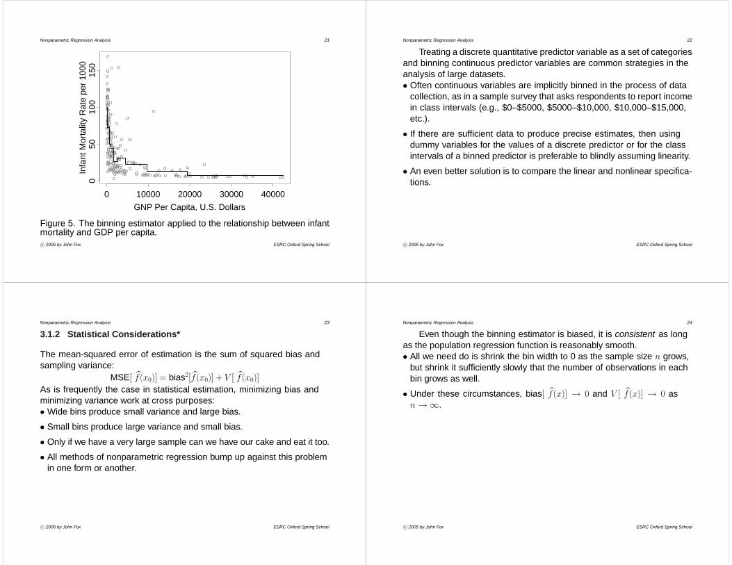
Figure 5 depicts the binning estimator applied to the U. N. infant-mortality data. The line in this graph employs 10 bins, each with roughly19 observations.



Infa

nt M

orta

lity

Rat

e pe

r 100

0

0 10000 20000 30000 40000

050

100

150

GNP Per Capita, U.S. Dollars

Figure 5. The binning estimator applied to the relationship between infantmortality and GDP per capita.c° 2005 by John Fox ESRC Oxford Spring School


Treating a discrete quantitative predictor variable as a set of categoriesand binning continuous predictor variables are common strategies in theanalysis of large datasets.• Often continuous variables are implicitly binned in the process of data

collection, as in a sample survey that asks respondents to report incomein class intervals (e.g., $0–$5000, $5000–$10,000, $10,000–$15,000,etc.).

• If there are sufficient data to produce precise estimates, then usingdummy variables for the values of a discrete predictor or for the classintervals of a binned predictor is preferable to blindly assuming linearity.

• An even better solution is to compare the linear and nonlinear specifica-tions.



3.1.2 Statistical Considerations*

The mean-squared error of estimation is the sum of squared bias andsampling variance:

MSE[ bf(x0)] = bias2[ bf(x0)] + V [ bf(x0)]As is frequently the case in statistical estimation, minimizing bias andminimizing variance work at cross purposes:• Wide bins produce small variance and large bias.

• Small bins produce large variance and small bias.

• Only if we have a very large sample can we have our cake and eat it too.

• All methods of nonparametric regression bump up against this problemin one form or another.



Even though the binning estimator is biased, it is consistent as longas the population regression function is reasonably smooth.• All we need do is shrink the bin width to 0 as the sample size n grows,

but shrink it sufficiently slowly that the number of observations in eachbin grows as well.

• Under these circumstances, bias[ bf(x)] → 0 and V [ bf(x)] → 0 asn→∞.



3.1.3 Local Averaging

The essential idea behind local averaging is that, as long as the regressionfunction is smooth, observations with x-values near a focal x0 areinformative about f(x0).• Local averaging is very much like binning, except that rather than

dissecting the data into non-overlapping bins, we move a bin (called awindow) continuously over the data, averaging the observations that fallin the window.

• We can calculate bf(x) at a number of focal values of x, usually equallyspread within the range of observed x-values, or at the (ordered)observations, x(1), x(2), ..., x(n).

• As in binning, we can employ a window of fixed width w centered on thefocal value x0, or can adjust the width of the window to include a constantnumber of observations, m. These are the m nearest neighbors of thefocal value.



• Problems occur near the extremes of the x’s. For example, all of thenearest neighbors of x(1) are greater than or equal to x(1), and thenearest neighbors of x(2) are almost surely the same as those of x(1),producing an artificial flattening of the regression curve at the extremeleft, called boundary bias. A similar flattening occurs at the extremeright, near x(n).

Figure 6 shows how local averaging works, using the relationship ofprestige to income in the Canadian occupational prestige data.

1. The window shown in panel (a) includes the m = 40 nearest neighborsof the focal value x(80).

2. The y-values associated with these observations are averaged,producing the fitted value by(80) in panel (b).

3. Fitted values are calculated for each focal x (in this case x(1), x(2), ..., x(102))and then connected, as in panel (c).



• In addition to the obvious flattening of the regression curve at the leftand right, local averages can be rough, because bf(x) tends to take smalljumps as observations enter and exit the window. The kernel estimator(described shortly) produces a smoother result.

• Local averages are also subject to distortion when outliers fall in thewindow, a problem addressed by robust estimation.



0 5000 10000 15000 20000 25000

2040

6080

(a)

Income

Pre

stig

e

x(80)

0 5000 10000 15000 20000 25000

2040

6080

(b)

Income

Pre

stig

e

x(80)

y(80)

0 5000 10000 15000 20000 25000

2040

6080

(c)

Income

Pre

stig

e

Figure 6. Nonparametric regression of prestige on income usinglocal averages.c° 2005 by John Fox ESRC Oxford Spring School


3.2 Kernel Estimation (Locally Weighted Averaging)

Kernel estimation is an extension of local averaging.• The essential idea is that in estimating f(x0) it is desirable to give greater

weight to observations that are close to the focal x0.

• Let zi = (xi − x0)/h denote the scaled, signed distance between thex-value for the ith observation and the focal x0. The scale factor h,called the bandwidth of the kernel estimator, plays a role similar to thewindow width of a local average.

• We need a kernel function K(z) that attaches greatest weight to obser-vations that are close to the focal x0, and then falls off symmetrically andsmoothly as |z| grows. Given these characteristics, the specific choiceof a kernel function is not critical.



• Having calculated weights wi = K[(xi − x0)/h], we proceed to computea fitted value at x0 by weighted local averaging of the y’s:bf(x0) = by|x0 = Pn

i=1wiyiPni=1wi

• Two popular choices of kernel functions, illustrated in Figure 7, are theGaussian or normal kernel and the tricube kernel:– The normal kernel is simply the standard normal density function,

KN(z) =1√2π

e−z2/2

Here, the bandwidth h is the standard deviation of a normal distributioncentered at x0.



K(z

)

-2 -1 0 1 2

0.0

0.2

0.4

0.6

0.8

1.0

Figure 7. Tricube (light solid line), normal (broken line, rescaled) and rec-tangular (heavy solid line) kernel functions.c° 2005 by John Fox ESRC Oxford Spring School


– The tricube kernel isKT (z) =

½(1− |z|3)3 for |z| < 1

0 for |z| ≥ 1For the tricube kernel, h is the half-width of a window centered at thefocal x0. Observations that fall outside of the window receive 0 weight.

– Using a rectangular kernel (also shown in Figure 7)

KR(z) =

½1 for |z| < 10 for |z| ≥ 1

gives equal weight to each observation in a window of half-width hcentered at x0, and therefore produces an unweighted local average.



I have implicitly assumed that the bandwidth h is fixed, but the kernelestimator is easily adapted to nearest-neighbour bandwidths.• The adaptation is simplest for kernel functions, like the tricube kernel,

that fall to 0: Simply adjust h(x) so that a fixed number of observationsm are included in the window.

• The fraction m/n is called the span of the kernel smoother.



Kernel estimation is illustrated in Figure 8 for the Canadian occupa-tional prestige data.• Panel (a) shows a neighborhood containing 40 observations centered on

the 80th ordered x-value.

• Panel (b) shows the tricube weight function defined on the window; thebandwidth h[x(80)] is selected so that the window that accommodates the40 nearest neighbors of the focal x(80). Thus, the span of the smootheris 40/102 ' .4.

• Panel (c) shows the locally weighted average, by(80) = by|x(80).• Panel (d) connects the fitted values to obtain the kernel estimate of the

regression of prestige on income. In comparison with the local-averageregression, the kernel estimate is smoother, but it still exhibits flatteningat the boundaries.



0 5000 10000 15000 20000 25000

2040

6080

(a)

Income

Pre

stig

e

x(80)

0 5000 10000 15000 20000 25000

0.0

0.2

0.4

0.6

0.8

1.0

(b)

Income

Tric

ube

Wei

ght

x(80)

0 5000 10000 15000 20000 25000

2040

6080

(c)

Income

Pre

stig

e

x(80)

y(80)

0 5000 10000 15000 20000 25000

2040

6080

(d)

Income

Pre

stig

e

Figure 8. The kernel estimator applied to the Canadian occupational pres-tige data.c° 2005 by John Fox ESRC Oxford Spring School


Varying the bandwidth of the kernel estimator controls the smoothnessof the estimated regression function: Larger bandwidths produce smootherresults. Choice of bandwidth will be discussed in more detail in connectionwith local polynomial regression.



3.3 Local Polynomial Regression

Local polynomial regression corrects some of the deficiencies of kernelestimation.• It provides a generally adequate method of nonparametric regression

that extends to multiple regression, additive regression, and generalizednonparametric regression.

• An implementation of local polynomial regression called lowess (orloess) is the most commonly available method of nonparametricregression.



Perhaps you are familiar with polynomial regression, where a p-degreepolynomial in a predictor x,

y = α + β1x + β2x2 + · · · + βpx

p + ε

is fit to data, usually by the method of least squares:• p = 1 corresponds to a linear fit, p = 2 to a quadratic fit, and so on.

• Fitting a constant (i.e., the mean) corresponds to p = 0.



Local polynomial regression extends kernel estimation to a polynomialfit at the focal point x0, using local kernel weights, wi = K[(xi − x0)/h].The resulting weighted least-squares (WLS) regression fits the equation

yi = a+ b1(xi − x0) + b2(xi − x0)2 + · · · + bp(xi − x0)

p + eito minimize the weighted residual sum of squares,

Pni=1wie

2i .

• Once the WLS solution is obtained, the fitted value at the focal x0 is justby|x0 = a.

• As in kernel estimation, this procedure is repeated for representativefocal values of x, or at the observations xi.

• The bandwidth h can either be fixed or it can vary as a function of thefocal x.

• When the bandwidth defines a window of nearest neighbors, as isthe case for tricube weights, it is convenient to specify the degree ofsmoothing by the proportion of observations included in the window.This fraction s is called the span of the local-regression smoother.



• The number of observations included in each window is then m =[sn], where the square brackets denote rounding to the nearest wholenumber.

Selecting p = 1 produces a local linear fit, the most common case.• The ‘tilt’ of the local linear fit promises reduced bias in comparison with

the kernel estimator, which corresponds to p = 0. This advantage ismost apparent at the boundaries, where the kernel estimator tends toflatten.

• The values p = 2 or p = 3, local quadratic or cubic fits, produce moreflexible regressions. Greater flexibility has the potential to reduce biasfurther, but flexibility also entails the cost of greater variation.

• There is a theoretical advantage to odd-order local polynomials, so p = 1is generally preferred to p = 0, and p = 3 to p = 2.



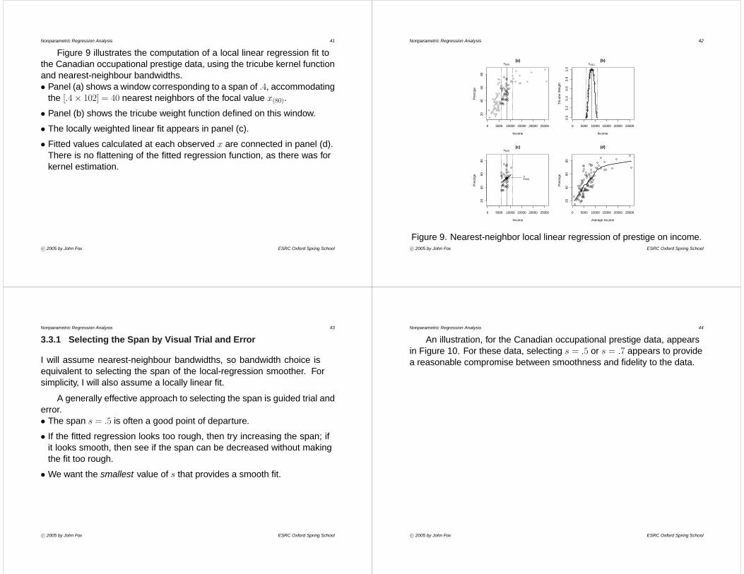
Figure 9 illustrates the computation of a local linear regression fit tothe Canadian occupational prestige data, using the tricube kernel functionand nearest-neighbour bandwidths.• Panel (a) shows a window corresponding to a span of .4, accommodating

the [.4× 102] = 40 nearest neighbors of the focal value x(80).

• Panel (b) shows the tricube weight function defined on this window.

• The locally weighted linear fit appears in panel (c).

• Fitted values calculated at each observed x are connected in panel (d).There is no flattening of the fitted regression function, as there was forkernel estimation.



0 5000 10000 15000 20000 25000

2040

6080

(a)

Income

Pre

stig

e

x(80)

0 5000 10000 15000 20000 25000

0.0

0.2

0.4

0.6

0.8

1.0

(b)

Income

Tric

ube

Wei

ght

x(80)

0 5000 10000 15000 20000 25000

2040

6080

(c)

Income

Pre

stig

e

x(80)

y(80)

0 5000 10000 15000 20000 25000

2040

6080

(d)

Average Income

Pre

stig

e

Figure 9. Nearest-neighbor local linear regression of prestige on income.c° 2005 by John Fox ESRC Oxford Spring School


3.3.1 Selecting the Span by Visual Trial and Error

I will assume nearest-neighbour bandwidths, so bandwidth choice isequivalent to selecting the span of the local-regression smoother. Forsimplicity, I will also assume a locally linear fit.

A generally effective approach to selecting the span is guided trial anderror.• The span s = .5 is often a good point of departure.

• If the fitted regression looks too rough, then try increasing the span; ifit looks smooth, then see if the span can be decreased without makingthe fit too rough.

• We want the smallest value of s that provides a smooth fit.



An illustration, for the Canadian occupational prestige data, appearsin Figure 10. For these data, selecting s = .5 or s = .7 appears to providea reasonable compromise between smoothness and fidelity to the data.



0 5000 10000 15000 20000 25000

2040

6080

s= 0.1

Income

Pres

tige

0 5000 10000 15000 20000 25000

2040

6080

s= 0.3

Income

Pres

tige

0 5000 10000 15000 20000 25000

2040

6080

s= 0.5

Income

Pres

tige

0 5000 10000 15000 20000 25000

2040

6080

s= 0.7

Income

Pres

tige

0 5000 10000 15000 20000 25000

2040

6080

s= 0.9

Income

Pres

tige

Figure 10. Nearest-neighbor local linear regression of prestige on income,for several values of the span s.c° 2005 by John Fox ESRC Oxford Spring School


3.3.2 Selecting the Span by Cross-Validation*

A conceptually appealing, but complex, approach to bandwidth selectionis to estimate the optimal h (say h∗). We either need to estimate h∗(x0)for each value x0 of x at which by|x is to be evaluated, or to estimate anoptimal average value to be used with the fixed-bandwidth estimator. Asimilar approach is applicable to the nearest-neighbour local-regressionestimator.• The so-called plug-in estimate of h∗ proceeds by estimating its compo-

nents, which are the error variance σ2, the curvature of the regressionfunction at the focal x0, and the density of x-values at x0. To do thisrequires a preliminary estimate of the regression function.



• A simpler approach is to estimate the optimal bandwidth or span bycross-validation In cross-validation, we evaluate the regression functionat the observations xi.– The key idea in cross-validation is to omit the ith observation from the

local regression at the focal value xi. We denote the resulting estimateof E(y|xi) as by−i|xi. Omitting the ith observation makes the fitted valueby−i|xi independent of the observed value yi.

– The cross-validation function is

CV(s) =Pn

i=1 [by−i(s)− yi]2

nwhere by−i(s) is by−i|xi for span s. The object is to find the value of sthat minimizes CV.

– In practice, we need to compute CV(s) for a range of values of s.– Other than repeating the local-regression fit for different values ofs, cross-validation does not increase the burden of computation,because we typically evaluate the local regression at each xi anyway.



– Although cross-validation is often a useful method for selectingthe span, CV(s) is only an estimate, and is therefore subject tosampling variation. Particularly in small samples, this variability canbe substantial. Moreover, the approximations to the expectation andvariance of the local-regression estimator are asymptotic, and in smallsamples CV(s) often provides values of s that are too small.

– There are sophisticated generalizations of cross-validation that arebetter behaved.

Figure 11 shows CV(s) for the regression of occupational prestige onincome. In this case, the cross-validation function provides little specifichelp in selecting the span, suggesting simply that s should be relativelylarge. Compare this with the value s ' .6 that we arrived at by visual trialand error.



CV(

s)

0.0 0.2 0.4 0.6 0.8 1.0

100

150

200

250

Figure 11. Cross-validation function for the local linear regression of pres-tige on income.c° 2005 by John Fox ESRC Oxford Spring School


3.4 Making Local Regression Resistant to Outliers*

As in linear least-squares regression, outliers — and the heavy-tailederror distributions that generate them — can wreak havoc with thelocal-regression least-squares estimator.• One solution is to down-weight outlying observations. In linear regres-

sion, this strategy leads to M -estimation, a kind of robust regression.

• The same strategy is applicable to local polynomial regression.

Suppose that we fit a local regression to the data, obtaining estimatesbyi and residuals ei = yi − byi.• Large residuals represent observations that are relatively remote from

the fitted regression.



• Now define weights Wi = W (ei), where the symmetric function W (·)assigns maximum weight to residuals of 0, and decreasing weight as theabsolute residuals grow.– One popular choice of weight function is the bisquare or biweight :

Wi =WB(ei) =

⎧⎨⎩∙1−

³ eicS

´2¸2for |ei| < cS

0 for |ei| ≥ cSwhere S is a measure of spread of the residuals, such as S =median|ei|; and c is a tuning constant.

– Smaller values of c produce greater resistance to outliers but lowerefficiency when the errors are normally distributed.

– Selecting c = 7 and using the median absolute deviation producesabout 95-percent efficiency compared with least-squares when theerrors are normal; the slightly smaller value c = 6 is usually used.



– Another common choice is the Huber weight function:

Wi =WH(ei) =

½1 for |ei| ≤ cS

cS/|ei| for |ei| > cSUnlike the biweight, the Huber weight function never quite reaches 0.

– The tuning constant c = 2 produces roughly 95-percent efficiency fornormally distributed errors.

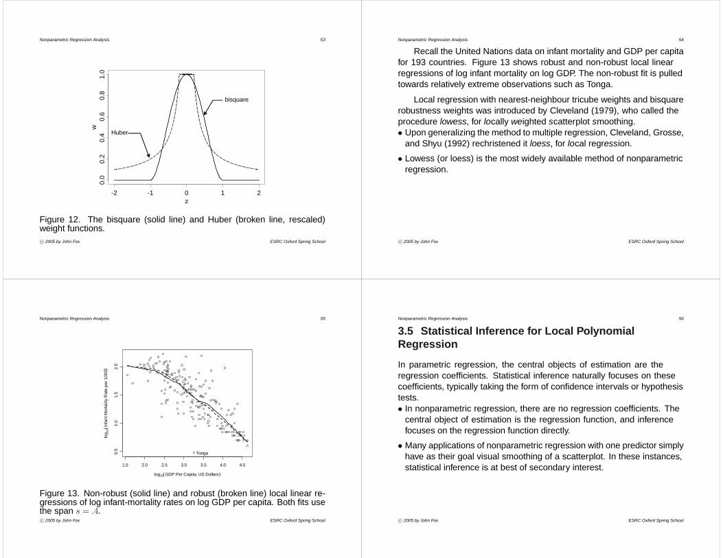
The bisquare and Huber weight functions are graphed in Figure 12.

• We refit the local regression at the focal values xi by WLS, minimizingthe weighted residual sum of squares

Pni=1wiWie

2i , where the Wi

are the ‘robustness’ weights, just defined, and the wi are the kernel‘neighborhood’ weights.

• Because an outlier will influence the initial local fits, residuals androbustness weights, it is necessary to iterate this procedure until thefitted values byi stop changing. Two to four robustness iterations almostalways suffice.



w

-2 -1 0 1 2

0.0

0.2

0.4

0.6

0.8

1.0

bisquare

Huber

Figure 12. The bisquare (solid line) and Huber (broken line, rescaled)weight functions.c° 2005 by John Fox ESRC Oxford Spring School


Recall the United Nations data on infant mortality and GDP per capitafor 193 countries. Figure 13 shows robust and non-robust local linearregressions of log infant mortality on log GDP. The non-robust fit is pulledtowards relatively extreme observations such as Tonga.

Local regression with nearest-neighbour tricube weights and bisquarerobustness weights was introduced by Cleveland (1979), who called theprocedure lowess, for locally weighted scatterplot smoothing.• Upon generalizing the method to multiple regression, Cleveland, Grosse,

and Shyu (1992) rechristened it loess, for local regression.

• Lowess (or loess) is the most widely available method of nonparametricregression.



1.5 2.0 2.5 3.0 3.5 4.0 4.5

0.5

1.0

1.5

2.0

log10(GDP Per Capita, US Dollars)

log 1

0(In

fant

Mor

talit

y R

ate

per 1

000 )

Tonga

Figure 13. Non-robust (solid line) and robust (broken line) local linear re-gressions of log infant-mortality rates on log GDP per capita. Both fits usethe span s = .4.c° 2005 by John Fox ESRC Oxford Spring School


3.5 Statistical Inference for Local PolynomialRegression

In parametric regression, the central objects of estimation are theregression coefficients. Statistical inference naturally focuses on thesecoefficients, typically taking the form of confidence intervals or hypothesistests.• In nonparametric regression, there are no regression coefficients. The

central object of estimation is the regression function, and inferencefocuses on the regression function directly.

• Many applications of nonparametric regression with one predictor simplyhave as their goal visual smoothing of a scatterplot. In these instances,statistical inference is at best of secondary interest.



3.5.1 Confidence Envelopes*

Consider the local polynomial estimate by|x of the regression functionf(x). For notational convenience, I assume that the regression function isevaluated at the observed predictor values, x1, x2, ..., xn.• The fitted value byi = by|xi results from a locally weighted least-squares

regression of y on the x values. This fitted value is therefore a weightedsum of the observations: byi = nX

j=1

sijyj

where the weights sij are functions of the x-values.



• Because (by assumption) the yi’s are independently distributed, withcommon conditional variance V (y|x = xi) = V (yi) = σ2, the samplingvariance of the fitted value byi is

V (byi) = σ2nX

j=1

s2ij

• To apply this result, we require an estimate of σ2. In linear least-squaressimple regression, we estimate the error variance as

S2 =

Pe2i

n− 2where ei = yi − byi is the residual for observation i, and n − 2 is thedegrees of freedom associated with the residual sum of squares.

• We can calculate residuals in nonparametric regression in the samemanner — that is, ei = yi − byi.



• To complete the analogy, we require the equivalent number of parame-ters or equivalent degrees of freedom for the model, dfmod, from whichwe can obtain the residual degrees of freedom, dfres = n− dfmod.

• Then, the estimated error variance is

S2 =

Pe2i

dfresand the estimated variance of the fitted value byi at x = xi isbV (byi) = S2

nXj=1

s2ij

• Assuming normally distributed errors, or a sufficiently large sample,a 95-percent confidence interval for E(y|xi) = f(xi) is approximatelybyi ± 2qbV (byi)



• Putting the confidence intervals together for x = x1, x2, ..., xn producesa pointwise 95-percent confidence band or confidence envelope for theregression function.

An example, employing the local linear regression of prestige onincome in the Canadian occupational prestige data (with span s = .6),appears in Figure 14. Here, dfmod = 5.0, and S2 = 12, 004.72/(102 −5.0) = 123.76. The nonparametric-regression smooth therefore uses theequivalent of 5 parameters.



Pre

stig

e

0 5000 10000 15000 20000 25000

2040

6080

Figure 14. Local linear regression of occupational prestige on income,showing an approximate point-wise 95-percent confidence envelope.c° 2005 by John Fox ESRC Oxford Spring School


The following three points should be noted:

1. Although the locally linear fit uses the equivalent of 5 parameters,it does not produce the same regression curve as fitting a globalfourth-degree polynomial to the data.

2. In this instance, the equivalent number of parameters rounds to aninteger, but this is an accident of the example.

3. Because by|x is a biased estimate of E(y|x), it is more accurate todescribe the envelope around the sample regression as a “variabilityband” rather than as a confidence band.



3.5.2 Hypothesis Tests

In linear least-squares regression, F -tests of hypotheses are formulatedby comparing alternative nested models.• To say that two models are nested means that one, the more specific

model, is a special case of the other, more general model.

• For example, in least-squares linear simple regression, the F -statistic

F =TSS− RSSRSS/(n− 2)

with 1 and n − 2 degrees of freedom tests the hypothesis of no linearrelationship between y and x.– The total sum of squares, TSS =

P(yi − y)2, is the variation in y

associated with the null model of no relationship, yi = α + εi;– the residual sum of squares, RSS =

P(yi − byi)2, represents the

variation in y conditional on the linear relationship between y and x,based the model yi = α + βxi + εi.



– Because the null model is a special case of the linear model, withβ = 0, the two models are (heuristically) nested.

• An analogous, but more general, F -test of no relationship for thenonparametric-regression model is

F =(TSS− RSS)/(dfmod − 1)

RSS/dfreswith dfmod − 1 and dfres = n− dfmod degrees of freedom.– Here RSS is the residual sum of squares for the nonparametric

regression model.– Applied to the local linear regression of prestige on income, using

the loess function in R with a span of 0.6, where n = 102, TSS= 29, 895.43, RSS = 12, 041.37, and dfmod = 4.3, we have

F =(29, 895.43− 12, 041.37)/(4.3− 1)

12, 041.37/(102− 4.3) = 43.90

with 4.3 − 1 = 3.3 and 102 − 4.3 = 97.7 degrees of freedom. Theresulting p-value is much smaller than .0001.



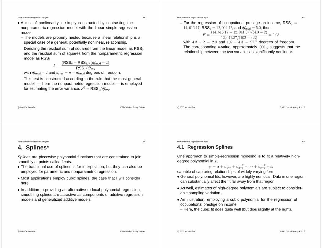
• A test of nonlinearity is simply constructed by contrasting thenonparametric-regression model with the linear simple-regressionmodel.– The models are properly nested because a linear relationship is a

special case of a general, potentially nonlinear, relationship.– Denoting the residual sum of squares from the linear model as RSS0

and the residual sum of squares from the nonparametric regressionmodel as RSS1,

F =(RSS0 − RSS1)/(dfmod − 2)

RSS1/dfreswith dfmod − 2 and dfres = n− dfmod degrees of freedom.

– This test is constructed according to the rule that the most generalmodel — here the nonparametric-regression model — is employedfor estimating the error variance, S2 = RSS1/dfres.



– For the regression of occupational prestige on income, RSS0 =14, 616.17, RSS1 = 12, 004.72, and dfmod = 5.0; thus

F =(14, 616.17− 12, 041.37)/(4.3− 2)

12, 041.37/(102− 4.3) = 9.08

with 4.3 − 2 = 2.3 and 102 − 4.3 = 97.7 degrees of freedom.The corresponding p-value, approximately .0001, suggests that therelationship between the two variables is significantly nonlinear.



4. Splines*Splines are piecewise polynomial functions that are constrained to joinsmoothly at points called knots.• The traditional use of splines is for interpolation, but they can also be

employed for parametric and nonparametric regression.

• Most applications employ cubic splines, the case that I will considerhere.

• In addition to providing an alternative to local polynomial regression,smoothing splines are attractive as components of additive regressionmodels and generalized additive models.



4.1 Regression Splines

One approach to simple-regression modeling is to fit a relatively high-degree polynomial in x,

yi = α + β1xi + β2x2i + · · · + βpx

pi + εi

capable of capturing relationships of widely varying form.• General polynomial fits, however, are highly nonlocal: Data in one region

can substantially affect the fit far away from that region.

• As well, estimates of high-degree polynomials are subject to consider-able sampling variation.

• An illustration, employing a cubic polynomial for the regression ofoccupational prestige on income:– Here, the cubic fit does quite well (but dips slightly at the right).



0 5000 10000 15000 20000 2500020

4060

80

(a) Cubic

Income

Pre

stig

e

0 5000 10000 15000 20000 25000

2040

6080

(b) Piecewise Cubics

Income

Pre

stig

e

0 5000 10000 15000 20000 25000

2040

6080

(c) Natural Cubic Spline

Income

Pre

stig

e

Figure 15. Polynomial fits to the Canadian occupational prestige data: (a)a global cubic fit; (b) independent cubic fits in two bins, divided at Income= 10, 000; (c) a natural cubic spline, with one knot at Income = 10, 000.c° 2005 by John Fox ESRC Oxford Spring School


As an alternative, we can partition the data into bins, fitting a differentpolynomial regression in each bin.• A defect of this piecewise procedure is that the curves fit to the different

bins will almost surely be discontinuous, as illustrated in Figure 15 (b).

• Cubic regression splines fit a third-degree polynomial in each bin underthe added constraints that the curves join at the bin boundaries (theknots), and that the first and second derivatives (i.e., the slope andcurvature of the regression function) are continuous at the knots.

• Natural cubic regression splines add knots at the boundaries of thedata, and impose the additional constraint that the fit is linear beyondthe terminal knots.– This requirement tends to avoid wild behavior near the extremes of the

data.– If there are k ‘interior’ knots and two knots at the boundaries, the

natural spline uses k + 2 independent parameters.



– With the values of the knots fixed, a regression spline is just a linearmodel, and as such provides a fully parametric fit to the data.

– Figure 15 (c) shows the result of fitting a natural cubic regressionspline with one knot at Income = 10, 000, the location of which wasdetermined by examining the scatterplot, and the model thereforeuses only 3 parameters.



4.2 Smoothing Splines

In contrast to regression splines, smoothing splines arise as the solutionto the following nonparametric-regression problem: Find the functionbf(x) with two continuous derivatives that minimizes the penalized sum ofsquares,

SS∗(h) =nXi=1

[yi − f(xi)]2 + h

Z xmax

xmin

[f 00(x)]2 dx

where h is a smoothing constant, analogous to the bandwidth of a kernelor local-polynomial estimator.• The first term in the equation is the residual sum of squares.

• The second term is a roughness penalty, which is large when theintegrated second derivative of the regression function f 00(x) is large —that is, when f(x) is rough.



• If h = 0 then bf(x) simply interpolates the data.

• If h is very large, then bf will be selected so that bf 00(x) is everywhere 0,which implies a globally linear least-squares fit to the data.



It turns out that the function bf(x) that minimizes SS∗(h) is a naturalcubic spline with knots at the distinct observed values of x.• Although this result seems to imply that n parameters are required,

the roughness penalty imposes additional constraints on the solution,typically reducing the equivalent number of parameters for the smoothingspline greatly.– It is common to select the smoothing constant h indirectly by setting

the equivalent number of parameters for the smoother.– An illustration appears in Figure 16, comparing a smoothing spline with

a local-linear fit employing the same equivalent number of parameters(degrees of freedom).

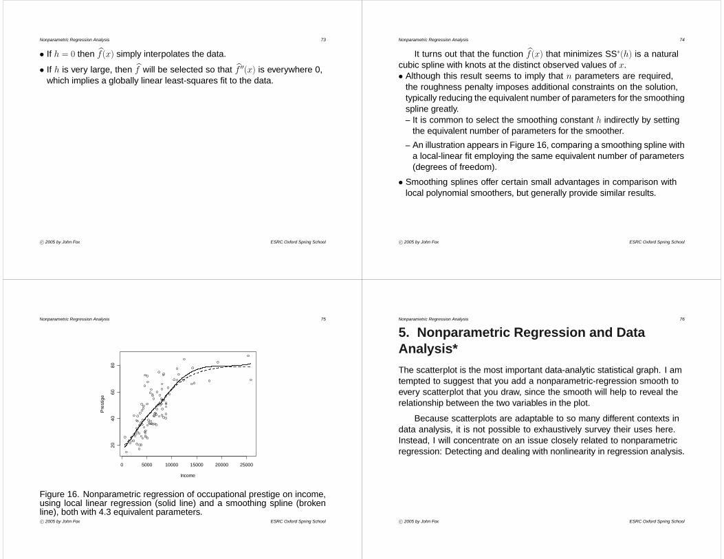
• Smoothing splines offer certain small advantages in comparison withlocal polynomial smoothers, but generally provide similar results.



0 5000 10000 15000 20000 25000

2040

6080

Income

Pre

stig

e

Figure 16. Nonparametric regression of occupational prestige on income,using local linear regression (solid line) and a smoothing spline (brokenline), both with 4.3 equivalent parameters.c° 2005 by John Fox ESRC Oxford Spring School


5. Nonparametric Regression and DataAnalysis*The scatterplot is the most important data-analytic statistical graph. I amtempted to suggest that you add a nonparametric-regression smooth toevery scatterplot that you draw, since the smooth will help to reveal therelationship between the two variables in the plot.

Because scatterplots are adaptable to so many different contexts indata analysis, it is not possible to exhaustively survey their uses here.Instead, I will concentrate on an issue closely related to nonparametricregression: Detecting and dealing with nonlinearity in regression analysis.



• One response to the possibility of nonlinearity is to employ nonparamet-ric multiple regression.

• An alternative is to fit a preliminary linear regression; to employappropriate diagnostic plots to detect departures from linearity; andto follow up by specifying a new parametric model that capturesnonlinearity detected in the diagnostics, for example by transforming apredictor.



5.1 The ‘Bulging Rule’

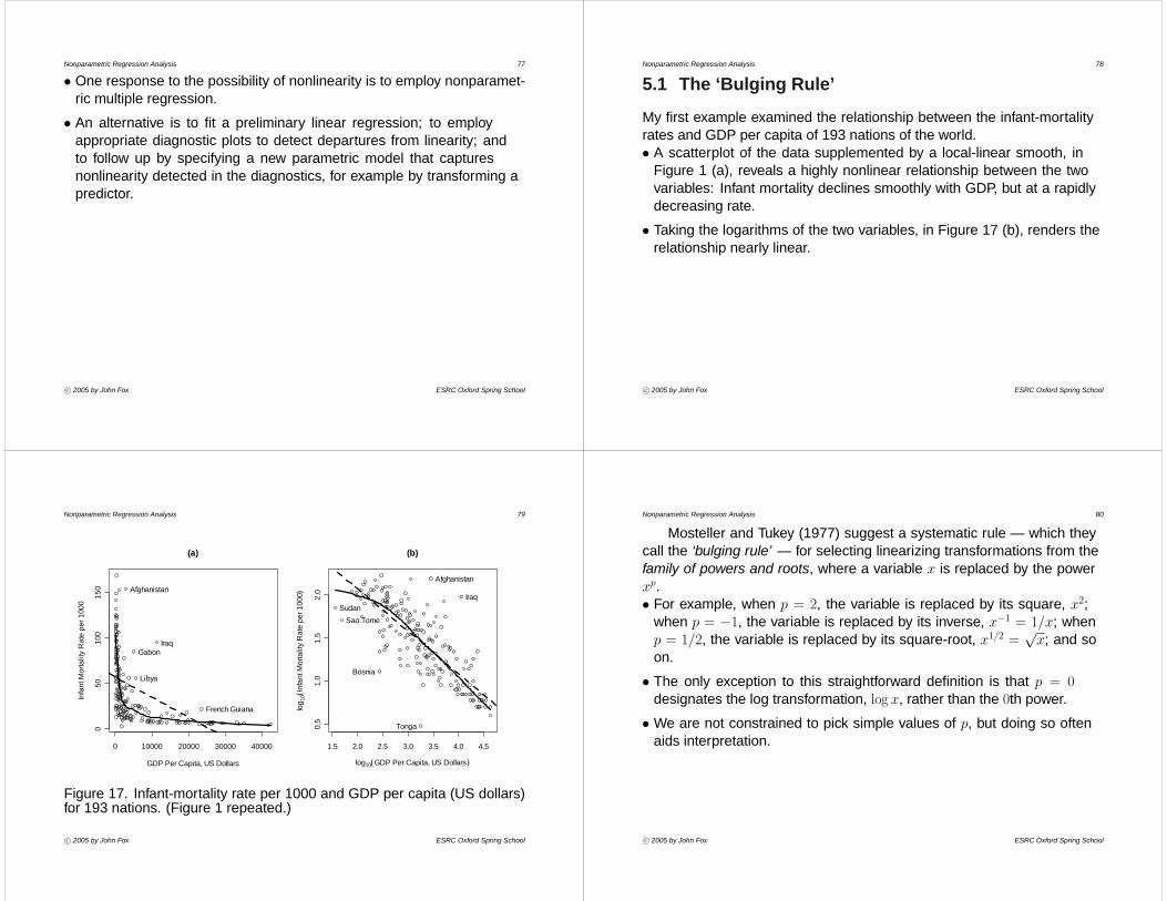
My first example examined the relationship between the infant-mortalityrates and GDP per capita of 193 nations of the world.• A scatterplot of the data supplemented by a local-linear smooth, in

Figure 1 (a), reveals a highly nonlinear relationship between the twovariables: Infant mortality declines smoothly with GDP, but at a rapidlydecreasing rate.

• Taking the logarithms of the two variables, in Figure 17 (b), renders therelationship nearly linear.



0 10000 20000 30000 40000

050

100

150

(a)

GDP Per Capita, US Dollars

Infa

nt M

orta

lity

Rat

e pe

r 100

0

Afghanistan

French.Guiana

GabonIraq

Libya

1.5 2.0 2.5 3.0 3.5 4.0 4.5

0.5

1.0

1.5

2.0

(b)

log10(GDP Per Capita, US Dollars)

log 1

0(In

fant

Mor

talit

y R

ate

per 1

000 )

Afghanistan

Bosnia

Iraq

Sao.TomeSudan

Tonga

Figure 17. Infant-mortality rate per 1000 and GDP per capita (US dollars)for 193 nations. (Figure 1 repeated.)



Mosteller and Tukey (1977) suggest a systematic rule — which theycall the ‘bulging rule’ — for selecting linearizing transformations from thefamily of powers and roots, where a variable x is replaced by the powerxp.• For example, when p = 2, the variable is replaced by its square, x2;

when p = −1, the variable is replaced by its inverse, x−1 = 1/x; whenp = 1/2, the variable is replaced by its square-root, x1/2 =

√x; and so

on.

• The only exception to this straightforward definition is that p = 0designates the log transformation, log x, rather than the 0th power.

• We are not constrained to pick simple values of p, but doing so oftenaids interpretation.



• Transformations in the family of powers and roots are only applicablewhen all of the values of x are positive:– Some of the transformations, such as square-root and log, are

undefined for negative values of x.– Other transformations, such as x2, would distort the order of x if somex-values are negative and some are positive.

• A simple solution is to use a ‘start’ — to add a constant quantity c to allvalues of x prior to applying the power transformation: x→ (x + c)p.

• Notice that negative powers — such as the inverse transformation, x−1— reverse the order of the x-values; if we want to preserve the originalorder, then we can take x→ −xp when p is negative.

• Alternatively, we can use the similarly shaped Box-Cox family oftransformations:

x→ x(p) =

½(xp − 1)/p for p 6= 0loge x for p = 0



Power transformation of x or y can help linearize a nonlinearrelationship that is both simple and monotone. What is meant by theseterms is illustrated in Figure 18:• A relationship is simple when it is smoothly curved and when the

curvature does not change direction.

• A relationship is monotone when y strictly increases or decreases withx.– Thus, the relationship in Figure 18 (a) is simple and monotone;– the relationship in Figure 18 (b) is monotone but not simple, since the

direction of curvature changes from opening up to opening down;– the relationship in Figure 18 (c) is simple but nonmonotone, since y

first decreases and then increases with x.



x

y

x

y

x

y

(a)

(b) (c)

Figure 18. The relationship in (a) is simple and monotone; that in (b) ismontone but not simple; and that in (c) is simple but nonmonotone.c° 2005 by John Fox ESRC Oxford Spring School


Although nonlinear relationships that are not simple or that arenonmonotone cannot be linearized by a power transformation, other formsof parametric regression may be applicable. For example, the relationshipin Figure 18 (c) could be modeled as a quadratic equation:

y = α + β1x + β2x2 + ε

• Polynomial regression models, such as quadratic equations, can be fitby linear least-squares regression.

• Nonlinear least squares can be used to fit an even broader class ofparametric models.



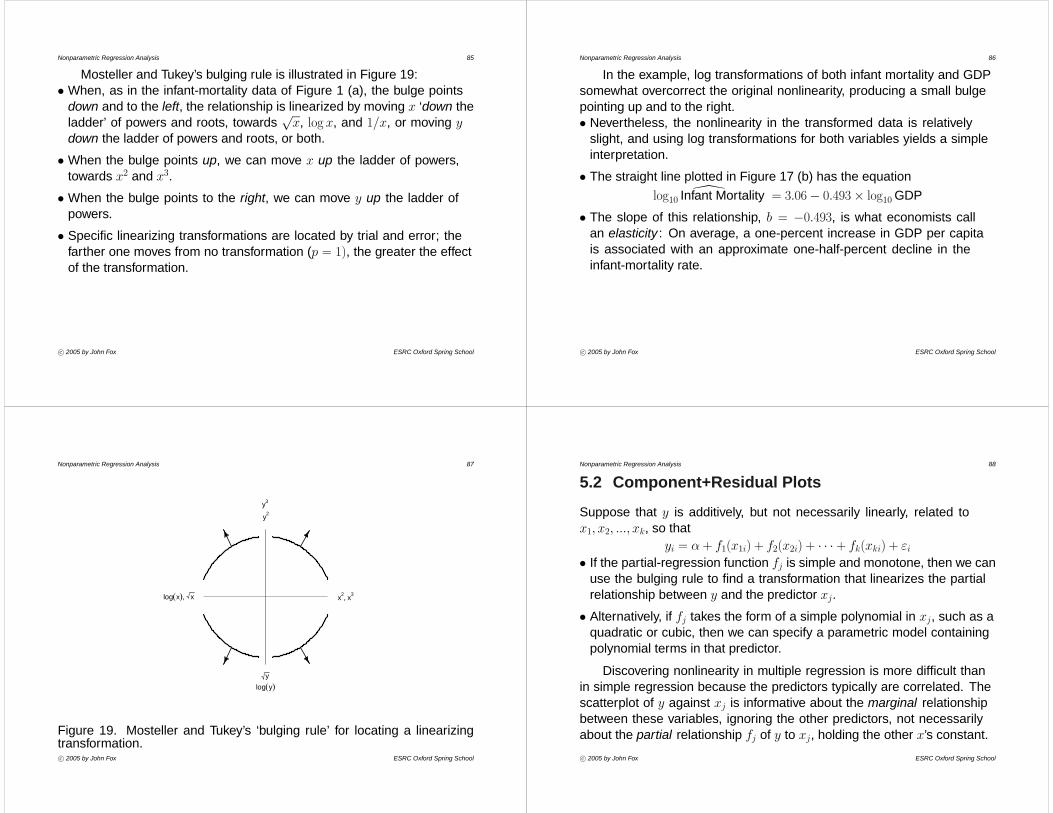
Mosteller and Tukey’s bulging rule is illustrated in Figure 19:• When, as in the infant-mortality data of Figure 1 (a), the bulge points

down and to the left, the relationship is linearized by moving x ‘down theladder’ of powers and roots, towards

√x, log x, and 1/x, or moving y

down the ladder of powers and roots, or both.

• When the bulge points up, we can move x up the ladder of powers,towards x2 and x3.

• When the bulge points to the right, we can move y up the ladder ofpowers.

• Specific linearizing transformations are located by trial and error; thefarther one moves from no transformation (p = 1), the greater the effectof the transformation.



In the example, log transformations of both infant mortality and GDPsomewhat overcorrect the original nonlinearity, producing a small bulgepointing up and to the right.• Nevertheless, the nonlinearity in the transformed data is relatively

slight, and using log transformations for both variables yields a simpleinterpretation.

• The straight line plotted in Figure 17 (b) has the equation\log10 Infant Mortality = 3.06− 0.493× log10GDP

• The slope of this relationship, b = −0.493, is what economists callan elasticity : On average, a one-percent increase in GDP per capitais associated with an approximate one-half-percent decline in theinfant-mortality rate.



x2, x3log(x), x

y2

y3

ylog(y)

Figure 19. Mosteller and Tukey’s ‘bulging rule’ for locating a linearizingtransformation.c° 2005 by John Fox ESRC Oxford Spring School


5.2 Component+Residual Plots

Suppose that y is additively, but not necessarily linearly, related tox1, x2, ..., xk, so that

yi = α + f1(x1i) + f2(x2i) + · · · + fk(xki) + εi• If the partial-regression function fj is simple and monotone, then we can

use the bulging rule to find a transformation that linearizes the partialrelationship between y and the predictor xj.

• Alternatively, if fj takes the form of a simple polynomial in xj, such as aquadratic or cubic, then we can specify a parametric model containingpolynomial terms in that predictor.

Discovering nonlinearity in multiple regression is more difficult thanin simple regression because the predictors typically are correlated. Thescatterplot of y against xj is informative about the marginal relationshipbetween these variables, ignoring the other predictors, not necessarilyabout the partial relationship fj of y to xj, holding the other x’s constant.c° 2005 by John Fox ESRC Oxford Spring School


Under relatively broad circumstances component+residual plots (alsocalled partial-residual plots) can help to detect nonlinearity in multipleregression.• We fit a preliminary linear least-squares regression,

yi = a+ b1x1i + b2x2i + · · · + bkxki + ei

• The partial residuals for xj add the least-squares residuals to the linearcomponent of the relationship between y and xj:

ei[j] = ei + bjxji

• An unmodeled nonlinear component of the relationship between yand xj should appear in the least-squares residuals, so plotting andsmoothing e[j] against xj will reveal the partial relationship between y

and xj. We think of the smoothed partial-residual plot as an estimate bfjof the partial-regression function.

• This procedure is repeated for each predictor, j = 1, 2, ..., k.



Illustrative component+residual plots appear in Figure 20, for theregression of prestige on income and education.• The solid line on each plot gives a local-linear fit for span s = .6.

• the broken line gives the linear least-squares fit, and represents theleast-squares multiple-regression plane viewed edge-on in the directionof the corresponding predictor.



0 5000 10000 15000 20000 25000

-20

-10

010

20

income

Com

pone

nt+R

esid

ual(p

rest

ige)

6 8 10 12 14 16

-20

-10

010

2030

education

Com

pone

nt+R

esid

ual(p

rest

ige)

Figure 20. Component+residual plots for the regression of occupationalprestige on income and education.



• The left panel shows that the partial relationship between prestige andincome controlling for education is substantially nonlinear. Although thenonparametric regression curve fit to the plot is not altogether smooth,the bulge points up and to the left, suggesting transforming incomedown the ladder of powers and roots. Visual trial and error indicates thatthe log transformation of income serves to straighten the relationshipbetween prestige and income.

• The right panel suggests that the partial relationship between prestigeand education is nonlinear and monotone, but not simple. Consequently,a power transformation of education is not promising. We couldtry specifying a cubic regression for education (including education,education2, and education3 in the regression model), but the departurefrom linearity is slight, and a viable alternative here is simply to treat theeducation effect as linear.



• Regressing occupational prestige on education and the log (base 2) ofincome produces the following result:

\Prestige = −95.2 + 7.93× log2 Income+ 4.00× Education– Holding education constant, doubling income (i.e., increasinglog2Income by 1) is associated on average with an increment inprestige of about 8 points;

– holding income constant, increasing education by 1 year is associatedon average with an increment in prestige of 4 points.



6. Nonparametric Multiple RegressionI will describe two generalizations of nonparametric regression to two ormore predictors:

1. The local polynomial multiple-regression smoother, which fits thegeneral model

yi = f(x1i, x2i, ..., xki) + εi

2. The additive nonparametric regression modelyi = α + f1(x1i) + f2(x2i) + · · · + fk(xki) + εi



6.1 Local Polynomial Multiple Regression

As a formal matter, it is simple to extend the local-polynomial estimator toseveral predictors:• To obtain a fitted value by|x0 at the focal point x0 = (x1,0, x2,0, ..., xk0)0 in

the predictor space, we perform a weighted-least-squares polynomialregression of y on the x’s, emphasizing observations close to the focalpoint.– A local linear fit takes the form:

yi = a + b1(x1i − x1,0) + b2(x2i − x2,0)

+ · · · + bk(xki − xk0) + ei



– For k = 2 predictors, a local quadratic fit takes the formyi = a + b1(x1i − x1,0) + b2(x2i − x2,0)

+b11(x1i − x1,0)2 + b22(x2i − x2,0)

2

+b12(x1i − x1,0)(x2i − x2,0) + eiWhen there are several predictors, the number of terms in the localquadratic regression grows large, and consequently I will not considercubic or higher-order polynomials.

– In either the linear or quadratic case, we minimize the weighted sumof squares

Pni=1wie

2i for suitably defined weights wi. The fitted value

at the focal point in the predictor space is then by|x0 = a.



6.1.1 Finding Kernel Weights in Multiple Regression*

• There are two straightforward ways to extend kernel weighting to localpolynomial multiple regression:(a) Calculate marginal weights separately for each predictor,

wij = K[(xji − xj0)/hj]

Thenwi = wi1wi2 · · ·wik

(b) Measure the distance D(xi,x0) in the predictor space between thepredictor values xi for observation i and the focal x0. Then

wi = K

∙D(xi,x0)

h

¸There is, however, more than one way to define distances betweenpoints in the predictor space:



∗ Simple Euclidean distance:

DE(xi,x0) =

vuut kXj=1

(xji − xj0)2

Euclidean distances only make sense when the x’s are measuredin the same units (e.g., for spatially distributed data, where the twopredictors x1 and x2 represents coordinates on a map).∗ Scaled Euclidean distance: Scaled distances adjust each x by a

measure of dispersion to make values of the predictors comparable.For example,

zji =xji − xj

sjwhere xj and sj are the mean and standard deviation of xj. Then

DS(xi,x0) =

vuut kXj=1

(zji − zj0)2

This is the most common approach to defining distances.c° 2005 by John Fox ESRC Oxford Spring School


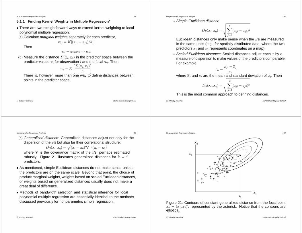
(c) Generalized distance: Generalized distances adjust not only for thedispersion of the x’s but also for their correlational structure:

DG(xi,x0) =p(xi − x0)0V−1(xi − x0)

where V is the covariance matrix of the x’s, perhaps estimatedrobustly. Figure 21 illustrates generalized distances for k = 2predictors.

• As mentioned, simple Euclidean distances do not make sense unlessthe predictors are on the same scale. Beyond that point, the choice ofproduct marginal weights, weights based on scaled Euclidean distances,or weights based on generalized distances usually does not make agreat deal of difference.

• Methods of bandwidth selection and statistical inference for localpolynomial multiple regression are essentially identical to the methodsdiscussed previously for nonparametric simple regression.



X1

X2

ooo

o

o

ooo

o

o

o

oo

o

oo

o

o

oo

oo

oo

o oo

o

o

o

oo

oo

o

o

o

o

o

o o

o

o

o

o

o

oo

o

o

o

o

o

o

o

o

o o

oo

o

o

ooo

o

o

o

o

o

oo

oo

o

o

o o

o

o

o

o

o

o

oo

oo

oo

o

o o ooo

o

oo

*

x1

x2

Figure 21. Contours of constant generalized distance from the focal pointx0 = (x1, x2)

0, represented by the asterisk. Notice that the contours areelliptical.



6.1.2 Obstacles to Nonparametric Multiple Regression

Although it is therefore simple to extend local polynomial estimation tomultiple regression, there are two flies in the ointment:

1. The ‘curse of dimensionality’: As the number of predictors increases,the number of observations in the local neighborhood of a focal pointtends to decline rapidly. To include a fixed number of observations in thelocal fits therefore requires making neighborhoods less and less local.– The problem is illustrated in Figure 22 for k = 2 predictors. This figure

represents a “best-case” scenario, where the x’s are independent anduniformly distributed. Neighborhoods constructed by product-marginalweighting correspond to square (more generally, rectangular) regionsin the graph. Neighborhoods defined by distance from a focal pointcorrespond to circular (more generally, elliptical) regions in the graph.



– To include half the observations in a square neighborhood centeredon a focal x, we need to define marginal neighborhoods for each ofx1 and x2 that include roughly

p1/2 ' .71 of the data; for k = 10

predictors, the marginal neighborhoods corresponding to a hyper-cube that encloses half the observations would each include about10p1/2 ' 0.93 of the data.

– A circular neighborhood in two dimensions enclosing half the datahas diameter 2

p0.5/π ' 0.8 along each axis; the diameter of the

hyper-sphere enclosing half the data also grows with dimensionality,but the formula is complicated.



Figure 22. The ‘curse of dimensionality’: 1,000 observations for indepen-dent, uniformly distributed random variables x1 and x2. The 500 nearestneighbors of the focal point x0 = (.5, .5)0 are highlighted, along with the cir-cle that encloses them. Also shown is the square centered on x0 enclosinghalf the data.c° 2005 by John Fox ESRC Oxford Spring School


2. Difficulties of interpretation: Because nonparametric regression doesnot provide an equation relating the average response to the predictors,we need to display the response surface graphically.– This is no problem when there is only one x, since the scatterplot

relating y to x is two-dimensional and the regression “surface” is justa curve.

– When there are two x’s, the scatterplot is three-dimensional and theregression surface is two-dimensional. Here, we can represent theregression surface in an isometric or perspective plot, as a contourplot, or by slicing the surface. These strategies are illustrated in anexample below.

– Although slicing can be extended to more predictors, the resultbecomes difficult to examine, particularly when the number ofpredictors exceeds three.

– These problems motivate the additive regression model (to bedescribed later).



6.1.3 An Example: The Canadian Occupational Prestige Data

To illustrate local polynomial multiple regression, let us return to theCanadian occupational prestige data, regressing prestige on the incomeand education levels of the occupations.• Local quadratic and local linear fits to the data using the loess function

in R produce the following numbers of equivalent parameters (dfmod) andresidual sums of squares:

Model dfmod RSSLocal linear 8.0 4245.9Local quadratic 15.4 4061.8

The span of the local-polynomial smoothers, s = .5 (correspondingroughly to marginal spans of

√.5 ' .7), was selected by visual trial and

error.



• An incremental F -test for the extra terms in the quadratic fit is

F =(4245.9− 4061.8)/(15.4− 8.0)

4061.8/(102− 15.4) = 0.40

with 15.4− 8.0 = 7.4 and 102− 15.4 = 86.6 degrees of freedom, for whichp = .89, suggesting that little is gained from the quadratic fit.



• Figures 23–26 show three graphical representations of the local linearfit:(a) Figure 23 is a perspective plot of the fitted regression surface. It

is relatively easy to visualize the general relationship of prestige toeducation and income, but hard to make precise visual judgments:∗ Prestige generally rises with education at fixed levels of income.∗ Prestige rises with income at fixed levels of education, at least until

income gets relatively high.∗ But it is difficult to discern, for example, the fitted value of prestige

for an occupation at an income level of $10,000 and an educationlevel of 12 years.



Income

0

5000

10000

1500020000

25000

Education

6

8

10

1214

16

Prestige

20

40

60

80

Figure 23. Perspective plot for the local-linear regression of occupationalprestige on income and education.c° 2005 by John Fox ESRC Oxford Spring School


(b) Figure 24 is a contour plot of the data, showing “iso-prestige” lines forcombinations of values of income and education.∗ I find it difficult to visualize the regression surface from a contour

plot (perhaps hikers and mountain climbers do better).∗ But it is relatively easy to see, for example, that our hypothetical

occupation with an average income of $10,000 and an averageeducation level of 12 years has fitted prestige between 50 and 60points.



Income

Edu

catio

n

0 5000 10000 15000 20000 25000

68

1012

1416

Figure 24. Contour plot for the local linear regression of occupational pres-tige on income and education.c° 2005 by John Fox ESRC Oxford Spring School


(c) Figure 25 is a conditioning plot or ‘coplot’ (due to William Cleveland),showing the fitted relationship between occupational prestige andincome for several levels of education.∗ The levels at which education is ‘held constant’ are given in the

upper panel of the figure.∗ Each of the remaining panels — proceeding from lower left to upper

right — shows the fit at a particular level of education.∗ These are the lines on the regression surface in the direction of

income (fixing education) in the perspective plot (Figure 23), butdisplayed two-dimensionally.∗ The vertical lines give pointwise 95-percent confidence intervals for

the fit. The confidence intervals are wide where data are sparse —for example, for occupations at very low levels of education but highlevels of income.∗ Figure 26 shows a similar coplot displaying the fitted relationship

between prestige and education controlling for income.



0 5000 15000 25000 0 5000 15000 25000

2040

6080

2040

6080

0 5000 15000 25000

6 8 10 12 14 16

Income

Pre

stig

e

Given : Education

Figure 25. Conditioning plot showing the relationship between occupa-tional prestige and income for various levels of education. (Note: Madewith S-PLUS.)c° 2005 by John Fox ESRC Oxford Spring School


6 8 10 12 14 16 6 8 10 12 14 16

2040

6080

2040

6080

6 8 10 12 14 16

0 5000 10000 15000 20000 25000

Education

Pre

stig

e

Given : Income

Figure 26. Conditioning plot showing the relationship between occupa-tional prestige and education for various levels of income. (Note: Madewith S-PLUS.)c° 2005 by John Fox ESRC Oxford Spring School


Is prestige significantly related to income and education?• We can answer this question by dropping each predictor in turn and

noting the increase in the residual sum of squares.

• Because the span for the local-linear multiple-regression fit is s = .5, thecorresponding simple-regression models use spans of s =

√.5 ' .7:

Model dfmod RSSIncome and Education 8.0 4245.9Income 3.8 12, 006.1Education 3.0 7640.2

• F -tests for income and education are as follows:FIncome =

(7640.2− 4245.9)/(8.0− 3.0)4245.9/(102− 8.0) = 7.8

FEducation =(12, 006.1− 4245.9)/(8.0− 3.8)

4245.9/(102− 8.0) = 40.9

These F -statistics have, respectively, 5.0 and 94.0 degrees of freedom,and 4.2 and 94.0 degrees of freedom. Both p-values are close to 0.



Perspective plots and contour plots cannot easily be generalized tomore than two predictors:• Although three-dimensional contour plots can be constructed, they are

very difficult to examine, in my opinion, and higher-dimensional contourplots are out of the question.

• One can construct two-dimensional perspective or contour plots at fixedcombinations of values of other predictors, but the resulting displays areconfusing.

• Coplots can be constructed for three predictors by arranging combi-nations of values of two of the predictors in a rectangular array, anddisplaying the partial relationship between the response and the thirdpredictor for each such combination. By rotating the role of the thirdpredictor, three coplots are produced.

• Coplots can in principle be generalized to any number of predictors, butthe resulting proliferation of graphs quickly gets unwieldy.



6.2 Additive Regression Models

In unrestricted nonparametric multiple regression, we model the con-ditional average value of y as a general, smooth function of severalx’s,

E(y|x1, x2, ..., xk) = f(x1, x2, ..., xk)• In linear regression analysis, in contrast, the average value of the

response variable is modeled as a linear function of the predictors,E(y|x1, x2, ..., xk) = α + β1x1 + β2x2 + · · · + βkxk

• As the linear model, the additive regression model specifies that theaverage value of y is a sum of separate terms for each predictor, butthese terms are merely assumed to be smooth functions of the x’s:

E(y|x1, x2, ..., xk) = α + f1(x1) + f2(x2) + · · · + fk(xk)

The additive regression model is more restrictive than the generalnonparametric-regression model, but more flexible than the standardlinear-regression model.



• A considerable advantage of the additive regression model is that itreduces to a series of two-dimensional partial-regression problems. Thisis true both in the computational sense and, even more importantly, withrespect to interpretation:– Because each partial-regression problem is two-dimensional, we can

estimate the partial relationship between y and xj by using a suitablescatterplot smoother, such as local polynomial regression. We needsomehow to remove the effects of the other predictors, however — wecannot simply smooth the scatterplot of y on xj ignoring the other x’s.Details are given later.

– A two-dimensional plot suffices to examine the estimated partial-regression function bfj relating y to xj holding the other x’s constant.

Figure 27 shows the estimated partial-regression functions for theadditive regression of occupational prestige on income and education.• Each partial-regression function was fit by a nearest-neighbour local-

linear smoother, using span s = .7.



• The points in each graph are partial residuals for the correspondingpredictor, removing the effect of the other predictor.

• The broken lines mark off pointwise 95-percent confidence envelopesfor the partial fits.

Figure 28 is a three-dimensional perspective plot of the fitted additive-regression surface relating prestige to income and education.• Slices of this surface in the direction of income (i.e., holding education

constant at various values) are all parallel,

• Llikewise slices in the direction of education (holding income constant)are parallel

• This is the essence of the additive model, ruling out interaction betweenthe predictors. Because all of the slices are parallel, we need only viewone of them edge-on, as in Figure 27.

• Compare the additive-regression surface with the fit of the unrestrictednonparametric-regression model in Figure 23.



0 5000 15000 25000

-20

-10

010

20

income

Pre

stig

e

6 8 10 12 14 16

-20

-10

010

2030

education

Pre

stig

e

Figure 27. Plots of the estimated partial-regression functions for the addi-tive regression of prestige on income and education.



Income

0

5000

10000

1500020000

25000

Education

6

8

10

1214

16

Prestige

20

40

60

80

Figure 28. Perspective plot of the fitted additive regression of prestige onincome and education.c° 2005 by John Fox ESRC Oxford Spring School


Is anything lost in moving from the general nonparametric-regressionmodel to the more restrictive additive model?• Residual sums of squares and equivalent numbers of parameters for the

two models are as follows:Model dfmod RSSGeneral 8.0 4245.9Additive 6.9 4658.2

• An approximate F -test comparing the two models is

F =(4658.2− 4245.9)/(8.0− 6.9)

4245.9/(102− 8.0) = 8.3

with 1.1 and 94.0 degrees of freedom, for which p = .004. There is,therefore, evidence of lack of fit for the additive model, although the R2’sfor the two models are not very different: .858 and .844, respectively.

Note: The additive model was fit with the gam function in the R gampackage, but the degrees of freedom were corrected to agree with gamin S-PLUS.



• To test the contribution of each predictor to the additive model, wecompare the full additive model with models omitting each predictor inturn:

Model dfmod RSSAdditive 6.9 4658.2Income only 4.5 11, 981.8Education only 3.4 7626.9

ThenFIncome =

(7626.9− 4658.2)/(6.9− 3.4)4658.2/(102− 6.9) = 17.31

FEducation =(11, 981.8− 4658.2)/(6.9− 4.5)

4658.2/(102− 6.9) = 62.30

with, respectively, 3.5 and 95.1, and 2.4 and 95.1 degrees of freedom;both F -statistics have p-values close to 0. Again these results are fromthe gam function in the R gam package, but the degrees of freedom arecorrected.



6.2.1 Fitting the Additive Model to Data*

For simplicity, consider the case of two predictors:yi = α + f1(x1i) + f2(x2i) + εi

• Suppose, unrealistically, that the partial-regression function f2 is known,but that f1 is not. Rearranging the regression equation,

yi − f2(x2i) = α + f1(x1i) + εiSo, smoothing yi − f2(x2i) against x1i will produce an estimate ofα + f1(x1i).

• The regression constant α is a bit of a nuisance. We could absorbα into one of the partial-regression functions, or we could force thepartial-regression functions evaluated at the observed xji’s to sum of 0;in this case, α becomes the unconditional expectation of y, estimated byy. Then we estimate f1 by smoothing yi − y − f2(x2i) against x1i.



• In a real application, neither f1 nor f2 is known.(a) Let us start with preliminary estimates, denoted bf (0)1 and bf (0)2 , based

on the linear least-squares regression of y on the x’s:yi − y = b1(x1i − x1) + b2(x2i − x2) + ei

Then bf (0)1 (x1i) = b1(x1i − x1)bf (0)2 (x2i) = b2(x2i − x2)

Expressing the variables as deviations from their means insures thatthe partial-regression functions sum to 0.



(b) Form the partial residuale(1)i[1] = yi − y − b2(x2i − x2)

= ei + b1(x1i − x1)

which removes from y its linear relationship to x2, but retains thelinear relationship between y and x1, possibly along with a nonlinearrelationship in the least-squares residuals ei. Smoothing e

(1)i[1] against

x1i provides a new estimate bf (1)1 of f1.

(c) Using the estimate bf (1)1 , form partial residuals for x2:e(1)i[2] = yi − y − bf (1)1 (x1i)

Smoothing e(1)i[2] against x2i yields a new estimate bf (1)2 of f2.



(d) The new estimate bf (1)2 , in turn, is used to calculate updated partialresiduals e

(2)i[1] for x1, which, when smoothed against x1i, produce the

updated estimate bf (2)1 of f1.(e) This iterative process, called backfitting, continues until the esti-

mated partial-regression functions stabilize. In the absence of ageneralization of collinearity (which Hastie and Tibshirani term con-curvity), backfitting is “guaranteed” to converge to a unique solutionregardless of the starting partial-regression functions, using eitherlocal-regression or spline smoothers.

Backfitting, by the way, is not the only approach to fitting additiveregression model.



6.3 Semiparametric Models and Models withInteractions

This section develops two straightforward relatives of additive regressionmodels:• Semparametric models are additive regression models in which some

terms enter nonparametrically while others enter linearly.

• Models in which some of the predictors interact, for example in pairwisefashion.

It is, as well, possible to combine these strategies, so that some termsenter linearly, others additively, and still others are permitted to interact.



The semiparametric regression model is writtenyi = α + β1x1i + · · · + βrxri

+fr+1(xr+1,i) + · · · + fk(xki) + εi• The first r predictors enter the model linearly, while the partial relation-

ships of y to the remaining k − r predictors are simply assumed to besmooth.

• The semiparametric model can be estimated by backfitting. In eachiteration, all of the linear terms can be estimated in a single step: Formpartial residuals that remove the current estimates of the nonparametricterms, and then regress these partial residuals on x1, ..., xr to obtainupdated estimates of the β’s.



• The semiparametric model is applicable whenever there is reason tobelieve that one or more x’s enter the regression linearly:– In rare instances, there may be prior reasons for believing that

this is the case, or examination of the data might suggest a linearrelationship, perhaps after transforming an x.

– More commonly, if some of the x’s are dummy variables — represent-ing one or more categorical predictors — then it is natural to enter thedummy variables as linear terms.



• We can test for nonlinearity by contrasting two models, one of whichtreats a predictor nonparametrically and the other linearly.– For example, to test for nonlinearity in the partial relationship betweeny and x1, we contrast the additive model

yi = α + f1(x1i) + f2(x2i) + · · · + fk(xki) + εiwith the semiparametric model

yi = α + β1xi1 + f2(x2i) + · · · + fk(xki) + εi



– To illustrate, let us fit three models for the regression of occupationalprestige on income and education:

Model dfmod RSS1 Additive 6.9 4658.22 Income linear 4.4 5675.03 Education linear 5.5 4956.0

Model 1 is the additive regression model; model 2 is a semiparametricmodel containing a linear term for income and a nonparametric termfor education; model 3 is a semiparametric model with a linear termfor education and a nonparametric term for income. (Once again,the results are from the gam function in the R gam package, but thedegrees of freedom are corrected.)



– Contrasting models 1 and 2 produces a test for nonlinearity in thepartial relationship of prestige to income; contrasting models 1 and3 produces a test for nonlinearity in the relationship of prestige toeducation:

FIncome(nonlinear) =(5675.0− 4658.2)/(6.9− 4.4)

4658.2/(102− 6.9) = 8.30

FEducation(nonlinear) =(4956.0− 4658.2)/(6.9− 5.5)

4658.2/(102− 6.9) = 4.34

The first of these F -test statistics has 2.5 and 97.1 degrees of freedom,with p = .0002; the second has 1.4 and 97.1 degrees of freedom, withp = .03.

– There is, therefore, much stronger evidence of a nonlinear partialrelationship between prestige and income than between prestige andeducation.



While semiparametric regression models make the additive modelmore restrictive, incorporating interactions makes the model more flexible.• For example, the following model permits interaction (nonadditivity) in

the partial relationship of y to x1 and x2:yi = α + f12(x1i, x2i) + f3(x3i) + · · · + fk(xki) + εi

• Once again, this model can be estimated by backfitting, employinga multiple-regression smoother (such as local polynomial multipleregression) to estimate f12.

• Contrasting this model with the more restrictive additive model producesan incremental F -test for the interaction between x1 and x2.

• This strategy can, in principle, be extended to models with higher-order interactions — for example, f123(x1i, x2i, x3i) — but the curse ofdimensionality and difficulty of interpretation limit the utility of suchmodels.



7. Generalized Nonparametric RegressionGeneralized linear models encompass many of the statistical methodsmost commonly employed in data analysis, such as• linear models with normally distributed errors

• logit and probit models for dichotomous response variables

• Poisson-regression (log-linear) models for counts.



A generalized linear models consists of three components:

1. A random component, in the form of a response variable yi, which,conditional on the predictors, follows (in a traditional GLM) a distributionin an exponential family– normal– Poisson– binomial– gamma– inverse-normal

2. A linear predictorηi = α + β1x1i + β2x2i + · · · + βkxki

on which yi depends.



3. A link function g(·) that transforms the mean of the dependent variableµi = E(yi) to the linear predictor ηi. Standard link functions include:– The identity link: g(µi) = µi;– the log link: g(µi) = loge µi;– the inverse link: g(µi) = 1/µi;– the square-root link: g(µi) =

√µi;

– the logit link: g(µi) = logeµi[

1− µi;

– the probit link: g(µi) = Φ(µi), where Φ(·) is the cumulative distributionfunction of the standard normal distribution; and

– the complementary log-log link: g(µi) = loge [− loge(1− µi)].



• The logit, probit, and complementary log-log links are intended for bino-mial data, where yi represents the observed proportion of ‘successes’ inni binomial trials, and µi is the probability of successes.

• In many applications, all of the ni are 1, in which case yi is either 0 or 1;this case is described as binary data.

• The logit and probit links are very similar; in particular, both approachµ = 0 and µ = 1 asymptotically and symmetrically.

• The complementary log-log link is asymmetric and may therefore beappropriate in a generalized linear model when the logit and probit linksare not.

• In generalized nonparametric regression, the regression curve is flexible,and either the logit or probit link could be used to model an asymmetricapproach to 0 and 1.

• As long as a generally reasonable link function is employed, the specificchoice of link is not crucial in nonparametric regression.



Generalized nonparametric regression models retain the randomcomponent and link function of the generalized linear model, but substitutea smooth function of the x’s for the linear predictor:

ηi = f(x1i, x2i, ..., xki)

Likewise, generalized additive models express the transformedexpectation of y as a sum of smooth functions of several predictors:

ηi = α + f1(x1i) + f2(x2i) + · · · + fk(xki)



7.1 Local Likelihood Estimation

Figure 29 demonstrates why generalized regression models are needed(and why scatterplot smoothing is especially helpful for dichotomousresponses).

The data on which this figure is based are from the 1976 U. S. PanelStudy of Income Dynamics, and were originally analyzed by Mroz (1987);the data were employed by Berndt (1991) in an exercise on linear logisticregression, and by Long (1997) to illustrate this method.• The response variable is married women’s labour-force participation,

with ‘yes’ coded as 1 and ‘no’ as 0.

• The predictor is the log of the woman’s estimated wage rate.– The estimated wage is the actual wage rate for women who are in the

labour force.– For women who are not in the labour force, the wage rate is estimated

on the basis of a preliminary regression.c° 2005 by John Fox ESRC Oxford Spring School


-2 -1 0 1 2 3

0.0

0.2

0.4

0.6

0.8

1.0

Log Estimated WagesLa

bour

-For

ce P

artic

ipat

ion

Figure 29. Scatterplot of labor-force participation (1 = Yes, 0 = No) bythe log of estimated wages. The points are vertically jittered. Fits: linearlogistic regression (light solid line); local linear-logistic regression (heavysolid line); local linear-least-squares regression (broken line).c° 2005 by John Fox ESRC Oxford Spring School


• Log wages are much less variable for women who are not in the labourforce: Predicted values are expected to be less variable than observedvalues.

• The points are “jittered” vertically, but the summary curves on the graphare fit to the unjittered data:(a) The linear logistic regression suggests a positive relationship between

labour-force participation and estimated wages. Fitted valuesbetween 0 and 1 are interpretable as the estimated proportion ofwomen in the labour force at various wage levels.

(b) The local linear least-squares fit suggests a curvlinear relationship.The fit is defective in that it produces fitted values larger than 1 atthe extremes of estimated wages. Moreover assumptions of constanterror variance and normal errors are insupportable for binary data.

(c) The local linear-logistic regression (to be described presently) issimilar to the local least-squares regression except when the fittedproportion gets close to 1.



• The curvilinear pattern of the regression function is probably an artifactof the construction of estimated wages: Because estimated wages areless variable for women not in the labour force, more extreme values areobserved for those in the labour force.



Generalized linear models are typically estimated by the method ofmaximum likelihood.• The log-likelihood for these models takes the general form

loge l =nXi=1

l(µi; yi)

where the yi are the observed values of the response variable, andµi = E(yi) = g−1(α + β1x1i + β2x2i + · · · + βkxki)

g−1 is the inverse of the link function (called the mean function).



• For example, for a binary logistic-regression model, the components ofthe log-likelihood are

l(µi; yi) = yi loge µi + (1− yi) loge(1− µi)

and the expected value of y isµi = g−1(α + β1x1i + β2x2i + · · · + βkxki)

=1

1 + exp[−(α + β1x1i + β2x2i + · · · + βkxki)]

• The maximum-likelihood estimates of the parameters are the valuesbα, bβ1, ..., bβk that maximize loge l.



In generalized nonparametric regression, we estimate the regressionfunction at some set of focal values of the predictors.• For simplicity, suppose that there is one predictor x, that the response

variable is dichotomous, and that we want to estimate µ|x at the focalvalue x0.

• We can perform a logistic polynomial regression of the formloge

µi1− µi

= α + β1(xi − x0) + β2(xi − x0)2

+ · · · + βp(xi − x0)p

maximizing the weighted log-likelihood

loge lw =nXi=1

wil(µi; yi)

where wi = K[(xi − x0)/h] are kernel weights. Then bµ|x0 = g−1(bα).



• To trace the estimated regression curve, as in Figure 29, we repeat thisprocedure for representative values of x or at the observed xi.

• As in local linear least-squares regression, the window half-width h caneither be fixed, or can be adjusted to include a fixed number of nearestneighbors of the focal x.

• The extension of this approach to multiple regression is straightforward,but the curse of dimensionality and the difficulty of interpreting higher-dimensional fits are no less a problem than in local least-squaresregression.



7.2 Generalized Additive Models

The generalized additive model replaces the parametric terms in thegeneralized linear model with smooth terms in the predictors:

ηi = α + f1(x1i) + f2(x2i) + · · · + fk(xki)

• Local likelihood cannot be easily adapted to estimating the generalizedadditive model.

• An alternative is to adapt the method of iteratively reweighted leastsquares (IRLS), which is typically used to obtain maximum-likelihoodestimates for generalized linear models, combining it with back-fitting (oranother suitable approach).



7.3 Statistical Inference

Once again, I will concentrate on binary logistic regression, with similarresults applying to other generalized additive models. Similar results alsoapply to generalized nonparametric regression models estimated by locallikelihood.7.3.1 Confidence Envelopes*

• After the IRLS-backfitting procedure converges, the fitted values bηi canbe written as a linear transformation of quantities zj called “pseudo-response” values (which are used in the IRLS fit),

bηi = ri1z1 + ri2z2 + · · · + rinzn =nX

j=1

rijzj



• The pseudo-response zj has estimated asymptotic variance 1/[bµj(1 −bµj)], and because the observations are asymptotically independent, theestimated asymptotic variance of bηi isbV(bηi) = nX

j=1

r2ijbµj(1− bµj)• An approximate pointwise 95-percent confidence band for the fitted

regression surface follows asbηi ± 2qbV(bηi)• The endpoints of the confidence band can be transformed to the

probability scale by using µ = 1/[1 + e−η)].

• Approximate confidence bands can also be constructed for the individualpartial-regression functions, fj.



7.4 Hypothesis Tests

Likelihood-ratio tests of hypotheses for generalized linear models aretypically formulated in terms of the deviance for alternative, nestedmodels.• The deviance for a model is the log-likelihood-ratio statistic contrasting

the model with a maximally specified or ‘saturated’ model, whichdedicates a parameter to each observation.– Let (µ;y) represent the log-likelihood for the model in question, and(y;y) the log-likelihood for the saturated model.

– The deviance is thenD(µ;y) = −2[ (µ;y)− (y;y)]

– The deviance is a generalization of the residual sum of squares for ageneral linear model with normal errors.



• For the binary linear-logit model, the log-likelihood for the saturatedmodel is 0, leading to a particularly simple expression for the deviance:

D(µ;y) = −2 (µ;y)= −2

nXi=1

(µi; yi)

= −2nXi=1

[yi loge bµi + (1− yi) loge(1− bµi)]• The degrees of freedom associated with the deviance are n minus the

number of parameters in the model.



• The log likelihood-ratio statistic for contrasting nested models is thedifference in the deviances for the two models. This statistic isasymptotically distributed as chi-squared, with degrees of freedom givenby the difference in the number of parameters for the models.

• Tests based on the deviance can be extended by analogy to generalizednonparametric-regression models, including generalized additive mod-els. Degrees of freedom can be defined analogously to nonparametricregression models, as described previously.



7.5 An Illustration: Mroz’s Labour-Force Data

I will adapt an example that appears in Long (1997), based on Mroz’smarried women’s labour-force participation data, substituting a semipara-metric logistic regression for the linear logistic regression in Long.• The response variable is binary: labour-force participation (lfp).

• The predictor variables are as follows:Predictor Descriptionk5 number of children ages 5 and youngerk618 number of children ages 6 to 18age women’s age in yearswc wife’s college attendancehc husband’s college attendanceinc family income excluding wife’s income



Predictor Remarksk5 0–3, few 3’sk618 0–8, few > 5age 30–60, single yearswc 0/1hc 0/1inc $1000s

• Because k5 and k618 are discrete predictors with small numbers ofdistinct values, I modeled these terms as sets of dummy regressors,capable of capturing any form of partial relationship to labour-forceparticipation.

• wc and hc are also dummy regressors, representing dichotomouspredictors.

• age and inc are modeled using nearest-neighbour locally linear logisticsmoothers; in each case, visual trial and error suggested a span of .5.



Figure 30 graphs the estimated partial-regression functions for thesemiparametric logistic regression fit to Mroz’s data (model 1 in the tablebelow).• Each panel of the figure shows the partial-regression function for one of

the predictors, along with a pointwise 95-percent confidence envelopeand partial residuals.

• The vertical (lfp) axis of each plot is on the logit scale.

• Panels (a) and (b), for age and family income, show the fit of local partiallogistic regressions. The nonlinearity in each of these partial regressionsappears slight; we will determine presently whether the departure fromlinearity is statistically significant.

• The partial regression for children five and under, in panel (c), alsoappears nearly linear.



• labour-force participation seems almost unrelated to number of childrensix to 18, in panel (d)

• labour-force participation appears to rise with wife’s college attendance(panel e), and is apparently unrelated to husband’s college attendance(panel f).

• Note: For the plots, I used versions of k5 with the last category as “2 ormore,” and of k618 with the last category as “5 or more.”



30 35 40 45 50 55 60

-2-1

01

2

(a)

age

Pres

tige

0 20 40 60 80

-3-2

-10

12

(b)

inc

Pres

tige

-3-2

-10

12

(c)

Pres

tige

fk5

0 1 2

-2-1

01

2

(d)

Pres

tige

fk618

0 1 2 3 4

-2-1

01

2

(e)

Pres

tige

wc

no yes

-2-1

01

2

(f)

Pres

tige

hc

no yes

Figure 30. Estimated partial-regression functions for the semi-parametriclogistic regression of married women’s labor-force participation on severalpredictors.c° 2005 by John Fox ESRC Oxford Spring School


• Here are the deviance and residual degrees of freedom for severalmodels fit to Mroz’s data (using the gam function in the R gam package,correcting the degrees of freedom):

PredictorsModel age inc k5 k618 wc hc Deviance dfres

0 L L L L D D 922.27 746.01 S S D D D D 906.40 730.62 L S D D D D 910.04 733.23 S L D D D D 913.10 734.44 S S L D D D 907.12 732.65 S S D L D D 911.78 737.6

The following code is used for terms in the models:– L, a linear term;– D, a dummy regressor or set of dummy regressors;– S, a local-linear logit smooth.



• From these models, I calculated the following tests for nonlinearity, all ofwhich are nonsignificant:

Models DifferencePredictor Contrasted in Deviance df page 2− 1 3.64 2.6 .24inc 3− 1 6.70 3.8 .14k5 4− 1 0.72 2.0 .70k618 5− 1 5.38 7.0 .61

• An overall test, contrasting the linear-logit model (0) with the semipara-metric logit model (1), produces a difference in deviance of 15.62 on15.5 degrees of freedom, which is also nonsignificant (p = .44).



• To test for each of the terms in the semiparametric model, I fit theadditional models:

PredictorsModel age inc k5 k618 wc hc Deviance dfres

6 – S D D D D 935.13 734.27 S – D D D D 930.16 735.48 S S – D D D 968.30 733.59 S S D – D D 913.98 738.610 S S D D – D 927.03 731.611 S S D D D – 907.50 731.6



• The analysis of deviance table is as follows:Models Difference

Predictor Contrasted in Deviance df page 6− 1 28.73 3.6 < .00001inc 7− 1 23.76 4.8 .0002k5 8− 1 61.90 2.9 ¿ .00001k618 9− 1 7.58 8.0 .48wc 10− 1 20.63 1.0 < .00001hc 11− 1 1.10 1.0 .29

• There is strong evidence of partial relationships of women’s labour-forceparticipation to age, family income, children five and under, and wife’scollege attendance, but not to children six to 18 or to husband’s collegeattendance.


introduction to nonparametric...

Documents