a novel approach and comparison of normal estimation...

Final Project Report of CMPT-767: Visualization. SFU Computing Science

A Novel Approach and Comparison of Normal Estimation Techniques on

Body Centric Cubic (BCC) Lattice

Zahid Hossain MSc, SFU and Torsten Moller Associate Prof. SFU

ABSTRACT

We compared the existing techniques for estimating normals at thelattice sites of a Body Centric Cubic (BCC) grid. We also inves-tigated newer approaches for estimating the normals that takes thespecial geometric arrangement of the BCC lattice into considerationand compared the results with other existing techniques. A ray-caster engine has been developed in this project which can trace rayon any arbitrary grid and also on analytic functions and dump datathat can be used by other softwares to do statistical calculations.

Keywords: BCC,normal,reconstruction

1 INTRODUCTION

Recent studies on Body Centric Cubic (BCC) lattices have shownsignificant improvement in reconstruction quality compared toCatersian Cubic (CC). Not only data is reconstructed better but themethod proposed by Entezari and Torsten [1] is almost twice fasterthan the best known method for CC, i.e. Tri-Cubic BSpline. It hasalso been shown that only 70% of the samples required by that ofCC are sufficient to produce a similar quality of reconstruction inthe BCC method. This intuitively led us to beleive that normal esti-mation on BCC grid and continuous reconstruction of the normalsusing techniques proposed by [1] would yield better results. Also itis conjectured that normal estimation on the lattice points of BCCgrid has the higher potential of being more accurate than CC due tothe fact that eight first-order neighbours (Figure 1) are closer in eu-clidean sense compared to the six axis-aligned neighbours on CC.If the conjecture is proven true and a method is developed to esti-mate more accurate normals on BCC then it will have a significantrole in solving PDEs apart from higher quality of surface shadingin volume visualization. In this paper, we compared older meth-ods for estimating normals on BCC grid with that of CC and alsoinvestigated a newer approach which attempted to incorporate thefirt-order neighbours and finally compared the results of the newertechnique with the older ones.

2 RELATED WORKS

In all of the previous works, including Entezari [1] and Usman [4]normals at the BCC lattice points were estimated using the six axis-alinged second-order neighbours. The other eight first-order neigh-bours, which are rather closer in euclidean sense, were never takeninto account. Hence the full potential of the BCC structure wasnever exploited.

3 APPROACH

Since the investigation was mostly about comparing older tech-niques of normal estimation and finding out newer techinques, wedeveloped a versatile ray caster engine that can render a volumewith phong shading and shadows on any arbitrary data grids, e.g.CC and BCC. It can also render a 3D analytic function without anyunderlying grid and provides mechanism to extract various data.This data can then be fed into other softwares like Matlab to per-form statistical measurements and produce error images. Figure 2shows the basic system model of the Ray-Caster engine.

Figure 1: Red is the sample for which we want to estimate the normalfor. Blue neighbours are the first-order neighbours while green neigh-bours are the second-order neighbours. Note that first-order neigh-bours have the bigger voronoi face which means they are closer tothe red sample.

Figure 2: System model of the Ray-Caster engine

3.1 Data collection methodology

The Ray-Caster engine operates in two basic modes: Render modeand Compare mode. For this study we focused mainly on the “Com-pare” mode.

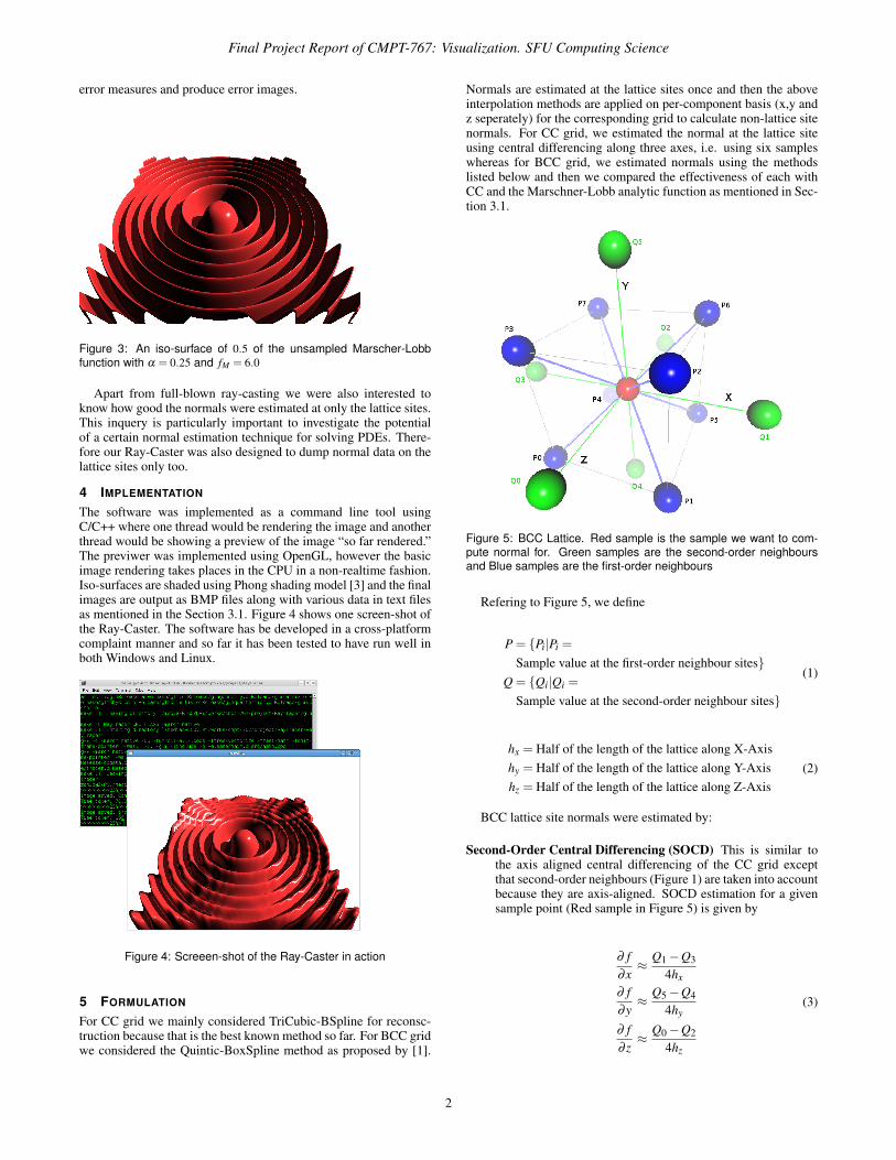
The main objective of the “Compare” mode is to compare the re-construction quality of different grids with an analytic function forwhich we chose the widely used Marschner-Lobb function [2]. Wechose α = 0.25 and fM = 6.0 for the Marschner-Lobb function andFigure 3 shows an iso-surface of 0.5 of the said unsampled function.In this mode, ray is casted into the analytic function and wheneveran iso-surface is hit, all the other grid in the system are evaluatedexactly at the same 3D point for both data value and normal. Thisdesign was adopted instead of ray-casting seperately on grids tomake sure we are comparing between the analytic function and allthe other grids exactly at the same 3D points. The actual functionvalue and normal and all the other evluated data value with normalscorresponding to the same 3D point were then dumped into a textfile. Matlab was then used to read that text file, compute various

1


error measures and produce error images.

Figure 3: An iso-surface of 0.5 of the unsampled Marscher-Lobbfunction with α = 0.25 and fM = 6.0

Apart from full-blown ray-casting we were also interested toknow how good the normals were estimated at only the lattice sites.This inquery is particularly important to investigate the potentialof a certain normal estimation technique for solving PDEs. There-fore our Ray-Caster was also designed to dump normal data on thelattice sites only too.

4 IMPLEMENTATION

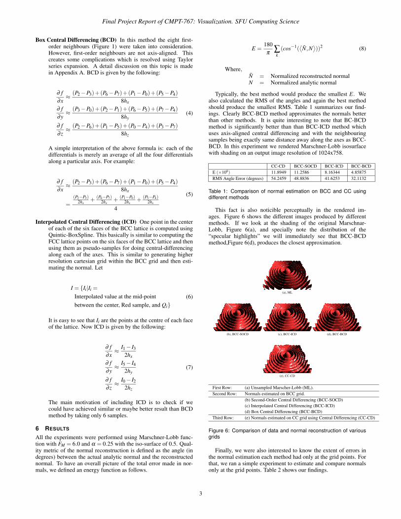
The software was implemented as a command line tool usingC/C++ where one thread would be rendering the image and anotherthread would be showing a preview of the image “so far rendered.”The previwer was implemented using OpenGL, however the basicimage rendering takes places in the CPU in a non-realtime fashion.Iso-surfaces are shaded using Phong shading model [3] and the finalimages are output as BMP files along with various data in text filesas mentioned in the Section 3.1. Figure 4 shows one screen-shot ofthe Ray-Caster. The software has be developed in a cross-platformcomplaint manner and so far it has been tested to have run well inboth Windows and Linux.

Figure 4: Screeen-shot of the Ray-Caster in action

5 FORMULATION

For CC grid we mainly considered TriCubic-BSpline for reconsc-truction because that is the best known method so far. For BCC gridwe considered the Quintic-BoxSpline method as proposed by [1].

Normals are estimated at the lattice sites once and then the aboveinterpolation methods are applied on per-component basis (x,y andz seperately) for the corresponding grid to calculate non-lattice sitenormals. For CC grid, we estimated the normal at the lattice siteusing central differencing along three axes, i.e. using six sampleswhereas for BCC grid, we estimated normals using the methodslisted below and then we compared the effectiveness of each withCC and the Marschner-Lobb analytic function as mentioned in Sec-tion 3.1.

Figure 5: BCC Lattice. Red sample is the sample we want to com-pute normal for. Green samples are the second-order neighboursand Blue samples are the first-order neighbours

Refering to Figure 5, we define

P = {Pi|Pi =

Sample value at the first-order neighbour sites}

Q = {Qi|Qi =

Sample value at the second-order neighbour sites}

(1)

hx = Half of the length of the lattice along X-Axis

hy = Half of the length of the lattice along Y-Axis

hz = Half of the length of the lattice along Z-Axis

(2)

BCC lattice site normals were estimated by:

Second-Order Central Differencing (SOCD) This is similar tothe axis aligned central differencing of the CC grid exceptthat second-order neighbours (Figure 1) are taken into accountbecause they are axis-aligned. SOCD estimation for a givensample point (Red sample in Figure 5) is given by

∂ f

∂x≈

Q1 −Q3

4hx

∂ f

∂y≈

Q5 −Q4

4hy

∂ f

∂ z≈

Q0 −Q2

4hz

(3)

2


Box Central Differencing (BCD) In this method the eight first-order neighbours (Figure 1) were taken into consideration.However, first-order neighbours are not axis-aligned. Thiscreates some complications which is resolved using Taylorseries expansion. A detail discussion on this topic is madein Appendix A. BCD is given by the following:

∂ f

∂x≈

(P2 −P3)+(P6 −P7)+(P1 −P0)+(P5 −P4)

8hx

∂ f

∂y≈

(P3 −P0)+(P2 −P1)+(P6 −P5)+(P7 −P4)

8hy

∂ f

∂ z≈

(P2 −P6)+(P1 −P5)+(P0 −P4)+(P3 −P7)

8hz

(4)

A simple interpretation of the above formula is: each of thedifferentials is merely an average of all the four differentialsalong a particular axis. For example:

∂ f

∂x≈

(P2 −P3)+(P6 −P7)+(P1 −P0)+(P5 −P4)

8hx

=

(P2−P3)2hx

+(P6−P7)

2hx+

(P1−P0)2hx

+(P5−P4)

2hx

4

(5)

Interpolated Central Differencing (ICD) One point in the centerof each of the six faces of the BCC lattice is computed usingQuintic-BoxSpline. This basically is similar to computing theFCC lattice points on the six faces of the BCC lattice and thenusing them as pseudo-samples for doing central-differencingalong each of the axes. This is similar to generating higherresolution cartesian grid within the BCC grid and then esti-mating the normal. Let

I = {Ii|Ii =

Interpolated value at the mid-point

between the center, Red sample, and Qi}

(6)

It is easy to see that Ii are the points at the centre of each faceof the lattice. Now ICD is given by the following:

∂ f

∂x≈

I1 − I3

2hx

∂ f

∂y≈

I5 − I4

2hy

∂ f

∂ z≈

I0 − I2

2hz

(7)

The main motivation of including ICD is to check if wecould have achieved similar or maybe better result than BCDmethod by taking only 6 samples.

6 RESULTS

All the experiments were performed using Marschner-Lobb func-tion with FM = 6.0 and α = 0.25 with the iso-surface of 0.5. Qual-ity metric of the normal reconstruction is defined as the angle (indegrees) between the actual analytic normal and the reconstructednormal. To have an overall picture of the total error made in nor-mals, we defined an energy function as follows.

E =180

π∑k

(cos−1(⟨

N,N⟩

))2 (8)

Where,

N = Normalized reconstructed normalN = Normalized analytic normal

Typically, the best method would produce the smallest E. Wealso calculated the RMS of the angles and again the best methodshould produce the smallest RMS. Table 1 summarizes our find-ings. Clearly BCC-BCD method approximates the normals betterthan other methods. It is quite interesting to note that BC-BCDmethod is significantly better than than BCC-ICD method whichuses axis-aligned central differencing and with the neighbouringsamples being exactly same distance away along the axes as BCC-BCD. In this experiment we rendered Marschner-Lobb isosurfacewith shading on an output image resolution of 1024x758.

CC-CD BCC-SOCD BCC-ICD BCC-BCD

E (×108) 11.8949 11.2586 8.16344 4.85875

RMS Angle Error (degrees) 54.2459 48.8836 41.6253 32.1132

Table 1: Comparison of normal estimation on BCC and CC usingdifferent methods

This fact is also noticible perceptually in the rendered im-ages. Figure 6 shows the different images produced by differentmethods. If we look at the shading of the original Marschnar-Lobb, Figure 6(a), and specially note the distribution of the“specular highlights” we will immediately see that BCC-BCDmethod,Figure 6(d), produces the closest approximation.

(a), ML

(b), BCC-SOCD (c), BCC-ICD (d), BCC-BCD

(e), CC-CD

First Row: (a) Unsampled Marscher-Lobb (ML).

Second Row: Normals estimated on BCC grid.

(b) Second-Order Central Differencing (BCC-SOCD)

(c) Interpolated Central Differencing (BCC-ICD)

(d) Box Central Differencing (BCC-BCD)

Third Row: (e) Normals estimated on CC grid using Central Differencing (CC-CD)

Figure 6: Comparison of data and normal reconstruction of variousgrids

Finally, we were also interested to know the extent of errors inthe normal estimation each method had only at the grid points. Forthat, we ran a simple experiment to estimate and compare normalsonly at the grid points. Table 2 shows our findings.

3


(b), BCC-SOCD (c), BCC-ICD (d), BCC-BCD

(e), CC-CD

First Row: (a) Unsampled Marscher-Lobb (ML).

Second Row: Normals estimated on BCC grid.

(b) Second-Order Central Differencing (BCC-SOCD)

(c) Interpolated Central Differencing (BCC-ICD)

(d) Box Central Differencing (BCC-BCD)

Third Row: (e) Normals estimated on CC grid using Central Differencing (CC-CD)

Figure 7: Comparison of data and normal reconstruction with errorimages of various grids

CC-CD BCC-SOCD BCC-ICD BCC-BCD

E (×108) 0.880199 1.11468 0.73573 0.517233

RMS Angle Error (degrees) 35.7367 40.216 32.6726 27.3947

Table 2: Comparison of normal estimation only at the grid points onBCC and CC using different methods

Clearly Table 2 is consistent with the fact that BCC-BCD ap-proximates normals better than other methods.

7 CONCLUSION

In this project we have studied some existing techniques for esti-mating normals at the lattice point of CC and BCC grids. We havealso proposed a novel approach towards estimating normals on aBCC grid which exploits the nearer eight first order neighbours.Mathematical analysis (see Appendix A) and our experiments ver-ify that the newer Box Central Differencing (BCD) technique isindeed superior. Not only this method has great potential for shad-ing volumes better but also has potential along the lines of solvingPDEs.

ACKNOWLEDGEMENTS

The authors wish to thank Usman Alim, Steven Bergner, BernhardFinkbeiner of GRUVi lab at Simon Fraser University for their re-lentless support.

A APPENDIX

A.1 BCC Box Central Differencing (BCC-BCD)

To derive the BCC-BCD method we assume a trivariate functionf (u,v,w). The Taylor series expansion upto quadratic order of thisfunction about the point (x,y,z) is given by

f (u,v,w) = f (x,y,z)+(u− x)∂ f

∂u(x,y,z)+

(v− y)∂ f

∂v(x,y,z)+

(w− z)∂ f

∂w(x,y,z)+

1

2(u− x)2 ∂ 2 f

∂u2(x,y,z)+

(u− x)(v− y)∂

∂v

∂ f

∂u(x,y,z)+

(u− x)(w− z)∂

∂w

∂ f

∂u(x,y,z)+

(v− y)(w− z)∂

∂w

∂ f

∂v(x,y,z)+

1

2(v− y)2 ∂ 2 f

∂v2( f )(x,y,z)+

1

2(w− z)2 ∂ 2 f

∂w2(x,y,z)+ . . .

(9)

Now let us define the points P = {P0,P1,P2,P3,P4,P5,P6,P7} asfollows:

P0 = f (x−hx,y−hy,z+hz)

P1 = f (x+hx,y−hy,z+hz)

P2 = f (x+hx,y+hy,z+hz)

P3 = f (x−hx,y+hy,z+hz)

P4 = f (x−hx,y−hy,z−hz)

P5 = f (x+hx,y−hy,z−hz)

P6 = f (x+hx,y+hy,z−hz)

P7 = f (x−hx,y+hy,z−hz)

(10)

Note that the point set P is exactly the same P point set of Fig-ure 5

Now let us write

S = AP0 +BP1 +CP2 +DP3 +EP4 +FP5 +GP6 +HP7 (11)

Where {A,B,C,D,E,F,G,H} are all constants

Writing Equation 9 up to cubic order and substituting Equa-tion 10 into it we can rewrite S as

4


S =(A+B+C +E +F +G+H +D) f (x,y,z)+

hx(−A+B+C−E +F +G−H −D)∂ f

∂u(x,y,z)+

hy(−A−B+C−E −F +G+H +D)∂ f

∂v(x,y,z)+

hz(A+B+C−E −F −G−H +D)∂ f

∂w(x,y,z)+

h2x

2(A+B+C +E +F +G+H +D)

∂ 2 f

∂u2(x,y,z)+

h2y

2(A+B+C +E +F +G+H +D)

∂ 2 f

∂y2(x,y,z)+

h2z

2(A+B+C +E +F +G+H +D)

∂ 2 f

∂w2(x,y,z)+

h3x

6(−A+B+C−E +F +G−H −D)

∂ 3 f

∂u3(x,y,z)+

d3y

6(−A−B+C−E −F +G+H +D)

∂ 3 f

∂v3(x,y,z)+

h3z

6(A+B+C−E −F −G−H +D)

∂ 3 f

∂w3(x,y,z)

hxhy(A−B+C +E −F +G−H −D)∂

∂v

∂ f

∂u(x,y,z)+

hxhz(−A+B+C +E −F −G+H −D)∂

∂w

∂ f

∂u(x,y,z)+

hyhz(−A−B+C +E +F −G−H +D)∂

∂w

∂ f

∂v(x,y,z)+

h2xhy

2(−A−B+C−E −F +G+H +D)

∂

∂v

∂ 2 f

∂u2(x,y,z)+

h2xhz

2(A+B+C−E −F −G−H +D)

∂

∂w

∂ 2 f

∂u2(x,y,z)+

hxh2y

2(−A+B+C−E +F +G−H −D)

∂ 2

∂v2

∂ f

∂u(x,y,z)+

hxh2z

2(−A+B+C−E +F +G−H −D)

∂ 2

∂w2

∂ f

∂u(x,y,z)+

h2yhz

2(A+B+C−E −F −G−H +D)

∂

∂w

∂ 2 f

∂v2(x,y,z)+

hyh2z

2(−A−B+C−E −F +G+H +D)

∂ 2

∂w2

∂ f

∂v(x,y,z)+

hxhyhz(A−B+C−E +F −G+H −D)∂

∂w

∂

∂v

∂ f

∂u(x,y,z)+

(12)

Now, let us try to isolate∂ f∂u

out of the above equation and forthat let us take the following:

A+B+C +E +F +G+H +D = 0, with f (x,y,z)

−A+B+C−E +F +G−H −D = 1, with∂ f∂u

−A−B+C−E −F +G+H +D = 0, with∂ f∂v

A+B+C−E −F −G−H +D = 0, with∂ f∂w

A−B+C +E −F +G−H −D = 0, with ∂∂v

∂ f∂u

−A+B+C +E −F −G+H −D = 0, with ∂∂w

∂ f∂u

−A−B+C +E +F −G−H +D = 0, with ∂∂w

∂ f∂v

A−B+C−E +F −G+H −D = 0, with ∂∂w

∂∂v

∂ f∂u

(13)

This forms a system of linear equations and the solution of theabove system is

{

A = −1

8,B =

1

8,C =

1

8,D = −

1

8,

E = −1

8,F =

1

8,G =

1

8,H = −

1

8

}

(14)

If we plug in the above solution to S, we have

S =1

2hxh2

y

∂ 2

∂v2

∂ f

∂u(x,y,z)+

1

2hxh2

z

∂ 2

∂w2

∂ f

∂u(x,y,z)+

hx∂ f

∂u(x,y,z)+

1

6h3

x

∂ 3 f

∂u3(x,y,z) (15)

Dividing both sides by hx gives

Nx =S

hx=

∂ f

∂u(x,y,z)+

1

2h2

y

∂ 2

∂v2

∂ f

∂u(x,y,z)+

1

2h2

z

∂ 2

∂w2

∂ f

∂u(x,y,z)+

1

6h2

x

∂ 3 f

∂u3(x,y,z) (16)

If f (u,v,w) has a maximum order of two, i.e. quadratic in naturewhich in turns also means if f (u,v,w) can be characterized by the

linear combination of the shifted verson of (u + v + w)2 then Nx =∂ f∂u

. This is because if

f (u,v,w) =∑i

∑j∑k

Wi jk{(u−ai)+(v−b j)+(w− ck)}2

Where, Wi jk,ai,b j,ck are all constants

(17)

then it follows

∂ 2

∂v2

∂ f

∂u(x,y,z) = 0

∂ 2

∂w2

∂ f

∂u(x,y,z) = 0

∂ 3 f

∂u3(x,y,z) = 0

But for fairly small hx we can always approximate

Nx ≈∂ f

∂u(x,y,z) ≈

S

hx

=(P2 −P3)+(P6 −P7)+(P1 −P0)+(P5 −P4)

8hx(18)

Similarly Ny,Nz can also be found using the same pattern.

5


B APPENDIX

C SOME RENDERED OUTPUT OF THE RAY-CASTER

(b), CC

(d), BCC-SOCD

(c), BCC-ICD

(e), BCC-BCD

Figure 8: Comparison of data and normal reconstruction on Carpdataset

REFERENCES

[1] A. Entezari, D. Van De Ville, and T. Moller. Practical box splines for

volume rendering on the body centered cubic lattice. IEEE Transac-

tions on Visualization and Computer Graphics, 14(2):313 – 328, 2008.

[2] S. R. Marschner and R. J. Lobb. An evaluation of reconstruction filters

for volume rendering. In R. D. Bergeron and A. E. Kaufman, editors,

Proceedings of the IEEE Conference on Visualization, pages 100–107.

IEEE Computer Society Press, Oct. 1994.

[3] B. T. Phong. Illumination for computer generated pictures. Commun.

ACM, 18(6):311–317, 1975.

[4] A. E. Usman R. Alim and T. Moller. The lattice-boltzmann method on

optimal sampling lattices. Technical report, 2008.

6

a novel approach and comparison of normal estimation...

Documents