a numerical framework for isotropic and anisotropic
TRANSCRIPT

American Institute of Aeronautics and Astronautics
1
A Numerical Framework for Isotropic and Anisotropic
Flexible Flapping Wing Aerodynamics and Aeroelasticity
Hikaru Aono*, Chang-kwon Kang
†, Carlos E. S. Cesnik
‡, and Wei Shyy
§
Department of Aerospace Engineering, University of Michigan, Ann Arbor, MI, 48105
A numerical framework is presented to simulate rigid and flexible flapping wings. The
fluid-structure interaction is realized by coupling a Navier-Stokes solver to a geometrically
nonlinear co-rotational structural solver. In the coupled fluid-structure interaction interface
the aerodynamic loading and deformed wing surface are shared by two solvers within each
time step. A remeshing method based on radial basis function is implemented to handle large
deformations, preserve grid quality, and execute economically. Flexible flapping wing
operating in both vacuum and air is considered to shed light on inertial and aerodynamic
loading-induced shape deformation. Impacts of flapping isotropic wing with single degree of
freedom rotation on aerodynamic force generation are presented for Re= 1.5×10³ and k=
0.56. The results indicate: 1) the flexibility-induced pitching angle promotes thrust
generation, and 2) the increase of wing velocity due to large bending motion enhances
aerodynamic force by increasing pressure differences. For a wing of anisotropic mechanical
properties, highly three-dimensional wing deformation is observed when the wing
accelerates or decelerates in absent of aerodynamic loadings.
Nomenclature
= aspect ratio, [1]
= element extensional stiffness matrix [Pa m]
= mean wing span [m]
= membrane-bending coupling stiffness matrix [Pa m
2]
= lift coefficient, [1]
= mean chord length [m]
= thrust coefficient, [1]
= bending stiffness matrix [Pa m
3]
= Young’s modulus of an isotropic material [Pa]
= Young’s modulus of an orthotropic material in the direction [Pa]
= Young’s modulus of an orthotropic material in the direction [Pa]
= motion frequency [1/s]
= distributed external force [N]
= Shear modulus of an orthotropic material in the plane [Pa]
= thickness of a plate [m]
= reduced frequency, [1]
= mesh refinement factor [1]
= number of boundary nodes with specified displacements [1]
= number of nodes on structural mesh [1]
= number of internal nodes [1]
* Post- doctoral Research Fellow, Department of Aerospace Engineering, University of Michigan, AIAA Member
†Graduate Student Research Assistant, Department of Aerospace Engineering, University of Michigan, AIAA
Student Member ‡ Professor, Department of Aerospace Engineering, University of Michigan, AIAA Associate Fellow
§ Clarence L. “Kelly” Johnson Collegiate Professor and Chair, Department of Aerospace Engineering, University of
Michigan, AIAA Fellow.
28th AIAA Applied Aerodynamics Conference28 June - 1 July 2010, Chicago, Illinois
AIAA 2010-5082
Copyright © 2010 by the American Institute of Aeronautics and Astronautics, Inc. All rights reserved.
American Institute of Aeronautics and Astronautics
2
= force resultant [N]
= moment resultant [N m]
= pressure [Pa]
= component of reduced stiffness matrix at th
layer
= support radius of compact radial basis functions [m]
= semi-span [m]
= Reynolds number, [1]
= wing planform area [m2]
= Strouhal number, [1]
= time [s]
= period of flapping motion = [s]
= mean wing tip velocity, [m/s]
= velocity vector [m/s]
= volume of a cell [1]
= position vector [m]
= displacement vector of a structural node at time step of fsi-iteration
[m]
= position vector on the aerodynamic volume node [m]
= displacement vector on the aerodynamic volume node [m]
= position vector on the boundary node [m]
= displacement vector on the boundary node [m]
= weight coefficients [m]
= polynomial belonging to the aerodynamic volume node [1]
= membrane strains in the mid-surface of a plate [1]
= flexural strains in the mid-surface of a plate [1]
= Poisson’s ratio [1]
= dynamic viscosity of fluid [Pa s]
= effective stiffness of flat plate,
[1]
= ply angle of unidirectional fiber [degree/radian]
= density ratio, [1]
= density of fluid [kg m-3
]
= density of structure [kg m-3
]
= radial basis function [1]
= stroke angle [degree/radian]
= full stroke amplitude [degree/radian]
= coupling matrix from the aerodynamic boundary nodes to volume nodes [1]
= motion angular frequency [1/s]
= out-of-plane displacement of an isotropic plate [m]
= vertical tip deflection [m]
= distance from the mid-surface of a plate at th layer [m]
= vertical tip location/position [m]
= normalized variable [1]
I. Introduction
ICRO air vehicles (MAVs) are flyers with maximum dimensions of 1.5×10⁻¹
m that can lead to revolutionary
improvements in remote sensing and information gathering capabilities both in military as well in civilian
applications. As the size of the flyer is orders of magnitudes smaller than a conventional aircraft, the fluid dynamics,
hence the lift generation, and the flight control governing a MAV change considerably1, 2
: Smaller sizes and lower
flight speeds lead to lower Reynolds numbers, and higher sensitivity to wind gust effects. Moreover, wings are in
general flexible and deform during flight. Consequently, design of a high performance and robust MAV become a
highly nonlinear complex process that requires solid understanding of aerodynamics, structural dynamics, control,
and interactions of these.
M

American Institute of Aeronautics and Astronautics
3
In the nature, biological flyers, such as insects and birds, share similar dimensions and flight characteristics as
MAVs1. The physics exhibited by these biological flyers thus have potential to be applied in MAV design
1.
Unsteady aerodynamic mechanisms such as the generation of a leading edge vortex (LEV), wing-wake interaction,
and three-dimensional flow features, such as tip vortex-vortex interactions, all contribute significantly to affect the
aerodynamic force generation2. Another remarkable mechanism that the biological flyers seem to be using is the
wing flexibility. Studies have been performed to shed light on the interplay between the structural flexibility and the
resulting aerodynamic forces3- 6
. For example, Combes and Daniel7,8
have shown that a variety of insects exhibit
anisotropy in their wing structures based on static response tests. The spanwise flexural rigidity was 1 or 2 orders of
magnitudes larger than the chordwise flexural rigidity. Recent experimental and numerical4 show that the chordwise
flexibility affects the redistribution of the resulting aerodynamic forces in the lift and the thrust directions. For
example, if the airfoil shape undergoes deformation then the camber of the airfoil may change, leading to an
effective geometry of the airfoil, and combined with the pitching angle the direction of the net force can be adjusted
in favor of the thrust generation. Furthermore, for a range of spanwise flexibility, deformed airfoil shapes along the
spanwise direction and the correct direction of the motion are seen to enhance the thrust of a plunging wing9,10
. The
fluid-structure density ratio affects the thrust generation: Zhu11
showed numerically that the thrust and the
propulsive efficiencies increased for a plunging chordwise flexible airfoil in water than immersed in air. Hence it is
seen that the flexibility, including the density ratio can be utilized to control resulting aerodynamic forces. However
the precise underlying physics of aeroelastic coupling for flapping wings and its applicability to the MAV designs
are yet to be understood. Shyy et al.2 offer an extensive review on the aerodynamics of rigid and flexible wings.
Recently, systematic methodologies of experiment have been developed to optimize thrust generated by single
degree-of-freedom (DOF) flapping wing via variation of wing structures12
. In these studies, several combinations of
flapping wing frequency, amplitude, and wing structure are examined. The conclusion made from the experimental
studies is that for flapping wing structure optimization in hovering flight on size scale of humming birds or insects,
each wing structure must be tailored according to a certain kinematics (with a desired flapping frequency and
amplitude) and optimized for performance values such as either lift by drag or flight efficiency. Scaling parameters
resulting from dimensional analysis and by non-dimensionalizing the governing equations by relevant physical
variables, often give qualitative characteristics of the model as well as the requirement for dynamic similarity of the
flow13
. Depending on the type of the model and the governing equations the resulting set of scaling parameters may
vary. Shyy et al.1, 2
have considered the Navier-Stokes equations with out-of-plane motion of an isotropic plate,
Ishihara et al.5,14
, the Navier-Stokes equations and the wing structure as a linear isotropic elastic body to study the
flexibility effect on wing pitch changes in dipteran flapping flight, and Lentink and Dickinson15
transformed the
Navier-Stokes equation in the wing-fitted frame of reference and focused on the rotational motion of the wing. The
scaling parameters related to the unsteady aerodynamics, such as the Reynolds number, the Strouhal number, or the
reduced frequency have been explored previously1,2
, still the parameter-space involving the scaling parameters for
the fluid-structure interaction needs to be mapped out in a systematic fashion to understand the role of flexibility on
flapping wing force generation.
Different levels of fidelity and diverse numerical algorithms, depending on the objective of the study and
accuracy and cost of the computations, can be incorporated into a numerical framework of flexible flapping wing
simulations. High-fidelity framework can be used to evince the rich and complex physics behind flexible flapping
wing aerodynamics, while a low-fidelity model can be used for quick yet reliable design optimization of a complex
and multi-dimensional design space. The aeroelastic coupling can be based on a time-domain partitioned process
where the interaction between the fluid and the solid fields occurs at a shared boundary iteratively at a given time
step. An advantage is that for the solutions of both fields, which are described by different nonlinear partial
differential equations, well-established solvers can be used. Tang et al.16
, Chimakurti et al.10, 17
, and Aono et al.4, 18
have coupled an in-house finite-volume based Navier-Stokes solver to a beam model16
, a commercial nonlinear
finite-element solver, MSC.Marc10
, a geometrically nonlinear active beam solver10
, and a co-rotational shell finite
element model17,4,18
, respectively. Furthermore, Gordnier et al.19
coupled an in-house high-order Navier-Stokes
solver to a geometrically nonlinear active beam solver, McClung et al.20
developed the OVERFLOW Navier-Stokes
solver to a modal representation of two-dimensional beam, and Stanford et al.21
combined a two-dimensional quasi-
steady blade element model to a nonlinear co-rotational beam model.
Some of the numerical challenges associated with aeroelastic coupling of highly deformable three-dimensional
flapping wings are that large number of cells are required to resolve the necessary flow field phenomena such as
vorticity generation near the wing as well as convection and diffusion of large scale vortical structures away from
the wing and that large flapping amplitudes and deformations lead to large mesh deformations that require
numerically robust and efficient remeshing algorithms. To obtain the three-dimensional flow solutions with the
number of cells in the orders of O(106) a Navier-Stokes equations solver is often parallelized, which introduces

American Institute of Aeronautics and Astronautics
4
obvious implementation challenges for the problems involving moving meshes: how to efficiently communicate
information between multiple processors about the displacements stored in other processors to remesh the grid; and
how to provide interface for the communication for the fluid-structure interaction involving two distinct solvers,
where one or both solvers are parallelized. Two strategies have been studied for unstructured grids. In the first
category the computational mesh is considered as an elastic solid, where the new nodal displacements are obtained
by solving the structural dynamics equations. For example, Stein and Tezduyar22
proposed to solve the linear
elastostatics equations with a stiffening factor to reduce the volumetric distortion to maintain the mesh quality in
finite element formulation. Smith and Wright23
recast the linear elastostatics equations in finite-volume
discretization, which involves similar terms as the Navier-Stokes equations, so that the remeshing algorithm could
be implemented based on the readily available momentum equation solver as a template. In the second category the
nodal displacements are interpolated using Radial Basis Functions (RBF) based on the displacements given at the
boundary conditions, either prescribed or from the structural dynamics solver. This method, as the cell connectivity
information is not required, can be applied to structured and unstructured meshes and is seen to keep initial mesh
qualities well and efficiently24-27
.
Chimakurthi et al.10
have presented a computational framework capable of computing flexible flapping wing
aerodynamics and aeroelasticity. They have detailed fluid and structural solvers as well as the coupling strategies.
Aono et al.4 have further developed the techniques and investigated the dynamic characteristics associated with
spanwise flexibility of a plunging wing. Chordwise flexibility of a plunging wing is discussed in Shyy et al.2. The
computational framework is restricted to isotropic wing structures. In the present paper, we have advanced the
computational capabilities presented in Ref 10. Specifically, we have incorporated an unstructured grid Navier-
Stokes solver and an anisotropic structural solver. The interface between fluid and structure solvers is based on that
reported in Ref 10. Furthermore, new remeshing techniques, similar to that reported by De Boer et al.24
and Rendall
and Allen25-27
, have been developed and tested. The added capabilities can handle a variety of wing structures with
large flapping translation and rotation. In order to shed light on the role of inertial and aerodynamic loading-induced
shape deformation associated with a flapping flexible wing, wings operating in both vacuum and air are considered.
To account for the anisotropic nature of wing structures, a composite structural model is implemented based on the
classical laminate plate theories39
. Structural dynamic response of flapping anisotropic wing models in vacuum are
presented and compared with the experimental data12
. Furthermore, a remeshing method using the RBF interpolation
is presented that is able to efficiently deform large number of nodes under large wing movements, while keeping the
initial mesh qualities. The fluid flow obtained by using a finite-volume pressure-based Navier-Stokes solver and the
structural dynamics solver uses the finite element method with an optimal membrane element and a discrete
Kirchhoff triangle plate bending element in a co-rotational formulation to effectively simulate a thin flexible wing17
.
In the coupled fluid-structure interaction interface the aerodynamic loading and deformed wing surface is shared by
two solvers within each time step. The relevance of this framework is three-fold. The computed fluid flow field and
the structural response can be studied to understand the nonlinear coupled field problem for flapping wing flyers,
also these results can function as a validation for lower order tools or experimental results. Moreover, this
framework can serve as a tool to construct a quick and reliable design guideline for MAV applications.
II. Methodology
A. Computational fluid dynamics
1. Governing equations
The governing equations for the fluids are unsteady three-dimensional Navier-Stokes equations with constant
density and viscosity shown in Eqs. (1) and (2),
(1)
(2)
where is the velocity vector, is the position vector, is the time, is the pressure, is the fluid velocity, and
the viscosity of the fluid. The Eqs (1) and (2) are solved with in-house codes18, 28, 29
, which are three-dimensional
pressure-based finite-volume solvers. The parallelization is realized using the Loci framework30
. It employs implicit
first or second order time stepping and treats convection terms using the second order upwind-type scheme28, 31, 32
,
American Institute of Aeronautics and Astronautics
5
pressure and viscous terms using second order schemes. The system of equations resulting from the linearized
momentum equations are handled with the symmetric Gauss-Seidel33
solver which has relatively low memory
requirements. The pressure correction equation28, 35
is solved with the GMRES linear solver with Jacobi
preconditions provided by PETSc35
. The geometric conservation law, a necessary consideration in domains with
moving boundaries, is satisfied36, 37
. The mesh deformations are realized using either Radial Basis Function (RBF)
or thin plate spline interpolations16-18
.
2. Remeshing
De Boer et al.24
and Rendall and Allen25-27
have shown the effectiveness of using RBF interpolation method to
remesh the unstructured grids. There are two distinctive advantages: i) Connectivity information is unnecessary for
the RBF interpolation method, that means any arbitrary order of nodal information will result in the same mesh.
However, ordering the nodes based on the distances between the nodes will make the linear system more diagonally
dominant for the compact RBFs24
, which will reduce the computational time. ii) The resulting mesh keeps the
original mesh quality, especially the orthogonality near the moving boundary surface24, 25
which is important in
viscous fluid computation where the cells are usually stretched and clustered to capture small length scale flow
phenomena.
Given the boundary displacement vector at the node , with the position either on the aerodynamic
surface mesh of a flexible body, or any other prescribed boundary surface, for instance zero displacements at the
tunnel wall, the displacement vector, , of a node , with the position , of the aerodynamic volume mesh with
respect to the initial grid, is given by Eq. (3) with summation of repeated indices as
(3)
where index represents the three components in three-dimensional space, is the coupling matrix from the
aerodynamic surface nodes to the aerodynamic volume nodes given as
with being the Euclidean distance measure acting on the index , is a radial basis function, and is a
polynomial. If the radial function is conditionally positive definite, and is a linear polynomial, then a unique
remeshing will result24, 38
. In the current study a linear polynomial will be used:
For remeshing the compact RBF constructed by Wendland38
will be used in the current study motivated by
the previous results24, 25, 38
that showed it to be computationally efficient while being able to retain the mesh
qualities, given by Eq. (4) as
(4)
where is the support radius of this compact function. As the support radius increases a node acquires more
information about the displacements of neighboring nodes, leading to better approximation. On the other hand if the
support radius is small the resulting linear system will be sparse, hence the computational cost would decrease.
However if is too small, negative jacobian or volume of a cell might occur. All RBFs, compact and global, listed
in Ref. 24 are available in the current framework for interpolation purposes.
The unknowns in Eq. (3) are the weight coefficients, ( ), and the polynomial
coefficients, , that can be solved by the requirements that the prescribed nodal displacements must be recovered
by the RBF interpolation at these nodes, i.e.,
and the additional requirement for unique solution38
,
American Institute of Aeronautics and Astronautics
6
where is a summation vector that sums all elements along , the zero vector over the index , and the zero
matrix over the index . In vector notation the resulting linear system is shown in Eq. (5) and is exactly the same as
found in Refs 24, 38:
(5)
with for each index
,
,
, ,
.
This linear system is solved using PETSc’s GMRES iterative solver with Jacobian preconditioner using multiple
processors.
To capture the three-dimensional flow phenomena the number of cells is typically in the order of millions. To
enhance the computational speed the fluid-solver is parallelized using MPI where the computational domain is
decomposed optimally for the computation of velocity and pressure fields. This implies that the boundary nodes on
the moving surfaces are randomly distributed among the processors. To implement the RBF interpolation remeshing
method efficiently in parallel the following steps are taken by noting that the nodal coordinates on the boundary
surfaces, , stay stationary in time:
1. Preprocessing step:
a. : identify the local nodes on the boundary surfaces. Using ALLGATHER operation
assemble and distribute the coordinates of all nodes on the boundary surfaces into a matrix .
b. : iterate over the local nodes on the boundary surface
and by computing the distances to all elements in construct the local partition of the system
matrix having a sparse matrix structure provided by PETSc.
2. Remeshing:
a. : solve the linear system to obtain the weight and the polynomial coefficients
locally. Using the ALLGATHER operation, distribute the coefficients globally.
b. : Compute the nodal displacements for all volume nodes by applying
Eq. (3).
Since the assembly of the system matrix is performed before the time integration begins, and the parallel
communication during the computation is only needed for the linear solver and for the ALLGATHER operation of
the coefficients, and , this method is suitable for parallelization. Further improvements can be obtained by
using the Schur-complement techniques which involve the inversion of has the potential to accelerate the
remeshing process since is a positive-definite symmetric matrix so that well-known iterative solvers can be
used such as PCG, and during the time integration only matrix multiplications are needed to obtain the new
displacements for the volume nodes25
.
B. Structural dynamics
The nonlinear structural dynamics are solved using a flexible multi-body type finite element analysis of a
flapping wing using triangular facet shell elements. The rigid-body motions are prescribed in the global frame of
reference in addition to a co-rotational framework to account for the geometric nonlinearities. By applying the co-
rotational frame transformations the motion of an element is decomposed into the rigid-body motion part and the
pure deformation part. By using the linear elasticity theory for the latter part, the co-rotational formulation can
efficiently solve for the structural dynamics with small strains, yet large rotations. A linear combination of an
optimal membrane element and a discrete Kirchhoff triangle plate bending element is employed for the elastic

American Institute of Aeronautics and Astronautics
7
stiffness of a shell element. Full details of this algorithm can be found in Ref. 17. For example, the governing
equations related to out-of-plane displacement of an isotropic flat plate may be given by Eq (6),
(6)
where is the displacement in the direction, is the density of the flat plate, is the thickness of the plate,
is the Young’s modulus of the material, is the Poisson’s ratio of the plate, and the distributed transverse load on
the plate.
To extend the isotropic structural model to an anisotropic structural model, extension stiffness, membrane-
bending coupling stiffness, and bending stiffness are constructed based on the classical laminate theories39
and the
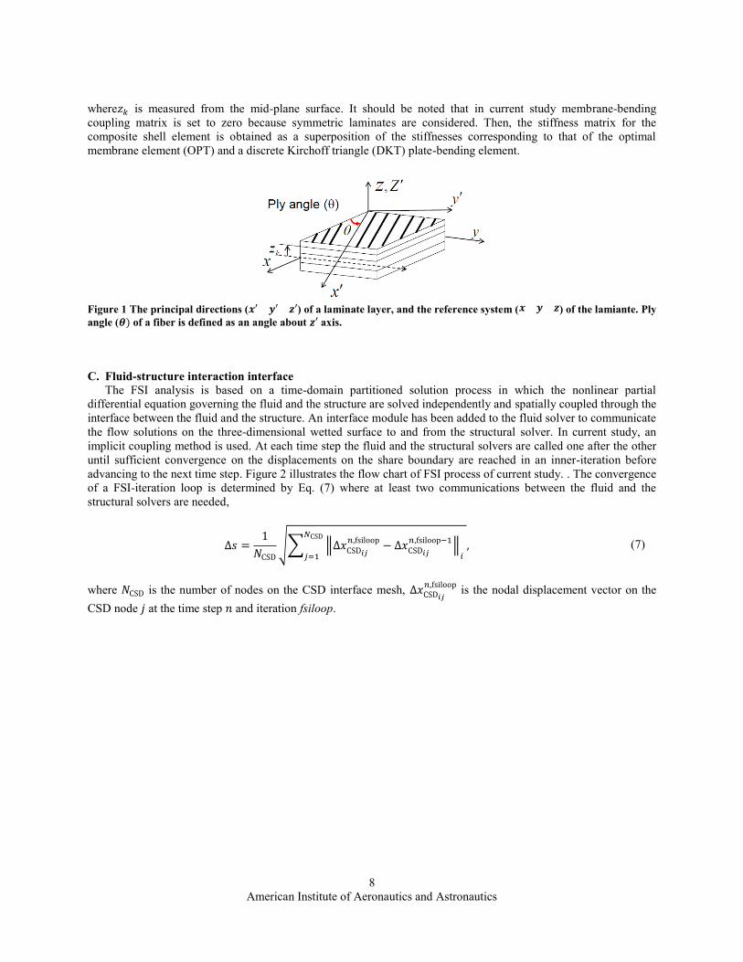
global stiffness matrix is assembled from both isotropic and orthotropic materials. A layer of unidirectional material
is considered with directions ( ), the plane ( ) being identified with the plane of the layer and the
direction with the direction of fibers as shown in Figure 1. In order to characterize the elastic properties of a layer,
expressing them in the reference axes ( of the laminate, the direction of the fibers making an angle with
the direction . This reference system is usually referred to as the system ( ). The relationship between the
off-axis reduced stiffness constants and those written in terms of the principal axes only bring in 1, 2, and 6
components of the stresses and strains. The reduced stiffness constants of a unidirectional or orthotropic composite,
off its principal directions may be written as:
where
,
,
, and
respectively. The
force-strain relationship for a thin laminate plate based the classical laminate theory39
is
where
and
are the membrane and flexural strains in the mid-surface of the plate.
and are the force resultants and moment resultants, respectively. , and
are the extensional stiffness matrix, membrane-bending coupling stiffness matrix, and bending stiffness matrix,
respectively39
:
American Institute of Aeronautics and Astronautics
8
where is measured from the mid-plane surface. It should be noted that in current study membrane-bending
coupling matrix is set to zero because symmetric laminates are considered. Then, the stiffness matrix for the
composite shell element is obtained as a superposition of the stiffnesses corresponding to that of the optimal
membrane element (OPT) and a discrete Kirchoff triangle (DKT) plate-bending element.
Figure 1 The principal directions ( ) of a laminate layer, and the reference system ( ) of the lamiante. Ply
angle ( of a fiber is defined as an angle about axis.
C. Fluid-structure interaction interface
The FSI analysis is based on a time-domain partitioned solution process in which the nonlinear partial
differential equation governing the fluid and the structure are solved independently and spatially coupled through the
interface between the fluid and the structure. An interface module has been added to the fluid solver to communicate
the flow solutions on the three-dimensional wetted surface to and from the structural solver. In current study, an
implicit coupling method is used. At each time step the fluid and the structural solvers are called one after the other
until sufficient convergence on the displacements on the share boundary are reached in an inner-iteration before
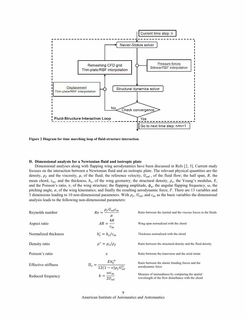
advancing to the next time step. Figure 2 illustrates the flow chart of FSI process of current study. . The convergence
of a FSI-iteration loop is determined by Eq. (7) where at least two communications between the fluid and the
structural solvers are needed,
(7)
where is the number of nodes on the CSD interface mesh,
is the nodal displacement vector on the
CSD node at the time step and iteration fsiloop.
American Institute of Aeronautics and Astronautics
9
Figure 2 Diagram for time marching loop of fluid-structure interaction.
D. Dimensional analysis for a Newtonian fluid and isotropic plate
Dimensional analyses along with flapping wing aerodynamics have been discussed in Refs [2, 3]. Current study
focuses on the interaction between a Newtonian fluid and an isotropic plate. The relevant physical quantities are the
density, and the viscosity, , of the fluid; the reference velocity, , of the fluid flow; the half span, , the
mean chord, , and the thickness, , of the wing geometry; the structural density, , the Young’s modulus, ,
and the Poisson’s ratio, , of the wing structure; the flapping amplitude, , the angular flapping frequency, , the
pitching angle, , of the wing kinematics; and finally the resulting aerodynamic force, . There are 13 variables and
3 dimensions leading to 10 non-dimensional parameters. With , , and as the basis variables the dimensional
analysis leads to the following non-dimensional parameters:
Reynolds number
Ratio between the inertial and the viscous forces in the fluids
Aspect ratio
Wing span normalized with the chord
Normalized thickness Thickness normalized with the chord
Density ratio Ratio between the structural density and the fluid density
Poisson’s ratio Ratio between the transverse and the axial strain
Effective stiffness
Ratio between the elastic bending forces and the aerodynamic force
Reduced frequency
Measure of unsteadiness by comparing the spatial wavelength of the flow disturbance with the chord
American Institute of Aeronautics and Astronautics
10
Strouhal number Ratio between the flapping speed and the reference velocity
(effective) angle of attack Curvature of the streamlines leading to pressure changes on the wing surface
Force coefficient
Aerodynamic force normalized with the dynamic pressure
and the wing surface area
If the reference velocity, , is chosen as the velocity scale, inverse of the motion frequency, , as the time
scale, and the mean chord, , as the length scale, the governing equations Eqs (2) and (6), and the motion
kinematics typically given as
(8)
where is the instantaneous flapping angle, the flapping amplitude, and the motion angular frequency, are
normalized as, see also Ref 2,
The non-dimensional variables that appear in the governing equation for the wing structures apart from the
reduced frequency are , , and . The instantaneous lift and thrust coefficients are defined as
where is the planform area of the wing, is the lift, and the thrust, such that for the resulting force, , we have
and .
III. Results and Discussions
A. Remeshing: rigidly moving flat plate in a square box
To assess the performance in terms of the mesh qualities, and domain scalability of the RBF interpolation
remeshing method, two test cases previously reported by Stein et al. 22
and Smith and Wright23
are computed. The
initial mesh consists of a computational domain in a square shape with length of two and a two percent thick flat
plate of chord length one in the center of the domain, see Figure 3. In all solutions shown in the current study the
new mesh is obtained after one time step. For the RBF the Wendland’s C2 polynomial is used with a support radius
of 2.0. The linear solver converged to the imposed absolute tolerance level of 1.0×10⁻³⁰
. In the first case the flat plate
is rotated 60 deg around its mid-chord point of the plate. The order of this angle corresponds to typical flapping
angle amplitudes1. In the second case the flat plate translates half chord length upwards. Note that the mesh is three-
dimensional with unit span length with one cell in spanwise direction to simulate two-dimensional fluid flow in a
three-dimensional fluid solver. This doubles the number of grid nodes from the two-dimensional situation.
American Institute of Aeronautics and Astronautics
11
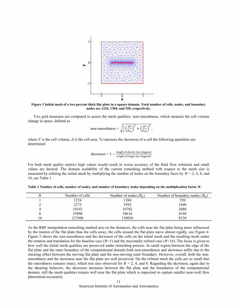
Figure 3 Initial mesh of a two percent thick flat plate in a square domain. Total number of cells, nodes, and boundary
nodes are 1224, 1384, and 520, respectively.
Two grid measures are computed to assess the mesh qualities: non-smoothness, which measure the cell volume
change in space, defined as
non-smoothness =
where is the cell volume, is the cell area. To measure the skewness of a cell the following quantities are
determined
skewness =
For both mesh quality metrics high values would result in worse accuracy of the fluid flow solutions and small
values are desired. The domain scalability of the current remeshing method with respect to the mesh size is
measured by refining the initial mesh by multiplying the number of nodes on the boundary faces by = 2, 4, 8, and
16, see Table 1.
Table 1 Number of cells, number of nodes, and number of boundary nodes depending on the multiplication factor .
Number of cells Number of nodes ( ) Number of boundary nodes ( )
1 1224 1384 520
2 3272 3592 1040
4 10142 10782 2080
8 35896 34616 4160
16 127496 130056 8320
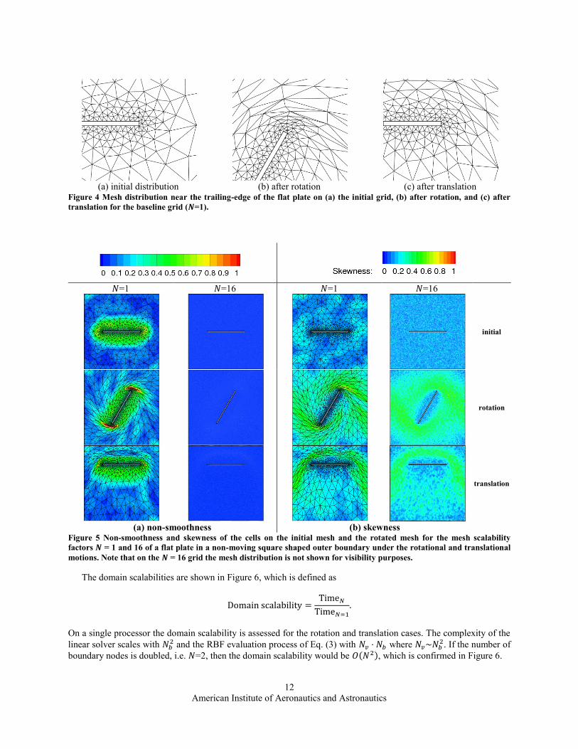
As the RBF interpolation remeshing method acts on the distances, the cells near the flat plate being more influenced
by the motion of the flat plate than the cells away, the cells around the flat plate move almost rigidly, see Figure 4.
Figure 5 shows the non-smoothness and the skewness of the cells on the initial mesh and the resulting mesh under
the rotation and translation for the baseline case ( =1) and the maximally refined case ( =16). The focus is given to
how well the initial mesh qualities are preserved under remeshing process. In small region between the edge of the
flat plate and the outer boundary of the computational domain both non-smoothness and skewness suffer due to the
shearing effect between the moving flat plate and the non-moving outer boundary. However, overall, both the non-
smoothness and the skewness near the flat plate are well preserved. On the refined mesh the cells are so small that
the smoothness remains intact, which was also observed for = 2, 4, and 8. Regarding the skewness, again due to
the shearing behavior, the skewness increases between the flat plate and the boundaries of the computational
domain, still the mesh qualities remain well near the flat plate which is important to capture smaller near-wall flow
phenomena accurately.
American Institute of Aeronautics and Astronautics
12
(a) initial distribution (b) after rotation (c) after translation
Figure 4 Mesh distribution near the trailing-edge of the flat plate on (a) the initial grid, (b) after rotation, and (c) after
translation for the baseline grid ( =1).
=1 =16 =1 =16
initial
rotation
translation
(a) non-smoothness (b) skewness Figure 5 Non-smoothness and skewness of the cells on the initial mesh and the rotated mesh for the mesh scalability
factors = 1 and 16 of a flat plate in a non-moving square shaped outer boundary under the rotational and translational
motions. Note that on the = 16 grid the mesh distribution is not shown for visibility purposes.
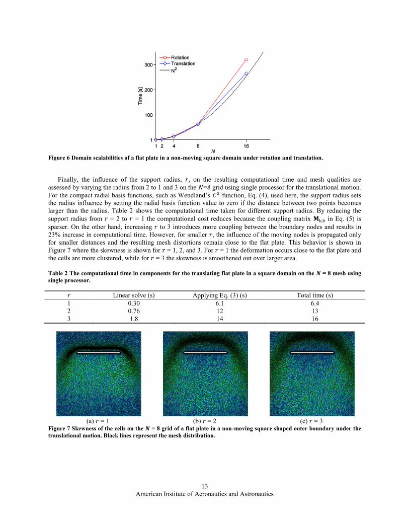
The domain scalabilities are shown in Figure 6, which is defined as
On a single processor the domain scalability is assessed for the rotation and translation cases. The complexity of the
linear solver scales with and the RBF evaluation process of Eq. (3) with where
. If the number of
boundary nodes is doubled, i.e. =2, then the domain scalability would be , which is confirmed in Figure 6.
American Institute of Aeronautics and Astronautics
13
Figure 6 Domain scalabilities of a flat plate in a non-moving square domain under rotation and translation.
Finally, the influence of the support radius, , on the resulting computational time and mesh qualities are
assessed by varying the radius from 2 to 1 and 3 on the =8 grid using single processor for the translational motion.
For the compact radial basis functions, such as Wendland’s function, Eq. (4), used here, the support radius sets
the radius influence by setting the radial basis function value to zero if the distance between two points becomes
larger than the radius. Table 2 shows the computational time taken for different support radius. By reducing the
support radius from = 2 to = 1 the computational cost reduces because the coupling matrix in Eq. (5) is
sparser. On the other hand, increasing to 3 introduces more coupling between the boundary nodes and results in
23% increase in computational time. However, for smaller , the influence of the moving nodes is propagated only
for smaller distances and the resulting mesh distortions remain close to the flat plate. This behavior is shown in
Figure 7 where the skewness is shown for = 1, 2, and 3. For = 1 the deformation occurs close to the flat plate and
the cells are more clustered, while for = 3 the skewness is smoothened out over larger area.
Table 2 The computational time in components for the translating flat plate in a square domain on the = 8 mesh using
single processor.
Linear solve (s) Applying Eq. (3) (s) Total time (s)
1 0.30 6.1 6.4
2 0.76 12 13
3 1.8 14 16
(a) = 1 (b) = 2 (c) = 3
Figure 7 Skewness of the cells on the = 8 grid of a flat plate in a non-moving square shaped outer boundary under the
translational motion. Black lines represent the mesh distribution.

American Institute of Aeronautics and Astronautics
14
B. A rigid rectangular wing prescribed with plunging excitation in free-stream at = 3.0×10⁴ and = 0.20
A rectangular wing prescribed with prescribed pure plunging excitation is simulated and compared with previous
experimental study9. The computational result is obtained using the parallel version NS solver with radio basis
function interpolation remeshing method. A schematic of the computational setup is the same as Refs. 4 and 8 and is
shown in Figure 8. The computational wing model has semi-span length of 0.3 m and a chord of = 0.1 m. A C-O
type grid around a NACA0012 wing of aspect ratio 6 is used (Figure 8 (b)). The number of grid points is 120×56×60
in the tangential, radial, and spanwise directions, respectively. The grid refinement and time step sensitivity analyses
have been performed to identify a suitable grid configuration in terms of the number of points, and the time step
increment in Ref. 4.
(a) Overview of grid topology and domain size (b) wing grid
Figure 8 Computational setup for a rectangular wing prescribed with pure plunging excitation. Purple plane indicates
symmetrical plane. (a) Overall grid topology, (b) near wing. The direction of free-stream is -axis. The wing plunges in
direction.
As to the prescribed wing motion, the leading edge of the wing root is actuated by a sinusoidal plunge
displacement profile. The amplitude and frequency of plunging motion is 0.175 and 1.74 Hz. For the boundary
conditions at the inlet, the free-stream velocity of 0.3 ms-1
is prescribed, and for the outlet, the pressure is set to zero.
A no-slip condition on the flow velocity is assigned to the wing surface. The nodes on the outer boundary surfaces
are fixed in space and time. For the support radius of the radio basis function 0.5 is chosen which is of the same
order of magnitude but larger than the half span length of 0.3. Because both the boundary nodes on the outer
boundary surfaces with zero displacements and the prescribed wing displacements construct the coupling matrix
in Eq. (5) the computational cost to remesh consist about 55% of the total computational time. A simple
method to increase the computational efficiency is presented in the section III A. The computation is run for
approximately 10 cycles (i.e. 5100 time steps) using 16 Intel® Xeon® E5540 (8M Cache, 2.53 GHz, 5.86 GT/s
Intel® QPI) processors. Per time step, the linear solver took 20 seconds to solve the linear system for the remeshing,
and 17 seconds on the slowest processor to apply Eq. (3).
American Institute of Aeronautics and Astronautics
15
(a-1) at mid-span: current study (b-1) at mid-span: experiment
(a-2) near tip: current study (b-2) near tip: experiment
(a-3) at mid-span: current study (b-3) at mid-span: experiment9
(a-4) near tip: current study (b-4) at near tip: experiment
9
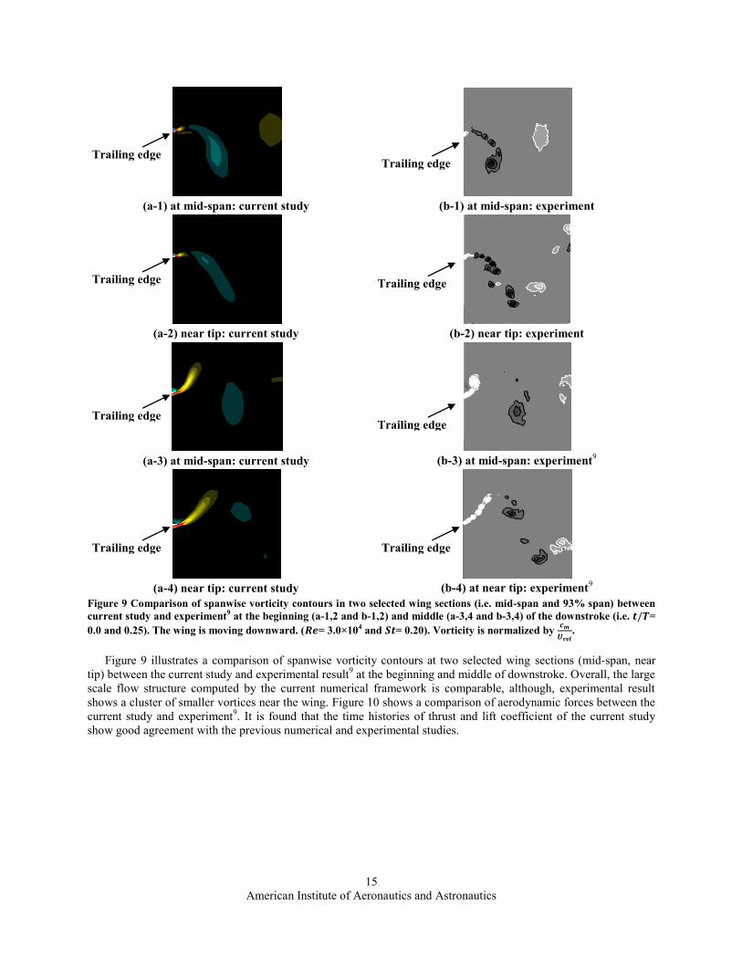
Figure 9 Comparison of spanwise vorticity contours in two selected wing sections (i.e. mid-span and 93% span) between
current study and experiment9 at the beginning (a-1,2 and b-1,2) and middle (a-3,4 and b-3,4) of the downstroke (i.e. =
0.0 and 0.25). The wing is moving downward. ( = 3.0×10⁴ and = 0.20). Vorticity is normalized by
.
Figure 9 illustrates a comparison of spanwise vorticity contours at two selected wing sections (mid-span, near
tip) between the current study and experimental result9 at the beginning and middle of downstroke. Overall, the large
scale flow structure computed by the current numerical framework is comparable, although, experimental result
shows a cluster of smaller vortices near the wing. Figure 10 shows a comparison of aerodynamic forces between the
current study and experiment9. It is found that the time histories of thrust and lift coefficient of the current study
show good agreement with the previous numerical and experimental studies.
Trailing edge
Trailing edge
Trailing edge
Trailing edge
Trailing edge
Trailing edge
Trailing edge
Trailing edge
American Institute of Aeronautics and Astronautics
16
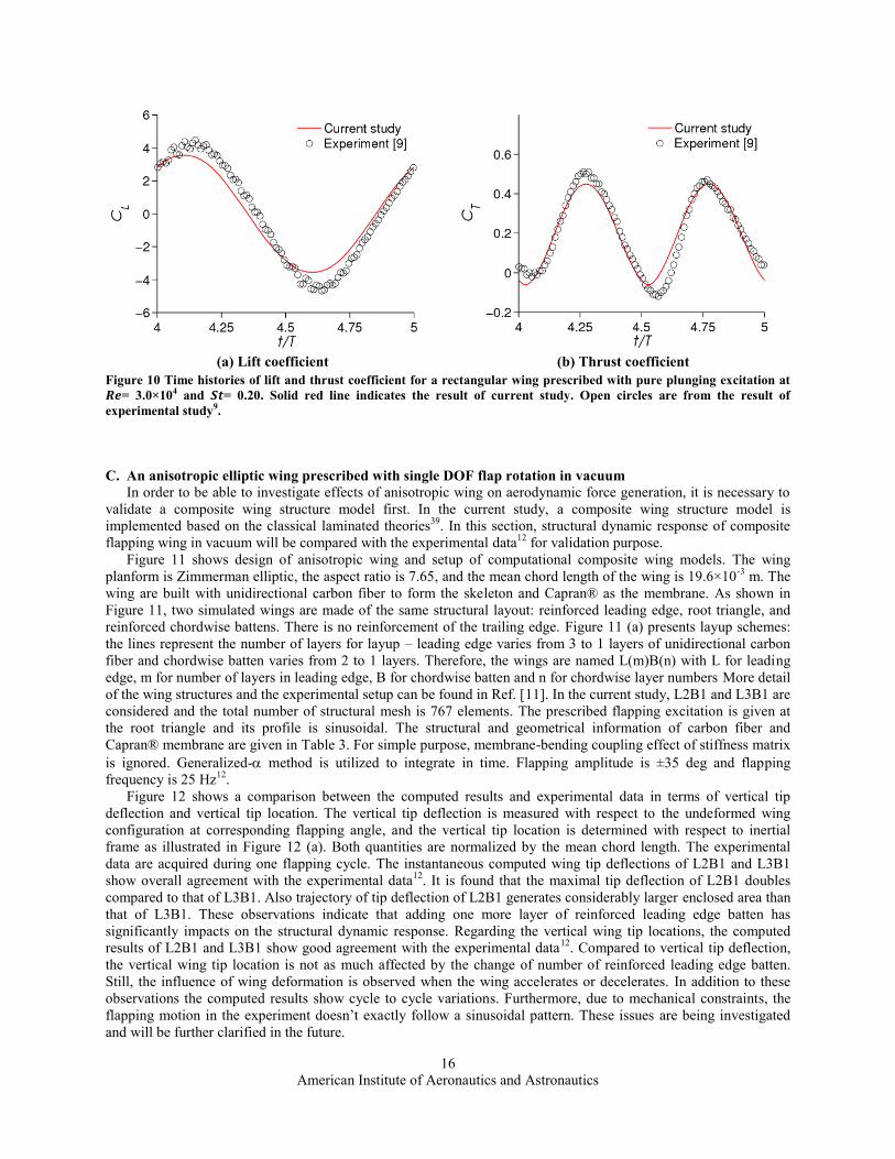
(a) Lift coefficient (b) Thrust coefficient
Figure 10 Time histories of lift and thrust coefficient for a rectangular wing prescribed with pure plunging excitation at
= 3.0×10⁴ and = 0.20. Solid red line indicates the result of current study. Open circles are from the result of
experimental study9.
C. An anisotropic elliptic wing prescribed with single DOF flap rotation in vacuum
In order to be able to investigate effects of anisotropic wing on aerodynamic force generation, it is necessary to
validate a composite wing structure model first. In the current study, a composite wing structure model is
implemented based on the classical laminated theories39
. In this section, structural dynamic response of composite
flapping wing in vacuum will be compared with the experimental data12
for validation purpose.
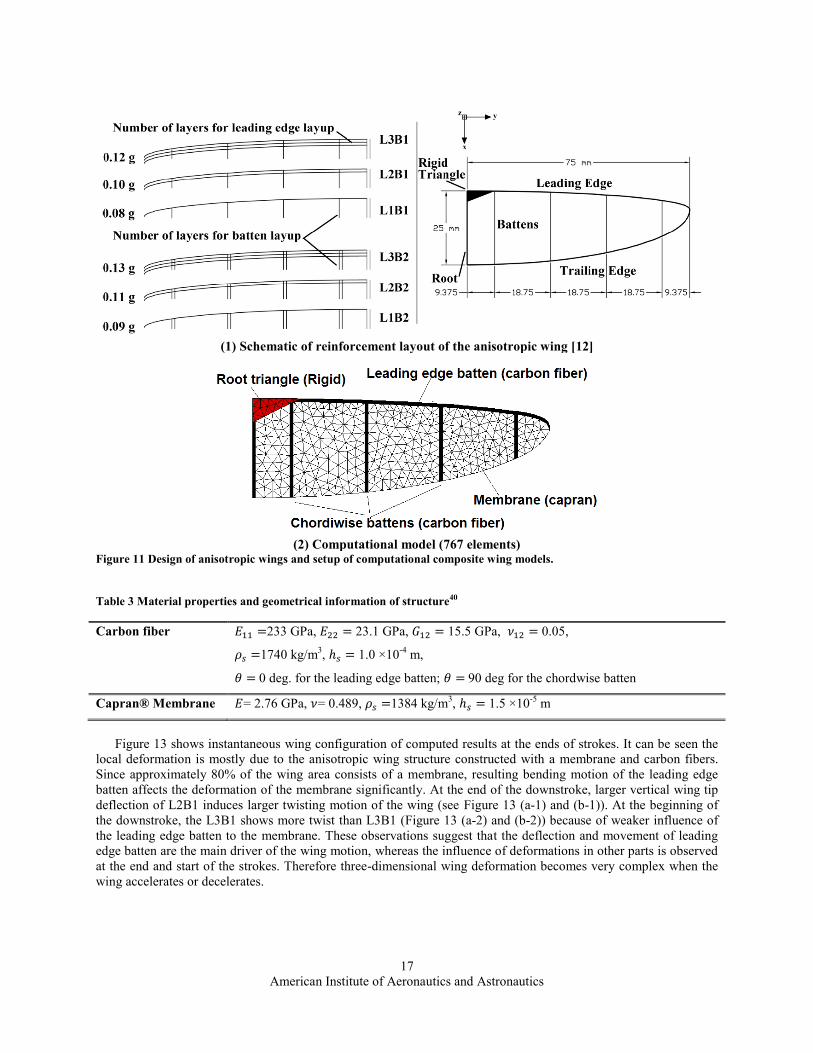
Figure 11 shows design of anisotropic wing and setup of computational composite wing models. The wing
planform is Zimmerman elliptic, the aspect ratio is 7.65, and the mean chord length of the wing is 19.6×10⁻³
m. The
wing are built with unidirectional carbon fiber to form the skeleton and Capran® as the membrane. As shown in
Figure 11, two simulated wings are made of the same structural layout: reinforced leading edge, root triangle, and
reinforced chordwise battens. There is no reinforcement of the trailing edge. Figure 11 (a) presents layup schemes:
the lines represent the number of layers for layup – leading edge varies from 3 to 1 layers of unidirectional carbon
fiber and chordwise batten varies from 2 to 1 layers. Therefore, the wings are named L(m)B(n) with L for leading
edge, m for number of layers in leading edge, B for chordwise batten and n for chordwise layer numbers More detail
of the wing structures and the experimental setup can be found in Ref. [11]. In the current study, L2B1 and L3B1 are
considered and the total number of structural mesh is 767 elements. The prescribed flapping excitation is given at
the root triangle and its profile is sinusoidal. The structural and geometrical information of carbon fiber and
Capran® membrane are given in Table 3. For simple purpose, membrane-bending coupling effect of stiffness matrix
is ignored. Generalized- method is utilized to integrate in time. Flapping amplitude is ±35 deg and flapping
frequency is 25 Hz12
.
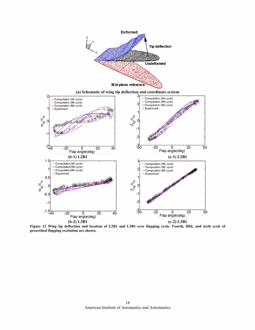
Figure 12 shows a comparison between the computed results and experimental data in terms of vertical tip
deflection and vertical tip location. The vertical tip deflection is measured with respect to the undeformed wing
configuration at corresponding flapping angle, and the vertical tip location is determined with respect to inertial
frame as illustrated in Figure 12 (a). Both quantities are normalized by the mean chord length. The experimental
data are acquired during one flapping cycle. The instantaneous computed wing tip deflections of L2B1 and L3B1
show overall agreement with the experimental data12
. It is found that the maximal tip deflection of L2B1 doubles
compared to that of L3B1. Also trajectory of tip deflection of L2B1 generates considerably larger enclosed area than
that of L3B1. These observations indicate that adding one more layer of reinforced leading edge batten has
significantly impacts on the structural dynamic response. Regarding the vertical wing tip locations, the computed
results of L2B1 and L3B1 show good agreement with the experimental data12
. Compared to vertical tip deflection,
the vertical wing tip location is not as much affected by the change of number of reinforced leading edge batten.
Still, the influence of wing deformation is observed when the wing accelerates or decelerates. In addition to these
observations the computed results show cycle to cycle variations. Furthermore, due to mechanical constraints, the
flapping motion in the experiment doesn’t exactly follow a sinusoidal pattern. These issues are being investigated
and will be further clarified in the future.
American Institute of Aeronautics and Astronautics
17
(1) Schematic of reinforcement layout of the anisotropic wing [12]
(2) Computational model (767 elements)
Figure 11 Design of anisotropic wings and setup of computational composite wing models.
Table 3 Material properties and geometrical information of structure40
Carbon fiber 233 GPa, 23.1 GPa, 15.5 GPa, 0.05,
1740 kg/m3, 1.0 ×10
-4 m,
0 deg. for the leading edge batten; 90 deg for the chordwise batten
Capran® Membrane = 2.76 GPa, = 0.489, 1384 kg/m3, 1.5 ×10
-5 m
Figure 13 shows instantaneous wing configuration of computed results at the ends of strokes. It can be seen the
local deformation is mostly due to the anisotropic wing structure constructed with a membrane and carbon fibers.
Since approximately 80% of the wing area consists of a membrane, resulting bending motion of the leading edge
batten affects the deformation of the membrane significantly. At the end of the downstroke, larger vertical wing tip
deflection of L2B1 induces larger twisting motion of the wing (see Figure 13 (a-1) and (b-1)). At the beginning of
the downstroke, the L3B1 shows more twist than L3B1 (Figure 13 (a-2) and (b-2)) because of weaker influence of
the leading edge batten to the membrane. These observations suggest that the deflection and movement of leading
edge batten are the main driver of the wing motion, whereas the influence of deformations in other parts is observed
at the end and start of the strokes. Therefore three-dimensional wing deformation becomes very complex when the
wing accelerates or decelerates.
American Institute of Aeronautics and Astronautics
18
(a) Schematic of wing tip deflection and coordinate system
(b-1) L2B1 (c-1) L2B1
(b-2) L3B1 (c-2) L3B1 Figure 12 Wing tip deflection and location of L2B1 and L3B1 over flapping cycle. Fourth, fifth, and sixth cycle of
prescribed flapping excitation are shown.

American Institute of Aeronautics and Astronautics
19
(a-1) L2B1 (Flap angle at tip = -35 deg) (b-1) L3B1 (Flap angle = -34.5 deg)
End-of-downstroke
(a-2) L2B1 (Flap angle at tip = 33.2 deg) (b-2) L3B1 (Flap angle = 35.66 deg)
End-of-upstroke
Figure 13 Wing deformation and vertical displacement of L2B1 and L3B1 in vacuum at end of strokes. Contour indicates
vertical displacement with respect to inertial frame.
D. A Zimmerman elliptic wing prescribed with pure flap rotation in hovering at Re= 1.5×10³ and k= 0.56
1. Rigid wing
A hovering rigid Zimmerman elliptic wing prescribed with pure flapping excitation = 1489 and = 0.56 is
simulated. The computational result is obtained using the parallel version NS solver with radial basis function
interpolation remeshing method. The Zimmerman planform, shown in Figure 14, flaps in a single degree of freedom
motion in still air.
A mixed structured and unstructured grid was used, which is the same as used in Ref. 18: the number of points in
the converged grid configuration is 0.5 million approximately. The computational setup is presented in Figure 15
and a summary of key parameters of this case are furnished in Table 4. The motion is excited at the rigid square at
the leading edge of the wing with a sinusoidal motion; see Eq. (8). For the boundary conditions for the outlet, the
pressure is set to zero. A no-slip condition on the flow velocity is assigned to the wing surface. The nodes on the
symmetry plane, the purple colored plane in Figure 15, are set to zero displacements. To assess the effect of
including the boundary nodes on the outer boundary surface in the remeshing system setup, in contrast to the results
presented in Section A, these boundary nodes are set to move freely in space and time. The radial basis function

American Institute of Aeronautics and Astronautics
20
support radius is 0.075, the half span length. By letting the outer boundary surfaces freely to move and taking
smaller support radius the computational efficiency is seen to be 20%.
Figure 14 Geometry of a Zimmerman planform.
(a) Overview of grid topology and size (b) wing grid
Figure 15 Computational setup for a flapping Zimmerman elliptic wing. (a) Overview of grid topology and
size; (b) Near the wing.
Table 4 Dimensional and dimensionless parameters for a Zimmerman elliptic wing prescribed with single DOF flap
rotation.
Parameter Value Dimensionless Parameter Value
Semi-span at quarter chord [m] 0.075 Chord-based Reynolds number 1489
Mean chord length [m] 0.0196 Reduced frequency 0.56
Flow velocity [m/s] 1.1 (mean tip speed) Aspect ratio 7.65
Air density [kg/m3] 1.23
Flapping amplitude [deg] 21
Flapping frequency [Hz] 10
Figure 16 shows time history of lift and drag coefficients for first three flapping cycle. It can be seen that the
drag coefficient is almost zero because of the wing kinematics considered in this study (i.e. symmetrical flapping
motion and no variation of angle of attack in time). Instantaneous lift peak is observed at early downstroke. Both
curve profiles of instantaneous lift and drag coefficient are comparable to the results of the stiffest wing case
presented in Ref. [18]. Figure 17 presents flow fields around the elliptic Zimmerman wing undergoing pure flapping
motion at the beginning and middle of downstroke. Three-dimensional vortical structures are visualized by iso-
vorticity magnitude and two-dimensional vortical structure is plotted by spanwise vorticity contours. Clearly, there
is three-dimensional vortical structure around the wing and an interaction between the flapping wing and vortex
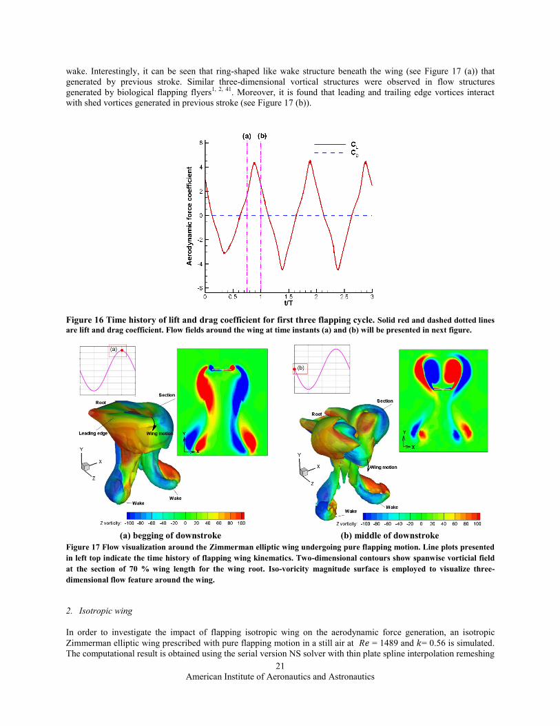
American Institute of Aeronautics and Astronautics
21
wake. Interestingly, it can be seen that ring-shaped like wake structure beneath the wing (see Figure 17 (a)) that
generated by previous stroke. Similar three-dimensional vortical structures were observed in flow structures
generated by biological flapping flyers1, 2, 41
. Moreover, it is found that leading and trailing edge vortices interact
with shed vortices generated in previous stroke (see Figure 17 (b)).
Figure 16 Time history of lift and drag coefficient for first three flapping cycle. Solid red and dashed dotted lines
are lift and drag coefficient. Flow fields around the wing at time instants (a) and (b) will be presented in next figure.
(a) begging of downstroke (b) middle of downstroke
Figure 17 Flow visualization around the Zimmerman elliptic wing undergoing pure flapping motion. Line plots presented
in left top indicate the time history of flapping wing kinematics. Two-dimensional contours show spanwise vorticial field
at the section of 70 % wing length for the wing root. Iso-voricity magnitude surface is employed to visualize three-
dimensional flow feature around the wing.
2. Isotropic wing
In order to investigate the impact of flapping isotropic wing on the aerodynamic force generation, an isotropic
Zimmerman elliptic wing prescribed with pure flapping motion in a still air at = 1489 and = 0.56 is simulated.
The computational result is obtained using the serial version NS solver with thin plate spline interpolation remeshing
American Institute of Aeronautics and Astronautics
22
method18
. The motion is excited at the rigid square at the leading edge of the wing with a sinusoidal motion; see Eq.
(8). In this study, two effective stiffnesses are considered: 1.4×10³ and 35.5×10
3. The density ratio and thickness
ratio of structure is 2.7 and 2.0×10⁻²
, respectively.
All structured grid around the Zimmerman wing of aspect ratio 7.65 is used and the number of points in the
converged grid configuration is 0.7 million approximately18
. The basic computational setup is similar to one
presented in Figure 11. For the outlet boundary condition, the pressure is set to zero. A no-slip condition on the flow
velocity is assigned to the wing surface. The nodes on the symmetry plane, the purple colored plane in, are set to
zero displacements.
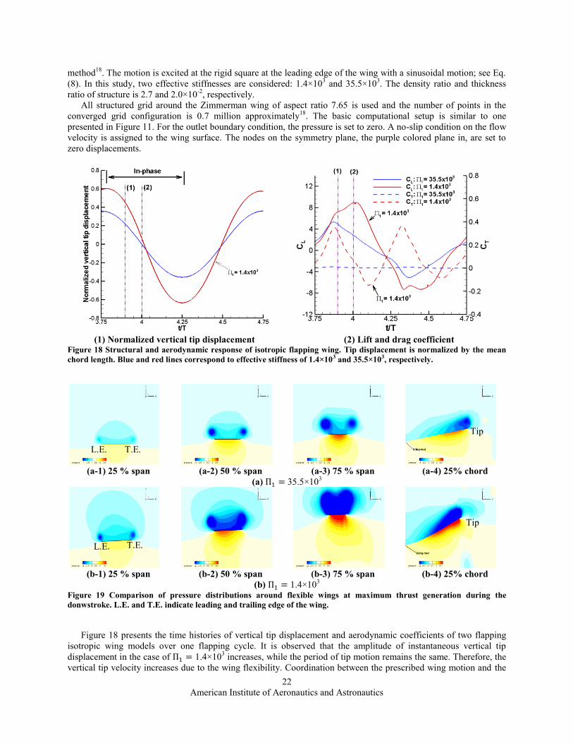
(1) Normalized vertical tip displacement (2) Lift and drag coefficient
Figure 18 Structural and aerodynamic response of isotropic flapping wing. Tip displacement is normalized by the mean
chord length. Blue and red lines correspond to effective stiffness of 1.4×10³ and 35.5×10³, respectively.
(a-1) 25 % span (a-2) 50 % span (a-3) 75 % span (a-4) 25% chord
(a) 35.5×10³
(b-1) 25 % span (b-2) 50 % span (b-3) 75 % span (b-4) 25% chord
(b) 1.4×10³
Figure 19 Comparison of pressure distributions around flexible wings at maximum thrust generation during the
donwstroke. L.E. and T.E. indicate leading and trailing edge of the wing.
Figure 18 presents the time histories of vertical tip displacement and aerodynamic coefficients of two flapping
isotropic wing models over one flapping cycle. It is observed that the amplitude of instantaneous vertical tip
displacement in the case of 1.4×10³ increases, while the period of tip motion remains the same. Therefore, the
vertical tip velocity increases due to the wing flexibility. Coordination between the prescribed wing motion and the
L.E. T.E.
L.E. T.E.
Tip
Tip
American Institute of Aeronautics and Astronautics
23
resultant tip movement shows in-phase motion during most of the stroke (see Figure 18 (a)). Previously Aono et al.4.
showed for plunging spanwise flexible wing that coordinated motion between the deformed wing and the rigidly
excited root is the underlying key mechanism for the flexibility enhanced aerodynamic force generation. Looking at
time histories of lift and drag coefficients, clearly, the case of 1.4×10³ produces thrust and larger lift than that
of 35.5×10³. (see Figure 18 (b)). This difference in the force generation is elicit in Figure 19 that shows the
pressure distributions at the three selected chordwise sections (25%, 50%, 75%) and one spanwise section (25%)
when the wing generates high thrust. It is found that for the case of 1.4×10³ flexibility induces positive
pitching angle (see Figure 19 (b-1, 2, 3)). This pitching angle changes the direction of resulting aerodynamic force
contributed by pressure favorable for the thrust generation. It should be mentioned that there is almost no camber of
the wing due to wing flexibility. This is consistent with the previous findings by Shyy et al.2 that the chordwise
flexibility elevates thrust generation by increased projected area of the deformed wing perpendicular to the
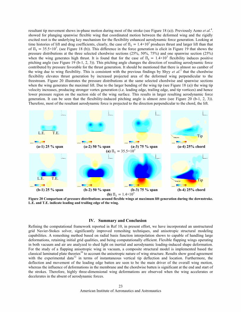
freestream. Figure 20 illustrates the pressure distributions at the same selected chordwise and spanwise sections
when the wing generates the maximal lift. Due to the larger bending of the wing tip (see Figure 18 (a)) the wing tip
velocity increases, producing stronger vortex generation (i.e. leading edge, trailing edge, and tip vortices) and hence
lower pressure region on the suction side of the wing surface. This results in larger resulting aerodynamic force
generation. It can be seen that the flexibility-induced pitching angle is almost zero (see Figure 20 (b-1, 2, 3)).
Therefore, most of the resultant aerodynamic force is projected to the direction perpendicular to the chord, the lift.
(a-1) 25 % span (a-2) 50 % span (a-3) 75 % span (a-4) 25% chord
(a) 35.5×10³
(b-1) 25 % span (b-2) 50 % span (b-3) 75 % span (b-4) 25% chord
(b) 1.4×10³
Figure 20 Comparison of pressure distributions around flexible wings at maximum lift generation during the downstroke.
L.E. and T.E. indicate leading and trailing edge of the wing.
IV. Summary and Conclusion
Refining the computational framework reported in Ref 10, in present effort, we have incorporated an unstructured
grid Navier-Stokes solver, significantly improved remeshing techniques, and anisotropic structural modeling
capabilities. A remeshing method based on radial basis function interpolation shows to capable of handling large
deformations, retaining initial grid qualities, and being computationally efficient. Flexible flapping wings operating
in both vacuum and air are analyzed to shed light on inertial and aerodynamic loading-induced shape deformation.
For the study of a flapping anisotropic wing in vacuum, a composite structural model is implemented based the
classical laminated plate theories39
to account the anisotropic nature of wing structure. Results show good agreement
with the experimental data12
in terms of instantaneous vertical tip deflection and location. Furthermore, the
deflection and movement of the leading edge batten are seen to be the main driver of the overall wing motion,
whereas the influence of deformations in the membrane and the chordwise batten is significant at the end and start of
the strokes. Therefore, highly three-dimensional wing deformations are observed when the wing accelerates or
decelerates in the absent of aerodynamic forces.
L.E. T.E.
L.E. T.E.
Tip
Tip
American Institute of Aeronautics and Astronautics
24
For the flapping Zimmerman rigid wing in still air at = 1.5×10³ and = 0.56 the aerodynamic force
generation is coupled with the vortex generation due to the wing motion. For the flapping isotropic Zimmerman
wing in still air, impacts of wing flexibility on the aerodynamic force generation is investigated. Two effective
stiffnesses are considered: 1.4×10³ and 35.5×10
3. The density ratio and thickness ratio of structure are 2.7 and
2.0×10⁻²
, respectively. In Refs 2 and 4, the implications of chordwise2 and spanwise
4 flexibility on aerodynamics
were investigated. Overall, the thrust generation consists of contributions due to both leading edge suction and the
pressure projection of the chordwise deformed rear foil. Even though the effective angle of attack and the net
aerodynamic force are reduced due to chordwise shape deformation, both mean and instantaneous thrust can be
enhanced due to the increase of projected area normal to the flight trajectory. For the spanwise flexible case,
correlations of the motion from the root to the tip play a role. Within a suitably selected range of spanwise
flexibility, the effective angle of attack and thrust forces of a plunging wing are enhanced due to the wing
deformations. These findings are in broad agreement with those observed in the present study: For an isotropic wing
two consistent mechanisms which can enhance thrust and lift are identified, namely
1) higher wing velocity due to larger bending motion can enhance the aerodynamic force,
2) flexibility-induced pitching angle can elevate thrust.
Acknowledgments
The work supported here has been supported in part by the Air Force Office of Scientific Research’s
Multidisciplinary University Research Initiative (MURI) grant and by the Michigan/AFRL (Air Force Research
Laboratory) Collaborative Center in Aeronautical Sciences. We thank Mr. Trizila and Dr. Wright for the fruitful
discussions provided.
References
1. Shyy, W., Lian, Y., Tang, J., Viieru, D., and Liu, H., Aerodynamics of low Reynolds number flyers New York:
Cambridge University Press, 2008.
2. Shyy, W., Aono, H., Chimakurthi, S.K., Trizila, P., Kang, C., Cesnik, C.E.S., and Liu, H., “Recent Progress in
Flapping Wing Aerodynamics and Aeroelasticity,” Progress in Aerospace Sciences, In Press, 2010,
doi:10.1016/j.paerosci.2010.01.001
3. Shyy, W., Lian, Y., Tang, J., Liu, H., Trizila, P., Stanford, B., Bernal, L., Cesnik, C.E.S., Friedmann, P., and Ifju,
P., “Computational Aerodynamics of Low Reynolds Number Plunging, Pitching and Flexible Wings For MAV
Applications,” Acta Mechanica Sinica, Vol. 24, pp.351-373, 2008.
4. Aono, H., Chimakurthi, S.K., Cesnik, C.E.S., Liu, H., and Shyy, W., “Computational Modeling of Spanwise
Effects on Flapping Wing Aerodynamics,” AIAA 2009-1270.
5. Ishihara, D., Yamashita, Y., Horie, T., Yoshida, S., and Niho, T., “Passive Maintenance of High Angle of Attack
and its Lift Generation during Flapping Translation in Crane Fly Wing,” Journal of Experimental Biology, Vol. 212,
pp. 3882-3891, 2009.
6. Gopalakrishnan, P., Tafti, D.K, “Effect of Wing Flexibility on Lift and Thrust Production in Flapping Flight,”
AIAA Journal, Vol. 48, No. 5, 2010.
7. Combes, S.A., Daniel, T.L., “Flexural Stiffness in Insect Wings I. Scaling and the Influence of Wing Venation,”
Journal of Experimental Biology, Vol. 206, pp. 2979-2987, 2003.
8. Combes, S.A., Daniel, T.L., “Flexural Stiffness in Insect Wings II. Spatial Distribution and Dynamic Wing
Bending,” Journal of Experimental Biology, Vol. 206, pp. 2989-2997, 2003.
9. Heathcote, S., Wang, Z., and Gursul, I., “Effect of Spanwise Flexibility on Flapping Wing Propulsion,” Journal
of Fluid & Structures, Vol. 24, pp. 183-199, 2008.
10. Chimakurthi, S.K., Tang, J., Palacios, R., Cesnik, C.E.S., Shyy W., “Computational Aeroelasticity Framework
for Analyzing Flapping Wing Micro Air Vehicles,” AIAA Journal, Vol. 47, Nr. 8, pp. 1865-1878, 2009.
11. Zhu, Q., “Numerical Simulation of a Flapping Foil with Chordwise or Spanwise Flexibility,” AIAA Journal, Vol.
45, No. 10, pp. 2448-2457, 2007.
12. Pin, W., Ifju P., Stanford, B., Sällström, E., Ukeiley, L., Love, R., and Lind, R., “A Multidisciplinary
Experimental Study of Flapping Wing Aeroelasticity in Thrust Production,” AIAA -2009-2413.
13. Anderson, J.D., Fundamentals of Aerodynamics, Second Edition, 1991, Singapore.
14. Ishihara, D., Yamashita, Y., Horie, T., Yoshida, S., and Niho, T., “A Two-dimensional Computational Study on
the Fluid-Structure Interaction Cause of Wing Pitch Changes in Dipteran Flapping Wing,” The Journal of
Experimental Biology, Vol. 212, pp. 3882-3891, 2009.
American Institute of Aeronautics and Astronautics
25
15. Lentink, D., and Dickinson, M.H., “Biofluiddynamic Scaling of Flapping, Spinning and Translating Fins and
Wings,” The Journal of Experimental Biology, Vol. 212, pp. 2691-2704, 2009.
16. Tang, J., Chimakurthi, S., Palacios, R., Cesnik, C.E.S., and Shyy, W., “Computational Fluid-Structure
Interaction of a Deformable Flapping Wing for Micro Air Vehicle Applications,” AIAA 2008-615.
17. Chimakurthi, S.K., Stanford, B.K., Cesnik, C.E.S., and Shyy, W., “Flapping Wing CFD/CSD Aeroelastic
Formulation Based on a Co-rotational Shell Finite Element,” AIAA 2009-2412.
18. Aono, H., Chimakurthi, S.K., Wu, P., Sällström, E., Stanford, B.K., Cesnik, C.E.S., Ifju, P., Ukeiley, L, and
Shyy, W., “A Computational and Experimental Study of Flexible Flapping Wing Aerodynamics,” AIAA 2010-554.
19. Gordnier, R.E., Attar P.J., Chimakurthi, S.K., and Cesnik, C.E.S., “Implicit LES Simulations of a Flexible
Flapping Wing,” AIAA 2010-2060.
20. McClung, A., Stanford, B., and Beran, P, “High-Fidelity Models for the Fluid-Structure Interaction of a Flexible
Heaving Airfoil,” AIAA 2010-2959.
21. Stanford, B., Kurdi, M., Beran, P., and McClung, A., “Shape-Structure, and Kinematic Parameterization of a
Power-Optimal Hovering Wing,” AIAA 2010-2963.
22. K. Stein, T. Tezduyar and R. Benney, “Mesh Moving Techniques for Fluid-Structure Interactions with Large
Displacements,” Journal of Applied Mechanics, Vol. 70, pp. 58-63, 2003.
23. Smith, R.W., and Wright, J.A., “A Classical Elasticity-Based Mesh Update Method for Moving and Deforming
Meshes,” AIAA 2010-164.
24. de Boer, A., van der Schoot, M.S., and Bijl, H., “Mesh Deformation Based on Radial Basis Function
Interpolation,” Computers and Structures, Vol. 85, pp. 784-795, 2007.
25. Rendall, T.C.S., and Allen, C.B., “Unified Fluid-Structure Interpolation and Mesh Motion using Radial Basis
Functions,” International Journal for Numerical Methods in Engineering, Vol. 74, pp. 1519-1559, 2008.
26. Rendall, T.C.S., and Allen, C.B., “Efficient Mesh Motion Using Radial Basis Functions with Data Reduction
Algorithms,” Journal of Computational Physics, Vol. 228, pp. 6231-6249, 2009.
27. Rendall, T.C.S., and Allen, C.B., “Reduced Surface Point Selection Options for Efficient Mesh Deformation
using Radial Basis Functions,” Journal of Computational Physics, Vol. 229, pp. 2810-2820, 2010.
28. Wright, J.A., and Smith, R.W., “An Edge-Based Method for the Incompressible Navier-Stokes Equations on
Polygonal Meshes,” Journal of Computational Physics, Vol. 169, pp. 24-43, 2001.
29. Kamakoti, R., and Shyy, W., “Evaluation of Geometric Conservation Law using Pressure-Based Fluid Solver
and Moving Grid Technique”, International Journal of Numerical Methods for Heat & Fluid Flow, Vol. 14, No. 7,
p. 851-865, 2006.
30. Luke, E.A., and George, T., “Loci: a rule-based framework for parallel multi-disciplinary simulation synthesis,”
Journal of Functional Programming, Vol. 15, Nr. 3, pp.477-502, 2005.
31. Shyy, W., “A Study of Finite Difference Approximations to Steady-State, Convection-Dominated Flow
Problems”, Journal of Computational Physics, Vol. 57, No. 3, 1985, pp. 415-438.
32. Shyy, W., Computational Modeling for Fluid Flow and Interfacial Transport, Elsevier, Amsterdam, 1994.
33. Blazek, J., Computational Fluid Dynamics: Principles and Applications, Elsevier, Amsterdam, 2001.
34. Thomas, P.D., and Lombard, K., “The Geometric Conservation Law – A Link between Finite-Difference and
Finite-Volume Methods of Flow Computation on Moving Grids”, AIAA paper 1978-1208, July 1978.
35. Balay, S., Buschelman, K., Gropp, W.D., Kaushik, D., Knepley, M.G., McInnes, L.C., Smith, B.F., and Zhang,
H, “PETSc Web page”, http://www.mcs.anl.gov/petsc, 2009.
36. Kamakoti, R., and Shyy, W., “Evaluation of Geometric Conservation Law using Pressure-Based Fluid Solver
and Moving Grid Technique”, International Journal of Numerical Methods for Heat & Fluid Flow, Vol. 14, No. 7,
p. 851-865.
37. Smith, R.W., and Wright, J.A., “An Implicit Edge-Based ALE Method for the Incompressible Navier-Stokes
Equations,” Int. J. Numer. Meth. Fluids, Vol 43, pp.253-279, 2003.
38. Beckert, A., and Wendland, H., “Multivariate Interpolation for Fluid-Structure-Interaction Problems using
Radial Basis Functions,” Aerospace Science and Technology, Vol. 5, Nr. 2, pp. 2-8, 2000.
39. Berthelot, J.-M., Composite Materials, Springer 1997.
40. Gogulapati, A., Friedmann, P. P., Khen, E., and Shyy W., “Approximate Aeroelastic Modeling of Flapping Wing
Comparison with CFD and Experimental Data,” AIAA 2010-2707.
41. Liu, H., and Aono, H., “Size effects on insect hovering aerodynamics: an integrated computational study,”
Bioinspiration and Biomimetics, Vol.4, No. 1, pp.1-13, 2009.