a practical assessment of the errors associated with full

A Practical Assessment of the Errors Associated with Full-Depth LADCP ProfilesObtained Using Teledyne RDI Workhorse Acoustic Doppler Current Profilers

A. M. THURNHERR

Lamont-Doherty Earth Observatory, Palisades, New York

(Manuscript received 9 April 2009, in final form 1 March 2010)

ABSTRACT

Lowered acoustic Doppler current profilers (LADCPs) are commonly used to measure full-depth velocity

profiles in the ocean. Because LADCPs are lowered on hydrographic wires, elaborate data processing is

required to remove the effects of instrument motion from the velocity measurements and to transform the

resulting relative velocity profiles into a nonmoving reference frame. Two fundamentally different methods

are used for this purpose: in the velocity inversion method, a set of linear equations is solved to separate the

ocean and instrument velocities while simultaneously applying a combination of velocity-referencing con-

straints from navigational data, shipboard ADCP measurements, and bottom tracking. In the shear method,

a gridded profile of velocity shear, which is not affected by instrument motion, is vertically integrated and

referenced using a single constraint. The main goals of the present study consist in estimating the accuracy of

LADCP-derived velocity profiles and determining which processing method performs better. To this purpose,

21 LADCP profiles collected during four surveys are compared to velocities measured simultaneously by

nearby moored instruments at depths between 2000 and 3000 m. The LADCP data were processed with two

slightly different publicly available implementations of the velocity inversion method, as well as with an im-

plementation of the shear method that was extended to support multiple simultaneous velocity-referencing

constraints. Regardless of the processing method, the overall rms LADCP velocity errors are ,3 cm s21 as

long as multiple velocity-referencing constraints are imposed simultaneously. On the other hand, solutions

referenced with a single constraint are associated with significantly greater errors. The two primary in-

strument characteristics that influence data quality are range and sampling rate. Dependence of the LADCP

velocity errors on those two parameters was determined by reprocessing range-limited subsets and temporal

subsamples of the LADCP data. Results indicate an approximately linear increase of the velocity errors with

decreasing sampling rate. The relationship between velocity errors and instrument range is much less linear

and characterized by a steep increase in velocity errors below a limiting range of ’60 m. To improve the

quality of the velocity data by increasing the instrument range, modern LADCP systems often include both

upward- and downward-looking ADCPs. The data analyzed here indicate that the addition of a second ADCP

can be as effective as doubling the range of a single-head LADCP system. However, in one of the datasets the

errors associated with the profiles calculated from combined up- and down-looker data are significantly larger

than the corresponding errors associated with the profiles calculated from the down-looker alone. The

analyses carried out here indicate that the velocity errors associated with LADCP profiles can be significantly

smaller than expected from previously published results and from the uncertainty estimates calculated by the

velocity inversion method.

1. Introduction

Eulerian measurements of ocean velocities are used in

many different contexts. Examples include transport esti-

mation of oceanic currents, as well as the study of physi-

cal oceanographic processes such as mesoscale eddies,

internal waves, etc. Acoustic Doppler current profilers

(ADCPs) are particularly useful for sampling the oceanic

velocity field because they yield velocity profiles, rather

than the point samples recorded by traditional current

meters. ADCPs obtain velocity profiles by transmitting

acoustic pulses (called pings) and measuring the Doppler

shift of sound energy reflected in the water column. The

velocities are sampled in fixed-size ‘‘depth cells’’ or ‘‘bins,’’

with the distance of a particular bin from the transducer

being determined by the time delay between a ping and its

echo return. The maximum distance from the transducer

where valid velocity measurements are obtained is called

Corresponding author address: A. M. Thurnherr, Lamont-Doherty

Earth Observatory, P.O. Box 1000, Palisades, NY 10964-1000.

E-mail: [email protected]

JULY 2010 T H U R N H E R R 1215

DOI: 10.1175/2010JTECHO708.1

� 2010 American Meteorological SocietyUnauthenticated | Downloaded 03/24/22 07:35 AM UTC

the ‘‘instrument range’’ and depends both on instrument

properties (transmit power and acoustic frequency) and on

the spatially and temporally varying acoustic scattering

properties of the ocean.

Most ADCPs are either permanently installed on ships,

where they sample the velocity field in the upper ocean

along the ship’s track, or deployed on moorings and bot-

tom mounts, where they collect Eulerian time series

measurements. Because of the limited range of ADCPs,

full-depth velocity profiles in the deep ocean cannot be

obtained with single instruments deployed in this manner.

This has led to the development of methods for process-

ing data from ADCPs that are lowered on hydrographic

wires, usually in conjunction with CTD systems. The pri-

mary instruments that are currently used for lowered

ADCP (LADCP) work are 3000-kHz broadband ADCPs

from the ‘‘Workhorse’’ product family manufactured by

Teledyne RD Instruments (RDI). In the open ocean be-

low the biologically productive surface layers, the typical

range of these instruments varies between a few 10s of

meters and ’200 m.

When used in LADCP systems, the ADCPs measure

velocity profiles relative to the moving instrument plat-

forms. To derive full-depth, absolute (i.e., in the earth’s

frame of reference) velocities from the short, relative

velocity profiles, the effects of the instrument motion

must be removed before the overlapping velocity pro-

files can be combined. There are two fundamentally

different methods that have been developed for pro-

cessing LADCP data:

1) Shear method: Because of the geometry of ADCP

measurements, translational instrument motions af-

fect the velocities in all bins equally, whereas rota-

tional motions around the center of the transducer

(pitch, roll, and heading changes) do not affect the

along-beam velocity measurements. Therefore, in-

strument motion does not affect vertical-shear pro-

files, which can be combined in overlapping averages

to span the full water depth. The horizontal velocity

profiles obtained by vertically integrating vertical-shear

data are relative to unknown integration constants,

which can be determined, for example, by tracking

the seabed near the bottom of a profile or from ship

drift estimated using navigational data (Firing and

Gordon 1990). The first successful application of the

LADCP shear method to derive full-depth absolute

velocity profiles is reported by Fischer and Visbeck

(1993), who find rms errors of ’5 cm s21 when

comparing a handful of deep LADCP casts in the

Tropical Atlantic to simultaneously obtained velocity

profiles obtained with acoustically tracked Pegasus

dropsondes.

2) Velocity inversion method: In its current imple-

mentations, the shear method does not allow multi-

ple velocity-referencing constraints (e.g., both from

navigational and bottom-tracking data) to be applied

simultaneously. Therefore, Visbeck (2002) developed

an alternative method for processing LADCP data

based on the fact that every ADCP velocity mea-

surement is the sum of ocean and instrument-package

velocities (as well as noise). For each LADCP cast

the velocity measurements define a system of linear

equations, with ocean and platform velocities as un-

knowns. Although the resulting equation systems are

singular, velocity-referencing constraints can easily be

added as additional equations. The most widely used

velocity-referencing constraints are derived from ship-

drift data, from bottom tracking, and from veloci-

ties measured by hull-mounted shipboard ADCPs.

The resulting overdetermined linear equation sys-

tems can be solved with standard inverse techniques

(e.g., Wunsch 1996) to yield estimates of ocean and

instrument-platform velocities.

Much of the early experience with LADCP systems

was gained during the second half of the World Ocean

Circulation Experiment (WOCE; King et al. 2001).

Processing of the WOCE LADCP data was carried out

primarily with an implementation of the shear method

developed by Eric Firing at the University of Hawaii.

This software uses navigational data, usually from a GPS

stream, to reference the relative velocity profiles, al-

though at least one group carried out experiments with

bottom tracking as an alternative (Cunningham et al.

1997). A particular shortcoming of LADCP velocities

derived with the shear method is the lack of information

about uncertainty, which has been estimated to be ‘‘a

few cm s21, except when backscattering is very low, or

something else goes wrong.’’ (King et al. 2001). In con-

trast, the velocity inversion method provides formal

uncertainty estimates (Visbeck 2002), which are, how-

ever, scaled semi-empirically—that is, it is not a priori

clear, how accurate they are. Interpretation of the for-

mal inversion uncertainty estimates is further compli-

cated because LADCP uncertainties are the combined

effects of different error sources with different vertical

correlation scales (Firing and Gordon 1990; King et al.

2001; Visbeck 2002).

The only fully satisfying method for assessing uncer-

tainties associated with LADCP-derived velocities con-

sists of comparing the data to independent measurements,

such as Pegasus profiles (e.g., Fischer and Visbeck

1993). Although shipboard ADCP (SADCP) velocities

can be used for the same purpose (e.g., Cunningham et al.

1997), this is not ideal because SADCP data also provide

1216 J O U R N A L O F A T M O S P H E R I C A N D O C E A N I C T E C H N O L O G Y VOLUME 27

Unauthenticated | Downloaded 03/24/22 07:35 AM UTC

useful velocity-referencing constraints for the LADCP

solutions. The purpose of the present study is to assess

the uncertainties associated with LADCP-derived veloc-

ities obtained with 300-kHz Teledyne RDI Workhorse

ADCPs. To this effect, LADCP data collected during

four surveys are compared to nearby velocity measure-

ments obtained with moored instruments (section 2a).

The data are processed using two different versions of

the velocity inversion method, with an implementation of

the shear method, as well as with a new inverse technique

that permits multiple simultaneous constraints to refer-

ence the relative velocities obtained with the shear method

(section 2b). Although rms errors of ’3 cm s21 can be

achieved when using all available velocity-referencing

constraints (section 3), the errors increase significantly

when subsets of the constraints are applied (section 4).

The performance of dual-head LADCP systems is usu-

ally, but not always, better than that of down-looker-only

systems (section 5). Effects of instrument range and sam-

pling rate are explored in section 6. Finally, it is shown that

velocity profiles derived from three-beam LADCP data

are associated with significantly increased velocity errors

(section 7). The main findings are discussed in section 8.

The appendix describes how the error estimates of the

current implementations of the velocity inversion method

are calculated.

2. Datasets and processing methods

a. Datasets

In August 2006, a CTD–LADCP survey was carried

out during the GRAVILUCK cruise to the crest of the

Mid-Atlantic Ridge near 378N 328W (Thurnherr et al.

2008). The LADCP system employed a single Teledyne

RDI Workhorse 300-kHz ADCP installed as a down-

looker on a CTD rosette. The ADCP was programmed

to record single-ping velocity ‘‘ensembles’’ in beam co-

ordinates. The bin length for the casts used here is 8 m,

the blanking distance was set to 0 m, and data from the

first bin are excluded from processing. To minimize the

effects of previous-ping interference from the seabed,

alternating ping intervals of 1 and 1.6 s were used (stag-

gered pinging; King et al. 2001). Four of the LADCP

profiles were taken less than 1 km from a bottom-

mounted ADCP (also a Teledyne RDI Workhorse) that

was deployed at a depth of 2080 m and recorded 10-ping

velocity ensembles once every minute.

In November 2006, another CTD–LADCP survey was

carried out during the LADDER-1 cruise to the crest of

the East Pacific Rise near 108N 1048W (Thurnherr et al.

2010, manuscript submitted to Deep-Sea Res.). Through-

out most of this survey, two Teledyne/RDI Workhorse

ADCPs were installed on a CTD rosette, although,

because of instrument failures, some casts were carried

out with a single ADCP installed as a down-looker.

The ADCP setup was identical to the one used during

the GRAVILUCK survey, except for slightly longer

pinging intervals of 1.5 and 2 s. During the LADDER-

1 cruise, five physical oceanography moorings with 15

Aanderaa RCM-11 acoustic current meters were de-

ployed. Additionally, a bottom-mounted ADCP (an-

other Teledyne RDI Workhorse) was deployed less

than 1 km from one of the moorings. Eight of the

LADCP profiles (five with a dual-head configuration)

were taken less than 1 km from one of the moored

instruments, all of which sampled the oceanic velocity

field every 20 min at depths between 2430 and 2930 m.

In December 2006–January 2007, a second CTD–

LADCP survey was carried out in the same region near

the East Pacific Rise during the LADDER-2 cruise

(Jackson et al. 2009). The LADCP system employed two

Teledyne RDI ADCPs installed on a CTD rosette. The

ADCPs were programmed the same way as during

LADDER-1. Five of the LADCP profiles were taken less

than 1 km from one of the moored instruments deployed

there in November 2006. A third CTD/LADCP survey

was carried out in the same region during the LADDER-3

cruise in November 2007 (Thurnherr et al. 2010, manu-

script submitted to Deep-Sea Res.). Again, two Teledyne

RDI ADCPs were installed on a CTD rosette and the

same instrument setup was used. Four of the LADCP

profiles from this survey were taken less than 1 km from

one of the moored instruments deployed there during

LADDER-1.

Combining the four datasets, there are 40 pairs of si-

multaneous nearby velocity samples from LADCP casts

and moored instruments. Because of the configuration

of the moorings, 34 of these velocity samples were ob-

tained within 150 m of the seabed, whereas the re-

maining ones were measured between 400 and 600 m

above the bottom (Fig. 1).

b. Data processing

Currently, there are three main publicly available

software packages used for LADCP data processing: 1)

an implementation of the shear method developed and

maintained by Eric Firing’s group at the School of

Ocean and Earth Science and Technology (SOEST) of

the University of Hawaii; 2) the original implementation

of the velocity inversion method developed by Martin

Visbeck and now maintained by this author at the

Lamont-Doherty Earth Observatory (LDEO); 3) a

cleaned up implementation of the velocity inversion

method maintained primarily by Gerd Krahmann at the

Leibniz Institute of Marine Sciences (IFM-GEOMAR,

or IFMG) in Kiel, Germany. For simplicity, the processing



packages will be referred to by the institutional abbrevi-

ations where they are maintained, that is, SOEST, LDEO

and IFMG. It should be noted that the IFMG and the

LDEO implementations are derived from (and share

much of) the same original code, that is, they are expected

to yield similar results.

The official versions of all three software packages

available in July 2008 are used for the present study, that

is, LDEO version IX_5 and IFMG version 10.6—the

SOEST software does not use version numbers. During

processing, several bugs in the LDEO software had to be

fixed to allow all possible combinations of the velocity-

referencing constraints to be used (section 4); the bug

fixes, which have been incorporated into version IX_6,

do not affect the default solutions derived using all three

constraints in any way. All three software packages have

‘‘free’’ parameters that can be modified by the user, al-

though there are many more in the LDEO and IFMG

velocity inversion implementations than in the SOEST

shear method software. Recommended values are used

throughout for all processing parameters. For the SOEST

and IFMG software packages, these are the default

values, but for the LDEO software the recommenda-

tions of the ‘‘how to’’ (Thurnherr 2009) were followed.

During the course of this investigation, it was found

that the profile quality is affected significantly by the

number of simultaneously applied velocity-referencing

constraints (section 4). To allow for a fair comparison

between the shear and the velocity inversion methods, a

new shear inversion method was implemented as follows.

For each velocity component of an LADCP profile a set

of linear equations is constructed relating the gridded

shear uz obtained with the SOEST software to the ve-

locities u, that is,

u(zi11)� u(zi)

zi11 � zi5 u

z

zi11 1 zi

2

� �. (1)

The velocities from the shipboard ADCP uSA and from

bottom tracking uBT define additional sets of equations

that reference the relative velocity profiles in the upper

ocean and near the seabed, respectively:

u(zi) 5 uSA

(zi) and (2)

u(zi) 5 uBT

(zi). (3)

Finally, the ship-drift (GPS) constraint is written as

a single equation

1

n�

iu(zi) 5 hui, (4)

where hui is the depth-averaged velocity taken from the

SOEST solution, and n is the number of velocity samples

in the profile. Expressions (1)–(4) define a set of linear

equations for the unknowns u(zi) that can be solved with

standard linear inverse techniques (e.g., Wunsch 1996).

For consistency, the bottom-tracking velocities are taken

from the solutions of the LDEO processing software,

although it is also possible to extract bottom-tracked

velocity profiles from LADCP data without running a full

velocity inversion.

3. Fully constrained down-looker solutions

For many applications, the most fundamental di-

agnostic of the quality of LADCP data is the accuracy

of individual (i.e., at a given depth) velocity estimates.

Here, this quantity is estimated from comparisons with

velocity measurements from nearby (,1 km horizontal

distance) current meters and bottom-mounted ADCPs.

Although bottom-mounted ADCPs measure velocity

profiles, the LADCP velocity errors at different depths

cannot be considered statistically independent. There-

fore, each bottom-mounted ADCP profile is vertically

averaged and the resulting velocity estimate is treated

the same way as a single current-meter sample. For

standard LADCP processing with any of the methods

described in section 2b, the down- and upcast data are

combined, which assumes that the ocean velocities do not

change significantly during a cast. Therefore, the velocity

measurements from the moored instruments are also

FIG. 1. Distribution of LADCP–mooring velocity pairs with height

above the seabed.



averaged over the durations of each LADCP cast. Figure 2

shows the LDEO-processed LADCP down-looker pro-

files associated with the smallest and largest discrepancies

with the simultaneously measured current-meter veloci-

ties. In both cases, the agreement between LADCP and

current-meter velocities is significantly better than that

indicated by the processing-derived errors—that is, the

uncertainties estimated by current implementations

of the velocity inversion method see the (appendix) are

overly conservative.

To obtain a statistical measure of the quality of

LADCP velocity samples, the individual velocity com-

ponents of the entire dataset are compared to the cor-

responding values from the moored instruments (Fig. 3).

These and all following comparisons are based on the

LADCP samples (at ’8 m vertical resolution) closest in

depth to the corresponding moored measurements, with-

out any extrapolation of the LADCP profiles below the

maximum depths. The overall rms discrepancies between

the LADCP and the moored-instrument velocity com-

ponents (2.6–3.4 cm s21) are significantly smaller than the

processing-derived velocity error estimates of 4–5 cm s21,

confirming that the latter are overly conservative. The

data furthermore indicate similar velocity discrepancies

for the samples from the bottom 150 m and for those

taken 400–600 m above the seabed (Figs. 3a–c). The

distributions of the velocity discrepancies are similar for

all three processing methods (Figs. 3d–f). The velocity

discrepancies associated with the different processing

methods are linearly correlated, although with rather

large rms misfits (’2.3 cm s21; not shown).

In addition to LADCP measurement and processing

errors, the rms discrepancies between the LADCP and

the moored-instrument velocities also include mea-

surement errors of the moored instruments, as well as

temporal and spatial oceanic variability. To quantify the

effects of these velocity uncertainties that are not caused

by LADCP errors, two of the moored-instrument re-

cords are used: between 9 November and 15 December

2006 a bottom-mounted ADCP deployed at a depth of

2570 m recorded velocity profiles every 20 min less than

200 m from a moored current meter recording velocities

at the same frequency and in the depth range of the

bottom-mounted ADCP measurements; averaging the

data over the typical duration of a CTD/LADCP cast

(2 h) yields rms velocity differences between the two

moored records of ’2 cm s21. Interpreting this value as

the uncertainty associated with an individual LADCP

velocity error estimate and assuming that the LADCP

velocity errors from different casts are statistically in-

dependent allows the uncertainties associated with rms

velocity discrepancies calculated from sets of LADCP

profiles to be estimated. For example, the rms velocity

discrepancies of the entire dataset (21 profiles) listed in

the caption of Fig. 3 are associated with uncertainties

of 0.4 cm s21 that are unrelated to LADCP measure-

ment and processing errors. This implies that the three

rms velocity discrepancies resulting from the different

FIG. 2. LADCP profiles from LDEO-processed down-looker data constrained with bottom-tracking, GPS, and

shipboard ADCP data, as well as simultaneous current-meter velocities. LADCP data are plotted with thin lines;

error bars show the processing-derived error estimates see the (appendix). Current-meter data are plotted with

thick error bars given by the standard errors estimated during time averaging and assuming independent sample

errors. (a) Profile with overall best agreement (0.8 cm s21 rms discrepancy) and (b) profile with overall worst

agreement (4.6 cm s21 rms discrepancy).



processing methods overlap within their uncertainties,

that is, the solutions are of similar quality. The discrep-

ancies between the LADCP velocities and the moored-

instrument measurements are significantly greater than

the uncertainties that are unrelated to LADCP mea-

surement and processing; therefore, in the following

they will simply be called LADCP velocity errors.

4. Velocity-referencing constraints

In the datasets analyzed here, the discrepancies be-

tween the fully constrained LADCP velocities and the

corresponding measurements from the moored instru-

ments are similar, regardless of the processing method

used (section 3). This observation is not particularly sur-

prising given the fact that 85% of the velocity measure-

ments from the moored instruments were made within

150 m of the seabed (Fig. 1), that is, in the depth range

where the package motion is directly constrained by

bottom tracking. Consistent with this consideration, the

LADCP velocity errors of the profiles constrained with

bottom tracking alone are similar to the corresponding

errors in the fully constrained solutions, and the LADCP

velocity errors from the different processing methods

constrained only by bottom tracking again agree within

their nominal uncertainty of 0.4 cm s21 (Table 1).

Whereas bottom tracking constrains the package mo-

tion near the seabed, shipboard ADCP data directly

constrain the LADCP velocities in the upper ocean (the

top 600–900 m in the datasets analyzed here). The con-

straint that has traditionally been most widely used in

LADCP processing, however, is based on ship drift in-

ferred from navigational (GPS) data (Fischer and Visbeck

1993). In contrast to bottom tracking and shipboard

ADCP measurements, both of which directly constrain

the LADCP velocities in particular depth ranges, ship

drift constrains the temporally and vertically averaged

ocean velocities. If the LADCP velocity errors are dom-

inated by uncorrelated single-ping errors of constant

magnitude, the LADCP velocity errors resulting from

using a constraint for the integrated velocities are small-

est in midwater and increase both toward the sea surface

and toward the seabed (Firing and Gordon 1990).

Consistent with these considerations, the rms LADCP

velocity errors in the datasets analyzed here increase

significantly for all processing methods when the ve-

locities are constrained by ship-drift (GPS) data alone

(Table 1). At first sight somewhat less expectedly, the

FIG. 3. Down-looker LADCP data vs current-meter velocities: (a)–(c) scatterplots of velocity components; (d)–(f) corresponding

histograms of velocity discrepancies; (a),(d) LDEO-processed solutions, 2.6 cm s21 rms velocity discrepancy; (b),(e) IFMG-processed

solutions, 3.4 cm s21 rms velocity discrepancy; and (c),(f) shear inverse solutions, 3.0 cm s21 rms velocity discrepancy.



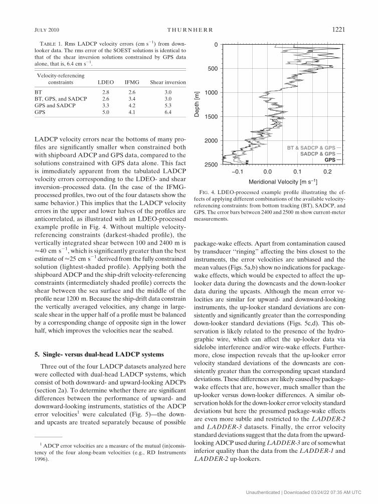
LADCP velocity errors near the bottoms of many pro-

files are significantly smaller when constrained both

with shipboard ADCP and GPS data, compared to the

solutions constrained with GPS data alone. This fact

is immediately apparent from the tabulated LADCP

velocity errors corresponding to the LDEO- and shear

inversion–processed data. (In the case of the IFMG-

processed profiles, two out of the four datasets show the

same behavior.) This implies that the LADCP velocity

errors in the upper and lower halves of the profiles are

anticorrelated, as illustrated with an LDEO-processed

example profile in Fig. 4. Without multiple velocity-

referencing constraints (darkest-shaded profile), the

vertically integrated shear between 100 and 2400 m is

’40 cm s21, which is significantly greater than the best

estimate of ’25 cm s21 derived from the fully constrained

solution (lightest-shaded profile). Applying both the

shipboard ADCP and the ship-drift velocity-referencing

constraints (intermediately shaded profile) corrects the

shear between the sea surface and the middle of the

profile near 1200 m. Because the ship-drift data constrain

the vertically averaged velocities, any change in large-

scale shear in the upper half of a profile must be balanced

by a corresponding change of opposite sign in the lower

half, which improves the velocities near the seabed.

5. Single- versus dual-head LADCP systems

Three out of the four LADCP datasets analyzed here

were collected with dual-head LADCP systems, which

consist of both downward- and upward-looking ADCPs

(section 2a). To determine whether there are significant

differences between the performance of upward- and

downward-looking instruments, statistics of the ADCP

error velocities1 were calculated (Fig. 5)—the down-

and upcasts are treated separately because of possible

package-wake effects. Apart from contamination caused

by transducer ‘‘ringing’’ affecting the bins closest to the

instruments, the error velocities are unbiased and the

mean values (Figs. 5a,b) show no indications for package-

wake effects, which would be expected to affect the up-

looker data during the downcasts and the down-looker

data during the upcasts. Although the mean error ve-

locities are similar for upward- and downward-looking

instruments, the up-looker standard deviations are con-

sistently and significantly greater than the corresponding

down-looker standard deviations (Figs. 5c,d). This ob-

servation is likely related to the presence of the hydro-

graphic wire, which can affect the up-looker data via

sidelobe interference and/or wire-wake effects. Further-

more, close inspection reveals that the up-looker error

velocity standard deviations of the downcasts are con-

sistently greater than the corresponding upcast standard

deviations. These differences are likely caused by package-

wake effects that are, however, much smaller than the

up-looker versus down-looker differences. A similar ob-

servation holds for the down-looker error velocity standard

deviations but here the presumed package-wake effects

are even more subtle and restricted to the LADDER-2

and LADDER-3 datasets. Finally, the error velocity

standard deviations suggest that the data from the upward-

looking ADCP used during LADDER-3 are of somewhat

inferior quality than the data from the LADDER-1 and

LADDER-2 up-lookers.

FIG. 4. LDEO-processed example profile illustrating the ef-

fects of applying different combinations of the available velocity-

referencing constraints: from bottom tracking (BT), SADCP, and

GPS. The error bars between 2400 and 2500 m show current-meter

measurements.

TABLE 1. Rms LADCP velocity errors (cm s21) from down-

looker data. The rms error of the SOEST solutions is identical to

that of the shear inversion solutions constrained by GPS data

alone, that is, 6.4 cm s21.

Velocity-referencing

constraints LDEO IFMG Shear inversion

BT 2.8 2.6 3.0

BT, GPS, and SADCP 2.6 3.4 3.0

GPS and SADCP 3.3 4.2 5.3

GPS 5.0 4.1 6.4

1 ADCP error velocities are a measure of the mutual (in)consis-

tency of the four along-beam velocities (e.g., RD Instruments

1996).



The accuracy of the processed velocity profiles is of

much greater importance than error velocity statistics,

of course. In the datasets analyzed here, the LDEO-

processed up-looker-only solutions are of similar quality

as the down-looker-only solutions, except in the case of

LADDER-3 (Table 2). The LADDER-1 and LADDER-2

velocity profiles calculated from combined up- and down-

looker data are associated with significantly smaller

LADCP velocity errors than either of the single-head

solutions, as expected from the increased effective range

of dual-head systems (Visbeck 2002). In the case of

LADDER-3, however, the addition of the up-looker data

decreases the quality significantly when compared to the

down-looker-only solutions. It is interesting to note that

the apparent problems with the LADDER-3 data are much

more severe for the solutions constrained with GPS data

alone. This observation indicates that the errors introduced

by combining the LADDER-3 up- and down-looker data

manifest themselves primarily as biased shear.

6. Effects of instrument range and sampling rate

Instrument range is an important factor affecting the

quality of LADCP data (Visbeck 2002), consistent with

the observation that the velocities derived from dual-

head LADCP systems can be associated with significantly

smaller LADCP velocity errors than those from down-

looker- or uplooker-only systems (section 5). Conversely,

in regions characterized by weak acoustic backscatter the

instrument range often becomes too small to calculate

full-depth LADCP velocity profiles (e.g., King et al.

2001). Within a given profile, the instrument range is not

a constant. In the case of the LADDER data, all instru-

ments are associated with ranges exceeding 20 bins in

the upper ocean and approximately constant minimum

ranges of 10–12 bins below 1500 m or so. To quantify

the relationship between instrument range and LADCP

profile quality, the dual-head profiles from LADDER-1

and LADDER-2 were reprocessed several times by the

FIG. 5. Error velocities of the datasets collected with dual-head LADCP systems: (a),(b) cruise-averaged mean

values; (c),(d) standard deviations; (a),(c) downcasts; and (b),(d) upcasts.



LDEO software with artificially limited instrument

ranges obtained by discarding data from the farthest bins

(Fig. 6). The GRAVILUCK data are not used for this

comparison because they were collected with a down-

looker-only system and in a region characterized by a

different scattering environment; and the LADDER-3

profiles are not used because of the inconsistencies be-

tween the down- and up-looker data (section 5). Con-

sistent with expectations, the LADCP velocity errors

decrease with increasing instrument range up to the deep-

water range determined by the scattering environment.

In the data analyzed here, a minimum of seven 8-m bins

are required to derive LADCP velocity profiles with er-

rors ,5 cm s21; restricting the instrument range to less

than five bins results in numerous profiles that cannot be

processed any more.

Inspection of Fig. 6 indicates close agreement between

the dual-head and down-looker LADCP velocity errors

for instrument ranges between eight bins (four from each

instrument in the case of the dual-head LADCP) and the

maximum effective instrument range of single-head sys-

tems (’10 bins). At shorter instrument ranges, the dual-

head LADCP velocity errors are larger, most likely

because the first bin is always discarded (section 2a)—that

is, at an instrument range of six bins, a dual-head single-

ping profile consists of four velocities (bins 2 and 3 from

each instrument), whereas the corresponding single-head

single-ping profile consists of five velocities (bins 2–6).

The agreement for instrument ranges of 8–10 bins implies

that adding an upward-looking ADCP can be as good as

doubling the range of a down-looker-only system.

In addition to increasing the effective instrument

range by adding a second ADCP, increasing the sam-

pling rate is also expected to improve the LADCP data

quality (Firing and Gordon 1990). To elucidate the ef-

fects of the pinging rate on the LADCP velocity errors,

the down-looker data from the three LADDER cruises

were reprocessed by the LDEO software with different

subsets of the recorded single-ping ensembles. The

GRAVILUCK data are not used for this comparison be-

cause of the different sampling rate. Because staggered

pinging was used to avoid data gaps caused by the previous-

ping interference (section 2a), consecutive pairs of single-

ping profiles were kept in the subsets used for processing;

for example, the profiles with a mean sampling rate of

5.25 s were calculated by discarding single-ping profiles

1–4, keeping 5 and 6, discarding 7–10, etc. Within the

explored range of sampling rates, the LADCP velocity

errors increase approximately linearly with increasing

sampling intervals (Fig. 7).

7. Three-beam solutions

Single-beam failures are a fairly common hardware

problem of LADCP systems. In principle, such single-

beam failures are not catastrophic because three beams

are sufficient for determining the three components of

the oceanic velocity field. To assess the degradation in

data quality associated with three-beam solutions, the

down-looker LADCP data were reprocessed 14 times

with the LDEO software and constrained with shipboard

ADCP and GPS data after discarding the velocities from

a randomly chosen beam (a different one for each profile)

of each instrument. Comparison with the solutions de-

rived from all four beams indicates that the LADCP ve-

locity errors associated with the three-beam solutions

tend to be larger than the LADCP velocity errors asso-

ciated with the four-beam solutions, except in the case of

GRAVILUCK where the three- and four-beam solutions

are of similar quality (Table 3). Except in the case of

LADDER-3, there are three-beam solutions associated

with smaller LADCP velocity errors than those of the

four-beam solutions, however. Averaged over the four

datasets, the mean three-beam LADCP velocity error is

4.2 6 0.4 cm s21, which is significantly greater than the

3.3 cm s21 associated with the the four-beam solutions.

The reduction in data quality is therefore similar to the

effect of halving the sampling frequency (Fig. 7).

Occasionally, LADCP data show evidence for con-

tamination by instrument package wakes. Although no

evidence for significant wake contamination was found in

the data analyzed here (section 5), the profiles were nev-

ertheless reprocessed with the LDEO software after dis-

carding from each ensemble the velocities from the beam

pointing in the instantaneous downstream direction. For

all datasets considered here, the corresponding LADCP

velocity errors lie within the range of the ‘‘3 random

beams’’ solutions (Table 3), consistent with the prior

TABLE 2. LDEO-processed LADCP velocity errors (cm s21) from surveys carried out with dual-head instruments. The LADDER-1 data

include three profiles collected with a down-looker-only system (section 2a).

Dataset Number profiles

GPS- and SADCP- constrained GPS-constrained

Down-looker Up-looker Dual head Dual head

LADDER-1 8 3.2 3.1 2.5 4.3

LADDER-2 5 3.6 3.7 2.4 3.6

LADDER-3 8 2.8 5.0 4.4 10.4



inference that package-wake contamination does not

affect these velocity profiles significantly.

8. Discussion

a. Representativeness of the datasets analyzed here

The main purpose of the present study is to provide

quantitative estimates of the uncertainties associated

with LADCP-derived velocity profiles. The data ana-

lyzed here indicate that, in regions of sufficient scatter-

ing, LADCPs can be used to measure instantaneous

velocities with rms uncertainties between 2 and 3 cm s21,

although the LADCP velocity error distributions shown

in Fig. 3 indicate that outliers associated with signifi-

cantly larger errors are common. For a given profile, the

smallest LADCP velocity errors are expected in the

depth ranges where the velocity-referencing constraints

directly affect the solutions, that is, near the seabed for

bottom tracking, near the sea surface for shipboard ADCP

data, and at mid-depth for the ship-drift (GPS) constraint.

Consistent with this expectation, the LADCP velocity

errors estimated here increase from 3.0 6 0.4 cm s21

when all constraints are used to 4.3 6 1.0 cm s21 without

bottom tracking (Table 1). When only the ship-drift

constraint is used, the LADCP velocity errors increase

further to 5.2 6 1.2 cm s21, which is similar to pre-

viously reported errors for GPS-only constrained pro-

files collected with different instruments in other regions

(e.g., Fischer and Visbeck 1993; Cunningham et al. 1997).

Therefore, the results derived here are considered rep-

resentative for the LADCP data collected, for example,

during the WOCE and Climate Variability and Predict-

ability (CLIVAR) projects.

A potentially significant limitation of the datasets

analyzed here is the fact that 85% of the moored velocity

samples were recorded in the bottom 150 m of the water

column, where the LADCP velocities are directly con-

strained by bottom tracking. It is reiterated, however,

that the LADCP velocity errors associated with the re-

maining 15% of the samples, which were recorded 400–

600 m above the seabed, are not significantly greater than

the errors associated with the near-bottom samples

(Fig. 3). Nevertheless, all tests of the effects of dual-

headed systems (section 5), instrument range and sam-

pling rate (section 6), and three-beam solutions (section 7)

were carried out without using bottom-track data. The

resulting velocities near the seabed are, therefore, ver-

tically separated by more than 1000 m from the closest

‘‘velocity-referencing level’’ at middepth for the GPS

constraint. This is similar to the maximum vertical dis-

tance of any LADCP velocity from the nearest velocity-

referencing level for a 5000-m cast constrained by bottom

tracking, shipboard ADCP data, and GPS measure-

ments, again suggesting that the results derived here

can be considered representative for full-depth LADCP

profiles.

Acoustic backscatter is the most important environ-

mental parameter affecting ADCP range and, therefore,

the quality of the LADCP velocities. To put the scatter-

ing environment of the data analyzed here into a wider

context, the minimum deep-water instrument ranges were

FIG. 6. LADCP velocity errors vs instrument range for the LDEO-

processed dual-head profiles from LADDER-1 and LADDER-2.FIG. 7. LADCP velocity errors vs sampling rate for the LADDER

down-looker datasets, processed with the LDEO software and

constrained with GPS and shipboard ADCP data.



determined for all stations of a recent meridional sec-

tion across the eastern Pacific between 208N and 708S

(CLIVAR P18), where LADCP data were collected with

a dual-head Workhorse-based system and an identical

instrument setup to the one used here (Fig. 8). Although

the instrument range of the LADCP data analyzed here

(10–12 8 m bins in the deep water below 1500 m; Section 6)

is somewhat above the average observed during CLIVAR

P18, Fig. 6 implies that the expected LADCP velocity

errors of most of the P18 profiles are nevertheless

,4 cm s21.

b. Obtaining high-quality LADCP velocity profiles

In general, the errors associated with LADCP-derived

velocities are caused by a combination of unbiased ran-

dom measurement errors, shear bias, as well as velocity-

referencing uncertainties. Previous analyses of LADCP

velocity errors deal primarily with unbiased random er-

rors (Firing and Gordon 1990; Visbeck 2002), although

King et al. (2001) also discuss strong shear bias errors that

contaminate a (small) subset of LADCP profiles to the

point where the down- and upcast profiles are clearly

inconsistent. It should be noted, however, that shear bias

errors are difficult to distinguish from unbiased random

errors—Firing and Gordon (1990) show that the veloc-

ity errors associated with vertically integrated LADCP-

derived shear increase with increasing vertical wavelength

even in the absence of shear bias, that is, the expected

vertically averaged shear error does not vanish. Fortu-

nately, applying multiple simultaneous velocity-referencing

constraints reduces not just shear bias errors but also the

LADCP velocity errors associated with unbiased random

velocity errors (section 4).

In addition to applying multiple simultaneous velocity-

referencing constraints to reduce the shear errors on

large vertical scales, the primary method for improving

the accuracy of LADCP velocities consists of increasing

sampling by extending the instrument range and/or in-

creasing the pinging rate. For a given ADCP the maxi-

mum achievable sampling rate is limited by the number

of bins to be stored and the time required for data pro-

cessing and storage. Besides lowering the acoustic fre-

quency, which requires transducer modifications, the

instrument range can potentially be extended by in-

creasing the acoustic power transmitted into the water

column. Recent tests carried out with a ‘‘high-power’’

300-kHz Workhorse prototype instrument have not yiel-

ded noticeable improvements in data quality, however

(Liang and Thurnherr 2009). Given the lack of cur-

rently available ADCPs with acoustic frequencies be-

low 300 kHz and suitable for LADCP work, the only

remaining option for increasing the instrument range

consists of using dual-head LADCP systems. The results

from LADDER-1 and LADDER-2 indicate that the data

quality obtainable with dual-head systems can be as good

as doubling the range of a single instrument. Besides in-

creasing the instrument range, dual-head LADCP sys-

tems have the added advantage that they avoid data gaps

caused by sidelobe interference from the seabed, which

affects the ship-drift velocity constraint (King et al. 2001).

The reduced internal consistency of uplooker data ap-

parent in error-velocity statistics (Fig. 5) is most likely

related to the presence of the hydrographic wire on which

TABLE 3. LDEO-processed down-looker LADCP velocity errors (cm s21) for four- and three-beam solutions, constrained by GPS and

shipboard ADCP data. The mean values and ranges (in parentheses) of the ‘‘three random beams’’ solutions are estimated from 14

reprocessing runs.

Dataset No. of profiles All beams Three random beams Three upstream beams

LADDER-1 8 3.2 3.6 (2.6–5.0) 3.8

LADDER-2 5 3.6 4.2 (3.2–5.2) 3.9

LADDER-3 8 2.8 4.8 (3.9–5.9) 5.8

GRAVILUCK 4 4.2 4.2 (3.3–5.5) 4.2

FIG. 8. Single-instrument deep-water range observed during

CLIVAR P18 cruise.



the LADCP system is suspended—both sidelobe inter-

ference and wakes are possible. However, these wire ef-

fects apparently have no significant effect on the quality

of the processed velocity profiles.

In contrast to LADDER-1 and LADDER-2, the

LADCP velocity errors for LADDER-3 are smallest

when the down-looker data are processed alone, im-

plying up- versus down-looker data inconsistencies. A

likely cause of these inconsistencies are pitch, roll, and/

or heading measurement errors, which occur in all dual-

head LADCP datasets, not just in those analyzed here.

However, the quality of the LADDER-3 dual-head so-

lutions does not change significantly when the data are

reprocessed after disabling the code (identical in the

LDEO and IFMG software) that is intended to correct

for pitch and roll inconsistencies or when the data are

reprocessed without using measurements from either

one of the two compasses (not shown). A bad beam

is another possible cause for the apparent up- versus

down-looker data inconsistencies. The LADDER-3 up-

looker is particularly suspect in this respect because the

corresponding single-head solutions are associated with

the largest LADCP velocity errors of any single-head

profiles derived here (Table 2). However, none of the

solutions from eight additional LADDER-3 reprocessing

runs with the LDEO software, each carried out without

data from a particular beam, is associated with smaller

LADCP velocity errors than the LADDER-3 down-

looker-only profiles (not shown). This observation indi-

cates that the up- versus down-looker data inconsistencies

are not caused by a (single) bad beam. Although it has

not been possible to determine the exact nature of the

problem(s) affecting the LADDER-3 data, it was found

that the bin-averaged inversion residuals (those compo-

nents of the noise vector n in expression (A1) of the ap-

pendix corresponding to the LADCP velocities) of

the bins closest to the ADCPs are significantly biased,

whereas no such biases are found in the LADDER-1 and

LADDER-2 data (Fig. 9). A corresponding diagnostic

figure was therefore added to the output of the LDEO

software version IX_6.

For the present study three different publicly available

software packages were used to process the LADCP

data. Two are based on the velocity inversion method of

Visbeck (2002), and the remaining one is an extension of

the SOEST implementation of the shear method, which

was used extensively during WOCE. No consistent quality

difference between the different processing methods was

found. Although high-quality LADCP profiles can be

obtained with either of the processing systems used here,

it is clear that multiple velocity-referencing constraints

significantly increase the quality of the solutions. There-

fore, the quality of the WOCE-era LADCP data processed

with the SOEST software could be improved significantly

by reprocessing with an inversion-based method. Pro-

cessing LADCP data with multiple methods can be

valuable for detecting problem profiles (e.g., Thurnherr

et al. 2008), which is particularly important in regions

of marginally sufficient scattering. Therefore, continued

maintenance of at least one implementation of both

processing methods is advisable.

Acknowledgments. I learned most of what I know

about LADCPs from numerous discussions with Eric

FIG. 9. Mean inversion residuals of the meridional velocity components from two dual-head example casts: (a)

example cast from LADDER-1 and (b) example cast from LADDER-3, where inconsistencies between the data

from the two ADCPs cause biased residuals in the bins closest to the instruments.



Firing and Martin Visbeck, who pioneered the use of

this instrument system. Without their publicly available

processing packages, and the additional user support

provided by Jules Hummon and Gerd Krahmann, this

study would not have been possible. Both Eric and

Martin contributed valuable comments on an early draft

of this manuscript and additional comments by two

anonymous reviewers are gratefully acknowledged.

During my first LADCP cruise, John Church motivated

me to develop an early version of the shear inversion

method. The LADDER data were collected under the

U.S. National Science Foundation Grant 0425361. The

LADDER-2 data were acquired and processed by Jim

Ledwell and Ryan Jackson. The GRAVILUCK survey

was funded by the U.S. National Science Foundation

under Grant 0550730, with additional support from the

French IDAO/LEFE GRAVILUCK project. Phil Mele

carried out all processing with the IFMG software.

APPENDIX

Velocity Inversion Error Estimates

The velocity inversion method of Visbeck (2002) con-

sists of solving the system of linear equations

d 5 Gm 1 n, (A1)

where G is the ‘‘model matrix’’ that relates the velocity

measurements (vector d, which contains LADCP, SADCP,

bottom-tracking, and ship-drift velocities) to the CTD-

package and ocean velocities (vector m). The ‘‘noise’’

vector n represents measurement errors and errors

caused by imperfect predictions of the measured ve-

locity field by Gm (data and model errors). The formal

velocity errors estimated by both the LDEO and IFMG

implementations of the velocity inversion method are

derived from the diagonal elements of the model pa-

rameter covariance matrix C given by expression (37) of

Visbeck (2002); that is

C 5 s2d(GTG)�1, (A2)

where sd is a measure of the data uncertainty, which is

assumed to be constant. As implemented, a velocity

error profile is first calculated using

e1(z) 5

ffiffiffiffiffiffiffiffiffiffiffiffiffiffiffiffiffiffiffiffidiag

oc(C)

pmedian[

ffiffiffiffiffiffiffiffiffiffiffiffiffiffiffiffiffiffiffiffidiag

oc(C)

p]

3 median[s(z)], (A3)

where diagoc(C) denotes the diagonal elements of the

covariance matrix C that correspond to the ocean ve-

locity estimates, and s(z) is the profile of the standard

deviations of all ocean velocity estimates at each depth.

[At each depth, there are generally multiple ocean ve-

locity samples from multiple partially overlapping (su-

per)ensembles.] At the end of each velocity inversion,

the baroclinic velocities are additionally estimated using

an implementation of the shear method. If the standard

deviation of the differences between the two baroclinic

velocity profiles s is larger than the mean inversion-derived

velocity error estimate he1(z)i, the velocity error profile is

then empirically rescaled using

e2(z) 5

e1(z)

he1(z)i 3

s

1.5. (A4)

REFERENCES

Cunningham, S. A., M. J. Griffiths, and B. A. King, 1997: Com-

parison of bottom-tracking and profiling LADCP data in

a section across the ACC at Drake Passage. International

WOCE Newsletter, No. 26, WOCE International Project Of-

fice, Southampton, United Kingdom, 39–40.

Firing, E., and R. Gordon, 1990: Deep ocean acoustic Doppler

current profiling. Proc. IEEE Fourth Working Conf. on Cur-

rent Measurements, Clinton, MD, Institute of Electrical and

Electronics Engineers, 192–201.

Fischer, J., and M. Visbeck, 1993: Deep velocity profiling with

self-contained ADCPs. J. Atmos. Oceanic. Technol., 10, 764–

773.

Jackson, P. R., J. R. Ledwell, and A. M. Thurnherr, 2009: Dis-

persion of a tracer on the East Pacific Rise (98N to 108N), in-

cluding the influence of hydrothermal plumes. Deep-Sea Res. I,

57, 37–52.

King, B. A., E. Firing, and T. M. Joyce, 2001: Shipboard observa-

tions during WOCE. Ocean Circulation & Climate, G. Siedler

et al., Eds., Academic Press, 99–122.

Liang, X., and A. M. Thurnherr, cited 2009: Evaluating a high-

power prototype of the Teledyne/RDI Workhorse ADCP.

[Available online ftp://ftp.ldeo.columbia.edu/pub/LADCP/

Reports/HP_Workhorse.pdf.]

RD Instruments, 1996: Acoustic Doppler Current Profiler: Prin-

ciples of operation; a practical primer. RD Instruments, 52 pp.

Thurnherr, A. M., cited 2009: How to process LADCP data with

the LDEO software. [Available online at ftp://ftp.ldeo.columbia.

edu/pub/LADCP/HOWTO.]

——, G. Reverdin, P. Bouruet-Aubertot, L. St. Laurent,

A. Vangriesheim, and V. Ballu, 2008: Hydrography and flow in

the Lucky Strike segment of the Mid-Atlantic Ridge. J. Mar.

Res., 66, 347–372.

Visbeck, M., 2002: Deep velocity profiling using lowered acoustic

Doppler current profilers: Bottom track and inverse solutions.

J. Atmos. Oceanic. Technol., 19, 794–807.

Wunsch, C., 1996: The Ocean Circulation Inverse Problem. Cam-

bridge University Press, 442 pp.



CORRIGENDUM

A. M. THURNHERR

Lamont-Doherty Earth Observatory, Palisades, New York

(Manuscript received and in final form 14 March 2011)

The Acknowledgments section in Thurnherr (2010) contains erroneous information

regarding the GRAVILUCK LADCP survey. The GRAVILUCK LADCP survey was

carried out in the context of the French GRAVILUCK project, which provided ship

time, instrumentation, as well as personnel support. The oceanographic component of

GRAVILUCK was funded in the context of the IDAO/LEFE research program. Funding for

the author’s participation on the cruise and for analysis of the GRAVILUCK LADCP data

was provided by the U.S. National Science Foundation under Grant 0550730.

REFERENCE

Thurnherr, A. M., 2010: A practical assessment of the errors associated with full-depth LADCP profiles

obtained using Teledyne RDI Workhorse acoustic Doppler current profilers. J. Atmos. Oceanic Technol.,

27, 1215–1227.

Corresponding author address: A. M. Thurnherr, Lamont-Doherty Earth Observatory, P.O. Box 1000, Palisades, NY 10964-1000.

E-mail: [email protected]


DOI: 10.1175/JTECHD-11-00042.1

� 2011 American Meteorological SocietyUnauthenticated | Downloaded 03/24/22 07:35 AM UTC

a practical assessment of the errors associated with full

Documents