A report by JGS chapter of TC23 limit state design ingeotechnical engineering practice

Geotechnical Risk and Safety – Honjo et al. (eds)© 2009 Taylor & Francis Group, London, ISBN 978-0-415-49874-6

Code calibration in reliability based design level I verificationformat for geotechnical structures

Y. Honjo, T.C. Kieu Le & T. HaraGifu University, Gifu, Japan

M. ShiratoPublic Works Research Institute, Tsukuba, Japan

M. SuzukiResearch Institute, Shimizu Corporation, Tokyo, Japan

Y. KikuchiPort and Airport Technical Research Institute, Yokosuka, Japan

ABSTRACT: This report is prepared by a working group in JGS chapter of TC23 Limit State Design inGeotechnical Engineering Practice and summarizes the important points to note and recommendations whennew design verification formulas are developed based on Level I reliability based design (RBD) format.

There are several different types of verification format in RBD Level I such as partial factor method (PFM), loadand resistance factor design (LRFD), etc. LRFD format is recommended in this report as the most suitable veri-fication format at present based on the following reasons: (1) a designer can trace the most likely behavior of thestructure to the very last stage of design if the characteristic values of the resistance basic variables are appropri-ately chosen, (2) the format can accommodate a performance function with high non-linearity and with some basicvariables to both force and resistance side, and (3) code calibration is possible for the case only total uncertaintyof the design method is known and the total uncertainty cannot be decomposed to each source of uncertainty.

It is recommended that the design value method (DVM) should be adopted as the basic approach for thecode calibration. The reasons for this recommendation are as follows: (1) Load and Resistance factors can bedetermined based on a sound theoretical framework, such as target reliability level, COV of basic variables andsensitivity factors, (2) redesign of a structure is not required if the initially designed structure has reliability levelthat is not very far from the target, (3) by referring to the sensitivity factors, one can evaluate contributions of eachload and resistance component. On the other hand, DVM based on FORM often has problems such as instabilityand non-uniqueness of convergence when the performance functions become complex and highly non-linear. It isrecommended in this report to employ Monte Carlo simulation (MCS) method when the performance functionsare complex and non-linear. MCS is easy to implement for any complex performance function, and a solutioncan always be obtained if sufficient computational effort is put. A method is proposed in this report to determinefactors based on DVM approach by MCS. Furthermore, a method that applies the subset MCMC method issuggested to improve the efficiency of calculation in carrying out this procedure.

Some related issues concerning code calibration are referred to. These are definition of characteristic valuesof basic variables, the baseline technique and determination of appropriate reliability levels.

It is emphasized that a mean value that may have taken into account the statistical uncertainty should be usedas a characteristic value for resistance side basic variables. It is related to the philosophy that a designer shouldtrace the most likely behavior of the structure to the very last stage of design as much as possible.

The baseline technique is examined by some simple calculation to show that taking high/low fractile valueshave some merit for load side but the merit is not so obvious for the resistance side, thus taking low fractilevalues for the characteristic value of the resistance side basic variables is not necessary.

Some information on target reliability index and background risks are provided for convenience of the readers.

1 INTRODUCTION

1.1 Background and purpose of the report

Many design codes in the world have now been revisedto RBD Level I format. The limit state design (LSD),

PFM and LRFD are all included in this categoryof design verification format. The factors such asWTO/TBT agreement, near future establishment of theStructural Eurocodes, ISO documents (e.g. ISO2394

435

(ISO, 1998)) are all taking part in this movement(Honjo, 2006).

Some of the examples of such design codes ingeotechnical engineering are Eurocodes 7 (CEN,2004), Ontario Highway Bridge Code (MOT, 1979,1983, 1991), the Canadian Bridge Design Code (CSA,2000; Becker, 2006), AASHTO LRFD Bridge DesignSpecifications (AASHTO, 1994, 1998, 2004; Allen,2005; Paikowsky, 2004) etc. In Japan, AIJ guidelinefor loads on buildings (AIJ, 1993, 2004), AIJ guide-line for limit state design of buildings (AIJ, 2002),JGS Geocode 21 (JGS, 2006) and Technical standardsfor port and harbor facilities (JPHA, 2007) have beendeveloped based on this approach.

This report is prepared by a working group in JGSchapter of TC23 Limit State Design in GeotechnicalEngineering Practice and summarizes the importantpoints to note and recommendations when new designverification formulas are developed based on Level Ireliability based design (RBD) format for geotechnicalstructures.

1.2 Reliability based design

1.2.1 Design methodsA design method is defined as a method or procedureto make decision under uncertainties encountered ina structural design process (Matsuo, 1984). The mosttraditional, popular and widely used design methodis the safety factor method. This method introduces asafety factor which is defined as a ratio between totalresistance and total force, and should usually be kepta value more than one given by experience.

The safety factor method is a superior designmethod which is supported by a vast amount of expe-riences. However this method has some drawbacks asfollows:

(1) The safety factor is not an absolute measure of thesafety of a structure. A safety factor is determinedbased on the past experiences, thus one cannot saya structure built on safety factor twice as big as theone usually employed does not necessary impliestwice as safe.

(2) One of the reasons the safety factor is not an abso-lute measure of safety comes from the fact thatthis method has been developed hand in hand withthe allowable stress design (ASD) method. ASDmethod does not necessary design structure for alimit state.

As the progress of plastic theory in mechanics,which directly takes into account the failure of astructure or a member, the limit state design treatedresistance and forces as random variables from thebeginning. This method has been established as reli-ability based design (RBD) method today. A briefsummary of development of RBD can be describedas below.

So called the classic RBD method, which is thedirect origin of the RBD today and is based directly onthe probability theory, started in 1940s by Fredenthal

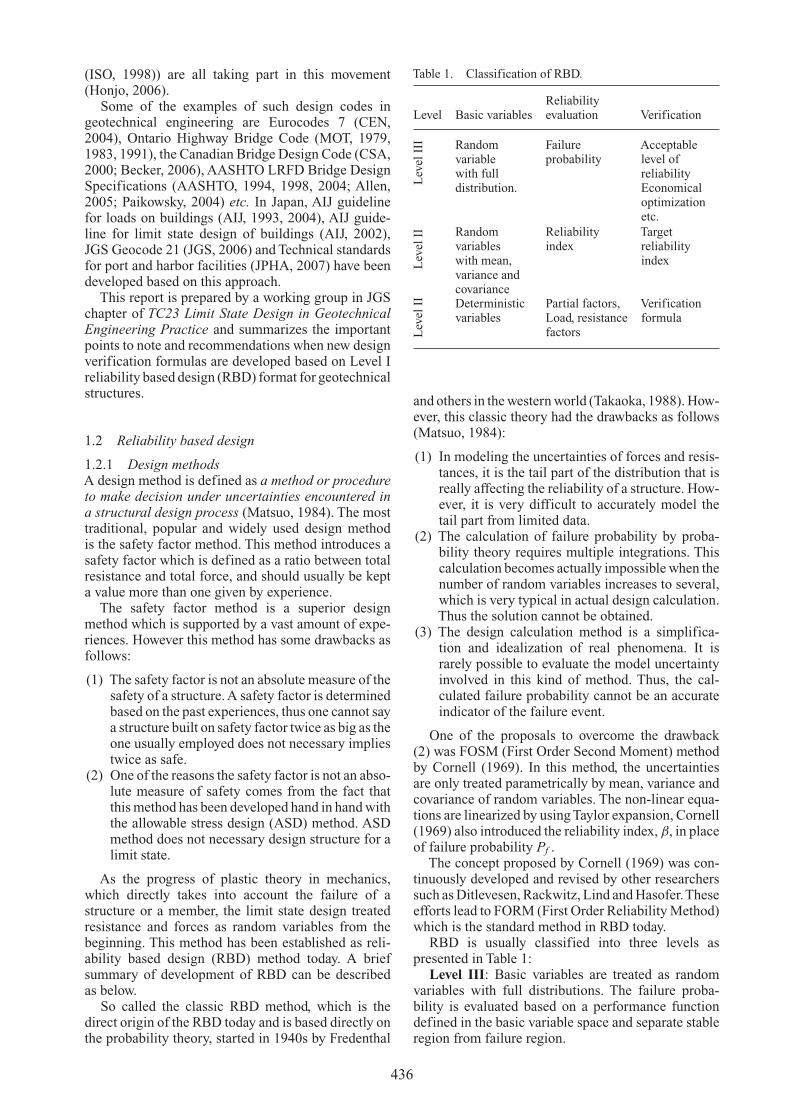
Table 1. Classification of RBD.

ReliabilityLevel Basic variables evaluation Verification

Random Failure Acceptablevariable probability level ofwith full reliabilitydistribution. Economical

optimizationetc.

Lev

elII

I

Random Reliability Targetvariables index reliabilitywith mean, indexvariance andcovariance

Lev

elII

Deterministic Partial factors, Verificationvariables Load, resistance formula

factorsLev

elII

and others in the western world (Takaoka, 1988). How-ever, this classic theory had the drawbacks as follows(Matsuo, 1984):

(1) In modeling the uncertainties of forces and resis-tances, it is the tail part of the distribution that isreally affecting the reliability of a structure. How-ever, it is very difficult to accurately model thetail part from limited data.

(2) The calculation of failure probability by proba-bility theory requires multiple integrations. Thiscalculation becomes actually impossible when thenumber of random variables increases to several,which is very typical in actual design calculation.Thus the solution cannot be obtained.

(3) The design calculation method is a simplifica-tion and idealization of real phenomena. It israrely possible to evaluate the model uncertaintyinvolved in this kind of method. Thus, the cal-culated failure probability cannot be an accurateindicator of the failure event.

One of the proposals to overcome the drawback(2) was FOSM (First Order Second Moment) methodby Cornell (1969). In this method, the uncertaintiesare only treated parametrically by mean, variance andcovariance of random variables. The non-linear equa-tions are linearized by using Taylor expansion, Cornell(1969) also introduced the reliability index, β, in placeof failure probability Pf .

The concept proposed by Cornell (1969) was con-tinuously developed and revised by other researcherssuch as Ditlevesen, Rackwitz, Lind and Hasofer.Theseefforts lead to FORM (First Order Reliability Method)which is the standard method in RBD today.

RBD is usually classified into three levels aspresented in Table 1:

Level III: Basic variables are treated as randomvariables with full distributions. The failure proba-bility is evaluated based on a performance functiondefined in the basic variable space and separate stableregion from failure region.

436

Level II: A simplified version of Level III. Basicvariables are parametrically described by mean, vari-ance and covariance. A method such as FORM is usedto evaluate the reliability index.

Level I: Necessary safety margin is preserved byapplying partial factors to characteristic values of basicvariables directly (i.e. PFM) or to calculated forcesand resistances (i.e. LRFD). All the calculations aredone deterministically, and a designer needs not tohave knowledge in reliability theory. However, codewriters need to determine the factors based on relia-bility analysis. The method is sometimes called limitstate design (LSD) and many design codes are nowbeing revised to this format.

1.2.2 Design methods and design codesA design code is a guideline document that describesprocedure of design for general and routinely designedstructures so that certain level of technical qualityis assured (Ovesen, 1989, 1993). Therefore, most ofthe structures we see daily are designed and builtaccording to design codes, and this fact reflects us theimportance of design codes.

As explained in the previous section, many designcodes in the world today are in the process of revisionfrom traditional ASD to LSD or Level I RBD. Some ofthe features of Level I RBD can be listed as follows:

(1) Reliability of a structure is evaluated based on socalled a limit state of a structure, a criterion that sep-arates desirable state (e.g. stable condition) fromundesirable state (e.g. failure). The ultimate andthe serviceability limit states are examples of thetypical limit states employed in RBD.

(2) The uncertainties involved in basic variables con-cerning actions, material properties, shape and size,etc. are taken care by factors which are determinedbased on reliability analyses. However, generalusers of these factors are not required to understandthe details of the reliability analyses.

(3) The harmonization of design codes is possibleunder identical concept.Traditionally, design codesare developed in different ways among differentstructures (e.g. buildings vs. bridges), and differ-ent materials (e.g. steel, concrete, composite, woodand geotechnical).

ISO documents such as ISO2394 General prin-ciples on reliability of structures (ISO, 1998) playsimportant role in the code development becauseWTO/TBT agreement requires for the member coun-tries to respect the internationally agreed standards.

Although most of the important parts of RBD havebeen developed by structural engineers as explainedin the previous section, geotechnical RBD also hassome original developments (Meyerhof, 1993). It isnatural for engineers to invent methods to encounteruncertainties while they carry out design in their ownways.

The most significant contribution of geotechnicalRBD came from Brinch Hansen (1953, 1956, 1967).He was the first person who used limit states in

geotechnical engineering and proposed to introducepartial safety factors into design codes. Under hisinfluence, a geotechnical design code using partialsafety factors has been established in Denmark since1965. Thus, LSD became much popular in Scandi-navian countries in early years, which added somedifferent background to Eurocode 7 compared to otherparts of the Structural Eurocodes.

One of the most well known structural reliabil-ity scholars, Ove Ditlevsen, states in his structuralreliability textbook that

A consistent code formulation of a detailed par-tial safety factor principle was started in the1950’s in Denmark before other places in theworld. This development got particular supportfrom the considerations of J. Brinch Hansenwho applied the principles in the field of soilmechanics. (Ditlevsen and Madsen, 1996, p.31)

It is understood that contribution of Brinch Hansenhas been recognized widely.

One of new trends concerning design codes is upriseof Performance based Design (PBD) concept, whichrequires transparency and accountability in design(Honjo & Kusakabe, 2002; Honjo et al., 2005). RBD(or LSD) seems to be the only rational tool to providea design verification procedure that designs a struc-ture for clearly defined limit states (i.e. performancesof structures and members) and introduces sufficientsafety margin. It is concluded that RBD will be usedas a tool to develop design codes at least for the nextseveral decades.

2 FORMAT OF VERIFICATION FORMULA

2.1 PFM vs. LRFD

The definitions of partial factor method (PFM) andload and resistance factor design (LRFD) in this reportare given in the following subsections:

2.1.1 PFMThe basic philosophy of this format is to treat the uncer-tainties at their origin. Thus many partial factors areintroduced in this format, which can be written as:

where, γri: partial factor multiplying to basic variablesxri in resistance side of the equation; γsi: partial fac-tor multiplying to basic variable xsi in load side. γRi′and γSi′ , another important group of partial factorsneed to be introduced to cover design modeling error,redundancy, brittleness, and statistical uncertainties.

It should be noticed that, partial factors for materialproperties are introduced to encounter against materialuncertainty, and a characteristic value of a material isusually discounted by a material partial factor beforeit is inserted to a design equation to calculate theresistance.

437

2.1.2 LRFDThe resistance and the load (external action) are firstcalculated based on the characteristic values of thebasic variables, then load and resistance factors areapplied to resulting resistance and load components toassure appropriate safety margin.

It may be convenient to list two types of LRFDformat as below:

where, γR: a resistance factor and γSj: a load factor fora load component Sj

where, γRi: resistance factors for resistance compo-nents Ri and γSj: load factors for load components Sj .

In Eq. (3), the resistance side maybe decomposedinto several lump sums that can be superimposed toobtain the final resistance (for example, pile tip andside resistances). Different resistance factors may beapplied to the different terms. This approach is some-times called MLRFD – Multiple Load and ResistanceFactor Design – (Phoon et al. 1995, Kulhawy andPhoon, 2002).

Traditionally, PFM is developed mainly inEurope(Gulvanessian and Holicky, 1996), whereasLRFD in the North America (Ellingwood et al., 1980,1982). However, they are mixedly used world widenow. In Eurocode 7 (CEN, 2004) and Geocode 21(JGS, 2006), Material Factor Approach (MFA) andResistance Factor Approach (RFA) are respectivelyused in almost the same way as PFM and LRFD here.

2.2 Pros and cones of PFM

PFM has advantages over LRFD on the followingaspects:

– It is intuitively felt reasonable to encounter uncer-tainties at their sources.

– It is easier to accommodate the development ofconstruction technique and design method whenthe uncertainties are treated at their origin: onecan simply change the partial factors related to theimprovement by the new developments.

However, it is very difficult to evaluate the reli-ability of structure by reliability analysis based onsuperposition of all uncertain sources for the followingreasons.

– Not all sources of uncertainties are known quan-titatively. Especially the model uncertainties aredifficult to evaluate.

– Some of the sources are correlated and difficult toconsider correlation in the reliability analysis.

– Sometimes overall uncertainty of the structure canbe estimated. However, it is difficult to break downthe result into each source.

– Many of the factors have non-linear effects on theresulting uncertainty of the structural reliability.Thus it is difficult to control the reliability of thestructure at the sources of uncertainties.

– Since PFM modifies the material property thatneeds to be input to the design calculation beforethe calculation, the actual behavior of structurebased on this calculation can be far from real-ity (or the most likely behavior). It is consideredthat, especially in geotechnical design where theengineering judgment plays very important role,such unrealistic calculation may not be favorable.In geotechnical design, there should be a philoso-phy that a designer should keep track of the mostlikely behavior of the structure toward the end ofthe design calculation as much as possible.

As could be suggested by the above discussion,although PFM looks theoretically sound, it encountersmany difficulties in practical situations. It is very diffi-cult, if not impossible, to rigorously determine partialfactors in practice.

2.3 Pros and cons of LRFD

Pros of PFM are cons of LRFD. However, LRFD issuperior to PFM in the following points:

– Especially for the resistance side, the design cal-culation based on LRFD predicts the most likelybehavior of the structure to its last stage of design,and it is in coincidence with the philosophy that adesigner should keep track of the most likely behav-ior of the structure to the last stage of the design asmuch as possible.

– In geotechnical design, where the interactionbetween a structure and ground is so high, it isnot possible to know whether the discount of thematerial parameter value may result safe design ofa structure. It is especially true for a sophisticateddesign calculation method like FEM.

– In many code calibration situations, uncertaintiesof a design method are provided as results of manyloading tests, for example in the form of database.The given uncertainties include all aspects of uncer-tainties, and it is impossible to decompose tovarious sources. Therefore, in practice, it is pos-sible to calibrate codes based on LRFD but not onPFM.

– LRFD has a design verification formula that ismore close to the traditional safety factor methodthan PFM. It may be easier for practical engineersto become familiar with LRFD than PFM.

For these reasons, LRFD is considered to be betterformat than PFM in geotechnical engineering designcode at least in the present situation.

3 DESIGN VALUE METHOD

3.1 General consideration on code calibrations

An engineer can design structures by using Level IRBD format without knowing the details of probability

438

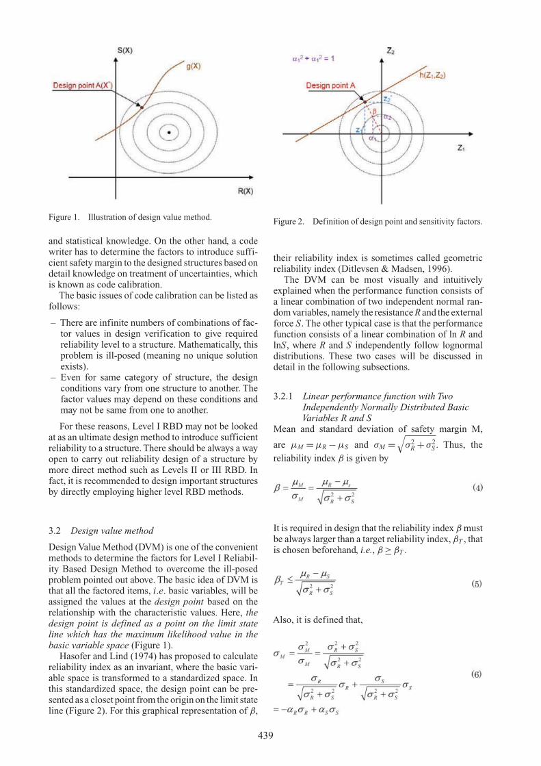
Figure 1. Illustration of design value method.

and statistical knowledge. On the other hand, a codewriter has to determine the factors to introduce suffi-cient safety margin to the designed structures based ondetail knowledge on treatment of uncertainties, whichis known as code calibration.

The basic issues of code calibration can be listed asfollows:

– There are infinite numbers of combinations of fac-tor values in design verification to give requiredreliability level to a structure. Mathematically, thisproblem is ill-posed (meaning no unique solutionexists).

– Even for same category of structure, the designconditions vary from one structure to another. Thefactor values may depend on these conditions andmay not be same from one to another.

For these reasons, Level I RBD may not be lookedat as an ultimate design method to introduce sufficientreliability to a structure. There should be always a wayopen to carry out reliability design of a structure bymore direct method such as Levels II or III RBD. Infact, it is recommended to design important structuresby directly employing higher level RBD methods.

3.2 Design value method

Design Value Method (DVM) is one of the convenientmethods to determine the factors for Level I Reliabil-ity Based Design Method to overcome the ill-posedproblem pointed out above. The basic idea of DVM isthat all the factored items, i.e. basic variables, will beassigned the values at the design point based on therelationship with the characteristic values. Here, thedesign point is defined as a point on the limit stateline which has the maximum likelihood value in thebasic variable space (Figure 1).

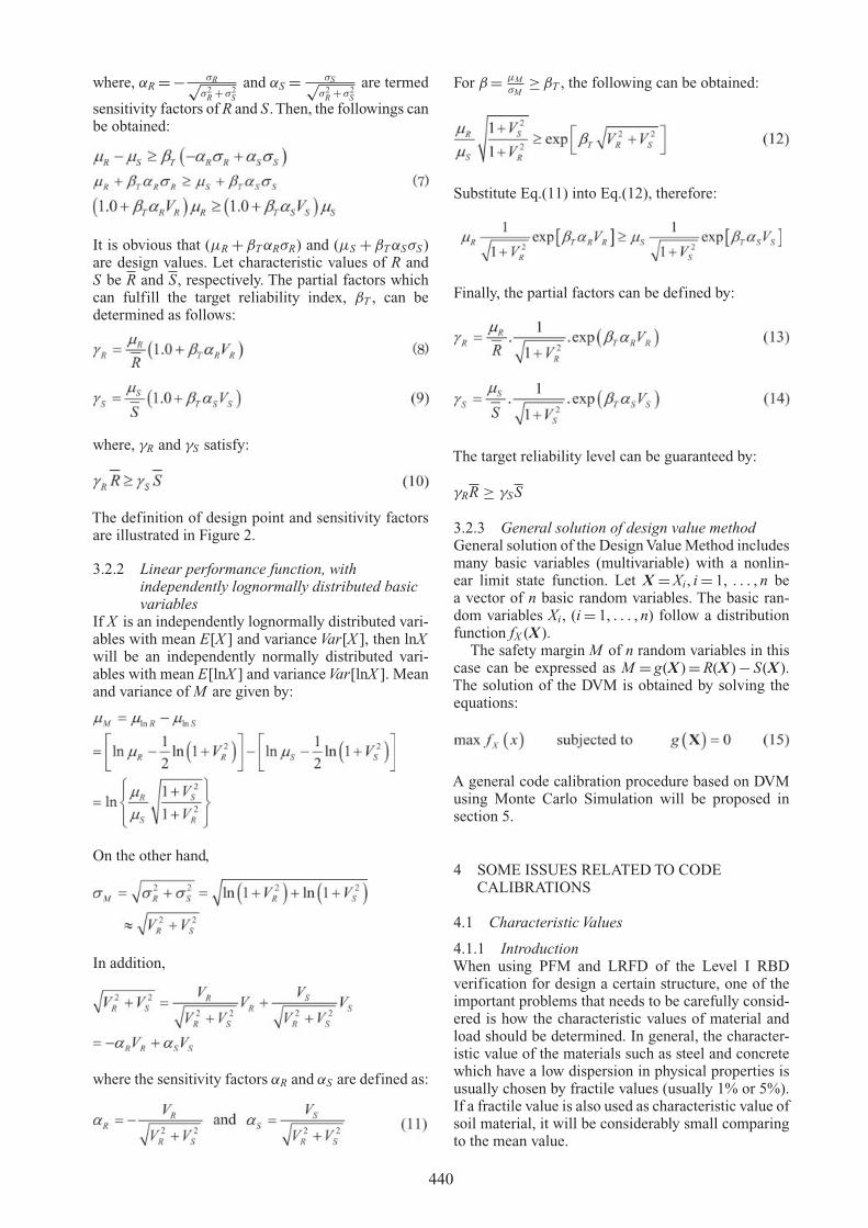
Hasofer and Lind (1974) has proposed to calculatereliability index as an invariant, where the basic vari-able space is transformed to a standardized space. Inthis standardized space, the design point can be pre-sented as a closet point from the origin on the limit stateline (Figure 2). For this graphical representation of β,

Figure 2. Definition of design point and sensitivity factors.

their reliability index is sometimes called geometricreliability index (Ditlevsen & Madsen, 1996).

The DVM can be most visually and intuitivelyexplained when the performance function consists ofa linear combination of two independent normal ran-dom variables, namely the resistance R and the externalforce S. The other typical case is that the performancefunction consists of a linear combination of ln R andlnS, where R and S independently follow lognormaldistributions. These two cases will be discussed indetail in the following subsections.

3.2.1 Linear performance function with TwoIndependently Normally Distributed BasicVariables R and S

Mean and standard deviation of safety margin M,

are μM = μR − μS and σM =√

σ2R + σ2

S . Thus, thereliability index β is given by

It is required in design that the reliability index β mustbe always larger than a target reliability index, βT , thatis chosen beforehand, i.e., β ≥ βT .

Also, it is defined that,

439

where, αR = − σR√σ2

R + σ2S

and αS = σS√σ2

R + σ2S

are termed

sensitivity factors of R and S. Then, the followings canbe obtained:

It is obvious that (μR + βT αRσR) and (μS + βT αSσS )are design values. Let characteristic values of R andS be R and S, respectively. The partial factors whichcan fulfill the target reliability index, βT , can bedetermined as follows:

where, γR and γS satisfy:

The definition of design point and sensitivity factorsare illustrated in Figure 2.

3.2.2 Linear performance function, withindependently lognormally distributed basicvariables

If X is an independently lognormally distributed vari-ables with mean E[X ] and variance Var[X ], then lnXwill be an independently normally distributed vari-ables with mean E[lnX ] and variance Var[lnX ]. Meanand variance of M are given by:

On the other hand,

In addition,

where the sensitivity factors αR and αS are defined as:

For β = μMσM

≥ βT , the following can be obtained:

Substitute Eq.(11) into Eq.(12), therefore:

Finally, the partial factors can be defined by:

The target reliability level can be guaranteed by:

γRR ≥ γSS

3.2.3 General solution of design value methodGeneral solution of the Design Value Method includesmany basic variables (multivariable) with a nonlin-ear limit state function. Let X = Xi, i = 1, . . . , n bea vector of n basic random variables. The basic ran-dom variables Xi, (i = 1, . . . , n) follow a distributionfunction fX (X ).

The safety margin M of n random variables in thiscase can be expressed as M = g(X ) = R(X ) − S(X ).The solution of the DVM is obtained by solving theequations:

A general code calibration procedure based on DVMusing Monte Carlo Simulation will be proposed insection 5.

4 SOME ISSUES RELATED TO CODECALIBRATIONS

4.1 Characteristic Values

4.1.1 IntroductionWhen using PFM and LRFD of the Level I RBDverification for design a certain structure, one of theimportant problems that needs to be carefully consid-ered is how the characteristic values of material andload should be determined. In general, the character-istic value of the materials such as steel and concretewhich have a low dispersion in physical properties isusually chosen by fractile values (usually 1% or 5%).If a fractile value is also used as characteristic value ofsoil material, it will be considerably small comparingto the mean value.

440

In a design calculation, if the output values propor-tionally change with the reduction of the input values(i.e. a linear model), whatever safety margin intro-duced in the input value is proportionally propagatedto the output. In design of foundation structures, how-ever, calculation of soil stress, bearing capacity etc.,follow highly non-linear models.

Furthermore, Finite Element Method and othernumerical calculation methods have been used broadlyand directly in geotechnical design. In these cases, ifthe characteristic value of a material used for design isconsiderably different from its mean value, the behav-ior of the designed structure will be far from the mostlikely behavior of the real structure. Also, consideringthe complex interaction among basic variables, it isimpossible to judge whether reduction of the mate-rial parameters would preserve safety of the wholestructure.

Simpson and Driscoll (1998) mentioned in theCommentary of Eurocode 7 that characteristic val-ues of geotechnical parameters are fundamental to allcalculations carried out in accordance with the code.Their definition has been the most controversial topicin the whole process of drafting Eurocode 7.

The characteristic value is usually equal to a cer-tain percentile of the distribution of that quantity (e.g.,mean, mode, median, mean minus one standard devia-tion, fractiles etc.). Whitman (1984) showed that someengineers use the mean value, while others used themost conservative of the measure strengths for thecharacteristic value.

According to the Eurocode 0, the nominal valuesfor resistance given by producers should correspond(at least approximately) to certain fractiles. For exam-ple, for steel structures, the values for resistance sideshould correspond to the 5%-fractile. In the case ofaction side, the characteristic values are defined asthe 50%-fractile (mean value) for permanent actions;98%-fractile of the distribution of the annual extremes,which means an average return period of 50 years forvariable actions (e.g. climatic actions).

4.1.2 Characteristic value in Eurocode 7Numerous debates on choice of the appropriate char-acteristic value for geotechnical design have beendone related to the development of Eurocode 7. Thesemethods can be listed such as statistical method inEurocode 7, method proposed by Schneider (1997),Bayesian approach, etc. However, the selection of thecharacteristic value is still open for debate betweenengineers. In Eurocode 7, the characteristic values ofloads and resistance are chosen as explained in detailedby Orr (2000).

(1) Characteristic value of loadsThe characteristic values of permanent loads derivedfrom the weights of materials, including water pres-sures, are normally selected using average or nominalunit weights for the materials, with no account beingtaken of the variability in unit weight. Characteris-tic earth pressures are obtained using characteristic

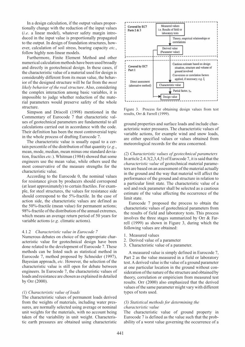
Figure 3. Process for obtaining design values from testresults, Orr & Farrell (1999).

ground properties and surface loads and include char-acteristic water pressures. The characteristic values ofvariable actions, for example wind and snow loads,are either specified values or values obtained frommeteorological records for the area concerned.

(2) Characteristic values of geotechnical parametersIn article 2.4.3(2,3,4,5) of Eurocode 7, it is said that thecharacteristic value of geotechnical material parame-ters are based on an assessment of the material actuallyin the ground and the way that material will affect theperformance of the ground and structure in relation toa particular limit state. The characteristic value of asoil and rock parameter shall be selected as a cautiousestimate of the value affecting the occurrence of thelimit state.

Eurocode 7 proposed the process to obtain thecharacteristic values of geotechnical parameters fromthe results of field and laboratory tests. This processinvolves the three stages summarized by Orr & Far-rell (1999) as shown in Figure 3, during which thefollowing values are obtained:

1. Measured values2. Derived value of a parameter3. Characteristic value of a parameter.

A measured value is simply defined in Eurocode 7,Part 2 as the value measured in a field or laboratorytest.A derived value is the value of a ground parameterat one particular location in the ground without con-sideration of the nature of the structure and obtained bytheory, correlation or empiricism from measured testresults. Orr (2000) also emphasized that the derivedvalues of the same parameter might vary with differenttypes of tests used.

(3) Statistical methods for determining thecharacteristic valueThe characteristic value of ground property inEurocode 7 is defined as the value such that the prob-ability of a worst value governing the occurrence of a

441

limit state is not greater than 5%, i.e. 95% confidencelevel that the actual mean value is greater than theselected characteristic value. Eurocode 7 also empha-size that the statistical method should be comparedto the results obtained by Bayesian method instead ofusing only pure statistical approach without consid-eration on the actual design situation and comparableexperience.

The characteristic value, X of a soil property instatistical method is given by:

where μX is mean value, kn is a factor, dependingon the type of statistical distribution and the numberof test results, and VX is the coefficient of variation.Since the actual mean value, μX of a soil parametercannot normally be determined statistically by a suf-ficient number of tests, it must be assessed from theaverage value, �

μX of the test results.One way to obtain the factor kn in the above equation

is using pseudonym of Student proposed by Gossett.Orr (2000) also noticed that the characteristic valueobtained by statistical method using Student t valuewill become too cautious and uneconomic in case oflimited number of test results which is common inpractice.

(4) Schneider’s method for determining thecharacteristic valueBased on comparative calculations, Schneider (1997)has shown that a good approximation to X is obtainedwhen kn = 0.5, i.e. if the characteristic value is chosenas one half a standard deviation below the mean valueas in the following equation:

where the mean, standard deviation and coefficient ofvariation are obtained from test results.

(5) Bayesian approach for determining thecharacteristic valueThis approach may be used to determine the char-acteristic value when some comparable experience isavailable that enables the mean and standard deviationvalues to be estimated. In this situation, it is possible tocombine the test results with the estimated values, i.e.a priori values, using Bayes’ theorem so as to obtainmore reliable mean and standard deviation values andhence a more reliable characteristic value.The relevantequations for the mean and standard deviation usingthe Bayesian approach are (Tang, 1971):

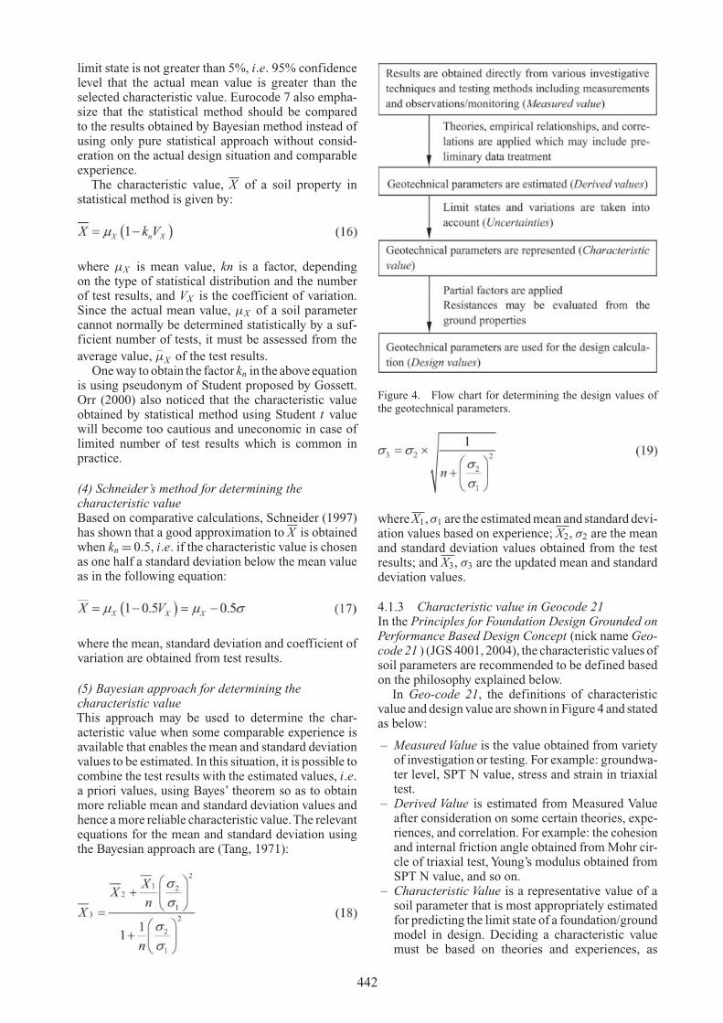
Figure 4. Flow chart for determining the design values ofthe geotechnical parameters.

where X1, σ1 are the estimated mean and standard devi-ation values based on experience; X2, σ2 are the meanand standard deviation values obtained from the testresults; and X3, σ3 are the updated mean and standarddeviation values.

4.1.3 Characteristic value in Geocode 21In the Principles for Foundation Design Grounded onPerformance Based Design Concept (nick name Geo-code 21 ) (JGS 4001, 2004), the characteristic values ofsoil parameters are recommended to be defined basedon the philosophy explained below.

In Geo-code 21, the definitions of characteristicvalue and design value are shown in Figure 4 and statedas below:

– Measured Value is the value obtained from varietyof investigation or testing. For example: groundwa-ter level, SPT N value, stress and strain in triaxialtest.

– Derived Value is estimated from Measured Valueafter consideration on some certain theories, expe-riences, and correlation. For example: the cohesionand internal friction angle obtained from Mohr cir-cle of triaxial test, Young’s modulus obtained fromSPT N value, and so on.

– Characteristic Value is a representative value of asoil parameter that is most appropriately estimatedfor predicting the limit state of a foundation/groundmodel in design. Deciding a characteristic valuemust be based on theories and experiences, as

442

well as sufficiently consider the dispersion of soilparameters and the applicability of the simplifiedmodel.

Geo-code 21 defined the characteristic value asfollow:

The characteristic value of a geotechnicalparameter is principally thought of as the aver-age (expected value) of the derived values. It is nota mere mathematical average, but also accountsfor the estimation errors associated with statisticalaveraging. Moreover, the average value shall becarefully and comprehensively chosen consideringdata from past geologic/geotechnical engineering,experiences with similar projects, and relation-ships and consistencies among the results of differ-ent geotechnical investigations and tests. (Designprinciple 2.4.3(c))

– Design Value is the value of foundation parameterthat is used in design calculation model in case ofmaterial factor approach and can be obtained byapplying partial factor to characteristic value.

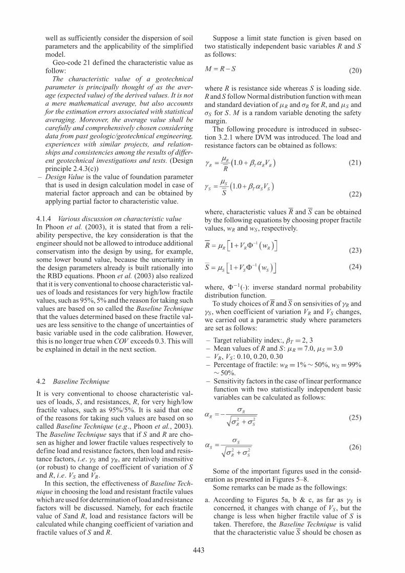
4.1.4 Various discussion on characteristic valueIn Phoon et al. (2003), it is stated that from a reli-ability perspective, the key consideration is that theengineer should not be allowed to introduce additionalconservatism into the design by using, for example,some lower bound value, because the uncertainty inthe design parameters already is built rationally intothe RBD equations. Phoon et al. (2003) also realizedthat it is very conventional to choose characteristic val-ues of loads and resistances for very high/low fractilevalues, such as 95%, 5% and the reason for taking suchvalues are based on so called the Baseline Techniquethat the values determined based on these fractile val-ues are less sensitive to the change of uncertainties ofbasic variable used in the code calibration. However,this is no longer true when COV exceeds 0.3. This willbe explained in detail in the next section.

4.2 Baseline Technique

It is very conventional to choose characteristic val-ues of loads, S, and resistances, R, for very high/lowfractile values, such as 95%/5%. It is said that oneof the reasons for taking such values are based on socalled Baseline Technique (e.g., Phoon et al., 2003).The Baseline Technique says that if S and R are cho-sen as higher and lower fractile values respectively todefine load and resistance factors, then load and resis-tance factors, i.e. γS and γR, are relatively insensitive(or robust) to change of coefficient of variation of Sand R, i.e. VS and VR.

In this section, the effectiveness of Baseline Tech-nique in choosing the load and resistant fractile valueswhich are used for determination of load and resistancefactors will be discussed. Namely, for each fractilevalue of Sand R, load and resistance factors will becalculated while changing coefficient of variation andfractile values of S and R.

Suppose a limit state function is given based ontwo statistically independent basic variables R and Sas follows:

where R is resistance side whereas S is loading side.R and S follow Normal distribution function with meanand standard deviation of μR and σR for R, and μS andσS for S. M is a random variable denoting the safetymargin.

The following procedure is introduced in subsec-tion 3.2.1 where DVM was introduced. The load andresistance factors can be obtained as follows:

where, characteristic values R and S can be obtainedby the following equations by choosing proper fractilevalues, wR and wS , respectively.

where, �−1(·): inverse standard normal probabilitydistribution function.

To study choices of R and S on sensivities of γR andγS , when coefficient of variation VR and VS changes,we carried out a parametric study where parametersare set as follows:

– Target reliability index:, βT = 2, 3– Mean values of R and S: μR = 7.0, μS = 3.0– VR, VS : 0.10, 0.20, 0.30– Percentage of fractile: wR = 1% ∼ 50%, wS = 99%

∼ 50%.– Sensitivity factors in the case of linear performance

function with two statistically independent basicvariables can be calculated as follows:

Some of the important figures used in the consid-eration as presented in Figures 5–8.

Some remarks can be made as the followings:

a. According to Figures 5a, b & c, as far as γS isconcerned, it changes with change of VS , but thechange is less when higher fractile value of S istaken. Therefore, the Baseline Technique is validthat the characteristic value S should be chosen as

443

Figure 5(a). VS vs. γS, Normal, βT = 3, VR = 0.1.

Figure 5(b). VS vs. γS, Normal, βT = 3, VR = 0.2.

Figure 5(c). VS vs. γS, Normal, βT = 3, VR = 0.3.

a higher fractile value, for example 95% or 99%.It should be noticed, however, that if one takes avery high fractile value, one may get a load fac-tor, γS , that is smaller than unity (Figures 6a, b, &c). This may not be preferable for practical designengineers.

b. However, for γR, the advantage of Baseline Tech-nique is not as obvious as that for γS . As can beseen from Figures 7a, b, & c, stability of γR forlower fractile values is not so obvious as that ofvalues closer to mean value.Furthermore, γR is very unstable to change of VRwhen a very low fractile value is taken. The samestatement can be read from Figures 8a, b, & c thatγR’s for different VR are not getting closer for smallfractile value of R.

c. The statements (a) and (b) are more pronouncedwhen βT is larger, although the results are notattached in this paper.

Therefore, for the case with two independently sta-tistically normally-distributed random variables SandRin the linear performance function M = R–S, it is rec-ommended to take high fractile value for S, however,

Figure 6(a). wS vs. γS, Normal, βT = 3, VR = 0.1.

Figure 6(b). wS vs. γS, Normal, βT = 3, VR = 0.2.

Figure 6(c). wS vs. γS, Normal, βT = 3, VR = 0.3.

using the low fractile value for R may not be as effectiveas in case of S.

The same procedure is also done for the casethat Sand Rfollow lognormal distributions. It is alsoobserved that the Baseline Technique is valid for Sthan for R when S and R follow lognormal distribu-tions. Furthermore, compared to the normal case, allthe statements are more pronounced in lognormal case.

In conclusion, the advantage of Baseline Techniqueis much more obvious in determining the load factor,γS , comparing to that of γR. It is recommended to takehigh fractile value for S, however the low fractile valueneed not to be chosen for R.

4.3 Determination of a target reliability

As introduced in many references and textbooks, thereare mainly three ways to determine a target reliabilitylevel:

(1) Adopt reliability level that preserved in the exist-ing structures. This implies preserve the reliabilitylevel of the existing design codes.

444

Figure 7(a). VR vs. γR, Normal, βT = 3, VS = 0.1.

Figure 7(b). VR vs. γR, Normal, βT = 3, VS = 0.2.

Figure 7(c). VR vs. γR, Normal, βT = 3, VS = 0.3.

Figure 8(a). wR vs. γR, Normal, βT = 3, VS = 0.1.

(2) Determine the reliability level based on compari-son with other existing individual and social risks,i.e. the background risks.

(3) Use optimization scheme based on some economicor other criteria (e.g. LQI).

The methods are ordered from simple and practicalones to more theoretical and ideal ones. In the actualcode calibration, the first method is mostly employed.The information obtained in the second is useful when

Figure 8(b). wR vs. γR, Normal, βT = 3, VS = 0.2.

Figure 8(c). wR vs. γR, Normal, βT = 3, VS = 0.3.

one needs to compare the design reliability risk to othersocial risks. This situation is coming to be importantwhen one needs to make decision between infrastruc-ture building and other soft alternatives. For the lastmethod, it may be important to understand the gen-eral framework of the method. However, this method israrely used in practical code calibration, and discardedfrom this report.

4.3.1 Target reliability by existing design codesDue to various difficulties in evaluating absolute levelof reliability of designed structure, most of practicalcode calibrations are done by setting target reliabilitylevel based on existing structures assuming that theexisting structures are satisfying the reliability levelrequired by the society.

Common practice is to evaluate the reliability levelof the existing structure before setting the target reli-ability level. This implies the reliability analysis ofstructures designed by the existing design codes.

For the convenience of code writers, some typicaltarget reliability indices, βT, are listed in a documentlike ISO2394 (ISO, 1998). ISO2394 first gives therelationship between β and failure probability assum-ing β follows the normal distribution as shown inTable2. The typical target reliability indices are presented inTable 3.

AISC LRFD (Elingwood et al., 1980, 1982) whichis LRFD based code adopted target β to be 2.5–3.5 forsteel beams and columns, and 3.0–3.5 for RC beamsand columns. This was one of the first attempts tocalibrate load and resistance factors in LRFD baseddesign code.

445

Table 5. Relationship between β and Pf .

Pf 10−1 10−2 10−3 10−4 10−5 10−6 10−7

β 1.3 2.3 3.1 3.7 4.2 4.7 5.2

Table 6. Taget β-values (life-time, examples).

Relative costs of Consequences of failuresafety measures

small some moderate great

High 0 A 1.5 2.3 B 3.1Moderate 1.3 2.3 3.1 C 3.8Low 2.3 3.1 3.8 4.3

Some suggestions are:A: for serviceability limit sates, use β = 0 for reversibleand β = 1.5 for irreversible limit sate.B: for fatigue limit states, use β = 2.3 to 3.1,depending on the possibility of inspections.C: for ultimate limit states design, use the safetyclasses β = 3.1, 3.8 and 4.3.

The target β’s that have been used in geotechnicalcode calibrations have been summarized in Paikowsky(2004). Based on the review, they adopted the targetβ? for a single pile to be 3.0, whereas 2.33 is used forgroup piles supporting a foundation with more than 5piles. The reduced β was adopted in the group pilesbecause of the redundancy of the foundation system.

There are many proposed target β in the variousreports and papers. It is, however, important to care-fully review the purpose for which the target β is set.They may be different for material, members, failuremodes, limit states and calculation methods. Further-more, β can be defined either for annual or for lifetime of a structure, and distinction between the two issometimes overlooked.

4.3.2 Criteria on allowable riskICG (2003) defines risk as probability of an eventtimes consequence if the event occurs. Similar defi-nitions of risk can be found in many other literatures(e.g. Beacher & Christian, 2003). Therefore it isimportant to consider both probability (i.e. frequency)of the occurrence of event and its consequence at thesame time. Furthermore, in preparing countermea-sures for reducing risk, both reduction of frequencyand consequence need to be considered.

It is not appropriate to think there is an absolutethreshold between acceptable risk and unacceptablerisk. Every individual has his/her own preferencefor risk, and therefore acceptable risk level is dif-ferent from a person to another depending on therisk under consideration. Starr (1969) has pointed outthat there is quite difference between acceptable lev-els for involuntary and voluntary risks. Slovic (1987)found that factors like dread or uncontrollable andunknown or unobservable influence considerably inrisk recognition of general individuals.

In order to accommodate such ambiguity in accept-able risk level recognition into account, HSE (1999) ofUK proposed to divide risk levels into three regions:

(1) Unacceptable region: risk cannot be justifiedexcept in extraordinary circumstances.

(2) ALARP (as low as reasonably possible) region:tolerable only if the cost of risk reduction is grosslydisproportionate to the reduction in risk achieved.

(3) Risk negligible region: further effort to reduce riskis not normally necessary.

ALARP region is well established in case law inUK, and has been adopted in UK health and safetyAct (GEO, 2007; Diamantidis, 2008).

Diamantidis (2008) has proposed to make dis-tinction between individual risk and societal risk indeveloping criteria for acceptable risk level, which isalso followed in the report.

(1) Individual riskIndividual risk is defined as the annual probability

of being harmed by a hazardous situation. A typicalindividual risk is fatality risk which can be measuredby the annual probability of being killed by some harm.Table 7 presents annual fatal accident rate in the devel-oped countries by Diamantidis (2008). In addition,annual fatal accident rate in Japan derived from officialstatistics in 2004 in Japan by Honjo (2006) are pre-sented in Table 8. Some of the figures are also copiedto Table 7 for comparison. It should be noticed that themethods used to obtain these rates in these two tablesare different, thus comparison may be made with somecare.

It may be possible to say from these results that therisk level for each event is different whether they arevoluntary or involuntary, and also benefit one can getfrom each event.

(2) Societal riskOne of the most popular ways to describe the

societal risk is by an F–N curve. F stands for fre-quency and N for number of fatalities. An F–Ncurve presents probability of occurrence of an acci-dent which involves more than n fatalities, and hasrelationship with the cumulative distribution functionof N as follows:

F–N curve was widely known by a report prepared byUSNRC(1975), known as Wash 1400, to show the riskof building nuclear power plants in US. F–N curvesshowing various societal risks with the risk of oper-ating nuclear power plants were presented in order tojustify the construction of new nuclear power plantsin the US. In the field of geotechnical engineering, anF–N curve drawn by Baecher in 1982 is well known(Baecher & Christian, 2003).

Some of relatively new F−N curves proposed in thevarious parts of the world have been plotted in Figure 9.These are the Dutch government published risk guide-lines (Versteeg, 1987), the Hong Kong governmentplanning department (HKPD, 1994) and ANCOLD

446

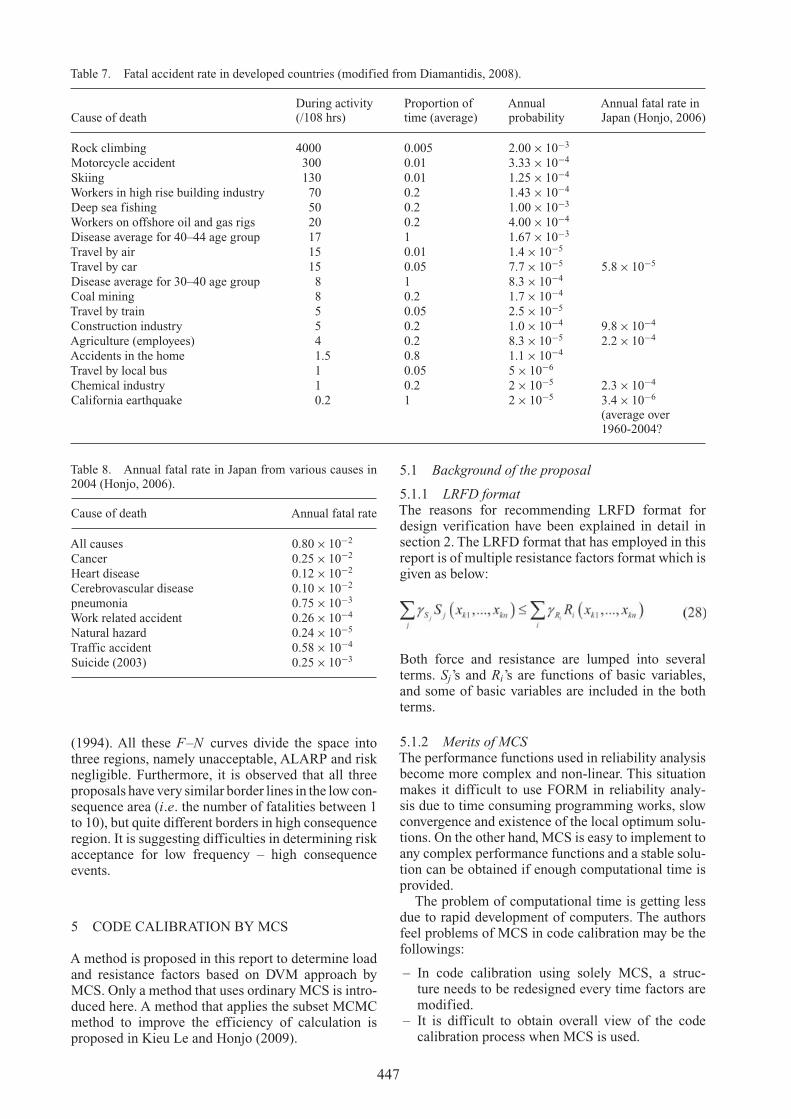
Table 7. Fatal accident rate in developed countries (modified from Diamantidis, 2008).

During activity Proportion of Annual Annual fatal rate inCause of death (/108 hrs) time (average) probability Japan (Honjo, 2006)

Rock climbing 4000 0.005 2.00 × 10−3

Motorcycle accident 300 0.01 3.33 × 10−4

Skiing 130 0.01 1.25 × 10−4

Workers in high rise building industry 70 0.2 1.43 × 10−4

Deep sea fishing 50 0.2 1.00 × 10−3

Workers on offshore oil and gas rigs 20 0.2 4.00 × 10−4

Disease average for 40–44 age group 17 1 1.67 × 10−3

Travel by air 15 0.01 1.4 × 10−5

Travel by car 15 0.05 7.7 × 10−5 5.8 × 10−5

Disease average for 30–40 age group 8 1 8.3 × 10−4

Coal mining 8 0.2 1.7 × 10−4

Travel by train 5 0.05 2.5 × 10−5

Construction industry 5 0.2 1.0 × 10−4 9.8 × 10−4

Agriculture (employees) 4 0.2 8.3 × 10−5 2.2 × 10−4

Accidents in the home 1.5 0.8 1.1 × 10−4

Travel by local bus 1 0.05 5 × 10−6

Chemical industry 1 0.2 2 × 10−5 2.3 × 10−4

California earthquake 0.2 1 2 × 10−5 3.4 × 10−6

(average over1960-2004?

Table 8. Annual fatal rate in Japan from various causes in2004 (Honjo, 2006).

Cause of death Annual fatal rate

All causes 0.80 × 10−2

Cancer 0.25 × 10−2

Heart disease 0.12 × 10−2

Cerebrovascular disease 0.10 × 10−2

pneumonia 0.75 × 10−3

Work related accident 0.26 × 10−4

Natural hazard 0.24 × 10−5

Traffic accident 0.58 × 10−4

Suicide (2003) 0.25 × 10−3

(1994). All these F–N curves divide the space intothree regions, namely unacceptable, ALARP and risknegligible. Furthermore, it is observed that all threeproposals have very similar border lines in the low con-sequence area (i.e. the number of fatalities between 1to 10), but quite different borders in high consequenceregion. It is suggesting difficulties in determining riskacceptance for low frequency – high consequenceevents.

5 CODE CALIBRATION BY MCS

A method is proposed in this report to determine loadand resistance factors based on DVM approach byMCS. Only a method that uses ordinary MCS is intro-duced here. A method that applies the subset MCMCmethod to improve the efficiency of calculation isproposed in Kieu Le and Honjo (2009).

5.1 Background of the proposal

5.1.1 LRFD formatThe reasons for recommending LRFD format fordesign verification have been explained in detail insection 2. The LRFD format that has employed in thisreport is of multiple resistance factors format which isgiven as below:

Both force and resistance are lumped into severalterms. Sj’s and Ri’s are functions of basic variables,and some of basic variables are included in the bothterms.

5.1.2 Merits of MCSThe performance functions used in reliability analysisbecome more complex and non-linear. This situationmakes it difficult to use FORM in reliability analy-sis due to time consuming programming works, slowconvergence and existence of the local optimum solu-tions. On the other hand, MCS is easy to implement toany complex performance functions and a stable solu-tion can be obtained if enough computational time isprovided.

The problem of computational time is getting lessdue to rapid development of computers. The authorsfeel problems of MCS in code calibration may be thefollowings:

– In code calibration using solely MCS, a struc-ture needs to be redesigned every time factors aremodified.

– It is difficult to obtain overall view of the codecalibration process when MCS is used.

447

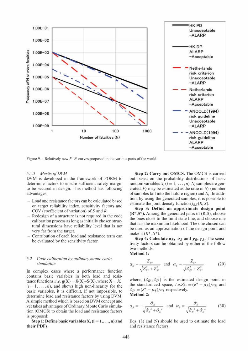
Figure 9. Relatively new F–N curves proposed in the various parts of the world.

5.1.3 Merits of DVMDVM is developed in the framework of FORM todetermine factors to ensure sufficient safety marginto be secured in design. This method has followingadvantages:

– Load and resistance factors can be calculated basedon target reliability index, sensitivity factors andCOV (coefficient of variation) of S and R.

– Redesign of a structure is not required in the codecalibration process as long as initially chosen struc-tural dimensions have reliability level that is notvery far from the target.

– Contribution of each load and resistance term canbe evaluated by the sensitivity factor.

5.2 Code calibration by ordinary monte carlosimulation

In complex cases where a performance functioncontains basic variables in both load and resis-tance functions, i.e. g(X) = R(X)–S(X), where X = Xi,(i = 1, . . . , n), and shows high non-linearity for thebasic variables, it is difficult, if not impossible, todetermine load and resistance factors by using DVM.A simple method which is based on DVM concept andyet takes advantages of Ordinary Monte Carlo simula-tion (OMCS) to obtain the load and resistance factorsis proposed:

Step 1:Define basic variables Xi (i = 1,. . .,n) andtheir PDFs.

Step 2: Carry out OMCS. The OMCS is carriedout based on the probability distributions of basicrandom variables Xi (i = 1, . . . , n). Nt samples are gen-erated. Pf may be estimated as the ratio of Nf (numberof samples fall into the failure region) and Nt . In addi-tion, by using the generated samples, it is possible toestimate the joint density function fR,S (R, S).

Step 3: Define an approximate design point(R*,S*). Among the generated pairs of (R,S), choosethe ones close to the limit state line, and choose onethat has the maximum likelihood. The one chosen canbe used as an approximation of the design point andmake it (R*, S*).

Step 4: Calculate αR, αS and γR, γS . The sensi-tivity factors can be obtained by either of the followtwo methods:Method 1:

where, (ZR∗ , ZS∗ ) is the estimated design point inthe standardized space, i.e.ZR∗ = (R∗ − μR)/σR andZS∗ = (S∗ − μS)/σS respectively.Method 2:

Eqs. (8) and (9) should be used to estimate the loadand resistance factors.

448

Table 9. Sensitivity factors, load and resistance factorsobtained for simple linear performance function example.

αR αS γR γS

OMCS −0.72 0.69 0.67 1.12Subset MCMC −0.69 0.73 0.69 1.15True results −0.71 0.71 0.68 1.13

If it is judged more appropriate to fit lognormaldistribution, the sensitivity factors can be estimatedby either of the two methods as follows:Method 1’:

where, (ZlnR∗ , ZlnS∗ ) is the estimated design point instandardized space, i.e. Zln R∗ = ( ln R∗ − μln R)/σln Rand Zln S∗ = ( ln S∗ − ln μS)/ ln σS.Method 2’:

Eqs. (13) and (14) should be used to estimate theload and resistance factors.

5.3 Examples

5.3.1 Linear performance function Z = R − SR and S are independently normally distributed ran-dom variables, i.e. R ∼ N(7.0,1.0) and S ∼ N(3.0,1.0)(Kieu Le & Honjo, 2009).

In this example, the true results are known asfollows:

True failure probability: Pf = 0.23 × 10−2

True reliability index: β = 2.83True design point: (R∗, S∗) = (5.0,5.0)

In this example sensitivity factors obtained byMethod 1 (Eq.(29)) are true values. Load and resis-tance factors are then obtained for a certain targetreliability index, for example, βT = 3.2. The resultsare also shown in Table 9.

The results obtained by OMCS after 50,000 runsare as follows:

Probability of failure: Pf = 0.25 × 10−2

Reliability index: β = 2.81Design point: D(R∗, S∗) = (5.1,4. 8)

Sensitivity factors are calculated by using Method 2shown in Eq.(30), whereas the load and resistance fac-tors are obtained forβT = 3.2, and the results are shownin Table 9.

A similar procedure based on DVM and SubsetMCMC by Kieu Le & Honjo (2009) is also attemptedwith Nt = 100 samples. An example of the generatedsamples is shown in Figure 10.

Figure 10. Generated samples for simple linear perfor-mance function.

Probability of failure: Pf = 0.26 × 10−2

Reliability index: β = 2.79

The samples of the last step are used to estimate thedesign point.

Design point: D(R∗, S∗) = (5.1,5.0)

Sensitivity factors are calculated by using Method 2shown in Eq.(30). Finally, load and resistance factorsare obtained for βT = 3.2. The results are aslo shownin Table 9.

It may be recognized that the results obtained by theproposed method based on OMCS (or Subset MCMC)and DVM are very close to the true results. Therefore,the method seems to work well in this simple example.

5.3.2 A Retaining wall exampleDetermination of load and resistance factors

The proposed method is now applied for reliabil-ity analysis of a gravity retaining wall (Figure 11)under sliding failure mode(Kieu Le & Honjo, 2009).This example is taken from Orr (2005). The necessaryparameters of the retaining wall, soil below and fillabove the retaining wall are described below.

– Properties of sand beneath wall: c′s = 0, φ′

s, γs– Properties of fill behind wall: c′

f = 0, φ′f , γf

– Groundwater level is at depth below the base of thewall

– Friction angle between base wall and underlainsand: φ′

bs– Thickness of retaining wall: w = 0.4 m

The limit state function of the problem is given as:

where R: total horizontal force that resists horizontalmovement of the wall, S: total horizontal force thatmoves the wall.

449

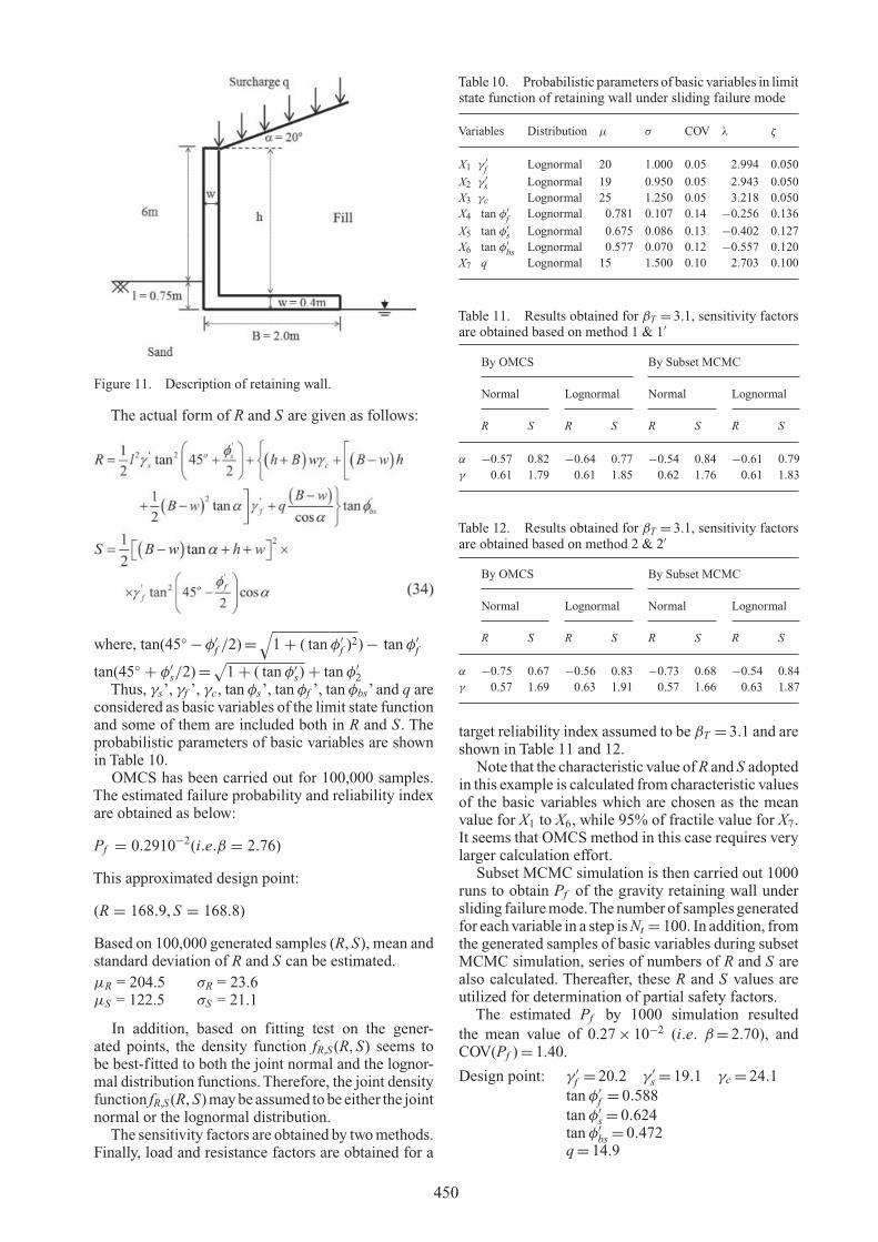
Figure 11. Description of retaining wall.

The actual form of R and S are given as follows:

where, tan(45◦ − φ′f /2) =

√1 + ( tan φ′

f )2) − tan φ′f

tan(45◦ + φ′s/2) = √

1 + ( tan φ′s) + tan φ′

2Thus, γs’, γf ’, γc, tan φs’, tan φf ’, tan φbs’ and q are

considered as basic variables of the limit state functionand some of them are included both in R and S. Theprobabilistic parameters of basic variables are shownin Table 10.

OMCS has been carried out for 100,000 samples.The estimated failure probability and reliability indexare obtained as below:

Pf = 0.2910−2(i.e.β = 2.76)

This approximated design point:

(R = 168.9, S = 168.8)

Based on 100,000 generated samples (R, S), mean andstandard deviation of R and S can be estimated.μR = 204.5 σR = 23.6μS = 122.5 σS = 21.1

In addition, based on fitting test on the gener-ated points, the density function fR,S (R, S) seems tobe best-fitted to both the joint normal and the lognor-mal distribution functions. Therefore, the joint densityfunction fR,S (R, S) may be assumed to be either the jointnormal or the lognormal distribution.

The sensitivity factors are obtained by two methods.Finally, load and resistance factors are obtained for a

Table 10. Probabilistic parameters of basic variables in limitstate function of retaining wall under sliding failure mode

Variables Distribution μ σ COV λ ζ

X1 γ ′f Lognormal 20 1.000 0.05 2.994 0.050

X2 γ ′s Lognormal 19 0.950 0.05 2.943 0.050

X3 γc Lognormal 25 1.250 0.05 3.218 0.050X4 tan φ′

f Lognormal 0.781 0.107 0.14 −0.256 0.136X5 tan φ′

s Lognormal 0.675 0.086 0.13 −0.402 0.127X6 tan φ′

bs Lognormal 0.577 0.070 0.12 −0.557 0.120X7 q Lognormal 15 1.500 0.10 2.703 0.100

Table 11. Results obtained for βT = 3.1, sensitivity factorsare obtained based on method 1 & 1′

By OMCS By Subset MCMC

Normal Lognormal Normal Lognormal

R S R S R S R S

α −0.57 0.82 −0.64 0.77 −0.54 0.84 −0.61 0.79γ 0.61 1.79 0.61 1.85 0.62 1.76 0.61 1.83

Table 12. Results obtained for βT = 3.1, sensitivity factorsare obtained based on method 2 & 2′

By OMCS By Subset MCMC

Normal Lognormal Normal Lognormal

R S R S R S R S

α −0.75 0.67 −0.56 0.83 −0.73 0.68 −0.54 0.84γ 0.57 1.69 0.63 1.91 0.57 1.66 0.63 1.87

target reliability index assumed to be βT = 3.1 and areshown in Table 11 and 12.

Note that the characteristic value of R and S adoptedin this example is calculated from characteristic valuesof the basic variables which are chosen as the meanvalue for X1 to X6, while 95% of fractile value for X7.It seems that OMCS method in this case requires verylarger calculation effort.

Subset MCMC simulation is then carried out 1000runs to obtain Pf of the gravity retaining wall undersliding failure mode.The number of samples generatedfor each variable in a step is Nt = 100. In addition, fromthe generated samples of basic variables during subsetMCMC simulation, series of numbers of R and S arealso calculated. Thereafter, these R and S values areutilized for determination of partial safety factors.

The estimated Pf by 1000 simulation resultedthe mean value of 0.27 × 10−2 (i.e. β = 2.70), andCOV(Pf ) = 1.40.

Design point: γ ′f = 20.2 γ ′

s = 19.1 γc = 24.1tan φ′

f = 0.588tan φ′

s = 0.624tan φ′

bs = 0.472q = 14.9

450

This approximated design point is equivalent to point(R = 169.1, S = 166.8).

Nt pairs of (R, S) calculated from Nt generatedpoints Xi (i = 1, . . . , n), that are generated in the subsetF0, are utilized to estimate mean and standard devia-tion of R and S. The joint density function fR,S (R, S)is also assumed to be either the joint normal or thelognormal distribution.μR = 201.1 σR = 21.8μS = 120.8 σS = 20.2

The sensitivity factors are obtained by two methods.Load and resistance factors (shown inTable 11 and 12.)are obtained for the same βT and the characteristicvalue of R and S as in the case of OMCS.

Followings are some remarks on the results:

– Load and Resistance Factors obtained all the cases,i.e. different joint density functions, different wayto calculate sensitivity factors, are very similar.

– The results obtained based on the estimated designpoint in Table 11 (by method 1 & 1’) is better thanthose obtained based on only the samples generatedin the first step of subset MCMC procedure inTable12 (method 2 & 2’), as expected.

– The results obtained by OMCS (for 100,000 sam-ples) and Subset MCMC are quite similar.

6 SUMMARY AND CONCLUSIONS

This report is prepared by a working group in JGSchapter of TC23 Limit State Design in Geotechni-cal Engineering Practice and summarizes the impor-tant points to note and recommendations when newdesign verification formulas are developed based onLevel I RBD format. The followings are the majorrecommendations of this report.

(1) Several RBD Level I verification formats such asPFM and LRFD have been proposed. It is recom-mended to use LRFD format at present due to thereasons below:-A designer can trace the most likely behavior ofthe structure to the very last stage of design ifthe characteristic values of the resistance basicvariables are appropriately chosen.-The format can accommodate a performancefunction with high non-linearity and with somebasic variables to both force and resistance sides.-Code calibration is possible for the case onlytotal uncertainty of the design method is known,where the total uncertainty cannot be decomposedto each source of uncertainty.

(2) The DVM should be adopted as the principalapproach in code calibration. MCS method maybe used for reliability analysis.A procedure is pro-posed to use MCS method to obtain sensitivityfactors and design points.

(3) It is recommended to use a mean value as char-acteristic value of basic variables related to resis-tance. Statistical uncertainties in estimating themean value may be considered.This is again based

on the philosophy that a designer should tracethe most likely behavior of the structure to thevery last stage of design. This is very important ingeotechnical design where engineering judgmentplays important role in design.

(4) Baseline technique which states a fractile valueshould be used for a characteristic value becauseof the stability of partial factors against change ofvariation of a basic variable is criticized. It wasshown by some simple calculations that this meritdoes not exist for resistance side basic variables.

REFERENCES

AASHTO. 1994. LRFD Bridge Design Specifications, 1Ed.,American Association for State Highway and Transporta-tion Officials, Washington, D.C.

AASHTO. 1998. LRFD Bridge Design Specifications, 2Ed.,American Association for State Highway and Transporta-tion Officials, Washington, D.C.

AASHTO. 2004. LRFD Bridge Design Specifications, 3Ed.,American Association for State Highway and Transporta-tion Officials, Washington, D.C.

AIJ. 1993. Recommendations for Loads on Buildings, Archi-tectural Institute of Japan

AIJ. 2002. Recommendations for Limit State Design of Build-ings, Architectural Institute of Japan, Japanese version

AIJ. 2004. AIJ Recommendations for Loads on Buildings(2004), Architectural Institute of Japan

ALCOLD. 1994. Guidelines on risk assessment, AustralianNational Committee on Large Dams

Allen, T.M. 2005. Development of Geotechnical ResistanceFactors and Down drag Load Factors for LRFD Founda-tion Strength Limit State Design. Reference Manual, No.FHWA-NHI-05-052.

Au, S.K., & Beck, J.L. 2003. Subset simulation and its appli-cation to seismic risk based on dynamic analysis. Journalof engineering mechanics, Vol. 129(8): 901–917.

Baecher G.B, & Christian, J.T. 2003. Reliability and Statisticsin Geotechnical Engineering. JohnWiley & Son, England.

Becker, D.E. 2006. Limit states design based codesfor geotechnical aspects of foundations in Canada.TAIPEI2006 International Symposium on New Genera-tion Design Codes for Geotechnical Engieering Practice,Taiwai.

Brinch Hansen, J. 1953. Earth pressure calculation. Copen-hagen, Denmark: The Danish Technical Press

Brinch Hansen, J. 1956. Limit state and safety factos in soilmechanics. Danish Geotechnical Institute, Copenhagen,Bulletin No. 1.

Brinch Hansen, J. 1967.The philosophy of foundation design,design criteria, safety factor and settlement limit, BearingCapacity and Settlement of Foundations (ed. A.S. Vesic),pp. 9–13, Duke University.

Cornell, C.A. 1969. A Probability Based Structural Code,Journal of ACI, Vol. 66, No. 12, pp. 974–985

CSA. 2000. Canadian Highway Bridge Design Code, CSAS6-2000. Rexdale, Ontario: Canadian Standards Associa-tion

Ditlevsen, O., & Madsen, H.O. 1996. Structural ReliabilityMethods. John Wiley & Sons, England.

Diamantidis, D. 2008. Background document on risk assess-ment in Engineering: Risk Acceptance Criteria (Docu-ment #3), JCSS (Joint Committee on Structural Safety).

CEN, 2004. EN 1997-1 Eurocode 7: Geotechnical design –Part 1: General rules.

451

Ellingwood, B., Galambos, T. V., MacGregor, J.G., & Cor-nell, C.A. 1980. Development of a Probability Based LoadCriterion for American National Standard A58: Build-ing Code Requirements for Minimum Design Loads inBuildings and Other Structures. NBS Specical publication577.

Ellingwood, B., MacGregor, J.G., Galambos, T.V., & Cornell,C.A. 1982. Probability Based Load Criteria: Load Fac-tors and Load Combinations. ASCE, Vol. 108, No. ST5:978–997.

Gulvanessian, H., & Holicky, M. 1996. Designers’Handbookto Eurocode 1 – Part 1: Basis of design. Thomas Telford,London.

GEO. 2007. Landslide Risk Management and the Role ofQuantitative Risk Assessment Techniques (InformationNote 12/2007).

Hasofer, A.M., & Lind, N.C. 1974. Exact and InvariantCecond-Moment Code Format.ASCE,Vol. 100, No. EM1:111–121.

HKGPD. 1994. Hong Kong Planning Standards and Guide-lines, Chapter 11, Potential Hazard Installations, HongKong.

HSE. 1999. Reducing risks, Protecting people, Health andSafety Executive, London.

Honjo,Y. & Kusakabe, O. 2002. A keynote lecture “Proposalof a comprehensive foundation design code: Geo-code21 ver. 2”, Foundation design codes and soil investiga-tion in view of international harmonization and perfor-mance based design, Balkema (Proc. of IWS Kamakura),p. 95–103.

Honjo, Y., Y. Kikuchi, M. Suzuki, K. Tani and M. Shirato,2005. JGS Comprehensive Foundation Design Code: Geo-code 21, Proc. 16th ICSMGE, pp. 2813–2816, Osaka.

Honjo, Y. 2006. Some movements toward establishing com-prehensive structural design codes based on performance-based specification concept in Japan. TAIPEI2006 Inter-national Symposium on New Generation Design Codesfor Geotechnical Engieering Practice, Taiwai.

ICG. 2003. Glossary of Risk Assessment Terms for ICG,based on recommendation of ICOLD, IUGS workinggroup on landslides and ISDR/UN, edited by F. Nadim,S. Lacasse and H. Einstein.

ISO 1998. ISO 2394 General principles on reliability forstructures.

JGS. 2006. JGS4001-2004 Principles for foundation designsgrounded on a performance-based design concept(Geocode-21), Japanese Geotechnical Society.

JPHA. 2007. Technical standards for port and harbor facili-ties, in Japanise.

Kieu Le, T.C. & Honjo, Y. 2009. Study on determination ofpartial factors for geotechnical structure design, Proc. ISGifu (under printing).

Kulhawy, F.H., & Phoon, K.K. 2002. Observations ongeotechnical reliability-based design development inNorth America. Foundation Design Codes and Soil Inves-tigation in view of International Harmonization andPerformance: 31–48.

Matsuo, M. 1984. Geotechnical Engineering: Concept andpractice of reliability based design, Gihodo-suppan,Tokyo, in Japanese.

Meyerhof, G.G. 1993. Development of geotechnical limitstate design. Proceedings of the International Sympo-sium on Limit State Design In Geotechnical Engineering,Copenhagen: Danish Geotechnical Society, 1: 1–12.

MOT. 1979. Ontario Highway Bridge Design Code, Ministryof Transportation, Canada

MOT. 1983. Ontario Highway Bridge Design Code, Ministryof Transportation, Canada

MOT. 1991. Ontario Highway Bridge Design Code 3Ed.,Ministry of Transportation, Canada

Moan T. 1998. Target levels of reliability-based reassess-ment of offshore structures. In: Shiraishi, Shinozika, Wen,editors. Structural safety and reliability (proceedings ofICOSSAR’97). Rotterdam, Balkema: 2049–56.

Orr, T.L.L., & Farrell, E.R. 1999. Geotechnical design toEurocode 7. Springer Verlag, London.

Orr T.L.L. 2000. Selection of characteristic values and partialfactors in geotechnical designs to Eurocode 7. Computersand Geotechnics, 26: 263–279.

Orr, T.L.L. 2005. Proceedings of the International Workshopon the Evaluation of Eurocode 7. Ireland.

Ovesen, N.K. 1989. General report, Session 30, Codes andStandards, Proc. ICSMGE, Rio de Janeiro.

Ovesen, N.K. 1993. Eurocode 7:A European code of practicefor geotechnical design, Proceedings of the InternationalSymposium on Limit State Design in Geotechnical Engi-neering, Copenhagen: Danish Geotechnical Society, 3:691–710.

Paikowsky, S.G. 2004. Load and resistance factor design(LRFD) for deep foundations. NCHRP Report 507.

Phoon, K.K., Kulhawy, F.H., & Grigoriu, M.D. 1995.Reliability-based design of foundations for transmis-sion line structures. Report TR-105000, Electric PowerResearch Institute, Palo Alto, CA.

Phoon, K.K., Kulhawy, F.H., & Grigoriu, M.D. 2000.Reliability-based design for transmission line structurefoundations. Computers and Geotechnics 26: 169–185.

Phoon, K.K., Becker, D.E., Kulhawy, F.H., Honjo,Y., Ovesen,N.K., & Lo, S.R. 2003. Why consider Reliability Analysisfor Geotechnical Limit State Design?. LSD2003 Interna-tional Workshop on Limit State Design in GeotechnicalEngineering Practice, USA.

Schneider, H.R., 1997. Definition and determination ofcharacteristic soil properties, Contribution to DiscussionSession 2.3, Proc. ICSMGE, Hamburg, Balkema.

Simpson, B. & Driscoll, R. 1998. Eurocode 7 – a commentary.CRC Ltd., London.

Simpson, B. 2000. Partial factors: where to apply them?.LSD2000: International Workshop on Limit State Designin Geotechnical Engineering, Melbourne, Australia.

Slovic, P. 1987. Perception of risk. Science, 236, p. 280–285.Starr, C. 1969. Social benefit versus technological risk,

Science, 165, 1332–1238.Takaoka, N. 1988. History of reliability theory. Journal of

Structural Engineering Series 2: Evaluation of lifetimerisk of structures, Japanese Society of Civel Engieers, p.294–300, in Japanese.

Tang, W. 1971. A Bayesian evaluation of information forfoundation engineering design. International Conferenceon Applications of Statistics and Probability to Soil andStructural Engineering.

USNRC. 1975. Reactor Safety Study, WASH-1400, NUREG75/014.

Versteeg. 1987. External safety policy in the Netherlands:An approach to risk management, Journal of HazardousMaterials, 17, p. 215–221

Whitman, R.V. (1984). Evaluating calculated risk in geotech-nical engineering. ASCE, J. Geotech. Eng., 110, 2:145–186.

452