a simulator for autonomous and semiautonomous by …

A SIMULATOR FOR AUTONOMOUS AND SEMIAUTONOMOUS CONTROLLERS PERFORMING OBSTACLE AVOIDANCE IN THE

PRESENCE OF DELAY

BY

JOSEPH T. ZEARING

THESIS

Submitted in partial fulfillment of the requirements for the degree of Master of Science in Mechanical Engineering

in the Graduate College of the University of Illinois at Urbana-Champaign, 2010

Urbana, Illinois

Adviser:

Assistant Professor Dušan M. Stipanović

ii

ABSTRACT

This thesis discusses a MATLAB based simulator designed to aid in the study of various controllers

performing obstacle avoidance tasks in the presence of delay. The simulator is divided into functional

blocks, each of which is described in detail. Several controllers were developed and their performance

analyzed using the simulator. These controllers include several Model Predictive Control based

controllers as well as an artificial Potential Field controller. Additionally, humans acted as controllers

and their performance was quantified. The Model Predictive Control based controllers developed here

include a simple application in which a two dimensional distance is employed as the cost-to-go, and a

more advanced application that uses Dijkstra’s algorithm to find a more accurate cost-to-go estimate.

iii

ACKOWLEDGMETS

I would like to thank several people who were instrumental in the formation of this project. First, I would

like to thank my adviser, Dušan Stipanović, for always being so open and helpful. Without his

willingness to accept me into his group and facilitate this work, none of this would have been possible. I

would also like to thank Chad Burns for introducing me to Model Predictive Control and for answering

all of my questions and letting me tag along on his projects while I learned the basics. Chad was a

fantastic supporter and collaborator through the entire process. Without his help I would have been

hopelessly lost.

iv

TABLE OF COTETS

CHAPTER 1: INTRODUCTION . . . . . . . . . . . . . . . . . . . . . . . . . . . . . . . . . . . . 1 1.1 Importance of Subject Material . . . . . . . . . . . . . . . . . . . . . . . . . . . . . . 1 1.2 Project Goals . . . . . . . . . . . . . . . . . . . . . . . . . . . . . . . . . . . . . . . . 1 1.3 Basic Setup . . . . . . . . . . . . . . . . . . . . . . . . . . . . . . . . . . . . . . . . . 2 1.4 Overview of Chapters . . . . . . . . . . . . . . . . . . . . . . . . . . . . . . . . . . . 2 CHAPTER 2: INTRODUCTION TO THE SIMULATOR . . . . . . . . . . . . . . . . . . . . . . . 3 2.1 Block Diagram and Modular Setup . . . . . . . . . . . . . . . . . . . . . . . . . . . . . 3 2.2 The Obstacle Map Block . . . . . . . . . . . . . . . . . . . . . . . . . . . . . . . . . . 3 2.3 The Delay Block . . . . . . . . . . . . . . . . . . . . . . . . . . . . . . . . . . . . . . 7 2.4 The Vehicle Model Block . . . . . . . . . . . . . . . . . . . . . . . . . . . . . . . . . 7 2.5 The Controller Block . . . . . . . . . . . . . . . . . . . . . . . . . . . . . . . . . . . . 8 2.6 Performance Metrics . . . . . . . . . . . . . . . . . . . . . . . . . . . . . . . . . . . . 10 CHAPTER 3: CONTROLLER SPECIFICS. . . . . . . . . . . . . . . . . . . . . . . . . . . . . . . 12 3.1 MPC Based Controllers . . . . . . . . . . . . . . . . . . . . . . . . . . . . . . . . . . . 12 3.1.1 The Simple MPC Objective Function . . . . . . . . . . . . . . . . . . . . . . 14 3.1.2 The Dijkstra MPC Objective Function . . . . . . . . . . . . . . . . . . . . . . 15 3.2 Potential Field Controller . . . . . . . . . . . . . . . . . . . . . . . . . . . . . . . . . . 17 3.3 The Human Controller . . . . . . . . . . . . . . . . . . . . . . . . . . . . . . . . . . . 18 3.4 Relating the Human Controller to the Autonomous Controllers . . . . . . . . . . . . . . 20 CHAPTER 4: SIMULATION RESULTS . . . . . . . . . . . . . . . . . . . . . . . . . . . . . . . . 23 4.1 Human Controller Results . . . . . . . . . . . . . . . . . . . . . . . . . . . . . . . . . 24 4.2 Simple MPC, Dijkstra MPC, and Potential Field Controller Results . . . . . . . . . . . 29 CHAPTER 5: CONCLUSIONS, OTHER NOTES, AND FUTURE WORK . . . . . . . . . . . . . 41 5.1 Summary and Conclusions . . . . . . . . . . . . . . . . . . . . . . . . . . . . . . . . . 41 5.2 Other Notes and Concerns . . . . . . . . . . . . . . . . . . . . . . . . . . . . . . . . . 41 5.3 Future Work . . . . . . . . . . . . . . . . . . . . . . . . . . . . . . . . . . . . . . . . 42

BIBLIOGRAPHY . . . . . . . . . . . . . . . . . . . . . . . . . . . . . . . . . . . . . . . . . . . . 43

1

CHAPTER 1

ITRODUCTIO This chapter serves as an introduction to the subject material and an overview of the thesis.

1.1 Importance of Subject Material

In recent history the importance of computer based control has risen dramatically. There

continues to be an onslaught of new applications as well as the re-configuring of old applications as

technology continues to allow faster and more in depth analysis in real time. Applications continue to

arise in industry, the consumer market and in the military. A few examples include autonomous

automobile navigation, as seen in the DARPA urban challenge, autonomous unmanned military vehicles,

or even simple autonomous household appliances such as the ROOMBA vacuum cleaner. Beginning in

the 1970’s and increasingly in the 1990’s and 2000’s, industry has seen an increasing number of

applications for Model Predictive Control (MPC), a type of predictive, receding horizon, computer based

control [1]. This control methodology has been shown to achieve strong performance even for

constrained, non-linear systems [2], for which much progress has been made towards proving stability

and robustness ([3], [4] and [5]). The performance of the various controllers employed by these systems

in different scenarios is extremely important to accurately quantify. This thesis introduces a simulator

that can be used to explore the performance of several different controllers performing obstacle avoidance

tasks in well defined and simple virtual setting.

1.2 Project Goals

The goal of this project is to develop a simulator that provides a controlled and accurate

environment that enables the study of the performance of various controllers, including MPC and Human

based, performing obstacle avoidance tasks in the presence of delay. Initial analysis of several controllers

will be performed. These controllers include a basic artificial potential field controller, a simple MPC

2

controller (to be called the Simple MPC), a more advanced MPC controller that utilizes the Dijkstra

shortest path algorithm (to be called the Dijkstra MPC), as well as humans acting as controllers (to be

called a Human controller)[6]. The Dijkstra application is similar to that found in [7].

1.3 Basic Setup

The simulator was developed using MATLAB, a software package from The MathWorks that is

used for performing mathematical calculations, analyzing and visualizing data, and writing new software

programs[8]. The simulator uses a discrete time approach applied to a simple unicycle model. The

components of the simulator are divided into modules that can more easily be understood and separately

analyzed.

1.4 Overview of Chapters

Chapter 2 discusses the basic setup of the simulator and includes a description of each of the

simulator modules (or blocks) and how they interact with each other. It also covers the metrics that will

be used to judge the performance of each controller.

Chapter 3 discusses the specifics of each of the individual controllers. It also introduces some

ideas about how the simulator could be used to more accurately compare the performance of human

operators with autonomous controllers by controlling the information that each has available during the

task.

Chapter 4 discusses the results from the experiments using the previously mentioned controllers

and offers some preliminary comparisons between them.

Chapter 5 summarizes the work, draws conclusions, describes future work, and points out some

other important considerations.

3

CHAPTER 2

ITRODUCTIO TO THE SIMULATOR

This chapter outlines the basic design of the simulator and gives descriptions of all of its parts.

2.1 Block Diagram and Modular Setup

Figure 2.1 shows the modular block diagram design of the simulator. The diagram shows an

obstacle map block, a controller block, a delay block, and a vehicle model block. The separation of

functions into blocks allows the programmer to more easily divide and control what is happening inside

the simulator. Adjustments and refinement of functionality can be done easily and without worry that

other blocks will be affected. This design also allows controllers and maps to be easily swapped in and

out. In the following sections, each block will be described in more detail. [9]

Figure 2.1 Simulator Block Diagram

2.2 The Obstacle Map Block

The map block contains the location of the obstacles and goal location for each experiment. The

obstacle information is stored in a structure containing lists of walls specified by their endpoints. The

goal is simply an x-y location, however, all of the simulations terminate once the vehicle is within some

tolerance zone around the goal point. This prevents the controllers from having to maneuver the vehicle

to an exact point, which would be a very difficult task, especially when delay is present in the system.

Controller

(MPC, Potential, etc)

Obstacle Map

Vehicle

Model

Delay

State Command

Delayed

Command

4

The simple obstacle data structures allows for both convex and non-convex obstacles of arbitrary

complexity (using only straight sides) to be easily implemented. For the experiments considered here,

five total maps were used which contain both convex and concave obstacles. The obstacle configurations

were designed so that the various controllers would be challenged and also so that differences in behavior

could be observed.

The simulator models the vehicle as a point entity; therefore, the obstacles represent regions

where the vehicle, in the worst case orientation, would collide with the physical obstacle. If a real world

situation were to be modeled, this would mean that every obstacle would be modeled with a buffer zone

around it. The size of the buffer zone would be determined by the largest distance from the center of the

vehicle to its outermost point.

Figures 2.2 through 2.6 represent the maps used for the experiments discussed later in this paper.

Figures 2.2 and 2.3 display the maps containing one and two convex obstacles, respectively. Figures 2.4,

2.5 and 2.6 display the maps containing one, two, and three concave obstacles, respectively. These maps

will be referred to as Map 1 through Map 5 in the remainder of the thesis. Each of these figures not only

displays the goal and obstacle regions, but also the location of the initial conditions and the avoidance

region that will be used with the Dijkstra MPC controller as described in Section 2.5. The initial

condition region represents the x-y area in which the vehicles will begin the task. The vehicles will also

be given an initial orientation.

5

Figure 2.2. Map 1 – 1 Convex Obstacle

Figure 2.3. Map 2 – 2 Convex Obstacles

6

Figure 2.4. Map 3 – 1 Concave Obstacle

Figure 2.5. Map 4 – 2 Concave Obstacles

7

Figure 2.6. Map 5 – 3 Concave Obstacles

2.3 The Delay Block

The delay block implements a constant time delay. This block receives command values from the

controller block and simply delays their transmission to the model block by a constant amount. At the

beginning of a simulation, the delay block transmits zero command until it has accumulated enough

command data to implement the full duration of the delay.

The amount of delay can either be given to the controller, or the controller can be forced to

operate without knowledge of the delay. In the experiments described below, the autonomous controllers

were not given information about the length of the delay, but the human drivers were.

2.4 The Vehicle Model Block

The vehicle model block receives the delayed command signal from the delay block, applies that

command signal to a vehicle model, and outputs the new state of the system to be received by the

controller block. The vehicle model block can be implemented in many ways, however in the

8

experiments described below, it contains the dynamics of a simple unicycle model. At each time step,

this block propagates the vehicle state by one discreet time step. At time step k, x(k), y(k), and Ѳ(k)

represent the vehicle’s current horizontal position, vertical position, and rotation with respect to the

horizontal axis. After one discreet time step of length δt, in seconds, the new position and orientation are

represented by x(k+1), y(k+1), and Ѳ(k+1) according to the values of the two command variable v and u

where v(k), in meters per second, represents the commanded velocity, and u(k), in radians per second,

represents the commanded turn rate both at time step k. x(k+1), y(k+1), and Ѳ(k+1) are calculated using

Formulas 2.1 to 2.3, as shown below ([10] and [11]):

( )( ) ( )

( )( ) ( )( ) ( )( )[ ]

( ) ( )( )

=+

≠−++=+

0)( if cos)(

0)( if sinsin1

kutkkvkx

kuktkukku

kvkx

kx

δθ

θδθ (2.1)

( )( ) ( )

( )( ) ( )( ) ( )( )[ ] ( )

( ) ( )( ) ( )

=+

≠−+−=+

0 if sin)(

0 if coscos1

kutkkvkx

kuktkukku

kvky

ky

δθ

θδθ (2.2)

( ) ( ) ( ) tkukk δθθ +=+1 (2.3)

2.5 The Controller Block

The Controller Block represents the most important part of the simulator. It generates a string of

values representing the command variables, v and u, to control the vehicle’s velocity and rate of turn (rate

of orientation change). In order to produce these commands, the controller block has access to

information from the obstacle map block as well as the current state of the vehicle from the vehicle model

block.

These values are subject to limits that are applied universally, independent of which controller is

acting. The limits used in the experiments described in this paper were chosen based on the size and

layout of the obstacle maps in an attempt to mimic the maneuverability of a car or similar vehicle

operating in its typical environment.

9

The human controller will be discussed first. One of the many configurations that use a human as

a controller involves the human producing velocity and turn commands via a 2-axis joystick. In this type

of setup, the joystick y-axis is interpreted as the velocity command and is scaled to lie within the control

limits. Similarly, the joystick x-axis can be interpreted as the turn rate command and is scaled in the same

way. Another important aspect of human controllers is how to convey the map information and current

position to the driver. Several methods for accomplishing this task are described below in Chapter 3.3

including several overhead views and a first person perspective view.

The second class of controllers that will be discussed is of the Model Predictive Control (MPC)

(also called Receding Horizon Control) type. These controllers all share the same basic setup; they

employ some type of mathematical optimizer to produce a semi-optimal set of commands. This is

accomplished by providing the optimizer with a means of evaluating strings of commands (using an

objective function), which it then uses to refine an initial guess by one of many techniques including

Hessian matrices (as in the MATLAB function FMINCON) and pattern search techniques (as in the

MATLAB function PATTERNSEARCH). The objective functions typically employ some sort of internal

model of the system being controlled, through which it predicts the states that the vehicle will reach after

implementing a set of commands. The objective function will then produce some cost estimate associated

with these states. The optimizer uses the cost information to select a modified control signal and repeats

the process again and again until either some predefined tolerances are met, or it reaches a maximum

number of iterations. Once the optimizer settles on a string of commands, a portion of that string is

implemented, after which the optimizer produces a new sequence of controls, this time starting from the

new initial state. In this way, the controller periodically receives updated state information and can be

seen as operating using a feedback loop. This process is repeated over and over again until the goal is

reached or the vehicle collides with an obstacle [12]. Two main implementations are considered in this

thesis, differing mainly in how their objective functions evaluate the string of commands. More

information on the specifics of the MPC process and the two related implementations are presented in the

next chapter.

10

The third type of controller is an artificial potential field controller and is by far the least

complex. This controller adds artificial repulsive forces to obstacles and an artificial attractive force to

the goal and then produces velocity and turn commands based on the sum of these forces at any particular

state. This type of controller has been thoroughly studied and is known to have specific shortcomings

[13]. Specifically, this type of controller has difficulties with concave obstacles around which the vehicle

can become trapped in artificial potential wells on the opposite side from the goal. This controller has

therefore been included in the study only as a means of comparison for the other controllers.

2.6 Performance Metrics

Two performance metrics have been applied to the controllers studied here. The first represents

the likelihood of a particular controller in a particular setup of not reaching the goal. This is termed the

percentage of failures and is calculated as the ratio of the number of simulation runs that don’t complete

the task of getting to the goal to the total number of simulation runs using those same settings. A

simulation run can fail by either colliding with an obstacle or by not making it to the goal within a

specified time limit. The time limit is necessary because many of the simulation runs do not collide into

an obstacle, but become trapped behind an obstacle thus never reaching the goal. The time limits have

been set high enough that in nearly all cases, if a run would ever get to the goal, it does so in the allotted

time. This percentage of failures is plotted versus the delay used in that run for each controller and map

combination. This allows one to easily see how the delay affects the chances of successfully reaching the

goal.

The second performance metric is the total time to reach the goal. This metric was chosen

because it most accurately represents the instructions presented to the human operators and is very simple

to measure. It is a clear indication of one aspect of the optimality of the solutions. It is important to note

that this can only be applied to the simulation runs that successfully reach the goal. This means for

example that if a certain configuration crashes 95 percent of the time, but is very fast in the remaining 5

percent, the total time metric would indicate strong performance, but this is clearly not all that is

11

important. This metric is plotted versus delay in the same fashion as failure percentage as described

above.

In certain situations it is possible that one or both of these metrics could be either all important or

totally irrelevant. If, for instance, the operator only cares about proving the feasibility of reaching the

goal without crashing, then time is not considered as an issue.

The simulator provides the basic structures necessary to implement many other performance

metrics (e.g. minimal control effort); however, the two described above represent the only metrics that

have been examined so far.

12

CHAPTER 3

COTROLLER SPECIFICS

This chapter provides the details of the MPC, Potential Field, and Human based controllers whose

performance results are examined in Chapter 4.

3.1 MPC Based Controllers

A brief description of how MPC based controllers operate can be found in Section 2.4. A more

detailed description about the specific implementations is given here. As mentioned above, the process

starts with providing an optimizer with an initial guess of command outputs. This guess consists of any

number of pairs of velocity command values, v, and turn rate command values, u. However, the

performance and time that the optimizers will take to find a solution varies greatly with the number of

pairs. For this reason, the implementations found here use only five pairs of values. These values are

then expanded into a finer control sequence that is implemented at regular intervals of 1/10th of a second

of simulation time. As suggested in [12], the length of time that each control pair is held need not be

constant. Instead, we have chosen to hold the first few pairs for shorter durations, giving the optimizer

more flexibility towards the immediate future than towards the end. Graphically this setup is depicted

below in Figure 3.1. �t is used here to represent the control hold time for each interval.

As mentioned above, the result of the expansion of the 5 pairs of u and v values is a string of pairs

of control inputs to the model that runs at a constant 10Hz. When this expansion of control values is

completed and passed through the model, the result is a series of states as depicted in Figure 3.2 below.

13

Figure 3.1. Implementation of command values received from the optimizer.

{Note: the curvature of the solution path should be constant between each point P, but may not appear so in the Figure} [9]

Figure 3.2. Discretized path produced by the vehicle model. [9]

The next step in the process is performed by the optimizer, in this case either the MATLAB

function FMINCON or PATTERNSEARCH. The objective function determines how desirable a set of

commands is and the constraint function defines if the set of commands is feasible. These are described

next.

The objective function is provided with a set of pairs of command values just like those described

earlier and depicted in Figure 3.1. These values are then expanded into a string of commands and

implemented by the MPC controller’s own internal copy of the vehicle model. The accuracy and

effectiveness of the MPC controller is closely related to the accuracy of this internal vehicle model, and

therefore MPC based control is usually limited to applications where the dynamics of the system are well

goal obstacle

� path discretized at constant time increments

� n discrete points in the path

[ ]mn :1=

np

mp

end of solution

whip sec1

],[

1

11

=∆t

vθ&

2P

sec1

],[

2

22

=∆t

vθ&

sec2

],[

3

33

=∆t

vθ&

3P 4P

5P

sec3

],[

4

44

=∆t

vθ&

sec3

],[

5

55

=∆t

vθ&

goal obstacle

� decision points. 5= � bracketed variables selected by the

optimizer and held constant during interval.

1P

6P

14

known. We have assumed that the controllers have perfect knowledge of the vehicle’s model. When

given the string of commands, the vehicle’s model produces the set of states that the vehicle will

propagate through. The objective function then uses this state information to produce an evaluation of the

control sequence. The constraint functions use these same points to determine if the control values are

feasible. In this case, the constraint function simply checks if any of the trajectory points lie within an

obstacle region. The objective function is significantly more complicated. A description of the objective

function used in the Simple MPC is provided next, followed by that of the Dijkstra MPC.

3.1.1 The Simple MPC Objective Function

In the Simple MPC controller, the objective function examines each point along the trajectory and

tallies a cost determined by the proximity to obstacles. This cost is zero if the vehicle is farther than some

threshold distance from the nearest obstacle wall. Once the vehicle crosses that threshold, the cost

penalty starts to grow from zero. This cost is equal to the difference between the current distance and the

threshold divided by the current distance. This value is capped at some maximum value to avoid extreme

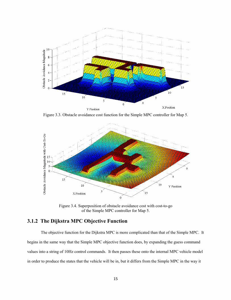
reactions to the obstacles. This creates a cost map that looks like that shown in Figure 3.3 for Map 5.

Once this obstacle avoidance cost has been tallied for the entire length of the solution trajectory, a final

cost-to-go, determined by the location of the final point of the solution, is added. This is meant to be an

estimation of the cost necessary to reach the goal from the end of the solution. In the simple MPC

implementation, this cost-to-go is simply calculated as the two dimensional distance to the goal from the

end of the trajectory. When this distance is superimposed with the obstacle cost, a map is produced that

provides some indication of the solution space that the Simple MPC controller is searching through, even

though it only evaluates the cost-to-go at the final point of the trajectory. This superposition is shown in

Figure 3.4 for Map 5.

15

Figure 3.3. Obstacle avoidance cost function for the Simple MPC controller for Map 5.

Figure 3.4. Superposition of obstacle avoidance cost with cost-to-go

of the Simple MPC controller for Map 5.

3.1.2 The Dijkstra MPC Objective Function

The objective function for the Dijkstra MPC is more complicated than that of the Simple MPC. It

begins in the same way that the Simple MPC objective function does, by expanding the guess command

values into a string of 10Hz control commands. It then passes these onto the internal MPC vehicle model

in order to produce the states that the vehicle will be in, but it differs from the Simple MPC in the way it

16

evaluates these states. This controller, instead of employing a varying obstacle avoidance cost, adds a

fixed cost whenever the vehicle trajectory passes within a given distance of the obstacle. These

avoidance regions are displayed in Figures 2.2 - 2.6. This fixed cost is set high enough that the optimizer

will continue to search commands until it finds a trajectory that doesn’t cross into the avoidance zone.

Therefore, the only real contribution to the command evaluation is represented by the cost-to-go value.

This is where the Dijkstra MPC gets its name. It employs Dijkstra’s algorithm [6] to find the shortest

path (composed only of line segments) from the end of the solution trajectory to the goal that doesn’t

cross into any of the avoidance regions. The Dijkstra cost-to-go function is plotted for Map 5 in Figure

3.5. It is easy to see that this function will discourage the vehicle from travelling towards a dead end,

unlike the one used by the Simple MPC. Here the optimizer will search for the control sequence that will

produce a path that will terminate with as low of a cost as possible. The topography of Figure 3.5 then

indicates that the solutions will be pulled effectively towards the goal.

Figure 3.5. Cost-to-go function used in Dijkstra MPC for map 5.

It was found that using the previously described Dijkstra objective function, the optimizer

occasionally output solutions that slowed around corners to an unnecessary extent. This was possibly due

17

to the discretized nature of the model in situations where the discrete points of the path fell just inside a

corner of the avoidance region. When this happened, the optimizer would adjust the velocity downwards

until a point would fall just outside the region. In order to encourage the optimizer to maintain high

speeds through the corners, an additional cost was added in the objective function to velocity control

values that were below the maximum control limit. This was found to effectively produce solutions that

maintained speed in the corners and were faster (overall) without crossing into the avoidance regions.

Another important parameter in the Dijkstra MPC configuration is the size of the avoidance

region around each of the obstacles. It was found that the optimal size for this parameter varies with

delay. For low delays, the vehicle follows the desired path more accurately, and a smaller avoidance

region allows for shorter paths that cut corners more tightly around obstacles. Therefore, as long as the

delay is low, no collisions will occur for small avoidance regions. However, when the delay is larger, the

vehicle travels farther from the expected trajectory and can sometimes travel through the entire avoidance

region and collide with an obstacle. These occurrences can be reduced by increasing the size of the

avoidance region, but as mentioned earlier, this produces longer paths. Another significant disadvantage

of larger avoidance regions happens if the region is expanded sufficiently so that avoidance regions of

neighboring obstacles overlap. In this case, it forces the vehicle to travel around both obstacles instead of

between them. For the purposes of the experiments in this thesis, a medium sized avoidance region was

chosen so that the Dijkstra MPC would not operate under the advantage of adjusting to different delays.

3.2 Potential Field Controller

The implementation of the Potential Field Controller, as mentioned above, adds artificial

repulsive forces to obstacles and an artificial attractive force to the goal. Specifically, the repulsive forces

are calculated using a fixed threshold distance, beyond which the obstacle has no affect, and the distance

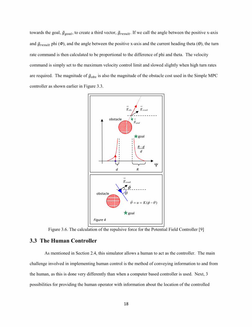
to the closest point on that obstacle. Figure 3.6 displays how this repulsive value is calculated. If R is the

threshold distance, and d is the distance to the closest point on the obstacle, a vector, ��, pointing away

from the obstacle is created with magnitude (R-d)/d. This vector is added to a unit vector pointing

18

towards the goal, ��, to create a third vector, ��. If we call the angle between the positive x-axis

and �� phi (Ф), and the angle between the positive x-axis and the current heading theta (Ѳ), the turn

rate command is then calculated to be proportional to the difference of phi and theta. The velocity

command is simply set to the maximum velocity control limit and slowed slightly when high turn rates

are required. The magnitude of �� is also the magnitude of the obstacle cost used in the Simple MPC

controller as shown earlier in Figure 3.3.

Figure 3.6. The calculation of the repulsive force for the Potential Field Controller [9]

3.3 The Human Controller

As mentioned in Section 2.4, this simulator allows a human to act as the controller. The main

challenge involved in implementing human control is the method of conveying information to and from

the human, as this is done very differently than when a computer based controller is used. Next, 3

possibilities for providing the human operator with information about the location of the controlled

φ

θ

( )u Kθ φ θ= = −&

R d Ψ

resultgur

goalgur

obsgur

resultgur

Figure 4

goal

obstacle

goal

obstacle

R - d

d

19

vehicle and its relationship to the obstacles and the goal are described. Each of these methods employs a

2-axis joystick as a means of acquiring the control signal from the human operator. As mentioned

previously, the joystick axes are scaled to produce u and v commands within the specified control limits.

The first method of providing the human with map information involves displaying an overhead

map view, just like in Figures 2.2 to 2.6, except rotated so that the goal lies at the top center of the screen

and the initial condition is at the bottom center. The vehicle is displayed in real time as a triangle or other

such directed shape. The problem with this is that it might be unnatural for some users to control a

vehicle that changes orientation on the screen. For example, if the vehicle gets turned around so that it

points toward the bottom of the screen, the human driver might think that pushing forward on the joystick

would cause the vehicle to move up on the screen, however, in this orientation, the vehicle would move

down. Similar difficulty can result when trying to turn the vehicle when it is oriented facing downwards.

These difficulties suggest another possible method of displaying the map information. That is,

show the vehicle in a fixed position, normally oriented upwards in the bottom center of the screen, and

move the map around according to the inverse of the command inputs. This way, when the driver turns

right, the obstacles always move left, and when the driver moves forwards, the obstacles always move

down, etc.

A third method, and possibly the most natural for a human, would be to display a first person

perspective type view in which the driver viewpoint is from the perspective of the vehicle looking out at

the obstacles in front of it. This view would naturally correspond to that seen by the driver of an actual

car. The only difficulty with this is that some distant objects could be obscured by closer ones, unless

some type of simulated transparency is used. A similar problem exists when trying to locate the goal. If

the goal is simply at eye level, the driver might not be able to see where it is much of the time. To

address this, one solution would be to place the goal above the obstacle height on some sort of pole, so

that even when an obstacle is between the driver and the goal, the driver would know where he/she should

be going.

20

3.4 Relating the Human Controller to the Autonomous Controllers

Because of the difference between the way the human and autonomous controllers use map

information, several methods of adjusting the information available to each controller have been devised

that attempt to mimic the amount of information that is available to each controller in various situations.

The basic method involves providing the entire map to the human just as described in Section 3.3.

This is most representative of the way the Dijkstra MPC functions, as it uses the location of all of the

obstacles to find the shortest straight line path to the goal around the obstacles. The information available

to the Simple MPC is limited to the length of the planned path, and therefore this path must be extended

in order to use the entire map. This can be done by allowing the optimizer to choose the control hold

times, indicated in Figure 3.1 as �t, and adding a constraint that the planned solution must end within a

specified distance to the goal. This would force the optimizer to solve for a feasible path that stretches the

entire way to the goal. However, with maps of several obstacles, the optimizers have significant

difficulty finding feasible paths. Even when they do, making even fine adjustments to the initial

command variables can force the solution to become infeasible. This difficulty severely limits the ability

of the optimizer to return even relatively sub-optimal solutions, and therefore this method was not further

developed. The Potential Field controller, by definition, only relies on extremely local information, and

therefore can’t be modified in any simply way to employ information from the entire map.

A second method of making the autonomous and human situations more comparable is to ignore

some of the information available. One such method involves masking obstacles that are farther than

some visibility threshold, rd. Figure 3.7 displays what the human view might look like in this case.

Naturally, this more closely corresponds to the way that the Simple MPC controller functions.

Additionally, the Dijkstra MPC controller could be modified to only use a limited range of information by

simply ignoring the obstacles outside of the sensing range when computing the shortest path to the goal.

21

Figure 3.7. Limited view for Human Controller [9]

The third possibility involves modifying the information available to the MPC controllers so that

they don’t possess an advantage over the human in the first person perspective arrangement. This can be

accomplished by either making the obstacles semi-transparent in the human view, or by ignoring the

portions of obstacles that are obscured by closer obstacles in the MPC map functions. This can again be

modified so that it mimics the Simple MPC information availability by using a limited sensing range.

Figure 3.8 displays the human view in this case. This final adjustment might be the most representative

of a vehicle entering an unknown environment in which it is only able to act on information gathered

from onboard sensors.

goal obstacle out of sensor range (will not be shown

to the driver)

dr

obstacle

vehicle

MAP

Driver’s View

22

Figure 3.8. Human First Person Perspective View and matching Overhead View [9]

goal

obstacle out of

sensor range

Figure 9

obstacle

First Person Perspective View

Overhead View

goal

obstacle out of

sensor range

obstacle

sensor range

vehicle

dr

23

CHAPTER 4

SIMULATIO RESULTS

This chapter is divided into Human results and autonomous controller results. These should not

necessarily be quantitatively compared due to differences in velocity and turn rate limits. Future work

will include performing experiments aimed at comparing the performance of humans and autonomous

controllers in exactly the same task.

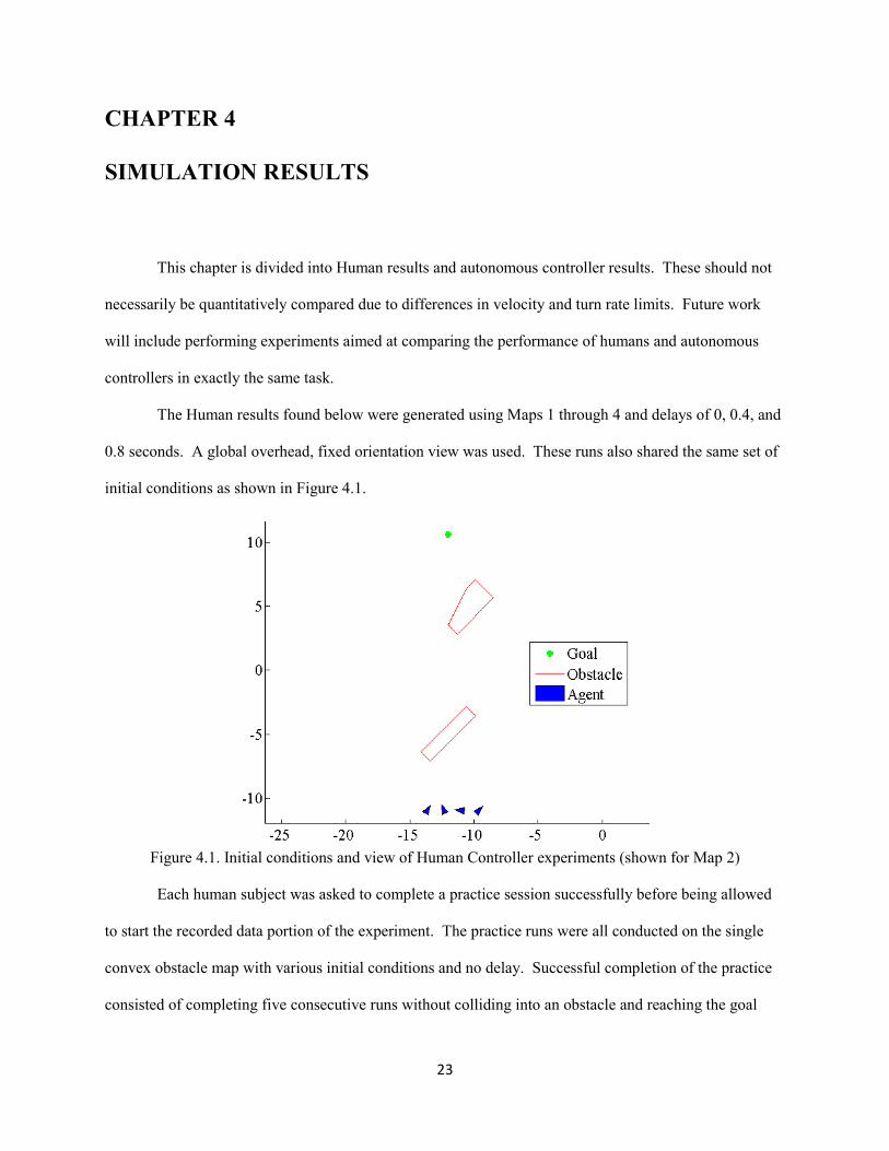
The Human results found below were generated using Maps 1 through 4 and delays of 0, 0.4, and

0.8 seconds. A global overhead, fixed orientation view was used. These runs also shared the same set of

initial conditions as shown in Figure 4.1.

Figure 4.1. Initial conditions and view of Human Controller experiments (shown for Map 2)

Each human subject was asked to complete a practice session successfully before being allowed

to start the recorded data portion of the experiment. The practice runs were all conducted on the single

convex obstacle map with various initial conditions and no delay. Successful completion of the practice

consisted of completing five consecutive runs without colliding into an obstacle and reaching the goal

24

region within 20 seconds. This process ensured that each subject was basically familiar with the controls

and had dealt with a significant portion of the learning curve prior to recording any data. For the recorded

session, each map, delay, and initial condition combination was repeated two times in randomized order.

The subjects were also shown the delay type. Either no delay, short delay, or long delay was displayed

corresponding to 0, 0.4, and 0.8 seconds. This prevented the humans from needing to waste time at the

beginning of each run figuring out which delay type was present. More research is being conducted to

examine the modes and performance characteristics of these human runs as well as taking many more

samples.

The results for the autonomous controllers in this thesis include only those from maps with

multiple obstacles as this accentuates the performance differences between the various controllers. Map 5

was also included in the autonomous experiment as a means of exemplifying the Dijkstra MPC

controller’s superior ability to avoid concave wells in more complicated and difficult situations.

4.1 Human Controller Results

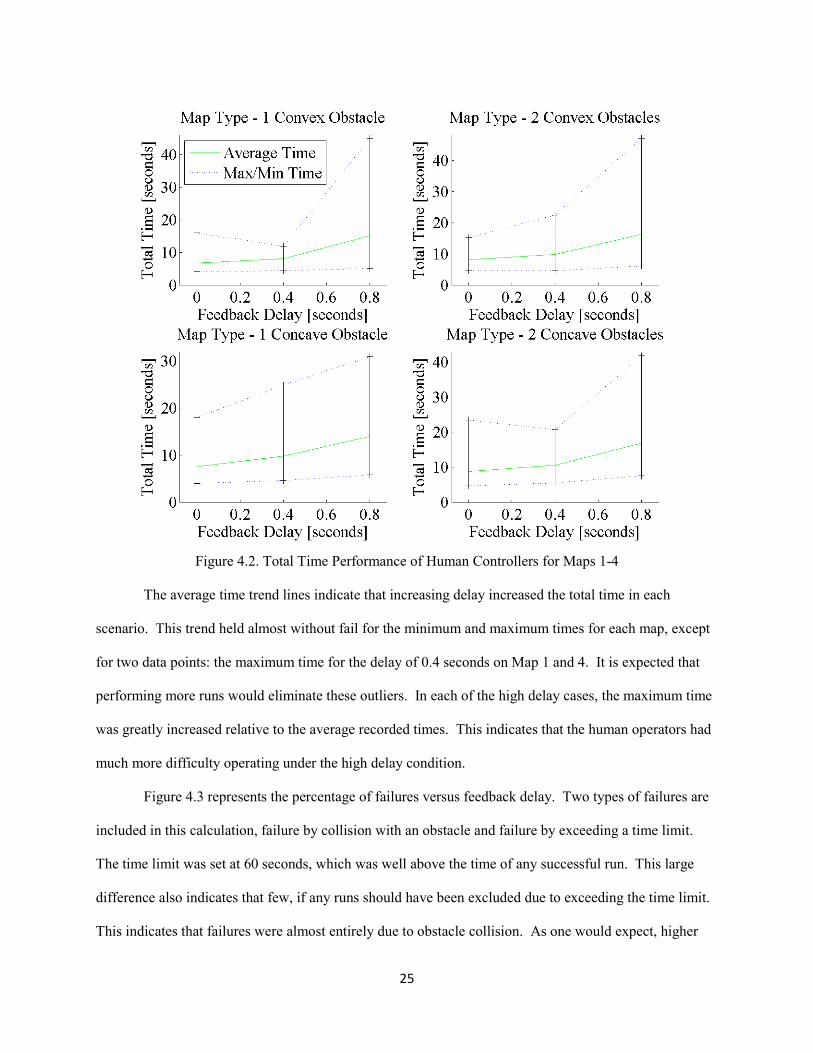
Figure 4.2 represents the performance of the human drivers with respect to time taken to reach the

goal. The horizontal axis in each of the four subplots represents feedback delay in seconds and the

vertical axis represents the total time in seconds. These graphs only take into account the experimental

runs in which the human drivers successfully reached the goal under the time limit and without colliding

into an obstacle. Each subplot displays three trend lines representing the minimum and maximum

successful times for each delay (the dotted lines), and the corresponding average times (solid green line).

The black vertical lines indicate the full range of recorded times.

25

Figure 4.2. Total Time Performance of Human Controllers for Maps 1-4

The average time trend lines indicate that increasing delay increased the total time in each

scenario. This trend held almost without fail for the minimum and maximum times for each map, except

for two data points: the maximum time for the delay of 0.4 seconds on Map 1 and 4. It is expected that

performing more runs would eliminate these outliers. In each of the high delay cases, the maximum time

was greatly increased relative to the average recorded times. This indicates that the human operators had

much more difficulty operating under the high delay condition.

Figure 4.3 represents the percentage of failures versus feedback delay. Two types of failures are

included in this calculation, failure by collision with an obstacle and failure by exceeding a time limit.

The time limit was set at 60 seconds, which was well above the time of any successful run. This large

difference also indicates that few, if any runs should have been excluded due to exceeding the time limit.

This indicates that failures were almost entirely due to obstacle collision. As one would expect, higher

26

delays increased the likelihood for failure. However, in each of the tested delays, the failure rate was

relatively low (as compared with the autonomous controllers discussed below), with a maximum of

around 13 percent. It is important to take these failure rates into consideration when examining the total

time figures because failed runs were not included in the total time calculations. This exclusion of failed

runs can provide a false advantage to the delays which experienced more failures because the worst runs

(those that did not finish) were not included in the total time performance. It is expected that the effect of

this advantage is small due to the low percentage of failures. Only one data point did not follow the trend

of increasing failure percentage with increasing delay: the 0.4 second delay on Map 3. It is expected that

if more data was collected, this outlier would disappear as well.

Figure 4.3. Percentage of Failures versus Feedback Delay for the Human Controller

Figures 4.4 through 4.7 show the actual paths taken in each experimental run. The obstacles are

outlined in red and the amount of delay is represented by the color of the path trace. The higher delay

27

cases, shown in blue, display a very large amount of unnecessarily tight turns. This shows how difficult it

was for the human operators to control the vehicle effectively. The higher delays sometimes led the

human operators to take on a go-stop-turn type strategy in which the operator would move forward

without turning for some distance, stop moving forward, turn incrementally until the desired orientation

was achieved and then repeat the process. If this strategy was not used, the paths often took on very

loopy and non-optimal shapes. It should be noted however, that even with these very random looking

trajectories, the percentage of failures was very low, indicating that when the vehicle was near an

obstacle, the humans tended to use more caution.

Figure 4.4. Human Controller paths for Map 1

28



29


4.2 Simple MPC, Dijkstra MPC, and Potential Field Controller Results

The results for the autonomous controllers are displayed in Figures 4.8 – 4.22 which are of three

types: total time versus delay, failure percentage versus delay, and actual path plots. The results shown in

these figures represent delays of 0, 0.2, 0.4, 0.8, and 1.6 seconds, maps with 2 convex, 2 concave, and 3

concave obstacles, and all three autonomous controllers (Simple and Dijkstra MPC, and Potential Field).

For each combination of the previously listed variables, 100 initial conditions were generated to have a

random position and orientation within the initial condition region shown in Figures 2.2 - 2.6.

Figures 4.8 – 4.10 display the percentage of failures on the vertical axis versus feedback delay on

the horizontal axis. Just like in the previously discussed human controller results, a failure is defined as

any run that didn’t reach the goal region within the allotted maximum time. Again, the maximum time

was set at 60 seconds but very few runs that were going to succeed failed due to the time limit. The vast

majority failed either because of a collision with an obstacle, or because they became trapped in a

potential well behind an object and circled there until the time limit was reached.

30

Several interesting trends can be seen here. Most notably, the Dijkstra MPC was the only

controller to successfully reach the goal on Map 5. However, the Dijkstra MPC displayed higher failure

rates than either the Simple MPC or the Potential Field controllers in the medium delays on map 2. This

could be explained by the fact that the Simple MPC and Potential Field controllers use avoidance

functions that extend farther from the obstacles than the Dijkstra MPC’s avoidance regions. The Dijkstra

MPC’s optimal path gets closer to the obstacle, and therefore, with higher delays, it is more likely to

wander into the obstacles than the other two controllers.

Figure 4.8. Percentage of Failures versus Feedback Delay for Map 2 for the autonomous controllers

31



32

Figures 4.11-4.13 display the total time to successfully reach the goal in seconds on the vertical

axis versus the feedback delay in seconds on the horizontal axis. Bars colored to indicate the controller

are placed in groups of three centered on each delay. Missing bars indicate that there were no successful

runs for that controller and delay pair. This can be seen in Figure 4.13 as there are only green bars

representing the Dijkstra MPC based controller. Each colored bar represents the average successful time

for that controller. Over each bar, there is a line that spans the range of successful runs, from the

maximum time to the minimum. For maps 2 and 4, it can be seen that the Dijkstra MPC controller

performed much better than either the Simple MPC or the Potential Field controllers. The minimum,

average, and maximum values for the Dijkstra MPC controller were at lower time values than the

respective values of both controllers at every delay on both maps.

It is important to notice that each average, minimum, and maximum value was calculated based

on different numbers of successful runs. The impact of this can be seen directly in Figure 4.13 as the

maximum total time trend for the Dijkstra MPC controller changes dramatically from 0.4 to 0.8 seconds

of delay. The maximum values are clearly increasing from 0 to 0.2 to 0.4, but then drop significantly for

a delay of 0.8 seconds. In examining the failure percentage graph for this particular map however, we see

that there is a significant increase in failure percentage from 0.4 to 0.8 seconds of delay. This means that

many of the possibly worst times were not counted because they were unsuccessful. This gives the 0.8

second delay maximum an artificial advantage and therefore any conclusions drawn from these trends

should take this into account.

33

Figure 4.11. Total Time versus Feedback Delay for map 2 for the autonomous controllers


34


Figures 4.14 - 4.22 display the path information from the individual runs for each of the tested

map and controller combinations. For each plot, the x and y axes represent the x and y position of the

vehicle. The amount of delay is indicated by the color of each trace. The region of initial conditions was

chosen so that multiple solution modes would be observed, i.e. some solutions would go around an

obstacle on the left and some on the right. A discussion of the effects of this on the data is provided in

Section 5.2.

35

Figure 4.14. Individual path traces for Map 2 for the Potential Field Controller

Figure 4.15. Individual path traces for Map 2 for the Simple MPC Controller

36

Figure 4.16. Individual path traces for Map 2 for the Dijkstra MPC Controller


37



38



39


In many of the runs the higher delay cases displayed varying degrees of oscillatory behavior.

This is the result of the delay between the observation of the current state, and when the command

appropriate for that state is implemented. For example, many times at the point that the state was

observed, it might be appropriate to turn left, and therefore the controller would produce a short plan of

sustained left turn. However, at the next observation point, the vehicle might have turned much too far to

the left, and therefore it would produce a plan to sustain a right turn, and the cycle would repeat. The

larger delay cases tended to show more and more exaggerated cyclical behavior which many times

resulted in collisions. Specifically this behavior can be witnessed in the Potential Field, 2 convex

obstacle case shown in Figure 4.14. In the space between the two obstacles where the zero delay case

essentially travelled straight towards the goal, the delayed controllers oscillated about this path in varying

amounts. The highest delay case, the yellow lines can be seen to bounce back and forth over the median

line to almost 2 meters on either side. The green line, representing 0.8 seconds of delay, bounces in a

similar fashion, but does so with a decreased magnitude.

40

The red traces in each plot represent the zero delay case and almost always represents the best

possible performance for each controller. In very few runs did any controller perform better under non-

zero delay.

The Dijkstra MPC paths, particularly those with low delays, follow very straight and seemingly

optimal trajectories. This is the result of the look-ahead ability of its cost-to-go function, as the Dijkstra

algorithm uses information about the entire map. The simple MPC cost-to-go function only uses the

straight line distance from the end of its solutions. Therefore when there is an obstacle between the

vehicle and the goal, but outside of its solution range, it will head directly towards the goal. Eventually

the (Simple MPC) vehicle’s solutions will come into contact with the avoidance region around the

obstacle and then it will start to detour around the obstacle. This happens only if the solution has enough

length to reach a point that produces a lower cost than points close to the vehicle. This can be seen in

Figure 4.21 in which the Simple MPC gets trapped behind the large center obstacle. Because the Simple

MPC solutions are limited in length, they cannot reach around the obstacle to find the lower cost points

on the other side. This is also the result of the gradient descent methods employed in the FMINCON

optimizer. In order to find the solution that would take the vehicle around to the opposite side of the

obstacle, FMINCON would need to incrementally send out predicted solutions that would first travel out

of the current potential well, eventually finding the negative gradient towards the goal on the other side of

the obstacle. Unfortunately, this is unlikely to happen because FMINCON would most likely stop

exploring that area of the solution space because it would find that going in that direction at first would

seem more costly.

41

CHAPTER 5

COCLUSIOS, OTHER OTES, AD FUTURE WORK

5.1 Summary and Conclusions

The software described in this document represents a stable and useful tool for analyzing the

performance of various controllers performing obstacle avoidance tasks with delay.

Several autonomous controllers as well as humans acting as controllers were tasked with

navigating an obstacle field towards a goal in minimum time and the results were analyzed.

The autonomous controllers consisted of a simple artificial potential field controller as well as

two implementations of Model Predictive Control. The MPC based controllers differed mainly in the

cost-to-go function that they employed. One used a simple 2-dimensional distance and the other used the

Dijkstra Algorithm to find the shortest path through a network of connected nodes.

The MPC controller which used the Dijkstra Algorithm performed significantly better on average

than either of the two autonomous controllers. Its implementation allowed it to avoid artificial potential

wells and to always choose the shortest path towards the goal.

5.2 Other otes and Concerns

It should be taken into consideration that the experiments described within this thesis represent an

incredibly small portion of those setups allowed by the simulator.

Many decisions were made when designing the maps and various parameters that were based on

nothing more than the hope that it would lead to interesting results. Many combinations were attempted

that led to very poor performance by the autonomous controllers, or were much too easy for their human

counterparts. It should be noted therefore that these results in no way represent an exhaustive set, but

instead are only a representative example of the configurations that are available.

42

The dependability of the solutions produced by the FMINCON and PATTERNSEARCH

optimizers in MATLAB is also not complete. The solution space that these optimizers were searching

through is of high dimension and complexity. This leads to the existence of many local minimum which,

to the casual observer, would appear to be totally non-optimal. Therefore much tuning and adjusting of

parameters and even addition and subtraction of terms was necessary in order to produce the quality of

the solutions found in this document. This necessary amount of tuning should be taken into consideration

if one wants to apply any of these controllers to other situations.

5.3 Future Work

One possibility is to obtain simulation results for the exact maps and initial conditions that the

human experiments used so that meaningful comparisons can be made between human and autonomous

controller performance. This task involves more than simply initiating the same simulations with

different bounds as the individual controllers and optimizers perform differently under different

magnitudes of inputs. These controllers would each need to be tuned to these much faster speed limits.

Another interesting task would be to divide the simulator solutions into their modes of task

completion and analyze each mode independently, i.e. group all of the solutions together that reach the

goal by going around the first obstacle on the left instead of the right. This could provide more reliable

trends in the total time and failure percentage as some modes might cause many more collisions, yet reach

the goal in less time.

It would also be possible to obtain human subject data and autonomous controller data for maps

that require much more accurate and slow maneuvering around complicated obstacles. This might lead to

higher failure rates as both the human and autonomous controllers would encounter difficulty with the

higher delays when close to obstacles.

Finally, it would be possible to obtain human subject data that corresponds to each of the

described cases of limited visibility, occlusion, and global visibility. Then one could analyze these results

and compare them to the performance of the autonomous counterparts.

43

BIBLIOGRAPHY [1] Qin S.J., and Badgwell, T.A. “A survey of industrial model predictive control technology,” Control

Engineering Practice, vol. 11, no. 7: pp. 733–764, 2003. [2] Findeisen, R., and Allgöwer, F. “An introduction to nonlinear model predictive control,” in In

Proceedings 21st Benelux Meeting on Systems and Control, Veldhoven, 2002. [3] Camacho, E., and Bordons, C. Model Predictive Control. London, UK: Springer, 1999. [4] Nicolao, G.D., Magni, L., and Scattolini, R. “Stability and robustness of nonlinear receding horizon

control,” in onlinear Model predictive control, F. Allgöwer and A. Zheng, Eds. Birkhäuser Verlag, Basel, Switzerland, vol. 26, 2000.

[5] Know, W., and Han, S. “Receding Horizon Control: model predictive control for state models,” in

Advanced Textbooks in Control and Signal Processing, 1st ed. London: Springer, 2005. [6] Dijkstra, E. W. "A note on two problems in connexion with graphs," umerische Mathematik, vol. 1:

pp.269–271, 1959. [7] Bellingham, J., Richards, A., and How, J.P. "Receding horizon control of autonomous aerial vehicles,"

in Proceedings of the 2002 American Control Conference (IEEE Cat o CH37301) ACC-02, 2002. [8] “About The MathWorks,” The MathWorks Homepage, Web, Apr. 2010. [9] Burns, C., Zearing, J., Wang, F.R., and Stipanović, D.M. “Autonomous and Semiautonomous Control

Simulator,” in Proceedings of The 2010 AAAI Spring Symposium on Embedded Reasoning, Mar. 2010.

[10] Đnalhan, G., Stipanović, D.M., and Tomlin, C.J. “Decentralized Optimization with Application to

Multiple Aircraft Coordination,” in Proceedings of the 2002 IEEE Conference on Descision and

Control, pp. 1147-1155, Dec. 2002. [11] Mejía, J.S., and Stipanović, D.M. “Safe Coordination Control Policy for Multiple Input Constrained

Nonholonomic Vehicles,” in Proceeding of the Joint 48th IEEE Conference on Decision and Control

and 28th Chinese Control Conference, Shanghai, P.R. China, pp. 5679:5684, Dec. 2009. [12] Saska, M., Mejía, J.S., Stipanović, D.M., and Schilling, K. "Control and navigation of formations of

car-like robots on a receding horizon," in Proceedings of the 2009 IEEE International Conference on

Control Applications, pp.1761:1766, 2009. [13] Khatib, O. “Real-Time Obstacle Avoidance for Manipulators and Mobile Robots,” in The

International Journal of Robotics Research, vol. 5: pp.90:98, Mar. 1986.

a simulator for autonomous and semiautonomous by …

Documents