A Skeptical View of the Impact of the Fed’s Balance Sheet

David Greenlaw Morgan Stanley

James D. Hamilton

University of California at San Diego and NBER

Ethan S. Harris Bank of America Merrill Lynch

Kenneth D. West

University of Wisconsin and NBER

May 2018

We thank Aditya Bhave, Molly Wharton and Anna Zhou for excellent research assistance. We benefited from comments on earlier drafts of this paper by our discussants William Dudley and Eric Rosengren, and by Stephen Cecchetti, Jason Cummins, Mike Feroli, Jan Hatzius, Peter Hooper, Anil Kashyap, Rick Mishkin, Glen Rudebusch, Brian Sack, Kim Schoenholtz, Eric Swanson, Amir Sufi, and Xu Zhang.

ABSTRACT/EXECUTIVE SUMMARY

We review the recent U.S. monetary policy experience with large scale asset purchases (LSAPs) and draw lessons for monetary policy going forward. Most previous studies have found that quantitative easing (QE) lowered long term yields, with a rough consensus that LSAP purchases reduced yields on 10-year Treasuries by about 100 basis points. We argue that the consensus overstates the effect of LSAPs on 10-year yields. We use a larger than usual population of possible events and exploit interpretations provided by the business press. We find that Fed actions and announcements were not a dominant determinant of 10-year yields and that whatever the initial impact of some Fed actions or announcements, the effects tended not to persist. In addition, although the Fed began the transition to a smaller balance sheet sooner than the market had expected, the announcements and implementation of the balance-sheet reduction do not seem to have affected rates much. These observations lead us to conclude that the effects of LSAP are likely more modest than generally claimed. Going forward, we expect the Federal Reserve’s balance sheet to stay large. This calls for careful consideration of the maturity distribution of assets on the Fed’s balance sheet. Our conclusion is that the most important and reliable instrument of monetary policy is the short term interest rate, and we discuss the implications of this finding for Fed policy going forward.

1  

In this paper we review the recent U.S. monetary policy experience with large scale asset

purchases and use our review to draw lessons for monetary policy going forward.

In response to the financial crisis and the Great Recession, the Federal Reserve instituted

a series of rate cuts that lowered the overnight rate effectively to zero in December 2008. With a

perceived need for further loosening, and with the overnight rate stuck at the zero lower bound,

the Federal Reserve turned to unconventional policy. One of its major unconventional tools

involved large scale asset purchases (LSAPs) of long term Treasuries and other securities. A

voluminous literature has found that such purchases affected long term yields. Perhaps a

consensus figure is that the programs lowered the 10 year Treasury yield by about 100 basis

points (for example, see Borio and Zabai (2016)).

The Federal Reserve has recently begun to scale down the size of its balance sheet. This

raises the question of whether downsizing will have effects comparable in magnitude, but

opposite in sign, to the effects associated with expansion of the balance sheet. And quite apart

from transitional effects, there is the issue of whether LSAPs should play a regular role as a

monetary policy tool.

Recent reviews of the impact of LSAP programs include Borio and Zabai (2016),

Dell’Ariccia et al. (2017) and Kuttner (2017). We build on these studies by providing new

evidence on the overall importance of LSAPs in driving real and nominal 10-year bond yields.

Our paper is organized roughly chronologically. Sections 2 and 3 review the theory of

conventional and unconventional monetary policy. Sections 4 and 5 present new evidence on the

U.S. experience with QE programs, with Section 4 focusing on expansion of the balance sheet

and Section 5 on the period from the first hints of tapering to the initial stage of unwind. Section

2  

6 considers the future evolution of the balance sheet, both empirically and theoretically, as well

as some linkages to fiscal decisions. Section 7 makes policy recommendations.

In more detail:

We begin our paper (Section 2) by reviewing how monetary policy worked before the

financial crisis. Our view is similar to the standard textbook version–raising or lowering the

overnight rate leads to changes in long term yields, including real private borrowing rates. We

also note that considerable econometric evidence indicates that such adjustments in the overnight

rate have persistent effects on long rates.

Section 3 reviews the theory of unconventional monetary policy. In our view, negative

interest rates have limited potential. And forward guidance, which is powerful in theory, is not

easy to implement effectively in practice. Forward guidance aside, large scale asset purchases

(LSAPs) can work through a portfolio balance channel. This channel is ruled out in many

standard economic models, but could arise under some formulations of preferred habitat or other

market imperfections. How effective LSAPs might be in practice is very much an empirical

question. The cross-country and historical evidence suggests that the monetary authority is able

to influence long rates through LSAPs. The relative contribution of forward guidance versus

portfolio balance is unclear, as is the magnitude of the effect.

Section 4 takes a closer look at the effectiveness of the Fed’s LSAP programs. We note

that we are not commenting here on the potential effectiveness of the emergency loans that the

Fed initiated in September and October of 2008, but begin our analysis with the large-scale

purchases of Treasury and mortgage-backed securities that came later. In event studies such as

Gagnon et al. (2011) and Krishnamurthy and Vissing-Jorgensen (2011), the researcher studies a

3  

handful of key dates where the Fed clearly moved the markets. We argue that this is useful for

finding “clean” experiments, but is less useful for gauging the sustained, full impact of LSAPs.

We instead adopt two more comprehensive approaches. First, we examine changes in

yields on “Fed News Days”—all days of FOMC announcements, release of minutes and policy-

related speeches by the Fed Chair. The sum of these should capture the general impact of the

Fed over time, along with some noise for days on which the Fed didn’t matter much. Second, we

look at any day on which there is a one-standard deviation change in bond yields, and use the

Reuters bond market wrap up to label the cause of the bond market move that day. We use

“Reuters Fed News” as a label for a day in which bond yields change by one standard deviation

and Reuters attributes the change in part to news about Federal Reserve statements or actions.

We use labels such as “macro data” and “Europe news” for Reuters attributions on other one

standard deviation days. We focus on days where there was at least a one standard deviation

change in bond yields on the assumption that it is easier for Reuters to identify the cause of

market moves when the move is large.

Skeptics of QE point out that yields generally rose during the implementation of each

round of QE—QE1, QE2 and QE3. Consistent with that finding, our analysis produces smaller

policy impacts than in event studies focusing on big announcements. In particular, we find that

yields tend to rise on “Fed Days” and “Reuters Fed News” days that are subsequent to the big

surprise days. We do not attempt to establish why this is the case. One possibility is that market

participants eventually decided that the initial response represented an overreaction, or they had

anticipated a subsequent flow of announcements that never materialized. Another is that some

responses in non-Fed days were so strongly colored by market views of Fed policy that, despite

the Reuters attribution, those responses should be properly be counted in part as a “Reuter Fed

4  

News” day. A third possible factor, as noted in Hamilton and Wu (2012) and Greenwood,

Hanson, Rudolph, and Summers (2016), is that the Treasury unexpectedly undercut the Fed’s

programs, thereby muting any possible portfolio balance effect. We note that our finding is

consistent with studies such as Swanson (2017) that find that the effects of forward guidance die

out very quickly.

Section 5 begins our discussion of the exit from unconventional policy by analyzing

events from the first talk of tapering through the early stages of balance sheet normalization in

2017. Our procedure attributes most of the bond market sell-off during the 2013 “taper tantrum”

to better economic news rather than to changing expectations for the end of balance sheet

expansion. And even when plans for exit were gelling, a comparison of January 2017 survey

answers with actual outcomes reveals that the Fed was more hawkish than market participants

expected (for example, starting shrinkage sooner than expected). Nonetheless, there did not

seem to be much of a market reaction – a phenomenon we describe as the “shrinkage shrug.”

Consistent with the conclusions from Section 4, the implication would seem to be that

movements in the balance sheet, and surprise decisions about the balance sheet, have modest and

uncertain effects on yields.

Section 6 looks ahead at the evolution of the balance sheet. Because of normal growth in

the economy and changes in operating procedures, we expect the balance sheet to start to expand

again after a few years, even if the Fed follows its planned unwind over the nearer term. Some

Federal Reserve documents (for example, Federal Reserve Bank of New York, 2017) present a

scenario in which the average reserve balance ends up around $100B. We think this is

unrealistic absent a significant change in the Fed’s current operating procedures. Among other

5  

factors, Treasury balances and reverse repurchase agreements are so large and volatile that

offsetting them with small reserve balances could produce big spikes in interest rates.

On a related but distinct topic, Section 6 also considers policy aspects of the duration of

assets on the balance sheet. We endorse recent Treasury moves to make its decisions about the

weighted average maturity of the debt more predictable and model driven. This would allow the

Fed to be last mover, making it less likely that Fed and Treasury actions will work at cross

purposes when the Fed is adjusting its balance sheet. We also note some of the tradeoffs

involved in the Fed’s decisions about duration.

Section 7 makes policy recommendations. The starting point is our view that LSAPs

have uncertain effects. The most important and reliable instrument is control of the short term

interest rate. In terms of the balance sheet, we recommend a “Treasuries first” policy, with the

Fed perhaps holding a small amount of MBS to signal that purchases of MBS are not completely

out of the question. The Fed should mostly hold short term Treasury securities. Finally, in terms

of the ongoing unwind, the Fed should consider larger and looser caps on the amount of

redemptions.

Our overall conclusion is that the size of the Fed’s balance sheet is less potent in moving

the bond market than as perceived by many and should not be viewed as a primary tool of

monetary policy going forward.

2. Monetary policy goes from conventional to unconventional

Let us begin with an overview of conventional monetary policy transmission, as practiced

in the pre-crisis period. Suppose the monetary authority—from now on, the Fed—wishes to

stimulate the economy. Then it lowers the target rate for federal funds rate. When the target rate

6  

falls, in general, so, too, does the whole spectrum of interest rates, on private as well as public

loans, and on loans of all maturities. This, in turn, triggers a general easing of financial

conditions. Because prices and expected inflation are sticky, this fall in nominal rates also lowers

real rates. This stimulates interest-sensitive private sector expenditures such as home

construction..

Needless to say, the lags from interest rate adjustment to economy-wide response are

long and variable. The transmission mechanism to the macroeonomy is not within the scope of

our paper, however, and we henceforth abstract from such transmission and focus on movements

of long term interest rates in response to monetary policy decisions.

A number of studies have concluded that Fed actions had significant effects on long-term

yields during the pre-2008 period (see among others Cook and Hahn, 1989 and Kuttner, 2001).

These papers find that yields on Treasuries of all maturities move in the same direction as that of

the target rate, with the effect monotonically declining with horizon. There is variation in the

response in different decades. But, to oversimplify, these papers indicate that a 100 basis point

surprise cut in the target rate results on impact, in roughly a 50‐75 basis point decline in

Treasuries with less than one year to maturity. The impact effect diminishes with maturity, with

20 or 30 year Treasury yields falling by roughly 10-20 basis points.

The previous paragraph inserted the word “surprise” before “cut.” The empirical

literature finds a difference between expected and surprise components of changes in target rates.

This is consistent with models of the term structure of interest rates. Long term rates are the sum

of two components, the average of expected future short term rates, and a term premium.

Changes in an overnight rate such as the federal funds rate can potentially affect the path of both

components. But to the extent that the change in the target rate is anticipated, the actual

7  

adjustment of the interest rate will cause little to no adjustment of the path of expected future

rates and hence have a diminished impact: market participants will incorporate anticipation of

the Fed’s future target for the short rate into the pricing of current long-term yields. Changes in

current or expected future short-term rates could affect market risk premia. An example of an

empirical study that concludes that adjustments in short rates affect both expected future short

rates and term premia is Hanson and Stein (2015).

This conventional view overlooks forward guidance that stands apart from an interest rate

adjustment, a distinction we do make in our discussion of unconventional policy below. It also

abstracts from a possible direct effect of Fed words or actions on bank balance sheets or on asset

prices other than bonds. Nonetheless, we take our description to capture a central element of

how monetary policy affects the economy in periods such as the pre-crisis era.

As an empirical matter, surprise adjustments of short rates importantly affected both

shorter and longer rates not only on impact but persistently. The fact that movements in short

rates are persistent is stylized fact in macroeconomics, often captured with a lagged interest term

in a monetary policy rule. In term of longer rates, research includes Bernanke, Boivin and Eliasz

(2005) and Gertler and Karadi (2015), who find 5 and 10 year yields still responding to monetary

policy shocks one to two years after the shock (with mixed statistical significance).1 As well,

Bekaert, Cho and Moreno (2010) find that term structure variables respond persistently and

significantly to monetary policy shocks for roughly a year, with monetary policy the dominant

determinant of term structure factors. We shall suggest below that in the era of unconventional

                                                            1 Gertler and Karadi’s baseline results are for a sample that runs to 2012. Their robustness results indicate the cited result applies to a sample that ends in 2008. Ramey argues that in studies such as these magnitudes and even signs of responses may not be robust. However, inspection of her graphs indicates that persistence of response is a robust feature.  

8  

policy, it is not obvious that monetary policy decisions had a persistent and dominant effect on

long rates.

For the transition from the pre-crisis era to the present, Exhibit 2.1 lists some key

programs and events. The cut in interest rates in September 2007 was probably viewed by most

as the usual beginning of an easing cycle. But the financial crisis brought forth a vigorous

response that went well beyond interest rate cuts. The now-defunct programs such as those listed

in line (2) of Exhibit 2.1 were intended to stabilize the financial system rather than provide the

sort of stimulus that comes from lowering interest rates, and we shall not have occasion to say

anything more about these programs.

Once the zero lower bound was reached in December 2008, lowering rates could not be

accomplished by lowering the federal funds target. So various programs, labeled in Exhibit 2.1 -

-as QE1, QE2, the maturity extension program, and QE3 were introduced.2 Such programs

aimed to start the process of lowering the whole yield curve3 by targeting rates on long maturity

bonds. The logic is described in the next section. In terms of mechanics, those programs

involved announcements and actions to purchase certain long maturity bonds.

Exhibit 2.2 displays the assets of the Federal Reserve since the end of 2002. These

quintupled between 2007 and 2014 and stood at $4.5 trillion at the beginning of 2018. This

balance-sheet expansion came in two distinct phases. The first came in the Fall of 2008 in the

form of a variety of programs to provide emergency loans including Term Auction Credit, the

Commercial Paper Funding Facility, and currency swaps. These are indicated by dark purple in

Exhibit 2.2. As noted above, our paper does not address the potential efficacy of this first phase

                                                            2 As discussed in the next section, precedents for these programs include “Operation Twist” in the U.S. (Swanson (2011)) and various programs in Japan (Michaelis and Watzka (2017)). 3 And, in the case of MBS purchases, to specifically help the housing market. 

9  

of using the Fed’s balance sheet. Our analysis instead focuses on the later expansion of Fed

holdings of Treasury bonds (shown in pink) and mortgage-backed securities (MBS, in turquoise)

purchased in QE1, QE2, and QE3. The pink and turquoise regions measure the par value of

these securities. On average, the Fed paid a price slightly above par in acquiring these. The Fed

does not report a breakdown of the premium on Treasuries versus MBS, so Exhibit 2.2 follows

the convention of the H.4.1 release in treating unamortized premia net of discounts as a separate

asset.

Exhibit 2.3 shows how these assets were financed in terms of the liability side of the

Fed's balance sheet. Note that by definition, the cumulative height in Exhibit 2.3 is identical to

Exhibit 2.2. Of the $4.5 T in assets at the start of 2018, about half were financed by deposits of

financial institutions held at the Fed (purple), a little more than a third by currency in circulation

(green), and most of the rest from the Treasury's Fed balance (in yellow) and reverse repos

(orange). The latter can be thought of as collateralized loans to the Fed primarily coming from

money market funds

 

3. The impact of unconventional policy

3.a. How unconventional policy works in theory

As noted in the previous section, traditional monetary policy operates through control of

short-term interest rates. But the fed funds rate was brought essentially to zero by the end of

2008. There are three options available to the central bank to try to provide additional stimulus

in such a situation. First, the central bank can try to push nominal interest rates into negative

territory. Second, the central bank can use forward guidance to try to communicate its intended

future path for the policy rate. Third, the central bank can purchase other assets (or “twist” its

10  

asset holdings) to try to influence long-term interest rates or the exchange rate. Asset purchases

can be further broken down in terms of the kinds of assets bought and the operating procedures

within which the purchases are implemented. We now discuss each of these options in turn.

3.a.1. Negative interest rates.

The Federal Reserve has paid a modest positive interest rate on excess reserves since the

fall of 2008. But the ECB and central banks of Sweden, Switzerland, Denmark, and Japan ended

up imposing fees on some deposits held at the central bank, which can be viewed as a negative

interest rate on those deposits. If a bank lends its central bank deposits to another bank

overnight, it could avoid the fee, though this just passes the deposits to another bank. Banks are

willing to pay another bank to take the deposits off their hands, and in equilibrium, the interest

rate on interbank loans, like the interest rate on deposits held at the central bank, will be bid into

negative territory.

An individual bank could also avoid the fee by purchasing a government security from

another bank, sending its deposits to the other bank. Again, aggregate deposits with the central

bank do not disappear as a result of such transactions. But the result will likely be that the

interest rate on government debt becomes negative as well.

Exhibit 3.1 updates the analysis of Alsterlind et al. (2015) of the experience in Sweden.

The Riksbank lowered its policy repo rate to 0.25% in March 2015 and had brought it down to

0.50% by February of 2016. The interest rates on 3-month loans between banks and 2-year

government debt quickly became negative as well, and even the 2-year mortgage rate was

negative by June of 2016. By driving the policy interest rate negative, the central bank thus has a

tool with which it could encourage additional borrowing and spending.

11  

Another way banks could avoid the fees is by withdrawing their deposits with the central

bank in the form of cash. Hoarding cash is sufficiently costly and inconvenient that it has not

been a major factor in the countries experimenting with negative rates, though it could become

more important if the central bank tried to drive the interest rate deeper into negative territory.

Moreover, retail customers might hoard cash to avoid even modest charges. This may be one

reason that many banks have been reluctant to fully pass the charges along to customers, as seen

in Exhibit 3.2. Studies by Heider, Saidi, and Schepens (2016) in the Euro Area and Eggertsson,

Juelsrud, and Wold (2017) in Sweden found distinctly less pass-through of the policy rate into

aggregate lending rates once the policy rate became negative.

To the extent that the negative rates are not fully passed through to customers, the policy

amounts to a tax that decapitalizes banks at a time when maintaining the health and stability of

financial institutions may be a key policy goal. Heider, Saidi, and Schepens (2016) and

Eggertsson, Juelsrud, and Wold (2017) found that the more important customer deposits were as

a source of bank funding, the slower the growth in lending from the bank once interest rates

become negative. Eggertsson, Juelsrud, and Wold (2017) noted that as a result of this effect, the

net consequences of negative interest rates on aggregate spending could actually be

contractionary, a possibility also demonstrated by Brunnermeier and Koby (2016).

The net stimulatory potential of bringing the policy rate from 0 down to 0.50% thus is

likely not very large, and it’s probably not possible to go much below this without encouraging

more widespread unproductive hoarding of cash. Some authors, including Goodfriend (2016)

and Rogoff (2016) noted that additional measures could be considered to utilize negative rates

more aggressively, such as banning large-denominational currency to further raise the cost of

12  

hoarding cash. In the absence of such institutional changes, the potential stimulus from negative

interest rates seems very limited.

3.a.2. Forward guidance.

When the federal funds rate reached its effective lower bound, everyone expected that

one day the U.S. would eventually return to a regime of positive interest rates. If the Fed can

effectively promise to keep rates low for a longer period, this could potentially be a source of

stimulus even while interest rates are still at the lower bound. For example, anticipation of

higher inflation in 2016 could in principle influence the spending decisions of consumers and

firms in 2009. In many economic models, if one takes the anticipation of policy in the distant

future as something that can be arbitrarily changed, adjusting those expectations turns out to be a

powerful tool for stimulating the economy at the zero lower bound (ZLB). Indeed, this tool is

predicted by theory to be so powerful that some researchers have developed doubts about the

theoretical models themselves; see for example Del Negro, Giannoni and Patterson (2012) and

McKay, Nakamura and Steinsson (2016).

The Fed made its first stab at forward guidance at the August 9, 2011 FOMC meeting,

issuing the following statement:

“The Committee currently anticipates that economic conditions–including low rates of

resource utilization and a subdued outlook for inflation over the medium run–are likely to

warrant exceptionally low levels for the federal funds rate at least through mid-2013.”

Swanson and Williams (2014) noted that in the month prior to this FOMC statement, the Blue

Chip consensus was that the fed funds rate would not be raised until 3 more quarters. After the

statement, the estimate jumped to 7 or more quarters (see Exhibit 3.3), demonstrating that the

Fed indeed has the power to influence market expectations with statements like this one.

13  

But what exactly was the Fed communicating? Campbell et al. (2012) noted two

possibilities, both inspired by stories from Greek mythology. In “Odyssean forward guidance,”

the Fed with announcements like this is committing itself to a future course of action, like

Odysseus bound to the mast of his ship, even though the Fed might later wish it could make a

different choice. By contrast, in “Delphic forward guidance,” the Fed, like the Oracle of Delphi,

is simply communicating information it has that the market does not. Such information could

either be about the Fed’s own preferences—you may not know it, but we’re really doves at heart,

and that’s why we’re not about to raise interest rates—or about the Fed’s superior knowledge of

the state of the economy—the economy is in much worse shape than you think, and that’s why

we’re not about to raise rates. The former would presumably serve as an expansionary Delphic

signal, whereas the latter could lead to further pessimism and actually make the situation worse.

Empirical analysis by Campbell et al. (2012) and Nakamura and Steinsson (forthcoming)

concluded that the second Delphic channel, operating through the Fed’s superior information

about weak fundamentals, accounts for a significant component of the market’s reaction to

Federal Reserve communication of its future intentions. Bhattarai, Eggertsson and Gafarov

(2015) presented an alternative model in which LSAP is effective because it generates a credible

signal of low future real interest rates in a time-consistent equilibrium.

3.a.3. Large scale asset purchases.

The other main policy tool that the Fed relied on during the period of exceptionally low

interest rates between 2009 and 2014 was open-market purchases of securities in very large

volume. In contrast to the potentially strong role for forward guidance in many macroeconomic

models, large-scale asset purchases (LSAP) for an economy at the zero lower bound would have

no effect on inflation, nominal interest rates, or any real variable in most standard models. The

14  

reason is that if the public’s demand for high-powered money is already saturated, purchasing

any asset with newly created Federal Reserve deposits does not change the pricing kernel that

determines any asset price or private spending decision (see for example Eggertsson and

Woodford, 2003). As Ben Bernanke put it just before he stepped down as Chair of the Federal

Reserve, “the problem with QE is it works in practice, but it doesn’t work in theory.”4 Here we

consider different possible channels whereby the purchases might have an effect by

distinguishing between the kind of securities purchased and the way the program is implemented.

Large-scale purchases of Treasury Securities. A Federal Reserve purchase of a long-

term Treasury security essentially swaps one liability of the U.S. government (for example, a 10-

year Treasury note) for a very short-term liability (interest-bearing overnight deposits with the

Federal Reserve). While a Modigliani-Miller Theorem (for example, Wallace, 1981) might

suggest that the maturity composition of outstanding government debt does not have any real

effects, in practice the Treasury pays a premium when it issues long-term debt instead of short,

apparently willingly compensating bond holders for absorbing a state-contingent risk that the

Treasury or the Fed would otherwise have to bear. For example, if a higher fraction of publicly

held Treasury debt is of short duration, in some states of the world the Treasury might be forced

to raise distortionary taxes or the Fed tolerate higher inflation in a situation where they would

prefer not to be forced to do so. Hamilton and Wu (2012) and Eggertsson and Proulx (2016)

proposed this as one possible mechanism whereby LSAP could end up exerting real effects,

essentially as a form of Odyssean state-dependent forward guidance which could potentially

influence long-term interest rates through both an expectations component and the term

premium.

                                                            4 See https://www.ft.com/content/3b164d2e-4f03-11e4-9c88-00144feab7de. 

15  

Woodford (2012) noted that Fed purchases of Treasury securities could also have real

effects by influencing a possible safety premium. Financial institutions use certain safe assets

like Treasury securities as collateral in repo transactions, which gives these securities value

beyond that associated with their state-contingent pecuniary returns alone. Central-bank

purchases or sales of long-term Treasury securities might be able to affect the size of the safety

premium, and thus affect long-term yields even in the absence of any change in the expected

path of short rates. The theoretical model in Caballero and Farhi (2017) provided one way to

represent such effects.

More generally, LSAP could have real effects whenever some investors have preferences

for bonds of certain maturities or are limited in the set of securities they are willing to buy. If

this is the case, a decrease in the supply of a particular security (for example, if the Fed buys up a

significant fraction of outstanding long-term Treasury bonds) would increase the price of those

securities and depress the yield on those bonds relative to others. This channel is typically

described as a “portfolio balance effect,” an extreme version of which assumes that certain

institutions are completely unable to hold certain securities. Theoretical models incorporating

versions of this idea include Chen, Curdia and Ferrero (2012), and Greenwood and Vayanos

(2014).

Large-scale purchases of other securities. In addition to purchasing Treasury securities,

the Federal Reserve also bought large quantities of mortgage-backed securities, a strategy

sometimes referred to as “targeted asset purchases” or “credit easing.” Again this would have no

impact on mortgage rates in models like Eggertsson and Woodford (2003), but portfolio-balance

effects could allow these purchases to affect yields as in Curdia and Woodford (2011) and

16  

Gertler and Karadi (2011). Some of the empirical evidence surveyed below suggests that

purchases of MBS had a stimulatory effect over and above that of the Treasury purchases.

Using LSAP to target exchange rates or interest rates. Large-scale asset purchases could

in principle be specified in terms of quantities (buy so many billions of long-term Treasuries, for

example) or in terms of fixed price targets (keep on buying until the 10-year yield reaches a

specified target). Again, unless the central bank can somehow commit to a particular policy rule

once the economy escapes from the zero lower bound, no volume of purchases could achieve a

specified target for the 10-year yield under the assumptions in Eggertsson and Woodford (2003).

In September 2017, the Bank of Japan adopted a version of this in the form of yield curve

targeting, announcing its intention to purchase Japanese government bonds (JGB) so that the 10-

year JGB yield would remain at around zero percent. One could argue that the policy so far has

been successful. The 10-year JGB yield has remained around 7 basis points since the Bank’s

announcement, a period when 10-year German yields rose 20 bp and 10-year U.S. Treasuries

rose by 50 bp. However, it may be that yield curve control only works if interest rates and

inflation expectations are already low. Yield curve control came after years of low interest rates

and deflation, making it easier to maintain the peg.

The Swiss National Bank tried to commit to a target exchange rate, but gave up in

January 2015. When it did give up, the franc appreciated 30% against the euro in a day, leading

to a capital loss to the Bank of 50 billion francs. Svensson (2003) argued a binding commitment

to price level target path, a currency depreciation with a crawling peg, and an exit strategy could

produce a “foolproof” way to avoid a deflationary spiral for an economy stuck at the zero lower

bound. However, it’s not clear how real-world policymakers can or should bind themselves to

such commitments. Continuing to make ever larger purchases in an effort to achieve a target that

17  

might prove to be fundamentally infeasible sets the central bank up for an arbitrarily large capital

loss when it eventually capitulates.

3.b. Empirical evidence of the effects of large-scale asset purchases

There are now a large number of academic studies that try to estimate empirically the

effects of unconventional policy. Our review in this section supplements many previous surveys

of this literature including Williams (2014), Fischer (2015), Gagnon (2016), Borio and Zabai

(2016), and Kuttner (forthcoming).

3.b.1. Pre-ZLB evidence on the relation between debt supplies and interest rates.

A number of researchers have looked at data prior to the ZLB for evidence that the

maturity composition of outstanding Treasury debt has an effect on the yield curve. One natural

experiment came in 1961 with “Operation Twist”, in which the Treasury and Fed made a

concerted effort to lower the fraction of long-term Treasury debt held by the public. Modigliani

and Sutch (1966) found no evidence in quarterly data that Operation Twist had any effect on the

term structure. But Swanson’s (2011) high-frequency analysis of changes in interest rates on key

announcement days concluded that Operation Twist may have lowered long-term yields by 15

basis points. Swanson noted that relative to the size of the economy, the magnitude of Operation

Twist was comparable to the changes implemented in QE2, suggesting that QE2 perhaps also

reduced long-term yields by 15 basis points. Hamilton and Wu (2012) found in monthly data

over 1990-2006 that the maturity structure of Treasury debt had predictive power for bond

yields, which they interpreted using a no-arbitrage affine model of the term structure of interest

rates. Their empirical estimates suggested that if the Fed in 2006 had sold off its entire holdings

of Treasury bills (about $400 B at the time) and used those funds to retire all of the outstanding

Treasury debt longer than 10 years in duration, investors would have been willing to surrender

18  

all of that long-term debt to the Fed if the 10-year yield fell by about 13 basis points. Other

studies that found a historical empirical relation between the maturity structure of Treasury debt

and long-term interest rates include Roley (1982), Bernanke, Reinhart, and Sack (2004), Gagnon

et al. (2011), Li and Wei (2013), and Greenwood and Vayanos (2014). Our reading of this

evidence is that the Fed has some ability to influence long-term yields through this channel, but

the magnitude of the effect is modest.

Another test of the preferred-habitat view comes from looking at changes in yields in

narrow windows associated with Treasury auctions. Since the auctioned supplies are known well

in advance, observed changes in yields at the time of the auction must result from shifts in

demand for specific securities. Gorodnichenko and Ray (2017) concluded from the correlations

between volumes and yields that a $30 B increase in the demand for a particular security would

be associated with a 3.3 basis-point decline in its yield.

Fieldhouse, Mertens and Ravn (2017) suggested that another natural experiment comes

from exogenous regulatory changes over 1967-2006 in the quantities of MBS that Fannie and

Freddie were allowed to purchase and hold for their own account. The authors concluded that a

1% increase in mortgage originations purchased by the GSE’s would lead to a 10-15 bp drop in

mortgage rates.

3.b.2. Cross-sectional differences in response to LSAP.

Several papers have used panel data to study how responses of individual banks or

mortgages differed under various LSAP regimes. QE1 and QE3 included purchases of MBS

whereas QE2 did not. Moreover, the MBS purchases covered only mortgages that qualified for

securitization by Fannie or Freddie. Di Maggio, Kermani, and Palmer (2016) found that

originations of qualifying mortgages tripled under QE1 whereas there was little change in other

19  

mortgages. By contrast, they found no difference between qualifying and nonqualifying

mortgage origination during QE2. Rodnyansky and Darmouni (2017) found that banks with

more MBS holdings increased lending during QE1 and QE3 relative to banks with less MBS

exposure, but did not find a statistically significant difference for QE2. Chakraborty, Goldstein,

and MacKinlay (2016) found that a bank’s loan originations were statistically predicted by an

interaction term between the bank’s exposure to MBS and the previous year’s Fed purchases of

MBS in a panel regression that included year fixed effects.

3.b.3. Event studies.

The most common methodology to try to assess the effects of LSAP and forward

guidance relies on event studies. Unconventional monetary policies were a response to

deteriorating economic fundamentals. Thus when one finds a correlation between the policy

measures and lower interest rates, there is a potential ambiguity as to whether the low interest

resulted from unconventional monetary policy or from weak fundamentals. The idea behind

event studies is that if we look at a sufficiently narrow window around the time of the

announcement of a new policy, the announcement by the central bank itself is likely the factor

responsible for the market response.

The most dramatic example comes from the March 18, 2009 FOMC announcement of its

intention to purchase an additional $300 B in long-term Treasury securities, $100 B in agency

debt, and $750 B in agency mortgage-backed securities by year end. The yield on the 10-year

U.S. Treasury fell by nearly 50 bp within minutes of the announcement (see Exhibit 3.4).

There is little doubt that the Fed’s announcement was the cause of the market response.

But it’s not clear exactly how we should interpret this response. Was there a forward guidance

component to the Fed’s announcement, with the decision to purchase securities underscoring its

20  

commitment to keep the rate low for an extended period? And could some of the market

response be due to a Nakamura and Steinsson (forthcoming) Delphic effect in which the market

was responding to the Fed’s communication that the economy was in an even more dire

condition than private analysts had perceived. Alternatively, was the market interpreting the

announcement as a signal of even more aggressive measures to come? We will explore the

market response to Fed announcements these in detail in Section 4.

The typical event study collects a series of dates of announcements like that on March 18

and looks at the change in yields in narrow time windows around those announcements. Gagnon

et al. (2011) proposed 8 dates on which key QE1 announcements were made. Other researchers

have used subsets or expansions of this set of dates. Exhibit 3.5 lists the first 5 dates, which

formed the basis for the analysis by Krishnamurthy and Vissing-Jorgensen (2011). These

include four statements prior to the March 18 announcement that communicated the likelihood of

large-scale asset purchases. Exhibit 3.5 describes these statements and summarizes the change in

10-year Treasury yields on the day of each announcement, the cumulative change on the day of

and the day after the announcement (Krishnamurthy and Vissing-Jorgensen’s preferred

measure), and the change within 30 minutes of the announcement (a tighter window than that

used by many subsequent researchers). The 10-year yield fell a total of 100 basis points on the 5

days when the Fed’s willingness to conduct QE1 was revealed, with half of this move coming in

response to the March 18 announcement alone. Other analysts have then divided this cumulative

change by an estimate of the total volume of securities purchased to come up with an estimate of

how much the Fed can reduce the 10-year yield by purchasing another $100 B in long-term

securities. For example, Fischer (2015) calculated that in all of QE1, the Fed purchased $1,250

B in MBS, $172 B in agency debt, and $300 B in Treasuries for a total QE1 purchase of $1,722

21  

B, which might suggest that an additional $100 B in LSAP could lower yields by 100 bp/17.22 =

5.8 bp.

Krishnamurthy and Vissing-Jorgensen (2011) added three key announcement dates

associated with QE2, which are also summarized in Exhibit 3.5. The third, when QE2 was

actually announced, might seem to be the most important of these, though Krishnamurthy and

Vissing-Jorgensen omitted this from some of their summaries on the grounds that the

announcement was widely anticipated, and that if there was any surprise it was that some traders

were expecting even larger purchases.

Other researchers have used additional dates in their event studies. For example, Gagnon

et al. (2011), Glick and Leduc (2012), and Bauer and Rudebusch (2014) added Aug 12, Sep 23,

and Nov 4, 2009 to the 5 QE1 dates in Exhibit 3.5 to measure effects of contractionary QE1

announcements in addition to the expansionary announcements. Glick and Leduc (2012) and

Rogers, Scotti and Wright (2014) added speeches by Fed Chair Bernanke on Aug 27 and Oct 15,

2010 as additional important announcements about QE2. Wright (2012) and Swanson (2017)

added every FOMC statement release to the set of relevant announcements.

Clearly the dates one uses and how they are used strongly influences the conclusions one

draws, an issue that we will revisit in detail in Section 4. Three recent summaries have

concluded that LSAPs lowered rates by about 100bp, a consensus view that we question in the

next section.

Gagnon (2016) argues that “QE can be especially powerful during times of financial

stress, but it has a significant effect in normal times with no observed diminishing

returns.” (p. 1) He tabulates the results from 18 studies, including 11 event studies, for

the US. He concludes that that the median estimates suggest that US QE programs

22  

reduced 10 year yields by about 1.2 pp (p. 4). It is worth noting that the median from his

table is heavily influenced by studies of QE1, which is by far the dominate focus in

studies of US QE.

Borio and Zabai (2016) argue that “there is general agreement that large-scale asset

purchases did have sizable effects on financial conditions.” Their rough estimate of the

impact of all the Fed programs on ten year yields is “on the order of -100 basis points” (p.

13). Averaging across studies, yields were pushed down 76 bp under QE1, but only 28

and 7 bp respectively for QE2 and QE3. As we discuss in the next section, this raises the

question of whether the impacts diminished over time or became more anticipated and

hence harder to see.

A third summary comes from a speech by Vice Chair Fischer at the U.S. Monetary Policy

Forum event in 2015. He cites a somewhat smaller set of studies, noting that QE1

lowered yields by as much as 100 bp, while acknowledging that the “documented effects”

of “subsequent programs are generally smaller.” He concludes that asset purchases

“provide meaningful stimulus.” 

3.b.4. Interpreting event studies using structural models.

Changes in interest rates in narrow windows around these announcements have also been

used in combination with various structural models to arrive at a more detailed interpretation of

the effects of LSAP and forward guidance. Bauer and Rudebusch (2014) used an affine term

structure model to decompose the change in the term structure of interest rates on any given

announcement day into a component that reflected expectations of future short term rates and a

term premium in the hopes of measuring the relative importance of forward guidance and

preferred habitat effects. They found that more than half of the observed effects on long-term

23  

yields could be attributed to the expectations component, suggesting that the Fed may have been

using LSAP as a way to communicate more effectively its intention to keep interest rates low

after liftoff. Swanson (2017) considered two- or three-variable principal-component

representations of the response of the yield curve to monetary policy announcements, and argued

that one particular linear combination of these factors could be interpreted as forward guidance

news and another as LSAP. He concluded that both components had substantial and highly

statistically significant effects on medium-term Treasury yields, stock prices, and exchange rates.

Zhang (2017) interpreted the changes in the term structure on announcement days using an

empirical adaptation of the Gertler and Karadi (2011) model. She found that LSAP and forward

guidance made comparable contributions to interest rates, though in terms of that theoretical

model, the implications for output and inflation of the LSAP were more important than the

forward guidance.

3.b.5. Structural vector autoregressions.

Other researchers have sought to estimate the effects of unconventional monetary policy

using vector autoregressions in which shocks to LSAP are partially identified on the basis of sign

restrictions; examples include Baumeister and Benati (2013) and Hesse, Hofmann and Weber

(2017). Alternatively, Stock and Watson (2012) and Gertler and Karadi (2015) showed how

responses of interest rates in a narrow window around monetary policy announcements could be

used as part of a structural vector autoregression to estimate the effects of forward guidance and

LSAP.  

 

4. Event studies and the expansion of the Fed’s balance sheet

4.a. Introduction

24  

Clearly event studies are central to assessments of the effectiveness of unconventional

policy. In this section we take a critical look at the literature and offer our own evidence on how

10-year Treasury yields—both nominal and real—respond to Fed news.

First (Subsection 4.a.1 below), we look at the usual process for selecting events in these

studies. As we just noted, many studies focus on only a few key events since their objective

is to explore the transmission mechanism using a “clean” experiment. However, if the

objective is to measure the size and duration of the effects, this narrow focus could be a

serious problem. If news arrives gradually over time, or if there is a rethinking in the market,

the narrow focus on a few days could be misleading.

Second (Subsection 4.b), we step back and look at the “population” of potential events

and show that that on average during important “Fed Days”—all FOMC announcements,

releases of minutes and policy-relevant speeches by the Chair—bond yields tended to move

in the “wrong” direction, rising when the Fed was in expansion mode (2009-12) and falling

as the Fed signaled tapering and moved toward the exit (2013-17).

Third (Subsection 4.c), we present a new event study approach where we allow the

business press to tell us what factors moved the market each day rather than choosing the

dates ourselves. This captures more of the flow of Fed news and allows us to control for

other factors that moved the markets. In our view, this approach is more consistent with the

way a transparent central bank conveys its intentions to the market. Again, we find many

days in which Fed news was associated with a reversal of some of the bond market

movement that occurred on the big announcement days.

Fourth (subsection 4.d) we adopt a more narrative approach and look more closely at

QE1—the episode that seems to offer the strongest evidence of QE effectiveness. We argue

25  

that initial big moves on the two key announcement days probably exaggerate the sustained

impact.

Subsection 4.e presents our conclusions. We do not attempt to distinguish between

portfolio balance or signaling or other channels. We do read the evidence as indicating that

while unconventional policy works, the impacts are more modest and uncertain than some

summaries of the literature suggest. In particular, we are skeptical about relying too much on the

average “bang for the buck” estimates from recent reviews of the literature.

4.a.1 Finding events

Event studies depend on the ability to measure the size of the surprise. For economic data

releases, it is generally assumed that the consensus of economists represents expectations in the

market.5 For policy rate announcements, expectations are measured by looking at what is priced

into forward markets. Presumably that is a relatively good measure, at least for participants in the

federal funds market. For unconventional policy changes, however, measuring the surprise is

much more difficult. Surveys of market participants can help. To our knowledge, there are only a

handful surveys from the business press of market participants balance-sheet expectations in the

run-up to QE1. More recent episodes have more detailed surveys and the Federal Reserve Bank

of New York has had a comprehensive survey of primary dealers since January 2011. However,

it is impossible to construct a complete time series on unconventional policy expectations. We

argue that the lack of an objective measure of what is priced in can create a bit of circularity in

the identification of surprises: the researcher may find the event in part by looking for big market

responses that are consistent with priors.

                                                            5 This is not as good as it seems. A common question prior to data releases is “what is the whisper number?”—that is, which way is the market leaning going into the number. “Market” expectations and the consensus of economists are not always the same. 

26  

In a world of “policy transparency” the challenge to event studies is even greater. A

transparent central bank will endeavor to avoid surprising the markets. Rather, they strive to

“teach” the markets what their reaction function is so that markets can price in the policy change

as economic and other pertinent news arrives. They also try to steer markets through testimonies,

speeches, minutes, press conferences and other more informal communication. In a perfectly

transparent policy world, formal policy announcements should be small events or even

nonevents. Shocking the markets with a formal policy announcement would be a sign of poor

communication.

The event study literature has tended to use as a starting point dates used in the

pioneering studies, sometimes with a few modifications. We described above two pioneering

studies, the Gagnon et al. (2011) study of QE1 and Krishnamurthy and Vissing-Jorgensen (2011)

which added QE2 dates. Those authors recognized the importance of choice of dates. For

example, Gagnon et al. (2011) used a set of eight baseline events and a broader set of 23 days.

For their baseline events, bond yields moved down a total of 117 bp on five of the eight days and

up 25 bp on the other three days for a net decline of 91 bp.6 For their broader set of events, the

net decline in yields was only 55 bp.7 Krishnamurthy and Vissing-Jorgensen (2011)

acknowledged that they may be missing other “true” events, but argue that “for the objective of

analyzing through which channels QE operates, omitting true event dates does not lead to any

                                                            6 Presumably there is on 1 bp rounding error. 7The authors are careful to acknowledge the limits of what they are doing. “we examine changes in interest rates around official communications regarding asset purchases, taking the cumulative changes as a measure of the overall effects. In doing so, we implicitly assume that: 1) our event set includes all announcements that have affected expectations about the total future volume of LSAPs, 2) LSAP expectations have not been affected by anything other than these announcements, 3) we can measure responses in windows wide enough to capture long-run effects but not so wide that information affecting yields through other channels is likely to have arrived, and 4) markets are efficient in the sense that all the effects on yields occur when market participants update their expectations and not when actual purchases take place.” (p 48)

27  

biases” (p226). They also note that “for estimating the overall effect of QE, omitting potentially

relevant dates could lead to an upward or downward bias” (p226). As we shall see, our results

underscore the sensitivity of results to choice of dates and of the importance of the caveats noted

in these two papers.

4.a.2 A three pronged approach

With these concerns in mind, let’s go back to square one and take a deeper look at

unconventional events. One inconvenient fact cited by skeptics of QE like Woodford (2012) and

Cochrane (2017) is the fact that bond yields rose during each round of QE (Exhibit 4.1).8 Note

that for these, and subsequent charts, we have included shaded areas for the period of buying

under the three QEs. This is meant to orient the reader rather than imply that the impact of QE

comes during the implementation phase rather than the announcement phase. Of course, the rise

in nominal yields during QE expansions could be consistent with the idea that QE boosts

inflation expectations. The rise in real yields is harder to justify but could reflect the fact that QE

was priced in before it started and that other news dominated the bond market as the actual

buying took place. Nonetheless, this is an optical challenge for fans of QE.

4.b First prong: looking at the unconventional population

Digging deeper this seems to be more than an optical problem. Our first step is simply to

look at the “raw data”—the evolution of bond yields on three kinds of “Fed Days”: FOMC

policy announcements, the release of minutes and policy-relevant speeches by the Fed chair from

late 2008 to the end of 2017.9 These days capture announcements related to the balance sheet

                                                            8 Interestingly, a similar chart for the S&P 500 suggests a very high correlation between the growth in the balance sheet and the rise in stock prices. This relationship has disappeared in the last few years as the equity market continues to rally even as the Fed exits. 9 We include all days where the Chair spoke or testified about the economy or monetary policy. The Board website includes PDFs for the prepared remarks. Note that our bond yield data comes from Bloomberg. Using Federal Reserve data does not alter the results.

28  

(including both buying and maturity extension) and forward guidance on interest rates, as well as

dovish or hawkish language from the Fed that helped signal potential policy changes. Focusing

on these days should give a sense of whether the “population” of most of the days that event

studies draw on is likely to produce supportive results. Of course, this includes days where the

Fed did not signal anything new. It also misses occasional market-moving signals from FOMC

officials other than the Chair. Finally, as with all event studies, it does not capture the market’s

endogenous recalibration of Fed expectations in response to changing economic news. Note that

the bond market was open on 2374 days over this period and there were 255 Fed Days.

Focusing on these days, we would expect bond yields to move in line with dovish and

hawkish shifts at the Fed. In particular, yields should drop on average on Fed Days during the

period where the Fed was expanding its unconventional policies, and yields should rise on Fed

Days during the period of tapering and subsequent exit from QE. Other news on these Fed Days,

such as data releases, should more or less wash out.10

Exhibit 4.2 shows the cumulative market moves on Fed Days. In particular, the chart

shows the moving sum of the change in yields, with the actual change in yields on Fed Days and

with zeros for all other days. The raw data show the challenge in finding major cumulative QE

effects. Bond yields fell on Fed Days at the start of QE1, but the cumulative sum of moves on

Fed Days trends higher through the rest of the period of expanding policy. Of course, some of

the rising trend might be due to the Fed disappointing the market by not being sufficiently

expansionary. Even if so, the implication is that Fed Days did not on net lower yields.

Similarly, during the exit period, starting in 2013, bond yields initially rose when Bernanke’s

May 21, 2013, talk triggered the taper tantrum, but have drifted lower since, including this year

                                                            10 In theory, the Fed news on these days could be a reaction to other news that day; in practice, the Fed rarely responds on the same day to news.

29  

as the Fed warned and then announced balance sheet shrinkage. Looking at these broad periods,

the market only moved strongly in the “right direction” at two big turning points—the two

surprise announcements of QE1 and the surprise signal of tapering.

Exhibits 4.3, 4.4 and 4.5 show the three kinds of Fed Days separately. We attribute to Fed

meeting announcements a roughly neutral effect over the course of policy expansion. The days

when minutes were released seem particularly hawkish over this period. This may reflect the fact

that the minutes represent the whole Committee, including some nonvoting hawks.11 Bond

yields tended to rise on days when the Chair spoke about the economy and/or monetary policy.

None of the subsets of Fed Days looks very promising for finding strong balance sheet effects

with the right sign.

Exhibit 4.6 cumulates all non-Fed Days. On a somewhat discouraging note, this chart

looks like one would hope to see on Fed Days—a cumulative drop of 200 to 300 bp over the

period of policy expansion. Obviously other things are going on here: as we argue later, the big

drop in yields in the middle of the sample can be attributed mainly to the crisis in Europe.

However, this underscores the fact that yields tended to rise on Fed Days even during a period

where yields were under downward pressure on other days.

As a final step, Exhibit 4.7 decomposes the net change in yields into days where yields

went up or down. The third and fourth rows show the period of expanding policy from

November 2008 to just before the taper tantrum in 2013. During this phase, bond yields went up

                                                            11 Both the “Street Economists” on this paper, Greenlaw and Harris, maintain hawk-dove charts as part of their research product. They tend to rate the regularly voting governors as more dovish than the regional presidents who rotate on and off the Committee.

30  

on more days than they went down. The big down move days—consistent with policy

“working”—are not really representative of the overall “population” of Fed Days.12

In our view, these raw results suggest two kinds of challenges for event studies. First, the

population of “events” that some of these studies draw on looks quite puzzling. We don’t think

the answer is to throw out the seemingly “counter intuitive” days because they are necessary to

gauge the sustained net impact of unconventional policy. For example, at times the markets

overshoot in terms of their expectations from the Fed, and correct on later days when the Fed

issued subsequent statements. The second challenge is that empirical estimates of the cumulative

impact of policy signals clearly will be very sensitive to exactly which dates are chosen. In other

words, the danger of choosing a misleading sample is very high.

4.c Second prong: a systematic selection process

As we noted above, some event studies have relied on a handful of key dates to identify

“Fed news.” We propose a more systematic approach. At the end of each trading day, news

outlets publish summaries of what moved the market that day. The reports are generally based

on interviews with market participants. We use news reports from Reuters to pinpoint the trigger

for large market movements for every day during the period. In particular, we look at all days in

which 10-year Treasury yields moved more than one standard deviation.13 This eliminates small

wiggles in the market that are hard to ascribe to specific events. We then looked at the Reuters

market wrap-up for each of those days and allowed the reporter (and his or her sources) to

                                                            12 The results get more “perverse” if we include the taper tantrum period—from May 2013 to the end of QE3 in December—in the expansion phase. It could make sense to include this period in the expansion phase if you view the taper tantrum as the market adjusting to the reality that QE3 would not go on indefinitely. Using this extended period suggests even less of a net bond market stimulus during the Fed expansion period. 

13 Specifically the threshold fell from 6 bp (October 2008- December 2010), to 5 bp (January 2011- December 2015) and 4bps (January 2016 – present). This is designed to adjust for the decline in volatility over time.

31  

identify the cause of the move. If more than one story drove the markets, we apportion credit

equally to each story. The sample uses daily data from November 2008 to December 2017.

As Exhibit 4.8 shows, we identify 1125 “events.” Fed news moved the markets 161

times, including 83 times due to balance sheet news and 80 due to interest rate guidance. We call

these two kind of days “Reuters Fed News” days. These 161 Reuter Fed News days exclude 16

additional days where Reuters said the implementation of balance sheet expansion moved the

market.14 Almost a third of the market moves are due to data releases. Interestingly, European

news—including political events, economic data and monetary policy developments—was a

major persistent driver of the US bond market during this period. Some of the Reuters stories

also didn’t match the kind of thing economists look for in event studies, including a variety of

technical stories and continued reactions to previous day’s events.

Our approach has both advantages and drawbacks. On a negative note, the identification

is only as good as the reporter and sources used in the story. Indeed, this is why we decided to

only focus on days with significant market moves when the reported cause of the move is more

likely to be accurate. As a double check on this, when the story is unclear we looked at market

summaries from Bloomberg as well as Reuters. Nonetheless, an informed observer could

certainly find some of the attributions wrong. As well, the attributions can be correct as far as

they go but incomplete. For example, the story may not recognize that a response attributed to

economic news was importantly shaped by previous Fed announcements or actions or by

expectations of future Fed announcements or actions. That is, subtle effects of Fed expectations

                                                            14  There were three days where Fed news moved the market, but it was difficult to assign to either interest rate or balance sheet news. These included two days with announcements of liquidity facilities and one story about the prospect of a new Fed governor. In addition, on some Reuters Fed News days the press report does not identify whether the Fed was signaling balance sheet or interest rate policy. This occurred when the Fed made general comments about the economy and the policy stance. In these cases we gave half credit to balance sheet and half to interest rate guidance. 

32  

may fly below our radar. Indeed, as with all event studies, we miss most of the “endogenous”

pricing of policy expectations in response to other macro news. Reuters sometimes includes this

connection in its write-ups (for example, “weak data signaled more potential Fed easing…”) but

often does not. We view our approach as a supplement, rather than a substitute for focusing on a

limited number of big dates. Despite these drawbacks, for ease of exposition, we generally write

as if the Reuters explanations can be taken at face value, even as we are aware that those

explanations can be wrong or incomplete.

We see four advantages in our approach. First, by looking at all days with significant

market moves we can sort through a range of competing explanations for the evolution of the

market. This is particularly important on days where the Fed was not the only story or when the

Fed sent a signal on both forward guidance and the balance sheet. Second, we can track the

changing views around policy between the big event days. “Shock and awe” is likely not a

normal part of the Feds tool kit and we want to see how policy impacts the market under more

normal situations. We will argue that the outsized response to QE1 and the taper tantrum

probably in part reflect technical factors that kick in when the market is caught completely off

guard. Third, we can use the press reports to get a better sense of why the market moved. For

example, there are a number of instances where the market move reflected both new data and the

new thinking on the Fed that came with that data.

Finally, we think our approach reduces the risk of several potential biases in event impact

estimates:

1. If the study only focuses on days in which the market moved dramatically in the “right”

direction, it might suffer selection bias.

33  

2. A similar problem arises if the markets move in the “wrong” direction on the day of the

news. Should this be interpreted as evidence that a stronger policy signal was expected, or

should it be included as part of the cumulative impact of the run-up to the announcement?

3. A third potential problem is if there is conflicting news in the run up to the

announcement. Suppose one set of news suggests a 50% chance of QE, a second set of news

lowers the probability to 25% and the third is the actual announcement for QE. Then the

correct estimate of the impact must include all three events—if it includes only the first and

last event the cumulative impact will be overstated.

The plots for Reuters Fed News days look similar to the Fed News Day plots. Exhibit 4.9

shows the cumulative move in nominal bond yields on Reuters Fed News days and other Reuters

News Days. The good news, for QE fans, is that a lot of the rise in yields during the actual

implementation of QE (shown in shaded areas) is attributed to non-Fed news. The bad news is

that the bond market only rallied on Reuters Fed News days in the early stages of QE1 and

briefly in the run-up to QE2. On other Reuters Fed News days the market on average sold off.

Over the whole period late 2008 to the end of 2017—including the “entrance” through 2013 and

the partial “exit” thereafter—the cumulative change in 10 year yields was effectively zero.

For completeness, Exhibit 4.10 shows the cumulative market move in days that did not

make it into our sample because the market move that day was too small to reach our threshold.

On net the market rallied on these days: it appears that no (major) news was good news to the

bond market. This may have reflected ongoing disappointment with the pace of the recovery and

inflation, along with smaller bits of negative news from overseas.

Exhibit 4.11 breaks out the Reuters Fed News days into two kinds of news: signals

around the balance sheet (BS) and around interest rates (IR). Over the full sample period, bond

34  

yields have risen on Reuters Fed Balance Sheet Days. In contrast, interest rate news pushed

yields down about 50 bp during QE1 and has been roughly neutral since.

Finally, what about other major market moving news (Exhibit 4.12)? Two kinds of news

stand out. First, according to Reuters, macroeconomic news releases tended to depress US bond

yields in the early part of the sample, but pushed up US bond yields since late 2011. Perhaps the

biggest, most persistent driver of US yields has been news from Europe, including central bank

actions, macro news and political news. Over the entire sample, European news has pushed US

yields down by roughly 150 bp. In other words, Reuters attributes to such news a much larger

and more persistent role than to Reuters Fed News days.

Part of the story here might be that “what the Fed giveth the Treasury can taketh away.”

Greenwood, Hanson, Rudolph and Summers (2016) (GHRS) highlighted the possible role of

Treasury debt management in offsetting some of the market effects of QE. While the Fed’s asset

purchases were absorbing duration risk from the bond market, putting downward pressure on

bond yields and term premiums, the Treasury was increasing the average maturity of their

issuance and possibly offsetting the market effects of some of the Fed’s actions. GHRS

concluded that, as of mid-2014, a little more than one-third of the impact of Fed QE on bond

yields was offset by the increase in the average maturity of issuance and the steady rise in

Treasury debt outstanding (Exhibit 4.13). If one were to apply, without necessarily endorsing,

their methodology to updated data, the proportion of Treasury offset would rise to 60% by the

end of 2017. Note that our event study approach would not capture these effects, except on days

where the Treasury made formal announcements that were covered in news reports.

35  

Before we take a closer look at QE1, we offer a few thoughts on the Maturity Extension

Program (MEP). This program helped bridge the gap between QE2 and QE3 and it is captured in

Reuters Fed News days. There were three relevant signals:

1. At the August 9, 2011 FOMC meeting, the Committee announced further interest rate

guidance (holding interest rates near zero “at least through mid-2013”), but also hinted at

renewed buying at the long end, saying it “is prepared to adjust those holdings as

appropriate.”

2. On September 21, 2011 the Fed announced that it would buy $400 B of Treasuries with

maturities of 6 to 30 years, funded by selling securities with remaining maturities of 3 years

or less.

3. On June 20, 2012 the Fed announced it would extend the program through the end of

2012, implying another $267 B in maturity transformation.

How effective was the MEP? Ehlers (2012) found a big cumulative 46 bp drop in response to the

first two announcements (the paper came out before the third). However, he focuses on both the

day of the announcement and the day after. Our Reuters Fed News variable finds that most of the

second day moves were unrelated to the Fed.15 Overall, our Reuters Fed News variable credits 15

bp of the rally around the MEP to balance sheet signals, another 3 bp to interest rate guidance

and the remainder to other news. Given the extreme volatility in the markets in this period,

pinning down the exact impact of MEP is difficult to say the least.

4.d Third prong: a closer look at QE1

                                                            15 According Reuters, the drop on August 10th was due to European news: “buyers rushed to Treasuries as concern over the French banking system intensified and investors sought safety in U.S. debt.” There is no mention of the Fed’s announcement on the previous day. On September 22nd, the rally was only partly an extension of the prior day: “downbeat economic data out of Europe and China revived global slowdown concerns and added fuel to a bond rally that started when the Federal Reserve announced plans to reallocate $400 billion of its bond portfolio into long-term Treasuries.”

36  

Our third approach is to take a more detailed look at QE1, the episode that has provided

the strongest support for QE effectiveness. This allows us to understand a bit better the

challenges of pinning down the impact of QE. In particular, we can look more closely at

complications that bias the estimated impact in both directions. On the one hand, we can get a

better sense of how much of QE was already priced into the markets, suggesting that the full

impact may be much bigger than the market move on the day of the big announcement. On the

other hand, we can explore how the market took back some of its initial response, suggesting the

sustained impact may be smaller than previous studies suggest.

4.d.1 Surprise, surprise, surprise?

On the surface, the first round of QE provides a clean natural experiment for measuring

the bang for the buck from unconventional monetary policy. After all, the Fed was the first major

central bank to adopt QE in response to the global financial crisis, signaling $600 B in asset

buying on 25 November 2008. And the news certainly came as a shock to the market. Indeed,

even the second part of QE1—the announcement of an additional $625 B of purchases at the 18

March 2009 FOMC meeting—surprised the markets. The Financial Times wrote that the move

“stunned investors” and Deutsche Bank economist Peter Hooper told them: “It appears that they

wanted to give the market a jolt.”

Was any element of QE1 already priced in before the announcement? QE was not new to

the world: Japan had been experimenting for some time. Earlier in his career Bernanke had

written extensively about unconventional policy options,16 and given the extreme distress in the

economy and markets some kind of policy action certainly seemed likely. According to Reuters,

                                                            16 Bernanke, Reinhart and Sack (2004) for example laid out many options including expanding the balance sheet,

changing its composition and forward guidance.

37  

dovish minutes released the week before had already triggered a 21 bp drop in yields. Moreover,

two weeks before the QE announcement, the Blue Chip survey added a new question, asking 50

business economists whether QE was likely “at some point” and 54.3% said yes.

Still, our sense is that considerably less than 50% of QE1 was pre-priced. While

economists were thinking in general terms about an eventual policy announcement, it is unlikely

that investors were pricing in such an uncertain, potentially distant, event. Certainly the timing

was a huge surprise. Nonetheless, it makes sense to give QE expectations some “credit” for the

bond market rally both that started before the announcement (Exhibit 4.14). Indeed, we started

our sample at the end of October 2009 so that both our Fed Day and Reuters Fed News variables

include the dovish signal from the November 19th minutes.

This is not the end of the story. As we noted earlier, Gagnon et al. (2011) yielded three

possible estimates depending on the dates chosen: -117 if you only focus on the five days where

the bond market rallied on Fed news, -91 bp if you add three other days in the Gagnon et al.

“baseline” and -55 bp if all days are included in which the FOMC released a policy statement or

meeting minutes. The estimated impact of QE can get even smaller if we take into account the

fact that two of the big market moving events include interest rate guidance as well as QE.17

Crediting half of those moves to interest rate guidance but otherwise taking the -55bp as given

lowers the estimated impact of QE1 to -33 bp.

Our Fed Day and Reuters Fed News variables provide additional insight. On these days,

from just before the first QE1 announcement until the end of the program, nominal yields fell 17

                                                            17 In a speech on December 1, 2008 Bernanke offered a laundry list of possible future moves including bond buying, further interest rate cuts and other measures. 10-year yields fell 19 bp that day. After its December 16, 2008 FOMC meeting the Fed said it “stands ready to expand its purchases of agency debt and mortgage-backed securities … [and is] also evaluating the potential benefits of purchasing longer-term Treasury securities.” However, they also said they expect “exceptionally low levels of the federal funds rate for some time.” 10-year bond yields fell 26 bp on that day.

38  

and 48 bp, respectively. The drop in real yields was bigger at 40 to 91 bp, respectively. These

moves include the impact of all Fed news, including balance sheet news, interest rate news and

news that related to both.

Let’s look more closely. Exhibit 4.15 shows the change in the nominal 10 year yield for

all days during this period where Reuters identified a balance sheet story. Note that some of

these days the balance sheet news is not the only market mover. Consistent with our

methodology we credit each driver that day equally for the move. Hence the portion of the move

ascribed to balance sheet news is shown in dark blue. The labels on the chart distinguish four

kinds of news: FOMC meetings (F), Bernanke speeches (B), speeches by other FOMC members

(O) and minutes (M).

The interplay between Fed news and the markets was complicated. Three announcements

caused major bond rallies: the first QE1 announcement (11/25), the next FOMC meeting in

which the Fed cut rates and talked about doing more QE (12/16) and the second QE1

announcement (3/18). However, on most other days, balance sheet related news tended to be

associated with an increase in yields. For example, yields jumped 14 bp on the day of the

January 28, 2009 FOMC meeting as the Fed failed to announce a new program. Yields also rose

on hawkish sounding speeches (relative to expectations), and on relatively optimistic statements

about the economy by Fed officials. Putting it all together, based on the Reuters identification,

balance sheet news lowered nominal and real yields by 23 and 61 bp respectively over this

period.

Why the strong initial response followed by the reversal? Several explanations seem

plausible. First, the market may have simply overreacted to an unusual event and then reassessed

the situation over time. Second, the market may have assumed more Fed announcements would

39  

come in short order. After all, if the Fed can double down on QE1, why not triple down? This

tendency to extrapolate may explain why the response to the second announcement was much

bigger—down 47 bp versus down 22 bp. Third, it could be that sustaining QE effects requires

regular “fixes” for the market. Either way, the fact that the market went back up on subsequent

Fed Days calls into question estimates in the literature that focus only on the initial

announcements.

A number of economists argue that QE1 is not a good natural experiment for how QE

works in normal times. After all, this was a period of severe market dislocation and illiquidity.

Our results could be seen as validating that concern as we show that the markets seemed to

reassess their initial reactions to big announcements on subsequent days.

4.e The surprising conclusion from our event study

The upshot of all of this is that QE looks less powerful and predictable than as stated in

the summaries of the literature we cited above. Even “Exhibit A” of the literature—the market

response to QE1—looks smaller and less clear on closer inspection. Modest and non-persistent

effects stand in marked contrast to the effects of conventional policy in the pre-2008 era (see

Section 2) As we noted above, possible explanations include initial market overreaction and the

failure of the Fed to meet market expectations of further action. Another possible explanation,

applicable if LSAPs work through a portfolio balance effect, is that Treasury actions offset Fed

purchases. Whatever the explanation, our results are consistent with a literature that finds that

the effects of QE were not persistent. For example, Swanson (2017) finds that the half-life of

monetary policy actions during the relevant period is measured in weeks rather than months.

 

5. Fedexit: from taper tantrum to shrinkage shrug

40  

While there has been considerable study of the impact of expansionary unconventional

policy, there is relatively little on the impact of exiting. Here we look at how the Fed’s exit

signals have moved the bond market. This gives additional insight into the “bang for the buck”

of QE and can also give hints about potential challenges in exiting.

Of course, the impact of entering and exiting are not necessarily symmetric. As we

discussed in Section 3, announcement of a new buying program could have signaled to markets

that interest rate hikes were even further off into the future. After all, a common refrain in the

markets was that the Fed would not start hiking while it was still expanding its balance sheet. In

other words, QE expansion might have moved markets both by reducing the supply of long dated

debt and by signaling that rate hikes were further off.

Interestingly, once the funds rate moved off the zero lower bound, the signaling roles of

rates and balance sheet were reversed. In particular, at the December 2015 meeting the FOMC

announced that it would not start shrinking its balance sheet until the rise in interest rates was

“well under way.” In other words, starting at least in December 2015, news on the likely path of

rate hikes tended to signal changes in the future path of the balance sheet.  

5.a The end of QE

5.a.1 From QE infinity to tapering

In late 2012 the FOMC announced its QE3 asset buying program in two stages. First, in

September it announced that it would purchase $40 B of MBS per month as long as “the outlook

for the labor market does not improve substantially.” Second, in December it extended the

program to include open-ended purchases of $45 B per month in Treasuries for a total of $85 B

per month. Thus, unlike previous programs there was no fixed end date or fixed amount.

41  

There seems to have been considerable uncertainty and skepticism in the markets about

the likely end date for QE3. In the business press a popular nickname for QE3 was “QE infinity.”

After all, QE3 was the first open ended asset buying program. Moreover, the Fed had repeatedly

extended existing programs and introduced new programs over the prior four years. Finally, the

announcement included lots of forward looking language; including saying they would

“initially” buy $45 B in longer term Treasuries per month. To many market participants, the

Fed’s finish line seemed a long way off.

By early May 2013 talk of QE infinity had helped push 10-year yields to a low of 1.66%,

causing an aggressive search for yield in both domestic and emerging markets (Exhibit 5.1). On

May 22, Bernanke shocked the markets during Congressional testimony. Initially, the bond

market rallied on relatively benign prepared remarks submitted by the Fed Chair. Then, in

response to a question, he said “if we see continued improvement and have confidence that that’s

going to be sustained, then we could, in the next few meetings, we could take a step down in our

pace of purchases.” On June 19 he “doubled down” in the press conference following the FOMC

meeting when he said “if the incoming data are broadly consistent with this forecast, the

Committee currently anticipates that it would be appropriate to moderate the pace of purchases

later this year,” and (again contingent on the data) “ending purchases around midyear.” On these

two days alone, bond yields rose 28 bp.

Bond yields rose steadily over the summer as the markets became increasingly confident

that the Fed would announce tapering at the September FOMC meeting. When the Fed failed to

deliver the tapering announcement at that meeting, bond yields fell 16 bp, but then recovered

into year end. Finally, the Fed announced tapering in December and bond yields ended the year

42  

about 120 bp above where they were the day before Bernanke’s first tapering talk (again, see

Exhibit 5.1).

5.a.2 Talk versus action

How much of this sell-off was due to changing balance sheet expectations? Casual

observers ascribe most of the rise in yields to tapering talk, but our data suggest otherwise. Let’s

look at what the Fed did relative to consensus expectations and what other factors moved the

markets.

While the exact timing of the tapering talk was a big surprise, the ultimate outcome was

not that different from consensus expectations coming into the period. In the spring of 2013 there

was an ongoing debate about when the Fed would pull back on its purchases and whether there

would be a slow taper or a more sudden exit. In the Fed’s primary dealer survey that April, the

median expectation was that purchases would end, rather abruptly, in Q2 2014. In Blue Chip

surveys, the median expectation was that the Fed would taper in February/March 2014.18

Over the summer, the expected timing moved forward. Prior to the September meeting,

primary dealers saw a greater than a 90% chance of tapering before year end, with better than

even odds of a September announcement. The Blue Chip survey was similarly confident: 100%

of those surveyed expected tapering before year end. However, when the Fed disappointed in

September, the median expectation shifted out to March 2014. The actual start date was January

2014. In other words, the median expected end date moved only a few months in response to the

Fed’s evolving communications.

In Exhibit 5.2 we use the primary dealer survey to estimate the expected total buying

under QE3, using median expectations of the starting date and speed of tapering. Despite all the

                                                            18 Specifically, 37.0% of respondents expected tapering to start in 2H 2013, 41.3% in 1H 2014, 17.4% in 2H 2014, 4.3% in 1H 2015 and zero thereafter. The 50% dividing line is about a third of the way into the first half of 2014.

43  

excitement in the market, the expected total remained fairly stable even as Bernanke warned of

tapering. Then, when the Fed failed to taper in September, the market overshot modestly on its

QE3 expectations. Why such small moves during the summer months? It seemed that

participants started to expect an earlier start to balance sheet shrinkage, but at a slower pace,

leaving the end size essentially unchanged. A rougher estimate using the Blue Chip survey found

similar results: the expected size dipped a bit in the summer and then recovered.19

The surveys also give insight into the signaling channel of balance sheet policy.

According to the Fed survey, from March to September primary dealers increased their median

expected funds rate path. In the March Fed survey, the median dealer expected the funds rate to

reach 3% by the second half of 2017 and by September that expectation had risen to 3.5%.

Earlier tapering was seen as signaling faster rate hikes. Hence, shifting expectations for rate

hikes share some of the “blame” for the taper tantrum.

5.a.3 Taper tantrum?: It’s the economy stupid

Finally, our Reuters event data suggest an improving economy was much more important

than Fed signals during this period. Exhibits 5.3 and 5.4 compare the overall move in nominal

and real bond yields to the move explained by the Fed News Day and Reuters Fed News

indicators. Note that our Fed indicators capture the 28 bp rise in yields on the two days that

Bernanke warned of tapering. However, the cumulative impact of Fed news was relatively

modest. From the day before Bernanke first spoke (May 21) to December 31, nominal and real

                                                            19 Most of the above surveys only asked when the tapering of asset purchases would begin and not how quickly it would proceed. When the survey asked about ranges of dates we used the midpoint of each bucket. The chart assumes that respondents perfectly anticipated the speed of the Fed tapering, once the taper began. In other words, every month of delay in the start of the program added $85 B to the expected terminal balance sheet. Is this a reasonable assumption? The surveys published September through November also included questions about the expected speed of tapering. On average, respondents expected a slightly faster speed of tapering than the Fed actually enacted. Using the speeds suggested in the survey we find that the expected paths of tapering in September, October and November would have reduced the post-QE balance sheet size by $41 billion, $18 billion and $29 billion respectively, compared to the estimates in the chart.  

44  

bond yields rose a cumulative 110bp and 116bp respectively. However, the cumulative move on

Reuters Fed News days was only 24 and 30 bp, respectively. The result for Fed Days was a bit

bigger: 56 and 52 bp, respectively, for nominal and real yields.

Digging deeper, Exhibit 5.5 takes a closer look at other factors that moved the market.

We have included just the variables that had a noticeable impact. If Reuters is right, the sell-off

was mainly due to positive macro data news. For example, from May 21 to December 31

nominal and real bond yields rose a cumulative 110 and 116 bp, respectively, on days with major

macro data news. Of course, as with all event studies, it is possible that the Fed moved the

markets indirectly. For example, Bernanke’s warnings may have made markets more sensitive to

incoming data that confirmed a tapering was coming. So the move in yields that we attribute to

“good economic news” may in a deep sense partly reflect a change in expectations about

monetary policy. Nonetheless, as we noted above, over the course of the year the expected end

point for the balance sheet did not change much.

Stepping back, several things emerge from the taper tantrum episode. First, the market

impact of taper talk seems more related to the sudden arrival of the news, rather than a

fundamental shift in the expected Fed balance sheet. While economists seemed on high alert for

an end to QE expansion, markets seemed “wrong footed” after all the talk of QE infinity –

especially with the taper talk coming close on the heels of a major bond rally. Second, some of

the market impact probably resulted from changing expectations for the fed funds rate path.

Third, macro news was a much bigger driver of the sell-off than Fed signals according to our

Reuters News data.

Our results may also have forward looking implications. The good news is that the exit

may not be as painful as might have been expected. The bad news is that this adds further

45  

evidence to the idea that focusing only on big surprise days overstates the sustained impact of

balance sheet policy on bond yields.

5.b The shrinkage shrug

In October 2014 the FOMC concluded its asset purchase program. It shifted to

maintaining the par value of securities in the SOMA portfolio at approximately $4.25 trillion by

reinvesting principal payments from its holdings of MBS and rolling over maturing Treasury

securities at auction. Around that same time, the Committee issued a revision to their “Policy

Normalization Principles and Plans.” One of the most important aspects of this update involved

a change in the sequencing of the normalization process. Back in June 2011 the FOMC had

indicated that the first phase of normalization would be a gradual shrinkage in SOMA holdings.

This would be followed, at some point, by rate hikes. But, the 2014 update reversed these steps

– rate hikes would precede a change in reinvestment policy. The flip-flop seemed to be

attributable to a higher degree of confidence in the ability to operate in an environment of

abundant reserves along with a desire to start the policy tightening process using the more

predictable component of the tool kit first.

In December 2015, the FOMC offered more insight into the timing of the exit plan. In

announcing the first post-crisis rate hike, they also indicated that there would be no shrinkage in

the SOMA portfolio “until normalization of the level of the federal funds rate is well under

way.” This phrase was retained until the June 2017 meeting when the FOMC indicated that they

expected “to begin implementing a balance sheet normalization program this year.” Finally, at

the September 2017 FOMC meeting the Fed announced the actual policy.

5.b.1 The shrinkage shrug: dovish expectations; hawkish reality

To assess the market impact of the Fed’s policy, it is important to first understand what

was priced into the market. In the run-up to the announcement, market participants grappled with

46  

several questions. First, what level of the funds rate constituted “well under way?” Second, how

fast would the Fed shrink its balance sheet once it started? Third, would balance sheet shrinkage

be a substitute for rate hikes or a complement to rate hikes? In other words, would the Fed

slowdown or stop its rate hikes and for how long? Finally, there was uncertainty regarding the

extent to which the path would be pre-determined: would the Fed announce the whole exit in one

go or would they suggest multiple steps with pauses to assess the impact?

Both the Blue Chip survey and the NY Fed survey of primary dealers offer useful insight

into the evolution of the consensus view. Exhibit 5.6 compares the actual balance sheet

announcement to median expectations among primary dealers and respondents to Blue Chip.

Relative to expectations at the start of the year, the Fed was more hawkish than expected in all

four respects: the shrinkage was earlier than expected (row one), the drawdown in the balance

sheet a couple years out was larger than expected (row two), the Fed paused its rate hikes for

only one press conference meeting when starting the shrinkage (row three), and the shrinkage

was presented as very much a pre-programed plan (row four).

5.b.2 The market impact

Despite worry about another taper tantrum, the Fed’s gradual hawkish shift did not seem

to faze financial markets. To the contrary, most measures of financial conditions eased. For

example, the Chicago Fed Financial Conditions Index moved to near record looseness (Exhibit

5.7). Even the 10-year term premium drifted lower last year despite more hawkish expectations

for the Fed. Moreover, there was little indication that balance sheet shrinkage was seen as a

substitute for rate hikes since the 1 year/1 year forward rate drifted higher (or held fairly steady)

during the relevant period (Exhibit 5.8). Of course, the lack of any meaningful market hiccup

47  

could have been attributable to other developments – for example, a moderation in core inflation,

policies of foreign central banks, etc. Our Reuters data can help address this issue.

Our event study attributes little of the past year’s bond market movement to the Fed’s

evolving exit plans. Exhibit 5.9 compares the cumulative yield in nominal yields over the year to

our various Reuters news variables. In the Exhibit, our “US politics” variable captures some of

the so called “Trump Trade” where yields rose initially on expectations of fiscal easing and

growth friendly policies but then faded a bit as tax cuts and spending increases were delayed.

Weak inflation readings pushed down yields in the second half of the year. Our Fed indicators

show only small effects. The Reuters Fed News variable peaked at about 30 bp and ended with a

cumulative gain of only 15 bp. The Fed News Day also has an up/down pattern, but perversely

ends the year negative. In other words, last year the bond market on net rallied on days of FOMC

announcements, the release of minutes and speeches by the Chair. The story for the term

premium over the year is very similar (Exhibit 5.10). As the title of this section suggests, the

change in the Fed’s exit plans caused a collective shrug in the bond market.

5.b.3 More shrug than tantrum

Pulling together the taper tantrum and shrinkage shrug results, Fed exit signals appear to

have had relatively little net impact on the market. Beyond the two big “Bernanke days,” we

attribute only a modest role to the Fed in the 2013 bond market sell-off. If anything, the more

recent shrinkage stage has had even less impact and has not prevented a further decline of the

term premium into negative territory. Again, this is mixed news for the Fed: perhaps exiting QE

will be “like watching paint dry.” However, that benign exit also means that we need to

understand why there has been such a tepid response. One possibility is that balance sheet

announcements only “work” if they truly shock the market. A second possibility is that the

48  

markets have a prove-it-to-me attitude around the exit from QE. Finally, it may be that balance

sheet expansion mainly works by signaling when and how fast rates will rise. Thus the taper

warnings in 2013 pulled forward the expectations for funds rate increases. By contrast, learning

the exact date that the shrinkage will begin by itself tells you little about the forward path of

interest rates.

 

6. Where do we go from here?

Financial markets appear to have shrugged off the effects of Fed balance sheet

normalization to this point. In this section, we take a look at the likely path of the balance sheet

going forward from here and examine the policy linkage between movements in the Fed balance

sheet and Treasury debt management policy.

6.a Fed balance sheet projections

The Fed plans to accelerate its balance sheet reduction during 2018, allowing principal

payments to result in up to $20 B declines in its security holdings each month in the first quarter

and up to $50 B monthly declines by the end of the year (see Exhibit 6.1). But Bonis, Ihrig and

Wei (2017) observed that in practice under the current plans the actual declines will be

significantly below these caps. For example, we know today that only $18 B of the Fed’s

Treasury bonds will be maturing in December of 2018, so the actual reduction in its Treasury

holdings that month will be significantly below the $30 B cap. And although the MBS principal

payments are difficult to anticipate, Bonis, Ihrig and Wei suggested that a reasonable guess is

that the Fed’s principal receipts on these will only be $12 B in December, well below the $20 B

cap. Exhibit 6.2 compares the maximal reductions allowed under the Fed’s current plan with the

actual reductions anticipated by Bonis, Ihrig and Wei’s calculations.

49  

We took Bonis, Ihrig and Wei’s anticipated reductions in the System Open Market

Account each quarter and allotted 60% of this to Treasuries and 40% to MBS.20 In addition, as

bonds mature the unamortized premia will also run off the balance sheet with them.21 The

results of these calculations are plotted in Exhibit 6.3, which shows Fed assets falling to $3 T by

the end of 2021.

Our projection in Exhibit 6.3, like those in Bonis, Ihrig and Wei (2017) and also the

Federal Reserve Bank of New York (2017), has the Fed’s balance sheet resuming its growth after

a few years. As those reports note, the date at which growth resumes depends on the

assumptions one makes on the liability side. One key assumption is the level of reserve deposits

that is going to be the new normal once the balance sheet reduction is complete. One scenario

considered in both those reports assumed an average reserve balance around $100 B.

Exhibit 6.4 shows why we believe that number is unrealistic in the absence of a

significant change from the Fed’s current operating procedures. Our projection of future Fed

liabilities assumes that currency demand continues grow at 4% per year from current values.

This appears to be the same baseline assumption used in Bonis, Ihrig and Wei (2017) and also

the Federal Reserve Bank of New York (2017), though, as the latter notes, currency demand has

grown significantly faster than 4% over the last three years, and if that faster growth continues it

would result in an earlier date at which growth resumes. Four-percent annual growth would

                                                            20 Bonis, Ihrig and Wei (2017) did not separately break down the contributions of Treasuries and MBS after 2019. 21 For example, suppose the Fed pays $101 for a one-year bond with face value $100 and a coupon of $1. Next year it will receive $100 in principal payment and $1 in coupon payment, bringing $101 in reserve deposits back in and erasing both the par value of $100 and the unamortized premium of $1 from its assets. Alternatively, suppose it paid $101 for a bond with par value of $100 and coupon of $2. Next year it will receive $100 principal payment and $2 interest payment, bringing $102 in reserve deposits back in. The Fed will make a profit of $1 ($2 interest minus $1 capital loss) and turn this $1 over to the Treasury, for a net contraction of reserve deposits of $101. Thus once again after the profit remittance the Fed’s assets and liabilities both decline by $101 as a result of the bond maturing. Our calculations in Exhibit 6.3 assume that unamortized premia decrease each quarter proportional to the amount of maturing securities.

50  

mean a level of currency by the end of 2020 of $1.8 T; for this reason alone the Fed is never

going to return to the $900 B balance sheet it had in 2007.

For projections of reverse repos and Treasury deposits, we have made a very simple

assumption in order to be able to illustrate the issue graphically. We assume that the values for

these two series each week over the next three years are exactly the same as was observed in the

corresponding week over the last three years.22 One sees clearly from such a simulation that the

issue is not just the average values assumed for items like the Treasury balance and reverse

repos, but also their volatility. Our simulation implies an average level of reserve balances of

$400 B over 2022-2025, but the actual level of reserves is only $37 B in Dec 2025. To prevent a

spike in interest rates from a scramble to maintain positive reserve balances, the resumption of

growth in the Fed’s balance sheet could begin no later than Jan 2022, at which point Fed assets

would be around $3 T.

Under current operating procedures, both the Treasury balance and reverse repos are

demand driven—the Treasury can choose to hold as much or as little as it wants each day, and

money market funds are essentially allowed to do as large a volume of reverse repos they want at

the Fed’s offered rate. Of course, the Treasury balance was also demand driven before 2008.

The Fed in those days adapted to this by using repos to add reserve balances temporarily when

the Treasury’s account was expected to grow or reverse repos to take them out if the account was

expected to fall. Even so, the Fed would have misses in these calculations that occasionally

produced spikes in interest rates (Hamilton, 1997). And in those days the fluctuations were on

the order of a few billions of dollars.

                                                            22 That is, the value for Jan 10, 2018 is exactly the number observed in Jan 14, 2015, while Jan 17, 2018 is the value from Jan 21, 2015. Our simulation cycles through the same set of numbers beginning again in Jan 6, 2021 and Jan 3, 2024. 

51  

In recent years, the Treasury has implemented some important changes to their cash

balance policy, as can be seen in Exhibit 6.5. In response to an analysis of market disruptions in

the wake of events such as 9/11 and Hurricane Sandy, Treasury decided it would be prudent to

maintain a large enough cash balance to allow them to meet the government’s obligations for a

week or so (see U.S. Treasury, 2015). The result of this policy change is that, abstracting from

normal seasonal swings, the cash balance target has been near $300 billion over the past few

years. But, there have been significant deviations from this target. Indeed, debt ceiling

constraints have often forced Treasury to carry a much lower balance for long stretches at a time

and have added to the volatility associated with the elevation in the target level. Trying to offset

fluctuations in the Treasury balance of recently observed magnitude with a relatively small

average cushion of reserves could produce significant short-term volatility in interest rates.

Reverse repos pose an even bigger challenge. Exhibit 6.6 zooms in on their recent

behavior. In some weeks the Fed has allowed over half a trillion dollars in these, and in daily

data there are even bigger spikes than seen in this graph which only has Wednesday values.

Much of this volatility is a result of window dressing by money market funds, which do not want

to list their typical repo counterparty on dates when they give public reports of their assets, and

so lend repos to the Fed on those days instead of their usual counterparties. If the Fed wants to

reduce its balance sheet below $3 T, it will probably need to modify the way it is using this tool

to put a floor under interest rates.

6.b A fiscal fret?

As noted in Section 3, the Treasury’s debt management policies can play an important

role in either reinforcing or offsetting the impact of Fed balance sheet changes. This may be

particularly relevant today because – in response to SOMA run-offs, looming tax cuts,

52  

prospective discretionary spending increases, rising entitlement spending spurred by

demographic forces, and increased interest costs -- the Treasury appears to face a sizeable

financing gap in coming years (see Exhibit 6.7).

However, it seems that Treasury has backed away from the debt management strategy

that possibly offset some of the impact of Fed QE. At the November 2017 refunding

announcement, Treasury indicated that they would no longer pursue a strategy to gradually

increase the weighted average maturity (WAM) of the debt outstanding and would instead

attempt to stabilize the WAM near its current level (see US Treasury, 2017). Exhibit 6.8 shows

that the WAM of the outstanding stock of Treasuries has risen steadily in recent years and now

stands at 70 months (the WAM excluding Fed holdings is lower because the SOMA consists of

mostly longer dated maturities). The recent shift in debt management policy should lead to a

flattening out of the WAM going forward which could help to mute the impact of Fed balance

sheet normalization.

The Treasury’s decision to alter their issuance strategy appears to at least partly reflect

analysis recently done by the Treasury Borrowing Advisory Committee (2017). At the heart of

the TBAC analysis is the notion that debt mangers can optimize the trade-off between the cost of

issuance and the variability of that cost by concentrating issuance in the belly of the curve.

Moreover, as the TBAC pointed out in their Report to the Treasury Secretary: “WAM is an

outcome of the issuance strategy and not just a goal in and of itself.” In the Committee’s view,

WAM is just one of several useful measures of funding risks.

Exhibit 6.9 is an excerpt from the TBAC report showing the results of a Monte Carlo

simulation derived from a small scale macro model in which all new Treasury issuance over a

30-year period is concentrated in a single maturity. For example, if all new issuance is

53  

concentrated in bills, the cost is low but volatility of that cost is quite high. Moving to a strategy

of all 2-year note issuance has little impact on cost but results in lower volatility. The same

pattern is evident as you move further out the yield curve to 3-year and (especially) to 5-year

notes. However, as you extend to 7-year and 10-year maturities, the cost begins to rise with little

accompanying change in volatility. Finally, an extension all the way to the 30-year maturity

yields higher cost AND higher volatility. The increase in variability of debt service cost for the

longer maturities reflects the higher cost of debt (attributable to higher term premiums) as well as

the fact that the term premium tends to be volatile.

The results of this simulation reflect the correlation between economic growth, inflation,

interest rates and the primary budget deficit. This particular simulation also relies on an

important simplifying assumption – the concentration of all issuance in a single maturity point

does not impact the yield curve. This assumption, which was made for illustrative purposes, is

clearly unrealistic, but the report also shows that if a more realistic strategy is adopted and

issuance is spread across various buckets of maturities with different weightings, the optimal

trade-off between cost and variability is still achieved via a concentration of new issuance in the

belly of the curve.

The TBAC work is preliminary in nature but the findings are broadly consistent with

those of other studies of optimal sovereign debt management which have concluded that issuing

in the intermediate part of the yield curve can be advantageous for the issuer (for example, see

Bolder and Deeley, 2011 and OECD, 2005).

What would be the significance of the adoption of a new debt management model at the

Treasury? One implication relates to the political economy of Fed and Treasury interaction. As

mentioned earlier, GHRS (2016) argued that the Fed and the Treasury were working at cross

54  

purposes during the crisis and went on to recommend increased coordination between the two

bodies as a means of alleviating the potential for such conflict in the future. However, the notion

that the Fed and Treasury should better coordinate their respective policy actions ignores

important historical lessons. In particular, many blame undue political influence on the Fed for

at least part of the run-up in inflation that occurred in the pre-Volcker era (Cummins, 2016). But

there may be a middle ground. If Treasury debt management were to become less arbitrary and

more model-driven, then the Fed – with last mover advantage – can simulate the Treasury model

and account for likely shifts in debt management when determining the appropriate course for

monetary policy. This would move policymakers closer to a consolidated balance sheet

approach.

Moreover, a simulation of historical issuance utilizing a dynamic reaction function that

attempts to optimize the cost-variability trade-off by adjusting the maturity mix of new issuance

suggests that such an approach to debt management could have some important counter-cyclical

properties. Exhibit 6.10 shows a comparison of the actual mix of issuance over the past decade

versus an optimal mix strategy that is derived from the TBAC optimization model. Note that the

recommended share of long-dated issuance declined dramatically during the Great Recession

period. This outcome reflects the relative steepness of the term premium component of the yield

curve during that timeframe. To the extent that, during an economic downturn, the term premium

tends to be more elevated as you move further out the yield curve, the new optimization strategy

would have counter-cyclical benefits (Exhibit 6.11). Indeed, from a consolidated balance sheet

standpoint, it might make more sense for the Treasury, rather than the Fed, to extract duration

from the bond market when policy accommodation is deemed appropriate.

6.c The end point for the Fed’s balance sheet and fiscal linkages

55  

An important consideration in assessing the long run impact of Fed normalization

involves the make-up of the balance sheet. While the FOMC has not yet provided any details

related to the long-run target size or composition of the SOMA, there is widespread expectation

that it will be much larger than pre-crisis. The latest NY Fed survey of dealers and market

participants indicates that respondents’ median expectation for reserve balances in 2025 is $640

B, with a range of $240 B to $700 B. This is versus a pre-crisis level of approximately $10 B

and a 2017 average of $2.25 trillion.

Assuming the Fed eventually wants to get to a portfolio consisting of primarily Treasury

securities, as indicated in the 2014 “Policy Normalization Principles and Plans,” what maturities

should they buy once they start needing to replace maturing MBS and offset the normal growth

in liabilities? There appear to be three options.

I) Mostly Treasury bills: in order to maximize the potential impact of balance sheet

expansion in a ZLB environment, the Fed may want to maintain a normalized

balance sheet that consists of very short duration securities. This would provide

them with the ability to extract the maximum amount of duration possible from

the market when confronting the ZLB. And, of course, there is recent research

suggesting that the ZLB will be reached far more frequently going forward (see

for example Kiley and Roberts, 2017).

II) Market neutral portfolio: if the Fed’s objective is to avoid distorting markets in a

normal policy environment, they could try to hold securities in the SOMA which

roughly match the characteristics of marketable Treasury debt outstanding (based

on WAM or some similar metric).

56  

III) Liability matching: the Fed may choose to follow an ALM approach in managing

their normal balance sheet. However, the appropriateness and practical

implication of such a strategy is not entirely clear. The Fed is not really subject to

the same type of interest rate risk as a bank (or other types of entities that use

ALM). Moreover, it’s not clear if currency (the major liability item on the

balance sheet) represents a short duration or long duration liability.

The “T-bills” option seems the most appealing from a monetary policy standpoint but

may involve considerable spillover effects on Treasury debt management. At present, the

volume of Treasury bills outstanding in proportion to the overall supply of marketable Treasuries

is the lowest it’s been in more than 65 years (see Exhibit 6.12). And, it’s worth noting that the

Fed currently holds no Treasury bills whatsoever – having liquidated all of their bill holdings

during the 2011-12 Operation Twist initiative. If the Fed is going absorb a large volume of an

already low bill supply, the Treasury will probably want to compensate for this – especially since

recent research suggests that there may be financial stability benefits associated with an elevated

volume of Treasury bill issuance (see the discussion in Greenwood, Hanson and Stein, 2015).

There has been no official word yet from the FOMC regarding their long run plans for the

balance sheet. While they have started to allow some Treasuries and MBS to roll off, the

reinvestment policy for those securities that exceed the monthly redemption cap is unchanged –

Treasuries get rolled into newly issued add-ons across the 2-year to 30-year maturity spectrum

while maturing MBS get reinvested into new MBS. A decision regarding the long run

composition of the SOMA portfolio does not seem to be near. Indeed, Fed officials and staff

appear loathe to send any clear signals regarding their intentions and have merely been using

57  

dealer survey results as inputs to their long run balance sheet simulations. The only glaring

exception to this approach were the numerous references to a target range of $2.5 to $2.9 trillion

by new Chair Powell during his confirmation hearing in late-November. Using the midpoint of

the range that he provided (which, according to the NY Fed survey, is quite near the latest

median expectation of primary dealers), it appears that size of the balance sheet may reach the

target around the end of 2021. At that point, the Fed will need to begin adding to the SOMA to

offset both the normal growth in liabilities as well as the ongoing MBS principal repayments (see

Exhibit 6.13).

The impact of balance sheet normalization may depend in part on the Fed’s decision

regarding the size and composition of their normalized SOMA portfolio. It would seem prudent

to begin implementing a policy aimed at achieving the desired compositional characteristics –

Treasuries vs MBS, maturity structure, etc. -- well ahead of the time that the portfolio reaches the

target size.

7. Lessons learned

Our review suggests that large scale asset purchases have a more modest effect on the

bond market than many financial analysts and policy makers seem to believe. Here we discuss

what that means for the Fed’s balance sheet and policies going forward.

7.a. Objectives for the Fed’s balance sheet

7.a.1. Size of the Fed’s balance sheet

We conclude that the most important and reliable instrument of monetary policy is the

short-term interest rate rather than the size of the Fed’s balance sheet. The primary consideration

in deciding how fast and how far to reduce the size of the Fed’s balance sheet should be

58  

maintaining the volume of excess reserves that is necessary in order to ensure the viability of the

operating procedures that the Fed relies on to control the short-term interest rate. The current

operating procedures have resulted in tremendous volatility in the daily levels of reverse

repurchase agreements, coping with which likely requires a large average level of excess

reserves. Unless the Fed changes the way in which it uses reverse repos to set a floor for the

level of short-term interest rates, it will be difficult for the Fed to keep excess reserves

permanently much below a value around $500 B – especially since the Treasury cash balance (a

liability item on the Fed’s balance sheet) is far larger and more volatile than pre-crisis. Some of

the scenarios considered by Fed staff in which excess reserves are maintained below $100 B

seem unrealistic given the current operating system. Other long run scenarios offered by Fed

officials have shown reserve balances settling in at $1 trillion (see Powell, 2017). The FOMC

should make a determination of the appropriate size of the Fed’s balance sheet over the long term

and provide market guidance as soon as is practical.

7.a.2. Fed holdings of mortgage backed securities

In addition to the size of the Fed’s balance sheet, we raise the question of its composition,

in particular Fed holdings of MBS. Goodfriend (2014) noted the important distinction between

monetary policy (control of the risk-free short-term interest rate) and credit policy (acquisition of

risky assets by the Federal Reserve). Risks on the Fed’s balance sheet are ultimately a risk to

taxpayers, at a minimum changing the state-contingent path of Treasury receipts from the Fed,

and possibly requiring a capital injection from the Treasury to the Fed in extreme circumstances.

One could argue that such decisions should be made by the fiscal authority rather than an

independent Federal Reserve. Delegating these decisions to the Federal Reserve brings the Fed’s

daily decisions more directly into public debate, making it harder to preserve the central bank’s

59  

independence. And if the Fed takes upon itself to pick winners and losers in the allocation of

risky credit, on what basis should it do so? Should housing be a higher priority than business

fixed investment?

However, given likely low policy ammunition around the next crisis, we think the Fed

should maintain optionality when it comes to buying MBS. In particular, we suggest a “Treasury

first” approach to asset buying rather than a “Treasury only” approach. Hence it makes sense for

the Fed to hold at least a small amount of MBS on its portfolio to signal that that channel is not

completely out of the question. On the other hand, maintaining a level of MBS above $1 trillion

several years down the road and even after balance sheet growth resumes, as our baseline

calculations imply, goes well beyond what seems appropriate in the current environment.

7.a.3. Fed holdings of long-term Treasury securities

Similar issues apply to the Fed’s holding of long-term Treasury bonds. We noted in

Section 3.a that one mechanism whereby such purchases could have an effect is by taking term-

structure risk out of private-sector portfolios and onto the Fed’s balance sheet. This again is

fundamentally a fiscal decision and should remain so in normal times. Indeed, the Treasury’s

own objectives for its maturity risk led it to increase the average maturity of outstanding

Treasury debt over the 2009-2017 period, offsetting and even reversing the efforts by the Fed to

lower the average maturity of publicly held debt. In the current environment, the Fed should

leave this decision to the Treasury and return to a balance sheet that consists mostly of short-term

Treasury securities.

7.a.4. Implications for the great unwind

The Fed has been extremely cautious in allowing its balance sheet to contract, and

indeed achieved almost no reduction in the fourth quarter of 2017. In part this is because of the

60  

very conservative caps on the amount of redemptions in any given month. In practice these are

difficult to achieve given the substantial uncertainties and lumpiness associated with MBS

redemption. Always staying under a cap in the presence of substantial operating uncertainty

necessarily means that the average drawdown will be considerably below the cap. The Fed’s

current plans call for substantial gross purchases of MBS and long-term Treasuries in any month

when principal payments exceed the cap. In an environment of rising interest rates, these

purchases will expose the Fed to new risks of capital loss even as it is trying to take such risks

off its balance sheet.23 It makes sense to consider larger and looser caps, possibly specified in

terms of quarterly rather than monthly changes, with caps perhaps removed completely by 2019.

7.b. Conclusions

We find that the Fed's balance sheet is a less reliable and effective tool than as perceived

by many, and that the central question going forward should be the path for short-term interest

rates rather than the path of the balance sheet. That leaves lowering the short rate as the primary

tool available to fight the next recession. Exhibit 7.1 summarizes the magnitude by which the

Fed lowered the fed funds rate during the nine most recent recessions. On average the stimulus

exceeded 4%, and was never less than 2%.

Some recent research has concluded, however, that the short-term safe real interest rate

(sometimes denoted r*) is currently near zero and has high probability of remaining low over the

medium term.24 If so, and if inflation remains below 2%, short term nominal rates will also

likely remain low. The Fed would then have significantly less ability to fight a recession by

lowering nominal rates than it generally ended up needing in recent historical downturns.

                                                            23 See Cavallo et al. (2018) for a quantification of the risks associated with different target levels for the Fed’s balance sheet. 24 See among others Hamilton, Harris, Hatzius and West. (2016), Holston, Laubach and Williams (2017), and Bauer and Rudebusch (2017). 

61  

Solutions that have been proposed to either handle the zero lower bound or make less likely that

the economy again hits the zero lower bound include: price level targeting, perhaps temporary

(e.g., Bernanke (2017)); a higher inflation target (e.g., Blanchard, Dell’Ariccia and Mauro

(2010)); nominal GDP targeting (e.g., Frankel (2012)); and, somewhat more narrowly, a

commitment by the Fed to overshoot a 2% inflation target during expansions so as to make the

inflation target more clearly symmetric (e.g., Evans (2016)). Sorting out these and other options

is an important task for future research.

62  

References Alsterlind, Jan, Hanna Armelius, David Forsman, Björn Jönsson, and Anna-Lena Wretman. "How far can the repo rate be cut?" Sveriges Riksbank, Economic Commentary 11 (2015). Bauer, Michael D., and Glenn D. Rudebusch. "The Signaling Channel for Federal Reserve Bond Purchases." International Journal of Central Banking 10, no. 3 (2014): 233-289. Bauer, Michael D., and Glenn D. Rudebusch. "Interest Rates Under Falling Stars." Working paper, 2017. Baumeister, Christiane, and Luca Benati. "Unconventional monetary policy and the great recession: estimating the macroeconomic effects of a spread compression at the zero lower bound. " International Journal of Central Banking 9, no. 2 (2013): 165-212. Bekaert, Geert, Seonghoon Cho and Antonio Moreno, “New Keynesian macroeconomics and the term structure” Journal of Money, Credit and Banking 42, No. 1 (2010), pp. 33-62 Bernanke, Ben S. "Temporary price-level targeting: An alternative framework for monetary policy." Brookings Institution (2017), https://www.brookings.edu/blog/ben-bernanke/2017/10/12/temporary-price-level-targeting-an-alternative-framework-for-monetary-policy/. Ben S. Bernanke, Jean Boivin and Piotr Eliasz. “Measuring the Effects of Monetary Policy: A Factor-Augmented Vector Autoregressive (FAVAR) Approach” The Quarterly Journal of Economics, 120, No. 1 (2005), pp. 387-422 Bernanke, Ben S., Vincent R. Reinhart, and Brian P. Sack. "Monetary policy alternatives at the zero bound: an empirical assessment." Brookings Papers on Economic Activity 2 (2004): 1-100. Bhattarai, Saroj, Gauti B. Eggertsson, and Bulat Gafarov. "Time consistency and the duration of government debt: A signaling theory of quantitative easing." National Bureau of Economic Research working paper 21336, 2015. Blanchard, Olivier, Giovanni Dell’Ariccia, and Paolo Mauro. "Rethinking macroeconomic policy." Journal of Money, Credit and Banking 42, no. s1 (2010): 199-215. Bolder, David J. and Simon Deeley. “The Canadian Debt Strategy Model: An Overview of the Principal Elements.” Bank of Canada Discussion Paper, 2011-3. Bonis, Brian, Jane Ihrig, and Min Wei. "Projected evolution of the SOMA portfolio and the 10-year Treasury term premium effect," FEDS Notes, Washington: Board of Governors of the Federal Reserve System, September 22, 2017, https://doi.org/10.17016/2380-7172.2081. Borio, Claudio and Anna Zabai, “Unconventional monetary policies: a re-appraisal,” working paper, Bank for International Settlements, 2016.  Brunnermeier, Markus K., and Yann Koby. "The reversal interest rate: An effective lower bound on monetary policy." Working paper, Princeton University (2016). Caballero, Ricardo, and Emmanuel Farhi. "The safety trap." The Review of Economic Studies 85, no. 1 (2017): 223-274.

63  

Campbell, Jeffrey R., Charles L. Evans, Jonas D.M. Fisher, and Alejandro Justiniano. "Macroeconomic effects of Federal Reserve forward guidance." Brookings Papers on Economic Activity 2012, no. 1 (2012): 1-80. Cavallo, Michele, Marco Del Negro, W. Scott Frame, Jamie Grasing, Benjamin A. Malin, and Carlo Rosa. Fiscal implications of the Federal Reserve's balance sheet normalization. No. 833. 2018. Chakraborty, Indraneel, Itay Goldstein, and Andrew MacKinlay. "Monetary stimulus and bank lending." Working paper, 2017. Chen, Han, Vasco Cúrdia, and Andrea Ferrero. "The macroeconomic effects of large‐scale asset purchase programmes." Economic Journal 122, no. 564 (2012). Cook, Timothy, and Thomas Hahn. "The effect of changes in the federal funds rate target on market interest rates in the 1970s." Journal of Monetary Economics 24, no. 3 (1989): 331-351. Cochrane, John H. "Eight heresies of monetary policy." Working paper, Stanford University. Cummins, Jason. “Comment on debt management conflicts between the U.S. Treasury and the Federal Reserve.” The $13 Trillion Question: How America Manages Its Debt, edited by David Wessel, 83-89. Brookings Institution Press, 2016. Curdia, Vasco, and Michael Woodford. "The central-bank balance sheet as an instrument of monetary policy." Journal of Monetary Economics 58, no. 1 (2011): 54-79. Dell’Ariccia, Giovanni, Pau Rabanal, and Damiano Sandri, “Unconventional monetary policies in the Euro Area, Japan, and the UK, working paper (2017). Del Negro, Marco, Marc P. Giannoni, and Christina Patterson. "The forward guidance puzzle." Working paper, 2012. Di Maggio, Marco, Amir Kermani, and Christopher Palmer. "How quantitative easing works: Evidence on the refinancing channel. " National Bureau of Economic Research working paper 22638, 2016. Eggertsson, Gauti B., Ragnar E. Juelsrud, and Ella Getz Wold. C. "Are negative nominal interest rates expansionary? " National Bureau of Economic Research working paper 24039, 2017. Eggertsson, Gauti B., and Kevin Proulx. "Bernanke's no-arbitrage argument revisited: Can Open Market Operations in Real Assets Eliminate the Liquidity Trap? " National Bureau of Economic Research working paper 22243, 2016. Eggertsson, Gauti B, and Michael Woodford. "Zero bound on interest rates and optimal monetary policy." Brookings papers on economic activity 2003, no. 1 (2003): 139-233.   Ehlers, Torsten. "The effectiveness of the Federal Reserve’s Maturity Extension Program–Operation Twist 2: the portfolio rebalancing channel and public debt management." Working paper, Bank of International Settlements, 2012. Evans, Charles, “Conducting monetary policy in an evolving environment,” https://www.chicagofed.org/publications/speeches/2016/index. October 22, 2016.

64  

Federal Reserve Bank of New York. "Projections for the SOMA portfolio and net income. " July 2017. Fieldhouse, Andrew, Karel Mertens, and Morten O. Ravn. "The macroeconomic effects of government asset purchases: evidence from postwar U.S. housing credit market policy." National Bureau of Economic Research working paper 23154, 2017. Fischer, Stanley. Conducting Monetary Policy with a Large Balance Sheet: a speech at the 2015 US Monetary Policy Forum, Sponsored by the University of Chicago Booth School of Business, New York, New York, February 27, 2015. No. 837. Board of Governors of the Federal Reserve System (US), 2015. Frankel, Jeffrey. "The death of inflation targeting." Project syndicate 16 (2012). Gagnon, Joseph. "Quantitative Easing: An Underappreciated Success." PIIE Policy Brief 16 (2016). Gagnon, Joseph, Matthew Raskin, Julie Remache, and Brian Sack. "Large-scale asset purchases by the Federal Reserve: did they work?" Economic Policy Review (2011): 41. Gertler, Mark, and Peter Karadi. "A model of unconventional monetary policy." Journal of monetary Economics 58, no. 1 (2011): 17-34. Gertler, Mark, and Peter Karadi. "Monetary policy surprises, credit costs, and economic activity." American Economic Journal: Macroeconomics 7, no. 1 (2015): 44-76. Glick, Reuven, and Sylvain Leduc. "Central bank announcements of asset purchases and the impact on global financial and commodity markets." Journal of International Money and Finance 31, no. 8 (2012): 2078-2101. Goodfriend, Marvin. "Lessons from a century of FED policy: Why monetary and credit policies need rules and boundaries." Journal of Economic Dynamics and Control 49 (2014): 112-120. Goodfriend, Marvin. "The case for unencumbering interest rate policy at the zero bound." In Federal Reserve Bank of Kansas City’s 40th Economic Policy Symposium. Jackson Hole, WY. August, vol. 26. 2016. Gorodnichenko, Yuriy, and Walker Ray. "The effects of quantitative easing: taking a cue from Treasury auctions." National Bureau of Economic Research working paper 24122. Greenwood, Robin, Samuel G. Hanson, Joshua S. Rudolph, and Lawrence H. Summers. "Debt management conflicts between the U.S. Treasury and the Federal Reserve.” The $13 Trillion Question: How America Manages Its Debt, edited by David Wessel, 43-75. Brookings Institution Press, 2016. Greenwood, Robin, and Dimitri Vayanos. "Bond supply and excess bond returns." The Review of Financial Studies 27, no. 3 (2014): 663-713. Hamilton, James D. "Measuring the liquidity effect." The American Economic Review (1997): 80-97. Hamilton, James D., Ethan S. Harris, Jan Hatzius, and Kenneth D. West. "The equilibrium real funds rate: Past, present, and future." IMF Economic Review 64, no. 4 (2016): 660-707.

65  

Hamilton, James D., and Jing Cynthia Wu. "The effectiveness of alternative monetary policy tools in a zero lower bound environment." Journal of Money, Credit and Banking 44, no. s1 (2012): 3-46. Hanson, Samuel G., and Jeremy C. Stein. "Monetary policy and long-term real rates." Journal of Financial Economics 115, no. 3 (2015): 429-448. Heider, Florian, Farzad Saidi, and Glenn Schepens. "Life below zero: Bank lending under negative policy rates." Working paper, 2016. Hesse, Henning, Boris Hofmann, James Weber. "The macroeconomic effect of asset purchases revisited." Working paper, Bank for International Settlements, 2017. Holston, Kathryn, Thomas Laubach, and John C. Williams. "Measuring the natural rate of interest: International trends and determinants." Journal of International Economics (2017): S59-S75. Kiley, Michael T., and John M. Roberts. "Monetary policy in a low interest rate world." Brookings Papers on Economic Activity (2017). Kuttner, Kenneth N. "Monetary policy surprises and interest rates: Evidence from the Fed funds futures market." Journal of Monetary Economics 47, no. 3 (2001): 523-544. Kuttner, Kenneth N. "Has quantitative easing earned a place in the Fed’s toolbox?" Journal of Economic Perspectives, forthcoming. Krishnamurthy, Arvind, and Annette Vissing-Jorgensen. "The effects of quantitative easing on interest rates: channels and implications for policy." Brookings Papers on Economic Activity (2011): 215-287. Li, Canlin, and Min Wei. "Term structure modeling with supply factors and the Federal Reserve’s large-scale asset purchase programs." International Journal of Central Banking (2013), 3-39 McKay, Alisdair, Emi Nakamura, and Jón Steinsson. "The power of forward guidance revisited." The American Economic Review 106, no. 10 (2016): 3133-3158. Michaelis, Henrike, and Sebastian Watzka. "Are there differences in the effectiveness of quantitative easing at the zero-lower-bound in Japan over time?" Journal of International Money and Finance 70 (2017): 204-233. Modigliani, Franco, and Richard Sutch. "Innovations in interest rate policy." The American Economic Review 56, no. 1/2 (1966): 178-197. Nakamura, Emi, and Jón Steinsson. "High frequency identification of monetary non-neutrality: the information effect." Quarterly Journal of Economics, forthcoming. OECD. Advances in Risk Management of Public Debt, OECD Publishing, 2005. Powell, Jerome H. “Thoughts on the normalization of monetary policy.” Address to the Economic Club of New York, 2017. Ramey, Valerie A. “Macroeconomic shocks and their propagation,” 71-162 in Handbook of Macroeconomics, Volume 2A, J. Taylor and H. Uhlig (eds), Amsterdam: North Holland, 2016.

66  

Rodnyansky, Alexander, and Olivier M. Darmouni. "The effects of quantitative easing on bank lending behavior." The Review of Financial Studies 30, no. 11 (2017): 3858-3887. Rogers, John H., Chiara Scotti, and Jonathan H. Wright. "Evaluating asset-market effects of unconventional monetary policy: a multi-country review." Economic Policy 29, no. 80 (2014): 749-799. Rogoff, Kenneth. The Curse of Cash. Princeton University Press, 2016. Roley, V. Vance. (1982) "The effect of Federal debt-management policy on corporate bond and equity yields." Quarterly Journal of Economics 97 (1982): 645–668. Stock, James H., and Mark W. Watson. "Disentangling the Channels of the 2007—09 Recession." Brookings Papers on Economic Activity: Spring 2012 (2012): 81. Svensson, Lars EO. "Escaping from a liquidity trap and deflation: The foolproof way and others." The Journal of Economic Perspectives 17, no. 4 (2003): 145-166. Swanson, Eric T. "Let's twist again: a high-frequency event-study analysis of operation twist and its implications for QE2." Brookings Papers on Economic Activity 2011, no. 1 (2011): 151-188. Swanson, Eric T. "Measuring the effects of Federal Reserve forward guidance and asset purchases on financial markets. " National Bureau of Economic Research working paper 23311, 2017. Swanson, Eric T., and John C. Williams. "Measuring the effect of the zero lower bound on medium-and longer-term interest rates." The American Economic Review 104, no. 10 (2014): 3154-3185. United States Treasury. "Quarterly refunding statement of Acting Assistant Secretary for Financial Markets Seth B. Carpenter," May 6, 2015. https://www.treasury.gov/press-center/press-releases/Pages/jl10045.aspx United States Treasury Borrowing Advisory Committee. "Report to the Secretary of the Treasury,” November 1, 2017. https://www.treasury.gov/press-center/press-releases/Pages/sm0201.aspx Wallace, Neil. "A Modigliani-Miller theorem for open-market operations." The American Economic Review 71, no. 3 (1981): 267-274. Williams, John C. "Monetary policy at the zero lower bound: putting theory into practice." Brookings Institution, 2014. Woodford, Michael. "Methods of policy accommodation at the interest-rate lower bound." The Changing Policy Landscape, Federal Reserve Bank of Kansas City, Jackson Hole Wyoming (2012): 185-288. Wright, Jonathan H. "What does monetary policy do to long‐term interest rates at the zero lower bound?" The Economic Journal 122, no. 564 (2012). Zhang, Xu. "Evaluating the effects of forward guidance and large-scale asset purchases." Working paper, UCSD, 2017.

Exhibit 2.1 Overview of Monetary Policy Programs and Actions, 2007-2017

Event or program Date Comments (1) Cut in Federal funds target from 5.25% to

4.75% 9/2007 The first of a series of cuts that led to the zero lower bound.

(2) Programs to provide liquidity and credit and stabilize the financial system

2007-2009 TAF*, TARP* and other programs are initiated to provide loans, capital and credit, primarily to financial institutions; the Fed participates in stabilization of "too big to fail" institutions such as AIG.

(3) Interest on bank reserves introduced 10/2008 (4) QE1 11/2008-8/2009 Federal Reserve purchase of $200bn of agency debt, $1,250 of agency

MBS and $300bn of Treasuries.

(5) Zero lower bound encountered 12/2008 Target range for the Federal funds rate now 0 to 0.25%. (6) QE2 11/2010-6/2011 Federal Reserve purchase of $600bn of Treasuries. (7) Maturity extension program 9/2011-12/2012 Federal Reserve purchase of $667bn of 6-30 year Treasuries using

shorter term Treasuries.

(8) QE3 9/2012-10/2014 Federal Reserve purchase of MBS and Treasuries; $40bn - $85bn/month.

(9) Reverse repos introduced 9/2013 In conjunction with interest on reserves, to be used to support the target range for Federal funds rate, upon exit from the zero lower bound.

(10) Exit from zero lower bound 12/2015 Target range for the Federal funds rate now 0.25%-0.50% (11) The Great Unwind begins 10/2017 Federal Reserve begins to reduce its holdings of long maturity assets.

Notes to Exhibit 2.1. *TAF = Term Auction Facility, TARP = Troubled Asset Relief Program. Source: For 2007-2011, https://www.stlouisfed.org/financial-crisis/full-timeline. For 2012-present: various.

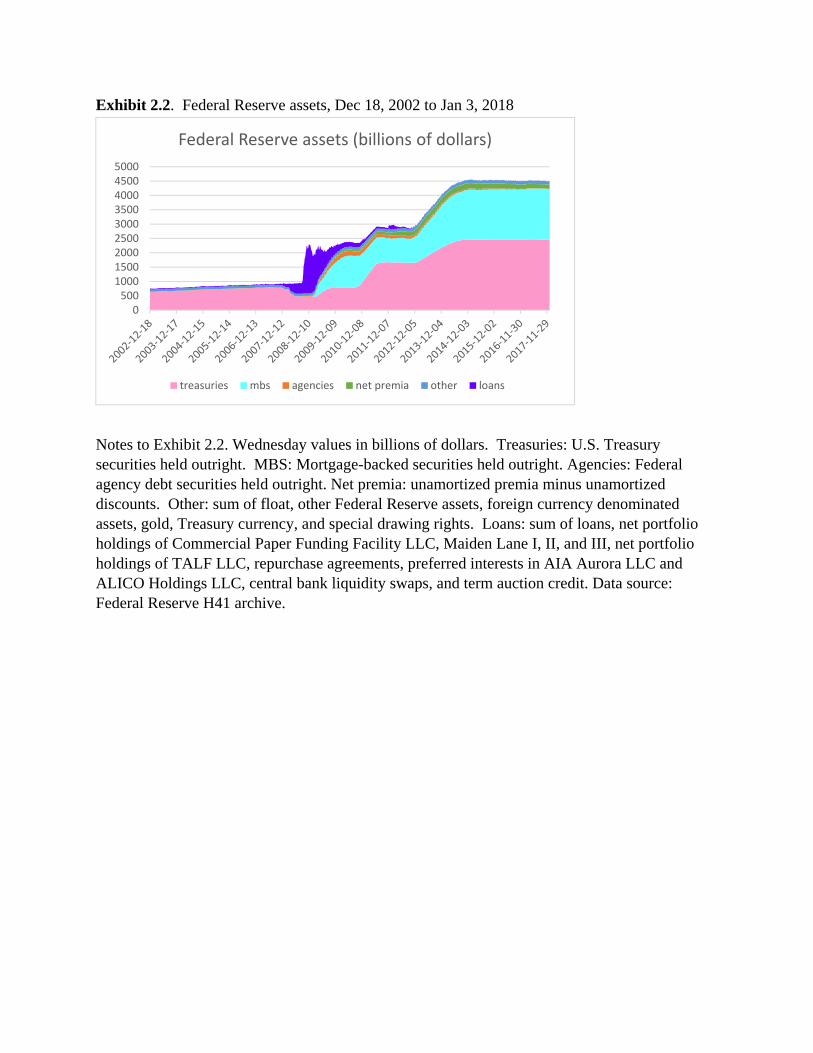
Exhibit 2.2. Federal Reserve assets, Dec 18, 2002 to Jan 3, 2018

Notes to Exhibit 2.2. Wednesday values in billions of dollars. Treasuries: U.S. Treasury securities held outright. MBS: Mortgage-backed securities held outright. Agencies: Federal agency debt securities held outright. Net premia: unamortized premia minus unamortized discounts. Other: sum of float, other Federal Reserve assets, foreign currency denominated assets, gold, Treasury currency, and special drawing rights. Loans: sum of loans, net portfolio holdings of Commercial Paper Funding Facility LLC, Maiden Lane I, II, and III, net portfolio holdings of TALF LLC, repurchase agreements, preferred interests in AIA Aurora LLC and ALICO Holdings LLC, central bank liquidity swaps, and term auction credit. Data source: Federal Reserve H41 archive.

0500100015002000250030003500400045005000

Federal Reserve assets (billions of dollars)

treasuries mbs agencies net premia other loans

Exhibit 2.3. Federal Reserve liabilities, Dec 18, 2002 to Jan 3, 2018

Notes to Exhibit 2.3. Wednesday values in billions of dollars. Currency: currency in circulation. Rev repo: Reverse repurchase agreements (foreign official and international accounts plus others). Term deposits: term deposits held by depository institutions. Treasury: U.S. Treasury general account plus supplementary financing account. Other: Treasury cash holdings plus foreign official, service-related and other deposits plus other liabilities and capital. Reserve balances: reserve balances with Federal Reserve banks. Data source: Federal Reserve H41 archive.

0500100015002000250030003500400045005000

Federal Reserve liabilities (billions of dollars)

currency rev repo term deposits treasury other reserve balances

Exhibit 3.1. Interest rates in Sweden (monthly averages, Jan 2013 to Dec 2017)

Notes to Exhibit 3.1. Data source: Riksbank.

‐1

‐0.5

0

0.5

1

1.5

2

2013 2014 2015 2016 2017

policy rate (repo) 3 month interbank rate

2‐year government bond 2 year mortgage rate

Exhibit 3.2. Policy rates (in red) and household and corporate bank deposit rates (blue or black) for Sweden, Denmark, Switzerland, and Japan

Notes to Exhibit 3.2. The policy rates are defined as the Repo Rate (Sweden), the Certificates of Deposit Rate (Denmark), SARON (Switzerland), and the Uncollaterized Overnight Call Rate (Japan). The red vertical lines mark the month in which policy rates became negative. Source: Eggertsson, Juelsrud, and Wold (2017).

Exhibit 3.3. Blue Chip consensus expected number of quarters until first federal funds rate increase (top-coded at 7 quarters)

Notes to Exhibit 3.3. Source: Swanson and Williams (2014).

Exhibit 3.4. Interest rate on constant-maturity 10-year Treasury bond

Notes to Exhibit 3.4. Rate implied by Chicago Board of Trade TNX contract, minute-by-minute observations (in Central Time) during March 18, 2009. Data source: Datastream.

2.4

2.5

2.6

2.7

2.8

2.9

3

3.1

9:00 10:12 11:24 12:36 13:48 15:00 16:12

Mar 18, 2009: 10‐year Treasury (TNX)

Exhibit 3.5. QE1 and QE2 announcements used by Krishnamurthy and Vissing-Jorgensen (2011) and change (in basis points) in yield on 10-year Treasuries in 2 days following announcement, on the day of the announcement, and within 30 minutes of the announcement

date  time  event  48 hour 

24 hour 

30 minute 

description 

QE1             

25‐Nov‐08  8:15  Fed press release 

‐36  ‐24  ‐3  The initial announcement that the Federal Reserve would purchase up to $100 billion of agency debt and up to $500 billion of agency MBS. 

1‐Dec‐08  13:45  speech  ‐25  ‐21  1  Chairman Bernanke's speech on the Federal Reserve Policies in the Financial Crisis, which suggested that the Federal Reserve could purchase longer‐term Treasury securities in substantial quantities in order to stimulate the economy. 

16‐Dec‐08  14:15  FOMC statement 

‐33  ‐16  ‐14  The Federal Reserve will continue to consider ways of using its balance sheet to further support credit markets and economic activity. 

28‐Jan‐09  14:15  FOMC statement 

28  12  1  The FOMC statement that was interpreted by some market participants as disappointing because of its lack of concrete language regarding the possibility and timing of purchases of longer‐term Treasuries in the secondary market. 

18‐Mar‐09  14:15  FOMC statement 

‐41  ‐51  ‐44  The FOMC statement, which announced purchases of Treasury securities of up to $300 billion and increased the size of purchases of agency MBS and agency debt to up to $1.2 trillion and $200 billion, respectively. 

Sum      ‐107  ‐100  ‐59   

            0 

QE2             

10‐Aug‐10  14:15  FOMC statement 

‐14  ‐7  ‐7  To help support economic recovery in the context of price stability, the Committee will keep the Federal Reserve's holdings of securities at their current level by reinvesting principal payments from agency debt and agency mortgage‐backed securities in longer‐term Treasury securities. The Committee will continue to roll over the Federal Reserve's holdings of Treasury securities as they mature. 

21‐Sep‐10  14:15  FOMC statement 

‐16  ‐10  ‐1  The FOMC is prepared to provide additional accommodation if needed. 

Sum      ‐30  ‐17  ‐8   

Exhibit 4.1. Bond yields tended to rise during the implementation of QE1, 2 and 3

Notes to Exhibit 4.1. The shaded area in this an all subsequent chart shows the period of balance sheet expansion: Jan 2009 to Mar 2010 for QE1, Nov 2010 to June 2011 for QE2 and Oct 2012 to Oct 2014 for QE3. Many of the announcement effects should come before or at the start of the shaded areas. Exhibit 4.2. Cumulative change in yields on all “Fed Days” ( meeting, minutes, chair speech)

Notes to Exhibit 4.12. The cumulative move is the sum of the actual change in yields on days of FOMC meetings, minute and Chair speeches and with zero for non-Fed Days. The cumulative change in this and all subsequent charts is in basis points.

0

500

1000

1500

2000

2500

3000

3500

4000

4500

-2

-1

0

1

2

3

4

5

6

06 07 08 09 10 11 12 13 14 15 16 17 18

Nominal yields Real yields Fed securities held outright ($bn, rhs)

-150

-100

-50

0

50

100

150

Oct-08 Oct-09 Oct-10 Oct-11 Oct-12 Oct-13 Oct-14 Oct-15 Oct-16 Oct-17

Nominal yields

Real yields

Exhibit 4.3. Cumulative change on Fed meeting days

Notes to Exhibit 4.3. Cumulative sum using actual yield changes on FOMC meeting days and zero for all other days.

Exhibit 4.4. Cumulative change on Fed minutes days

Notes to Exhibit 4.4. Cumulative sum using actual yield changes on days when the minutes were released and zero for all other days.

-140

-120

-100

-80

-60

-40

-20

0

Oct-08 Oct-09 Oct-10 Oct-11 Oct-12 Oct-13 Oct-14 Oct-15 Oct-16 Oct-17

Nominal yields

Real yields

-30

-20

-10

0

10

20

30

40

50

60

70

Oct-08 Oct-09 Oct-10 Oct-11 Oct-12 Oct-13 Oct-14 Oct-15 Oct-16 Oct-17

Nominal yields

Real yields

Exhibit 4.5. Cumulative change on Fed chair speech days

Notes to Exhibit 4.5. Cumulative sum using actual yield changes on days when the Chair gave and economic or policy related speech and zero for all other days.

Exhibit 4.6. Cumulative change in all non-Fed Days

Notes to Exhibit 4.6. Cumulative sum using actual yield changes on non-Fed Days and zero for all Fed Days.

-40

-20

0

20

40

60

80

Oct-08 Oct-09 Oct-10 Oct-11 Oct-12 Oct-13 Oct-14 Oct-15 Oct-16 Oct-17

Nominal yieldsReal yields

-400-350-300-250-200-150-100

-500

50100150

Oct-08 Oct-09 Oct-10 Oct-11 Oct-12 Oct-13 Oct-14 Oct-15 Oct-16 Oct-17

Nominal yieldsReal yields

Exhibit 4.7. Decomposing the net change into positive and negative moves

# days positive

change Cumulative

positive change # days negative

change Cumulative

negative change Total

Full sample Nominal 131 694.2 127 -676.3 17.9

until 12/06/17 Real 132 582.0 119 -658.2 -76.2

Expansion Nominal 73 427.9 68 -415.8 12.1

until 5/21/2013 Real 79 330.0 62 -379.3 -49.3

Exit Nominal 58 266.3 59 -260.5 5.8

from 5/22/2013 Real 53 252.0 57 -278.9 -26.9

Notes to Exhibit 4.7. Cumulative move in yields on Fed Days, divided into days when yields went up and days when yields went down. The first two rows show the cumulative move for our entire sample (starting in November 2008) and the later rows divide the sample with the day before Bernanke’s first taper tamper warning.

Exhibit 4.8. Events that moved the bond market significantly according to Reuters

Category Frequency Details

Fed 161 Balance Sheet (83), Interest Rate (80), Fed Purchase (16), Other (3)

Macro data 348 US economic data (348)

Europe 191 Economic/political news (135, ECB (37), European bonds (19)

Other international news 88 China (32), NK (6), Central banks(non-Fed/ECB) (14), Other countries (36)

Technicals/Supply 76 Technicals (28), Supply side news(48)

Stocks/Oil 65 Stock market movement (45), Oil price (20)

Continuation/Correction 75 Continuation (33), Correction (42)

US politics 50 US political news (50)

Other 71

Total 1125

 

Notes to Exhibit 4.8. The numbers in the details differ from the reported total frequency because some days contain more than one story. 

Exhibit 4.9. Nominal change on Reuters Fed News days and all other Reuters News days

Notes to Exhibit 4.9. The blue line is the cumulative change in yields when Reuters identified Fed news as a driver of markets, with zero for all other days. The yellow line shows the cumulative market move on all other Reuters days, with zero for all other days.

Exhibit 4.10. Cumulative change in yields for all days and for all non-Reuters Days

Notes to Exhibit 4.10. Recall that days with small moves (less than one standard deviation) are not included in out Reuters News day data set. This chart compares the cumulative move on these small movement days to the overall cumulative move in yields on all days.

-200

-150

-100

-50

0

50

100

150

Oct-08 Oct-09 Oct-10 Oct-11 Oct-12 Oct-13 Oct-14 Oct-15 Oct-16 Oct-17

Reuters Fed News All other news

-300

-250

-200

-150

-100

-50

0

50

Oct-08 Oct-09 Oct-10 Oct-11 Oct-12 Oct-13 Oct-14 Oct-15 Oct-16 Oct-17

Full sample range Non major-movement days

Exhibit 4.11. Decomposing the Reuters Fed News into balance sheet and interest rate news

Notes to Exhibit 4.11. This chart separates out the two kinds of Reuters Fed News days, showing cummulative moves for each. For reference it also shows the cummulaitve move in yields for all days in the sample. Exhibit 4.12.Other Reuters News days that caused large cummulative moves   

Notes to Exhibit 4.12. Our Reuters News data base captures all the days where the market moved at least one standard deviation. The chart shows the cumulative impact of US macro data announcements and developments in Europe.

-300

-250

-200

-150

-100

-50

0

50

Oct-08 Oct-09 Oct-10 Oct-11 Oct-12 Oct-13 Oct-14 Oct-15 Oct-16 Oct-17

Full sample range BS news IR news

-200

-150

-100

-50

0

50

100

150

Oct-08 Oct-09 Oct-10 Oct-11 Oct-12 Oct-13 Oct-14 Oct-15 Oct-16 Oct-17

Macro data Europe

Exhibit 4.13. Treasury debt management policy acted as an offset to Fed QE.

Notes to Exhibit 4.13. Source: Greenwood et al. (2014).

Exhibit 4.14. Real and nominal bond yields around QE1 announcements

Notes to Exhibit 4.14. Level of yields in percent. Shaded area covers the period from the first (November 25, 2008) to the second (March 18, 2009) QE1 announcement.

1.2

1.6

2.0

2.4

2.8

3.2

3.6

4.0

4.4

Aug-08 Oct-08 Dec-08 Feb-09 Apr-09 Jun-09 Aug-09

10-Year Inflation Indexed Yield 10-Year Yield

Exhibit 4.15. Change in 10 year yields on Reuters Fed Days under QE

Notes to Exhibit 4.15. Total bar heights denote change in 10 year yield on QE1 days for which Reuters report indicated at least some balance sheet component. Where interest rate guidance or other developments were also mentioned by Reuters, beige and orange shading was used in addition to the blue for balance sheet. F: FOMC meetings; B: Bernanke speeches; O: speeches by other FOMC members (O); M: minutes.

Exhibit 5.1. Nominal bond yields during the tantrum

Notes to Exhibit 5.1 10 year treasury yields around four major Fed signals: Bernanke’s two taper warnings, the failure to announce tapering at the September FOMC meeting and the actual announcement at the December meeting.

-60

-50

-40

-30

-20

-10

0

10

20

Nov25

Dec1

Dec16

Jan12

Jan14

Jan28

Feb18

Mar16

Mar18

Apr29

Jun24

Jul15

Jul21

Jul23

Aug12

Aug21

Sep23

Oct09

Oct14

Oct23

Nov4

BS IR Other

2008 2009F

OO

F

BF

M

FF

F

MO

B

M

B

F

B

F

OO F

1.5

1.7

1.9

2.1

2.3

2.5

2.7

2.9

3.1

3.3

Jan Feb Mar Apr May Jun Jul Aug Sep Oct Nov Dec

Bernanke 2

Sep FOMC

Dec FOMC

Bernanke 1

Exhibit 5.2. Implied balance sheet peak based on primary dealer survey

Notes to Exhibit 5.2. Respondents give the amount of Treasury and MBS purchases that would be in effect after various future FOMC meetings. We use the median responses to construct expectations about the total size of the QE3 program. For meetings that were omitted in the surveys, we fill out the missing data based on two principles: i) cuts to asset purchases would be initiated at a meeting with a press conference, and ii) unless the forecasts implied some tapering, asset purchases would be ended abruptly. We make the second assumption because it appears that respondents were not expecting asset purchases to be tapered until after Bernanke’s May 22, 2013 comments. The assumption implies slightly larger estimates of the total size of QE3, all else being equal.

Exhibit 5.3. Cumulative change in nominal bond yields during Taper Tantrum

Notes to Exhibit 5.3. Cumulative change in basis points from December 31, 2012 to December 31, 2013. Vertical line is drawn on May 21, the day before Bernanke’s first warning. Overall market is cumulative change on all days that year. Fed Days is the cumulative change on FOMC meeting days, the release of minutes and relevant Fed Chair speeches (with zero for all other days). Reuter Fed News is the same calculation allowing Reuters to pick the relevant Fed days.

800

900

1000

1100

1200

1300

1400

1500

1600

1700

1800

Oct-12 Dec-12 Jan-13 Mar -13 Apr- 13 Jun- 13 Jul -13 Sept- 13 Oct- 13 Dec-13

Expectations Actual

-20

0

20

40

60

80

100

120

140

Jan-13 Mar-13 May-13 Jul-13 Sep-13 Nov-13

Overall MarketFed daysReuter Fed News

Exhibit 5.4. Cumulative change in real bond yields during Taper Tantrum

Notes to Exhibit 5.4. Same as previous exhibit, but with real rather than nominal yields.

Exhibit 5.5. Causes of cumulative nominal bond yield changes during taper tantrum

Notes to Exhibit 5.5. Compares cumulative movement in nominal yields on three kinds of Reuters News days to the cumulative market movement on all days. Attribution to causes is based on Reuters news stories, as described in the text.

0

20

40

60

80

100

120

140

160

180

Jan-13 Mar-13 May-13 Jul-13 Sep-13 Nov-13

Overall Market

Fed days

Reuters Fed News

-40-20

020406080

100120140160

Jan-13 Mar-13 May-13 Jul-13 Sep-13 Nov-13

Overall Market Reuter Fed NewsUS Macro data Europe (broader measure)

Exhibit 5.6. Median expectations for balance sheet shrinkage

Primary dealer survey

Expectations (Jan 2017) Actual outcome Hawkish? Start shrinkage Jun-18 Oct-17 ✓ Balance sheet (yearend '19, $Bn) 3,770 3,598 ✓ Pause hiking Two meetings One meeting ✓ State contingent or preprogramed Uncertain Pre programed ✓

Blue Chip survey

Expectations (Jan 2017) Actual outcome Hawkish? Start shrinkage 2H 2018 Oct-17 ✓ Balance sheet (yearend '19, $Bn) 3,991 3,598 ✓ Pause hiking 1.5 meetings One meeting ✓ State contingent or preprogramed Uncertain Pre programed ✓

Note to Exhibit 5.6 Data are from Blue Chip and Federal Reserve Bank of New York. Neither survey asked investors whether they expected the Fed to announce its whole exit plan out of the gate.

Exhibit 5.7. Financial conditions index

Note to Exhibit 5.7. Source is the Federal Reserve Bank of Chicago

-2

-1

0

1

2

3

4

5

71 75 79 83 87 91 95 99 03 07 11 15

Exhibit 5.8. Fitted one-year forward treasury rate

Notes to Exhibit 5.8. Source Federal Reserve Board.

Exhibit 5.9. Causes of cumulative nominal yield change during shrinkage shrug

Note to Exhibit 5.9. The sample starts July 1, 2016. Attribution to causes is based on Reuters news stories, as described in the text.

0.4

0.8

1.2

1.6

2.0

2.4

Jan-16 Apr-16 Jul-16 Oct-16 Jan-17 Apr-17 Jul-17 Oct-17

-40

-20

0

20

40

60

80

100

120

140

Jul-16 Sep-16 Nov-16 Jan-17 Mar-17 May-17 Jul-17 Sep-17 Nov-17

Overall market Fed datesReuter Fed News Inflation dataUS politics

Exhibit 5.10. Causes of term premium changes during shrinkage shrug

Note to Exhibit 5.10. Term premium estimates are from Adrian, Crump and Moench (ACM), Federal Reserve Bank of New York. Attribution to causes is based on Reuters news stories, as described in the text.

Exhibit 6.1. Maximal monthly amounts by which the Fed will allow principal payments to reduce its holdings of Treasury securities and MBS

Treasuries MBS 2017:Q4 6 4 2018:Q1 12 8 2018:Q2 18 12 2018:Q3 24 16 2018:Q4 30 20

Exhibit 6.2. Maximal monthly amount by which the Fed will allow principal payments to reduce its holdings of Treasury securities and MBS and average monthly reductions expected to be realized by Bonis, Ihrig and Wei (2017)

cap drawdown 2018 Q1

20 17.7

Q2 30 28.5 Q3 40 33.0 Q4 50 37.2 2019-2021

50 30.0

-40

-20

0

20

40

60

80

100

Jul-16 Sep-16 Nov-16 Jan-17 Mar-17 May-17 Jul-17 Sep-17 Nov-17

Overall marketFed datesReuter Fed NewsInflation dataUS politics

Exhibit 6.3. Historical and projected Fed assets, Dec 18, 2002 to Dec 31, 2025

Exhibit 6.4. Historical and projected Fed liabilities, Dec 18, 2002 to Dec 31, 2025

0500100015002000250030003500400045005000

2002‐12‐18

2003‐12‐17

2004‐12‐15

2005‐12‐14

2006‐12‐13

2007‐12‐12

2008‐12‐10

2009‐12‐09

2010‐12‐08

2011‐12‐07

2012‐12‐05

2013‐12‐04

2014‐12‐03

2015‐12‐02

2016‐11‐30

2017‐11‐29

11/28/2018

11/27/2019

11/25/2020

11/24/2021

11/23/2022

11/22/2023

11/20/2024

11/19/2025

Federal Reserve assets (billions of dollars)

treasuries mbs agencies net premia other loans

0500100015002000250030003500400045005000

Federal Reserve liabilities (billions of dollars)

currency rev repo term deposits treasury other reserve balances

Exhibit 6.5. Treasury cash balance, daily, Jan 1, 2006 to Jan 26, 2018

Exhibit 6.6. Federal Reserve reverse repos, Wed values, Jan 6, 2010 to Jan 3, 2018

0

100

200

300

400

500

600

700

800

bil. $

Treasury cash balance

0

100

200

300

400

500

600

700

Reverse repos

Exhibit 6.7. Treasury financing gap, 2018 to 2027

Notes to Exhibit 6.7. Financing gap represents the amount that Treasury issuance must be increased based on an assumed budget deficit path. The budget path that is assumed here reflects the “Other Policies Extended” version of the estimates produced by the Committee for a Responsible Federal Budget on February 9, 2018 (following passage of the bipartisan spending package).Source: Author’s calculations based on CBO, CRFB, FRBNY and US Treasury data.

     

0

400

800

1200

1600

2000

2400

2018 2019 2020 2021 2022 2023 2024 2025 2026 2027

bil. $

Treasury debt managers face a sizable financing gap

SOMA Total Financing Gap

Exhibit 6.8. Weighted average maturity of outstanding marketable Treasury debt (in months)

Notes to Exhibit 6.8. Source: U.S. Treasury.

Exhibit 6.9. Cost of Treasury issuance at certain maturity points versus the variability of that cost

Notes to Exhibit 6.9. Source: TBAC

Exhibit 6.10. Actual Treasury issuance mix versus an optimal strategy derived from the TBAC model

Notes to Exhibit 6.10. Source: Treasury Department and TBAC.

Exhibit 6.11. Difference between 10 year and 2 year Treasury term premium

Notes to Exhibit 6.11. Shaded areas indicate NBER designated recession. Source: ACM term premia estimates, Federal Reserve Bank of New York.

Exhibit 6.12. Bills as a % of Treasury marketable debt outstanding

Notes to Exhibit 6.12. Source: MSPD, Bureau of Economic Analysis.

Exhibit 6.13. MBS redemptions after 2021 based on median scenario, 2022 to 2027

Notes to Exhibit 6.13. Source: FRBNY.

Exhibit 7.1. Fall in fed funds rate in recent U.S. recessions

Period Fall 1957:8-1958:6 2.3 1960:4-1961:4 2.4 1969:12-1971:1 4.8 1973:11-1975:5 4.8 1980:1-1980:9 3 1981:7-1983:1 10.4 1990:7-1991:5 2.4 2001:3-2002:1 3.6 2007:12-2009:8 4.1

average 4.2 Notes to Exhibit 7.1. Fall in monthly average effective fed funds rate between month recession began and two months after it ended.