a state transition matrix flight-test evaluation of sensor ......both extended kalman filter (ekf)...

Flight-Test Evaluation of Sensor

Fusion Algorithms for Attitude

Estimation

JASON N. GROSS, Student Member, IEEE

YU GU, Member, IEEE

MATTHEW B. RHUDY

SRIKANTH GURURAJAN

MARCELLO R. NAPOLITANO

West Virginia University

In this paper, several Global Positioning System/inertial

navigation system (GPS/INS) algorithms are presented using

both extended Kalman filter (EKF) and unscented Kalman

filter (UKF), and evaluated with respect to performance and

complexity. The contributions of this study are that attitude

estimates are compared with independent measurements provided

by a mechanical vertical gyroscope using 23 diverse sets of flight

data, and that a fundamental difference between EKF and UKF

with respect to linearization is evaluated.

Manuscript received January 16, 2011; revised May 16, 2011;

released for publication July 5, 2011.

IEEE Log No. T-AES/48/3/944006.

Refereeing of this contribution was handled by M. Braasch.

This work was supported in part by the West Virginia Department

of Highway under Project RP253-B.

Authors’ address: Department of Mechanical and Aerospace

Engineering, West Virginia University, 357 Engineering Sciences

Bldg., 395 Evansdale Dr., Morgantown, WV 26506, E-mail:

([email protected]).

0018-9251/12/$26.00 c° 2012 IEEE

NOMENCLATURE

A State transition matrix

a Acceleration in the body-axis frame (m/s2)

b Bias

b c Body-axis coordinate frame

c Statistical weighted linear regression bias

d Observation function input vector

e Statistical weighted linear regression error

f State transition function

g Acceleration due to gravity (m/s2)

H Observation matrix

h Observation function

i Sigma-point index

J Performance cost function

K Kalman gain matrix

k Discrete time index

L Dimension of augmented state vector

during prediction

l c Local geodetic coordinate frame

M Dimension of augmented state vector

during measurement update

n Measurement noise

P Error covariance matrix

p Roll rate (deg/s)

Q Process noise covariance matrix

q Pitch rate (deg/s)

R Measurement noise covariance matrix

r Yaw rate (deg/s)

u State transition function input vector

Vx, Vy, Vz Velocity in the local geodetic navigation

frame (m/s)

w Weight vector

x State vector

x,y,z Position in the local geodetic navigation

frame (m)

Y Output sigma points

y Output vector

z Measurement vector

μ Pitch angle (deg)

¸ Sigma-point scaling parameter

º Process noise

¾ Standard deviation

v Random walk variance

Á Roll angle (deg)

Â Sigma points

Ã Yaw angle (deg).

I. INTRODUCTION

The use of unmanned aerial vehicles (UAVs) for

civil applications has substantially increased in recent

years following the advancements of sensors and

microprocessors [1—5]. Within these applications,

accurate knowledge of attitude information is often

required [1, 4]; on the other hand, the overall system

weight and cost must be minimized [2, 5]. The

conflict between these two requirements prevents

2128 IEEE TRANSACTIONS ON AEROSPACE AND ELECTRONIC SYSTEMS VOL. 48, NO. 3 JULY 2012

the use of high quality inertial navigation systems

(INSs) typically used on military UAVs [3, 5].

Additionally, many applications have real-time

processing requirements [6], while others depend on

accurate postprocessing [7]. Therefore, there is a clear

need for developing algorithms that rely on low-cost

components and are evaluated with respect to both

accuracy and computational requirements.

For UAV-based remote sensing applications, such

as 3-D mapping with direct geo-referencing [8] or

constructing large image mosaics [7], high fidelity

aircraft attitude information is a key requirement.

In addition, in the application of airborne visual

target tracking, it was recently noted that tracking

error is most sensitive to attitude uncertainty [6].

Recent advances of micro-electro-mechanical systems

(MEMS) technology have made low-cost inertial

measurement units (IMUs) available; however, the

limited accuracy of these components does not make

them adequate alone due to the accumulation of

the sensor biases over time [9]. The high accuracy

of Global Positioning System (GPS) velocity

measurements has also lead researchers to develop

single GPS antenna-based attitude solutions. For

example, Kornfeld, Hansman, and Deyst [10, 11]

estimated aircraft pseudo-attitude based on only

GPS velocity measurements [10], and showed its

effectiveness toward detecting inertial sensor failures

[11]. The functional integration of a low-cost INS

and a GPS receiver has well-known benefits [12, 13].

The most notable advantage is that the unbiased

solution offered by a GPS receiver regulates the

low frequency drift associated with low-cost inertial

systems, and the high frequency errors present in

the GPS measurements are smoothed by inertial

measurements [14]. Several GPS/INS formulations

have been developed that vary in terms of the number

of navigation states estimated [14, 15] and the form

of GPS information used for measurement update

[16]. This paper focuses on investigating attitude

estimation solutions that rely on a loosely-coupled

[12] integration of low-cost GPS/INS sensors, in terms

of both accuracy and computational efficiency.

The nonlinearities associated with inertial

navigation equations often require the use of a

nonlinear estimator [15, 17, 18] in a GPS/INS sensor

fusion algorithm, to combine the information in a

predictor-corrector framework. Two popular nonlinear

estimators, the extended Kalman filter (EKF) [19]

and the unscented Kalman filter (UKF) [20], have

been applied to this problem [15—18], however,

there are still questions regarding their benefits and

drawbacks. Specifically, van der Merwe and Wan

[17] report superior estimation performance of UKF

over EKF in handling the nonlinearities present

in a GPS/INS application, while Crassidis reports

that UKF outperforms EKF for GPS/INS when

dealing with large initialization errors [15]. Wendel,

et al. state that significant performance increase

of UKF over EKF is found only when confronted

with large initialization errors, and essentially

no difference otherwise [16] in a tightly-coupled

GPS/INS sensor fusion application. Additionally,

with respect to computational requirements, van der

Merwe, et al. note that the computation complexity

order of the algorithms are the same [17], while St.

Pierre and Ing [21] contend, with empirical results,

that the UKF is computationally more expensive

than EKF. Furthermore, it has been stated that a

problem associated with EKF implementation is that

it is difficult to “tune” in comparison to the UKF

framework [20].

The above conflicting conclusions demonstrate that

many issues have yet to be fully addressed. Toward

improving the level of knowledge in this field, this

effort focuses on evaluating performances of multiple

GPS/INS sensor fusion algorithms using UAV flight

data with independent attitude “truth” measurements.

Specifically, instead of using simulated data for

performance analysis as in earlier comparison studies

[15—17], a total of 23 sets of flight data were selected,

from more than 150 data sets collected over seven

years using West Virginia University’s (WVU) three

jet-powered YF-22 UAVs [22], to represent diversity

in terms of operation temperature, wind conditions,

mission profile, and sensor payload configurations. In

each of these flights, a mechanical vertical gyroscope

is used to provide an independent measurement of

aircraft pitch and roll angles. These measurements are

used as truth data for comparison with aircraft attitude

angles estimated using different GPS/INS sensor

fusion algorithms. The goal of using several sensor

fusion formulations with a diverse set of flight data

is to gain deeper insights into the relative advantages

and disadvantages of applying either EKF or UKF to

GPS/INS based attitude estimation.

The rest of the paper is organized as follows.

Section II describes several GPS/INS sensor fusion

algorithms as well as some fundamental differences

between EKF and UKF implementations. Section III

discusses the experimental UAV sensor systems

and selected flight data. Section IV presents results

both with respect to the computational load and

estimation performance; finally, Section V provides

the conclusion of this study.

II. SENSOR FUSION ALGORITHMS

Most GPS/INS sensor fusion algorithms combine

two information sources for attitude estimation: the

time integration of rate gyroscopes and the known

direction of the Earth’s gravitational vector. In a static

setting, by referencing the Cartesian components of

Earth’s gravitational vector, 3-axis accelerometers can

be used as a tilt sensor to determine attitude [23]. In a

dynamic environment, however, accelerometers alone

GROSS, ET AL.: FLIGHT-TEST EVALUATION OF SENSOR FUSION ALGORITHMS FOR ATTITUDE ESTIMATION 2129

cannot distinguish between inertial and gravitational

accelerations. In these situations, a GPS receiver

can be used to provide information to isolate the

two acceleration components, and in this sense, the

GPS/accelerometers combination acts as a dynamic tilt

sensor.

Within this paper, several GPS/INS algorithms

are investigated. For each algorithm, Euler rotation

angles are estimated to provide a simple and intuitive

mathematical representation of aircraft attitude. This

was chosen over the singularity-free quaternion-based

attitude representation in order to avoid additional

algorithm complexities associated ensuring quaternion

unity norm requirement [24], and Euler angle

singularity points are rarely encountered within

many aerial UAV applications, and can be monitored

on-line [25].

A. Acceleration Vector Attitude Estimation (AVAE)

An acceleration vector attitude estimation (AVAE)

algorithm is developed for direct attitude estimation

following the dynamic tilt sensor concept. The

AVAE algorithm features GPS acceleration in a

local geodetic frame (l c), estimated by numerical

differentiation of GPS velocity measurements,

and accelerometer measurements obtained in the

aircraft body-axis (b c). The aircraft Euler angles,

roll (Á), pitch (μ), and yaw (Ã), define a direction

cosine matrix (DCM) between the two coordinate

frames [26]264axayaz

375(b c)

=

2641 0 0

0 cÁ sÁ

0 ¡sÁ cÁ

375264cμ 0 ¡sμ0 1 0

sμ 0 cμ

375

£

264 cÃ sÃ 0

¡sÃ cÃ 0

0 0 1

375264 ax

ay

az ¡ g

375(l c)

(1)

where a is acceleration and g is the acceleration due

to gravity. With measurements from both GPS and

accelerometers, the projection of the local gravity

vector on the three aircraft body-axes in terms of the

three Euler angles can then be solved, as demonstrated

by Kingston, et al. [14].

To reduce the matrix relationship shown in (1),

yaw angle (Ã) is approximated with the aircraft

heading angle (ª) which is directly obtained by

calculating the instantaneous four-quadrant inverse

tangent (e.g. atan 2) to the aircraft trajectory using

GPS velocity measurements in the x and y axes within

the (l c) coordinate frame:

Ã ¼ª = tan¡1ÃVy(l c)

Vx(l c)

!: (2)

The two remaining aircraft Euler angles are then

estimated by considering sequential Euler rotations.

Specifically, by considering the rotation through the

heading angle, an intermediate acceleration vector,

denoted with subscript (Ã), is defined as264axayaz

375(Ã)

=

264ax(l c) cosÃ+ ay(l c) sinÃay(l c) cosÃ¡ ax(l c) sinÃaz(l c)¡ g

375 (3)

which leads to the following algebraic equations:264axayaz

375(b c)

=

264 cosμ 0 ¡sinμsinÁsinμ cosÁ sinÁcosμ

cosÁsinμ ¡sinÁ cosÁcosμ

375

£

264axayaz

375(Ã)

: (4)

The first equation of the above set can be solved for

the pitch angle,

μ = tan¡1

0@ax(Ã)az(Ã) + ax(b c)

qa2x(Ã) + a

2z(Ã)¡ a2x(b c)

a2z(Ã)¡ a2x(b c)

1A :(5)

By again rotating the a(Ã) acceleration vector with the

newly obtained pitch estimate, a second intermediate

acceleration vector, denoted with subscript (Ã,μ),

leaves the roll angle as the only unknown variable,264axayaz

375(b c)

=

2641 0 0

0 cosÁ sinÁ

0 ¡sinÁ cosÁ

375264axayaz

375(Ã,μ)

(6)

which can be algebraically solved using

Á= tan¡1

0@¡ay(Ã,μ)az(Ã,μ)¡ ay(b c)

qa2y(Ã,μ) + a

2z(Ã,μ)¡ a2y(b c)

a2z(Ã,μ)¡ a2y(b c)

1A :(7)

Within the AVAE algorithm, the GPS

acceleration vector is calculated using a numerical

backward-difference derivative of the GPS velocity

measurement vector. To reduce the noise associated

with the numerical derivative, the pitch and roll

estimates obtained with the AVAE formulation are

smoothed with a first-order low-pass Butterworth

filter.

B. 3-State Sensor Fusion Formulation

While the AVAE algorithm provides estimates

of all three aircraft Euler angles, it does not take

advantage of information provided by low-cost rate

gyroscopes, which are readily available in MEMS

IMUs. In this context, a 3-state GPS/INS sensor

fusion algorithm is formulated as a state estimation

problem in a traditional predictor-corrector framework


with a Kalman filter (KF). Within this framework,

five major components are defined: a state vector x,an input vector u, a set of nonlinear state transition

functions f, a set of nonlinear observation functions h,

and a measurement vector z.In the 3-state formulation, the aircraft Euler angles,

denoted as x= [Á μ Ã]T, are first predicted using the

roll rate p, pitch rate q, and yaw rate r, measured

in the aircraft body-axis (b c) and denoted by u=[p q r]T(b c) using the relationships [27]:

_Á= (p+ qsinÁ tanμ+ rcosÁ tanμ) + ºÁ (8)

_μ = (qcosÁ¡ r sinÁ)+ ºμ (9)

_Ã = ((qsinÁ+ rcosÁ)secμ) + ºÃ (10)

where (8)—(10) are the nonlinear state transition

functions f(x,u,v), and v represents process noise.Next, a measurement-update procedure is performed,

which is conceptually equivalent to the AVAE

algorithm. Within this procedure, the triad of IMU

body-axis (b c) specific-force measurements d=

[ax ay az]T(b c) are transformed to the geodetic

frame (l c) using a DCM that defines the nonlinear

observation function, h(x,d,n), with the predictedattitude estimates provided by the rate gyros

264_Vx

_Vy

_Vz + g

375(l c)

=

264cÃcμ ¡sÃcÁ+cÃsμ sinÁ sÃsÁ+cÃsμcÁ

sÃcμ cÃcÁ+sÃsμsÁ ¡cÃsÁ+sÃsμcÁ¡sμ cμsÁ cμcÁ

375264axayaz

375(b c)

+ n (11)

where n represents the measurement noise;

the measurement vector z is acquired throughdifferentiation of GPS velocity measurements.

C. 9-State Sensor Fusion Formulation

In the 3-state formulation, the DCM relating

accelerometer measurements to GPS velocity is

used for regulating attitude estimates obtained by

integrating angular rate measurements from low-cost

gyroscopes. This requires nonlinear functions to

be present within both the state transition (8)—(10)

and observation functions (11). If both rate gyro

and accelerometer measurements are used for

estimating aircraft attitude, velocity, and position in

the prediction stage, then the measurement update is

linear, using directly the GPS position and velocity

measurements. This also removes the need for

numerical differentiation of the GPS velocity as in

AVAE and the 3-state formulation. Within this 9-state

formulation, the navigation state vector (x) considers afull position, velocity, and attitude (PVA) solution:

x= [xl c yl c zl c Vxl c Vyl c Vzl c Áb c μb c Ãb c]T

(12)

where the position and velocity are in the local

geodetic (l c) frame, and the Euler angles are in the

aircraft body axis (b c). The continuous-time state

transition equations f are given by

_x=

26666666666666666664

_x

_y

_z

_Vx_Vy

_Vz

_Á

_μ

_Ã

37777777777777777775

=

2666666666666666664

Vx

Vy

Vz

cÃcμax+(¡sÃcÁ+cÃsμsÁ)ay +(sÃsÁ+cÃsμcÁ)azsÃcμax+(cÃcÁ+sÃsμsÁ)ay +(¡cÃsÁ+sÃsμcÁ)az

¡sμax+cμsÁay +cμcÁaz ¡ gp+ qsÁtμ+ rcÁtμ

qcÁ¡ rsÁ(qsÁ+ rcÁ)secμ

3777777777777777775

+ º: (13)

In this sensor fusion formulation, the observation

function is linear

H = [I6£6 06£3] (14)

where the observation matrix simply extracts the

predicted position and velocity states,

y=Hx+ n (15)

to obtain an output vector, which is directly

comparable with the GPS measured position and

velocity: z= [xGPS yGPS zGPS VxGPS VyGPS VzGPS ]T(l c).


D. 15-State Sensor Fusion Formulation

Finally, a 15-state GPS/INS sensor fusion

formulation is developed by augmenting the 9-state

formulation with six time-varying bias states

associated with the six IMU measurements. This

approach has the added benefit of improving the

performance of the prediction stage (12), but at the

cost of added computational burden. The 15 estimated

states include PVA states and six sensor biases and are

given by

x= [xl c yl c zl c Vxl c Vyl c Vzl c

Áb cμb cÃb cbax bay baz bp bq br]T

(16)

where b stands for sensor bias. During the state

prediction procedure, the same relationships described

in (12) account for the first nine state transition

equations, with the exception that the bias states are

subtracted from the raw IMU measurements

u= [axb c¡ bax ayb c¡ bay azb c¡bazpb c¡ bp qb c¡bq rb c¡ br]T: (17)

In order to model the dynamics of the six bias states,

the random walk (RW) assumption is used,

_b = À (18)

which has been shown to apply to low-grade

MEMS-based sensors [28]. The variance of the

random noise v is determined based on each sensor’s

Allan variance as reported by the manufacturer.

The same measurement vector in the 9-state

formulation is also used for the 15-state measurement

update. The observation matrix is given by

H = [I6£6 06£9]: (19)

E. Nonlinear Estimators: Extended Kalman Filter andUnscented Kalman Filter

The algorithms associated with the EKF and the

UKF are well known and can be found in several

publications [13, 19, 29, 17]. Two fundamental

differences between EKF and UKF are summarized

as a difference with respect to the method employed

for linearization, and a difference in the way process

and measurement noises are implemented within each

algorithm. To facilitate this comparison, the EKF

and UKF algorithms are first discussed; next, the

distinctions between the two estimators are highlighted

with respect to their implications for the GPS/INS

sensor fusion formulations used in this study.

1) Extended Kalman Filter: For each GPS/INS

sensor fusion formulation, the continuous state

transition and observation functions are first

discretized. For the EKF, the nonlinear state transition

functions are used to predict the a priori state

estimates x̂kjk¡1:

x̂kjk¡1 = f(xk¡1jk¡1,uk)+ º (20)

where uk is the input vector to the state transitionfunction, and the additive process noise º is assumed

to be white, with a known covariance Q (i.e., º »N(0,Q)). A linearization of f is required to predict the

a priori error covariance matrix Pkjk¡1:

Pkjk¡1 = AkPk¡1jk¡1ATk +Q (21)

where Ak is the Jacobian matrix of f with respect to

xk¡1jk¡1.During the EKF measurement-update procedure,

the estimated outputs yk are directly comparableto the measurement vector zk. Using the nonlinear

observation functions, yk is calculated using

yk = h(xkjk¡1,dk)+ n (22)

where dk is the input vector to the observationfunctions, and n is the additive measurement noise,

assumed to be white Gaussian, with n»N(0,R). TheJacobian of the observation functions with respect to

xkjk¡1, Hk, is used to calculate the Kalman gain matrix,

Kk = Pkjk¡1HTk (HkPkjk¡1H

Tk +R)

¡1: (23)

Kk is then used to update the predicted states and error

covariance:

xkjk = xkjk¡1 +Kk(zk ¡ yk) (24)

Pkjk = (I¡KkHk)Pkjk¡1: (25)

2) Unscented Kalman Filter: UKF uses the

unscented transformation to transform statistical

information through nonlinear functions [20]. The

UKF prediction stage starts with the augmentation of

the state vector with the process noise xa = [xT ºT]T.The mean and error covariance matrix for the

augmented state vector is given as

x̄ak¡1jk¡1 = [xTk¡1jk¡1 0]T

Pak¡1jk¡1 =·Pk¡1jk¡1 0

0 Q

¸ (26)

which are then used to generate a set of sigma points

Âk¡1jk¡1 =hx̄ak¡1jk¡1 x̄ak¡1jk¡1 +¸

qPak¡1jk¡1

x̄ak¡1jk¡1¡¸qPak¡1jk¡1

i(27)

where ¸ is a scaling parameter. Next, each of the

sigma points is transformed through nonlinear state

transition functions:

Âi=0:2Lkjk¡1 = f(Âi=0:2Lk¡1jk¡1,uk) (28)

where L is the dimension of the augmented state

vector. With the transformed sigma points, the

predicted mean and error covariance are calculated


as weighted sums using

xkjk¡1 =2LXi=0

wmi Âikjk¡1 (29)

Pkjk¡1 =2LXi=0

wCi (Âikjk¡1¡ xkjk¡1)(Âikjk¡1¡ xkjk¡1)T:

(30)Details on assigning the weights and scaling

parameters for a UKF can be found in [17].

During a UKF measurement-update, the state

vector is augmented with the measurement noise

xa = [xT nT]T, and the predicted mean from (29) and

covariance from (30) are used to generate a new set of

sigma points:

x̄akjk¡1 = [xTkjk¡1 0]T, Pakjk¡1 =

·Pkjk¡1 0

0 R

¸(31)

Âkjk¡1 =hx̄akjk¡1 x̄akjk¡1 +¸

qPkjk¡1 x̄akjk¡1¡¸

qPkjk¡1

i(32)

which are then transformed through nonlinear

observation functions:

Yi=0:2Mk = h(Âikjk¡1,dk) (33)

where M is the dimension of the augmented state

vector. Subsequently, the outputs, the observation error

covariance, and the cross-covariance of the predicted

states and observations are calculated as weighted

sums of the transformed sigma points:

yk =

2MXi=0

wmi Yikjk¡1 (34)

Pyy =

Ã2MXi=o

wCi (Yik ¡ yk)(Yik ¡ yk)T

!(35)

Pxy =

Ã2MXi=o

wCi (Âikjk¡1¡ xkjk¡1)(Yik ¡ yk)T

!: (36)

Finally, the UKF Kalman gain is calculated using

Kk = PxyP¡1yy : (37)

The above gains are then used to update the predicted

states and error covariance:

xkjk = xkjk¡1 +Kk(zk ¡ yk) (38)

Pkjk = Pkjk¡1¡KkPyyKTk : (39)

A clear difference between EKF and UKF is the

use of analytical linearization by EKF as compared

with the use of statistical linearization [30, 31] within

UKF. Both 9-state and 15-state formulations presented

above have nonlinear state transition functions and

linear observation functions. Therefore, the EKF

and UKF implementations are different only during

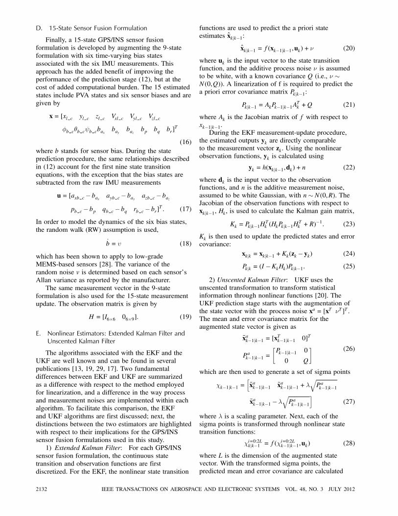
Fig. 1. YF-22 research UAV fleet.

the prediction step while the standard linear KF

measurement update procedure [19, 29] is used for

both filters. However, in the 3-state formulation,

nonlinearity is present in both the prediction and

update stages.

Another major difference between EKF and UKF

implementations presented is the method for handling

the process and measurement noise. Specifically,

within UKF, sigma points are generated according to

known or assumed statistical distributions of sensor

noise, which are then directly considered on the

sensor outputs and transformed through nonlinear

equations. This eliminates the need for additive

process and measurement noise assumptions. Instead,

EKF linearizes the nonlinear state transition and

observation equations only with respect to states,

and does not directly handle nonlinear relationships

with respect to sensor noise. As a result, EKF

implementation lumps different sources of noises

as one set of additive noise, whose property is

often difficult to determine in practical applications.

For example, in the relationships (8)—(10) used

in the prediction stage of all three sensor fusion

formulations, the overall process noise is a nonlinear

combination of rate gyroscope noises. In this case,

if it is assumed that the noise of each individual

rate gyroscope is white and Gaussian, the same

assumption is not necessarily valid for the overall

process noise. In general, it is possible to also derive a

Jacobian that linearizes the state transition function

about the assumed process noise within an EKF

implementation [32], however the ability for UKF

to easily handle noise at the sensor level though

statistically linearization nonlinear relationships

represents a practical implementation advantage over

EKF.

III. EXPERIMENTAL SET-UP

This sensor fusion study was conducted using

flight data collected on three WVU YF-22 research

platforms. Each aircraft, shown in Fig. 1, is

approximately 2.4 m long with a 2 m wing span, and

a weight of approximately 22.5 Kg. The aircraft is

powered with a miniature turbine that produces 125 N

of static thrust.


Fig. 2. YF-22 GPS/INS sensor fusion instrumentation.

The WVU YF-22 research platforms have been

utilized for various research projects, including the

validation of autonomous formation flight control

laws [33], and fault-tolerant flight control laws [34].

Over the years, a large database of flight data was

accumulated, which forms the foundation for this

study. A typical flight test involves manually piloted

and/or autonomous segments within a loitering loop

pattern.

Flight data were collected with two different

avionics architectures. Flights 1—21 were collected

with avionic system 1 [22], with Crossbow V400A®

IMUs and Novatel OEM4® GPS receivers. The

Crossbow IMUs were sampled with a 16-bit

resolution, over a full scale range of §200±=s on therate gyros, and §10 g for the accelerometers. TheOEM4 GPS receiver reports a 1.8 m circular error

probable (CEP) for position measurements. Avionic

system 2 [35] was used for Flights 22—23, on the blue

YF-22 (triangle indicates blue YF-22* in Fig. 3). An

Analog Devices ADIS-16405® IMU was used within

system 2, which provides a 14-bit digital output

Fig. 3. Flight data vs. temperature (top) and velocity distribution (bottom).

for all acceleration and rate channels, with range of

§150±=s for the gyros, and §18 g for theaccelerometers. The GPS within system 2 was also

a Novatel OEM4.

For both avionic systems, a Goodrich VG34®

mechanical vertical gyroscope was used to provide

independent pitch and roll angle measurements. The

VG34 has a §90± measurement range on the roll axisand a §60± range on the pitch axis, and was sampledwith 16-bit resolution. The VG34 has a self-erection

system, and reported accuracy of within 0:25± oftrue vertical. The output of the mechanical vertical

gyroscope was used as the truth data for the sensor

fusion study. The avionic system 2 is shown in Fig. 2.

Within this study, 23 sets of flight data were

considered, using three aircraft with four sets of

on-board sensor payloads. These flights were selected

from over 150 sets of flight data to represent a diverse

range of temperature conditions, wind conditions,

mission profile, and sensor platform. A distribution

of selected flight data with respect to operating

temperature and the research platform used is shown

in the top half of Fig. 4, and the velocity distribution

over the 23 flights are shown in the bottom half

of Fig. 3. Within the top plot in Fig. 3, the flights

numbers are ordered chronologically, and blue

YF-22* represents the blue YF-22 aircraft with

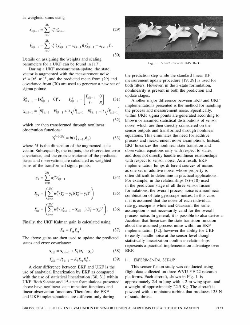
avionic system 2. The contour graph in Fig. 4 shows

the distribution of all data samples with respect

to pitch and roll angles, indicating dynamic flight

conditions and a large flight envelope covered over

the 23 flights.


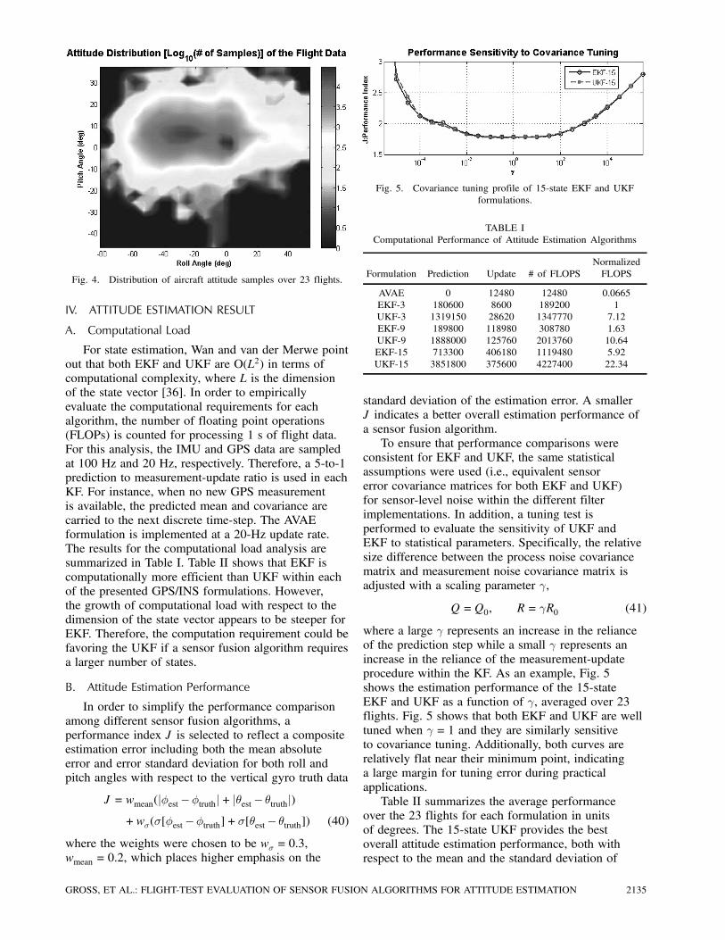
Fig. 4. Distribution of aircraft attitude samples over 23 flights.

IV. ATTITUDE ESTIMATION RESULT

A. Computational Load

For state estimation, Wan and van der Merwe point

out that both EKF and UKF are O(L2) in terms of

computational complexity, where L is the dimension

of the state vector [36]. In order to empirically

evaluate the computational requirements for each

algorithm, the number of floating point operations

(FLOPs) is counted for processing 1 s of flight data.

For this analysis, the IMU and GPS data are sampled

at 100 Hz and 20 Hz, respectively. Therefore, a 5-to-1

prediction to measurement-update ratio is used in each

KF. For instance, when no new GPS measurement

is available, the predicted mean and covariance are

carried to the next discrete time-step. The AVAE

formulation is implemented at a 20-Hz update rate.

The results for the computational load analysis are

summarized in Table I. Table II shows that EKF is

computationally more efficient than UKF within each

of the presented GPS/INS formulations. However,

the growth of computational load with respect to the

dimension of the state vector appears to be steeper for

EKF. Therefore, the computation requirement could be

favoring the UKF if a sensor fusion algorithm requires

a larger number of states.

B. Attitude Estimation Performance

In order to simplify the performance comparison

among different sensor fusion algorithms, a

performance index J is selected to reflect a composite

estimation error including both the mean absolute

error and error standard deviation for both roll and

pitch angles with respect to the vertical gyro truth data

J = wmean(jÁest¡Átruthj+ jμest¡ μtruthj)+w¾(¾[Áest¡Átruth]+¾[μest¡ μtruth]) (40)

where the weights were chosen to be w¾ = 0:3,

wmean = 0:2, which places higher emphasis on the

Fig. 5. Covariance tuning profile of 15-state EKF and UKF

formulations.

TABLE I

Computational Performance of Attitude Estimation Algorithms

Normalized

Formulation Prediction Update # of FLOPS FLOPS

AVAE 0 12480 12480 0.0665

EKF-3 180600 8600 189200 1

UKF-3 1319150 28620 1347770 7.12

EKF-9 189800 118980 308780 1.63

UKF-9 1888000 125760 2013760 10.64

EKF-15 713300 406180 1119480 5.92

UKF-15 3851800 375600 4227400 22.34

standard deviation of the estimation error. A smaller

J indicates a better overall estimation performance of

a sensor fusion algorithm.

To ensure that performance comparisons were

consistent for EKF and UKF, the same statistical

assumptions were used (i.e., equivalent sensor

error covariance matrices for both EKF and UKF)

for sensor-level noise within the different filter

implementations. In addition, a tuning test is

performed to evaluate the sensitivity of UKF and

EKF to statistical parameters. Specifically, the relative

size difference between the process noise covariance

matrix and measurement noise covariance matrix is

adjusted with a scaling parameter °,

Q =Q0, R = °R0 (41)

where a large ° represents an increase in the reliance

of the prediction step while a small ° represents an

increase in the reliance of the measurement-update

procedure within the KF. As an example, Fig. 5

shows the estimation performance of the 15-state

EKF and UKF as a function of °, averaged over 23

flights. Fig. 5 shows that both EKF and UKF are well

tuned when ° = 1 and they are similarly sensitive

to covariance tuning. Additionally, both curves are

relatively flat near their minimum point, indicating

a large margin for tuning error during practical

applications.

Table II summarizes the average performance

over the 23 flights for each formulation in units

of degrees. The 15-state UKF provides the best

overall attitude estimation performance, both with

respect to the mean and the standard deviation of


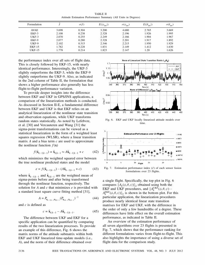
TABLE II

Attitude Estimation Performance Summary (All Units in Degrees)

Formulation J̄ ¾(J) E(jÁerrj) ¾(Áerr) E(jμerrj) ¾(μerr)

AVAE 3.698 0.304 3.200 4.680 2.765 3.669

EKF-3 2.108 0.238 2.328 2.196 1.926 1.995

UKF-3 2.070 0.255 2.249 2.166 1.904 1.967

EKF-9 2.077 0.280 2.328 2.201 1.917 1.892

UKF-9 2.102 0.315 2.346 2.215 1.950 1.929

EKF-15 1.782 0.228 1.831 2.149 1.412 1.630

UKF-15 1.778 0.214 1.823 2.147 1.20 1.626

the performance index over all sets of flight data.

This is closely followed by EKF-15, with nearly

identical performance. Interestingly, the UKF-3

slightly outperforms the EKF-3, while the EKF-9

slightly outperforms the UKF-9. Also, as indicated

in the 2nd column of Table II, the formulation that

shows a higher performance also generally has less

flight-to-flight performance variation.

To provide deeper insights into the difference

between EKF and UKF in GPS/INS applications, a

comparison of the linearization methods is conducted.

As discussed in Section II-E, a fundamental difference

between EKF and UKF is that EKF relies on an

analytical linearization of the nonlinear state transition

and observation equations, while UKF transforms

random states statistically. As noted by Lefebvre,

et al. [30] and Vercauteren and Wang [31] the

sigma-point transformations can be viewed as a

statistical linearization in the form of a weighted least

squares regression (WLSR), where a linear transition

matrix A and a bias term c are used to approximate

the nonlinear function f(x)

f(x̄k¡1jk¡1) = x̄kjk¡1 ¼ Ax̄k¡1jk¡1 + c (42)

which minimizes the weighted squared error between

the true nonlinear predicted states and the model

e= f(x̄k¡1jk¡1)¡ (Ax̄k¡1jk¡1 + c) (43)

where x̄k¡1jk¡1 and x̄kjk¡1 are the weighted mean ofsigma-points before and after being transformed

through the nonlinear function, respectively. The

solution for A and c that minimizes e is provided with

a standard least square curve fitting method [31],

A= Pxk¡1jk¡1xkjk¡1 (Pxkjk¡1xkjk¡1 )¡1 (44)

and c is defined as

c= x̄kjk¡1¡Ax̄k¡1jk¡1: (45)

The difference between UKF and EKF for a

specific application can be quantified by comparing

results of the two linearization processes. To provide

an example of this difference, Fig. 6 shows the

matrix norms of the attitude submatrix within both

EKF and UKF linearized time-update models (i.e.,

A), and the norm of their difference obtained over

Fig. 6. EKF and UKF locally linearized attitude models over

time.

Fig. 7. Estimation performance index (J) of each sensor fusion

formulations over 23 flights.

a single flight. Specifically, the top plot in Fig. 6

compares kAk(Á,μ,Ã)k2 obtained using both theEKF and UKF procedures, and kAUKFk (Á,μ,Ã)¡AEKFk (Á,μ,Ã)k2 is shown in the bottom plot. For this

particular application, the linearization procedures

produce nearly identical linear state transition

matrixes for EKF and UKF, with the difference in

the order of only a few hundredths of a degree. These

differences have little effect on the overall estimation

performance, as indicated in Table II.

An overview of the estimation performance of

all seven algorithms over 23 flights is presented in

Fig. 7, which shows that the performance ranking for

different formulations varies from flight-to-flight. This

also highlights the importance of using a diverse set of

flight data for the comparison study.


V. CONCLUSIONS

In small UAV-based applications the performance

of sensor fusion algorithms often reflects a tradeoff

between accuracy and the availability of on-board

computational resources. Following a detailed

comparative analysis, the AVAE has shown to be the

most computationally efficient algorithm; therefore,

it is considered to be more suitable for a low-cost

real-time attitude reference system. Furthermore, the

AVAE algorithm does not use a nonlinear estimator,

which further eases implementation and tuning

requirements. The EKF-3 offers a good balance

between estimation performance and computational

load. As shown in Table II, the EKF-3 ranks in the

middle in terms of estimation performance, but is

second only to AVAE in terms of computational

requirements. While computationally expensive, the

UKF-15 most closely matches the vertical gyroscope

measurements. This formulation provides an excellent

postprocessing solution.

This study utilized 23 diverse sets of flight data

collected with four separate sensor systems with

independent attitude truth measurement. A comparison

analysis shows that EKF and UKF provide similar

estimation performance throughout various GPS/INS

attitude estimation formulations. In addition, within

this application, EKF and UKF showed similar

performance sensitivity with respect to process

noise/measurement noise covariance tuning. Finally,

with respect to the nonlinear state transition functions

used for attitude estimation, the linearization methods

employed by EKF and UKF were shown to produce

very similar instantaneous linear models. Because

the performance differences between EKF and UKF

are minor, yet the computational requirements are

very different, the EKF shows to be the most suitable

nonlinear filtering solution for GPS/INS sensor fusion

based attitude estimation. This claim is substantiated

by the fact that the EKF-15 is significantly less

computationally complex than even the UKF-3.

REFERENCES

[1] Changchun, L., et al.

The research on unmanned aerial vehicle remote sensing

and its applications.

Proceedings of the IEEE 2010 International Conference on

Advanced Computer Control (ICACC), Shenyang, China,

2010, pp. 644—647.

[2] Dascalu, S.

Remote sensing using autonomous UAVs suitable for less

developed countries.

The International Archives of the Photogrammetry, Remote

Sensing and Spatial Information Sciences, 34 (May 2006).

[3] Everaerts, J.

The use of unmanned aerial vehicles (UAVs) for remote

sensing and mapping.

The International Archives of the Photogrammetry, Remote

Sensing and Spatial Information Sciences, XXXVI, B1

(2008), 1187—1192.

[4] Jensen, A., Baumann, M., and Chen, Y.

Low-cost multispectral aerial imaging using autonomous

runway-free small flying wing vehicles.

Proceedings of the IEEE International Geoscience and

Remote Sensing Symposium (IGARSS), Boston, MA,

2008, pp. 506—509.

[5] Zhou, G. and Zang, D.

Civil UAV system for Earth observation.

Proceedings of the IEEE International Geoscience and

Remote Sensing Symposium (IGARSS), Barcelona, Spain,

2007.

[6] Han, K. and DeSouza, G. N.

Instantaneous geo-location of multiple targets from

monocular airborne video.

Proceedings of the 2009 IEEE International Geoscience

and Remote Sensing Symposium (IGARSS), Cape Town,

South Africa, July 2009, pp. IV 1003—1006.

[7] Suzuki, T., Amano, Y., and Hashizym, T.

Vision based localization of a small UAV for generating a

large mosaic image.

Proceedings of 2010 SICE Annual Conference, Taipei, Oct.

2010, pp. 2960—2964.

[8] Nagai, M., et al.

UAV-borne 3-D mapping system by multisensor

integration.

IEEE Transactions on Geoscience and Remote Sensing, 47,

3 (Mar. 2009), 701—708.

[9] El-Diasty, M. and Pagiatakis, S.

A rigorous temperature-dependent stochastic modelling

and testing for MEMS-based inertial sensor errors.

MDPI, 9 (2009), 8473—8489, ISSN 1324-8220.

[10] Kornfeld, R. P., Hansman, R. J., and Deyst, J. J.

Preliminary flight tests of pseudo-attitude using single

antenna sensing.

Proceedings of the 17th Digital Avionics Systems

Conference (AIAA/IEE/SAE), vol. 1, Bellevue, WA,

1998, pp. E56/1—E56/8, ISBN 0-7803-5086-3.

[11] Deyst, J. J., Kornfeld, R. P., and Hansman, R. J.

Single antenna GPS information based aircraft attitude

redundancy.

Proceedings of the American Control Conference, vol. 5,

San Diego, CA, 1999, pp. 3127—3131.

[12] Grewal, M. S., Weill, L. R., and Andrew, A. P.

Global Positioning, Inertial Navigation & Integration (2nd

ed.).

Hoboken, NJ: Wiley, 2007.

[13] Kaplan, E. and Heagarty, C.

Understanding GPS Principles and Applications (2nd ed.).

Norwood, MA: Artech House, 2006.

[14] Kingston, D. B. and Beard, R. W.

Real-time attitude and position estimation for small UAVs

using low-cost sensors.

AIAA 3rd Unmanned Unlimited Systems Conference and

Workshop, Chicago, IL, Sept. 2004, AIAA-2004-6488.

[15] Crassidis, J.

Sigma-point filtering for integrated GPS and inertial

navigation.

AIAA Guidance, Navigation and Control Conference and

Exhibit, San Francisco, CA, 2005.

[16] Wendel, J., et al.

A performance comparison of tightly coupled GPS/INS

navigation systems based on extended and sigma point

Kalman filters.

Navigation: Journal of the Institute of Navigation, 53, 1,

(Spring 2006).


[17] van der Merwe, R., Wan, E., and Julier, S.

Sigma-point Kalman filters for nonlinear estimation and

sensor fusion–Applications to integrated navigation.

AIAA Guidance, Navigation and Control Conference,

Providence, RI, 2004, pp. 2004-5120.

[18] Gross, J., et al.

A comparison of extended Kalman filter, sigma-point

Kalman filter, and particle filter in GPS/INS sensor

fusion.


Exhibit, Toronto, Canada, 2010.

[19] Stengel, R. F.

Optimal Control and Estimation.

New York: Dover, 1994.

[20] Julier, S. and Uhlmann, J.

A new extension of the Kalman filtering to nonlinear

systems.

Proceedings of SPIE, vol. 3069, 1997, pp. 50—62.

[21] St. Pierre, M. and Ing, D.

Comparison between the unscented Kalman filter and the

extended Kalman filter for the position estimation module

of an integrated navigation information system.

IEEE Intelligent Vehicles Symposium, Parma, Italy, 2004.

[22] Gu, Y., et al.

Autonomous formation flight: Hardware development.

IEEE Mediterranean Control Conference, Ancona, Italy,

June 2006.

[23] Luczak, S., Oleksiuk, W., and Bodnicki, M.

Sensing tilt with MEMS accelerometers.

IEEE Sensors, 6, 6 (Dec. 2006), 1669—1673.

[24] Crassidis, J. L., Markley, F. L., and Cheng, Y.

A survey of nonlinear attitude filtering methods.

AIAA Journal of Guidance, Control and Dynamics, 30, 1

(Jan.—Feb. 2007), 12—28.

[25] Singla, P., Mortari, D., and Junkins, J.

How to avoid singularity for Euler angle set?

AAS 2004 Space Flight Mechanics Meeting Conference,

Maui, HI, Feb. 9—13, 2004, AAS 04-190.

[26] Stevens, B. L. and Lewis, F. L.

Aircraft Control and Simulation (2nd ed.).


[27] Roskam, J.

Airplane Flight Dynamics and Automatic Flight Controls.

DARcorporation, Lawrence, KS, 2003.

Jason N. Gross (S’11) was born in Charleston WV in 1985. In 2007, he receivedhis Bachelor of Science in mechanical engineering and a Bachelor of Science in

aerospace engineering. from West Virginia University, Morgantown, WV.

Since 2008, he has been a graduate research assistant at West Virginia

University working towards a Ph.D. in aerospace engineering, and since 2009

he has been a NASA WV Space Grant Consortium graduate research fellow.

He interned at NASA Goddard Space Flight Center in the summers of 2005 and

2007.

Mr. Gross is a student member of AIAA.

[28] El-Diasty, M. and Pagiatakis, S.

Calibration and stochastic modeling of inertial navigation

sensor errors.

Journal of Global Positioning Systems, 7, 2 (2008),

170—182.

[29] Crassidis, J. and Junkins, J.

Optimal Estimation of Dynamic Systems.

New York: Chapman & Hall/CRC, 2004.

[30] Lefebvre, T., Bruyninckx, H., and De Schuller, J.

Comment on “A new method for the nonlinear

transformation of means and covariances in filters and

estimators.”

IEEE Transactions on Automatic Control, 47, 8 (2002),

1406—1409.

[31] Vercauteren, T. and Wang, X.

Decentralized sigma-point information filters for target

tracking in collaborative sensor networks.

IEEE Transactions on Signal Processing, 53, 8 (Aug.

2005).

[32] Simon, D.

Optimal State Estimation.


[33] Gu, Y., et al.

Autonomous formation flight–design and experiments.

In Aerial Vehicles, I-Tech Education and Publishing,

Austria, Jan. 2009, ch. 12, pp. 233—256, ISBN

978-953-7619-41-1.

[34] Gu, Y.

Design and flight testing actuator failure accommodation

controllers on WVU YF-22 research UAVs.

Ph.D. dissertation, Dept. of Mechanical and Aerospace

Engineering, West Virginia University, 2004.

[35] Gross, et al.

Advanced research integrated avionics (ARIA) system for

fault-tolerant flight research.


Exhibit, Chicago, 2009.

[36] Wan, E. and van der Merwe, R.

The unscented Kalman filter for nonlinear estimation.

Proceedings of IEEE 2000 AS-SPCC Symposium, Lake

Louise, Alberta, CA, 2000.


Yu Gu (M’04) was born in Huainan, China in 1975. He received a B.S. degree in

automatic controls from Shanghai University in 1996, an M.S. degree in control

engineering from Shanghai Jiaotong University in 1999, and a Ph.D. degree in

aerospace engineering from West Virginia University, Morgantown, in 2004.

Since 2005 he has been a research assistant professor in the Department of

Mechanical and Aerospace Engineering at West Virginia University. His main

research interests include sensor fusion, flight control, and small unmanned aerial

vehicle (SUAV) design, instrumentation, and flight testing.

Matthew B. Rhudy received a Bachelor of Science in mechanical engineering in2008 from The Pennsylvania State University, State College, PA, and a Master

of Science in mechanical engineering in 2009 from the University of Pittsburgh,

Pittsburgh, PA.

Since 2010, he has been working towards a Ph.D. in aerospace engineering as

a graduate research assistant at West Virginia University, Morgantown, WV. He

worked as a graduate student researcher at the University of Pittsburgh from 2008

to 2009, an undergraduate teaching intern at The Pennsylvania State University

from 2007 to 2008, and a quality engineering intern in the summer of 2007 for

Tyco Electronics.

Mr. Rhudy is currently a student member of AIAA.

Srikanth Gururajan received his Ph.D. degree in aerospace engineering fromWest Virginia University, Morgantown, in 2006.

He is currently working as a post-doctoral fellow in the Department of

Mechanical and Aerospace Engineering at West Virginia University.

Dr. Gururajan is a senior member of the AIAA.

Marcello R. Napolitano was born in Pomigliano d’Arco, Italy, in 1961. Heholds a Master degree in aeronautical engineering from the ‘Universita’ di

Napoli—Federico II’, Naples, Italy, in 1985 and a Ph.D. in aerospace engineering

from Oklahoma State University, Stillwater, OK, in 1989.

He is currently a professor in the Department of Mechanical and Aerospace

Engineering (MAE), West Virginia University. He is also the Director of the

Flight Control System Research Laboratory in the MAE Department at WVU.

Dr. Napolitano is the author or coauthor of more than 130 technical

publications in the general area of fault tolerant flight control systems and

UAV-related research. Additionally, he is the author of the textbook, Aircraft

Dynamics: From Modeling to Simulation (Wiley, 2011). He is a member of the

AIAA.


a state transition matrix flight-test evaluation of sensor ......both extended kalman filter (ekf)...

Documents