a strategy for speed dating - lexjansen.com

1

A strategy for speed Dating YuTing Tian

ABSTRACT

Online dating is a growing industry with recent quarterly profits well in excess of millions. The goal of speed dating is to break into this industry by using the power of statistics to optimally match couples.

In order to attain this target, we will use a speed dating dataset to generate models to test feasibility of using statistics to match couples. This dataset is an open source on R package. The participants were students at Columbia’s graduate and professional schools, recruited by mass email, posted fliers, and fliers handed out by research assistants. Each participant attended one speed dating session, in which they met with a participant of the opposite sex for four minutes. Order and session assignments were randomly determined. After each four minute ”speed dating” encounter , participants filled out a form rating their date on scale of 1 to 10 on various attributes.

In this paper I use R software to download the dataset package, then use SAS® to analyze the data.

INTRODUCTION

In this paper, the author acknowledges that some of the figures are small; t is suggested that a reader might download the PDF and print the paper .

This paper is divided into the following four main sections:

1) Brief introduction for the speed dating data.

2) Some Basic Hypothesis

2.1) Impact of race2.2) Impact of age range

2.3) the correlation between like ratings and other independent variables

3) Building a model

3.1) Strategy to build the model

3.2) Collinearity test for the candidate model

3.3) Regression diagnostics for the final model

3.4) reliability evaluation for the final model

4) Conclusion

2

1) BRIEF INTRODUCTION FOR OUR SPEED DATING DATA

First the original dataset was cleaned, for example, converting the “NA” in the character variable, to missing value in the numerical variable (see Appendix), all the polynomial and interaction variables were added, for example Ambitious2=Ambitious**2, AA3=Attractive*Ambitious.

Then I split the data into two parts: training dataset 1/3 and test dataset 2/3

The chart in Figure 1 presents all the variables in the dataset. The target variables (likef likem) ( numeric), indicating how much do you like this person

Figure1 For each couple, 10 pair of input variables were recorded, for example AmbitiousF, AmbitiousM, with

each variable having a scale from 1 to 10. we will want to use each variable in the modeling to determine as a match Each dater’s scale is from 0 to 10 based on the opinion of the person, as indicated by the like variable. based on the attractiveness, sincerity, Intelligence, Fun, ambitious and shared interest of their partner

2) SOME BASIC HYPOTHESIS

2.1) IMPACT OF RACE

The first test to be performed is the effect of same race on the Like variable

3

Figure 2

From the cross-tabulation above, we see there are 80 same-race couples (Figure 2).

Our model then looks like:

Model: like=β0+β1*diff_race;

where the β0 is the intercept and β1 is the first regression coefficient; measures how difference with the predicted value of Like will to be while the partners are the same race. I create the dummy variable called diff_race, among partners, when female’s race different with male’s race, the diff_race equals to 1; otherwise, the diff_race equals to 0.

Then, the Null hypothesis (H0) means there is no significant relationship between a partner of different race and like variable; otherwise, the alternative hypothesis (Ha) means there is significant relationship between a partner of different race and like variable existed in this case.

Figure 3

I run the regression model, from the figure 3, we see the intercept is 6.5469, it means the expected value of “like” is 6.5469 when a partner’s race is the same.

4

Then, we see the coefficient of diff_race is -0.0639, it means on average, the expected value of “like” will be 0.0639 less when a partner’s race is the difference

We see the P value is 0.7517, greater than 0.05; it means there is no significantly difference on average “like” value whether race is the same or not. Then we accept the null hypothesis, because there is no significantly different.

2.2) THE IMPACT OF AGE RANGE

The second test to be performed the effect of age range on the Like variable. The same age range is defined by being within 2 years of one another.

The model then looks like:

Model: like=β0+β1*diff_age;

where the β0 is the intercept when the independent variables are equal to 0. β1 is the first regression coefficient, measures the difference with the predicted value of “like” when the partners are the same age range or not. binary dummy variable, diff_age, was created when the partner’s the same age range within 2 years, the value 1; otherwise 0;

Then, the Null hypothesis (H0) means there is no significant relationship between a partner of different age range and like variable; otherwise, the alternative hypothesis (Ha) means there is significant relationship between a partner of different age range and like variable

Figure 4

The regression model, shown figure 4 . we see the intercept is 6.6691, it means the expected value of “like” is 6.6691 when a partner’s age range is the same.

Then, we see the coefficient of diff_race is -0.2517, it means on average, the expected value of “like” will be 0.2517 lower when a partner’s age range is different. We see the P value is 0.2235, greater than 0.05; it means there is no significantly different on average “like” value whether the partner has same age range or not. Therefore, we will accept the H0

2.3) THE CORRELATION BETWEEN LIKE RATINGS AND OTHER INDEPENDENT VARIABLES

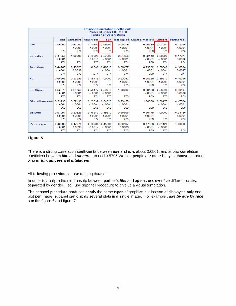
I want to see the whole correlation between independent variables and like without taking account into the factor gender, Therefore I get the mean ratings for selected predictor variables on each couple. Then create the Pearson Correlation Coefficient table shown on the figure 5;

5

Figure 5

There is a strong correlation coefficients between like and fun, about 0.6861; and strong correlation coefficient between like and sincere, around 0.5705 We see people are more likely to choose a partner who is fun, sincere and intelligent.

.

All following procedures, I use training dataset;

In order to analyze the relationship between partner’s like and age across over five different races, separated by gender. , so I use sgpanel procedure to give us a visual temptation.

The sgpanel procedure produces nearly the same types of graphics but instead of displaying only one plot per image, sgpanel can display several plots in a single image. For example , like by age by race, see the figure 6 and figure 7

6

Figure 6

Figure 6 shows how the relationship looks like between females’ ages and male’s like across over different female races. We see on average, the extent of men’s like almost the same as women’s ages growing, when the women’s race are Asian. But the shadow of 95% confidence interval is wider as women’s ages go up. It means the distribution of men’s like are spread above and beyond the predicted value. As ages growing, the variance becomes greater In addition, we see the extent of man’s like drops down as woman’s age goes up over across the other races.

7

Figure 7

Figure 7 is similar as Figure 6, showing man’s opinion to woman. We see on average, the extent of men’s like are increased gradually as women’s age growing, when the women’s race is Caucasian. Thereafter, we see the extent of men’s like is declined as women’s ages rise up over across the other races.

3) BUILDING A MODEL

3.1) STRATEGY TO BUILD THE MODEL

When we face with a predicted modeling problem, we use statistical model selections searching for the best model. Methods include long familiar in the Reg procedure (all possible subsets regression, forward selection, backwards elimination, and stepwise forward selection). I will use these four different strategies to create different models for two reasons.

The first reason is to try and create enough examples so that the effect of different parameters could be deduced from different methods.

The second reason is that different strategy has its own procedure:

For the all possible subsets regression procedure, identify all possible regression models derived from all possible combinations of independent variable. With many independent variables, the number of combinations would be unwieldy.

For the forward selection method, it starts with no variable in the model. For each of independent variable, the forward method calculates F statistics that reflects the variable’s contribution to the model. If the p value of F statistics has a significance level greater than the SLENTRY= value, the forward selection will be stopped otherwise the forward method adds this variable into the model.

8

Therefore, variables are added one at a time and remain in the model if they produce a significant F statistics. I set up the SLENTRY=0.05 in this method, because I want the variables whose significant values less than 0.05 can be added in the model. In the majority of analysis, an alpha is 0.05 is used as a cutoff value of significance.

For the backward selection method, it starts with all predicted variables. Then the variables are removed in the model one by one until all the variables remaining in the model produce F statistics significant at the SLSTAY= value. At each step with the variable shows the smallest contribution to the model is removed I set up the SLSTAY=0.05 in this method, because I want the variables whose significant values less than 0.05 can be kept in the model.

For the stepwise forward selection, it similar as forward selection, except a variable selected into the model can be removed later from the model if the significant level falls below a set up value. It combines options with both SLENTRY=value and SLSTAY=value. I set up the SLENTRY=0.5, SLSTAY=0.05 in this model, because I want the variables whose significant values less than 0.05 can be added, among those variables, the significant values less than 0.05 can be kept in the model.

The goal is to get the “best” model after I run the different selection processes are run. . The results from each model will be compared with the each model with some common criteria to determine which model is the most reasonable and useful in this case.

The following are some common criteria that we use to rank a model:

1) Multiple R 2

2) MSE(P)

3) Mallows Cp = 𝑀𝑆𝐸(𝑝)

𝑀𝑆𝐸(𝐾)[𝑛 − 𝑝] − 𝑛 + 2𝑝

The maximum R 2 is a technique that tries to find the best set of variables to include in the model, but it is not guaranteed to find the best model with highest R2

The MSE(P) is the estimated error variance of the p variable model.

The Mallows Cp statistic is often used as a stopping rule for various forms of regression Cp has expectation nearly equal to P. We need to find the point where Cp is just less than or equal to P.

Method Number in Model (P) R square C(p) MSE(P) Variables in Model

all possible subsets regression

4 0.6358 2.5502 0.6888 attractive SharedInterestes2

Sincere2 FI4

forward selection 3 0.6196 8.0737 0.7152 AS7 FI4 FS5

backward elimination 10 0.6612 2.7245 0.6639

Ambitious Fun Intelligent

Sincere Ambious2

Fun2 Intelligent2 AI2 AS5 FS4

stepwise forward selection 3 0.6196 8.0737 0.7152 AS7 FI4 FS5

Figure 8

The Figure 8 shown above, after I run the regression models with four methods, I combine the outputs from SAS into the excel sheet, then compare the results across over model selection methods with those common criteria.

9

We notice some variables in the Figure 8 are not the original variables in the raw data, for example, AI2=Attractive*Intelligent Fun2=Fun**2, these are the polynomial and interaction variables that were created (see Appendix for code), then give them brief names for each created variable. All codes shown on the end of this paper.

First, look at Mallows Cp criterion, we will remove forward selection and stepwise forward selection out

based on the standard with Cp ≤ P; then followed by R2, , the R2 value of backward elimination model

and all possible selection model are higher than other 2 models, and last thing I will consider MSE(P), comparing remaining two models between all possible subsets regression and backward elimination, we see the backward elimination model is better because of lower MSE(P).

Therefore, the candidate model is the one created from the backward elimination method.

In the model, we need to add base term manually if the automated model building program includes higher order polynomial term or interaction term. Based on this rule, the candidate model needed to be fixed with adding base term, for example we see there is an interaction variable called FS4, it is interaction between Fun and SharedInterests, but there is no base term SharedInterests in the candidate model, so I will add SharedInterests to fix the model.

After I added all base terms needed in the model, then run the updated regression model, then we see some variables’ p values are greater than significant level 0.05, then remove one variable at a time until all remaining variables produce p values are less than significance level, 0.05.

Figure 9

After I adjusted the candidate model following the process prescribed above.

The adjusted candidate model is shown on the below:

Like~3.975+0.1258*attractive+0.3247*fun-0.9725*intelligent+0.2146*sincere+0.1452*SharedInterests

+0.0754*Intelligent2

3.2) COLLINEARITY TEST FOR THE CANDIDATE MODEL

Collinearity is a phenomenon in which one predictor variable in a multiple regression model can be

linearly predicted from the others with a substantial degree of accuracy. In this step, I will focus on

collinearity since this is often a major problem in polynomial regression. We always use two criteria to test

collinearity issue, condition number and variance inflation factor (VIF), it is and index that measures how

much the variance of estimated regression coefficient is increased because of collinearity. By default,

10

although the condition number is less than 30 but the Variance Inflation Factors that exceeds 10, it means

the collinearity exists in the model.

Figure 10

Figure 11

In the original candidate model (Figure10), we see there are two variables that have high variance inflation factors, intelligent and intelligent2; there is serious collinearity in the model because of the polynomial. Because of this collinearity, I use different methods trying to fix the model, one way is to centralize the independent variable, intelligent. Another way is to delete the base term and quadratic term on intelligent; this is the method used. After removing the term, the variance inflation values are all lower than 10 (Figure 11).

Figure 12

Then from the Figure 12, we see the conditional number is less than 30, just 2.8126. Therefore, the collinearity issue has been solved based on two important criteria, condition number and variance inflation factor.

Now the final model shown on the below:

Like~3.9143+0.1231*attractive+0.3661*fun+0.2632*sincere+0.1486*SharedInterests

11

Figure 13

3.3) REGRESSION DIAGNOSTICS FOR THE FINAL MODEL

Regression diagnostics are statistical techniques designed to detect conditions which can lead to inaccurate or invalid regression results.

Studentized or jackknife residual means we test the relationship between the residual and predicted value after removing the ith observation.

It’s an efficient and regular method using Jackknife residual to identify outliers in the model.

Figure 14

From the plot of the studentized or jackknife residual versus predicted values (Figure 14), there are some outliers with residuals above or lower -2; it means those observations are further away from our predicted line.

12

Figure 15

Then I go back to check those outliers in the training dataset. There are 15 outliers shown on the Figure 15 asked on Jackknife residual criterion.

For the linear regression model, we have four test assumptions: contain Normality , Homogeneity , linearity and Independent .

First, I will test the normality assumption:

The normality hypothesis is:

H0:it follows the normal distribution;

Ha: otherwise

Figure 16

We see the Kolmogorov-Smirnov indicator, the p value is >0.15;

So I will fail to reject the H0. It means the final model meets the normality assumption.

13

Figure 17

From the distribution and probability plot, the pattern on the left follows the normality shape;

Then I will test the homogeneity assumption

Figure 18

From the plot of residual and predicted value, Figure 18, I cannot see there is an obvious funnel shape exists as the predicted value increased, and the spots spread above and beyond the line with residual equals to 0. Therefore, it satisfies the homogeneity assumption from this plot.

Further, the test will be performed to check whether the homogeneity was violated or not. The SEPC option performs a model specification test in the REG model statement. The null hypothesis for the test maintains that the errors are homoscedastic and independent of the predictor variables. For details, see theorem 2 and assumptions 1-7 of White (1980), shown on the reference (Large Sample Properties of OLS, asymptotic confidence intervals and hypothesis test).

Figure 19

From the Figure 19, we see the Prob>ChiSq of 0.7285>0.05, it means we fail to reject the null hypothesis, the model dose not violate the homogeneity assumption.

14

The next step that I will test the Linearity assumption (Errors have mean of zero)

Figure 20

For the linearity, we observe the spots on the Figure 20, if a repeated pattern of y value falling above and below the Linear y=β0+β1*X1+β2*X2+…+βj*Xj; then its residual pattern will be a Repeated pattern falling above and below y=0

In this case, it does not like curvature pattern, so it does not violate linearity;

The final test is Independence assumption:

Durbin Watson statistics is a test for autocorrelation in the residual from a statistical regression analysis. The DW statistics will always have a value between 0 to 4. A value of 2 means there is no autocorrelation between observations in the model.

Figure 21

On the Figure 21, we see the Durbin-Watson is 2, and Pr<DW, 0.4657 means there is no positive autocorrelation exists. In addition, we see the Pr>DW, 0.5343 means there is no negative autocorrelation exists. Therefore, it dose not violate the independent assumption.

3.4) RELIABILITY EVALUATION FOR THE FINAL MODEL

Reliability is a measurement of how well the final model handles the future predictions.

I have already split the raw data into train and test dataset after cleaning all variables. I will use cross-validation method that uses a shrinkage measurement to assess reliability.

15

The regression coefficients from the final training model is to predict values for the test model. Then compute R2 in the test model; Finally, compare the R2 between the train model and test model to see how the shrinkage changes.

If the shrinkage changes less than 0.1 is seen as reliable for the final model.

Figure 22 The left table of Figure 22 shows the correlation coefficient between predicted dependent variable in the train model and predicted value for the test model, the R is 0.7702; then the compute R square is 0.60; The right table shows the R square of the final training model, it is 0.62;

Therefore, we see the shrinkage changes is 0.02, which is less than 0.1; the final model is reliable.

4) CONCLUSION

The paper has two goals. The first goal is to suggest a complete process, a series of steps, that could be followed to procedure how to build model with different strategy, how to revise the collinearity issue for the model, and how to run the diagnosis test. To figure out the reliable and useful model.

The second goal is to show how speed dating breaks into the industry with its own power of statistics to match couples efficiently.

5) REFRENCES

Introducing the GLMSELECT PROCEDURE for Model Selection

Robert A. Cohen, SAS Institute Inc. Cary, NC

https://support.sas.com/resources/papers/proceedings/proceedings/sugi31/207-31.pdf

SAS Code to Select the Best Multiple Linear Regression Model for Multivariate Data Using Information Criteria

Dennis J. Beal, Science Applications International Corporation, Oak Ridge, http://www.biostat.umn.edu/~wguan/class/PUBH7402/notes/lecture8_SAS.pdf

Model-Selection Methods with SAS/STAT® Procedures

https://support.sas.com/resources/papers/proceedings/proceedings/sugi31/207-31.pdf

16

https://support.sas.com/documentation/cdl/en/statug/63033/HTML/default/viewer.htm#statug_reg_sect030.htm

Assumptions of Linear Regression with Complete DissertationTM By Statistics Solutions

https://www.statisticssolutions.com/assumptions-of-linear-regression/

Large Sample Properties of OLS, asymptotic confidence intervals and hypothesis testing

http://faculty.arts.ubc.ca/vmarmer/econ527/527_08.pdf

6) ACKNOWLEDGMENTS

Thanks to the people at SAS Tech Support.

7) CONTACT INFORMATION

Your comments and questions are valued and encouraged. Contact the author at:

YuTing Tian, [email protected]

SAS and all other SAS Institute Inc. product or service names are registered trademarks or trademarks of SAS Institute Inc. in the USA and other countries. ® indicates USA registration. Other brand and product names are trademarks of their respective companies.



https://www.statisticssolutions.com/assumptions-of-linear-regression/

http://faculty.arts.ubc.ca/vmarmer/econ527/527_08.pdf

17

8) APPENDIX

/*download R package*/

install.packages("Lock5withR")

library(Lock5withR)

View(Lock5withR::SpeedDating)

write.csv (SpeedDating,file="E:/hope/BK/SpeedDating.csv")

/*SAS code*/

libname in01 "\\Client\E$\hope\BK";

proc contents data=in01.Speed_Dating;

run;quit;

/*clean the data*/

data dating;

set in01.Speed_Dating;

if funf ="NA" then funf =.;

if PartnerYesM="NA" then PartnerYesM=.;

if AttractiveM ="NA" then AttractiveM =.;

if SharedInterestsM ="NA" then SharedInterestsM =.;

if SharedInterestsF ="NA" then SharedInterestsF =.;

AttractiveM_num=input(AttractiveM,Best32.);

FunF_num=input(FunF,Best32.);

partnerYesM_num=input(PartnerYesM,Best32.);

sharedInterestsF_num=input(SharedInterestsF,Best32.);

sharedInterestsM_num=input(SharedInterestsM,Best32.);

drop AttractiveM FunF PartnerYesM SharedInterestsF SharedInterestsM;

rename FunF_num=FunF partnerYesM_num=partnerYesM

sharedInterestsF_num=sharedInterestsF

sharedInterestsM_num=sharedInterestsM;

run;quit;

/*calculate mean values combing with gender*/

data dating2;

set dating;

like=mean(likem,likef);

attractive=mean(AttractiveF,AttractiveM);

Fun=mean(FunF,funm);

Intelligent=mean(IntelligentF,IntelligentM);

SharedInterests=mean(SharedInterestsM,SharedInterestsF);

Sincere=mean(SincereM,SincereF);

Ambitious=mean(AmbitiousM,AmbitiousF);

PartnerYes=mean(PartnerYesM,PartnerYesF);

run;quit;

18

/*get the Pearson Correlation table*/

proc corr data=dating2;

var like Attractive Ambitious Fun Intelligent SharedInterests Sincere

PartnerYes;

run;quit;

/*add polynomial and interaction variables in the dataset*/

data dating3;

set dating2;

if racem^=racef then diff_race=1;

if racem = racef then diff_race=0;

if 0=<agem-agef<=2 or 0=<agef-agem<=2 then diff_age=0;

else diff_age=1;

diff_age2=diff_age**2;

Attractive2=Attractive**2;

Ambitious2=Ambitious**2;

Fun2=Fun**2;

Intelligent2=Intelligent**2;

SharedInterests2=SharedInterests**2;

Sincere2=Sincere**2;

*PartnerYes2=PartnerYes**2;

AA1=diff_age*Attractive;

AA2=diff_age*Ambitious;

AF1=diff_age*Fun;

AI1=diff_age*Intelligent;

AS1=diff_age*SharedInterests;

AS2=diff_age*Sincere;

*AP1=diff_age*PartnerYes;

AA3=Attractive*Ambitious; AF2=Attractive*Fun;

AI2=Attractive*Intelligent;

AS7=Attractive*SharedInterests;AS3=Attractive*Sincere;

*AP2=Attractive*PartnerYes;

AI3=Ambitious*Intelligent; AS5=Ambitious*SharedInterests;

AS6=Ambitious*Sincere;

*AP3=Ambitious*PartnerYes;

FI4=Fun*Intelligent; FS4=Fun*SharedInterests;

FS5=Fun*Sincere;*FP6=Fun*PartnerYes;

IS5=Intelligent*SharedInterests;

IS6=Intelligent*Sincere;*IP6=Intelligent*PartnerYes;

SS7=SharedInterests*Sincere;*SP7=SharedInterests*PartnerYes;

run;quit;

proc glm data=training;

model like=diff_race;

run;

proc freq data=training;

table racem racef racem*racef;

19

run;quit;

proc glm data=training;

model like=diff_age/solution;

run;quit;

proc sgpanel data=dating;

panelby racef/colums=5;

reg x=agef y=likem/cli clm;

title "the extent of men's likes to different women's ages";

run;

proc sgpanel data=dating;

panelby racem/colums=5;

reg x=ageM y=likeF/cli clm;

title "the extent of women's likes to different men's ages";

run;

/*split the dataset into 2 parts: traing-184 and holdout-92*/

data split;

set dating3;

ran_num=ranuni(2019);

run;

proc sort data=split;

by ran_num;

run;

data test training;

set split;

counter=_N_;

if counter <=92 then output test;

else output training;

run;

/*all possible model*/

proc reg data=training;

model like= diff_age Ambitious Fun Attractive Intelligent SharedInterests

Sincere diff_age2 Attractive2 Ambitious2 Fun2 Intelligent2 SharedInterests2

Sincere2 AA1 AA2 AF1 AI1 AS1 AS2 AA3 AF2 AI2 AS7 AS3 AI3 AS5 AS6 FI4 FS4

FS5 IS5 IS6 SS7 /selection=rsquare cp mse;

run;quit;

/*forward method*/


model like=diff_age Ambitious Fun Attractive Intelligent SharedInterests



FS5 IS5 IS6 SS7 /selection=forward slentry=0.05;

run;quit;

/*backward method*/





FS5 IS5 IS6 SS7 /selection=backward slentry=0.05;

20

run;quit;

/*stepwise method*/





FS5 IS5 IS6 SS7 /selection=stepwise slentry=0.5 slstay=0.05;

run;quit;

/*colinearity test for the candidate model*/

proc reg data=training plots=all;

model like=Attractive fun intelligent Sincere SharedInterests intelligent2

/collinoint vif;

run;quit;

/*colinearity test after adjusting the candidate model*/


model like=Attractive fun Sincere SharedInterests /collinoint vif;

run;quit;

/*regression final model*/

proc glm data=training plots=all;

model like=Attractive fun Sincere SharedInterests/solution;

run;quit;

/*diagnostic*/

ods graphics on;

ods listing close;


model like= Attractive fun Sincere SharedInterests;

output out=train_out p=pred residual=ei

stdr=s_ei rstudent=jacknife student=student;

run;

/*find outliers*/

data outlier;

set train_out(keep=counter pred jacknife);

if jacknife>2 or jacknife<-2 then output;

run;quit;

/*normality test*/

proc univariate data=train_out

normal plots;

var jacknife;

run;

/*homogeneity test*/


21

model like=Attractive fun Sincere SharedInterests/SPEC;

run;quit;

/*test independent*/

data train_out4;

set train_out4 ;

obsnr = _n_;

run;

proc gplot data=train_out4;

plot ei *obsnr=1/frame;

run;quit;

proc reg data=train_out4;

model ei= obsnr /dw dwprob;

quit;

/*test reliability*/

data test2;

set test;

y=0.3914+0.1231*attractive+0.3661*fun+0.2632*sincere+0.1486*sharedinterests;

run;

proc corr data=test2;

var like y;

run;

a strategy for speed dating - lexjansen.com

Documents