a study of the use of synchronverters for grid stabilization using ...rel006/eitan_thesis.pdf · a...
TRANSCRIPT

Seediscussions,stats,andauthorprofilesforthispublicationat:http://www.researchgate.net/publication/281031636
AstudyoftheuseofsynchronvertersforgridstabilizationusingsimulationsinSimPower
THESIS·AUGUST2015
DOWNLOADS
3
2AUTHORS,INCLUDING:
GeorgeWeiss
TelAvivUniversity
140PUBLICATIONS3,235CITATIONS
SEEPROFILE
Availablefrom:GeorgeWeiss
Retrievedon:17August2015

1
TEL AVIV UNIVERSITY
The Iby and Aladar Fleischman Faculty of Engineering
The Zandman-Slaner Graduate School of Engineering
A study of the use of synchronverters
for grid stabilization using
simulations in SimPower
A thesis submitted toward the degree of Master of
Science in Electrical and Electronic Engineering
by
Eitan Brown
July 2015

2
TEL AVIV UNIVERSITY
The Iby and Aladar Fleischman Faculty of Engineering
The Zandman-Slaner Graduate School of Engineering
A study of the use of synchronverters
for grid stabilization using
simulations in SimPower
A thesis submitted toward the degree of Master of
Science in Electrical and Electronic Engineering
by
Eitan Brown
This research was carried out in the Department of
Electrical Engineering – Systems
Under the supervision of Prof. George Weiss
July 2015

3
Acknowledgements
I would like to thank my advisor, Professor George Weiss, who introduced me the fields
of control and power electronics. Professor Weiss has guided me throughout my studies
both in research and during my courses selection. He had also helped me financially by
increasing my university scholarship from his grants. The company Synvertec has
sponsored my research by paying my bursary for about one year, and this is gratefully
acknowledged. This help has given me the opportunity to devote my time to research. I also
wish to thank Vivek Natarajan, a post-doc who gave me guidance and advice throughout
my work and also in proofreading the drafts of this thesis. Finally I must mention Elad
Venaezian, an MSc student with whom we collaborated on many aspects of this work.

4
Abstract
Synchronous generators (SG) have the following useful property: once synchronized, they
stay synchronized even without any control, unless strong disturbances destroy the
synchronism. This is one of the features that have enabled the development of the AC
electricity grid at the end of the XIXth century. Today, the stability of networks of synchronous
generators that are coupled with various types of loads and other types of power sources (such
as renewables) and are operated with the help of multiple control loops, is an area of high
interest and intense research, see for instance [1], [3], [12], [16], [26]. This is partly due to the
proliferation of power sources that are not synchronous generators, which threatens the stability
of the power grid. These power sources use inverters to deliver power to the grid.
An inverter which behaves like a synchronous generator can simplify the modelling of the
overall system and the overall system behavior during sudden disturbances or faults will be as
stable as it would be without the inverter or even better. Such inverters, sometimes called
synchronverters, have been proposed in [2], [6], [27], [32]. (Actually, the control algorithms
proposed in these papers are different and the term synchronverter refers to inverters controlled
as in [33].) The grid operator can relate to synchronverters in the same way as to classical
generators, which makes the transition to the massive penetration of renewable and other
distributed energy sources easier and smoother.
In this work I will briefly introduce the synchronous machine and derive the equations of a
synchronous generator with a constant mechanical torque, i.e. no prime mover or mechanical
control of any sort is modelled. The prime mover system will not be discussed here but one can
find additional information on [16]. After deriving the mathematical model of a synchronous
generator, I will explore the local stability of a synchronous generator connected to an infinite
bus and introduce a reduced model with model reduction techniques (additional info on such
techniques can be found in [13]). The concept of synchronverter will be introduced.
I will present some known problems and solutions regarding power grids and demonstrate
how synchronverters help the grid to recover from faults and reduce unwanted oscillations
better than popular known solutions. The end of my thesis will discuss an additional practical
use of the synchronverter for energy storage units. Relevant simulations with a suggested
explanation as to how a synchronverter can use the energy storage for increasing grid
robustness are included.

5
Contents
Acknowledgements .................................................................................................................. 3
Abstract .................................................................................................................................... 4
Contents ................................................................................................................................... 5
List of Figures .......................................................................................................................... 6
List of Tables ........................................................................................................................... 8
1. Introduction ....................................................................................................................... 9
2. Model of a synchronous generator.................................................................................. 11
2.1. Electrical part ......................................................................................................... 11
2.2. Mechanical part...................................................................................................... 14
3. Model of a synchronous generator connected to infinite bus ......................................... 15
3.1. Linearization of the SG model ............................................................................... 16
3.2. Reduced order SG model ....................................................................................... 20
3.3. Linearization of the reduced order SG model ........................................................ 23
4. Introduction to synchronverters ...................................................................................... 26
5. Addtional improvements to the synchronverter algorithm ............................................. 34
6. Some simulation results for synchronverters .................................................................. 36
7. Inter-area oscillations ...................................................................................................... 42
7.1. Power system stabilizers ........................................................................................ 44
7.2. Synchronverters with virtual friction ..................................................................... 45
7.3. The Pogaku-Prodanovic-Green (PPG) inverter and inter-area oscillations ........... 53
8. Eilat –Ktura grid section: a case study............................................................................ 55
9. A synchronverter based energy storage device for grid stabilization ............................. 65
10. Future work and conclusions .......................................................................................... 74
11. Bibliography ................................................................................................................... 75
12. Appendix - synchronverter parameters ........................................................................... 77
12.1. Basic system for detecting grid faults .................................................................. 82

6
List of Figures
Figure 1. Structure of an idealized three-phase round-rotor synchronous generator ..... 11
Figure 2. Linearization of synchronous generator connected to infinite bus devided .. 19
Figure 3. Bode diagram of the linearized subsystem ..................................................... 20
Figure 4. Nyquist diagram of the Linearized subsystem ............................................... 20
Figure 5. Bode diagram of the linearized subsystem described in (3.18) ...................... 25
Figure 6. Nyquist diagram of the linearized subsystem described in (3.18). ................. 26
Figure 7. Electronic part of a synchronverter (without control) .................................... 27
Figure 8. Proposed controller for a self-synchronized synchronverter. ........................ 29
Figure 9. Scheme of a 2-level 3 phase inverter with neutral line ............................... 31
Figure 10. Neutral clamp inverter topology for one phase of a 3 phase inverter ......... 31
Figure 11. Schematic of a 2-level 3 phase inverter connected to the grid via an LCL .. 32
Figure 12. Reactive power profile of a synchronverter connected to an infinite bus ... 33
Figure 13. Active power profile of a synchronverter connected to an infinite bus . ..... 33
Figure 14. Frequency of a synchronverter connected to an infinite bus with PWM ... 33
Figure 15. Updated scheme of the synchronverter algorithm ........................................ 35
Figure 16. Synchronverter grid frequency tracking, frequency decrease. ..................... 36
Figure 17. Synchronverter active power profile when traking grid frequency .............. 37
Figure 18. Synchronverter grid frequency tracking, frequency increase. ...................... 37
Figure 19. Synchronverter active power profile when traking grid frequency .............. 37
Figure 20. Voltage profile of the infinite bus and the synchronverter terminals. .......... 38
Figure 21. Synchronverter frequency remains constant when the voltage changes. .... 39
Figure 22. The reactive power of the synchronverter stabilizes .................................... 39
Figure 23. Two synchronverters micro grid scheme. ................................................... 41
Figure 24. Two synchronverters grid active power profile............................................ 41
Figure 25. Two synchronverters grid frequency profile ................................................ 41
Figure 26. Two synchronverters grid voltage profile ................................................... 42
Figure 27. The simple power network (without synchronverters). ................................ 43
Figure 28. Power oscillations in the system from Figure 27. ........................................ 43
Figure 29. General model of a PSS. ............................................................................... 44
Figure 30. Comparison of power oscillations using three types of PSS ........................ 45
Figure 31. The network from Figure 27 after adding synchronverters. ......................... 45
Figure 32. Comparison of power oscillations with and without virtual friction ............ 46
Figure 33. Comparison of system power flow with synchronverter and PSS ............... 48
Figure 34. Comparison of system voltage profile with synchronverter or PSS............. 48
Figure 35. Comparison of system power flow with synchronverter and PSS ............... 49
Figure 36. Comparison of system voltage profile with synchronverter or PSS............. 49
Figure 37. Synchronverter with PSS controller ............................................................. 50
Figure 38. Synchronverter with PSS controller, proof of concept ................................. 50
Figure 39. Synchronverter with PSS controller and virtual friction, comparison ......... 50
Figure 40. PPG inverter general scheme........................................................................ 53
Figure 41. Power controller. .......................................................................................... 53
Figure 42. Voltage controller. ........................................................................................ 54
Figure 43. Curent controller. .......................................................................................... 54
Figure 44. Comparison of PPG inverter and synchronverter. ........................................ 55
Figure 45. Schematics of Eilat-Ktura grid section. ........................................................ 56
Figure 46. Updated power controller of the inverter designed in [23]. ......................... 57
Figure 47. Synchronization of the inverter at Ktura to the grid. .................................... 57
Figure 48. Frequency in Eilat 10Ω short circuit at Eilat ................................................ 58
Figure 49. Frequency in Ktura 10Ω short circuit……...….……………........................58

7
Figure 50. Voltage in Eilat 10Ω short circuit at Eilat…….……………........................58
Figure 51. Voltage in Ktura 10Ω short circuit at Eilat…...……………........................59
Figure 52. Power supply in Ktura 10Ω short circuit at Eilat….………….....................59
Figure 53. Reactive power supply in Ktura 10Ω short circuit at Eilat….…..................59
Figure 54. Frequency in Eilat 1Ω short circuit at Eilat….……………..........................60
Figure 55. Frequency in Ktura 1Ω short circuit at Eilat ................................................ 60
Figure 56. Voltage in Eilat 1Ω short circuit at Eilat ...................................................... 60
Figure 57. Voltage in Ktura 1Ω short circuit at Eilat .................................................... 61
Figure 58. Power supply in Ktura 1Ω short circuit at Eilat ........................................... 61
Figure 59. Reactive power supply in Ktura 1Ω short circuit at Eilat ............................ 61
Figure 60. Frequency in Eilat 0.1Ω short circuit at Eilat ............................................... 62
Figure 61. Frequency in Ktura 0.1Ω short circuit at Eilat ............................................. 62
Figure 62. Voltage in Eilat 0.1Ω short circuit at Eilat ................................................... 63
Figure 63. Voltage in Ktura 0.1Ω short circuit at Eilat ................................................. 63
Figure 64. Power supply in Ktura 0.1Ω short circuit at Eilat ........................................ 63
Figure 65. Reactive power supply in Ktura 0.1Ω short circuit at Eilat ......................... 64
Figure 66. Ktura-Eilat simulation with a synchronverter in Ktura and power delay .... 65
Figure 67. Scheme of power grid with low, medium and high voltage parts. ............... 66
Figure 68. Output power of synchronous generator and synchronverter attached ........ 68
Figure 69. Input power of 1MW synchronous motor and 5 MW load .......................... 69
Figure 70. Synchronverters with any virtual friction shows a small improvement ....... 70
Figure 71. Synchronverters without one sided virtual friction generator frequency ..... 70
Figure 72. Synchronverters with one sided virtual friction generator frequency .......... 71
Figure 73. Synchronverters without one sided virtual friction motor frequency ........... 71
Figure 74. Voltage amplitude at motor terminals no one sided virtual friction ............. 72
Figure 75. Voltage amplitude at motor terminals with one sided virtual friction .......... 72
Figure 76. Comparison of one sided virtual friction to increase of the droop factor .... 73

8
List of Tables
Table 1. Typical values for a 5kW synchronous generator ...............................19
Table 2. Parameters for a 40 MW PPG inverter ................................................54
Table 3. Summary of the 6 tested scenarios for synchronverter .......................69
Table 4. Parameters for 5 kW synchronverter ...................................................77
Table 5. Parameters for PSS and virtual friction in the synchronverter ............78
Table 6. Parameters for a 1 MW synchronverter ...............................................79
Table 7. Parameters for additional filters for the synchronverter ......................81
9
1. Introduction
Synchronous generators are a fundamental component of the AC power grid. From a
control systems perspective, synchronous generators have the following useful feature:
once the generators are synchronized to the grid, they remain synchronized without need
for any external control. The AC power grid delivers high power at high voltages using
AC/AC transformers which, as of today, is very difficult to accomplish using a DC grid
with DC/DC transformers due to the limitations of the electronic switches they use.
The power grid must maintain constant frequency and voltages. In a physical grid,
where the loads vary frequently, this is achieved using control algorithms that regulate grid
operation. One control loop in the synchronous generator modifies the power set point of
the generator in response to frequency changes in the grid using a constant droop
coefficient. Another control loop regulates the voltage through the reactive power (although
it is more complex). In the European grid the nominal frequency is 50 Hz and the droop
coefficient is 3%, this means that when the grid frequency drops by 3% from the nominal
value, the power output of the generator is required to go up by 100%. Similarly a 3%
frequency rise must lead to a 100% power decrease. The power is changed so as to bring
the frequency back to the nominal value. There are physical limitations to the performance
of these control loops. For instance, there is a delay in the loop due to the slow response of
the mechanical components and the excess energy initially comes from inertia, meaning the
stored mechanical energy in the rotor. In order to stabilize the voltage the generator
supplies or absorbs reactive power from the grid. The regulation here is less critical, since
there are other devices in the power grid for stabilizing the voltage (by supplying or
absorbing reactive power). There is also a relation between voltage and frequency but
usually the control system decouples them.
Inverters are used for connecting renewable energy sources to the grid. They try to
participate in the frequency and voltage regulation in the grid, but due to limitations related
to the system architecture and financial constraints (renewable energy as of today is more
expensive) often the regulation objectives are sacrificed in favor of other objectives such as
harvesting more energy. Inverters are not only used by renewable sources. Today in some
countries there are high power DC lines. These lines are good for connecting electrical
grids from different countries with different regulations or for simply delivering electricity
without radiation in the cables. In the near future, energy storage units will also play a role
in the power grid to ensure that power is available during high demands and generator
faults. These units will also require inverters to connect to the grid.
Another significant change today is in the nature of the loads. While in the past loads
were usually linear resistive (lighting bulbs, etc.) and linear inductive (washing machine for
example), today we have computers, and large batteries (electrical cars or storage units)
which are nonlinear loads. These new loads require converters (AC/DC) which have their
own control systems and limitations. This means that unlike in the past, the grid today is
less predictable and experiences faster load changes, is subject to harmonics and interacts
with many different controllers.
For now when the renewable energy market is small, around 10% in most countries, the
influence of introducing inverters to the grid is negligible and can be handled by strict
regulation for any power source in the grid. In the future it is likely that the percentage
contribution of renewable energy will be much larger and the grid will contain a large
number of nonlinear loads.
There are two approaches to solve this issue, changing the concept of power grid
operation and power grid control or introducing a controller for inverters and converters
that force them to behave like a synchronous generator.

10
In this work I will briefly introduce the synchronous machine and derive the equations
of a synchronous generator with a constant mechanical torque, i.e. no prime mover or
mechanical control of any sort is modelled. The prime mover system will not be discussed
here but one can find additional information on [16]. After deriving the mathematical
model of a synchronous generator, I will explore the local stability of a synchronous
generator connected to an infinite bus and introduce a reduced model with model reduction
techniques (additional info on such techniques can be found in [13]). The concept of
synchronverter will be introduced.
I will present some known problems and solutions regarding power grids and
demonstrate how synchronverters help the grid to recover from faults and reduce unwanted
oscillations better than popular known solutions. The end of my thesis will discuss an
additional practical use of the synchronverter for energy storage units. Relevant simulations
with a suggested explanation as to how a synchronverter can use the energy storage for
increasing grid robustness are included.
All the variables in this thesis are in SI units, unless specified otherwise.
11
2. Model of a synchronous generator
In this section, we develop a model for a round rotor synchronous generator starting
from first principles. We assume that the generator has one pair of poles per phase and one
pair of poles on the rotor, i.e., 1p . The machine is assumed to be perfectly built and
therefore we ignore magnetic-saturation effects, iron core losses and Eddy currents in our
model. Section 2.1 considers the electrical part of the generator while Section 2.2 focuses
on the mechanical part. Our derivations follow Grainger and Stevenson [11], Zhong and
Weiss [33]. A more detailed model taking into account cogging and other nonlinear effects
is in Mandel and Weiss [18], see also Sauer and Pai [24] .
2.1. Electrical part
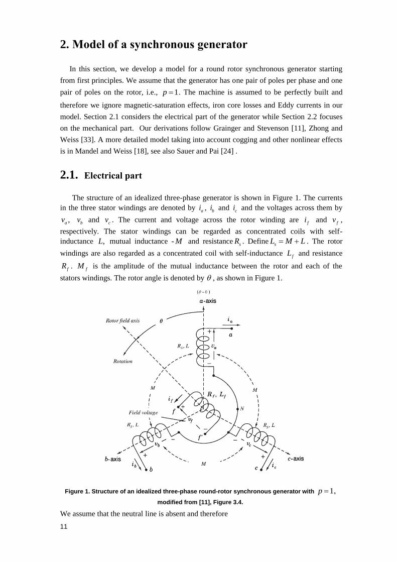
The structure of an idealized three-phase generator is shown in Figure 1. The currents
in the three stator windings are denoted by ai , bi and ci and the voltages across them by
,av bv and cv . The current and voltage across the rotor winding are fi and fv ,
respectively. The stator windings can be regarded as concentrated coils with self-
inductance ,L mutual inductance - M and resistance sR . Define sL M L . The rotor
windings are also regarded as a concentrated coil with self-inductance fL and resistance
fR . fM is the amplitude of the mutual inductance between the rotor and each of the
stators windings. The rotor angle is denoted by , as shown in Figure 1.
Figure 1. Structure of an idealized three-phase round-rotor synchronous generator with 1p ,
modified from [11], Figure 3.4.
We assume that the neutral line is absent and therefore

12
0.a b ci i i
Denote the stator fluxes by a , b and c . Define the vectors
, , ,
cos sin
cos cos 2 3 , sin sin 2 3 .
cos 4 3 sin 4 3
a a a
b b b
c c c
vi
i i v
i
v
v
The stator flux linkages are given by
os cs f fL i M i
and the rotor flux linkage f is given by
(2.1) ,c .osf f f fL i M i
The phase terminal voltage vector v satisfies
(2.2) d
, d
s s
iv e R i L
t
where T
a b ce e e e is the back EMF due to the rotor movement and it is given by
(2.3) d
sin cos ,d
f
f f f
ie M i M
t
where is the angular velocity of the rotor. e is also called the synchronous internal
voltage. Similarly, the field terminal voltage is
(2.4) f f f
fdv R i
dt
.
By applying the Park transformation
(2.5)
2π 2πcos cos cos
3 3
3 2π 2π( ) sin sin sin
2 3 3
1 1 1
2 2 2
U
to (2.2), we get the following expression:
(2.6) d
( ) ( ) ( ) ( )dt
s s
iL U R U i U e U v .
We denote ( )dqe U e , whose components are ,de qe and 0e (in this order). The vectors
dqv and dqi are defined similarly. It is easy to verify that

13
(2.7)
0
)d
0
(d
d q
q d
i idi
i id
i
U
which can be rewritten as
(2.8)
0
( )d
.d
0
d q
q d
i idi
i it d
i
Ut
Using this, we can rewrite (2.6) as follows:
(2.9)
0 0 0 0
d
d0
d q d d d
s q s d s q q q
i i i e v
L i L i R i e vt
i i e v
.
Since there is no neutral line, 0 0i and hence 0 0.e v From (2.9)
(2.10) d 1
d
d d d dq s
q q q qd s s
i i e vi R
i i e vit L L
.
Applying the Park transform to (2.3) we get
(2.11)
d d3 3
d d2 2
f fd f
f
qf f f
i ie M
Mt te
M i i
.
In (2.4), substituting for f from (2.1) and using the identity ,cos 3 / 2 di i (recall
that ( )dqi U i where ( )U is defined in (2.5)) it follows that
(2.12) .d d3
d 2 d
f df f f f f
i iL M R i v
t t
Using the equation for d
d
di
t from (2.9) in (2.12) we get
(2.13)
23 d 3 1 11
2 d,
2
f f f fsq d d f f
f s f s s f f
M i M RRi i v i v
L L t L L L L L
where 21 0 f f sM L L and 3.2 sL L By defining
(2.14)
123
, 12
f
f s
M
L L
3
2fm M ,
(2.13) can be written as
(2.15) d
.1
d
f fsq d d f f
f s s f f
i RRmi i v i v
t L L L L L

14
Now we obtain the following equation for di and qi from (2.10) by substituting for de and
qe from (2.11) and for d dfi t from (2.15):
(2.16)
1 d
.d
fsq d d f fd dq s
f s s f f
q qd s s
f
RRmi i v i vi ii R m
L L L L Li iit L L
i
2.2. Mechanical part
The energy stored in the machines magnetic field is
21 1 1 1
, , ,cos 2 2 2
.2
mag f f s f f f fE i i i L i M i i L i
The electromagnetic torque can be calculated as shown below (see [7], [10] and [11] for
details), where we use the relation mp , m is the mechanical rotor angle and 1p (as
explained at the beginning of this chapter):
(2.17) , constant, constant , constant ff f
mag mag mag
e
m m i ii i
E E ET p
cos 3, ,sin .
2f f f f f f q f qpM i i pM i i M i i mi i
Usually the mechanical torque is produced/regulated by a prime mover which often
consists of a turbine and a controller, see Chapter 9 in [16] for different types of prime
movers. In our model, we ignore the dynamics of the prime mover and instead assume that
the specified mechanical torque mT (plus the droop correction, explained below) acts on the
rotor. If we assume no cogging torque, which is the torque due to the interaction between
the permanent magnets or electromagnets of the rotor and the stator slots, then the
mechanical part of the machine is governed by
(2.18) ,m e pJ T T D
where J is the moment of inertia of all parts rotating, pD is the damping factor and the
rotation frequency is the first derivative of the rotor angle. The term pD is due in
part to viscous friction, but mostly it is due to the droop controller of the prime mover,
which adjusts the active torque depending on . The kinetic energy of the rotor is
2
kin 2E J . It follows that
.kin m e p m f q pE J T T D T mi i D
In the absence of any external torque ( 0mT ) and short circuit in all terminals, the change
in the total energy mag kinE E E of the system, must be equal to the loss of energy due to
mechanical damping (including the droop correction) and electrical resistance. It is easy to
check that

15
(2.19) 2 2 2 2- - 0.-mag kin s d q f f pE E E R i i R i D
This validates our energy calculations. Note that, if we neglect the viscous friction, then the
active torque acting on the generator is m pT D .
Using (2.15), (2.16), (2.17) and (2.18) we obtain the following system which models
the dynamics of a perfectly built synchronous generator with one pair of poles:
(2.20)
0
0d
0d
0 0
s fs d d
s s fs q q
s s ff f f
f p
Rs L mRL i i
L R miL i i
mR L m RL i it
mi DJ
0 0
0 1 0 0.
0 0
0 0 0 1
df
q
fs
m
vm L
v
vm L
T
We mention that this system can be represented as a port-hamiltonian system, see Fiaz, Zonetti, Ortega, Scherpen and van der Schaft [9].
3. Model of a synchronous generator connected to an
infinite bus
In this section we develop a model for a single synchronous generator (SG) connected to
the power grid. The grid is assumed to be an infinite bus, i.e., a constant three-phase AC
voltage source. This is a reasonable assumption since the influence of a single generator on
a grid consisting of many equivalent generators is typically small. To simplify the
presentation, the constants sL and sR are redefined to include the resistance and
inductance of the line leading to the bus. Thus the stator terminal voltage v is the voltage
of the bus. The bus voltage T
a b cv v v v depends on the bus angle bus as follows:
cos cos( cos2 3 , 2 3 2 3), 2 3 2 3)( .a bus busb sc buv V v V v V
Here 0 V is the line to line rms voltage. Define
2 ,bus
where is the rotor angle of the synchronous generator. This is the well-known power
angle, the angle by which the synchronous internal voltage e is ahead of the bus voltage v .
We apply the Park transform (2.5) to v . Using the definition ( )dqv U v , we get that
(3.1) sin , cosd qv V v V .
It is easy to see that
(3.2) g ,

16
where g is the constant bus frequency. Thus . From (2.17) and (2.18) we get
(3.3) p g f q mJ D mi i T .
If we can express qi as a (possibly approximate) function of , then from the above
equation an ODE in that resembles the classical swing equation can be obtained. We
will derive such an ODE using model reduction in Section 3.2.
We remember (2.20) for the dynamics of the full system. Now we add the state variable
with the state equation (3.2) and assign the values of dv and qv from (3.1) to get the
following ODE system with 5 state variables:
(3.4)
0 0
0 0d
0 0d
0 0 0
0 0 0 1 0
s d s f f d
s q s f q
f f s s f f
f p
L i Rs L mR L i
L i R mi i
L i mR L m R it
J mi D
sin0 0 0
cos0 1 0 0 0
.0 0 0
0 0 0 0
0 0 0 0 1
1
f
fs
m
g
Vm L
V
vm L
T
3.1. Linearization of the SG model on an infinite bus
We analyze the local stability of (3.4) by linearizing it near its equilibrium points in this
section. We assume that fi is constant (this assumption is made to simplify the
calculations). Then the nonlinear equations (3.4) reduce to
(3.5)
sin- 0 0
cos- - - 0d.
0 - 0d
-0 0 1 0
s d s s d
s q s s f q
mf p
g
VL i R L i
VL i L R mi i
TJ mi Dt
We compute the equilibrium points T
0 0 0 0d qi i for (3.5) by setting the derivatives of
all the state variables to be 0. Letting 0 , it follows from the fourth equation in (3.5)
that 0 g . The third equation in (3.5) (setting 0 ) gives
0 - 0f q p g mmi i D T
0
1.q m p g
f
i T Dmi
It follows from the second equation in (3.5) that
0 0 0sin 0 s d g s qR i L i V
17
0 0sin .g s
d m p g
s s f
LVi T D
R R mi
Finally we get from the first equation in (3.5) that
(3.6) 0 0 0 0co .sg s d s q f gL i R i mi V
We define Z and as follows: ,j
s g sZ R j L Z e so that
(3.7) 2 2 2 , arctan .s g s g s sZ R L L R
After substituting for 0di and 0qi in (3.6), using the definitions in (3.7), the power angle
at the equilibrium is given by the expression
(3.8)
0 arccos .m p gf g s
f
Z T Dmi R
Z V Vmi
This equation may have 0, 1 or 2 solutions modulo 2 . If there are two solutions, then
there are two equilibrium points and they are either both unstable or one stable and one
unstable. We want to linearize the system near a stable equilibrium point. For this we
compute the equilibrium points and check if any of them is stable. The linearized system
will be of the form
(3.9) .x Ax .
Define
0 00 0 ,, ,qd d qd qi ii i i i ,
where 0 0 0 0
T
eq d qx i i is an equilibrium point of (3.5), and denoteT[ ]d qx i i .
Define T
d qz i i and rewrite (3.5) in the form ( ),z f z then A in (3.9) is the
Jacobian defined by (
.)
eq
ii j
j z x
f zA
z
We calculate the Jacobian from (3.5) and get
0 0
0 0
cos
sin .
0 0
0 0 1 0
s s g q s
g s s d f s s
pfm
R L i V L
R L i mi L V LA
J D Ji
We need to assign parameter values to compute the equilibrium points of (3.5) and check if
they are stable, by computing the eigenvalues of the resulting Jacobian matrix. For the
nominal values of the parameters shown in Table 1, we obtain a pair of equilibrium points
0 0 0 0eq d qx i i shown below:
1 -6.7181 -12.2190 100 0.0398eqx , 2 -578.2614 -12.2190 100 -2.9624eqx .
For 1
eqx the matrix A is
34.5455 314.1593 12.2190
314.1593 34.54
90467
3602.555 289.3083
6.51
0 0
0 0 1
8
0
26 .5A

18
and the eigenvalues of A are:
1 2 3 4-34.88 + 314.23i, -34.88 - 314.23j, =-3.92 + 43j, =-3.92 - 43j .
For 2
eqx the matrix A is
34.5455 314.1593 12.2190
314.1593 34.
89089
161385455 282.3083
6.51
0 0
0 0 1 0
26 8.5A
and the eigenvalues of are:
1 2 3 4-34.87 + 314.22j, -34.87 - 314.22j, =-47.23, =39.38.
Notice that in both cases 1 and 2 are almost equal to .s s gR L j
Hence (3.5) has two equilibrium points, where 1
eqx is stable and 2
eqx is unstable. This is
true for typical values of the parameters. For some set of parameter vectors, it is possible to
show that the synchronous generator model (3.5) is almost globally asymptotically stable,
meaning that almost all the trajectories converge to the stable equilibrium point, see [20].
We remark that (3.4) can be linearized without the assumption of constant rotor current,
but the expressions become extremely complex and the model is very difficult to analyze.
In order to compare (3.5) to a reduced model that will be introduced in Section 3.2 we
will manipulate the linearized system x Ax , where T[ ]d qx i i and A is as
calculated above. We can write x Ax as a feedback interconnection of an integrator (with
input and output ) with the third order system
(3.10) 3 3 3 , ,z A z B z y C z
where T[ ]d qz i i and
0 0
3 0 3 0 3
cos
( ) , sin , 0 0 1 ,
0 0
s s g q s
g s s d f s s
f p
R L i V L
A R L i mi L B V L C
mi J D J
as shown in Figure 2.
Figure 2. The linearization of a synchronous generator
connected to an infinite bus, divided into two subsystems.
+ 𝜔𝑔
1
𝑠
𝛿
-

19
The transfer function of the third order system is
1
3 3 3 .G s C sI A B
The Bode and Nyquist plots for this transfer function, with 3 ,A 3B and 3C evaluated at
1 ,eqx are in Figure 3 and 4. The eigenvalues of 3A for
1
eqx are:
1 2 3-34.43 + 317.13j, -34.43 - 317.13j, =-8.74.
The eigenvalues of 3A for
2
eqx are:
1 2 3-34.92 + 311.25j, -34.92 - 311.25j, =-77.5.
In Section 3.3 we will derive a feedback interconnection, similar to that shown in Figure
2, but using a reduced model for the SG. We plot its Bode and Nyquist plots and compare
it with the plots in Figures 3 and 4. We do this comparison to ascertain the fidelity of the
reduced model.
Parameter Value
V - line to line rms value 230 3 398.37 V
5nP kW , gm gn pT P D 549.986 Nm
g 100π s−1
sR 0.152 Ω
sL 4.4 mH
fR 0.6 Ω
fL 0.3 H
fM 0.025 H
J (for 2 / 2 2secondsJ P ) 0.2 Kgm2
pD (100% increase of P for 3% decrease of ) 1.7 Js
fi 42.54 A
Table 1. Nominal values for a 5kW synchronous generator connected to a 50 Hz low voltage line in
a European or similar power grid.
The resulting parameters, , ,m and fmi at equilibrium are:
3.451, 0.0306H, 1.304Vs, 2 236.8f rms f fm mi e M i V V.
Some of the values in Table 1 are obtained from regulation requirements in Europe (for
instance the values of pD , J , g and )V . The values of sR and sL are selected to be the
same as those of the 5 kW synchronverter on which experiments are being conducted at Tel
Aviv University. The values of fR , fL and fM were chosen intuitively to match the other
parameters. The value of fmi was found via simulation of a simple system consisting of a
synchronous generator and an ideal voltage source. The Bode and Nyquist plots below
were obtained using standard MATLAB commands.

20
Figure 3. Bode diagram of the linearized subsystem described in (3.10) around the stable
equilibrium point1
eqx of the nonlinear model (3.5).
Figure 4. Nyquist diagram of the linearized subsystem described in (3.10) around the stable
equilibrium point 1
eqx of the nonlinear model (3.5).
3.2. The reduced order SG model
We develop a reduced order model for the fifth order system in (3.4). As mentioned
below (3.3), the idea is to express qi as a function of . Since sL is typically small,
following the singular perturbation theory (see Chapter 11 in [13]), we let / dd 0s d tL i
-150
-100
-50
0
50
Magnitude (
dB
)
100
102
104
106
-270
-180
-90
0
Phase (
deg)
Bode Diagram
Frequency (rad/s)
-50 0 50 100 150 200 250-150
-100
-50
0
50
100
150Nyquist Diagram
Real Axis
Imagin
ary
Axis

21
and / dd 0s q tL i in (3.4). In other words, di and qi are assumed to be fast variables. This
gives:
(3.11) sin
,fs
d q f f
s s f s f s
mRL V mi i i v
R R L R L R
(3.12) cos
.sq d f
s s s
L m Vi i i
R R R
We define the stator impedance ,s sZ R j L so that 2 2 2 .s sZ R L
Solving for qi from (3.11) and (3.12) gives
2
1cos sin .s
q f s s f f s s f
f f
m Lmi R L R L i V R L v
L LZ
Substituting for qi in (3.3) gives
p gJ D
2cos sin ,
f sm f s s f f s s f
f f
mi m LmT R L R L i V R L v
L LZ
which can be equivalently expressed as
(3.13)
p g mJ D T
2 2 2
2 2 2 2.cos sin
f s s fs s sf f f f
f f
R L R LVR V L Lmi m i m i v
Z Z Z L Z L
By definition sing sL Z and cossR Z ( Z and are defined before (3.7)). We
assume that g and therefore Z Z . By replacing Z with Z in (3.13) and
using the identity cos( ) cos cos sin sin and ,g we get:
(3.14)
2 2
2
2 2cos
f s s f fsp f f f
f f
m R L R L mi Vm LJ D i i v
ZZ L Z L
2 22
2 2.
f s s f sm p f f f g
f f
m R L R L m LT D i i v
Z L Z L
This ODE is coupled with another ODE that expresses fi , see (3.15) below.
From (3.4), the dynamics of fi is described by the equation
sind
d.
f fsd q f
f s f f f f s
f R vmR m mi i i V
L L L L Lt L
i
L
After substituting qi and di with their reduced model expressions (3.11) and (3.12), we get:

22
2 1 1 11 sin ,
f f
f f
f f s s f f f
di R m mi V v
dt L L L L L L L
which can be simplified to
(3.15) 1
.f f
f f
f f
di Ri v
dt L L
Irrespective of initial conditions, fi stabilizes to a final value that depends only on fv and
the values of the rotor parameters. The final value is
lim ( ) f f ft
ti v R
.
In other words the equilibrium value is 0 f f fi v R . Since we are interested in the long
time behavior of (3.14), we replace fi with 0fi and rewrite it as
(3.16) 2 2
2 2
2 22 2co .s
fs sp f m p f g
ff f
mv Vm R m RJ D v T D v
Z RZ R Z R
For the almost global stability of (3.16) it is necessary that
2
2
2 20,s
p f
f
m RD v
Z R
which holds trivially since both the terms on the left side are positive. For more information
on the stability of pendulum like equations, see [17]. To calculate the equilibrium points,
we let 0 and 0 in (3.16) and get the following expression for the equilibrium value
of :
0 arccos ,m p f f g s
f
g
f
T D Z R mv R
mVv V Z R
which is equivalent to (3.8) if we use f f fi v R . From here we get an additional
stability condition:
1 1.m p n f f g s
f f
T D Z R mv R
mVv V Z R
This condition appears to hold for most typical generator parameter values and in most
cases the system (3.16) has one stable equilibrium point.
In the above analysis we have made several assumptions, the most significant of them
being g . In the absence of this assumption, but still using the steady state value
f f fi v R , (3.16) had to be replaced with
(3.17) 2 2
2 2
2 22 2c ,os
fs sp f m p f g
ff f
mv Vm R m RJ D v T D v
R ZZ R Z R
where is the stator impedance angle, arctan s sL R .

23
The global stability of this system is an open question. But it is quite straightforward to
analyze the local stability of this system around an equilibrium point (the procedure for
local stability analysis was demonstrated in Section 3.1 for a more complex model). Future
work will focus on estimating the domain of attraction of the stable equilibrium point,
whenever it exists. Note that in this section the rotor current was not assumed to be
constant like it was in Section 3.1. However as seen from (3.15) the rotor current does not
depend on other state variables in the reduced model. Therefore in the stability analysis, the
rotor current can be regarded as a constant with value equal to its equilibrium value 0fi .
3.3. Linearization of the reduced order SG model
While analyzing the dynamics of a network of synchronous generators it is convenient
to use reduced order models. But it is not clear if the reduced models capture the primary
dynamics of the network. In Section 3.2 a reduced model (3.13), (3.15) was obtained for a
synchronous generator connected to an infinite bus. In this section we try to evaluate the
quality of this reduction. To do this we linearize the reduced model around a stable
equilibrium point and represent it as a feedback interconnection of a second order system
and an integrator (similar to that in Figure 2). We plot the Bode and Nyquist plots of the
second order system and compare it with the corresponding plots of the third order system
in Figure 2 so as to compare the reduced model to the full model with constant fi , (3.5). In
the reduced model fi is not assumed to be constant, but in the full model in Section 3.1 it
is assumed to be constant.
Define 0 0 0
T
eq fx i to be an equilibrium point of the reduced model (3.13), (3.15)
and define T
fz i . We calculate the Jacobian( )
eq
i
z
i
x
j
j
f zA
z
, where
2 2
2
cos sin( )
f f f f f
f s s f s f f s f f s f
m p
g
i R L v L
i mV R L m i R L R L i v L Lf y T D
Z
is defined using (3.15) , (3.2) and (3.13). We get that
21 22 0 0
0 0
sin( )
0 1 0
f f
f
R L
A A A mV i J Z
,
where
2 2
0 0 0
21 2
cos sin 2f s s g g f s f s f f s g
f
L mV R L v L m m i R L R LA
J Z L

24
2
0 0
22 4
2 cos
s g f s f
f
L mVL R iA
J Z L
2 2 2 2 2 2
0 0 0 0
4
( ) sin .
s g s f s f f s f f s f f s p
f
R L m i R L R L m i v L L i mVL D
JJ Z L
The equilibrium value of fi is ffv R and for we use (3.17) by letting 0 , 0
and substituting fv with 0f fi R to get :
0
0
0
arccos ,m p gf s g
f
Z T Di R m
V Z mVi
which is equivalent to (3.8). Again we have used the values from Table 1 and have
checked if there are equilibrium points. We have found two equilibrium points, where the
first point is 1 10042.54 0.0398T
eqx and the second is 2 42.54 100 -2.9624T
eqx .
We can use (3.11) and (3.12) to compute the values of di and qi according to 1
eqx and get
-6.7181di and -12.2190qi . We see that the values of di and qi along with and
have identical values to the values 0 0 0, ,d qi i and 0 in the stable equilibrium point 1
eqx
of the fourth order system (3.5). For the first equilibrium 1
eqx the matrix A is
2 0 0
7.08 8.9 517.6
0 1 0
A
,
and the eigenvalues are:
1 2 3-4.45 + 22.31j, -4.45 + 22.31j, =-2.
For the second equilibrium 2
eqx the matrix A is
2 0 0
7.08 7.614 517.6
0 1 0
A
and the eigenvalues are:
1 2 319.26, -26.87, =-2. We see that 1
eqx is the stable equilibrium, which
corresponds to the similarity in values.
Define T[ ]fx i , where 0 ,f f fi i i 0 and 0 . We examine
the linearized system x Ax , where T[ ]fx i and A is the 3x3 Jacobian matrix
calculated previously. We can write this system as a feedback interconnection of an
integrator (with input and out output ) with the second order system
(3.18) 2 2 2 , ,z A z B z y C z
where T[ ]fz i and

25
2 2 2
0 021 22
00 , , 0 1 ,
sin
f f
f
R LA B C
mVi JZA A
identical to what was done in Figure 2 and receive the following transfer function for the
second order plant:
2 2
1
2 .G C sI A Bs
We plot Bode and Nyquist diagrams using the values from Table 1 and get:
Figure 5. Bode diagram of the linearized subsystem described in (3.18) around the stable
equilibrium point 1
eqx of the nonlinear reduced model (3.13), (3.15). This should be compared to
Figure 3.
Figure 6. Nyquist diagram of the linearized subsystem described in (3.18) around the stable
equilibrium point 1
eqx of the nonlinear reduced model (3.13), (3.15). This should be compared with
Figure 4.
The reduced model is almost identical to the full model in the low frequency region.
This means that for the generator connected to the infinite bus, near an equilibrium point
we can use the model reduction to analyze the synchronous generator. In the future, we
hope to show that taking the rotor current to be constant (or slowly varying) is a good
approximation of the full fifth order system in (3.4).
0
10
20
30
40
50M
agnitude (
dB
)
10-1
100
101
102
103
-90
-45
0
Phase (
deg)
Bode Diagram
Frequency (rad/s)
-50 0 50 100 150 200 250-150
-100
-50
0
50
100
150Nyquist Diagram
Real Axis
Imagin
ary
Axis

26
4. Introduction to synchronverters
In this chapter we will use the model of the synchronous generator from Chapter 1 to
build the model of a synchronverter. The synchronverter is an inverter with a special
control algorithm that causes it to mimic the operation of a synchronous generator. We use
the same model of a synchronous machine as in Figure 1 with no neutral line connected.
(However we mention that synchronverters can be built also with a neutral line connected
to the grid.) Now we can take equations (2.2), (2.3), (2.4), (2.17) and (2.18) from Chapter 2
for our synchronverter model. We add an additional assumption of a constant rotor current
to simplify calculations. As mentioned in Section 3.3 this is not necessarily a good
approximation but it is required to simplify the design of the controller. If we consider the
synchronverter to be a small inverter (power wise) in a very large grid then the grid may be
regarded as an infinite bus, so that the equations of the system should be similar to (3.5).
Future work should include a comparison of these two models. We get the following
equations for our synchronverter:
(4.1) ,s s
div R i L e
dt
(4.2) sin ,f fe M i
(4.3) , i ,s ne f f iT M i
(4.4) ,m e pJ T T D
.
The active and reactive power are defined by , P i e and , quadQ i e , where
cos .quad f fe M i We can calculate the active power and the reactive power using the
simple equations:
,sin ,f fP M i i
(4.5) ,cos .f fQ M i i
These equations give us the basic algorithm of the synchronverter shown in Figure 7:

27
Figure 7. Electronic part of a synchronverter (without control), typically running on a DSP.
Note that, if we assume no viscous friction, then the virtual active torque acting on the
rotor is .m pT D The fact that this expression depends on means that it is actually a
feedback loop, called frequency droop. As was mentioned in Section 2.2 (about the model
of the synchronous generator), we consider the torque mT to be constant or an input which
changes by user demand. To avoid sharp transients, we add an LPF for the signal .mT If we
denote ,n m p nT T D which is the active torque at the nominal frequency n , then
.m n p nT T D
Since the frequency of the synchronverter follows the frequency of the grid, the
synchronverter will change its output power so that for frequencies above nominal the
power will be less then the nominal power, while for frequencies below nominal, the power
will be more than the nominal power. We would like to choose the droop coefficient pD so
that it matches the real droop coefficients used in synchronous generators. For example for
most generators in the European grid, for a 3% change in frequency the power will change
100% from nominal. Obviously for a real system this cannot always be obtained. We don't
always have enough energy stored or the ability to absorb energy in our system. Later on
we will show how to handle this problem.
The importance of J should also be noted. J should receive a value that allows the
machine to have an inertia time constant that fits an actual synchronous generator. For the
synchronverter we prefer the lowest of values of J , since it slows down system response
time and may cause stability problems. Let H be the inertia time constant of a
synchronous generator, defined as 21
.2
n nH J P It is known that: 2sec 12sec.H
This leads to 24 n nJ P and 2 droop rate ,p n nD P where the droop rate is the
proportion of n that will cause a 100% change in mT (typically around 0.03).
For voltage and reactive power control an additional control loop is required. The rotor
current is considered constant or at least slowly changing, and as we have seen the rotor
flux has a strong influence on the voltage amplitude in the synchronous generator, see
Eqn (4.2) Eqn (4.3)
Eqn (4.5)

28
(4.2). Indeed, the synchronous internal voltage e is the most significant component in the
voltage v from (4.1) since we can assume small resistance and inductance of the stator.
We use the approximate relation
(4.6) 2
3 cos VE V
QX X
derived in [16], where V is the rms voltage value on one phase of the synchronverter
terminals, E is the rms value of e , is the power angle as defined in (3.1) and sX L
is the absolute value of the stator impedance when sR is neglected. We see from (4.2) that
we can use the rotor flux to control E and so also the reactive power using a simple
integral controller. We can see this also directly from (4.5). We want to enable a change in
Q using a change of rotor flux with minimum changes to P, which we have already
controlled using the frequency droop part. Most synchronous generators operate in a PV
(power-voltage) control scheme. This means that the generator will help stabilize voltage
by supplying or absorbing reactive power. For this we add another droop loop for voltage
dependent reactive power
0.setq
n
Q Q QD
V V V
Here Q is the output reactive power, setQ is the desired reactive power for nominal
voltage, V is the measured rms voltage on the synchronverters terminals and nV is the
nominal rms voltage. The integrator on the rotor flux control loop (shown in Figure 8) has a
gain1 0K . Choosing K and qD depends on the application, by tuning. Larger K means
a slower system but usually more stable. Larger qD means that the synchronverter will try
harder correcting the voltages at the expense of accurately tracking the desired setQ . In
order to work in a PQ (power-reactive power) control scheme, only reactive power control,
the user can take 0qD . Measuring the amplitude of the voltage on the synchronverter
terminals requires extra work in the algorithm. Here we make the assumptions that the
system is symmetric, balanced and has no higher harmonics. Under these assumptions the
voltage amplitude detection is very simple (see [33] for more information):
(4.7) 2 3 ,g a b b c c aV v v v v v v
where ,a bv v and cv are the measured voltages on the synchronverters terminals. In
software implementation one should check that the sum inside the square root is indeed
positive to avoid Nan (not a number) errors. Since this expression doesn’t always hold, if
the grid is unbalanced, it is recommended to pass the measured voltages through an LPF.
The same is true for Q and ,eT see Figure 8. This LPF is a tunable filter, my chosen values
for simulations will be discussed in Section 12. The initial condition for the rotor flux
should be the approximate steady state value which can be calculated from
(4.8) f f nM i e ,

29
where e is the expected amplitude of e from (2.3) (about 10% higher than the amplitude
of the nominal grid voltage).
Synchronization of the synchronverter to the grid can be done by using a PLL, but there
is a better way. The paper [32] presents the design of a self-synchronizing synchronverter.
This is implemented by adding 3 software implemented switches. The first switch, QS turns
off the voltage control part, qD . The second switch CS connects a virtual resistor and
inductor virR and virL , where a virtual current is calculated from measured grid voltage,
instead of a measured current. This is done since without synchronization we can't connect
the synchronverter to the grid, to avoid a large current and a large transient at the moment
of grid connection. In our equations, see (4.3) and (4.4) we see that the measured current
plays an important role. This means we must find a suitable replacement. Usually we select
the virtual resistor to be twice the stator resistor and the virtual inductor is identical in size
to the actual inductor. The calculation of the current is as follows:
vir
ˆ ˆ( ) ( )ˆ ( ) ,
g
vir vir
e s v si
L s Rs
where a denotes the Laplace transform, s is the complex variable, e is the internal
synchronous voltage vector, gv is the measured grid voltage vector and viri is a vector
replacing i . The third and last switch PS connects a PI controller to the frequency droop
loop in order to replace the nominal frequency of the grid, which is 50Hz for Europe and
60Hz in North America, with the actual grid frequency g estimated via r . This
calculation is required because the grid frequency may deviate from nominal values by a
small portion. During the entire synchronization process setP and setQ are set to be 0. The
purpose is to make the synchronverter create a mirror image of the grid where no power is
delivered to or from the grid. The result is a smooth connection to the grid and afterwards
we can slowly increase setP and setQ . It is recommended to give different values for the
synchronverter constants when synchronizing. Smaller inertia constant will significantly
reduce the synchronization time. Increasing the integrator constant K in the reactive
power control loop will slow synchronization but will help stabilize the process.
Choosing these new values must be done carefully since the system can become
unstable! For instance, if g virL is small compared to virR and if K is relatively small, then
the system will oscillate.

30
Figure 8. Proposed controller (electronic part) for a self-synchronized synchronverter, following
[32].
Finally we mention briefly the PWM (Pulse Width Modulation, see [8]) part and the
filters that connect the inverter to the grid. The desired signal e computed by (4.2) is sent
to a PWM signal generator that opens and closes electronic switches (IGBT or MOSFET,
see [14]) in order to generate an approximation of a sine wave in the low frequency range.
The switching frequency must satisfy two conditions. We want the switching frequency to
be high enough so that the Total Harmonic Distortion (THD) will be sufficiently low, the
exact value depends on regulations and application. We want our filter resonant frequency
to be at least five times lower than the switching frequency, so that switching noises won't
be increased due to resonance. As an upper bound we want to minimize our losses on the
switches which we know increase with frequency. A switching frequency of 10 kHz is
good enough for a 5 kW inverter that was tested in our simulations and later on in the lab.
Before giving a detailed description of the PWM system used, we will give a short
background on three phase inverter topology. The topology shown below in Figure 9 is
based on the model of the canonical switching cell, see [22] and it is used for most power
converters. This allows a two way power flow.

31
Figure 9. Scheme of a 2-level 3 phase inverter with neutral line based on the model of the basic
switching cell.
The figure also shows a neutral line. In our simulations that line was not included. In order
to reduce losses and noise we have improved the switches for each phase and implemented
a neutral point clamped inverter topology with three DC voltage levels (the neutral is
represented as ground):
Figure 10. Neutral clamped inverter topology for one phase of a 3-level, 3 phase inverter.
On each phase there is a fast switch between neutral and V when the desired sine wave e
is positive, and between neutral and V when e is negative. Usually the voltages are
symmetric, meaning that V V , to generate a symmetric sine wave around 0. The circuit
in Figure 10 is operated as follows:
1 PV V S and 2 S are closed,
20 PV S and 3 S are closed,
3 PV V S and 4 S are closed.
The filter used to connect the inverter to the grid is an LCL filter. This is a very well-
known filter used in many inverters. This filter also has the role of being similar to the
stator , s sR L if we neglect the capacitor (which is needed to reduce the ripple).

32
Figure 11. Schematic of a 2-level 3 phase inverter connected to the grid via an LCL filter and a
circuit breaker.
The LCL filter is mainly meant to reduce harmonics and make the output current smoother.
There are a few basic rules for selecting the filters capacitor and inductors. We want less
than 5% current ripple, less than 10% voltage drop on the inductors and a resonance
frequency of about 20 times more than the grid frequency 50 Hz. This will allow second
and third harmonics to pass but higher harmonics, which include harmonics caused by the
switching, will be blocked. The formulas for gL and C below were calculated by a basic
calculation of the ripple of the current and voltage drop on both inductors, the formula for
sL is taken from the model of the basic switching cell:
2Δ , s sL V T i g n n sLL i LV and 2 1 || 20 .g s nC L L
Here i is the current ripple, LV is the voltage on the two inductors, sT is the switching
period and n is the nominal frequency. The last formula insures that the resonant
frequency of the LCL filter is around 20 .n Typically LV is 5% - 10% of nV (the nominal
rms phase voltage). Once the filter values , ,s gL L C are calculated for an inverter that
transfers power 1P , the filter values 2 2 2, ,s gL L C for another inverter that transfers power
2P , with identical ripple characteristics and switching frequency, are given by:
1 22 122 , s s g gL L PP L L P P and 22 1C C P P .
Since simulations with the exact switching model take a very long time to run, it is
desirable to replace the switching model with an average model average model that
contains a controlled voltage source instead of switches. To validate this replacement, we
have run simulations of a synchronverter with the switches and with the average model. In
the simulations we have used a self-synchronized synchronverter with the nominal power
5kW connected to an infinite bus. The solver used was ode23tb, which was recommended
when working with SimPower elements. We let 3.5kWsetP and 500VArsetQ . The
voltage was 404.158 V line to line rms. Figures 12 and 13 show the active power and
reactive power profiles from the two simulations:

33
Figure 14 shows the frequency from the two simulations:
Figure 12. Active power profile of a synchronverter connected to an infinite bus simulated with
PWM and with an average model using a controlled voltage source.
Figure 14. Frequency of a synchronverter connected to an infinite bus simulated with PWM and
with an average model using a controlled voltage source.
Figure 13. Reactive power profile of a synchronverter connected to an infinite bus simulated
with PWM and with an average model using a controlled voltage source.

34
5. Additional improvements to the synchronverter
algorithm
Chapter 4 presented the background on synchronverters, mainly based on [32] and [33].
In this chapter we propose several improvements for the synchronverter model. As
mentioned earlier the power supplied by any real source cannot change instantaneously. In
order to prevent the inverter from requiring the battery or PV array to change their outputs
instantaneously, we filter setP and setQ with LPFs before further processing. The filter
bandwidth has been chosen to be 4 rad/s.
Another practical problem arises when the frequency deviation from the nominal value
is large and the power that the synchronverter is required to supply or absorb is more than
physically possible. To solve this problem we divide the frequency droop loop into two
branches: a high and a low pass branch. All the torques except the torque from the high
pass branch and eT are saturated (see Figure 15) thereby limiting the power requirements.
We chose 20 rad/sec to be the cutoff frequency for the filter in the low branch of the
frequency droop loop.
The final change made to the algorithm is the addition of an over current protection
before the PWM. We estimate the current by first computing the vector e v (the notation
is as in (2.2) so that v is now the voltage vector on the filter capacitor). In order to
calculate the current i , we also need to estimate the impedance of the inductor nearest to
the switches. We assume that the frequency is almost the same as the nominal grid
frequency and compute the inductor impedance Z using (3.7). It follows that
.e v Z i From here we get that the maximal voltage difference e v allowed,
based on the maximal current allowed to pass through the inverter using
max max.e v Z i Using a saturation block, we ensure that e v Z i component-
wise. This does not replace the usual overcurrent protections for the inverter, but it can give
an additional layer of protection provided that the current can be saturated without
distorting the signal significantly and that our assumption of the frequency, i.e., it is near
nominal grid frequency, is correct.
All these new changes give us the updated synchronverter scheme shown in Figure 15.

35
Figure 15. Updated scheme of the synchronverter algorithm including filters on setP and setQ ,
saturation of output power and extra protection from high currents.
Another possible change to the synchronverter structure is an additional LPF before the
saturation block of the torque loop. This LPF can simulate the delay caused by additional
mechanisms such as an MPPT (controller that tracks the most efficient voltage to be acting
on a PV cell for maximum power generation) for a PV array (due to the fact that the
DC/DC transformer that delivers power to the inverter is delayed by the MPPT control in
case additional power from a storage unit is also required) or a DC/DC transformer that is
supposed to discharge an energy storage unit, such as a battery or super capacitor. This LPF
should be conditioned to work only if the required output power is greater than the power
available nominally to the synchronverter. This is because we will not need to discharge
energy from a storage unit if the required power is smaller to or equal to the power
generated nominally by the energy source, usually a PV array.

36
6. Some simulation results for synchronverters
In this chapter we will show that the synchronverter works like a synchronous generator
in a simple grid containing either another synchronverter or an infinite power source
(infinite bus) with a transformer of ratio 1:1 and loads modeled as power sinks equal to
more or less the nominal power of the synchronverter. This will be done by simulations in
Matlab using the average model of a synchronverter designed for 5kW nominal output
power. We will show 4 scenarios. The first 3 consider a single synchronverter and a grid
with loads and a transformer of ratio 1:1 as described above with an additional line
impedance of 1 mΩ and 2 mH between the infinite bus and the loads. The last one
considers a grid composed of 2 synchronverters, where the first generates the grid by
working in island mode with constant voltage and frequency references and the second
synchronverter synchronizes and joins.
In the first scenario we connect the synchronverter to an infinite bus and slowly decrease
the bus frequency at the rate of 1Hz per second until it reaches 48 Hz. We would like to see
that the synchronverter tracks the grid frequency and maintains a power-frequency droop of
100% power increase per 3% frequency decrease. We would also like to see that the power
does not exceed a maximum of 8kW. The active power of the synchronverter will be set to
3kW, while its nominal power is 5kW. So when the grids frequency decreases to 48.5Hz
synchronverter should reach 8kW and saturate.
Figure 16. The synchronverter connects to the infinite bus at t=0.14s. The grid frequency starts
decreasing at t=2s at a rate of 1 Hz per second until it reaches 48 Hz at t=6s. At t= 7s the grid
frequency starts climbing back to its nominal value at a rate of 1 Hz per second. We see that the
synchronverter tracks the grid frequency changes.

37
Figure 17. The synchronverter connects to the infinite bus at t=0.14s. The active power stabilizes
to 𝑷𝒔𝒆𝒕 = 𝟑𝒌𝑾. When the grid frequency starts decreasing at t = 2s, the synchronverter starts
increasing its power until reaching saturation at t=5.5s, while the grid frequency goes down to
48.5 Hz. The grid frequency starts increasing to its nominal value at t = 8s and shortly afterwards
the synchronverter starts decreasing power back to its nominal value.
In the second scenario a synchronverter is connected to an infinite bus and we slowly
increase the bus frequency at the rate of 1Hz per second until it reaches 52 Hz. We would
like to see that the synchronverter tracks the grid frequency and maintains a power-
frequency droop of 100% power decrease per 3% frequency increase. We would also like
to see that the power does not go below the minimum of 0kW. The active power of the
synchronverter will be set to 3kW and the nominal power is 5kW. So when the grids
frequency increases to 51.5Hz synchronverter should reach 0kW and saturate.
Figure 18. The synchronverter connects to the infinite bus at t=0.14s. The grid frequency starts
increasing at t=2s at a rate of 1 Hz per second until it reaches 52 Hz at t=6s. At t=7s the grid
frequency starts falling back to its nominal value again at a rate of 1 Hz per second. We see that the
synchronverter tracks the grid frequency changes.
38
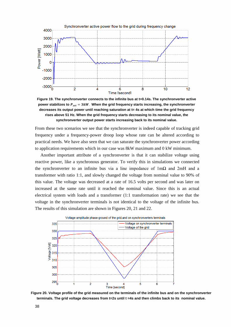
Figure 19. The synchronverter connects to the infinite bus at t=0.14s. The synchronverter active
power stabilizes to 𝑷𝒔𝒆𝒕 = 𝟑𝒌𝑾. When the grid frequency starts increasing, the synchronverter
decreases its output power until reaching saturation at t= 4s at which time the grid frequency
rises above 51 Hz. When the grid frequency starts decreasing to its nominal value, the
synchronverter output power starts increasing back to its nominal value.
From these two scenarios we see that the synchronverter is indeed capable of tracking grid
frequency under a frequency-power droop loop whose rate can be altered according to
practical needs. We have also seen that we can saturate the synchronverter power according
to application requirements which in our case was 8kW maximum and 0 kW minimum.
Another important attribute of a synchronverter is that it can stabilize voltage using
reactive power, like a synchronous generator. To verify this in simulations we connected
the synchronverter to an infinite bus via a line impedance of 1mΩ and 2mH and a
transformer with ratio 1:1, and slowly changed the voltage from nominal value to 90% of
this value. The voltage was decreased at a rate of 16.5 volts per second and was later on
increased at the same rate until it reached the nominal value. Since this is an actual
electrical system with loads and a transformer (1:1 transformation rate) we see that the
voltage in the synchronverter terminals is not identical to the voltage of the infinite bus.
The results of this simulation are shown in Figures 20, 21 and 22.
Figure 20. Voltage profile of the grid measured on the terminals of the infinite bus and on the synchronverter
terminals. The grid voltage decreases from t=2s until t =4s and then climbs back to its nominal value.

39
Figure 21. In the same experiment as in Figure 20, the synchronverter connects to the grid at
t=0.14s and its frequency remains constant when the voltage changes.
We see in Figure 20 that the synchronverter is able to slightly improve the voltage drop (the
voltage on the synchronverter terminals drops to 305 Volt and not 300 Volt). This is
achieved without changing the frequency (as seen in Figure 21) by producing reactive
power.
Figure 22. The reactive power of the synchronverter stabilizes at its nominal value at t = 2s. It then
increases because grid voltage drops. After t = 4s the reactive power decreases because the grid
voltage climbs back to its nominal value. The nominal reactive power of the synchronverter was
set to 500 VAr, but the synchronverter does not stabilize at 500 VAr due to the voltage drop on the
line impedance.
It is important to note that the behavior shown in Figures 20, 21 and 22 is not a Fault Ride
Through. A Fault Ride Through mechanism means changing the algorithm to make sure
certain regulations are met. Since this algorithm was not designed for a specific regulation
such a mechanism was not designed. A simple check is done to detect voltage drops (will
be discussed in Section 12.1) and short circuits. It is left for future designers of the
synchronverter to decide what to do when such a fault occurs. For now only the most basic
regulation is kept, i.e. the synchronverter disconnects after a fault of more than 30
milliseconds with the terminal voltage amplitude under 30% of the nominal value, or if the

40
frequency change rate exeeds 8 Hz per second. An additional check for correct frequency
range is also done routinely in the algorithm to make sure synchronverter frequencies are
not above or below allowed grid frequencies. As we see it is very easy to fit the
synchronverter algorithm to any given regulation. This simplicity is very important in the
fast changing world of renewables and smart grid applications.
Next we will investigate a micro grid (in simulations) composed of two synchronverters
and two loads. We expect that this grid behaves like an interconnection of 2 synchronous
generators. To test this we perform some load changes and track the frequencies at which
the micro grid stabilizes. We have designed this experiment so that the frequency will be
around 50 Hz. We choose a non-symmetric system in which the synchronverter that starts
the micro grid, called the grid synchronverter, is working slightly above full capacity, i.e. it
is designed to supply 5kW at the nominal frequency 50 Hz, but it supplies 5.5kW to the
two loads and so cannot work at the nominal frequency. The first load closest to the grid
synchronverter is 4kW and the second is 1.5kW. Between the two loads there is a small
impedance with resistance 1 mΩ and inductance 2mH. Figure 23 below describes this
system.
Figure 23. The two synchronverter micro grid. The fisrt synchronverter with 𝑷𝒔𝒆𝒕 = 𝟓𝒌𝑾 starts the
micro grid. The second synchronvertert connects after 4 seconds. The 1 kW load is connected at t
= 9s, 5 seconds after the second synchronverter connects to the micro grid.
After 4 seconds we allow the second synchronverter to connect to the micro grid and see
that indeed the micro grid frequency rises slightly above 50 Hz (see Figure 25) and the
loads are shared between both synchronverters as expected. The first synchronverter has an
active power of 4.5kW while the output of the second is 1kW, see Figure 24. Another 5
seconds later we add an additional load of 1kW and this causes the grid frequency to drop
and the extra load is shared between the two synchronverters. This additional load causes
the demand for power in the micro grid to be equal to the sum of the nominal power of the
grid synchronverter (5kW) and the second synchronverter (1.5kW). This causes the system
frequency to stabilize to its nominal value 50 Hz. Both synchronverters have identical
parameters except their active power set points. Both synchronverters were set to output
500 VAr.
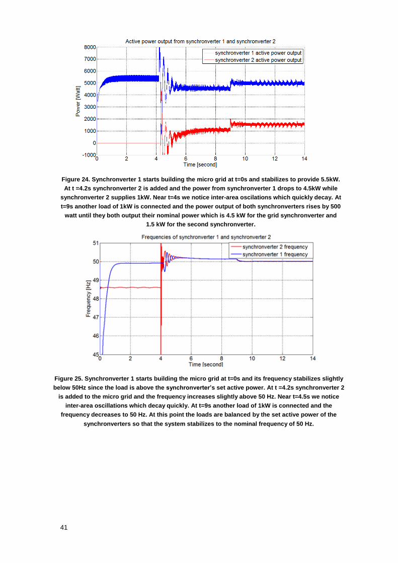
41
Figure 24. Synchronverter 1 starts building the micro grid at t=0s and stabilizes to provide 5.5kW.
At t =4.2s synchronverter 2 is added and the power from synchronverter 1 drops to 4.5kW while
synchronverter 2 supplies 1kW. Near t=4s we notice inter-area oscilations which quickly decay. At
t=9s another load of 1kW is connected and the power output of both synchronverters rises by 500
watt until they both output their nominal power which is 4.5 kW for the grid synchronverter and
1.5 kW for the second synchronverter.
Figure 25. Synchronverter 1 starts building the micro grid at t=0s and its frequency stabilizes slightly
below 50Hz since the load is above the synchronverter’s set active power. At t =4.2s synchronverter 2
is added to the micro grid and the frequency increases slightly above 50 Hz. Near t=4.5s we notice
inter-area oscillations which decay quickly. At t=9s another load of 1kW is connected and the
frequency decreases to 50 Hz. At this point the loads are balanced by the set active power of the
synchronverters so that the system stabilizes to the nominal frequency of 50 Hz.

42
7. Inter-area oscillations
We hope that the synchronverter can be used to solve practical problems in an actual
power grid. To verify this we need to consider specific problems, the current approach to
solve them and then propose new solutions using the synchronverter. We have chosen to
focus on inter-area oscillations. We will explain what they are and how they are dealt with
today. Finally we will present our solution to inter-area oscillations using synchronverters.
Local oscillations are associated with a single generator, due to its dynamics vaguely
resembling the dynamics of a damped pendulum (the swing equation). The frequency range
of these damped oscillations is approximately 0.7 to 2 Hz. In contrast inter-area oscillations
involve groups of generators which oscillate against one another when the physical link
between them is weak (i.e., it has relatively high impedance), see [15] for details. These
oscillations are much more complex since they involve several non-linear systems. The
oscillation frequencies range from 0.1 Hz to 0.8 Hz. A key feature of these oscillations is
that the power variations in one (group of) generator will be opposite to the power
variations in the other (group of) generator.
Inter-area oscillations are caused by the electro-mechanical nature of the generators.
They constitute a well-known problem, see for instance [16], [15], [21] and [29], and the
usual solution is to regulate the field voltage with a controller called Power System
Stabilizer (PSS). This requires additional hardware and each type of PSS has its own pros
and cons. Designing a PSS controller is a hard task which requires comprehensive
knowledge of the system, including all modes of oscillations involved, and careful thinking
about which of the several generators should have a PSS installed.
We explore inter-area oscillations by simulation experiments: we look at a simple grid
composed of two synchronous machines of 1 GW nominal power, each using a steam
Figure 26. Synchronverter 1 starts building the micro grid at t=0s. Its terminal voltage stabilizes
slightly below the nominal value of 330 V (amplitude). At t=4.2s synchronverter 2 is connected
and the voltage starts fluctuating, it increases until t=9s when another load of 1kW is
connected.
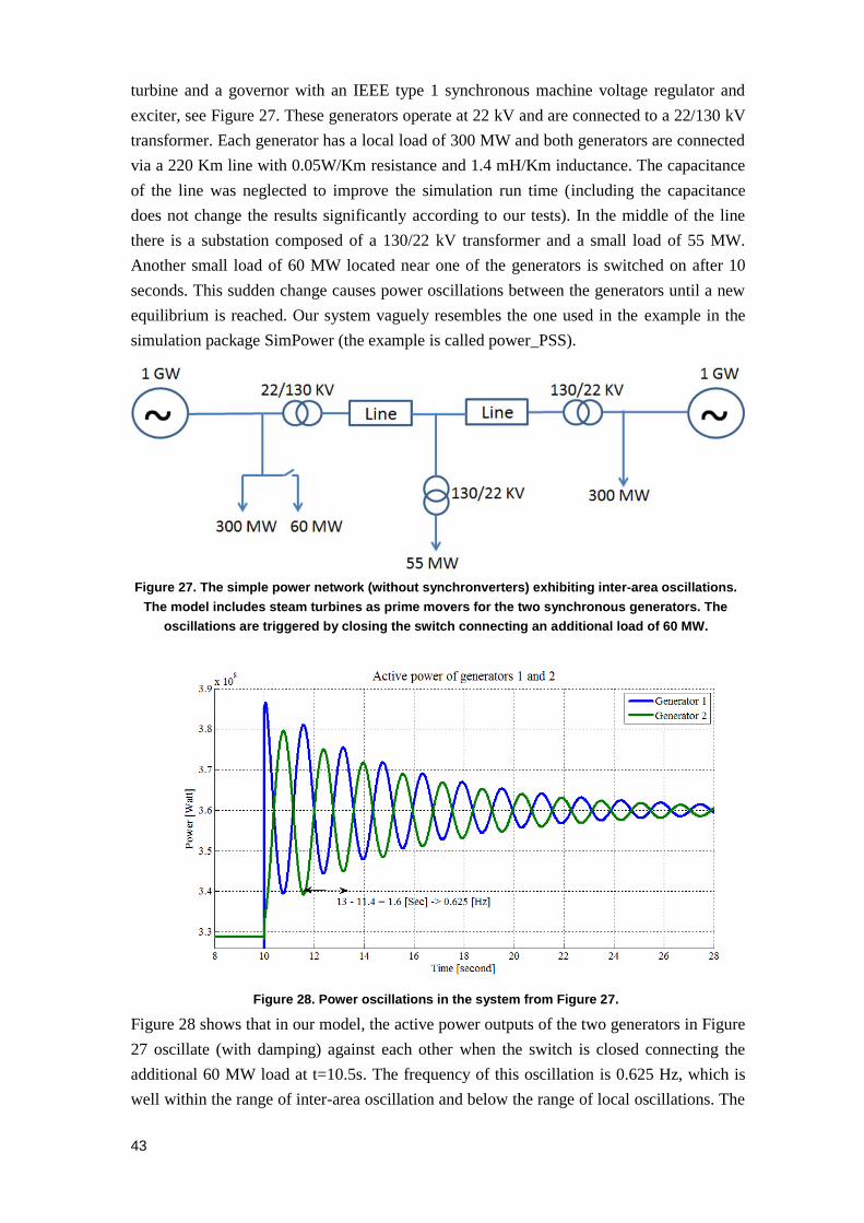
43
turbine and a governor with an IEEE type 1 synchronous machine voltage regulator and
exciter, see Figure 27. These generators operate at 22 kV and are connected to a 22/130 kV
transformer. Each generator has a local load of 300 MW and both generators are connected
via a 220 Km line with 0.05W/Km resistance and 1.4 mH/Km inductance. The capacitance
of the line was neglected to improve the simulation run time (including the capacitance
does not change the results significantly according to our tests). In the middle of the line
there is a substation composed of a 130/22 kV transformer and a small load of 55 MW.
Another small load of 60 MW located near one of the generators is switched on after 10
seconds. This sudden change causes power oscillations between the generators until a new
equilibrium is reached. Our system vaguely resembles the one used in the example in the
simulation package SimPower (the example is called power_PSS).
Figure 27. The simple power network (without synchronverters) exhibiting inter-area oscillations.
The model includes steam turbines as prime movers for the two synchronous generators. The
oscillations are triggered by closing the switch connecting an additional load of 60 MW.
Figure 28. Power oscillations in the system from Figure 27.
Figure 28 shows that in our model, the active power outputs of the two generators in Figure
27 oscillate (with damping) against each other when the switch is closed connecting the
additional 60 MW load at t=10.5s. The frequency of this oscillation is 0.625 Hz, which is
well within the range of inter-area oscillation and below the range of local oscillations. The

44
system was stable before the load jump and no power was transferred from one generator to
the other. The oscillations last for more than 20 seconds and even after 10 seconds they
have an amplitude of 10 MW which can cause heating in the lines and transformers.
7.1. Power system stabilizers
There are solutions to the problem of inter-area oscillations, as we stated earlier, but
they are far from perfect and require changes to the generators themselves. The most
common solution is the PSS which we will now review. The excitation control system in a
conventional SG controls the rotor current fi and its main purpose is to make sure that the
generator maintains a terminal voltage close to the nominal voltage. The reactive power of
a generator is closely related to the terminal voltage: in sinusoidal steady state,
2
3 cosVE V
QX X
where V and E are rms values as in equation (4.6). This
expression is fundamental in the field of AC power systems, for more information see [16].
The excitation control system provides the direct current to the field winding which in turn
determines the voltage of the generator and the reactive power. If we look at the formula
for the active power, which in steady state is 3
sin , VE
PX
(E, X, V and have the
same values as in equation (4.6)) we see that P depends on the voltages V and E. However,
since the variations in V and E are small, P is mainly changed via (which changes as a
result of changes in the active torque of the prime mover). Power System Stabilizers (PSS)
use the dependence of P on E to dampen inter-area oscillations as well as local oscillations,
see for instance [16], [30]. The general structure of a PSS shown below is taken from [30]:
Figure 29. General model of a PSS.
We have demonstrated the efficiency of various PSS by adding them to our simulation
model from Figure 27. We have used 3 types of PSS available in the Matlab SimPower
library. The first is called Multi Band PSS (MB PSS) and the input to it is the rotor angle
velocity deviation from nominal frequency. It handles 3 bands of frequencies (low,
intermediate and high) adjusted in advance. The second is a generic PSS the input to which
is the rotor speed deviation (from nominal frequency) multiplied with a constant gain and
filtered, as shown in Figure 29. The last PSS is almost like the second, but works on the
difference between electrical and mechanical power instead of rotor angle velocity
deviation.

45
Figure 30. Comparison of power oscillations using three types of PSS, as well as no PSS, in the
system from Figure 27.
We can see that the various PSS perform well, but have certain disadvantages. MB PSS is
the best of those tested here but it requires very precise design based on an accurate model
of the system. The second PSS (also called dω PSS) takes a long time to reach the new
equilibrium point. Even after 20 seconds it is far from settled. The third type of PSS
(also called m eP P PSS) causes large and very low frequency power oscillations. All three
PSS have the disadvantage of having an adverse effect on voltage regulation since they
work by changing the field current and hence E. Maintaining a constant voltage is
important for transformers and certain loads. After presenting our solution to the inter-area
oscillation problem, we will show the voltage profile of the various PSS.
7.2. Synchronverters with virtual friction
7.2.1 Frequency droop based solution
We would like to solve the problem of inter-area oscillations by using the
synchronverter which is an available resource rather than modifying the generators by
adding a PSS unit. Adding a PSS unit to a synchronous generator is not a simple process. It
requires identifying the generator on which the extra controller must be added. This means
deciding which is the most important generator from a power stand point and from a
voltage regulation stand point since PSS damages voltage control.
From (4.4) we see that the droop factor pD plays a main role in the damping of
frequency oscillations in the synchronverter. The frequency droop loop in the
synchronverter is fast since it has no mechanical parts, only electronic components. This is
unlike a real generator in which the droop loop acts on the prime mover and therefore has
delays due to physical limitations (of the order of one minute). This means that generators
are more sensitive to oscillations and adding our synchronverter to the grid, even without
any changes, can potentially improve system behavior.
To study the above idea, two synchronverters were added to the small grid from Figure
27, one near each generator, using transformers (inverters do not work at high voltages due
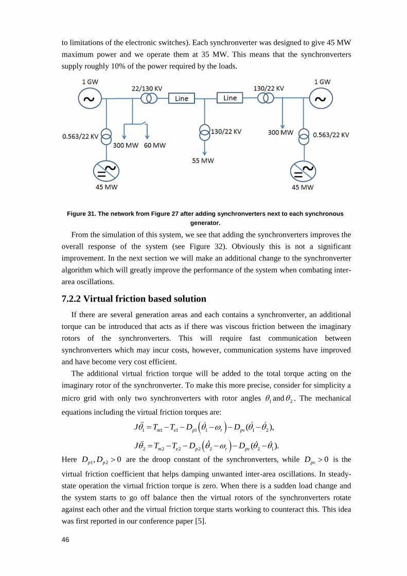
46
to limitations of the electronic switches). Each synchronverter was designed to give 45 MW
maximum power and we operate them at 35 MW. This means that the synchronverters
supply roughly 10% of the power required by the loads.
Figure 31. The network from Figure 27 after adding synchronverters next to each synchronous
generator.
From the simulation of this system, we see that adding the synchronverters improves the
overall response of the system (see Figure 32). Obviously this is not a significant
improvement. In the next section we will make an additional change to the synchronverter
algorithm which will greatly improve the performance of the system when combating inter-
area oscillations.
7.2.2 Virtual friction based solution
If there are several generation areas and each contains a synchronverter, an additional
torque can be introduced that acts as if there was viscous friction between the imaginary
rotors of the synchronverters. This will require fast communication between
synchronverters which may incur costs, however, communication systems have improved
and have become very cost efficient.
The additional virtual friction torque will be added to the total torque acting on the
imaginary rotor of the synchronverter. To make this more precise, consider for simplicity a
micro grid with only two synchronverters with rotor angles 1 and 2 . The mechanical
equations including the virtual friction torques are:
1 1 1 1 1 1 2( ),m e p r pvJ T T D D
2 2 2 2 2 2 1( ).m e p r pvJ T T D D
Here 21 0,p pDD are the droop constant of the synchronverters, while 0pvD is the
virtual friction coefficient that helps damping unwanted inter-area oscillations. In steady-
state operation the virtual friction torque is zero. When there is a sudden load change and
the system starts to go off balance then the virtual rotors of the synchronverters rotate
against each other and the virtual friction torque starts working to counteract this. This idea
was first reported in our conference paper [5].
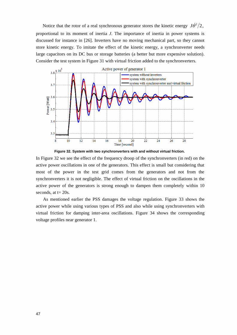
47
Notice that the rotor of a real synchronous generator stores the kinetic energy 2 2,J
proportional to its moment of inertia J. The importance of inertia in power systems is
discussed for instance in [26]. Inverters have no moving mechanical part, so they cannot
store kinetic energy. To imitate the effect of the kinetic energy, a synchronverter needs
large capacitors on its DC bus or storage batteries (a better but more expensive solution).
Consider the test system in Figure 31 with virtual friction added to the synchronverters.
Figure 32. System with two synchronverters with and without virtual friction.
In Figure 32 we see the effect of the frequency droop of the synchronverters (in red) on the
active power oscillations in one of the generators. This effect is small but considering that
most of the power in the test grid comes from the generators and not from the
synchronverters it is not negligible. The effect of virtual friction on the oscillations in the
active power of the generators is strong enough to dampen them completely within 10
seconds, at t= 20s.
As mentioned earlier the PSS damages the voltage regulation. Figure 33 shows the
active power while using various types of PSS and also while using synchronverters with
virtual friction for damping inter-area oscillations. Figure 34 shows the corresponding
voltage profiles near generator 1.
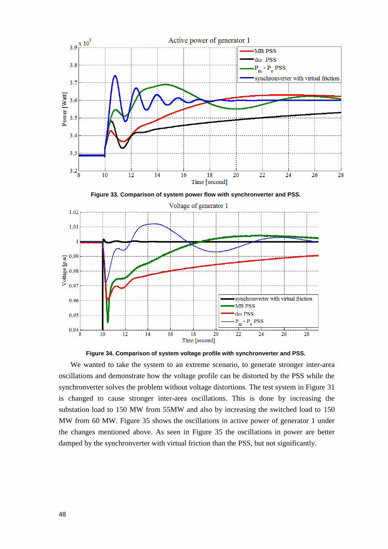
48
Figure 33. Comparison of system power flow with synchronverter and PSS.
Figure 34. Comparison of system voltage profile with synchronverter and PSS.
We wanted to take the system to an extreme scenario, to generate stronger inter-area
oscillations and demonstrate how the voltage profile can be distorted by the PSS while the
synchronverter solves the problem without voltage distortions. The test system in Figure 31
is changed to cause stronger inter-area oscillations. This is done by increasing the
substation load to 150 MW from 55MW and also by increasing the switched load to 150
MW from 60 MW. Figure 35 shows the oscillations in active power of generator 1 under
the changes mentioned above. As seen in Figure 35 the oscillations in power are better
damped by the synchronverter with virtual friction than the PSS, but not significantly.

49
Figure 35. Comparison of system power flow with synchronverter and PSS, with the switched load
increased to 150 MW (from 60 MW) and the substation load increased to 150 MW (from 55 MW).
Figure 36. Comparison of system voltage profile with synchronverter or PSS, under the same
conditions as in Figure 35.
As seen in Figure 36 the voltage profile on the generator terminals is distorted
significantly when the PSS solution is applied during strong inter-area oscillations. Figure
36 shows that even for strong inter-area oscillations the voltage profile of the generator
terminals remains unchanged when the oscillations are damped using synchronverters and
virtual friction. One must remember that in this example the PSS works on generators
which supply 90% of the power while the virtual friction works on inverters supplying only
10% of the power. In cases where the synchronverters supply much more power the results
will be much better in favor of the synchronverter. Since we have compared
synchronverters with virtual friction to synchronous generators with a PSS controller, it is
hard to say which solution would work better if both of them are implemented on the same
power source, either a synchronverter or a synchronous generator. We would like to test

50
both solutions on the same power source. We cannot create virtual friction between two
synchronous generators, however we can add an additional PSS controller to our
synchronverter algorithm. We assume that the synchronverter behaves similar enough to a
synchronous generator, so that we could actually apply to it a PSS control. The PSS
controller works on the induced voltage in the rotor. In our synchronverter algorithm we
assume that the derivative of the rotor current is 0 which is equivalent to assuming that the
voltage across the rotor is constant. But in reality small fluctuations in the rotor current
influence the flux in the rotor and thereby change the rotor voltage. This is good for us
since it means we can use the current to change the voltage on our imaginary rotor to
stabilize frequency fluctuations caused by inter-area oscillations using PSS control. In
Figure 37 we can see where we place our PSS controller in our algorithm. The proportional
gain qD stabilizes the voltage amplitude in the synchronverter terminals. By adding
another reference voltage from PSS control which depends on frequency fluctuations we
couple the voltage amplitude E with the frequency disturbance, Δf .
The washout filter constant wT in Figure 37 is chosen in the range of 1 to 10 seconds. The
synchronverter algorithm is run on a processor so it is discrete and not continuous. The
constant pK should be chosen such that it amplifies the disturbance in frequency
Figure 37. Synchronverter with PSS controller

51
sufficiently, but not higher than what the synchronverter can handle. We have found
10pK to be suitable. It is important to saturate the additional voltage from the PSS
control to be not more than 5% of the nominal voltage and not less than -10% of the
nominal voltage. The implementation in Figure 37 is a basic standard control structure of a
PSS. There are better implementations of PSS controllers but this is good enough for our
test. In order to check that this PSS controller actually does what it is supposed to do we
designed a test system of two synchronverters with a switched load between them
connected via a high impedance line. This should generate inter-area oscillations when the
loads are switched. I will not give an exact description of this simple system since the exact
parameters are not important, only the fact that inter-area oscillations are generated
between 2 synchronverters. The figure below presents the phase difference between the
synchronverters virtual rotor angle, .
Figure 38. Proof of concept for PSS implementation in a weakly connected two synchronverter
system.
We see in Figure 38 that until t=8s there are no oscillations. At t=8s the load changes and
the load sharing between both synchronverters changes as well. We see that the blue line
representing the case where the synchronverters have neither PSS nor virtual friction, has
oscillations that do not decay until the load changes back to its previous value at t=16s. The
red line represents the case where both the synchronverters have a PSS controller. We see
that the oscillations decay but the sharing of the load, located between the two
synchronverters in the middle of the line connecting them, is different. It is hard to say
whether this is good or bad since it depends on the application. In such a simple system
there is no ideal load sharing. The teal line represents the case where the synchronverters
have virtual friction between them and we obtain better decay of the oscillation. The black
line represents the scenario where the synchronverters have virtual friction between them
and also a PSS controller. There is a slight improvement in the decay of oscillations but it is
hard to tell whether this is a real improvement (compared to only having virtual friction) or
some side effect due to simulation approximations. To summarize we see that the proposed

52
PSS controller does indeed work as it should in a synchronverter. We would like to test if
the synchronverter with PSS controller performs as well as the synchronverter with virtual
friction in the system described in Figure 31. Then we can truly understand which solution
is better for the synchronverter operating in a system with synchronous generators. Here we
wanted to see the performance of each solution clearly so we run the simulations under the
extreme conditions described in Figure 35.
Figure 39. Comparison of the synchronverters from the test system in Figure 31 in 4 different
operation modes, with and without PSS and virtual friction.
We see in Figure 39 that the difference between the blue line which describes the results
under no PSS or virtual friction between synchronverter, and the green line with PSS only
is very small. Since the PSS is placed in the synchronverters which only supply 10% of the
power and are not the cause of the oscillations it does not do much. This is unlike the
simulation in Figure 38 where only synchronverters (and no synchronous generators) are
involved with PSS added to them. The red line in Figure 39 shows that using virtual
friction dampens inter-area oscillations like in Figure 35. The black line which combines
both PSS and virtual friction shows very little improvement. The results in Figure 39 are
different from the results for the two synchronverter system in Figure 38, since here the
synchronverters are not the cause of oscillations, the synchronous generators are. We see
that not only virtual friction is a better solution than PSS (when they both operate on the
synchronverters) but also that it can help in cases where the PSS does not help.
It is important to note that communication systems have delays. These delays may
interfere with our virtual friction implementation. It has been checked that for small delays
of up to 2 milliseconds the results do not differ by much. I have chosen not to attach these
results since this issue requires more research then I have conducted so far.

53
7.3. The Pogaku-Prodanovic-Green (PPG) inverter and
inter-area oscillations
We would like to investigate the performance of the system described in Figure 31 if
instead of synchronverters we use a conventional inverter. For this purpose we have
selected a very advanced inverter controller developed by N. Pogaku, M. Prodanovic and
T.C. Green in [23]. This controller has frequency-power droop control as well as advanced
load sharing capabilities. Below are the control block diagrams of this inverter as they
appear in [23]:
Figure 40. General inverter block diagram. P is the Park transform and an inverse Park transform
is done after the calculations in the current controller, before the PWM generator and switches.
Figure 41. Power controller of th PPG inverter. 𝝎𝒄 is an LPF cut-off frequency for high harmonic
filltering of active and reactive power. 𝝎𝒏 is a referance frequency frame within the range of
allowed operational frequencies, that will set the power 𝑷𝒏 transferred to the grid at nominal grid
frequency corresponding to the equation 𝝎𝒏 − 𝒎𝒑𝑷𝒏 = 𝝎𝒈𝒓𝒊𝒅 , where 𝝎𝒈𝒓𝒊𝒅 is the grid nominal
frequency and 𝑷𝒏 is the active power after the LPF. The actual power that will flow to the grid is
bigger. In order to calculate the actual power supplied to the grid we must also add the power that
is cut by the filter. This is not easy to compute, since we do not know the effect of the switches
and other non linear elements in the grid. We simply tuned the value of 𝝎𝒏 until we got the wanted
nominal power for the simulations. 𝒎𝒑 is a droop gain calculated by 𝒎𝒑 = (𝝎𝒎𝒂𝒙 − 𝝎𝒎𝒊𝒏) 𝑷𝒎𝒂𝒙⁄
where if we consider negative frequency drooping (extra power for frequency below nominal) we
need to put 𝟐𝑷𝒎𝒂𝒙. 𝑽𝒏 is the nominal voltage amplitude (phase to ground) of the inverter and 𝒏𝒒 is
calculated by (𝑽𝒎𝒂𝒙 − 𝑽𝒎𝒊𝒏)/𝑸𝒎𝒂𝒙 . This value represents the voltage drooping, the higher the
value of 𝒏𝒒, the less compansation in VAr is given for maintaning constant voltage. This
parameter requires tuning. 𝜽𝑷𝑷𝑮 is the estimeted grid angle, used in the Park and inverse Park
transformations.
𝜔 PPG

54
Figure 42. Voltage controller of the PPG inverter. 𝑲𝒑𝒗 and 𝑲𝒊𝒗 are PI controller constants for the
voltage controller and 𝑪 is The value of the filter capacitor, 𝑪𝒇 used to compute the effect of
filttering on the output voltage and 𝑭 is the current feed-forward gain. 𝑭 is used to improve the
disturbance rejection of the inverter system.
Figure 43. Current controller of the PPG inverter. 𝑲𝒑𝒄 and 𝑲𝒊𝒄 are PI controller constants for the
current controller and 𝑳 is the value of the output inductor, 𝑳𝒄. The value of this inductor is used
since we want to control the output filter inductor current and not the current before the filter.
Values For 40 MW PPG inverter
Parameter Value
𝑳𝒇 0.0725 nH
𝑪𝒇 5.52 mF
𝑳𝒄 0.04575 nH
𝑲𝒑𝒗 500
𝑲𝒊𝒗 1000
𝑲𝒑𝒄 10.5
𝑲𝒊𝒄 5000
𝑭 0.75
𝝎𝒏 323.4593 rad/second
𝑽𝒏 563 V

55
𝝎𝒄 31.4 rad/second
𝒎𝒑 0.35 (𝑟𝑎𝑑
𝑠𝑒𝑐𝑜𝑛𝑑) /𝑀𝑊
𝒏𝒒 60 𝑉/𝐺VAr
Table 2. Values of parameters for a 40 MW PPG inverter working in a 50 Hz grid.
One can easily see that this inverter uses an LCL filter like the synchronverter and it also
has frequency-power drooping and voltage-reactive power drooping like in the
synchronverter. This makes it easy for us to build an inverter model with parameters equal
to those of the synchronverter.
An additional synchronization block should also be added to this inverter. We have
designed a synchronization process which is almost identical to the one in our self-
synchronized synchronverter. We found that the resulting system behaves similarly to the
one containing synchronverters without virtual friction. This means that synchronverters
have the advantages of other advanced inverters, and this is probably due to their fast
frequency-power droop, which does not suffer from mechanical limitations and delays like
the frequency-droop loop of a real generator. The following figure is the comparison of the
synchronverter and this inverter, which we will refer to as PPG inverter, when we put them
in the system shown in Figure 31.
Figure 44. For the system in Figure 31, comparison of behaviour with inverter and
synchronverter (without virtual friction).
8. Eilat –Ktura grid section: a case study
So far we have tested the synchronverter in simulated systems, some of which we
designed ourselves for some specific tests and others were based on systems in SimPower
examples. To verify that the synchronverter actually helps in a real system we should test it
on a real system. For this purpose we have chosen the grid section between Eilat and Ktura.
Eilat is the southernmost city in Israel. This means that electricity produced mostly in
Hadera power station has to travel long distances to reach Eilat. This is very costly which
makes Eilat a perfect candidate for renewable sources, along with the fact Eilat is sunny

56
most of the year. We obtained data from the IEC concerning line parameters, synchronous
generators found in Eilat, renewable sources currently located in Ktura and other sources
that will be available in the future. The north line from the center of Israel to Ktura was
given similar values as the line from Ktura to Eilat, only that the former is six times longer.
The grid from the north is modeled as an infinite bus. In Figure 45 we see the full scheme
of the system.
Figure 45. Schematics of Eilat-Ktura grid section.
The simulation scenario is as follows: first we connect the generators in Eilat to the
infinite bus, wait for 8 seconds until the system stabilizes. After the system stabilizes, at
t=8s, the inverter in Ktura is connected. It takes another 8 seconds for the system to
stabilize. Assume that when the inverter in Ktura is connected along with the generators in
Eilat, we get a scenario where the local load is balanced by the local power production.
This is a reasonable scenario since it is expensive to bring power from the north to Eilat.
Two seconds later at t=18s the line from the north to Ktura is disconnected thereby creating
an electrical island. This could happen for maintenance reasons or faults somewhere along
the line from Ktura to the north. It is important to note that currently the IEC does not allow
islanding but this situation would probably change in the future. The newly created
electrical island in Eilat-Ktura grid section starts oscillating in frequency and power. It
takes almost 15 seconds until the oscillations decay. After another 17 seconds at t=35s a
three phase fault occurs in Eilat. This is an extreme but possible scenario. Short circuits
occur frequently in a power grid. Most of them are one phase faults that last for a short
duration and consume little power. We consider this three phase short circuit in three
scenarios: with the resistance between the phases (in Eilat) being 10Ω, 1Ω and 0.1Ω. In
the first scenario the three phase fault causes a 2% frequency decrease at the Ktura and
Eilat generators, due to the extra power dissipated in the high voltage line and also in the
resistors of the short circuit. The frequency in Eilat also decreases in the case of 1Ω short
circuit, but it increases for 0.1Ω, as is normal for generator near a total short circuit (where
terminal voltage drops near zero). In each of the three cases, a phase difference develops
between Eilat and Ktura during the short circuit and the islanded system oscillates after the
short circuit is removed. The recovery of the system from the fault depends on the type of
inverter used in Ktura. We want to compare the synchronverter with our PPG inverter

57
described in the previous chapter. Today there are no inverters that allow positive
frequency-power drooping, meaning that if the frequency drops the inverter cannot supply
additional power since it has no energy storage. This is why we need to update the PPG
inverter to only support negative power-frequency drooping. This is done by saturating the
power output if the signal P from the frequency droop is larger than 𝑃𝑛as shown in Figure
45 below. Notice that 𝑃𝑛 is the nominal power after the LPF, this is lower than the actual
power flowing to the grid at nominal grid frequency, see Figure 41 for more details.
Figure 46. Updated power controller of the inverter designed in [23] (compare with Figure 41).
In Figure 46 we see that if the power the inverter has to generate (due to frequency drop)
is larger than the nominal power then, the frequency-power droop characteristic changes so
that the frequency is still tracked by the inverter but the power does not exceed nominal
power.
We have run three simulations: one with the synchronverter as the inverter at Ktura, the
second with the PPG inverter as the inverter at Ktura and a third with a synchronous
generator instead of the inverter at Ktura. We have run these simulations to compare the
performance of the synchronverter and the PPG inverter. The synchronization process (see
below in Figure ) is equally good for the synchronverter and the updated PPG inverter and
they both synchronize better than a synchronous generator.
Figure 47. Synchronization of the inverter at Ktura to the grid (frequency in Ktura).
Assuming that 89 MW are generated by synchronous generators in Eilat, and 40 MW
are generated by an extra unit 52 km to the north in Ktura, generation and consumption are
balanced. We have simulated 3 options for this extra unit: synchronverter, updated PPG
inverter and synchronous generator. The Eilat-Ktura grid section is islanded at t = 18s and
at t = 35s a 150 ms short circuit occurs. In each of the following scenarios when the extra
unit in Ktura is a synchronous generator the local grid of Eilat-Ktura loses stability, leading
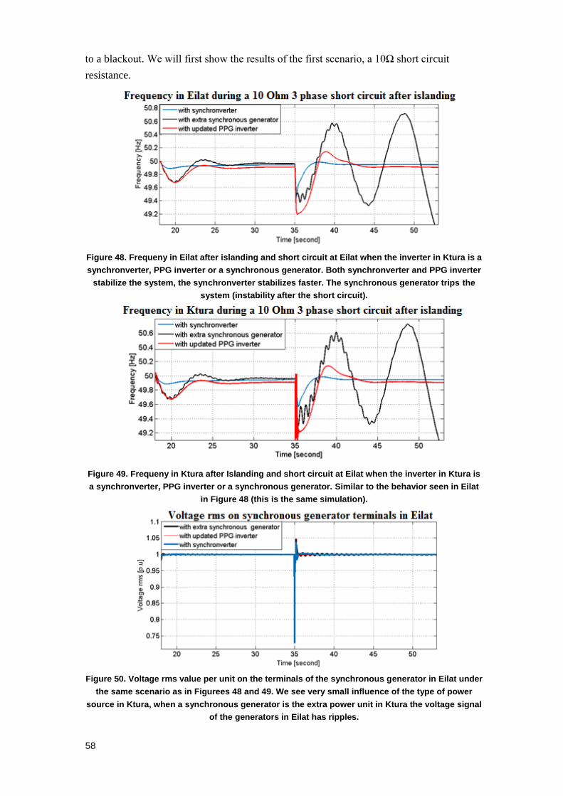
58
to a blackout. We will first show the results of the first scenario, a 10Ω short circuit
resistance.
Figure 48. Frequeny in Eilat after islanding and short circuit at Eilat when the inverter in Ktura is a
synchronverter, PPG inverter or a synchronous generator. Both synchronverter and PPG inverter
stabilize the system, the synchronverter stabilizes faster. The synchronous generator trips the
system (instability after the short circuit).
Figure 49. Frequeny in Ktura after Islanding and short circuit at Eilat when the inverter in Ktura is
a synchronverter, PPG inverter or a synchronous generator. Similar to the behavior seen in Eilat
in Figure 48 (this is the same simulation).
Figure 50. Voltage rms value per unit on the terminals of the synchronous generator in Eilat under
the same scenario as in Figurees 48 and 49. We see very small influence of the type of power
source in Ktura, when a synchronous generator is the extra power unit in Ktura the voltage signal
of the generators in Eilat has ripples.

59
Figure 51. Voltage rms value per unit on the terminals of the extra power unit at Ktura. We see that
the synchronverter maintains higher voltage levels than both PPG inverter and synchronous
generator and that the PPG inverter has the most stable voltage level on its terminals.
Figure 52. The active power supplied from Ktura by the synchronverter, PPG inverter or
synchronous generator under the scenario from Figures 48, 49. The synchronverter delivers more
power although both inverters and the synchronous generator are designed to supply 40 MW
nominal power, and maintains better stability. The synchronous generator causes many ripples.
Figure 53. The reactive power supplied from Ktura by the synchronverter, PPG inverter or
synchronous generator under the scenario from Figures 48, 49. The synchronverter supplies
more reactive power, which explains the high level of voltage on its terminals shown in Figure 51.
The synchronous generator causes ripples.

60
When we take the system to a more extreme situation, a 1Ω resistance in the short circuit,
we get similar results that highlight the advantage of the synchronverter versus the PPG
inerter.
Figure 54. Frequeny in Eilat after Islanding and 1Ω short circuit at Eilat at t = 35s when the
inverter in Ktura is a synchronverter, PPG inverter or a synchronous generator. Both
synchronverter and PPG inverter stabilize the system, the synchronverter stabilizes faster. The
synchronous generator trips the system (instability after the short circuit).
Figure 55. Frequeny in Ktura after Islanding and short circuit at Eilat when the inverter in Ktura is
a synchronverter, PPG inverter or a synchronous generator. Similar to the behavior seen in Eilat
in Figure 54 (this is the same simulation as Figure 54).

61
Figure 56. Voltage rms value per unit on the terminals of the synchronous generator in Eilat under
the scenario from Figure 54. We see very small influence of the type of power source in Ktura,
when a synchronous generator is the extra power unit in Ktura then the voltage signal of the
generators in Eilat causes ripples.
Figure 57. Voltage rms value per unit on the terminals of the extra power unit at Ktura under the
scenario from Figure 54. We see that the Synchronverter maintains higher voltage levels than
both the PPG inverter and the synchronous generator and that the PPG inverter has the most
stable voltage level on its terminals.
Figure 58. The active power supplied from Ktura by the synchronverter, the PPG inverter or the
synchronous generator under the scenario from Figure 54. The synchronverter delivers more
power although both inverters and the synchronous generator are designed to supply 40 MW
nominal power, and maintains better stability. The synchronous generator causes many ripples.

62
Figure 59. The reactive power supplied from Ktura by the synchronverter, the PPG inverter or the
synchronous generator under the scenario from Figure 54. The synchronverter supplies more
reactive power, which explains the high level of voltage on its terminals shown in Figure 56. The
synchronous generator causes ripples.
We wanted to see the behavior of the systems in a classical short circuit, when the
voltage on the synchronous generators terminals drops almost to zero during the 150ms of
the short circuit. For that we reduced the resistance of the short circuit to 0.1Ω. This case is
different from the previous two since during a full short circuit the synchronous generators
cannot supply any power to the system because the voltage is zero. This causes the
generators to work in under loaded conditions, such conditions cause the frequency to jump
up and mechanical damage could be inflicted to the rotating parts of the generator. This
only happens if the frequency jumps too high or for a long time period, the limitations
depend on the age of the generator and the manufacturers design.
Figure 60. Frequency in Eilat with a full short circuit (0.1Ω) in Eilat occurring at t = 35s. We see
that the frequency rises during the fault as expected. The recovery of the system with the
synchronverter in Ktura is better than with the PPG inverter. When Ktura has a synchronous
generator then the system trips like in the previous short circuit scenarios.

63
Figure 61. Frequency in Ktura with a full short circuit in Eilat occurring at t = 35s. We see that the
frequency in Ktura behaves the same as in Eilat. Frequency rises during the fault, the
synchronverter gives fastest recovery and with the synchronous generator there is a blackout.
Figure 62. Voltage rms value per unit on the terminals of the synchronous generators in Eilat with
the scenario as in Figure 60. We see very small influence of the type of power source in Ktura.
The synchronverter gives better results, lowest voltage jump during recovery.
Figure 63. Voltage rms value per unit on the terminals of the extra power unit at Ktura with the
scenario as in Figure 60. We see that the synchronverter maintains higher voltage levels than
both the PPG inverter and the synchronous generator and that the PPG inverter has the most
stable voltage level on its terminals.

64
Figure 64. The active power supplied from Ktura by the synchronverter, PPG inverter or
synchronous generator with the scenario as in Figure 60. The synchronverter delivers more
power although both the PPG inverter and the synchronous generator are designed to supply 40
MW nominal power, and maintains better stability. The synchronous generator causes many
ripples.
Figure 65. The reactive power supplied from Ktura by the synchronverter, PPG inverter or
synchronous generator with the scenario as in Figure 60. The synchronverter supplies more
reactive power, which explains the high level of voltage on its terminals shown in Figure 63. The
synchronous generator causes ripples.
Figures 48 to 65 shows that the synchronverter not only gives faster recovery time from
faults but also reduces the effect of the faults themselves. We also see that after islanding,
the power flow from Ktura decreases in the case of the PPG inverter, and increases in the
cases of the synchronous generator and the synchronverter, see Figures 52, 58 and 64. This
is due to negative drooping that allows the synchronverter and synchronous generator to
supply more than the nominal active power to stabilize the frequency. While the PPG
inverter does handle the faults well, we see that the synchronous generator trips. This is
probably due to the slow response time of the synchronous generator frequency drooping.
Inverters have no mechanical parts, which makes their response faster than that of
conventional generators. This quality is very important but it may also cause problems if
the inverters have no additional energy storage. In some cases the grid may have a fault and

65
we may want the grid to maintain the existing performance. This will not be possible
without additional energy to compensate the losses caused by the fault. For this reason the
synchronverter along with a small energy storage unit offers the best support for grid
stabilization.
We also wanted to check what would happen if the extra power that is supposed to come
from the synchronverter has a time delay of 200 milliseconds. This delay can be a result of
the dynamics of MPPT or energy storage device discharge. There is no need to recreate all
3 scenarios introduced previously since the effect on the synchronverter should be the same
regardless of the fault itself. We choose to show this in the first scenario where the
resistance of the fault is 10Ω. In Figure 66 below we see that the differences, in frequency
which also corresponds to active power flow, with and without delay are negligible. There
is no effect on the voltage or reactive power from this delay in extra power supply, so we
have chosen not to attach the corresponding plots.
9. A synchronverter based energy storage device for
grid stabilization
This chapter is based on my intuition and more work is needed to truly understand the
advantages a synchronverter can provide while operating in an energy storage device.
Usually energy storage is used in emergencies when a fault of some sort occurs and
disconnects the user from the grid. In such a scenario the operating algorithm of the energy
storage inverter can be basic and simple. Indeed there are no stability problems for low
power energy supply in off grid operation. Another use for energy storage which is less
common is providing additional energy when the demand exceeds the available power
supply. This can happen on cold nights when people turn on heating boilers or on hot
summer days when people turn on air-conditioning systems. There could also be other
Figure 66. Ktura-Eilat simulation of a 10Ω short circuit in Eilat with a synchronverter
in Ktura. The scenario is repeted twice with and without time delay of the
synchronverter for extra power.This Figure shows the frequency in Eilat. The two
curves overlap.

66
circumstances but these are the main scenarios. Usually when an energy storage device is
used together with the grid it must work under some basic regulations. Since the power
energy storage can supply is negligible relative to the grids power most inverters today will
only work under these regulations.
We suggest a new use for energy storage devices. As shown in the last chapter inverters
have certain advantages such as zero delay frequency-power drooping which can
considerably contribute to grid stability. If we use emergency storage for grid stabilization
it will help justify the cost of existence of such devices and may even help make the grid
more robust (which is especially important in places with poor infrastructure). We suggest
keeping the energy storage devices always connected with nominal power 0W. The inverter
is operated with the synchronverter algorithm.
To demonstrate how this could work we need to build a model of a power grid which
includes low voltage, medium voltage and high voltage grid sections, each of which plays a
different role in delivering power for consumers. After some research we designed the
following grid:
Figure 67. Scheme of power grid with low, medium and high voltage parts. The line is modeled
using the distributed model of power lines.
In this scheme the high voltage part comes from a faraway large power station and in the
medium voltage part there is a local factory with industrial power station that can provide
all electrical needs for the factory and a nearby city. The low voltage part is simulating a
small city with a 10MW power consumption divided in to two branches where one branch
consumes 2MW more than the other. There are power factor compensators in each branch.
On the branch with the bigger load there is a laundromat or a facility which uses a large
1MW motor, which is modeled using a synchronous machine with a constant negative
mechanical torque input (which means a constant mechanical load). We also add load
switching noises of about 1-1.5% of the branch loads to simulate a more realistic power
grid. It is important to note that in an actual grid there are more branches in the low voltage
area and FACT devices, see Chapter 11 pp. 627-684 in [16], which helps regulating the
voltage and the power factor. To make the simulation faster we ignore this. We do not
claim that this omission will not matter but this is not important in the simple proof of
concept of an always connected emergency energy storage device whose inverter works as

67
a synchronverter. After some simulations where we connected the synchronverter to
various parts of the grid we found that the weakest spots of the grid are the elements which
have complex dynamics such as the motor or synchronous generator. So the best place to
put a stabilizing device is near these elements.
To check if there are improvements when a synchronverter is added, we caused a fault
near one of the medium to low voltage transformers on the medium voltage side. The fault
is a 3 phase fault of 10Ω for duration of 150 milliseconds. Unfortunately placing a
synchronverter with 0W nominal power with the regular algorithm did not contribute much
to grid stability. This is probably since the infinite bus is strong enough to keep the system
stable so the synchronverter was not really needed.
This got us looking for an idea for making the synchronverter more meaningful even in
the presence of an infinite bus. On the basis of the effect of virtual friction on inter-area
oscillations we expected that there must be a way to cause similar decay in local
oscillations, or at least in inter-area oscillations, using only one synchronverter. Indeed this
can be achieved by using an one way virtual friction between the synchronverter and some
oscillating element, either a synchronous generator or a motor. More precisely, we add
another torque to the right side of (4.4). For a generator this torque should be
( )vf e mT p p where mp is the mechanical power the generator receives from the
governor and ep is the generator’s output electrical power. Typically in a synchronous
generator, the mechanical power is slowly varying and the electrical power changes fast
which leads to oscillations in the system. The synchronverters fast frequency drooping can
help the system stabilize faster by compensating for the slow change in mechanical torque.
For a motor the torque has an identical expression given by ( )vf e mT p p where mp
is the mechanical load’s power and ep is the electrical power being absorbed by the motor.
This means that the mechanical power acts like a constant nominal reference power for the
generator or the motor and the electrical power is the dynamical fast changing power that is
absorbed or consumed by the motor/generator. One important fact that needs to be
mentioned is that the power that the generator (motor) produces (consumes) is different,
usually bigger than the power the synchronverter produces. Hence we need to normalize
the additional torque. The chosen normalization is as follows 2syn Genchvf vf max maxT T P P .
Therefore if the amplitude of oscillation of power in the generator or motor is maxgenP or
maxmotP , then the synchronverter can supply for a short period up to twice its maximum
power which is usually the nominal power it was designed to output. We recommend that
in the future, after checking the feasibility of inverters to supply higher power for short
durations, the normalization should change and maybe we can use synchronverters
designed for nominal power P to output momentarily power 5 P or more. Simulations
indicate that this helps considerably in the decaying of oscillations and does not require
bigger energy storage (since the oscillations last a very short period of time).

68
We have run 6 different scenarios to check this idea. The first scenario is simply the
system from Figure with the fault mentioned in the previous page. This scenario is the
reference scenario which we want to improve using the synchronverter. The second
scenario is adding a 2MW nominal power synchronverter in parallel to the motor and load
on the low voltage side. Here we add a one sided virtual friction torque between the
synchronverter and the motor. The third scenario is adding a synchronverter of 5MW
nominal power in parallel to the synchronous generator on the medium voltage side with a
one sided virtual friction torque between them. The fourth scenario includes both
synchronverters from scenario 2 and 3 to show that they work better together without
disturbing each other. In the fifth scenario We used the system from scenario four and
added another synchronverter of 10 MW nominal power on the high voltage side in parallel
to the infinite bus. We also added an additional virtual friction between this synchronverter
and the synchronverter on the medium voltage side. This was to verify if the main problem
is the oscillations between the infinite bus and the synchronous generator and if so the
virtual friction between the two synchronverters parallel to them should help considerably.
The last scenario was the same system from scenario five without any virtual friction
torques. The point of this scenario is to show that without these torques the synchronverters
with 0W nominal power do not affect the system as much as they would with them. First in
Figure 68 we plot the power of the synchronverter near the synchronous generator and the
power of the generator from scenario three in addition to the power of the same
synchronverter in scenario six without the one sided virtual friction. Similarly in Figure 69
we plot the power of the synchronverter in the low voltage side and the power of the motor
from scenario four together with the power of the synchronverter from scenario six without
the one sided virtual friction.
Figure 68. Output power of synchronous generator and synchronverter attached to it with and
without one sided virtual friction. synchronverter connects at t=3.2s and the fault starts at t=5s
and lasts until t=5.15s.
We can clearly see in Figure 68 that the power from the synchronverter has a very small
phase difference with the power from the generator whether or not there is a one sided

69
virtual friction between them. When this friction is absent we see that the synchronverter
reacts weakly.
Figure 69. Input power of 1MW synchronous motor and 5 MW load, and synchronverter attached
to it with and without one sided virtual friction. Synchronverter connects at t=3.2s and the fault
starts at t=5s and lasts until t=5.15s.
We see in Figure 69 that the motor is behaving like the generator in Figure 68 only much
smaller fluctuations in power. Without the one sided virtual friction the synchronverter
hardly reacts to motor power changes. Before presenting the frequency and voltage of both
the generator and motor in the 6 different scenarios in the next several pages, we
summarize the scenarios in the table below:
Scenario 1 No synchronverters present
Scenario 2 2 MW synchronverter on low voltage side
with one sided virtual friction with motor
Scenario 3 5MW synchronverter on medium voltage
side with one sided virtual friction with
generator
Scenario 4 Synchronverter on medium and low voltage
sides with corresponding virtual friction
with the generator and the motor.
Scenario 5 Synchronverter on low voltage side with
one sided virtual friction with the motor
and one sided virtual friction between
medium voltage side synchronverter and
synchronous generator and virtual friction
between medium voltage side
synchronverter and high voltage side
synchronverter
Scenario 6 3 synchronverters are present without
virtual friction of any kind
Table 3. Summary of the 6 tested scenarios for synchronverter use in energy storage.

70
For readability I have divided the plots to 3 scenarios each. Figure 70 present the three
worst attempts to stabilize the synchronous generator frequency and Figure 71 presents the
three best solutions for stabilizing the synchronous generator frequency.
Figure 70. Synchronverters connect at t=3.2s, fault occurs between t=5s to t=5.15s. We see that
with three synchronverters but without any virtual friction there is a small improvement and with a
synchronverter in the low voltage side with one sided virtual friction to the motor we see some
improvement after 7 seconds.
Figure 71. Synchronverters connect at t=3.2s and fault occurs between t=5s to t=5.15s. We see
that scenario 4 which includes 2 synchronverters with one sided virtual friction to the motor and
generator gives the best results. Adding another synchronverter in the high voltage side with
virtual friction to the synchronverter in the medium voltage side does not improve the results.
This is probably due to the fact that these oscillations are not inter-area but are more local in
nature.

71
Figure 72 present the three worst attempts to stabilize the synchronous motor frequency
and Figure 73 presents the three best solutions for stabilizing the synchronous motor
frequency.
Figure 72. Synchronverters connect at t=3.2s and fault ocurrs between t=5s to t=5.15s. We see
that the synchronverter on the medium voltage side does not help the motor performance
irrespective of whether there is one sided virtual friction between that synchronverter and the
synchronous generator.
Figure 73. Synchronverters connect at t=3.2s and fault ocurrs between t=5s to t=5.15s. We see
that scenario 4 which includes 2 synchronverters with one sided virtual friction to the motor and
generator gives the best results. Adding a synchronverter with one sided virtual friction to the
motor in the low voltage side does help, however since the oscillations in the synchronous
generator are much stronger and are not damped by the synchronverter on the low voltage side,
the effect of the synchronverter is limited. When we add both generator and motor with
synchronverters we see the strong effect of one sided virtual friction in the low voltage side
between the synchronverter and the motor.
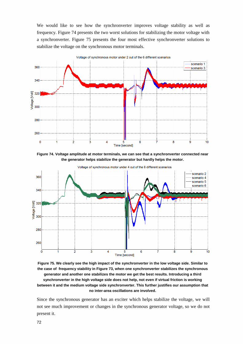
72
We would like to see how the synchronverter improves voltage stability as well as
frequency. Figure 74 presents the two worst solutions for stabilizing the motor voltage with
a synchronverter. Figure 75 presents the four most effective synchronverter solutions to
stabilize the voltage on the synchronous motor terminals.
Figure 74. Voltage amplitude at motor terminals, we can see that a synchronverter connected near
the generator helps stabilize the generator but hardly helps the motor.
Figure 75. We clearly see the high impact of the synchronverter in the low voltage side. Similar to
the case of frequency stability in Figure 73, when one synchronverter stabilizes the synchronous
generator and another one stabilizes the motor we get the best results. Introducing a third
synchronverter in the high voltage side does not help, not even if virtual friction is working
between it and the medium voltage side synchronverter. This further justifies our assumption that
no inter-area oscillations are involved.
Since the synchronous generator has an exciter which helps stabilize the voltage, we will
not see much improvement or changes in the synchronous generator voltage, so we do not
present it.
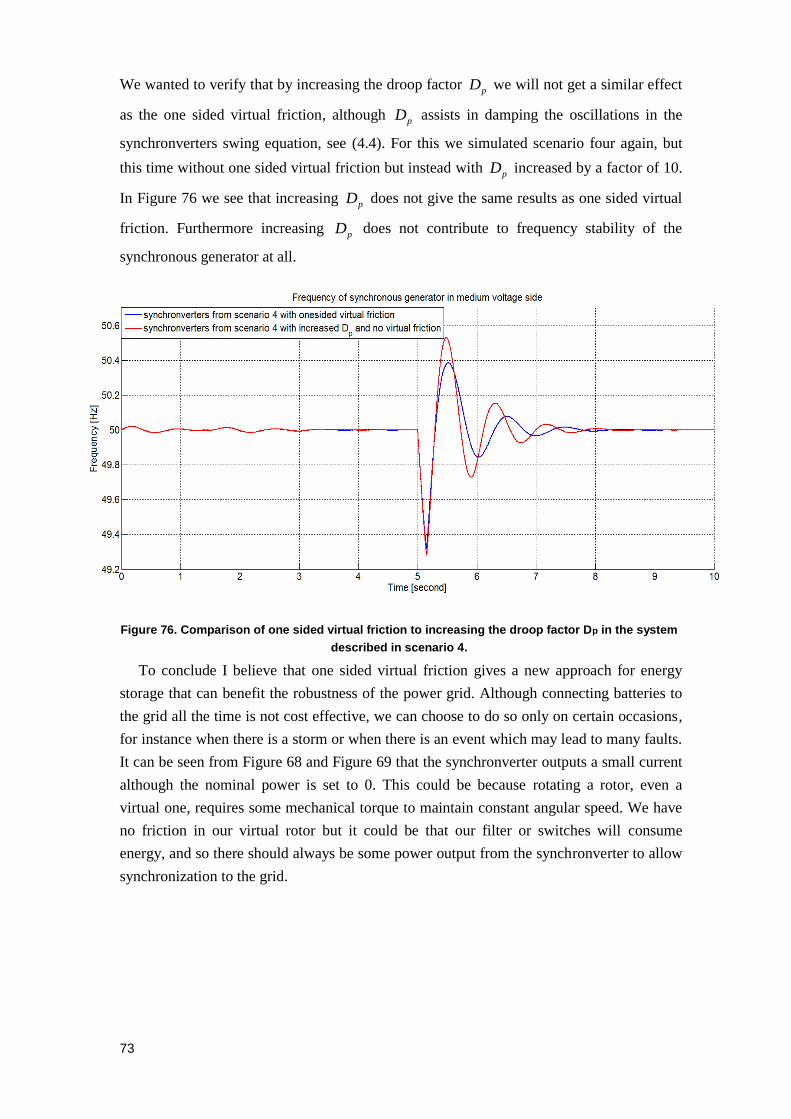
73
We wanted to verify that by increasing the droop factor pD we will not get a similar effect
as the one sided virtual friction, although pD assists in damping the oscillations in the
synchronverters swing equation, see (4.4). For this we simulated scenario four again, but
this time without one sided virtual friction but instead with pD increased by a factor of 10.
In Figure 76 we see that increasing pD does not give the same results as one sided virtual
friction. Furthermore increasing pD does not contribute to frequency stability of the
synchronous generator at all.
Figure 76. Comparison of one sided virtual friction to increasing the droop factor Dp in the system
described in scenario 4.
To conclude I believe that one sided virtual friction gives a new approach for energy
storage that can benefit the robustness of the power grid. Although connecting batteries to
the grid all the time is not cost effective, we can choose to do so only on certain occasions,
for instance when there is a storm or when there is an event which may lead to many faults.
It can be seen from Figure 68 and Figure 69 that the synchronverter outputs a small current
although the nominal power is set to 0. This could be because rotating a rotor, even a
virtual one, requires some mechanical torque to maintain constant angular speed. We have
no friction in our virtual rotor but it could be that our filter or switches will consume
energy, and so there should always be some power output from the synchronverter to allow
synchronization to the grid.

74
10. Future work and conclusions
We have seen that synchronous generators are not always stable, but when they are near
a stable equilibrium, which is usually the case in a well-designed electrical grid, they are
not only stable but can be analyzed using a simpler reduced model. We have also seen that
in this reduced model rotor current does not depend on stator current and other state
variables which means that the rotor current will stabilize to a constant value. In the future
we will try to accurately identify the region of attraction where the reduced third order
model remains stable. We also want to see if the synchronverter behaves like the fifth order
model of the synchronous generator, which we know is a fairly accurate model of a real
generator that has known and verified control schemes. This can help choose the
parameters for the synchronverter. In this work we have only examined a case where the
synchronous generator is connected to an infinite bus. We would like to study the case of
two connected generators for understanding the interconnection of generators and related
problems better.
We have seen from simulations that the synchronverter indeed works like a synchronous
generator in terms of frequency and voltage drooping. We have also seen that a grid formed
by two synchronverters behaves like a grid formed by a synchronous generator. We would
like to test this in a lab in the future, with actual equipment. Another issue for the future is
to diagnose and create a fault ride through behavior in the synchronverter which will
probably be similar to that in a synchronous generator.
We have introduced the idea of virtual friction between two generators or
synchronverters as another way to reduce inter-area oscillations. This idea has only been
demonstrated using simulations. It would be useful to develop a mathematical model of this
concept.
We have also examined the well-known solution to inter-area oscillations, PSS. The
efficiency of PSS in a synchronverter has not been properly studied. We have only shown
that it can be implemented, but we have not explored the best way to do it.
We have given some insights for the use of a synchronverter in energy storage devices.
Although there is no mathematical model, it is clear that once we have more energy
available during a fault, the less damage the fault will cause. We have also shown a way to
implement one sided virtual friction between a synchronverter and a synchronous machine
(generator or motor). Again there is a need to build a mathematical model of this.
Using data from IEC we have seen that the synchronverter is suitable for micro grids or
in cases when islanded operation is allowed in a large grid. In the future when the demand
for electricity would increase, the complexity of the grid will increase as well and simple
stability solutions will be hard to find. The synchronverter, with its flexibility, has a good
potential to provide elegant and simple solutions.

75
11. Bibliography
[1] J. Alipoor, Y. Miura and T. Ise, "Distributed generation grid integration using
virtual synchronous generator with adaptive virtual inertia", IEEE Energy Conversion
Congress and Exposition, Denver, Colorado, 2013, pp. 4546-4552.
[2] H.P. Beck and R. Hesse, "Virtual synchronous machine", 9th
International Conf. on
Electrical Power Quality and Utilization, Barcelona, Spain, 2007, pp.1-6.
[3] F. Blaabjerg, R. Teodorescu, M. Liserre and A.V. Timbus, "Overview of control
and grid synchronization for distributed power generation systems", IEEE Trans. on
Industrial Electronics, vol. 53 , 2006, pp. 1398-1409.
[4] F. Bullo and F. DӦrfler, "Synchronization and transient stability in power networks
and nonuniform Kuramoto oscillators", SIAM J. Control and Optim, vol. 50, 2012, pp.
1616-1642.
[5] E. Brown and G. Weiss, "Using synchronverters for power grid stabilization", IEEE
28th Convention of Electrical & Electronics Engineers in Israel (IEEEI), Eilat, 2014,
pp. 1-5.
[6] J. Driesen and K. Visscher, "Virtual synchronous generators", IEEE Power and
Energy Society General Meeting - Conversion and Delivery of Electrical Energy,
Pittsburg, PA, 2008, pp. 1-3.
[7] A.J. Ellison, "Electromechanical Energy Conversion", George G. Harrap and Co.
Ltd., London, 1965.
[8] R.W. Erickson and D. Maksimovic, "Fundamentals of Power Electronics", 2nd
edition. Kluwer Academic, Publishers, New York, 2004.
[9] S. Fiaz D. Zonetti, R. Ortega, J. Scherpen and A. van der Schaft, "A port-
Hamiltonian approach to power network modeling and analysis", European Journal of
Control, vol. 19, 2013, pp. 477-485. [10] A.E. Fitzgerald, C. Kingsley and S.D. Umans, "Electric Machine", McGraw-Hill,
New York, 2003.
[11] J.J. Grainger, W.D. Stevenson, "Power System Analysis", McGraw-Hill, New
York, 1994.
[12] J.M. Guerrero, J.C. Vasquez, J. Matas, M. Castilla, and L.G. de Vicuna, "Control
strategy for flexible microgrid based on parallel line-interactive UPS systems", IEEE
Trans. on Industrial Electronics, vol. 56, 2009, pp. 726-736.
[13] H.K. Khalil, "Nonlinear Systems", third edition, Prentice Hall, New Jersy 2002.
[14] V.K. Khanna, "Insulated Gate Bipolar Transistor (IGBT): Theory and Design",
Wiley-IEEE Press, Hoboken, NJ, 2003.
[15] M. Klein, G.J. Rogers and P. Kundur, "A fundamental study of inter-area
oscillations in power systems", IEEE Trans. on Power Systems, vol. 6, 1991, pp. 914-
921.
[16] P. Kundur, "Power System Stability and Control", McGraw-Hill, New York, 2009.
[17] G.A. Leonov, D.V. Ponomarenko and V.B. Smirnova, "Frequency-Domain
Methods for Nonlinear Analysis: Theory and Applications", World Scientific,
Singapore, 1996.
[18] Y. Mandel and G. Weiss, "Adaptive internal model based suppression of torque
ripple in brushless DC motor derives", Systems Science and Control Engineering, vol.
3, 2015, pp. 162-176.
[19] I.J. Nagrath and D.P. Kothari, "Electric Machines", third edition, Tata McGraw-
Hill, New Delhi, 2004.
[20] V. Natarajan and G. Weiss, "Almost global asymptotic stability of a constant field
current synchronous machine connected to an infinite bus", Proc. 53rd
IEEE Conf.
Decision and Control, Los Angeles, 2014, pp. 3272 -3279.

76
[21] B. Pal and B. Chaudhuri, "Robust Control in Power Systems", Springer Verlag,
New York, 2005.
[22] F.Z. Peng, L.M. Tolbert, and F. Khan, "Power electronics circuit topology – the
basic switching cells", IEEE Power Electronics Educational Workshop, Recife, Brazil,
2005, pp. 52 - 57.
[23] N. Pogaku, M. Prodanovic and T.C. Green, "Modeling, analysis and testing of
autonomous operation of an inverter-based microgrid", IEEE Trans. on Power
Electronics, vol. 22, 2007, pp. 613-623.
[24] P.W. Sauer and M.A. Pai : "Power System Dynamics and Stability". Stipes
Publishing, Champaign, IL, 1997.
[25] J. Strand, "Energy efficiency and renewable energy supply for the G-7 Countries,
with emphasis on Germany", International Monetary Fund, Working paper,
WP/01/299, 2007.
[26] A. Ulbig, T.S. Borsche and G. Andersson, "Impact of low rotational inertia on
power system stability and operation", IFAC World Congress, Cape Town, South
Africa, 2014.
[27] K. Visscher and S.W.H. de Haan, "Virtual synchronous machines for frequency
stabilization in future grids with a significant share of decentralized generation",
CIRED Seminar SmartGrids for Distribution, Frankfurt, Germany, 2008, paper no 118.
[28] J.H. Walker, "Large Synchronous Machines: Design, Manufacture and
Operation", Oxford University Press, Oxford, 1981.
[29] X. Yang and A. Feliachi, "Stabilization of inter-area oscillation modes through
excitation systems", IEEE Trans. Power Systems, vol. 9, 1994, pp. 494-502.
[30] A.A. Zea, "Power system stabilizers of the synchronous generetor, tuning and
performence evaluation", MSc thesis, Chalmers University of Technology, Goteborg,
Sweden, 2013.
[31] Q.-C. Zhong and T. Hornik, "Control of Power Inverters in Renewable Energy and
Smart Grid Integration", John Wiley & Sons, Ltd, West Sussex, United Kingdom,
2013.
[32] Q.-C. Zhong, P.-L. Nguyen, Z. Ma and W. Sheng, "Self-synchronized
synchronverters: Inverters without a dedicated synchronization units", IEEE Trans.
Power Electronics, vol. 29, 2014, pp. 617-630.
[33] Q.-C. Zhong and G. Weiss, "Synchronverters: Inverters that mimic synchronous
generators", IEEE Trans. Industrial Electronics, vol. 58, 2011, pp. 1259-1267.

77
12. Appendix - synchronverter parameters
Values used for the simulation of a 5 kW synchronverter
Variable Value
J synchronization 1e-5 2kgm
pD synchronization 1 Joulesecond
K synchronization 1000
R virtual 0.015
L virtual 4 mH
pK 4e-9
iK 2e-7
Synchronization limit 0.05 Volt
J 0.2 2kgm
pD 1.7 Joulesecond
K 5e4
qD 120 A
sR 0.152
sL 4.4 mH
C 10 μF
gL 2.2 mH
Switching period = sample time 1e-4 second
nv 330 Volt
f fM i initial condition 1.05 Volt second
h 20 rad second
e max ±400 Volt
P andQ LPF constant, see Figure 15 0.25second
P maximum 8 kW
P minimum 0 kW
Ilimiter – current limiter 25 Volt
Table 4. Parameters for 5 kW synchronverter.
Additional Comments:
The parameter synchronization limit is the voltage maximum difference we allow between
the EMF and the grid voltage when we connect the synchronverter. The voltage on the
capacitor is slightly higher than e , the synchronous internal voltage of the synchronverter.
The values for the synchronization process are application dependent. For faster

78
synchronization J and pD should be smaller, but there are cases where we may want
higher pD (for instance when the grid is noisy high synchronization pD is better). Ilimiter
is the maximum allowed voltage difference between the capacitor and the calculated EMF.
This is used to prevent large currents as described in Chapter 5. The values of K, R and L
should not be tuned since they are less application dependent and more nominal value
related. The PI controller values are not sensitive and should be tuned as required. The
values of K and qD are also application dependent, but the values given here are a good
starting point.
Values used for a PSS in a synchronverter
Variable Value
pK 10
T 1 second
LPF before PSS Simple averaging (old + new)/2
vfD (for virtual friction) Same as pD
pK PSS (optional) 25
iK PSS (optional) 0.15
High saturation value for PSS 0.05 nv
Low saturation value for PSS -0.1 nv
Table 5. Parameters for PSS and virtual friction in the synchronverter.
A more advanced method for a PSS is to add a PI controller after the LPF, the rest stays
unchanged. I have implemented this but noticed no improvement.

79
Values used for the simulation of a 1 MW synchronverter
Variable Value
J synchronization 1e-5 2kgm
pD synchronization 1.5 Joulesecond
K synchronization 1000
R virtual 200
L virtual 4 mH
pK 4e-6
iK 2e-5
Synchronization limit 0.02 Volt
J 40.5 2kgm
pD 337 Joulesecond
K 1e7
qD 5e4 A
sR 4e-4
sL 0.18 mH
C 140 μF
gL 0.029 mH
Switching period = sample time 1e-4 second
nv 563 Volt
f fM i initial condition 1.79 Volt second
h 20 rad second
e max ±680 Volt
P and Q LPF constant 0.0001second
P maximum 1.4 MW
P minimum 0 kW
Ilimiter – current limiter 150 Volt
Table 6. Parameters for a 1 MW synchronverter.
For any higher power synchronverter simply take the 1 MW values (except: internal
synchronous voltage maximum point e max, the amplitude reference nv , the frequency
reference h , the current limitation value limiter and the initial condition for rotor flux
f fM i since they are used for synchronization only, so there is no need to change them) and

80
multiply those with the nominal power of the synchronverter in MW. This works very well
and saves a lot of time recalculating.
LPF filtering of calculated values:
As mentioned in Chapter 5 some additional filtering is needed in the synchronverter
algorithm. I have chosen to implement these filters as a basic order one LPF with one
tunable parameter according to the following formula:
MeasuredValue OldValue
NewValue OldValueFilterParam
This means that if FilterParam is 1 we simply get no filtering meaning and
NewValue = MeasuredValue. For FilterParam = 2, we get a median between the old and
measured values. As FilterParam is increased the LPF is stronger, filtering more.
Although in some cases I chose high values for FilterParam, this is a not ideal since
filtering too strong will cause loss of information. It is recommended to tune the parameter
to as low a value as possible (of course the algorithm should work properly at this low
value).
Conversion of this discrete filter to continuous time:
Denote iy to be the new value, 1iy to be the previous value, iu to be the measured value,
and C to be the filter constant. Let the sample time be sT (this is the switching period of
the electronic switches). Then we rewrite the filter equation as
1
1i i
i i
u yy y
C
This can be rewritten as:
1( 1)i i iu Cy C y
We divide and multiply with sT to get:
1( 1) i ii i s
s
y yu y T C
T
This is the discrete version of the continuous-time differential equation:
1
( )( 1) 1s
y y uT C
From this we get the following transfer function for the filter from u to y :
1
( )( 1) 1s
H ssT C
.
We see that the DC gain is 1, so low frequencies are not being filtered and the time
constant of our filter is ( 1)sT C . From here we can calculate the 3dB frequency which is
3 1 ( 1)dB sf T C . In my simulations 0.1sT ms.

81
The calculated values that were filtered are:
Calculated Values with additional filtering
Variable FilterParam value and comments
gv (grid measured phase voltages) 1.66, 16.66 for extremely noisy grid
Q during synchronization 20 => 3 526HzdBf
gi (grid measured phase currents) 6
mv (calculated voltage amplitude) 10000
f fM i 1000 , only if a sharp drop in voltage occurs
40, if the synchronverter sets the grid then
this filter works only after initial stabilization
of frequency is achieved.
eT 12.5 - 50 only until initial stabilization
Q 100=> 3 101HzdBf
Table 7. Parameters for additional filters for the synchronverter.
The above filters were carefully built and tested in various simulations. They work for 5kW
as well as for 1MW synchronverters. Some tuning may be useful under certain conditions
but it is not recommended to deviate from these values. Overtuning or removing these
filters is dangerous for the synchronverters stability.

82
12.1. Basic system for detecting grid faults
In order to determine whether or not there is a grid fault we needed an additional function.
Commercial inverters have fault detection and handling system of their own, but for our
simulation process we had no predefined regulations for handling faults. We implemented a
basic function to detect the fault and disconnect only in the worst case scenarios of either
less than 30% grid amplitude for 150 ms or frequency decrease of less than 2%.
Detecting grid amplitude drop is easy, we only need to know the nominal voltage. Since
the voltage at the synchronverter terminals is always measured it is possible to calculate the
amplitude, store it as a variable and once it drops below 30% a timer starts counting to 150
ms. After that the system outputs a logical signal to the switches and disconnects the
synchronverter physically. Additionally the system will change the set mode of the
synchronverter to 'not set' and the synchronverter will start synchronizing again. The
synchronverter is set not to synchronize as long as the grid frequency is not in the proper
boundaries of 47.5 Hz and 51.5 Hz and the voltage amplitude is above 92% nominal value.
Frequency changes are more difficult to detect. We assume that the nominal grid frequency
is 50 Hz on each phase. For 50 Hz frequency the time period of the voltage is 20 ms. Let
the voltage on phase a be 0 Volt at t=0s, since the voltage on the other two phases have a
phase difference of 2 3 rad and 2 3 rad from phase a they will be 0 at time 3.3ms and
6.6ms respectively. We define 3 variables and store the voltages of phase ,a b and c at time
0s, 3.3ms and 6.6ms respectively. The variables are updated every 20 ms. Before updating
the 3 variables we check if the difference between the current and the previous values is
less than 5% of the nominal grid voltage amplitude. If they are not, then we know that the
grid frequency had changed. In this case the synchronverter checks if the new calculated
frequency (calculated by the synchronverter algorithm) is larger than the minimum
frequency allowed and if the rate of change is slower than 8 Hz per second, which is the
highest rate inverters are supposed to track. If one of these conditions is not met, then the
synchronverter is disconnected and it tries to synchronize again. This basic implementation
is sufficient for our needs since we only need to know drastic changes in frequency. For a
proper Ride Through Algorithm this simple grid fault check system needs a better
implementation.
The simulations were run with ode23tb solver, relative tolerance was set to 1e-3 or 1e-4
for noisy simulations. The recommended tolerance is 1e-3. According to Matlab this solver
is considered the best for simulations including SimPower elements. For some simulations
I had limited the max step size to 1e-4. Usually that works well but sometimes it slows the
simulation without improving results so it is better to choose auto step size. All other values
were set to auto and zero crossing control was not enabled. the correctness of these
simulations was verified using fixed step solvers like ode4 (Runge-Kutta) with 1e-4 step
size and a variable step size solver, ode45 (Dormand-Prince). The results are almost
completely identical but the run time is very slow.