A survey of functional principal component analysis

Han Lin Shang

ESRC Centre for Population Change

University of Southampton, Southampton, United Kingdom

Abstract

Advances in data collection and storage have tremendously increased the presence

of functional data, whose graphical representations are curves, images or shapes. As

a new area of statistics, functional data analysis extends existing methodologies and

theories from the realms of functional analysis, generalized linear model, multivariate

data analysis, nonparametric statistics, regression models and many others. From

both methodological and practical viewpoints, this paper provides a review of func-

tional principal component analysis, and its use in explanatory analysis, modeling

and forecasting, and classification of functional data.

Keywords: dimension reduction, explanatory analysis, functional data clustering,

functional data modeling, functional data forecasting

1 Introduction

Due to recent advances in computing and the opportunity to collect and store high-

dimensional data, statisticians can now study models for high-dimensional data. In many

practical applications ranging from genomics to finance, analyzing high-dimensional or

functional data has had a significant impact on statistical methods and thinking, changing

forever the way in which we display, model and forecast high-dimensional data. In a broader

term, functional data analysis (FDA) refers to the statistical analysis of data consisting of

random functions, where each function is considered as a sample from a stochastic process.

FDA methodology provides a new statistical approach to the analysis of independent or

time series of random functions generated from one or more stochastic process(es).

Since the first edition of the book by Ramsay & Silverman (1997), FDA has become

increasingly popular for analyzing high-dimensional data in the last two decades, and it

1

has received widespread attention in the statistical community. The attention paid to FDA

has contributed a rapidly increasing body of published research. In 2002, a joint summer

research conference on “Emerging Issues in Longitudinal Analysis” provided a platform

for emerging ideas from longitudinal data analysis and FDA. Based on that conference,

Statistics Sinica published a special issue (vol 14, issue 3) in 2004, which dealt exclusively

with the close connection between longitudinal and functional data, along with two review

articles by Rice (2004) and Davidian et al. (2004). In 2007, Computational Statistics &

Data Analysis published a special issue (vol 51, issue 10) on FDA, along with a review

article by Gonzalez-Manteiga & Vieu (2007). Computational Statistics also published a

special issue (vol 22, issue 3) on modeling functional data, along with a review article by

Valderrama (2007). In 2008, a workshop on “Functional and Operatorial Statistics” at

Universite Paul Sabatier in Toulouse provided a platform for emerging ideas from FDA

and operatorial statistics. Based on that conference, the Journal of Multivariate Analysis

published a special issue (vol 101, issue 2), which drew a close connection between FDA

and nonparametric function estimation.

Despite the close connection among FDA, multivariate data analysis and longitudinal

data analysis, FDA is unique in its own right. Different from multivariate data analysis, FDA

can extract additional information contained in the smooth functions and their derivatives,

not normally available through multivariate and longitudinal data analysis methods. For

example, Ramsay (2000) used a differential equation to model some exceedingly complex

handwriting data. Mas & Pumo (2009) considered a functional linear regression, where

the covariates are functions and their first derivative. Through a well-known spectroscopy

data set, they demonstrated that the functional linear regression with first derivative gives

a more accurate prediction than the one without derivative. Moreover, Mas & Pumo

(2007) extended the functional autoregressive of order 1 by adding the first derivative as

an additional covariate. Apart from the ability of capturing underlying dynamics through

derivatives, FDA is unique in the types of data design. Similar to longitudinal data analysis,

FDA is able to analyze data observed at a set of sparse grid points with noise (James &

Hastie 2001, Yao et al. 2005a). Different from longitudinal data analysis, FDA can also

analyze functions observed with or without noise at an arbitrarily dense grid.

However, despite the fast development in theoretical and practical aspects of functional

data analysis, there are only few survey papers on functional data analysis and its techniques.

A notable exception is the survey paper of Geenens (2011), who provided a detailed overview

2

on nonparametric functional regression and its relationship with the so-called “curse of

dimensionality” (Bellman 1961). Another notable exception is a recent review paper by

Hall (2011), who provided a detailed overview on the roles of FPCA in functional linear

regression and density estimation for functional data. Differing from Hall (2011), this

survey paper aims to describe the roles of FPCA in functional data exploratory analysis,

modeling and forecasting functional data, and classification of functional data.

This paper consists of six sections, and revisits the research on FPCA undertaken,

mainly in statistics. Section 2 provides the methodological background of FPCA. In

Section 3, we review FPCA for explanatory analysis. Section 4 revisits FPCA for modeling

and forecasting functional data. In Section 5, we review FPCA for clustering functional

data. A conclusion is presented in Section 6.

2 Functional principal component analysis (FPCA)

2.1 Some literature

The advances of FPCA date back to the early 1940s when Karhunen (1946) and Loeve (1946)

independently developed a theory on the optimal series expansion of a continuous stochastic

process, and extended eigenanalysis from a symmetric matrix to integral operators with

symmetric kernels. Later, Rao (1958) and Tucker (1958) provided applications of the

Karhunen-Loeve (KL) expansion to functional data, by applying multivariate PCA to

observed function values. They also include an outlook for statistical inference including

functional data. Important asymptotic properties of FPCA estimators for the infinite-

dimensional case were studied by Dauxois et al. (1982) for a vector of random functions.

Since then, many theoretical development of FPCA came from the linear operator viewpoint,

including the work by Besse (1992), Cardot et al. (1999), Cardot et al. (2007), Ferraty &

Vieu (2006), Mas (2002), Mas (2008), Bosq (2000), among many others. In contrast to the

linear operator viewpoint, practical motivations led to more recent work which view FPCA

from the kernel aspect, see for example, Yao et al. (2005b), Hall & Horowitz (2007), Hall

& Hosseini-Nasab (2006), Hall & Vial (2006), Hall et al. (2006), and Shen (2009). This

viewpoint is advantage in certain applications, for instance, in the calculation of the kernel

operator or incorporating local smoothing ideas such as those used in Hall et al. (2006),

Yao et al. (2005b) and Horvath & Kokoszka (2012).

3

Some extensions and modifications of FPCA have been put forward in statistical

literature. These include

(1) smoothed FPCA: As pointed out by Ramsay & Silverman (2005), principal component

analysis (PCA) of functional data is more appealing if some type of smoothness

is incorporated into the principal components themselves. In statistical literature,

there are at least two ways of performing smoothed FPCA. The first is to smooth

the functional data before applying FPCA (Ramsay & Dalzell 1991, Foutz & Jank

2010). The second is to directly define smoothed principal components by adding

a roughness penalty term to the sample covariance and maximizing the sample

covariance (Pezzulli & Silverman 1993, Silverman 1996).

(2) robust FPCA: A serious drawback to the estimators of principal components is

their sensitivity to outliers. Locantore et al. (1999) proposed robust estimators

for the principal components by adapting a bounded influence approach. Gervini

(2008) proposed a fully functional robust estimators which are functional versions

of the multivariate median and spherical principal components (see also Locantore

et al. 1999). Hyndman & Ullah (2007) proposed a robust estimator based on a

robust projection-pursuit approach to forecast age-specific mortality and fertility

rates observed over time. The asymptotic properties of a robust projection-pursuit

approach were studied by Bali et al. (2011). As an alternative to the robust estimators

of mean function and principal components, we can identify and remove outliers.

Following this idea, Fraiman & Muniz (2001) proposed the trimmed means using

the notion of functional depth. Subsequently, Cuevas et al. (2007), Lopez-Pintado

& Romo (2007, 2009), Cuevas & Fraiman (2009), Cuesta-Albertos & Nieto-Reyes

(2010) and Gervini (2012) also proposed a series of depth-based estimators.

(3) sparse FPCA: When there are only a few and much irregularly spaced data points,

the estimation of FPCA must be adjusted (Castro et al. 1986). Rice & Wu (2001)

proposed the use of mixed effects model to estimate functional principal components.

These models address the sparsity issue, where each functional data denoted by Xi

can be estimated by all functions not only the ith function. However, the high-

dimensional variance-covariance matrix of the random vectors may be numerically

unstable, which may lead to ill-posed problems. James et al. (2000) and James &

4

Sugar (2003) proposed the reduced rank model that avoids the potential ill-posed

problems from the mixed effects model. Zhou et al. (2008) extended the reduced

rank model to two-dimensional sparse principal component model via a penalized

estimation and splines. Kayano & Konishi (2010) extended the reduced rank model

to multidimensional sparse functional data. In a different approach, Yao et al. (2005a)

proposed a FPCA through conditional expectation to solve the issue of sparse and

irregular functional data, provided that the number of subjects increases and the

pooled time points from the entire sample become dense in the domain of the data.

(4) common FPCA: For a group of functional data samples, Benko et al. (2009) proposed

common functional principal component estimation and presented a bootstrap test

for examining the equality of the eigenvalues, eigenfunctions and mean functions of

two functional data samples. Boente et al. (2010) studied statistical inference under

common functional principal components. While Coffey et al. (2011) applied the

idea of common functional principal components to the study of human movement,

Fengler et al. (2003) and Benko & Hardle (2005) applied the common functional

principal component to model implied volatility surface dynamics.

(5) multilevel FPCA: FPCA is commonly applied to functional data generated from one

stochastic process. However, sometimes we observe functional data generated from

at least two stochastic processes, for example, a patient’s health status is monitoring

by his/her intraday blood pressure and heart beat over a time period. In such a case,

Di et al. (2009) introduced multilevel FPCA, which is designed to extract the intra-

and inter-subject geometric components of multilevel functional data. Crainiceanu

et al. (2009) extended the idea of multilevel FPCA to functional regression, while

Zipunnikov et al. (2011) proposed fast and scalable multilevel FPCA for analyzing

hundreds and thousands brain images scanned using Magnetic Resonance Imaging.

2.2 Methodology

PCA was one of the first multivariate data analysis methods to be adapted to functional

data (Dauxois et al. 1982). The main idea of this extension is simply to replace vectors

by functions, matrices by compact linear operators, covariance matrices by covariance

operators, and scalar products in vector space by scalar products in L2 space. Below we

5

state some notations and definitions used in this paper.

1) (Ω, A, P ): a probability space with sigma operator A and measure P .

2) L2I : the space of square-integrable functions on the compact set I, f : I →

R, (∫I f

2)1/2 < ∞. This space is a separable Hilbert space, with inner product

< f, g >=∫I fg and norm ‖f‖2 = (

∫I f

2)1/2.

3) H: a separable Hilbert space endowed with inner product and associated norm.

4) Let H∗ denote the dual space of H, consisting of all continuous linear functionals

from H into the field of real or complex number. If x is an element of H, then the

function ψx, defined by

ψx(y) =< y, x >, ∀y ∈ H, (1)

is an element of H∗. The Riesz representation theorem states that every element of

H∗ can be expressed uniquely by (1) (see Akhiezer & Glazman 1981, pp.61-63 for its

proof).

2.2.1 FPCA from the kernel viewpoint

Let X be a random variable X : Ω→ L2(I), such that X ∈ L2(Ω). X can also be seen as

a stochastic process defined on a compact set I, with finite variance∫I E(X2) <∞. Let

µ be the mean function of X, without lose of generality, let Xc = X − µ be a centered

stochastic process. In what follows, we state without proof the underlying concepts of

FPCA. For detailed proofs, readers can refer to Tran (2008) and above references on

theoretical development of FPCA.

Definition 1 (Covariance Operator) The covariance function of X is defined to be the

function K : I × I → R, such that

K(u, v) = Cov(X(µ), X(v))

= E [X(µ)− µ(µ)][X(v)− µ(v)] .

By assuming X is a continuous and square-integrable covariance function, the function K

6

induces the kernel operator L2(I)→ L2(I), φ→ Kφ, given by

(Kφ)(µ) =

∫IK(u, v)φ(v)dv.

Lemma 1 (Mercer’s Lemma) Assume that K is continuous over I2, there exists an

orthonormal sequence (φk) of continuous function in L2(I) and a non-increasing sequence

(λk) of positive numbers, such that

K(u, v) =∞∑k=1

λkφk(u)φk(v), u, v ∈ I.

Theorem 1 (Karhunen-Loeve expansion) With Mercer’s Lemma, a stochastic process

X can be expressed as

X(u) = µ(u) +∞∑k=1

√λkξkφk(u), (2)

where ξk = 1/√λk

∫I X

c(v)φk(v)dv is an uncorrelated random variable with zero mean

and unit variance. It is noteworthy that the equality in (2) generally holds in quadratic

mean (for random variables in Hilbert space) and almost surely for Gaussian random

variables. The principal component scores βk =√λkξk are given by the projection of Xc in

the direction of the kth eigenfunction φk, i.e., βk =< Xc, φk >. The scores constitute an

uncorrelated sequence of random variables with zero mean and variance λk. They can be

interpreted as the weights of the contribution of the functional principal components φk to

X.

2.2.2 FPCA from the linear operator viewpoint

The theoretical covariance operator Γ and its empirical counterpart Γ, based on the

independent and identically distributed samples X1, . . . , Xn are symmetric positive trace

class operators from H to H defined by

Γ = E[(X1 −EX1)⊗ (X1 −EX1)],

Γ =1

n

n∑s=1

(Xs −Xn)⊗ (Xs −Xn),

7

where Xn = 1n

∑ns=1Xs and ⊗ represents the tensor product. The tensor product of two

vector spaces U and V , denoted by U ⊗V , is a way of creating a new vector space similar

to multiplication of integer. For example,

U ⊗ V =

u1,1V u1,2V · · ·u2,1V u2,2V · · ·

... · · · . . .

.

Theorem 2 (Riesz representation theorem) Since L2(I) is a Hilbert space, by the

Riesz representation theorem, the covariance operator can be viewed as

ΓX : L2(I)→ L2(I), ΓX(t) = E[< Xc, t > Xc], t ∈ L2(I).

Tran (2008) showed the equivalent relationship between covariance operator K and linear

operator Γ. Furthermore, the covariance operator Γ is a linear, self-adjoint, positive

semidefinite operator (Weidmann 1980, p.166).

Theorem 3 (Spectral theorem) Let T be a compact self-adjoint bounded linear operator

on a separable Hilbert space H. There exists a sequence of real eigenvalues of T : |λ1| ≥|λ2| ≥ · · · ≥ 0. Let Πk be the orthogonal projections onto the kth eigenspace, and

T =∞∑k=1

λkΠk.

Remark 1 A number of properties associated with the FPCA is listed below.

(a) FPCA minimizes the mean integrated squared error of the reconstruction error

function over the whole functional data set. This is given by

E

∫I

[Xc(t)−

K∑k=1

< Xc, φk > φk(t)]2dt

=E

∫I

[Xc(t)−

K∑k=1

βkφk(t)]2dt, K <∞.

8

(b) FPCA provides a way of extracting a large amount of variance.

Var[Xc(t)] =∞∑k=1

Var(βk)φ2k(t) =

∞∑k=1

λkφ2k(t),

where λ1 ≥ λ2, . . . ,≥ 0 is a decreasing sequence of eigenvalues and φk(t) is orthonor-

mal. The cumulative percentage of the overall variation explained by the first K

components is given by the ratio∑K

k=1 λk/∑∞

k=1 λk. Based on the ratio, the optimal

number of components can be determined by passing a certain threshold level.

(c) The principal component scores are uncorrelated, that is cov(βi, βj) =< Γφi, φj >=

λiδij, where δij = 1 if i = j and 0 otherwise.

Because the centered stochastic process Xc is unknown in practice, the popula-

tion eigenvalues and eigenfunctions can only be approximated through realizations of

X1(t), X2(t), . . . , Xn(t). The sample mean and sample covariance are given by

X(t) =1

n

n∑s=1

Xs(t),

∆(t) =∞∑k=1

λkφk(t)φk(t),

where λ1 > λ2 > · · · ≥ 0 are the sample eigenvalues of ∆(t), and φ1(t), φ2(t), . . . are the

corresponding orthogonal sample eigenfunctions. Dauxois et al. (1982), Yao et al. (2005b,

Section 3), Hall & Hosseini-Nasab (2006) and Poskitt & Sengarapillai (2013, Lemmas 1-3)

showed that X is a uniformly consistent estimate of µ; λk provides a uniformly consistent

estimate of λk; and φk provides a uniformly consistent estimate of φk.

2.3 Computation

In order to compute functional principal components and their scores, there exist at least

three computation approaches. These include

(a) Discretization: FPCA is carried out in a similar fashion as PCA, except that it

is necessary to renormalize the eigenvectors and interpolate them with a suitable

smoother (Rao 1958). This discretization approach was the earliest method to

compute functional principal components.

9

(b) Basis function expansion: The second approach involves expressing a stochastic

process as a linear combination of basis functions, that is Xc(t) =∑∞

k=1 βkφk(t).

The advantage of the basis function expansion over the previous discretization

approach is that the smoothness of φk(t) can be imposed by the roughness penalty

approaches (see for example Rice & Silverman 1991, Pezzulli & Silverman 1993,

Silverman 1996, Aguilera et al. 1996, Yao & Lee 2006). Among all possible basis

functions, the widely used ones are polynomial basis functions (which are constructed

from the monomials φk(t) = tk−1), Bernstein polynomial basis functions (which are

constructed from 1, 1−t, t, (1−t)2, 2t(1−t), t2, . . . ), Fourier basis functions (which are

constructed from 1, sin(wt), cos(wt), sin(2wt), cos(2wt), . . . ), radial basis functions,

wavelet basis functions, and orthogonal basis functions (such as the functional

principal components).

(c) Numerical approximation: To address the problem of unequally spaced functional

data, this approach consists in approximating functional principal components by

quadrature rules (see for example, Castro et al. 1986). Furthermore, Castro et al.

(1986) studied the computational issue of functional principal components, and

emphasized that the multivariate PCA fails to explicitly incorporate information

about the spacing of the observation points.

3 FPCA in explanatory analysis

To motivate the discussion, Figure 1 shows annual smoothed age-specific log mortality

curves for French males between 1816 and 2009. The data were taken from the Human

Mortality Database (2012). The age-specific mortality rates are the ratios of death counts

to population exposure in the relevant year for a given age.

The observed log mortality rates were smoothed using penalized splines with the partial

monotonic constraint, as described in Ramsay (1988) and Hyndman & Ullah (2007). It is

assumed that there is an underlying continuous and smooth function fs(t) that is observed

with error at discrete ages. Then, we can express

Xs(ti) = fs(ti) + σs(ti)εs,i, i = 1, 2, . . . , p, s = 1, 2, . . . , n, (3)

10

where Xs(ti) denotes the log of observed mortality rates for age ti at year s; σs(ti) allows

the amount of noise to vary with ti in year s; and εs,i is an independent and identically

distributed standard normal random variable.

0 20 40 60 80 100

−8

−6

−4

−2

0

Age

Log

mor

talit

y ra

te

French male mortality rates: 1816−2009

190019201940196019802000

0.00

010.

001

0.01

0.1

1

Mor

talit

y ra

te

Figure 1: French male age-specific log mortality rates (1816-2009). The oldest years areshown in red, with the most recent years in violet. Curves are ordered chronologicallyaccording to the colors of the rainbow. The left vertical axis measures log mortality rates,whereas the right vertical axis adds non-log units to ease interpretation. Log mortality ratesdip in early childhood, climb in the teen years, stablize in the early 20s, and then steadilyincrease with age. Some years exhibit sharp increases in the mortality rates between thelate teens and early 20s.

As can be seen from Figure 1, log mortality rates dip in early childhood, climb in

the teen years, stablize in the early 20s, and then steadily increase with age. Some years

exhibit sharp increases in mortality rates between the late teens and early 20s. Some of the

mortality curves shown in yellow and green indicate sudden increases to mortality rates

between the ages of 20 and 40 for a number of years.

Using FPCA, we decompose a set of smoothed functions f1(t), . . . , fn(t) into a set of

functional principal components and principal component scores presented in Figure 2. Let

φk(t) represent the kth functional principal component (also known as basis function), and

let βs,k denote the principal component scores (also known as basis function coefficient) for

the kth component at the sth observation. Much of the information inherent in the original

11

data is captured by the first few functional principal components and their associated

scores (Jones & Rice 1992, Sood et al. 2009, Hyndman & Shang 2010). Thus, we will

take the first two score vectors (β1,1, . . . , βn,1) and (β1,2, . . . , βn,2), and consider methods of

bivariate depth and bivariate density that could be applied to these vectors. For simplicity,

we denote the bivariate point (βs,1, βs,2) as zs.

0 20 40 60 80 100

−6

−5

−4

−3

−2

−1

Main effects

Age

Mea

n

0 20 40 60 80 100

−0.

10.

00.

10.

2

Interaction

Age

Bas

is fu

nctio

n 1

0 20 40 60 80 100

−0.

10.

00.

10.

2

Age

Bas

is fu

nctio

n 2

1850 1900 1950 2000

−15

−10

−5

05

10

Year

Coe

ffici

ent 1

1850 1900 1950 2000

−15

−10

−5

05

10

Year

Coe

ffici

ent 2

Figure 2: Functional principal component decomposition. The first two functional principalcomponents and their associated scores for the French male log mortality rates betweenages 0 and 100 for years from 1816 to 2009.

The bivariate scores can be ordered by using Tukey’s halfspace location depth (Tukey

1975). The observations can be ordered by the distances os = d(zs,Z) in an increasing order,

where Z = zs; s = 1, . . . , n. The first observation by this ordering can be considered as

the median, whereas the last observation can be considered as the outermost observation.

This leads to the development of bivariate bagplot of Rousseeuw et al. (1999). Similar to

a univariate boxplot, the bivariate bagplot has a central point (the Tukey median), an

inner region (the “bag”), and an outer region (the “fence”), beyond which outliers are

12

shown as individual points. As shown in Figure 3a, the bag is defined as the smallest depth

region containing at least 50% of the total number of observations. The outer region of

the bagplot is the convex hull of the points containing the region obtained by inflating the

bag by a factor of ρ. When the projected bivariate principal component scores follow a

standard bivariate normal distribution, ρ = 1.96 indicates that 95% of the observations are

in the fence.

−15 −10 −5 0 5 10

−4

−2

02

4

Coefficient 1

Coe

ffici

ent 2

1870

1871

191419151916

1917

19181940

1944

2009

(a) Bivariate bagplot. The dark and light blueregions show the bag and fence regions. The redasterisk denotes the Tukey median. The pointsoutside the fence region are outliers.

−15 −10 −5 0 5 10

−6

−4

−2

02

46

Coefficient 1

Coe

ffici

ent 2

o

1870

1871

191419151916

1917

19181940

1944

1946

(b) Bivariate HDR boxplot. The dark and lightgray regions show the 50% HDR and 95% HDR.The red asterisk is the mode. The points outsidethe outer HDR are outliers.

Figure 3: Bivariate data display based on the first two principal component scores.

Another way to order the points is by the value of a bivariate kernel density estimate

(Scott 1992) at each observation. Let os = f(zs), where f(z) is a bivariate kernel density

estimate calculated from all of the bivariate principal component scores. The functional

data can then be ordered by values of os in a decreasing order. So the observation with the

highest density is the first observation (also known as the mode), and the last observation

has the lowest density value, considered as the outermost observation. This leads to the

development of bivariate highest density region (HDR) boxplot (Hyndman 1996). As shown

in Figure 3b, the bivariate HDR boxplot displays the mode, defined as arg supf(z), along

with the 50% inner and customarily 95% outer highest density regions.

The functional bagplot and functional HDR boxplot are mappings of the bagplot and

HDR boxplot of the first two principal component scores to the functional curves. As shown

in Figure 4, the functional bagplot displays the median curve, the inner and outer regions.

13

The inner and outer regions are defined as the region bounded by all curves corresponding

to the points in the bivariate bag and bivariate fence regions. The functional HDR boxplot

displays the modal curve, and the inner and outer regions. The inner region is defined as

the region bounded by all curves corresponding to points inside the 50% bivariate HDR.

The outer region is similarly defined as the region bounded by all curves corresponding to

the points within the outer bivariate HDR.

0 20 40 60 80 100

−8

−6

−4

−2

0

Age

Log

mor

talit

y ra

te

18701871191419151916

19171918194019442009

(a) Functional bagplot. The black line is the me-dian curve, surrounded by 95% pointwise con-fidence intervals. The curves outside the fenceregion are shown as outliers of different colors.

0 20 40 60 80 100

−8

−6

−4

−2

0

Age

Log

mor

talit

y ra

te

18701871191419151916

19171918194019441946

(b) Functional HDR boxplot. The black line is themodal curve. The curves outside the outer HDRare shown as outliers of different colors.

Figure 4: Functional data display based on the first two principal component scores.

As illustrated by the French male log mortality rates, FPCA plays an essential role in

exploratory analysis of functional data, and it can be used to extract possible non-linear

features in the data. In this example, it reduces infinite-dimensional functional curves to

finite-dimensions. Based on the bivariate principal component scores, we can rank the

bivariate scores by depth and density, match the depth and density indexes back to the

corresponding functional curves. This allows us to obtain a ranking of functional data,

from which outliers can be detected.

4 FPCA in modeling and forecasting

As a powerful dimension reduction tool (as shown in Section 3), FPCA has been extensively

used to regularize ill-conditioned estimators in functional regression models (see for example,

14

Reiss & Ogden 2007). A characteristic of functional regression model typically consists

of functional predictors and/or responses, where the functional objects are realizations

of a stochastic process. For instance, Foutz & Jank (2010) utilized FPCA to decompose

investment curves into shapes that capture features such as “longevity” or “sudden change”,

and used these quantitative characterizations in a forecasting model, and they showed that

their data-driven characterizations via FPCA lead to significant improvements in terms of

forecast accuracy compared to a parametric model with polynomial features. Similarly,

Jank & Yahav (2010) used FPCA to extract features of online auction networks. For more

details on functional regression, see Ramsay & Silverman (2002, 2005) for a collection

of parametric functional regression models, and Ferraty & Vieu (2006) for a range of

nonparametric functional regression models. Some recent advances in the field are collected

in Ferraty & Romain (2011).

Among all possible functional regression models, the functional linear regression model

is a commonly used parametric tool for investigating the relationship between the predictors

and responses, where at least one variable is functional in nature. Numerous examples

of using functional linear regression models can be found in a various range of fields,

such as atmospheric radiation (Hlubinka & Prchal 2007), chemometrics (Yao & Muller

2010), climate variation forecasting (Shang & Hyndman 2011), demographic forecasting

(Hyndman & Shang 2009), gene expression (Yao et al. 2005a), health science (Harezlak

et al. 2007), linguistic (Hastie et al. 1995, Aston et al. 2010), medical research (Yao et al.

2005b), and many others.

Apart from the functional linear regression models, there exist other regression models

for analyzing the relationship between predictor and response variables, where at least one

of them is functional. Some popular functional regression models include:

1) generalized functional linear models, where the response is scalar and predictor is

function (see for example, Cardot et al. 1999, Cardot, Ferraty, Mas & Sarda 2003,

James 2002, James & Silverman 2005, Muller & Stadtmuller 2005, Reiss & Ogden

2007, Kramer et al. 2008, Araki et al. 2009).

2) functional quadratic regression models, where the response is scalar and predictor is

function (see for example, Yao & Muller 2010, Horvath & Reeder 2011).

3) functional additive models, where the response is scalar and predictor is function (see

15

for example, Muller & Yao 2008, 2010, Febrero-Bande & Gonzalez-Manteiga 2011,

Ferraty et al. 2011, Fan & James 2013).

4) functional mixture regression models, where the response is scalar and predictor is

function (see for example, Yao et al. 2011)

5) functional regression models, where both predictor and response are functions (see

for example, Ramsay & Dalzell 1991, Cardot et al. 1999, Cuevas et al. 2002, Cardot,

Faivre & Goulard 2003, Chiou & Muller 2009).

6) functional response models, where the response is function and predictor is multi-

variate (see for example, Faraway 1997, Chiou, Muller & Wang 2003, Chiou, Muller,

Wang & Carey 2003, Chiou et al. 2004).

7) functional multivariate regression models, where the response is multivariate and

predictor is function (see for example, Matsui et al. 2008).

Regardless of the type of functional regression model, there are two difficulties in using

them for analyzing the relationship between predictor and response variables. These are the

inverse problem of covariance structure and the so-called “curse of dimensionality” (Bellman

1961), arising from the sparsity of data in high-dimensional space. While the inverse problem

of covariance structure can lead to numerically unstable estimates of regression coefficients,

the “curse of dimensionality” problem is troublesome in nonparametric statistics for which

the asymptotic behavior of the estimates decays exponentially with the increasing number

of explanatory variables (Aneiros-Perez & Vieu 2008).

As pointed out by James & Sugar (2003), there are two general strategies for overcoming

these problems, namely regularization and dimension reduction. Regularization can be

implemented in various ways, such as a ridge estimator (Hoerl 1962), a smoothing spline

estimator (Wahba 1990), a penalized regression spline estimator (Eilers & Marx 1996), and

a penalized least squares estimator (Green & Silverman 1994), to name only a few. The

aim of regularization is to stablize the singular covariance structure, and obtain accurate

estimates of the regression coefficients. By contrast, dimension reduction techniques, such

as the functional principal component regression (Reiss & Ogden 2007), and functional

partial least squares (Preda & Saporta 2005), reduce the dimensionality of the data to a

few latent components, in order to effectively summarize the main features of the data.

16

In this section, I adopt the second approach and revisit the use of FPCA for modeling

a time series of curves. To motivate the discussion, I revisit the French male log mortality

rates described in Section 3. Using FPCA, a time series of smoothed curves is decomposed

into a set of functional principal components and their associated principal component

scores. This is given by

fs(t) = a(t) +K∑k=1

βs,kφk(t) + es(t), s = 1, 2, . . . , n, (4)

where a(t) is the mean function estimated by a(t) = 1n

∑ns=1 fs(t); φ1(t), . . . , φK(t) is a

set of the first K functional principal components; βs,1, . . . , βs,K is a set of uncorrelated

principal component scores for year s; es(t) is the residual function with mean zero, and

K < n is the number of functional principal components used. There are numerous ways

of determining the optimal number of K, such as the bootstrap approach proposed by Hall

& Vial (2006) and Bathia et al. (2010), description length approach proposed by Poskitt &

Sengarapillai (2013), pseudo-AIC (Shibata 1981), scree plot (Cattell 1966), and eigenvector

variability plot (Tu et al. 2009).

By conditioning on the past curves I = X1(t), . . . , Xn(t) and the fixed functional

principal components B = φ1(t), . . . , φK(t), the h-step-ahead forecast of Xn+h(t) can be

obtained by

Xn+h|n(t) = E[Xn+h(t)|I,B] = a(t) +K∑k=1

βn+h|n,kφk(t), (5)

where βn+h|n,k denotes the h-step-ahead forecast of βn+h,k using a univariate time series,

such as exponential smoothing (Hyndman et al. 2008).

While (5) produces the point forecasts, it is also important to construct prediction

intervals in order to assess model uncertainty. The forecast variance follow from (4). Due to

the orthogonality between functional principal components and the error term, the overall

forecast variance can be approximated by the sum of four variances. By conditioning on Iand B, the overall forecast variance is obtained by

Var[Xn+h(t)|I,B] ≈ σ2a(t) +

K∑k=1

un+h|n,kφ2k(t) + v(t) + σ2

n+h(t), (6)

where φ2k(t) is the variance of the kth functional principal component; un+h|n,k is the

17

variance of the kth principal component scores; v(t) is the variance of the model error;

the variance of the mean function σ2a(t) and the observational error variance σ2

n+h(t) are

estimated from (3) (Hyndman & Ullah 2007). The 100(1 − α)% pointwise prediction

interval of Xn+h(t) is given by

Xn+h|n(t)± zα√

Var[Xn+h(t)|I,B],

where zα is the (1− α/2) standard normal quantile.

As a demonstration, Figure 5 plots the one-step-ahead point forecast and 80% pointwise

prediction interval for the age-specific French male log mortality rates in 2010. While the

past data used for estimation are shown in gray, the point forecast is shown in solid black

line along with the 80% pointwise prediction interval shown in dotted red lines.

0 20 40 60 80 100

−8

−6

−4

−2

0

French male log mortality rates

Age

Log

deat

h ra

te

Point forecastPointwise prediction interval

Figure 5: One-step-ahead point forecast and 80% pointwise prediction interval for theage-specific French male log mortality rates in 2010. The past observed data are shown ingray, the point forecast is shown in solid black line, along with the 80% pointwise predictioninterval shown in dotted red lines.

As illustrated by the French male log mortality rates, FPCA plays an important role

in reducing dimensionality of functional data. Without losing much information, FPCA

18

allows us to model underlying features of functional data. Based on the forecasted principal

component scores, point and interval forecasts can be obtained with fixed functional

principal components and mean function.

5 FPCA in classification

As pointed out by Delaigle et al. (2012), problems of functional data clustering are

hindered by difficulties associated with the intrinsic infinite dimension of functions. For

the parametric classifiers, the difficulty lies in inverting the covariance operator. For the

nonparametric classifiers, the difficulty is caused by the so-called “curse of dimensionality”

(Bellman 1961) which creates problems with data analysis (Aggarwal et al. 2001). These

difficulties motivated methods for dimension reduction.

In supervised functional data clustering, classifiers are constructed from the functional

curves and their correct membership labels. In unsupervised functional data clustering,

classifiers are constructed solely from the functional curves. The objective is to obtain

a rule for a sample to classify a new curve by estimating its membership label. In the

literature, dimension reduction is often performed by projecting functional data onto a

set of lower-dimension basis functions, such as principal component basis functions (see

for example, Hall et al. 2001, Glendinning & Herbert 2003, Huang & Zheng 2006, Song

et al. 2008) or partial least squares basis functions (see for example, Preda et al. 2007,

Delaigle & Hall 2012). The reduced space of functions spanned by a few eigenfunctions are

thought of as a space, where most of the features of the functional data are constructed

(Lee 2004). Cluster analysis is then performed on the first few principal component scores

(see for example, Illian et al. 2009, Suyundykov et al. 2010). This two-step procedure is

sometimes called tandem analysis by Arabie & Hubert (1994).

Apart from the two-step tandem clustering procedure, Hall et al. (2001) proposed a

nonparametric procedure for signal discriminant, where dimension reduction is obtained

by using the FPCA of covariance function, and then a new observation is assigned to the

signal type with the highest posterior probability. Muller & Stadtmuller (2005) proposed a

parametric procedure, and they used the FPCA to reduce dimensionality, prior to applying

the machinery of the generalized linear model with logit link function. Bouveyron & Jacques

(2011) developed the model-based clustering method of functional data to find cluster-

specific functional subspaces. Tarpey (2007) developed a model-based clustering method

19

using the K-means algorithm with canonical discriminant function, while Yamamoto (2012)

also proposed a K-means criterion for functional data and seeks the subspace that is

maximally informative about the clustering structure in the data. Furthermore, Rossi et al.

(2004) proposed to classify functional data with self-organizing maps algorithm.

In this section, we present a simple demonstration on the use of tandem analysis for

clustering a time series of functional curves. Although a more sophisticated algorithm can

be used, I find that the tandem analysis performs well on the data considered. To motivate

the discussion, I again revisit the French male log mortality rates described in Section 3.

Using FPCA, a time series of functions is first decomposed into a set of functional principal

components and their associated principal component scores. The principal component

scores are considered as the surrogates of functional curves (see also Jones & Rice 1992,

Sood et al. 2009), so that we can apply a multivariate clustering algorithm to the first

two principal component scores, in order to reveal homogeneous subgroup of entities in a

functional data set. Among all possible clustering algorithms, we consider the K-means

algorithm because of its intuitive (see Hartigan & Wong 1979).

Given a set of principal component scores (β1,β2, . . . ,βn), the K-means algorithm

partitions observations into K groups, so as to minimize the within-cluster sum of square,

expressed as

arg minS

K∑i=1

∑βj∈Si

‖βj − µi‖2,

where ‖ · ‖ represents the Euclidean norm, and µi is the mean vector for each group Si for

i = 1, . . . , K. Computationally, it uses the iterative updating scheme to refine its clustering

membership. In the first step, we assign each observation to the cluster with the closest

mean, then the mean value of each group is updated by the assigned observations in the

second step. This iterative procedure is repeated until the assignment of membership labels

does not change.

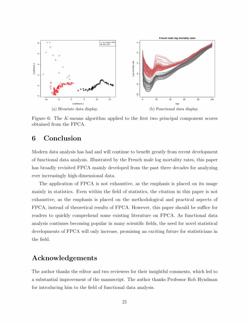
Figure 6a plots two clusters obtained by applying the K-means algorithms to the

bivariate principal component scores. The red triangles represent the years at or before

1945, while the black circles represent the years after 1945. From this data set, it indicates

a possible structural change in the French male log mortality rates before and after 1945.

The corresponding indexes of the bivariate principal component scores are matched back

to the functional curves in Figure 6b.

20

−10 −5 0 5 10 15

−2

02

46

8

Coefficient 1

Coe

ffici

ent 2

at or before 1945after 1945

(a) Bivariate data display.

0 20 40 60 80 100

−10

−8

−6

−4

−2

0

French male log mortality rates

Age

Log

mor

talit

y ra

te

(b) Functional data display.

Figure 6: The K-means algorithm applied to the first two principal component scoresobtained from the FPCA.

6 Conclusion

Modern data analysis has had and will continue to benefit greatly from recent development

of functional data analysis. Illustrated by the French male log mortality rates, this paper

has broadly revisited FPCA mainly developed from the past three decades for analyzing

ever increasingly high-dimensional data.

The application of FPCA is not exhaustive, as the emphasis is placed on its usage

mainly in statistics. Even within the field of statistics, the citation in this paper is not

exhaustive, as the emphasis is placed on the methodological and practical aspects of

FPCA, instead of theoretical results of FPCA. However, this paper should be suffice for

readers to quickly comprehend some existing literature on FPCA. As functional data

analysis continues becoming popular in many scientific fields, the need for novel statistical

developments of FPCA will only increase, promising an exciting future for statisticians in

the field.

Acknowledgements

The author thanks the editor and two reviewers for their insightful comments, which led to

a substantial improvement of the manuscript. The author thanks Professor Rob Hyndman

for introducing him to the field of functional data analysis.

21

References

Aggarwal, C. C., Hinneburg, A. & Keim, D. A. (2001), On the surprising behavior of

distance metrics in high dimensional space, in J. Van den Bussche & V. Vianu, eds,

‘Lecture Notes in Computer Science’, Springer-Verlag, London, pp. 420–434.

Aguilera, A. M., Gutierrez, R. & Valderrama, M. J. (1996), ‘Approximation of estimators

in the PCA of a stochastic process using B-splines’, Communications in Statistics —

Simulation and Computation 25(3), 671–690.

Akhiezer, N. I. & Glazman, I. M. (1981), Theory of Linear Operators in Hilbert Space,

Vol. I, Pitman Advanced Publishing Program, Boston, MA.

Aneiros-Perez, G. & Vieu, P. (2008), ‘Nonparametric time series prediction: a semi-

functional partial linear modeling’, Journal of Multivariate Analysis 99(5), 834–857.

Arabie, P. & Hubert, L. (1994), Cluster analysis in marketing research, in ‘Advanced

Methods of Marketing Research’, Cambridge, Blackwell Business, pp. 160–189.

Araki, Y., Konishi, S., Kawano, S. & Matsui, H. (2009), ‘Functional regression modeling via

regularized Gaussian basis expansions’, Annals of the Institute of Statistical Mathematics

61(4), 811–833.

Aston, J. A. D., Chiou, J.-M. & Evans, J. (2010), ‘Linguistic pitch analysis using functional

principal component mixed effect models’, Journal of the Royal Statistical Society (Series

C) 59(2), 297–317.

Bali, J. L., Boente, G., Tyler, D. E. & Wang, J.-L. (2011), ‘Robust functional principal

components: a projection-pursuit approach’, Annals of Statistics 39(6), 2852–2882.

Bathia, N., Yao, Q. & Ziegelmann, F. (2010), ‘Identifying the finite dimensionality of curve

time series’, The Annals of Statistics 38(6), 3352–3386.

Bellman, R. E. (1961), Adaptive Control Processes: a Guided Tour, Princeton University

Press, Princeton, New Jersey.

Benko, M. & Hardle, W. (2005), Common functional implied volatility analysis, in P. Cizek,

W. Hardle & R. Weron, eds, ‘Statistical Tools for Finance and Insurance’, Springer,

Berlin, pp. 115–134.

22

Benko, M., Hardle, W. & Kneip, A. (2009), ‘Common functional principal components’,

The Annals of Statistics 37(1), 1–34.

Besse, P. (1992), ‘PCA stability and choice of dimensionality’, Statistics and Probability

Letters 13(5), 405–410.

Boente, G., Rodriguez, D. & Sued, M. (2010), ‘Inference under functional proportional and

common principal component models’, Journal of Multivariate Analysis 101(2), 464–475.

Bosq, D. (2000), Linear Processes in Function Spaces: Theory and Applications, Springer,

New York.

Bouveyron, C. & Jacques, J. (2011), ‘Model-based clustering of time series in group-specific

functional subspaces’, Advances in Data Analysis and Classification 5(4), 281–300.

Cardot, H., Faivre, R. & Goulard, M. (2003), ‘Functional approaches for predicting land

use with the temporal evolution of coarse resolution remote sensing data’, Journal of

Applied Statistics 30(10), 1185–1199.

Cardot, H., Ferraty, F., Mas, A. & Sarda, P. (2003), ‘Testing hypotheses in the functional

linear model’, Scandinavian Journal of Statistics 30(1), 241–255.

Cardot, H., Ferraty, F. & Sarda, P. (1999), ‘Functional linear model’, Statistics & Probability

Letters 45(1), 11–22.

Cardot, H., Mas, A. & Sarda, P. (2007), ‘CLT in functional linear regression models’,

Probability Theory and Related Fields 138(3-4), 325–361.

Castro, P. E., Lawton, W. H. & Sylvestre, E. A. (1986), ‘Principal modes of variation for

processes with continuous sample curves’, Technometrics 28(4), 329–337.

Cattell, R. B. (1966), ‘The scree test for the number of factors’, Multivariate Behavioral

Research 1(2), 245–276.

Chiou, J.-M. & Muller, H.-G. (2009), ‘Modeling hazard rates as functional data for the

analysis of cohort lifetables and mortality forecasting’, Journal of the American Statistical

Association 104(486), 572–585.

23

Chiou, J.-M., Muller, H.-G. & Wang, J.-L. (2003), ‘Functional quasi-likelihood regression

models with smooth random effects’, Journal of the Royal Statistical Society: Series B

65(2), 405–423.

Chiou, J.-M., Muller, H.-G. & Wang, J.-L. (2004), ‘Functional response models’, Statistica

Sinica 14(3), 659–677.

Chiou, J.-M., Muller, H.-G., Wang, J.-L. & Carey, J. R. (2003), ‘A functional multiplicative

effects model for longitudinal data, with application to reproductive histories of female

medflies’, Statistica Sinica 13(4), 1119–1133.

Coffey, N., Harrison, A. J., Donoghue, O. A. & Hayes, K. (2011), ‘Common functional

principal components analysis: a new approach to analyzing human movement data’,

Human Movement Science 30(6), 1144–1166.

Crainiceanu, C. M., Staicu, A.-M. & Di, C.-Z. (2009), ‘Generalized multilevel functional

regression’, Journal of the American Statistical Association 104(488), 1550–1561.

Cuesta-Albertos, J. A. & Nieto-Reyes, A. (2010), Functional classification and the random

Tukey depth. Practical issues, in C. Borgelt, G. G. Rodriguez, W. Trutschnig, M. A.

Lubiano, M. Gil, P. Grzegorzewski & O. Hryniewicz, eds, ‘Combining Soft Computing

and Statistical Methods in Data Analysis. Advances in Intelligent and Soft Computing’,

Vol. 77, Springer, pp. 123–130.

Cuevas, A., Febrero, M. & Fraiman, R. (2002), ‘Linear functional regression: the case

of fixed design and functional response’, The Canadian Journal of Statistics/La Revue

Canadienne de Statistique 30(2), 285–300.

Cuevas, A., Febrero, M. & Fraiman, R. (2007), ‘Robust estimation and classification for

functional data via projection-based depth notions’, Computational Statistics 22(3), 481–

496.

Cuevas, A. & Fraiman, R. (2009), ‘On depth measures and dual statistics. A methodology

for dealing with general data’, Journal of Multivariate Analysis 100(4), 753–766.

Dauxois, J., Pousse, A. & Romain, Y. (1982), ‘Asymptotic theory for the principal compo-

nent analysis of a vector random function: some applications to statistical inference’,

Journal of Multivariate Analysis 12(1), 136–154.

24

Davidian, M., Lin, X. & Wang, J.-L. (2004), ‘Introduction: emerging issues in longitudinal

and functional data analysis’, Statistica Sinica 14(3), 613–614.

Delaigle, A. & Hall, P. (2012), ‘Achieving near perfect classification for functional data’,

Journal of the Royal Statistical Society, Series B 74(2), 267–286.

Delaigle, A., Hall, P. & Bathia, N. (2012), ‘Componentwise classification and clustering of

functional data’, Biometrika 99(2), 299–313.

Di, C.-Z., Crainiceanu, C. M., Caffo, B. S. & Punjabi, N. M. (2009), ‘Multilevel functional

principal component analysis’, The Annals of Applied Statistics 3(1), 458–488.

Eilers, P. H. C. & Marx, B. D. (1996), ‘Flexible smoothing with B-splines and penalties

(with discussion)’, Statistical Science 11(2), 89–121.

Fan, Y. & James, G. (2013), Functional additive regression, Working paper, University of

Southern California.

URL: http://www-bcf.usc.edu/~gareth/research/FAR.pdf

Faraway, J. J. (1997), ‘Regression analysis for a functional response’, Technometrics

39(3), 254–261.

Febrero-Bande, M. & Gonzalez-Manteiga, W. (2011), Generalized additive models for

functional data, in F. Ferraty, ed., ‘Recent Advances in Functional Data Analysis and

Related Topics’, Contributions to Statistics, Springer, Heidelberg.

Fengler, M. R., Hardle, W. K. & Villa, C. (2003), ‘The dynamics of implied volatilities: a

common principal components approach’, Review of Derivatives Research 6(3), 179–202.

Ferraty, F., Goia, A., Salinelli, E. & Vieu, P. (2011), Recent advances on functional additive

regression, in F. Ferraty, ed., ‘Recent Advances in Functional Data Analysis and Related

Topics’, Springer, Heidelberg, pp. 97–102.

Ferraty, F. & Romain, Y., eds (2011), The Oxford Handbook of Functional Data Analysis,

Oxford University Press, Oxford.

Ferraty, F. & Vieu, P. (2006), Nonparametric Functional Data Analysis: Theory and

Practice, Springer, New York.

25

Foutz, N. & Jank, W. (2010), ‘Pre-release demand forecasting for motion pictures using

functional shape analysis of virtual stock markets’, Marketing Science 29(3), 568–579.

Fraiman, R. & Muniz, G. (2001), ‘Trimmed means for functional data’, TEST 10(2), 419–

440.

Geenens, G. (2011), ‘Curse of dimensionality and related issues in nonparametric functional

regression’, Statistics Surveys 5, 30–43.

Gervini, D. (2008), ‘Robust functional estimation using the median and spherical principal

components’, Biometrika 95(3), 587–600.

Gervini, D. (2012), ‘Outlier detection and trimmed estimation for general functional data’,

Statistica Sinica 22(4), 1639–1660.

Glendinning, R. H. & Herbert, R. A. (2003), ‘Shape classification using smooth principal

components’, Pattern recognition letters 24(12), 2021–2030.

Gonzalez-Manteiga, W. & Vieu, P. (2007), ‘Statistics for functional data (editorial)’,

Computational Statistics & Data Analysis 51(10), 4788–4792.

Green, P. J. & Silverman, B. W. (1994), Nonparametric Regression and Generalized Linear

Models: a Roughness Penalty Approach, Chapman & Hall, London.

Hall, P. (2011), Principal component analysis for functional data: methodology, theory and

discussion, in ‘The Oxford Handbook of Functional Data Analysis’, Oxford University

Press, pp. 210–234.

Hall, P. & Horowitz, J. L. (2007), ‘Methodology and convergence rates for functional linear

regression’, The Annals of Statistics 35(1), 70–91.

Hall, P. & Hosseini-Nasab, M. (2006), ‘On properties of functional principal components

analysis’, Journal of the Royal Statistical Society: Series B 68(1), 109–126.

Hall, P., Muller, H.-G. & Wang, J.-L. (2006), ‘Properties of principal component methods

for functional and longitudinal data analysis’, The Annals of Statistics 34(3), 1493–1517.

Hall, P., Poskitt, D. S. & Presnell, B. (2001), ‘A functional data-analytic approach to

signal discrimination’, Technometrics 43(1), 1–9.

26

Hall, P. & Vial, C. (2006), ‘Assessing the finite dimensionality of functional data’, Journal

of the Royal Statistical Society (Series B) 68(4), 689–705.

Harezlak, J., Coull, B. A., Laird, N. M., Magari, S. R. & Christiani, D. C. (2007), ‘Penalized

solutions to functional regression problems’, Computational Statistics & Data Analysis

51(10), 4911–4925.

Hartigan, J. A. & Wong, M. A. (1979), ‘Algorithm AS 136: a K-means clustering algorithm’,

Journal of the Royal Statistical Society, Series C 28(1), 100–108.

Hastie, T., Buja, A. & Tibshirani, R. (1995), ‘Penalized discriminant analysis’, The Annals

of Statistics 23(1), 73–102.

Hlubinka, D. & Prchal, L. (2007), ‘Changes in atmospheric radiation from the statistical

point of view’, Computational Statistics & Data Analysis 51(10), 4926–4941.

Hoerl, A. E. (1962), ‘Application of ridge analysis to regression problems’, Chemical

Engineering Progress 58(3), 54–59.

Horvath, L. & Kokoszka, P. (2012), Inference for Functional Data with Applications,

Springer, New York.

Horvath, L. & Reeder, R. (2011), A test of significance in functional quadratic regression,

Working paper, University of Utah.

URL: http://arxiv.org/pdf/1105.0014v1.pdf

Huang, D.-S. & Zheng, C.-H. (2006), ‘Independent component analysis-based penalized

discriminant method for tumor classification using gene-expression data’, Bioinformatics

22(15), 1855–1862.

Human Mortality Database (2012), University of California, Berkeley (USA), and Max

Planck Institute for Demographic Research (Germany). Accessed at 8/3/2012.

URL: http://www.mortality.org/

Hyndman, R. J. (1996), ‘Computing and graphing highest density regions’, The American

Statistician 50(2), 120–126.

Hyndman, R. J., Koehler, A. B., Ord, J. K. & Snyder, R. D. (2008), Forecasting with

Exponential Smoothing: the State Space Approach, Springer, Berlin.

27

Hyndman, R. J. & Shang, H. L. (2009), ‘Forecasting functional time series (with discussion)’,

Journal of the Korean Statistical Society 38(3), 199–221.

Hyndman, R. J. & Shang, H. L. (2010), ‘Rainbow plots, bagplots, and boxplots for

functional data’, Journal of Computational and Graphical Statistics 19(1), 29–45.

Hyndman, R. J. & Ullah, M. S. (2007), ‘Robust forecasting of mortality and fertility rates: a

functional data approach’, Computational Statistics & Data Analysis 51(10), 4942–4956.

Illian, J. B., Prosser, J. I., Baker, K. L. & Rangel-Castro, J. I. (2009), ‘Functional principal

component data analysis: a new method for analysing microbial community fingerprints’,

Journal of Microbiological Methods 79(1), 89–95.

James, G. M. (2002), ‘Generalized linear models with functional predictors’, Journal of the

Royal Statistical Society: Series B 64(3), 411–432.

James, G. M. & Hastie, T. J. (2001), ‘Functional linear discriminant analysis for irregularly

sampled curves’, Journal of the Royal Statistical Society: Series B 63(3), 533–550.

James, G. M., Hastie, T. J. & Sugar, C. A. (2000), ‘Principal component models for sparse

functional data’, Biometrika 87(3), 587–602.

James, G. M. & Silverman, B. W. (2005), ‘Functional adaptive model estimation’, Journal

of the American Statistical Association 100(470), 565–576.

James, G. M. & Sugar, C. A. (2003), ‘Clustering for sparsely sampled functional data’,

Journal of the American Statistical Association 98(462), 397–408.

Jank, W. & Yahav, I. (2010), ‘E-loyalty networks in online auctions’, Annals of Applied

Statistics 4(1), 151–178.

Jones, M. C. & Rice, J. A. (1992), ‘Displaying the important features of large collections

of similar curves’, The American Statistician 46(2), 140–145.

Karhunen, K. (1946), ‘Zur spektraltheorie stochastischer prozesse’, Annales Academiae

Scientiarum Fennicae 37, 1–37.

28

Kayano, M. & Konishi, S. (2010), ‘Sparse functional principal component analysis via regu-

larized basis expansions and its application’, Communications in Statistics - Simulation

and Computation 39(7), 1318–1333.

Kramer, N., Boulesteix, A.-L. & Tutz, G. (2008), ‘Penalized partial least squares with appli-

cations to B-spline transformations and functional data’, Chemometrics and Intelligent

Laboratory Systems 94(1), 60–69.

Lee, H.-J. (2004), Functional data analysis: classification and regression, PhD thesis, Texas

A & M University.

URL: http://repository.tamu.edu/handle/1969.1/2805

Locantore, N., Marron, J. S., Simpson, D. G., Tripoli, N., Zhang, J. T. & Cohen, K. L.

(1999), ‘Robust principal component analysis for functional data’, Test 8(1), 1–73.

Loeve, M. (1946), ‘Fonctions aleatoires a decomposition orthogonale exponentielle’, La

Revue Scientifique 84, 159–162.

Lopez-Pintado, S. & Romo, J. (2007), ‘Depth-based inference for functional data’, Compu-

tational Statistics & Data Analysis 51(10), 4957–4968.

Lopez-Pintado, S. & Romo, J. (2009), ‘On the concept of depth for functional data’, Journal

of the American Statistical Association 104(486), 718–734.

Mas, A. (2002), ‘Weak convergence for the covariance operators of a Hilbertian linear

process’, Stochastic processes and their applications 99(1), 117–135.

Mas, A. (2008), ‘Local functional principal component analysis’, Complex Analysis and

Operator Theory 2(1), 135–167.

Mas, A. & Pumo, B. (2007), ‘The ARHD model’, Journal of Statistical Planning and

Inference 137(2), 538–553.

Mas, A. & Pumo, B. (2009), ‘Functional linear regression with derivatives’, Journal of

Nonparametric Statistics 21(1), 19–40.

Matsui, H., Araki, Y. & Konishi, S. (2008), ‘Multivariate regression modeling for functional

data’, Journal of Data Science 6(3), 313–331.

29

Muller, H.-G. & Stadtmuller, U. (2005), ‘Generalized functional linear models’, The Annals

of Statistics 33(2), 774–805.

Muller, H.-G. & Yao, F. (2010), ‘Additive modelling of functional gradients’, Biometrika

97(4), 791–805.

Muller, H. & Yao, F. (2008), ‘Functional additive models’, Journal of the American

Statistical Association 103(484), 1534–1544.

Pezzulli, S. & Silverman, B. W. (1993), ‘Some properties of smoothed principal components

analysis for functional data’, Computational Statistics 8, 1–16.

Poskitt, D. S. & Sengarapillai, A. (2013), ‘Description length and dimensionality reduction

in functional data analysis’, Computational Statistics and Data Analysis 58(2), 98–113.

Preda, C. & Saporta, G. (2005), ‘PLS regression on a stochastic process’, Computational

Statistics & Data Analysis 48(1), 149–158.

Preda, C., Saporta, G. & Leveder, C. (2007), ‘PLS classification of functional data’,

Computational Statistics 22(2), 223–235.

Ramsay, J. O. (1988), ‘Monotone regression splines in action’, Statistical Science 3(4), 425–

441.

Ramsay, J. O. (2000), ‘Functional components of variation in handwriting’, Journal of the

American Statistical Association 95(449), 9–15.

Ramsay, J. O. & Dalzell, C. J. (1991), ‘Some tools for functional data analysis (with

discussion)’, Journal of the Royal Statistical Society: Series B 53(3), 539–572.

Ramsay, J. O. & Silverman, B. W. (1997), Functional Data Analysis, Springer, New York.

Ramsay, J. O. & Silverman, B. W. (2002), Applied Functional Data Analysis: Methods and

Case Studies, Springer, New York.

Ramsay, J. O. & Silverman, B. W. (2005), Functional Data Analysis, 2nd edn, Springer,

New York.

Rao, C. R. (1958), ‘Some statistical methods for comparison of growth curves’, Biometrics

14(1), 1–17.

30

Reiss, P. T. & Ogden, R. T. (2007), ‘Functional principal component regression and func-

tional partial least squares’, Journal of the American Statistical Association 102(479), 984–

996.

Rice, J. A. (2004), ‘Functional and longitudinal data analysis: perspectives on smoothing’,

Statistica Sinica 14(3), 631–647.

Rice, J. A. & Silverman, B. W. (1991), ‘Estimating the mean and covariance structure

nonparametrically when the data are curves’, Journal of the Royal Statistical Society:

Series B 53(1), 233–243.

Rice, J. & Wu, C. (2001), ‘Nonparametric mixed effects models for unequally sampled

noisy curves’, Biometrics 57(1), 253–259.

Rossi, F., Conan-Guez, B. & El Golli, A. (2004), Clustering functional data with the SOM

algorithm, in ‘European Symposium on Artificial Neural Networks’, pp. 305–312.

Rousseeuw, P. J., Ruts, I. & Tukey, J. W. (1999), ‘The bagplot: a bivariate boxplot’, The

American Statistician 53(4), 382–387.

Scott, D. W. (1992), Multivariate Density Estimation: Theory, Practice, and Visualization,

Wiley, New York.

Shang, H. L. & Hyndman, R. J. (2011), ‘Nonparametric time series forecasting with

dynamic updating’, Mathematics and Computers in Simulation 81(7), 1310–1324.

Shen, H. (2009), ‘On modeling and forecasting time series of smooth curves’, Technometrics

51(3), 227–238.

Shibata, R. (1981), ‘An optimal selection of regression variables’, Biometrika 68(1), 45–54.

Silverman, B. W. (1996), ‘Smoothed functional principal components analysis by choice of

norm’, The Annals of Statistics 24(1), 1–24.

Song, J. J., Deng, W., Lee, H.-J. & Kwon, D. (2008), ‘Optimal classification for time-

course gene expression data using functional data analysis’, Computational Biology and

Chemistry 32(6), 426–432.

31

Sood, A., James, G. M. & Tellis, G. J. (2009), ‘Functional regression: a new model for

predicting market penetration of new products’, Marketing Science 28(1), 36–51.

Suyundykov, R., Puechmorel, S. & Ferre, L. (2010), Multivariate functional data clusteriza-

tion by PCA in Sobolev space using wavelets, Technical report, University of Toulouse.

URL: http://hal.inria.fr/docs/00/49/47/02/PDF/p41.pdf

Tarpey, T. (2007), ‘Linear transformations and the k-means clustering algorithm: applica-

tions to clustering curves’, The American Statistician 61(1), 34–40.

Tran, N. M. (2008), An introduction to theoretical properties of functional principal

component analysis, Honours thesis, The University of Melbourne.

URL: http://www.stat.berkeley.edu/~tran/pub/honours_thesis.pdf

Tu, I.-P., Chen, H. & Chen, X. (2009), ‘An eigenvector variability plot’, Statistica Sinica

19(4), 1741–1754.

Tucker, L. R. (1958), ‘Determination of parameters of a functional relation by factor

analysis’, Psychometrika 23(1), 19–23.

Tukey, J. W. (1975), Mathematics and the picturing of data, in R. D. James, ed., ‘Proceed-

ings of the International Congress of Mathematicians’, Vol. 2, Canadian mathematical

congress, Aug. 21-29, 1974, Vancouver, pp. 523–531.

Valderrama, M. J. (2007), ‘An overview to modelling functional data (editorial)’, Compu-

tational Statistics 22(3), 331–334.

Wahba, G. (1990), Spline Models for Observational Data, Society for Industrial and Applied

Mathematics, Philadelphia.

Weidmann, J. (1980), Linear Operators in Hilbert Spaces, Springer-Verlag, New York.

Yamamoto, M. (2012), ‘Clustering of functional data in a low-dimensional subspace’,

Advances in Data Analysis and Classification 6(3), 219–247.

Yao, F., Fu, Y. & Lee, T. C. M. (2011), ‘Functional mixture regression’, Biostatistics

12(2), 341–353.

32

Yao, F. & Lee, T. C. M. (2006), ‘Penalized spline models for functional principal component

analysis’, Journal of the Royal Statistical Society: Series B 68(1), 3–25.

Yao, F. & Muller, H.-G. (2010), ‘Functional quadratic regression’, Biometrika 97(1), 49–64.

Yao, F., Muller, H.-G. & Wang, J.-L. (2005a), ‘Functional data analysis for sparse longitu-

dinal data’, Journal of the American Statistical Association 100(470), 577–590.

Yao, F., Muller, H.-G. & Wang, J.-L. (2005b), ‘Functional linear regression analysis for

longitudinal data’, The Annals of Statistics 33(6), 2873–2903.

Zhou, L., Huang, J. Z. & Carroll, R. J. (2008), ‘Joint modelling of paired sparse functional

data using principal components’, Biometrika 95(3), 601–619.

Zipunnikov, V., Caffo, B., Yousem, D. M., Davatzikos, C., Schwartz, B. S. & Crainiceanu,

C. (2011), ‘Multilevel functional principal component analysis for high-dimensional data’,

Journal of Computational and Graphical Statistics 20(4), 852–873.

33