a survey on rainfall prediction techniques

International Journal of Computer Application (2250-1797)

Volume 6– No.2, March- April 2016

28

A Survey On Rainfall Prediction Techniques

MR. DHAWAL HIRANI #1

, DR. NITIN MISHRA#2

Keywords:Rainfall,NN,BPN,RBF,SVM,SOM,ANN,ARIMA,ASTAR,MLR,WRF,GFS

INTRODUCTION: Agriculture is the backbone of Indian economy. Irrigation facility is

still not so good in India and most of agriculture depends upon the rain. A good rainfall

result in the occurrence of a dry period for a long time or heavy rain both affect the crop

yield as well as the economy of country, so due to that early prediction of rainfall is

very crucial . A wide range of rainfall forecast methods are employed in weather

prediction at regional and national levels. Fundamentally there are two approaches to

predict Rainfall. They are Empirical and Dynamical Methods.

The Empirical approach is

based on analysis of past historical data of weather and its relationship to a variety of

atmospheric variables over different parts of Chhattisgarh. The most widely use empirical

approaches used for climate prediction are Regression, artificial neural network, fuzzy

logic and group method of data handling.

The dynamical approach, predictions are

generated by physical models based on system of equations that predict the future Rainfall.

The forecasting of weather by computer using equations are known as numerical weather

prediction. To predict the weather by numeric means, meteorologist has develop atmospheric

models that approximate the change in temperature, pressure etc using mathematical

equations.

DIFFERENT METHODS OF RAINFALL PREDICTION :

MULTIPLE LINEAR REGRESSION

Regression is a statistical measure that attempts to determine the strength of the relationship between one dependent variable usually denoted by Y and a series of other changing variables known as independent variables. Regression model which contain more than two predictor variables are called Multiple Regression Model.

#1 MTECH SCHOLAR COMPUTER TECHNOLOGY, RCET, BHILAI (C.G) INDIA, 9977426319.

#2 ASSOCIATE PROFESSOR, CSE DEPARTMENT, RCET, BHILAI (C.G) INDIA, 9685240263.

ABSTRACT: India is an agricultural country and most of economy of India depends upon the

agriculture. Rainfall plays an important role in agriculture so early prediction of rainfall is necessary

for the better economic growth of our country. Rainfall prediction has been the one of the most

challenging issue around the world in last year. Widely used techniques for prediction are

Regression analysis, clustering, and Artificial Neural Network (ANN) etc. This paper represents a

review of different rainfall prediction techniques for the early prediction of rainfall prediction of

rainfall



29

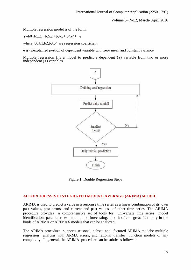
Multiple regression model is of the form: Y=b0+b1x1 +b2x2 +b3x3+ b4x4+...e where b0,b1,b2,b3,b4 are regression coefficient e is unexplained portion of dependent variable with zero mean and constant variance. Multiple regression fits a model to predict a dependent (Y) variable from two or more independent (X) variables

Figure 1. Double Regression Steps

AUTOREGRESSIVE INTEGRATED MOVING AVERAGE (ARIMA) MODEL

ARIMA is used to predict a value in a response time series as a linear combination of its own

past values, past errors, and current and past values of other time series. The ARIMA

procedure provides a comprehensive set of tools for uni-variate time series model

identification, parameter estimation, and forecasting, and it offers great flexibility in the

kinds of ARIMA or ARIMAX models that can be analyzed.

The ARIMA procedure supports seasonal, subset, and factored ARIMA models; multiple

regression analysis with ARMA errors; and rational transfer function models of any

complexity. In general, the ARIMA procedure can be subtle as follows :



30

Step 0) A class of models is formulated assuming certain hypotheses

In this step, a general ARIMA formulation is selected to model the rain fall data. This

selection is carried out by careful inspection and selection of the main characteristic of the

daily rain fall and other meteorological data.The corresponding data are: humidity, air

pressure, surface land temperature and wind velocity (corresponding to daily respectively),

among others.

Step 1) A model is identified for the observed data.

A trial model must be identified for the rain fall data. First, in order to make the underlying

process stationary (a more homogeneous mean and variance), a transformation of the

original rain fall data and the inclusion offactors of the form trial model must be identified

for the rain fall data. First, in order to make the underlying process stationary (a more

homogeneous mean and variance), a transformation of the original rain fall data and the

inclusion offactors of the form may be necessary. In this step, the checking process can

be done using Autocorrelationfunction (ACF) or unit root test. A further check for lag

residual and lag dependent tested from partial ACF.

Step 2) The model parameters are estimated.

After the functions of the model have been specified, the parameters of these functions

must be estimated. Good estimators of the parameters can be computed by assuming the

data are observations of a stationary time series (Step 1). If a Moving Average (MA)

pattern is identified then further optimization process needed by using maximum likelihood

or least square estimation.

A conditional likelihood function is selected in order to get a good starting point to obtain an

exact likelihoodfunction. Also, an option to detect and adjust possible unusual observations

is selected. As these events are notinitially known, a procedure that detects and

minimizes the effect of the outliers is necessary. With this adjustment, a better

understanding of the series, a better modeling and estimation, and, finally, a better

forecasting performance is achieved.

Step 3) If the hypotheses of the model are validated, go to Step 4, otherwise go to Step 1 to

refine the model.

In this step, a diagnosis check is used to validate the model assumptions of Step 0. This

diagnosis checks if the hypotheses made on the residuals (actual prices minus fitted

prices, as estimated in Step 1) are true. Residuals must satisfy the requirements of a

white noise process: zero mean, constant variance, uncorrelated process and normal

distribution. These requirements can be checked by taking tests for randomness, such as the

autocorrelation and partial autocorrelation plots. If the hypotheses on the residuals are

validated by tests and plots, then, the model can be used to forecast prices. Otherwise, the

residuals contain a certain structure that should be studied to refine the model in Step 1.

Step 4) The model is ready for forecasting.

In Step 4, the model from Step 2 can be used to predict future values of daily rainfall



31

data. Due to this requirement, difficulties may arise because predictions can be less

certain as the forecast lead time becomes larger. Based on the natural of data, time series

forecasting is suit to short term forecasting (hourly or daily). For a long term period, a

structural forecaster is more comply for the situation.

The flowchart of corresponding steps above can be seen in Fig. below

Figure 2. ARIMA Process

GENETIC ALGORITHM

Genetic algorithms are algorithms that attempt to apply an understanding of the natural

evolution in problem-solving tasks (problem solving). The approach taken by this algorithm

is to combine a wide selection of solutions randomly within a population and then evaluate

them to get the best solution By doing this process repeatedly, these algorithms simulate the

process of evolution as the desired number of generations. This generation will represent

improvements on previous population. In the end, we will get the best solutions appropriate

to the problems faced. To use a genetic algorithm, solutions to problems represented as a set

of genes that make up chromosomes. This chromosome was randomly based coding

techniques are used. The entire set of chromosomes is observed representative of the

population.

Chromosomes will be evolved in several stages iterations called generations. The new

generation is obtained By cross breeding techniques (crossover) and mutation (mutation).

Crossover includes cutting two pieces of chromosomes based on the desired number of

points and then combine half of each chromosome with other couples. While mutations

include the replacement value of the gene in a chromosome with the value of other genes

from other chromosomes become partner. The chromosomes are then evolved to a

suitability criterion (fitness) and the set will be selected the best results while others are

ignored. Furthermore, the process repeated until you have a chromosome that has the best fit

(best fitness) to be taken as the best solution of the problem. On Genetic Algorithms, the best

1963



32

solution search techniques performed simultaneously at a number of solutions known as

population. Individuals in a population are referred to as chromosomes. This chromosome is

a solution that is shaped symbol. Initial population is built randomly, while the next

population is the result of the evolution of chromosomes through iterations called

generations. In each generation, the chromosomes will go through an evaluation process

using a measurement tool called the fitness function. Fitness value of a chromosome will

show the quality of the chromosomes in the population.

The next generation is known as the child (offspring) are formed from the combination of

two generations of chromosomes that act as the parent (parent) using the crossover

operator. Besides crossover operator, achromosome can also be modified by using

mutation operators. The population of the new generation is formed by selecting the fitness

value of parent chromosome and the fitness value of the chromosomes of children, and

discard the other chromosomes so that the population size (the number of chromosomes in a

population) constant. After several generations, the algorithm will converge to the best

chromosome.

Genetic Algorithms steps for generating initial weight as follows:

1.Create an initial population randomly of meteorological data.

2. Evaluate each individual in the population.

3.Generate new population using genetic operations.

4.Determine the final result at the time of termination criteria.

ADAPTIVE SPLINES THRESHOLD AUTOREGRESSIVE (ASTAR) Modelling

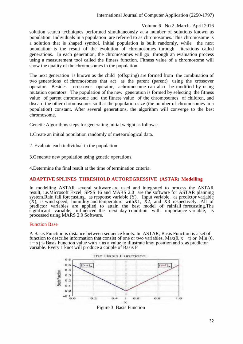
In modelling ASTAR several software are used and integrated to process the ASTAR result, i.e.Microsoft Excel, SPSS 16 and MARS 2.0 are the software for ASTAR planning system.Rain fall forecasting, as response variable (Y), Input variable, as predictor variable (X), is wind speed, humidity and temperature withX1, X2, and X3 respectively. All of predictor variables are applied to attain the best model of rainfall forecasting.The significant variable, influenced the next day condition with importance variable, is processed using MARS 2.0 Software. Function Base A Basis Function is distance between sequence knots. In ASTAR, Basis Function is a set of function to describe information that consist of one or two variables. Max(0, x − t) or Min (0, t − x) is Basis Function value with t as a value to illustrate knot position and x as predictor variable. Every 1 knot will produce a couple of Basis F Figure 3. Basis Function



33

ASTAR Methods as data analysis technique to find the best model from a set of data. It is using past and present data to predict the short-term forecasting.

Modelling Stage of ASTAR

1.Determine maximum Basis Function, maximum interaction numbers and minimum

observation numbers between knots.

2.Forward Stepwise Processing to obtain maximum number of Basis Function using MARS

2.0

3.Backward Stepwise Processing to obtain Basis Function numbers from forward stepwise

by minimizing the least GCV (Generalized Cross Validation) value.

4.Knots selection using forward and backward algorithm.

5.Estimating the coefficient of chosen Basis Function as a stage of response variable (Y)

prediction (Y) to predictor variable (X).

Figure 4 . Flowchart of ASTAR Methodology

SUPPORT VECTOR MACHINE (SVM)

A Support Vector Machine (SVM) is a computer algorithm that learns by example to find the best function of classifier hyperplane to separate the two classes in the Input space.The SVM analyzed two kinds of data, i.e. linearly and non- linearly separable data .The example of linearly separated data is shown in fig. below. Best hyperplane between



34

two classes can be foundby measuring the hyperplanemargin and find out the maximum points.Margin is defined as the distance between hyperplane and the closest pattern of each class, which is called support vector.The best hyperplane is defined by the following equation f(x) = w x+ b(1)

T Where x refers to a training pattern, w is referred to as the weight vector and b as the bias term Support vectors f(x) = 0 Margins Figure 5. The example of linearly separated data Support Vector Machine is one of the important category of perceptrons and radial basis function networks, support vector machines can be used for pattern classification and nonlinear regression. Support Vector Machines (SVMs) developed by Vapnik and his co-workers has been used for supervised learning due to – (i) Better generalization performance than other NN models (ii) Solution of SVM is unique, optimal and absent from local minima as it uses linearly constrained quadratic programming problem (iii) Applicability to non- vectorial data (Strings and Graphs) and (iv) Few parameters are required for tuning the learning m/c. Kernel Methods are a set of algorithms from statistical learning which include the SVM for classification and regression, Kernel PCA, Kernel based clustering, feature selection, and dimensionality reduction etc . SVM is found to be a significant technique to solve many classifications problem in the last couple of years. Very few researchers of this field used this technique for rainfall prediction and got satisfactory result. FUZZY LOGIC (FUZZY)

Fuzzy Logic is a type of reasoning based on the recognition that logical statements are not only true or false (white or black areas of probability) but can also range from “almost certain” to “very unlikely”.Fuzzy logic has proven to be particularly useful in expert system applications. Fuzzy inference system is shown in diagram below. They are composed of five conventional blocks a rule-base containing a number of fuzzy if-then rules, a database which defines the membership functions of the fuzzy sets used in the fuzzy rules, a decision making unit which performs the inference operations on the rules, a fuzzification interface which transform the crisp inputs into degrees of match with linguistic values, a defuzzification interface which transform the fuzzy results of the inference into a crisp output.



35

INTERFACE

Figure 6. The general structure of Fuzzy Inference System BACK-PROPAGATION NEURAL NETWORK(BPNN)

In 1980’s the idea of Artificial Neural network first sprang up. As ANN has the ability to solve complex, nonlinear problems, researchers in various fields started using ANN for prediction and forecasting purpose. D.L.Rumelheart etc in California university proposed BP algorithm to reduce the error in the network. BP gets automatically adopted in the parallel structure of ANN which includes input layer, hidden layer and output layer. In each of these layers there are present numerous Processing elements are called neurons which interconnected with each other, however the neurons present in each layer is connected with neurons in the corresponding next layers , no jumping of neurons is allowed . This historical data is given as input to the input layer. It Is necessary that the data should be normalized. The reason behind normalizing the input data is, raw data can’t be fed to network as it results in slow learning of data i.e. the rate at which data get learned will slow down. Figure below shows the mathematical model for a single neuron.

Figure 7. The Mathematical Model for a Single Neuron.

KKKKKKKKKkKkKAAS

DATABASE RULEBASE

DEFUZZIFICATION

INTERFACE

INTERFACE

FUZZIFICATION

INTERFACE

DECISION-MAKING UNIT

KNOWLEDGEBASE

I/P O/P



36

The back-propagation learning algorithm is one of the most important developments in neural networks .This networkis still the most popular and most effective model forcomplex, multi layered networks. This learning algorithm is applied to multilayer feed-forward networks consisting of processing elements with continuous differentiable activation functions. The networks associated with back-propagation learning algorithm are also called back-propagation networks (BPNs). It is a supervised learning method. For a given set of training input-output pair, this algorithm provides a procedure for changing the weights in a BPN to classify the given input patterns correctly. The basic concept of this algorithm is, it consists of two passes through the different layers of the network: a forwardpass and a backward pass. In the forward pass, an input vector is applied to the sensory nodes of the network and its effect propagates through the network layer by layer. Finally a set ofoutputs produced as the actual response of the network.During the forward pass the synaptic weights of the networks are all fixed. During the backward pass, on the other hand, the synaptic weights are all adjusted in accordance with an error correction rule. Specifically, the actual response of the network is subtracted from the desired (target) response to produce an error signal. This error signal is then propagated backward through the network, against the direction of synaptic connection. The synaptic weights are adjusted to make the actual response of the network move closer to the desired response in a statistical sense . The typical back-propagation network contains an input layer, an output layer, and at least one hidden layer. The number ofneurons at each layer and the number of hidden layers determine the networks ability on producing accurate outputs for a particular data set. Most of the researchers have been used this network for rainfall prediction. RADIAL BASIS FUNCTION NETWORKS (RBFN) RBF Networks are the class of nonlinear layered feed forward networks. It is a different approach which views the design of neural network as a curve fitting problem in a high dimensional space. The hidden units provide a set of “functions” that constitute an arbitrary “basis” for the input patterns (vectors) when they are expanded to the hidden space, these functions are called radial-basis functions. The construction of a RBF network involves three layers with entirely different roles: the input layer, the only hidden layer, and the output layer .

When a RBF network is used to perform a complex pattern classification task, the problem solved by transforming it into a high dimensional space in a nonlinear manner. RBF networks and MLPs (Multi Layer Perceptrons) are examples of nonlinear layered feed forward networks. They are both universal approximators. However, these two networks differ from each other. An RBF networks has a single hidden layer, whereas an MLP may have one or more hidden layers. The hidden layer of an RBF network is nonlinear and the output layer is linear, where as the hidden and output layers of an MLP are usually all nonlinear . Several researchers have used this network for accurate rainfall prediction and got valuable results.

SELF ORGANIZING MAP (SOM) Self Organizing Map is a special class of artificial neural network. These networks are based on competitive learning. The output neurons of network compete among themselves tobe activated or fired, with the result that only one output neurons is on at any time. This neuron is called winning neuron. The weight vector associate with winning neurons only updated in the scheme “winner takes all”. Based on unsupervised learning which means that no human intervention is needed during the learning and that little need to be known about the characteristics of input data. In SOM the neurons are organized in one or two dimensional lattice. SOM are data visualization technique invented by Prof. Teuvo Kohonen that reduces the dimensions of data through self- organizing neural networks. The way SOM go about reducing dimensions is by producing a map of usually 1-D or 2-Ds, which plot the similarities of the data by grouping similar data items together. So, SOMs accomplish two things, they reduce dimensions & display similarities.



37

WEATHER RESEARCH AND FORECASTING MODEL

The Weather Research and Forecasting (WRF) model is a numerical weather

Prediction (NWP) and atmospheric simulation system desined for both research and

operational applications. The development of WRF has been a multi-agency effort to

build a next-generation forecast model and data assimilation system to advance the

understanding and prediction of weather and accelerate the transfer of research

advances into operations. The geogrid defines model domains and interpolates static

geographical data to the grids. ungrib extracts meteorological fields from GRID formatted

files.The metagrid horizontally interpolates the meteorological fields extracted by by ungrib

tothe model grids defined by geogrid.

Each of the WPS programs reads parameters from a common namelist file, as shown in

the figure.This namelist file has separate namelist records for each of the programs

and a shared namelist record, which defines parameters that are used by more than

one WPS program The ungrib program reads GRIB files degribs the data, and writes the data in a simple

format, called the intermediate format.GRIB (Gridded Binary or General Regularly-

distributed Information in Binary form) is a mathematically concise data format

commonly used in meteorology to store historical and forecast weather data.

Figure 8. WRF Preprocessing System

Static Geographical Data Grided data: NAM, GFS, RUC, AGRMET

geogrid ungrib

metgrid

namelist.wps

real.exe



38

Seasonal Climate Forecasting The CGCM is run by the BoM out for 9 months every day. Forecast products aregenerated from dynamical model output using data analysis software. The resulting derived forecast products are persisted in self describing files with additional metadata to support the clients that deliverthe outlooks. Forecast data is exposed via a data server. Scheduled processes access and reformat the data for SCOPIC (Seasonal climate outlooks for pacific island Countries) access. Custom web services use the data server’s interface to the forecast data to provide maps, data, and line plots. The Pacific Adaptation Strategy Assistance Program (PASAP) Portal consumes the outputs of the custom web services, and displays model based outlooks as overlays on dynamical maps and standard plots.The high predictability of seasonal climate in the tropical Pacific provides opportunities for using seasonal forecasts to improve the resilience of climate sensitive sectors throughout the region. Since 2004 the Pacific Island-Climate Prediction Project (PI-CPP) managed by the Australian Bureau of Meteorology (BoM) has built seasonal prediction capabilities within National Meteorological Services (NMS) of PacificIsland countries through the development and provision of decision support software GLOBAL DATA FORECAST SYSTEM A new Global Forecast System (GFS) has been implemented at Northern Hemisphere Analysis Center of IMD on High Power Computing Systems (HPCS). The new GFS is running in experimental real-time model since 15th January 2010. This new higher resolution global forecast model. The GFS at IMD Delhi involves 4 steps as given below:

Steps 1 - Data Decoding and Quality

Control: First step of the forecast system is data decoding. It runs 48 times in a day on

half-hourly basis, as soon as GTS data files are updated at regional telecom hub (RTH)

of global telecom system (GTS) at IMD New Delhi. Steps 2- Preprocessing of data: (PREPBUFR): Runs 4 times a day at 0000, 0600, 1200 & 1800 UTC. Step 3 - Global Data Assimilation (GDAS) cycle: The Global Data Assimilation cycle runs 4 times a day (00, 06, 12 and 18 UTC).

The assimilation system is a global 3- dimensional variational technique, based on

NCEP’s Grid Point Statistical Interpolation (GSI) scheme, which is the next generation

of Spectral Statistical Interpolation (SSI).

Step 4 – Forecast Integration for 7 days: The analysis and forecast for 7 days is performed using the HPCS installed in IMD Delhi. One GDAS cycle and seven dayforecast (168 hour) run takes about 30 minutes.



39

Figure9. Flow Chart of Global Forecast System

GENERAL DATA MINING RAINFALL PREDICTION MODEL:

In general data mining prediction model first we collect the historical weather data. Data were collected from Indian metrological department pune.the collected data consist ofdifferent features including daily dew point temperature (Celsius), relative humidity, wind speed (KM/H), Station level pressure, Mean sea level, wind speed, pressure and rainfall observation.Creating a target data set selecting a data set or focusing on a subset of variables or data samples on which discovery is to be performed. Then important step in the data mining is data preprocessing. One of the challenges that face the knowledge discovery process in meteorological data is poor data quality. For this reason we try to prepare our data carefully to obtain accurate and correct results. First we choose the most related attributes to our mining task. purpose we neglect the wind direction. Then

we remove the missing value records. In our data we have little missing, because we are

working with weather data.Then finding useful features to represent the data

depending on the goal of the task.

Start

Data decoding and Quality

Preprocessing of data

Global Data Assimilation(GDAS)Cycle

Analysis and Forecasting

Integrate for 7 days

End



40

After preprocessing and transforming the weather data choosing the data mining task

i.e. classification, regression and decision tree. Then applying different data mining techniques i.e. K-NN, Naïve Bayesian, Multiple Regression and ID3 on weather

data set and makes the rainfall prediction i.e. Rainfall Category or No Rainfall Category.

Figure10. General Data Mining Rainfall Prediction Model

CONCLUSION: This paper reports a detailed survey on rainfall predictions using different rainfall prediction methods extensively used over last 20 years years. From the survey it has been found that most of the researchers used artificial neural network for rainfall prediction and got significant results. The survey also gives a conclusion that the forecasting techniques that use MLP, BPN, RBFN, SOM and SVM are suitable to predict rainfall than other forecasting techniques such as statistical and numerical methjods. However some limitations is clearly noticed in all the methods of rainfall prediction discussed in this survey paper The extensive references in support of the different developments of methods provided in this research should be of great help to

Rainfall Prediction Result

Patterns

Transformation

Transformed Weather Data

Evaluation

Datamining

Preprocessed Weather Data

Target Data

Historical Weather Data

Preprocessing

Selection



41

researchers to accurately predict rainfall in the future and to select the method that would solve their problem they will be facing in their proposed prediction model. REFERENCES

[1]. Nikhil Sethi et al, “ Exploiting Data Mining Technique for Rainfall Prediction” in

International Journal of Computer Science and Information Technologies ISSN:0975 9646

Vol. 5 (3) , pp. 3982-3984, 2014.

[2]. Pinky Saikia Dutta et.al, “ Prediction Of Rainfall Using Data Mining Technique Over

Assam” in Indian Journal of Computer Science and Engineering (IJCSE) ISSN : 0976-

5166,Vol. 5 No.2, Apr-May 2014.

[3]. M. Kannan et. al. “ Rainfall Forecasting Using Data Mining Technique” in International

Journal of Engineering and Technology” ISSN : 0975-4024, Vol.2 (6), pp.397-401,2010.

[4] Nkrintra singhrattna, balaji rajagopalan,,martyn clarkc and k. Krishna kumar Seasonal

“Forecasting Of Thailand Summer Monsoon Rainfall” in INTERNATIONAL JOURNAL OF

CLIMATOLOGY Int. .J.Climatol. 25:649–664 ,2005.

[5]. Indrabayu et.al, “ Statistic Approach versus Artificial Intelligence for Rainfall Prediction

Based on Data Series” in International Journal of Engineering and Technology (IJET) ISSN :

0975-4024, Vol- 5 No 2, Apr-May 2013.

[6]. Indrabayu1, Nadjamuddin Harun2, M. Saleh Pallu3, Andani Achmad4, “ Numerical

Statistic Approach for Expert System in Rainfall Prediction Based On Data Series” in

International Journal of Computational Engineering Research,Vol, 0,Issue, 4,APRIL 2013. [7].P. G. Popale and S.D. Gorantiwar Stochastic Generation and Forecasting Of Weekly Rainfall for Rahuri Region in International Journal of Innovative Research in Science, Engineering and Technology(IJIRSET) ISSN (Online) : 2319 – 8753 ISSN (Print) : 2347 – 6710 Volume 3, Special Issue 4, April 2014 [8].Saleh Zakaria, Nadhir Al-Ansari, Sven Knutsson, Thafer Al-Badrany “ARIMA Models for weekly rainfall in the semi-arid Sinjar District at Iraq” in Journal of Earth Sciences and Geotechnical Engineering, vol.2, no. 3, 2012, 25-55,ISSN: 1792-9040(print), 1792-9660 (online) Scienpress Ltd, 2012. [9]. K.Somvanshi, O.P.Pandey, P.K.Agrawal, N.V.Kalanker , M.Ravi Prakash and Ramesh Chand. “Modelling and prediction of rainfall using artificial neural network and ARIMA techniques” in J.Ind. Geophys.Union , Vol 10, No. 2, pp.141-151, April 2006.

[10] S.Meenakshi Sundaram, M.Lakshmi “ Rainfall Prediction using Seasonal Auto Regressive Integrated Moving Average model” in- INDIAN JOURNAL OF RESEARCH ISSN - 2250-1991 Volume : 3 | Issue : 4 | April 2014.

[11].Satishkumar,S.Kashida,RajibMaity, “Prediction of monthly rainfall on homogeneous

monsoon regions of India based on large scale circulation patterns using Genetic

Programming”in Journal of Hydrology , 454–455,26–41,2012

[12]. Indrabayu, Nadjamuddin Harun, M.Saleh Pallu, Andani Ac10hmad, “ A New Approach

of Expert System for Rainfall Prediction Based on Data Series” in International Journal of



42

Engineering Research and Applications (IJERA) ISSN: 2248-9622,Vol. 3, Issue 2, March -

April 2013, pp.1805-1809.

[13] Jignesh Patel , Dr.Falguni Parekh “Forecasting Rainfall Using Adaptive Neuro-Fuzzy Inference System (ANFIS)” in International Journal of Application or Innovation in Engineering & Management(IJAIEM) ISSN 2319 – 4847, Volume 3, Issue 6, June 2014.

[14]. N.A.Charaniya, “ Time Lag recurrent Neural Network model for Rainfall prediction

using El Niño indices” in International Journal of Scientific and Research Publications ISSN

2250-3153,Volume 3, Issue 1, January 2013.

[15] Deepak Ranjan Nayak Amitav Mahapatra Pranati Mishra “A Survey on Rainfall

Prediction using Artificial Neural Network” ,International Journal of Computer Applications

(0975 – 8887),Volume 72– No.16, June 2013.

[16]K Poorani K Brindha , “ Data Mining Based on Principal Component Analysis for

Rainfall Forecasting.” In International Journal of Advanced Research in Computer Science

and Software Engineering, ISSN: 2277 128X Volume 3, Issue 9, September 2013

[17]Rahamathulla Vempalli, Dr S. Ramakrishna, Latheefa Vempalli “Day Wise Rainfall

Prediction System Using Artificial Neural Network” In International Journal of Advanced

Research inComputer Science and Software Engineering, ISSN: 2277 128X. Volume 4, Issue

3, March 2014,

[18]. A. R. Naik , S. K.Pathan, “ Indian Monsoon Rainfall Classification And Prediction

Using Robust Back Propagation Artificial Neural Network” in International Journal of

Emerging Technology and Advanced Engineering Website: www.ijetae.com (ISSN 2250-

2459, ISO 9001:2008Certified Journal, Volume 3, Issue 11, November 2013

[19].Divya Chauhan,, Jawahar Thakur “Data Mining Techniques for Weather Prediction: A Review” in International Journal on Recent and Innovation Trends in Computing and Communication Volume: 2 Issue: 8 August 2014 [20].Divya Chauhan Jawahar Thakur Data Mining Techniques for Weather Prediction: A Review In International Journal on Recent and Innovation Trends in Computing and Communication(IJRITCC) ISSN: 2321-8169 2184 – 2189 Volume: 2 Issue: 8

[21].SalemIbrahim,GamalElAfandi1“ShortRangeRainfall Prediction over Nigeria Using the

Weather Research And ForecastingModel” in Open Journal of Atmospheric and climate

change,ISSN(Print):23743794ISSN(Online):23743808Volume1,Number2,August2014

.[22]. Ganesh P. Gaikwad, Prof. V. B. Nikam “Different Rainfall Prediction Models And General Data Mining Rainfall Prediction Model” International Journal of Engineering Research & Technology (IJERT) ISSN: 2278-0181 Vol. 2 Issue 7, July - 2013

a survey on rainfall prediction techniques

Documents