a symbolic approach to control via approximate - gipsa-lab
TRANSCRIPT

A Symbolic Approach to Controlvia Approximate Bisimulations
Antoine Girard
Laboratoire Jean Kuntzmann, Universite Joseph [email protected]
Seminaire GIPSAGrenoble, France, April 8 2010
A. Girard (LJK-UJF) A Symbolic Approach to Control 1 / 62

Motivation
Controller synthesis from high level (temporal logic) specifications:
SpecificationsTemporal LogicPhysical System
A. Girard (LJK-UJF) A Symbolic Approach to Control 2 / 62

Motivation
Controller synthesis from high level (temporal logic) specifications:
Physical SystemSpecifications
Controller
|= Temporal Logic
A. Girard (LJK-UJF) A Symbolic Approach to Control 3 / 62

Temporal Logic Specifications
Linear temporal logic (LTL): wide variety of properties.
Safety �S (Always S)Reachability ♦T (Eventually T )Stability ♦(�T )Recurrence �(♦T )Sequencing ♦(T1 ∧ ♦T2)Coverage ♦T1 ∧ ♦T2
Fault recovery �(F =⇒ ♦R)
LTL formula admits an equivalent (Buchi) automaton.
A. Girard (LJK-UJF) A Symbolic Approach to Control 4 / 62

Motivation
Controller synthesis from high level (temporal logic) specifications:
Temporal Logic Specif.:Physical System:
|=
Controller
x(t) = f (x(t), u(t))
A. Girard (LJK-UJF) A Symbolic Approach to Control 5 / 62
Motivation
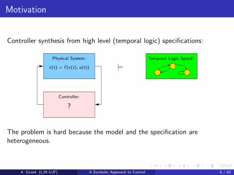
Controller synthesis from high level (temporal logic) specifications:
Temporal Logic Specif.:Physical System:
|=x(t) = f (x(t), u(t))
Controller:
?
The problem is hard because the model and the specification areheterogeneous.
A. Girard (LJK-UJF) A Symbolic Approach to Control 6 / 62

Symbolic Approach to Control Synthesis
Symbolic (discrete) model that is approximately equivalent to the(continuous) dynamics of the physical system:
Physical System:
≈x(t) = f (x(t), u(t))
Symbolic Model:
A. Girard (LJK-UJF) A Symbolic Approach to Control 7 / 62

Symbolic Approach to Control Synthesis
Symbolic (discrete) model that is approximately equivalent to the(continuous) dynamics of the physical system:
Discrete Controller:
Symbolic Model:Physical System:
x(t) = f (x(t), u(t))
A. Girard (LJK-UJF) A Symbolic Approach to Control 8 / 62
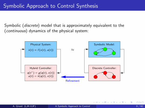
Symbolic Approach to Control Synthesis
Symbolic (discrete) model that is approximately equivalent to the(continuous) dynamics of the physical system:
Discrete Controller:
Symbolic Model:
Hybrid Controller:
Physical System:
≈x(t) = f (x(t), u(t))
Refinement
q(t+) = g(q(t), x(t))u(t) = k(q(t), x(t))
A. Girard (LJK-UJF) A Symbolic Approach to Control 9 / 62

Symbolic Approach to Control Synthesis
A three step approach to controller synthesis:1 Computation of a symbolic abstraction of the physical system.2 Discrete controller synthesis for the symbolic abstraction.3 Hybrid controller synthesis via discrete controller refinement.
This allows us to leverage discrete controller synthesis techniques:
Use supervisory control, algorithmic game theory...Modular approaches for rich specifications.Possibility of optimizing some performance criteria to choose amongadmissible controllers: dynamic programming, shortest path algorithms,branch and bound, α-β pruning...
A. Girard (LJK-UJF) A Symbolic Approach to Control 10 / 62

Outline of the Talk
1 Approximation relationships for discrete and continuous systems
Approximate bisimulation.Symbolic abstractions of switched systems.
2 Controller synthesis using approximately bisimilar abstractions
Synthesis for safety specifications.Synthesis for reachability specifications under time optimization.
A. Girard (LJK-UJF) A Symbolic Approach to Control 11 / 62

Transition Systems
Unified modeling framework of discrete and (sampled) continuous systems.
Definition
A transition system is a tuple T = (X ,U, δ,Y ,H) where
X is a (discrete or continuous) set of states;
U is a (discrete or continuous) set of inputs;
δ : X × U → 2X is a transition relation;
Y is a (discrete or continuous) set of outputs;
H : X → Y is an ouput map.
1
21
0
a, b
aa
a
a
b
bb
X = {red , blue, green, yellow}U = {a, b}Y = {0, 1, 2}
A. Girard (LJK-UJF) A Symbolic Approach to Control 12 / 62
Transition Systems
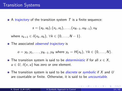
A trajectory of the transition system T is a finite sequence:
s = (x0, u0), (x1, u1), . . . , (xN−1, uN−1), xN
where xk+1 ∈ δ(xk , uk ), ∀k ∈ {0, . . . ,N − 1}.
The associated observed trajectory is
o = y0, y1, . . . , yN−1, yN where yk = H(xk ), ∀k ∈ {0, . . . ,N}.
The transition system is said to be deterministic if for all x ∈ X ,u ∈ U, δ(x , u) has zero or one element.
The transition system is said to be discrete or symbolic if X and Uare countable or finite. Otherwise, it is said to be uncountable.
A. Girard (LJK-UJF) A Symbolic Approach to Control 13 / 62

Approximate Bisimulation
Let Ti = (Xi ,U, δi ,Y ,Hi ), i ∈ {1, 2}, be transition systems with acommon set of inputs U and outputs O equipped with a metric d .
Definition
Let ε ∈ R+, a relation R ⊆ X1 × X2 is an ε-approximate bisimulationrelation if for all (x1, x2) ∈ R :
1 d(H1(x1),H2(x2)) ≤ ε;
2 ∀u ∈ U, ∀x ′1 ∈ δ1(x1, u), ∃x ′2 ∈ δ2(x2, u), such that (x ′1, x′2) ∈ R;
3 ∀u ∈ U, ∀x ′2 ∈ δ2(x2, u), ∃x ′1 ∈ δ1(x1, u), such that (x ′1, x′2) ∈ R.
Definition
T1 and T2 are ε-approximately bisimilar (T1 ∼ε T2) if :
1 For all x1 ∈ X1, there exists x2 ∈ X2, such that (x1, x2) ∈ R;
2 For all x2 ∈ X2, there exists x1 ∈ X1, such that (x1, x2) ∈ R.
A. Girard (LJK-UJF) A Symbolic Approach to Control 14 / 62

Approximate Bisimulation
X1
X2
d(H1(x1), H2(x2)) ≤ ε
R
x1
A. Girard (LJK-UJF) A Symbolic Approach to Control 15 / 62

Approximate Bisimulation
X1
X2
d(H1(x1), H2(x2)) ≤ ε
R
x1
x2
A. Girard (LJK-UJF) A Symbolic Approach to Control 16 / 62

Approximate Bisimulation
X1
X2
d(H1(x1), H2(x2)) ≤ ε
R
x1
x2
x′1 ∈ δ1(x1, u)
A. Girard (LJK-UJF) A Symbolic Approach to Control 17 / 62

Approximate Bisimulation
X1
X2
d(H1(x1), H2(x2)) ≤ ε
R
x1
x2
x′1 ∈ δ1(x1, u)
x′2 ∈ δ2(x2, u)
A. Girard (LJK-UJF) A Symbolic Approach to Control 18 / 62

Approximate Bisimulation
Proposition
If T1 ∼ε T2, then for all trajectories of T1, (x10 , u0), . . . , (x1
N−1, uN−1), x1N ,
there exists a trajectory of T2, (x20 , u0), . . . , (x2
N−1, uN−1), x2N with the
same sequence of inputs, such that
∀k ∈ {0, . . . ,N}, (x1k , x
2k ) ∈ R.
The associated observed trajectories y 10 , . . . , y
1N and y 2
0 , . . . , y2N satisfy
∀k ∈ {0, . . . ,N}, d(y 1k , y
2k ) ≤ ε.
For ε = 0, we recover the usual notion of bisimulation relation used incomputer science for studying equivalence of discrete systems.
A. Girard (LJK-UJF) A Symbolic Approach to Control 19 / 62

Outline of the Talk
1 Approximation relationships for discrete and continuous systems
Approximate bisimulation.Symbolic abstractions of switched systems.
2 Controller synthesis using approximately bisimilar abstractions
Synthesis for safety specifications.Synthesis for reachability specifications under time optimization.
A. Girard (LJK-UJF) A Symbolic Approach to Control 20 / 62

Switched Systems
Definition
A switched system is a tuple Σ = (Rn,P,F) where:
Rn is the state space;
P = {1, . . . ,m} is the finite set of modes;
F = {fp : Rn → Rn| p ∈ P} is the collection of vector fields.
For a switching signal p : R+ → P, initial state x ∈ Rn, x(t, x ,p)denotes the trajectory of Σ given by:
x(t) = fp(t)(x(t)), x(0) = x .
For p ∈ P, x(t, x , p) denotes the trajectory of Σ associated to theconstant switching signal p(t) = p.
A. Girard (LJK-UJF) A Symbolic Approach to Control 21 / 62

Switched Systems as Transition Systems
Consider a switched system Σ = (Rn,P,F) and a time samplingparameter τ > 0.
Let Tτ (Σ) be the transition system where:
the set of states is X = Rn;the set of inputs is U = P;the transition relation is given by
x ′ ∈ δ(x , p) ⇐⇒ x ′ = x(τ, x , p);
the set of outputs is Y = Rn;the output map H is the identity map over Rn.
The transition system Tτ (Σ) is uncountable, can we compute asymbolic abstraction?
A. Girard (LJK-UJF) A Symbolic Approach to Control 22 / 62

Computation of the Symbolic Abstraction
We start by approximating the set of states Rn by:
[Rn]η =
{z ∈ Rn
∣∣∣∣ zi = ki2η√
n, ki ∈ Z, i = 1, ..., n
},
where η > 0 is a state sampling parameter:
∀x ∈ Rn, ∃z ∈ [Rn]η, ‖x − z‖ ≤ η.
Approximation of the transition relation = “rounding”:
x(τ, z, p)
z
z ′
A. Girard (LJK-UJF) A Symbolic Approach to Control 23 / 62

Computation of the Symbolic Abstraction
We define the transition system Tτ,η(Σ) where :
the set of states is X = [Rn]η;the set of inputs is U = P;the transition relation is given by
z ′ ∈ δ(z , p) ⇐⇒ z ′ = arg minq∈[Rn]η
(‖x(τ, z , p)− q‖) .
the set of outputs is Y = Rn;the output map is given by H(z) = z ∈ Rn.
The transition system Tτ,η(Σ) is discrete and deterministic.
Are Tτ (Σ) and Tτ,η(Σ) approximately bisimilar ?
Yes, if switched system Σ is incrementally stable.
A. Girard (LJK-UJF) A Symbolic Approach to Control 24 / 62

Incremental Stability
Definition
The switched system Σ is incrementally globally uniformly asymptoticallystable (δ-GUAS) if there exists a KL function β such that for all initialconditions x1, x2 ∈ Rn, for all switching signals p : R+ → P, for all t ∈ R+:
‖x(t, x1,p)− x(t, x2,p)‖ ≤ β(‖x1 − x2‖, t)t→+∞
- 0.
t
x(t, x1, p)
x(t, x2, p)
A. Girard (LJK-UJF) A Symbolic Approach to Control 25 / 62

δ-GAS Lyapunov Functions
Definition
V : Rn ×Rn → R+ is a common δ-GUAS Lyapunov function for Σ if thereexist K∞ functions α, α and κ ∈ R+ such that for all x1, x2 ∈ Rn:
α(‖x1 − x2‖) ≤ V (x1, x2) ≤ α(‖x1 − x2‖),
∀p ∈ P,∂V
∂x1(x1, x2)fp(x1) +
∂V
∂x2(x1, x2)fp(x2) ≤ −κV (x1, x2).
Theorem
If there exists a common δ-GUAS Lyapunov function, then Σ is δ-GUAS.
Supplementary assumption (true if working on a compact subset of Rn):There exists a K∞ function γ such that
∀x1, x2, x3 ∈ Rn, |V (x1, x2)− V (x1, x3)| ≤ γ(‖x2 − x3‖).
A. Girard (LJK-UJF) A Symbolic Approach to Control 26 / 62

Approximation Theorem
Theorem
Let us assume that there exists V : Rn × Rn → R+ which is a commonδ-GUAS Lyapunov function for Σ. Consider sampling parametersτ, η ∈ R+ and a desired precision ε ∈ R+. If
η ≤ min{γ−1
((1− e−κτ )α(ε)
), α−1 (α(ε))
}
then, the relation R ⊆ Rn × [Rn]η given by
R = {(x , z) ∈ Rn × [Rn]η| V (x , z) ≤ α(ε)}
is an ε-approximate bisimulation relation and Tτ (Σ) ∼ε Tτ,η(Σ).
Main idea of the proof: show that accumulation of successive “roundingerrors” is contained by incremental stability.
A. Girard (LJK-UJF) A Symbolic Approach to Control 27 / 62

Comments on the Approximation Theorem
For a given time sampling parameter τ , any precision ε can beachieved by choosing appropriately the state sampling parameter η(the smaller τ or ε, the smaller η).
If all vector fields are affine, one can search for a quadratic commonδ-GUAS Lyapunov functions by solving a set of LMIs.
For switched systems that do not admit a common δ-GUAS Lyapunovfunctions, the result can be extended by using multiple δ-GUASLyapunov functions and by imposing a minimum dwell time.
A similar result applies to incrementally stable continuous controlsystems.
A. Girard (LJK-UJF) A Symbolic Approach to Control 28 / 62

Example: DC-DC Converter
Power converter with switching control:
il
s1
vs
rlxl
s2
xc
rc
vc
r0 v0
State variable: x(t) = [il (t), vc (t)]T .
System dynamics: x(t) = Apx(t) + b, p ∈ {1, 2}.
Common δ-GUAS Lyapunov function of the form:
V (x , y) =√
(x − y)T M(x − y).
A. Girard (LJK-UJF) A Symbolic Approach to Control 29 / 62

Example: Symbolic Abstraction of the DC-DC Converter
(Useless) symbolic abstraction: τ = 0.5, η = 140√
2=⇒ ε = 2.6.
A. Girard (LJK-UJF) A Symbolic Approach to Control 30 / 62

Outline of the Talk
1 Approximation relationships for discrete and continuous systems
Approximate bisimulation.Symbolic abstractions of switched systems.
2 Controller synthesis using approximately bisimilar abstractions
Synthesis for safety specifications.Synthesis for reachability specifications under time optimization.
A. Girard (LJK-UJF) A Symbolic Approach to Control 31 / 62
Controllers for Safety Specifications
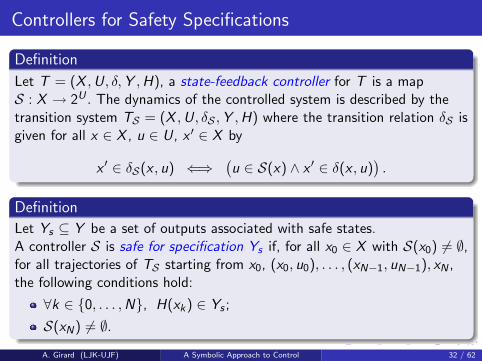
Definition
Let T = (X ,U, δ,Y ,H), a state-feedback controller for T is a mapS : X → 2U . The dynamics of the controlled system is described by thetransition system TS = (X ,U, δS ,Y ,H) where the transition relation δS isgiven for all x ∈ X , u ∈ U, x ′ ∈ X by
x ′ ∈ δS(x , u) ⇐⇒(u ∈ S(x) ∧ x ′ ∈ δ(x , u)
).
Definition
Let Ys ⊆ Y be a set of outputs associated with safe states.A controller S is safe for specification Ys if, for all x0 ∈ X with S(x0) 6= ∅,for all trajectories of TS starting from x0, (x0, u0), . . . , (xN−1, uN−1), xN ,the following conditions hold:
∀k ∈ {0, . . . ,N}, H(xk) ∈ Ys ;
S(xN) 6= ∅.
A. Girard (LJK-UJF) A Symbolic Approach to Control 32 / 62
Controllers for Safety Specifications
Definition
Let T = (X ,U, δ,Y ,H), a state-feedback controller for T is a mapS : X → 2U . The dynamics of the controlled system is described by thetransition system TS = (X ,U, δS ,Y ,H) where the transition relation δS isgiven for all x ∈ X , u ∈ U, x ′ ∈ X by
x ′ ∈ δS(x , u) ⇐⇒(u ∈ S(x) ∧ x ′ ∈ δ(x , u)
).
Definition
Let Ys ⊆ Y be a set of outputs associated with safe states.A controller S is safe for specification Ys if, for all x0 ∈ X with S(x0) 6= ∅,for all trajectories of TS starting from x0, (x0, u0), . . . , (xN−1, uN−1), xN ,the following conditions hold:
∀k ∈ {0, . . . ,N}, H(xk ) ∈ Ys ;
S(xN) 6= ∅.A. Girard (LJK-UJF) A Symbolic Approach to Control 32 / 62

Maximal Safe Controller
If for all x ∈ X , S(x) = ∅, then S is safe... We need a notion of “best”safe controller.
Definition
Controller S1 is more permissive than controller S2 (S2 � S1) if,for all x ∈ X , S2(x) ⊆ S1(x).
Definition
S∗ is the maximal safe controller for specification Ys if, S∗ is safe andfor all safe controllers S, S � S∗.
The maximal safe controller exists and is unique.
It can be determined by fixed point computation of the largestcontrolled-invariant of T , included in H−1(Ys).
A. Girard (LJK-UJF) A Symbolic Approach to Control 33 / 62

Computation of the Largest Controlled-Invariant
The controlled-predecessor of F ⊆ X is
Pred(F ) ={
x ∈ X | ∃u ∈ U, (δ(x , u) 6= ∅) ∧ (∀x ′ ∈ δ(x , u), x ′ ∈ F )}.
F is controlled-invariant if F ⊆ Pred(F ).
Algorithm
Computation of F ∗, largest controlled-invariant of T included in H−1(Ys):
F 0 := H−1(Ys)repeat∣∣ F k+1 := F k ∩ Pred(F k )until F k+1 = F k
F ∗ := F k
The algorithm terminates in a finite number of steps for discrete transitionsystems if H−1(Ys) is finite. No guarantee of termination for uncountabletransition systems.
A. Girard (LJK-UJF) A Symbolic Approach to Control 34 / 62

Computation of the Maximal Safe Controller
Theorem
Let S∗ : X → 2U be the controller for T defined, for all x ∈ X \ F ∗, byS∗(x) = ∅, and for all x ∈ F ∗ by
S∗(x) ={
u ∈ U| (δ(x , u) 6= ∅) ∧ (∀x ′ ∈ δ(x , u), x ′ ∈ F ∗)}.
Then, S∗ is the maximal safe controller for the specification Ys .
A simple example:a a
a
a
aa
a
a
b a
ba
bbb
A. Girard (LJK-UJF) A Symbolic Approach to Control 35 / 62
Computation of the Maximal Safe Controller
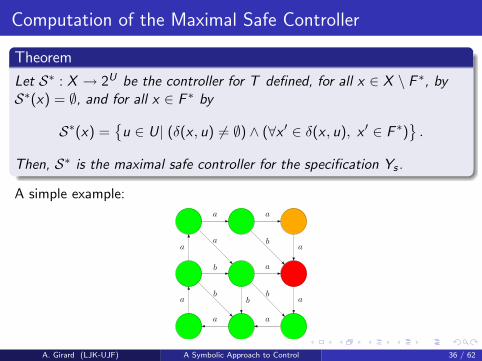
Theorem
Let S∗ : X → 2U be the controller for T defined, for all x ∈ X \ F ∗, byS∗(x) = ∅, and for all x ∈ F ∗ by
S∗(x) ={
u ∈ U| (δ(x , u) 6= ∅) ∧ (∀x ′ ∈ δ(x , u), x ′ ∈ F ∗)}.
Then, S∗ is the maximal safe controller for the specification Ys .
A simple example:a a
a
a
aa
a
a
b a
ba
bbb
A. Girard (LJK-UJF) A Symbolic Approach to Control 36 / 62

Computation of the Maximal Safe Controller
Theorem
Let S∗ : X → 2U be the controller for T defined, for all x ∈ X \ F ∗, byS∗(x) = ∅, and for all x ∈ F ∗ by
S∗(x) ={
u ∈ U| (δ(x , u) 6= ∅) ∧ (∀x ′ ∈ δ(x , u), x ′ ∈ F ∗)}.
Then, S∗ is the maximal safe controller for the specification Ys .
A simple example:a a
a
a
aa
a
a
b a
ba
bbb
A. Girard (LJK-UJF) A Symbolic Approach to Control 37 / 62

Computation of the Maximal Safe Controller
Theorem
Let S∗ : X → 2U be the controller for T defined, for all x ∈ X \ F ∗, byS∗(x) = ∅, and for all x ∈ F ∗ by
S∗(x) ={
u ∈ U| (δ(x , u) 6= ∅) ∧ (∀x ′ ∈ δ(x , u), x ′ ∈ F ∗)}.
Then, S∗ is the maximal safe controller for the specification Ys .
A simple example:a a
a
a
aa
a
a
b a
ba
bbb
A. Girard (LJK-UJF) A Symbolic Approach to Control 38 / 62

Computation of the Maximal Safe Controller
Theorem
Let S∗ : X → 2U be the controller for T defined, for all x ∈ X \ F ∗, byS∗(x) = ∅, and for all x ∈ F ∗ by
S∗(x) ={
u ∈ U| (δ(x , u) 6= ∅) ∧ (∀x ′ ∈ δ(x , u), x ′ ∈ F ∗)}.
Then, S∗ is the maximal safe controller for the specification Ys .
A simple example:a a
a
a
aa
a
a
b a
ba
bbb
A. Girard (LJK-UJF) A Symbolic Approach to Control 39 / 62
Safe Controller Synthesis via Symbolic Abstractions
Maximal safe controllers are easy to compute for symbolic abstractions...We need a controller refinement procedure!
Definition
Let Y ′ ⊆ Y and ϕ ≥ 0. The ϕ-contraction of Y ′ is the subset of Y isCϕ(Y ′) = {y ∈ Y ′| ∀y ′ ∈ Y , d(y , y ′) ≤ ϕ =⇒ y ′ ∈ Y ′} .
Theorem
Let T1 ∼ε T2, let R ⊆ X1 × X2 denote the ε-approximate bisimulationrelation between T1 and T2. Let S∗2,ε be the maximal safe controller forT2 for the specification Cε(Ys). Let S1 be the controller for T1 given by
∀x1 ∈ X1, S1(x1) =⋃
x2∈R(x1)
S∗2,ε(x2)
where x2 ∈ R(x1) means (x1, x2) ∈ R. Then, S1 is safe for specification Ys .
A. Girard (LJK-UJF) A Symbolic Approach to Control 40 / 62

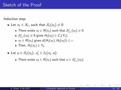
Sketch of the Proof
Induction step:
Let x1 ∈ X1, such that S1(x1) 6= ∅:
There exists x2 ∈ R(x1) such that S∗2,ε(x2) 6= ∅.S∗2,ε(x2) 6= ∅ gives H2(x2) ∈ Cε(Ys).
x2 ∈ R(x1) gives d(H1(x1),H2(x2)) ≤ ε.
Then, H1(x1) ∈ Ys .
Let u ∈ S1(x1), x ′1 ∈ δ1(x1, u):
There exists x2 ∈ R(x1) such that u ∈ S∗2,ε(x2).
x2 ∈ R(x1) gives that there exists x ′2 ∈ δ2(x2, u) such that x ′2 ∈ R(x ′1).
u ∈ S∗2,ε(x2) gives S∗2,ε(x ′2) 6= ∅.Then, S1(x ′1) 6= ∅.
A. Girard (LJK-UJF) A Symbolic Approach to Control 41 / 62

Sketch of the Proof
Induction step:
Let x1 ∈ X1, such that S1(x1) 6= ∅:There exists x2 ∈ R(x1) such that S∗2,ε(x2) 6= ∅.
S∗2,ε(x2) 6= ∅ gives H2(x2) ∈ Cε(Ys).
x2 ∈ R(x1) gives d(H1(x1),H2(x2)) ≤ ε.
Then, H1(x1) ∈ Ys .
Let u ∈ S1(x1), x ′1 ∈ δ1(x1, u):
There exists x2 ∈ R(x1) such that u ∈ S∗2,ε(x2).
x2 ∈ R(x1) gives that there exists x ′2 ∈ δ2(x2, u) such that x ′2 ∈ R(x ′1).
u ∈ S∗2,ε(x2) gives S∗2,ε(x ′2) 6= ∅.Then, S1(x ′1) 6= ∅.
A. Girard (LJK-UJF) A Symbolic Approach to Control 41 / 62

Sketch of the Proof
Induction step:
Let x1 ∈ X1, such that S1(x1) 6= ∅:There exists x2 ∈ R(x1) such that S∗2,ε(x2) 6= ∅.S∗2,ε(x2) 6= ∅ gives H2(x2) ∈ Cε(Ys).
x2 ∈ R(x1) gives d(H1(x1),H2(x2)) ≤ ε.
Then, H1(x1) ∈ Ys .
Let u ∈ S1(x1), x ′1 ∈ δ1(x1, u):
There exists x2 ∈ R(x1) such that u ∈ S∗2,ε(x2).
x2 ∈ R(x1) gives that there exists x ′2 ∈ δ2(x2, u) such that x ′2 ∈ R(x ′1).
u ∈ S∗2,ε(x2) gives S∗2,ε(x ′2) 6= ∅.Then, S1(x ′1) 6= ∅.
A. Girard (LJK-UJF) A Symbolic Approach to Control 41 / 62

Sketch of the Proof
Induction step:
Let x1 ∈ X1, such that S1(x1) 6= ∅:There exists x2 ∈ R(x1) such that S∗2,ε(x2) 6= ∅.S∗2,ε(x2) 6= ∅ gives H2(x2) ∈ Cε(Ys).
x2 ∈ R(x1) gives d(H1(x1),H2(x2)) ≤ ε.
Then, H1(x1) ∈ Ys .
Let u ∈ S1(x1), x ′1 ∈ δ1(x1, u):
There exists x2 ∈ R(x1) such that u ∈ S∗2,ε(x2).
x2 ∈ R(x1) gives that there exists x ′2 ∈ δ2(x2, u) such that x ′2 ∈ R(x ′1).
u ∈ S∗2,ε(x2) gives S∗2,ε(x ′2) 6= ∅.
Then, S1(x ′1) 6= ∅.
A. Girard (LJK-UJF) A Symbolic Approach to Control 41 / 62

Sketch of the Proof
Induction step:
Let x1 ∈ X1, such that S1(x1) 6= ∅:There exists x2 ∈ R(x1) such that S∗2,ε(x2) 6= ∅.S∗2,ε(x2) 6= ∅ gives H2(x2) ∈ Cε(Ys).
x2 ∈ R(x1) gives d(H1(x1),H2(x2)) ≤ ε.
Then, H1(x1) ∈ Ys .
Let u ∈ S1(x1), x ′1 ∈ δ1(x1, u):
There exists x2 ∈ R(x1) such that u ∈ S∗2,ε(x2).
x2 ∈ R(x1) gives that there exists x ′2 ∈ δ2(x2, u) such that x ′2 ∈ R(x ′1).
u ∈ S∗2,ε(x2) gives S∗2,ε(x ′2) 6= ∅.Then, S1(x ′1) 6= ∅.
A. Girard (LJK-UJF) A Symbolic Approach to Control 41 / 62

Distance to the Maximal Safe Controller
Theorem
Let S1 be the safe controller for T1 for specification Ys defined in theprevious theorem. Let S∗1 and S∗1,2ε be the maximal safe controllers for T1
for specifications Ys and C2ε(Ys), respectively. Then,
S∗1,2ε � S1 � S∗1 .
Sketch of proof:
S∗1,2ε(q1) S∗1(q1)S1(q1) =⋃
q2∈R(q1)S∗2,ε(q2)
S∗2,ε(q2)
⊆
ref
A. Girard (LJK-UJF) A Symbolic Approach to Control 42 / 62

Distance to the Maximal Safe Controller
Theorem
Let S1 be the safe controller for T1 for specification Ys defined in theprevious theorem. Let S∗1 and S∗1,2ε be the maximal safe controllers for T1
for specifications Ys and C2ε(Ys), respectively. Then,
S∗1,2ε � S1 � S∗1 .
Sketch of proof:
S∗1,2ε(q1) S∗1(q1)S1(q1) =⋃
q2∈R(q1)S∗2,ε(q2)
⊆S2,ε(q2) =⋃
q1∈R−1(q2)S∗1,2ε(q1) S∗2,ε(q2)
⊆
ref ref
A. Girard (LJK-UJF) A Symbolic Approach to Control 43 / 62

Distance to the Maximal Safe Controller
Theorem
Let S1 be the safe controller for T1 for specification Ys defined in theprevious theorem. Let S∗1 and S∗1,2ε be the maximal safe controllers for T1
for specifications Ys and C2ε(Ys), respectively. Then,
S∗1,2ε � S1 � S∗1 .
Sketch of proof:
S∗1,2ε(q1) S∗1(q1)S1(q1) =⋃
q2∈R(q1)S∗2,ε(q2)
⊆S2,ε(q2) =⋃
q1∈R−1(q2)S∗1,2ε(q1)
S1(q1) =⋃
q2∈R(q1)S2,ε(q2)
S∗2,ε(q2)
⊆⊆⊆
ref ref ref
A. Girard (LJK-UJF) A Symbolic Approach to Control 44 / 62

Example: Safe Controller for the DC-DC Converter
Abstraction parameters: τ = 0.5, η = 17× 10−5 =⇒ ε = 25× 10−3.
Ys = [1.275, 1.525]× [5.625, 5.775] =⇒ Cε(Ys) = [1.3, 1.5]× [5.65, 5.75].
The symbolic abstraction has 337431 states, the synthesis algorithmterminates in 5 iterations.
1.3 1.32 1.34 1.36 1.38 1.4 1.42 1.44 1.46 1.485.65
5.66
5.67
5.68
5.69
5.7
5.71
5.72
5.73
5.74
5.75
1.3 1.35 1.4 1.45 1.5
5.64
5.66
5.68
5.7
5.72
5.74
5.76
S∗2,ε S1
A. Girard (LJK-UJF) A Symbolic Approach to Control 45 / 62

Example: Safe Controller for the DC-DC Converter
The synthesized controller is non-deterministic.
Several implementations of the controller are possible.
Possibility to ensure a posteriori secondary control objective.
1.3 1.35 1.4 1.45 1.5
5.64
5.66
5.68
5.7
5.72
5.74
5.76
1.3 1.35 1.4 1.45 1.5
5.64
5.66
5.68
5.7
5.72
5.74
5.76
Lazy control Stochastic control
A. Girard (LJK-UJF) A Symbolic Approach to Control 46 / 62

Outline of the Talk
1 Approximation relationships for discrete and continuous systems
Approximate bisimulation.Symbolic abstractions of switched systems.
2 Controller synthesis using approximately bisimilar abstractions
Synthesis for safety specifications.Synthesis for reachability specifications under time optimization.
A. Girard (LJK-UJF) A Symbolic Approach to Control 47 / 62

Controllers for Reachability Specifications
The goal is to steer the state of the system to a desired target whilekeeping the system safe along the way.
Definition
Let T = (X ,U, δ,Y ,H) and S : X → 2U be a controller for T .Let Ys ⊆ Y be a set of outputs associated with safe states andYt ⊆ Ys be a set of outputs associated with target states.The entry time of TS from x0 ∈ X for specification (Ys ,Yt) is the smallestN ∈ N such that for all trajectories of TS of length N and starting fromx0, (x0, u0), . . . , (xN−1, uN−1), xN , there exists K ∈ {0, . . . ,N} such that:
∀k ∈ {0, . . . ,K}, H(xk ) ∈ Ys ;
H(xK ) ∈ Yt .
The entry time is denoted by J(TS ,Ys ,Yt , x0).If such N does not exist, then we define J(TS ,Ys ,Yt , x0) = +∞.
A. Girard (LJK-UJF) A Symbolic Approach to Control 48 / 62

Time-Optimal Controller
The control objective is to minimize the entry time.
Definition
We say that a controller S∗ is time-optimal for specification (Ys ,Yt) if,for all controllers S:
∀x ∈ X , J(TS∗ ,Ys ,Yt , x) ≤ J(TS ,Ys ,Yt , x).
We define the value function of the time-optimal control problem asJ∗(T ,Ys ,Yt , x) = J(TS∗ ,Ys ,Yt , x).
There exists a time-optimal controller (may be not unique).
It can be determined by dynamic programming and fixed pointcomputation of the value function of the time-optimal controlproblem.
A. Girard (LJK-UJF) A Symbolic Approach to Control 49 / 62
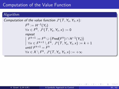
Computation of the Value Function
Algorithm
Computation of the value function J∗(T ,Ys ,Yt , x):
F 0 := H−1(Yt)∀x ∈ F 0, J∗(T ,Ys ,Yt , x) := 0repeat∣∣∣∣
F k+1 := F k ∪(Pred(F k ) ∩ H−1(Ys)
)
∀x ∈ F k+1 \ F k , J∗(T ,Ys ,Yt , x) := k + 1until F k+1 = F k
∀x ∈ X \ F k , J∗(T ,Ys ,Yt , x) := +∞
F k is the set of states from which the system can reach the target inat most k transitions while remaining in the safe set.
The algorithm terminates in a finite number of steps for discretetransition systems if H−1(Ys) is finite. No guarantee of terminationfor infinite transition systems.
A. Girard (LJK-UJF) A Symbolic Approach to Control 50 / 62

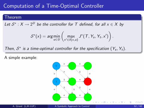
Computation of a Time-Optimal Controller
Theorem
Let S∗ : X → 2U be the controller for T defined, for all x ∈ X by
S∗(x) = arg minu∈U
(max
x ′∈δ(x ,u)J∗(T ,Ys ,Yt , x
′)
).
Then, S∗ is a time-optimal controller for the specification (Ys ,Yt).
A simple example:
a a
a
a
aa
a
a
b a
ba
bbb
0
A. Girard (LJK-UJF) A Symbolic Approach to Control 51 / 62
Computation of a Time-Optimal Controller
Theorem
Let S∗ : X → 2U be the controller for T defined, for all x ∈ X by
S∗(x) = arg minu∈U
(max
x ′∈δ(x ,u)J∗(T ,Ys ,Yt , x
′)
).
Then, S∗ is a time-optimal controller for the specification (Ys ,Yt).
A simple example:
a a
a
a
aa
a
a
b a
ba
bbb
0
1
A. Girard (LJK-UJF) A Symbolic Approach to Control 52 / 62

Computation of a Time-Optimal Controller
Theorem
Let S∗ : X → 2U be the controller for T defined, for all x ∈ X by
S∗(x) = arg minu∈U
(max
x ′∈δ(x ,u)J∗(T ,Ys ,Yt , x
′)
).
Then, S∗ is a time-optimal controller for the specification (Ys ,Yt).
A simple example:
a a
a
a
aa
a
a
b a
ba
bbb
0
1
2
A. Girard (LJK-UJF) A Symbolic Approach to Control 53 / 62

Computation of a Time-Optimal Controller
Theorem
Let S∗ : X → 2U be the controller for T defined, for all x ∈ X by
S∗(x) = arg minu∈U
(max
x ′∈δ(x ,u)J∗(T ,Ys ,Yt , x
′)
).
Then, S∗ is a time-optimal controller for the specification (Ys ,Yt).
A simple example:
a a
a
a
aa
a
a
b a
ba
bbb
0
1
2 3
A. Girard (LJK-UJF) A Symbolic Approach to Control 54 / 62

Computation of a Time-Optimal Controller
Theorem
Let S∗ : X → 2U be the controller for T defined, for all x ∈ X by
S∗(x) = arg minu∈U
(max
x ′∈δ(x ,u)J∗(T ,Ys ,Yt , x
′)
).
Then, S∗ is a time-optimal controller for the specification (Ys ,Yt).
A simple example:
a a
a
a
aa
a
a
b a
ba
bbb
0
1
2 3 4
A. Girard (LJK-UJF) A Symbolic Approach to Control 55 / 62

Computation of a Time-Optimal Controller
Theorem
Let S∗ : X → 2U be the controller for T defined, for all x ∈ X by
S∗(x) = arg minu∈U
(max
x ′∈δ(x ,u)J∗(T ,Ys ,Yt , x
′)
).
Then, S∗ is a time-optimal controller for the specification (Ys ,Yt).
A simple example:
a a
a
a
aa
a
a
b a
ba
bbb
0
1
2 3 4
5 +∞
+∞+∞
A. Girard (LJK-UJF) A Symbolic Approach to Control 56 / 62

Computation of a Time-Optimal Controller
Theorem
Let S∗ : X → 2U be the controller for T defined, for all x ∈ X by
S∗(x) = arg minu∈U
(max
x ′∈δ(x ,u)J∗(T ,Ys ,Yt , x
′)
).
Then, S∗ is a time-optimal controller for the specification (Ys ,Yt).
A simple example:
a a
a
a
aa
a
a
b a
ba
bbb
0
1
2 3 4
5 +∞
+∞+∞
A. Girard (LJK-UJF) A Symbolic Approach to Control 57 / 62

Suboptimal Controller Synthesis via Symbolic Abstractions
Time-optimal controllers are easy to compute for symbolic abstractions...We need a controller refinement procedure!
Theorem
Let T1 ∼ε T2, let R ⊆ X1 × X2 denote the ε-approximate bisimulationrelation between T1 and T2. Let S∗2,ε be a time-optimal controller for T2
for the specification (Cε(Ys),Cε(Yt)). Let S1 be the controller for T1
given by
∀x1 ∈ X1, S1(x1) = S∗2,ε(
arg minx2∈R(x1)
J∗(T2,Cε(Ys),Cε(Yt), x2)
).
The entry time of TS1 for specification (Ys ,Yt) satisfies for all x1 ∈ X1:
J∗(T1,Ys ,Yt , x1) ≤ J(T1,S1 ,Ys ,Yt , x1) ≤ J∗(T1,C2ε(Ys),C2ε(Yt), x1).
Proof is close to the case of safety controllers.
A. Girard (LJK-UJF) A Symbolic Approach to Control 58 / 62
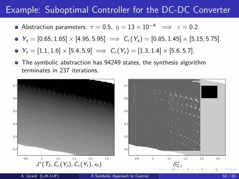
Example: Suboptimal Controller for the DC-DC Converter
Abstraction parameters: τ = 0.5, η = 13× 10−4 =⇒ ε = 0.2.
Ys = [0.65, 1.65]× [4.95, 5.95] =⇒ Cε(Ys) = [0.85, 1.45]× [5.15, 5.75].
Yt = [1.1, 1.6]× [5.4, 5.9] =⇒ Cε(Yt) = [1.3, 1.4]× [5.6, 5.7].
The symbolic abstraction has 94249 states, the synthesis algorithmterminates in 237 iterations.
0.9 1 1.1 1.2 1.3 1.4
5.2
5.3
5.4
5.5
5.6
5.7
0.9 1 1.1 1.2 1.3 1.4
5.2
5.3
5.4
5.5
5.6
5.7
J∗(T2, Cε(Ys ), Cε(Yt), x2) S∗2,ε
A. Girard (LJK-UJF) A Symbolic Approach to Control 59 / 62

Example: Suboptimal Controller for the DC-DC Converter
Suboptimal controller computed using the refinement procedure.
Controller S1 seems to be more “regular” than S2,ε.
Entry time ranges from 0 to 94 when J∗(T2,Cε(Ys),Cε(Yt), x2)ranges from 0 to 237.
0.7 0.8 0.9 1 1.1 1.2 1.3 1.4 1.5 1.6
5
5.1
5.2
5.3
5.4
5.5
5.6
5.7
5.8
5.9
0.7 0.8 0.9 1 1.1 1.2 1.3 1.4 1.5 1.6
5
5.1
5.2
5.3
5.4
5.5
5.6
5.7
5.8
5.9
J(T1,S1 , Ys , Yt , x1) S1
A. Girard (LJK-UJF) A Symbolic Approach to Control 60 / 62

Conclusions
Approximately bisimilar symbolic abstractions:
A rigorous tool for controller synthesis: controllers are “correct bydesign” with bounds on the distance to optimality...Allows to leverage efficient algorithmic techniques from discretesystems to continuous and hybrid systems.Computable for interesting classes of systems: switched systems,continuous control systems...Incremental stability needed for approximate bisimulation.
Ongoing and future work:
Multiscale and adaptive symbolic models.On the fly computation of symbolic models.Controller synthesis for other type of specifications.Complexity reduction of synthesized controllers.
A. Girard (LJK-UJF) A Symbolic Approach to Control 61 / 62

Conclusions
Approximately bisimilar symbolic abstractions:
A rigorous tool for controller synthesis: controllers are “correct bydesign” with bounds on the distance to optimality...
Allows to leverage efficient algorithmic techniques from discretesystems to continuous and hybrid systems.Computable for interesting classes of systems: switched systems,continuous control systems...Incremental stability needed for approximate bisimulation.
Ongoing and future work:
Multiscale and adaptive symbolic models.On the fly computation of symbolic models.Controller synthesis for other type of specifications.Complexity reduction of synthesized controllers.
A. Girard (LJK-UJF) A Symbolic Approach to Control 61 / 62
Conclusions
Approximately bisimilar symbolic abstractions:
A rigorous tool for controller synthesis: controllers are “correct bydesign” with bounds on the distance to optimality...Allows to leverage efficient algorithmic techniques from discretesystems to continuous and hybrid systems.
Computable for interesting classes of systems: switched systems,continuous control systems...Incremental stability needed for approximate bisimulation.
Ongoing and future work:
Multiscale and adaptive symbolic models.On the fly computation of symbolic models.Controller synthesis for other type of specifications.Complexity reduction of synthesized controllers.
A. Girard (LJK-UJF) A Symbolic Approach to Control 61 / 62

Conclusions
Approximately bisimilar symbolic abstractions:
A rigorous tool for controller synthesis: controllers are “correct bydesign” with bounds on the distance to optimality...Allows to leverage efficient algorithmic techniques from discretesystems to continuous and hybrid systems.Computable for interesting classes of systems: switched systems,continuous control systems...
Incremental stability needed for approximate bisimulation.
Ongoing and future work:
Multiscale and adaptive symbolic models.On the fly computation of symbolic models.Controller synthesis for other type of specifications.Complexity reduction of synthesized controllers.
A. Girard (LJK-UJF) A Symbolic Approach to Control 61 / 62

Conclusions
Approximately bisimilar symbolic abstractions:
A rigorous tool for controller synthesis: controllers are “correct bydesign” with bounds on the distance to optimality...Allows to leverage efficient algorithmic techniques from discretesystems to continuous and hybrid systems.Computable for interesting classes of systems: switched systems,continuous control systems...Incremental stability needed for approximate bisimulation.
Ongoing and future work:
Multiscale and adaptive symbolic models.On the fly computation of symbolic models.Controller synthesis for other type of specifications.Complexity reduction of synthesized controllers.
A. Girard (LJK-UJF) A Symbolic Approach to Control 61 / 62

Conclusions
Approximately bisimilar symbolic abstractions:
A rigorous tool for controller synthesis: controllers are “correct bydesign” with bounds on the distance to optimality...Allows to leverage efficient algorithmic techniques from discretesystems to continuous and hybrid systems.Computable for interesting classes of systems: switched systems,continuous control systems...Incremental stability needed for approximate bisimulation.
Ongoing and future work:
Multiscale and adaptive symbolic models.
On the fly computation of symbolic models.Controller synthesis for other type of specifications.Complexity reduction of synthesized controllers.
A. Girard (LJK-UJF) A Symbolic Approach to Control 61 / 62

Conclusions
Approximately bisimilar symbolic abstractions:
A rigorous tool for controller synthesis: controllers are “correct bydesign” with bounds on the distance to optimality...Allows to leverage efficient algorithmic techniques from discretesystems to continuous and hybrid systems.Computable for interesting classes of systems: switched systems,continuous control systems...Incremental stability needed for approximate bisimulation.
Ongoing and future work:
Multiscale and adaptive symbolic models.On the fly computation of symbolic models.
Controller synthesis for other type of specifications.Complexity reduction of synthesized controllers.
A. Girard (LJK-UJF) A Symbolic Approach to Control 61 / 62

Conclusions
Approximately bisimilar symbolic abstractions:
A rigorous tool for controller synthesis: controllers are “correct bydesign” with bounds on the distance to optimality...Allows to leverage efficient algorithmic techniques from discretesystems to continuous and hybrid systems.Computable for interesting classes of systems: switched systems,continuous control systems...Incremental stability needed for approximate bisimulation.
Ongoing and future work:
Multiscale and adaptive symbolic models.On the fly computation of symbolic models.Controller synthesis for other type of specifications.
Complexity reduction of synthesized controllers.
A. Girard (LJK-UJF) A Symbolic Approach to Control 61 / 62

Conclusions
Approximately bisimilar symbolic abstractions:
A rigorous tool for controller synthesis: controllers are “correct bydesign” with bounds on the distance to optimality...Allows to leverage efficient algorithmic techniques from discretesystems to continuous and hybrid systems.Computable for interesting classes of systems: switched systems,continuous control systems...Incremental stability needed for approximate bisimulation.
Ongoing and future work:
Multiscale and adaptive symbolic models.On the fly computation of symbolic models.Controller synthesis for other type of specifications.Complexity reduction of synthesized controllers.
A. Girard (LJK-UJF) A Symbolic Approach to Control 61 / 62

References
Approximation relationships for systems:Girard and Pappas, Approximation metrics for discrete and continuoussystems. IEEE TAC, 52(5):782-798, 2007.
Computation of approximately bisimilar abstractions:
Girard, Pola and Tabuada, Approximately bisimilar symbolic models for
incrementally stable switched systems. IEEE TAC, 55(1):116-126, 2010.
Pola, Girard and Tabuada, Approximately bisimilar symbolic models for
nonlinear control systems. Automatica, 44(10):2508-2516, 2008.Girard, Approximately bisimilar finite abstractions of stable linear systems.HSCC, vol 4416 in LNCS, pp 231-244, Springer, 2007.
Synthesis using approximately bisimilar abstractions:
Girard, Synthesis using approximately bisimilar abstractions: state-feedback
controllers for safety specifications. HSCC, 2010, to appear.
Girard, Synthesis using approximately bisimilar abstractions: time-optimal
control problems. 2010, submitted.
A. Girard (LJK-UJF) A Symbolic Approach to Control 62 / 62