a template tutorial - home | university of colorado · pdf filea template tutorial carlos a....
TRANSCRIPT

.
COMPUTATIONAL MECHANICS - THEORY AND PRACTICE
K.M. Mathisen, T. Kvamsdal and K.M. Okstad (Eds.)
c© CIMNE, Barcelona, Spain 2003
A TEMPLATE TUTORIAL
Carlos A. Felippa
Department of Aerospace Engineering Sciencesand Center for Aerospace StructuresUniversity of Colorado, CB 429Boulder, CO 80309-0429, USAEmail: [email protected] page: http://titan.colorado.edu/Felippa.d/FelippaHome.d/Home.html
Dedicated to Pal Bergan on his 60th birthday
Abstract. This article has a dual theme: historical and educational. It is a tutorial on finiteelement templates for two-dimensional structural problems. The exposition is aimed atreaders with introductory level knowledge of finite element methods. It focuses on thefour-node plane stress element of flat rectangular geometry, called the “rectangular panel”for brevity. This is one of the two oldest continuum structural elements. On the other handthe concept of finite element templates is a recent development, which had as key sourcethe 1984–87 collaboration between Pal Bergan and the writer on the Free Formulation.Interweaving the old and the new throws historical perspective into the evolution of finiteelement methods. Templates provide a framework in which diverse element formulationscan be fitted, compared and traced back to the sources. On the technical side templatesfacilitate the unified implementation of element families, as well as the construction ofcustom elements. To illustrate customization power beyond the rectangle, the Appendixpresents the construction of a four-noded bending-optimal trapezoid. This model sidestepsMacNeal’s limitation theorem in that it passes the patch test for any geometry while stayingbending-optimal along one direction and retaining full rank.
Key words: finite elements, history, templates, families, clones, quadrilateral membrane,Free Formulation, patch test
1 INTRODUCTION
This article interweaves historical and educational themes with the presentation of anew methodology for finite element development. It is expository in nature, and focuseson “FEM by its history.” It gently exposes the reader to the concept of templates, andexplains why they emerge naturally from historical evolution. Much of the material istutorial in nature, with some extracted from a FEM course offered by the writer.
Templates are parametrized algebraic forms that provide a continuum of consistent andstable finite element models of a given type and node/freedom configuration. Templateinstances produced by setting values to free parameters furnish specific elements. Ifthe template embodies all possible consistent and stable elements of a given type andconfiguration, it is called universal.
1

CARLOS A. FELIPPA / A Template Tutorial
Befitting the tutorial aim, the main body of this article focuses on the simplest two-dimensional element that possesses a nontrivial template: the four-node plane stress ele-ment of flat rectangular geometry. [The three-node linear triangle is simpler but its templateis trivial.] This is called the rectangular panel for brevity.
The rectangular panel is interesting from both historical and instructional viewpointsbecause:1. It is one of the two oldest continuum finite elements, the other being the linear
triangle.1
2. Along with its plane strain and axisymmetric cousins, it is the configuration treatedby most new methods since the birth of finite elements. As such it represents anin-vivo specimen of FEM evolution over the past 50 years.
3. It is amenable to complete analytical development, even for anisotropic materialbehavior. This makes the element particularly suitable for homework and projectassignments.
4. Analytical forms make the concept of signatures and clones highly visible to students.The paper is organized as follows. Section 2 is a brief outline of element formulation
approaches used from 1950 to date. Section 3 introduces the focus problem. Sections4–6 follow up on the historical theme by presenting stress, strain and displacement-basedmodels for the rectangular panel.
The concept of template is introduced in Section 7 by calling attention to a commonstructure that lurks behind the stiffness expressions of stress, strain and displacementmodels. Template terminology follows as consequence: families, signatures, instancesand clones. The role of higher order patch tests in optimality is illustrated in Sections 8and 9. SRI schemes are presented in Section 10 from the template standpoint to showthat this approach naturally leads to correct splittings of the elasticity law. The concept ofelement families is illustrated in Section 11 using stress hybrid and displacement bubbles asexamples. These clearly illuminate the futility of the “enrichment” approaches popular inthe late sixties. Section 12 provides numerical examples and Section 13 offers conclusions.
The Appendix presents the construction of a four-noded bending-optimal trapezoid.Although this illustrates the customization power of templates beyond rectangles, themore advanced mathematical tools in use behind the scenes can make the results look likeblack magic to beginners. The optimal trapezoid partly circumvents MacNeal’s limitationtheorem2 in that it passes the patch test for arbitrary geometry and material and is bendingoptimal along one direction, while retaining a bounded condition number and thus fulfillingthe inf-sup condition.
A sequel to this article3 covers the generalization to an a optimal quadrilateral ofarbitrary shape. The algebraic manipulations are beyond the power of any human to workout by hand over a lifetime, so in retrospect it is not surprising that this model has notbeen discovered sooner. Fortunately the symbolic work falls, although barely, within thegrasp of computer algebra systems on a PC. The final results are surprisingly simple andelegant, even for arbitrary anisotropic material. The construction finishes a quest that haspreoccupied FEM investigators over several decades.
2 HISTORICAL SKETCH
This section summarizes the history of structural finite elements since 1950 to date. Itfunctions as a hub for dispersed historical references. Readers uninterested in these aspectsshould proceed directly to Section 3. For exposition convenience, structural “finitelemen-tology” may be divided into four generations that span 10 to 15 years each. There are nosharp intergenerational breaks, but noticeable changes of emphasis. The ensuing outline
2
COMPUTATIONAL MECHANICS – THEORY AND PRACTICE
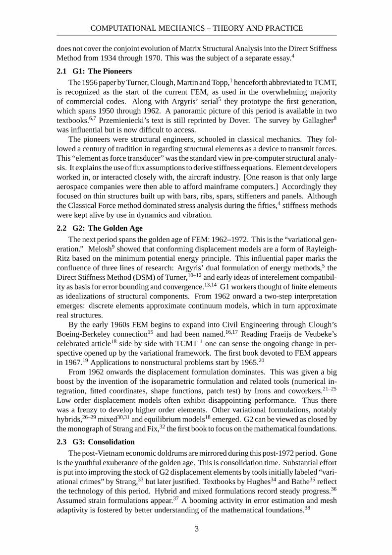
does not cover the conjoint evolution of Matrix Structural Analysis into the Direct StiffnessMethod from 1934 through 1970. This was the subject of a separate essay.4
2.1 G1: The PioneersThe 1956 paper by Turner, Clough, Martin and Topp,1 henceforth abbreviated to TCMT,
is recognized as the start of the current FEM, as used in the overwhelming majorityof commercial codes. Along with Argyris’ serial5 they prototype the first generation,which spans 1950 through 1962. A panoramic picture of this period is available in twotextbooks.6,7 Przemieniecki’s text is still reprinted by Dover. The survey by Gallagher8
was influential but is now difficult to access.The pioneers were structural engineers, schooled in classical mechanics. They fol-
lowed a century of tradition in regarding structural elements as a device to transmit forces.This “element as force transducer” was the standard view in pre-computer structural analy-sis. It explains the use of flux assumptions to derive stiffness equations. Element developersworked in, or interacted closely with, the aircraft industry. [One reason is that only largeaerospace companies were then able to afford mainframe computers.] Accordingly theyfocused on thin structures built up with bars, ribs, spars, stiffeners and panels. Althoughthe Classical Force method dominated stress analysis during the fifties,4 stiffness methodswere kept alive by use in dynamics and vibration.
2.2 G2: The Golden AgeThe next period spans the golden age of FEM: 1962–1972. This is the “variational gen-
eration.” Melosh9 showed that conforming displacement models are a form of Rayleigh-Ritz based on the minimum potential energy principle. This influential paper marks theconfluence of three lines of research: Argyris’ dual formulation of energy methods,5 theDirect Stiffness Method (DSM) of Turner,10–12 and early ideas of interelement compatibil-ity as basis for error bounding and convergence.13,14 G1 workers thought of finite elementsas idealizations of structural components. From 1962 onward a two-step interpretationemerges: discrete elements approximate continuum models, which in turn approximatereal structures.
By the early 1960s FEM begins to expand into Civil Engineering through Clough’sBoeing-Berkeley connection15 and had been named.16,17 Reading Fraeijs de Veubeke’scelebrated article18 side by side with TCMT 1 one can sense the ongoing change in per-spective opened up by the variational framework. The first book devoted to FEM appearsin 1967.19 Applications to nonstructural problems start by 1965.20
From 1962 onwards the displacement formulation dominates. This was given a bigboost by the invention of the isoparametric formulation and related tools (numerical in-tegration, fitted coordinates, shape functions, patch test) by Irons and coworkers.21–25
Low order displacement models often exhibit disappointing performance. Thus therewas a frenzy to develop higher order elements. Other variational formulations, notablyhybrids,26–29 mixed30,31 and equilibrium models18 emerged. G2 can be viewed as closed bythe monograph of Strang and Fix,32 the first book to focus on the mathematical foundations.
2.3 G3: ConsolidationThe post-Vietnam economic doldrums are mirrored during this post-1972 period. Gone
is the youthful exuberance of the golden age. This is consolidation time. Substantial effortis put into improving the stock of G2 displacement elements by tools initially labeled “vari-ational crimes” by Strang,33 but later justified. Textbooks by Hughes34 and Bathe35 reflectthe technology of this period. Hybrid and mixed formulations record steady progress.36
Assumed strain formulations appear.37 A booming activity in error estimation and meshadaptivity is fostered by better understanding of the mathematical foundations.38
3
CARLOS A. FELIPPA / A Template Tutorial
Commercial FEM codes gradually gain importance. They provide a reality check onwhat works in the real world and what doesn’t. By the mid-1980s there was gatheringevidence that complex and high order elements were commercial flops. Exotic gadgetryinterweaved amidst millions of lines of code easily breaks down in new releases. Com-plexity is particularly dangerous in nonlinear and dynamic analyses conducted by noviceusers. A trend back toward simplicity starts.39,40
2.4 G4: Back to Basics
The fourth generation begins by the early 1980s. More approaches come on the scene,notably the Free Formulation of Bergan,41,42 which is further discussed below, orthogonalhourglass control,43 Assumed Natural Strain methods,44–47 stress hybrid models in naturalcoordinates,48–50 as well as variants and derivatives of those approaches: ANDES,51,52
EAS53,54 and others. Although technically diverse the G4 approaches share two commonobjectives:(i) Elements must fit into DSM-based programs since that includes the vast majority of
production codes, commercial or otherwise.(ii) Elements are kept simple but should provide answers of engineering accuracy with
relatively coarse meshes. These were collectively labeled “high performance ele-ments” in 1989.55
“Things are always at their best in the beginning,” said Pascal. Indeed. By now FEMlooks like an aggregate of largely disconnected methods and recipes. Sections 4-6 lookat three disparate components of this edifice to anticipate the subsequent exhibition ofcommon features by templates.
2.5 From the Free Formulation to Templates
In the early 1970s Pal Bergan — then a Professor at NTH-Trondheim — and L. Hanssenpublished a paper56 in MAFELAP II, where a different approach to finite elements wasadvocated. The concept is well outlined in the Introduction of that paper:
“An important observation is that each element is, in fact, only represented by the numbers in itsstiffness matrix during the analysis of the assembled system. The origin of these stiffness coefficientsis unimportant to this part of the solution process ... The present approach is in a sense the opposite ofthat normally used in that the starting point is a generally formulated convergence condition and fromthere the stiffness matrix is derived ... The patch test is particularly attractive [as such a condition] forthe present investigation in that it is a direct test on the element stiffness matrix and requires no priorknowledge of interpolation functions, variational principles, etc.”
This statement sets out what may be called the direct algebraic approach to finiteelements: the element stiffness is to be derived directly from consistency conditions —provided by the Individual Element Test of Bergan and Hanssen56,57 — plus stability andaccuracy considerations to determine algebraic redundancies if any.
This ambitious goal proved initially elusive because the direct algebraic constructionof the stiffness matrix of most multidimensional elements becomes effectively a problemin constrained optimization. In the symbolic form necessitated by element design, suchproblem is much harder to tackle than the conventional element construction methods.A constructive step was provided by the Free Formulation, which emerged over the nextdecade.42 The foregoing difficulties were addressed using divide and conquer. The stiffnessis decomposed into a basic part that takes care of consistency and mixability, and a higherorder (HO) part that takes care of stability (rank sufficiency) and accuracy. Orthogonalityconditions enforced between the two parts avoid pollution of the basic element responseby the higher order component.
The writer’s acquaintance with the FF began in 1984, while Pal Bergan was spendinga 9-month sabbatical at Stanford. At the time the writer was in the staff of the Applied
4

COMPUTATIONAL MECHANICS – THEORY AND PRACTICE
x
y
z
x
x x
y
In-plane stresses
σσ
xxyy
σ = σxy yx
y
In-plane strains
hh
h
ee
xxyy
e = exy yx
y
In-plane displacements
uu
xy
hy
x
In-plane internal forces
pxx pxy
pyy
Figure 1. A thin plate in plane stress, illustrating notation.
Mechanics Laboratory of Lockheed Palo Alto Research Laboratories (LPARL, located inthe Stanford Industrial Park), involved in gruelling software development supporting theTrident II system and underwater shock analysis codes. Our collaboration, supported by theLPARL Independent Research program, was the first element-related project undertakenby the writer since Berkeley days. It was a welcome respite from the software grind. Itresulted in the first rank-sufficient triangular membrane element with drilling freedomsthat passed the IET. Tom Hughes kindly speeded up publication.58
The move to the University of Colorado in 1986 allowed the writer to pursue furtherthese ideas within an academic environment. In the FF the HO stiffness was based ona displacement formulation, whereas the basic stiffness is method independent. Othertechniques were tried for the HO stiffness. Particularly successful was a modification ofthe Assumed Natural Strain (ANS) method of Park and Stanley.46,47 In this variant onlythe deviatoric part of the assumed strains was carried forward, and the ANDES methodemerged.51,52 Gradually the realization dawned that all consistent and rank sufficient el-ements, no matter how they are derived, must fit an algebraic form with free parameters,baptized as template. This “template as umbrella” concept emerged by 1990. It has sincedeveloped by fits and starts. The current status of the subject is summarized in Section 13.
3 PROBLEM DESCRIPTION
3.1 Governing Equations
Consider the thin homogeneous plate in plane stress shown in Figure 1. The inplanedisplacements are {ux , uy}, the associated strains are {exx , eyy, exy} and the inplane (mem-brane) stresses are {σxx , σyy, σxy}. Prescribed inplane body forces are {bx , by}, but theywill be set to zero in derivations of equilibrium elements. Prescribed displacements andsurface tractions are denoted by {ux , u y} and {tx , ty} respectively. All fields are considereduniform through the thickness h. The governing plane-stress elasticity equations are[ exx
eyy
2exy
]=
[∂/∂x 0
0 ∂/∂y∂/∂y ∂/∂x
] [ux
uy
],
[σxx
σyy
σxy
]=
[ E11 E12 E13
E12 E22 E23
E13 E23 E33
] [ exx
eyy
2exy
],
[∂/∂x 0 ∂/∂y
0 ∂/∂y ∂/∂x
] [σxx
σyy
σxy
]+
[bx
by
]=
[00
].
(1)
The compact matrix version of (1) is
e = Du, σ = Ee, DT σ + b = 0, (2)
5
CARLOS A. FELIPPA / A Template Tutorial
in which E is the plane stress elasticity matrix. Assuming this to be nonsingular, theinverse of σ = Ee is[ exx
eyy
2exy
]=
[ C11 C12 C13
C12 C22 C23
C13 C23 C33
] [σxx
σyy
σxy
], or e = Cσ, (3)
where C = E−1 is the matrix of elastic compliances.
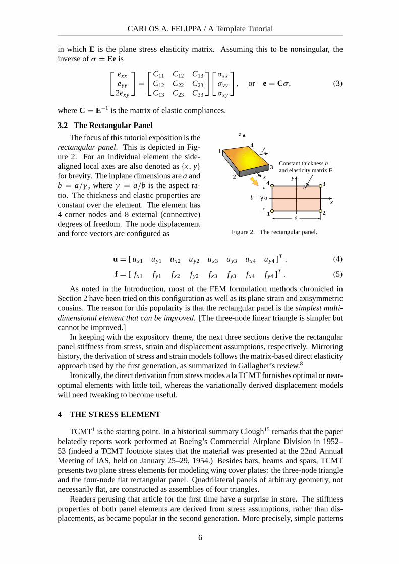
3.2 The Rectangular Panel
The focus of this tutorial exposition is therectangular panel. This is depicted in Fig-ure 2. For an individual element the side-aligned local axes are also denoted as {x, y}for brevity. The inplane dimensions are a andb = a/γ , where γ = a/b is the aspect ra-tio. The thickness and elastic properties areconstant over the element. The element has4 corner nodes and 8 external (connective)degrees of freedom. The node displacementand force vectors are configured as
1 2
34
a
x
x y
Constant thickness hand elasticity matrix E
y
z
1
2
3
4
b = γ a
Figure 2. The rectangular panel.
u = [ ux1 uy1 ux2 uy2 ux3 uy3 ux4 uy4 ]T , (4)
f = [ fx1 fy1 fx2 fy2 fx3 fy3 fx4 fy4 ]T . (5)
As noted in the Introduction, most of the FEM formulation methods chronicled inSection 2 have been tried on this configuration as well as its plane strain and axisymmetriccousins. The reason for this popularity is that the rectangular panel is the simplest multi-dimensional element that can be improved. [The three-node linear triangle is simpler butcannot be improved.]
In keeping with the expository theme, the next three sections derive the rectangularpanel stiffness from stress, strain and displacement assumptions, respectively. Mirroringhistory, the derivation of stress and strain models follows the matrix-based direct elasticityapproach used by the first generation, as summarized in Gallagher’s review.8
Ironically, the direct derivation from stress modes a la TCMT furnishes optimal or near-optimal elements with little toil, whereas the variationally derived displacement modelswill need tweaking to become useful.
4 THE STRESS ELEMENT
TCMT1 is the starting point. In a historical summary Clough15 remarks that the paperbelatedly reports work performed at Boeing’s Commercial Airplane Division in 1952–53 (indeed a TCMT footnote states that the material was presented at the 22nd AnnualMeeting of IAS, held on January 25–29, 1954.) Besides bars, beams and spars, TCMTpresents two plane stress elements for modeling wing cover plates: the three-node triangleand the four-node flat rectangular panel. Quadrilateral panels of arbitrary geometry, notnecessarily flat, are constructed as assemblies of four triangles.
Readers perusing that article for the first time have a surprise in store. The stiffnessproperties of both panel elements are derived from stress assumptions, rather than dis-placements, as became popular in the second generation. More precisely, simple patterns
6

COMPUTATIONAL MECHANICS – THEORY AND PRACTICE
of interelement boundary tractions (a.k.a. stress flux modes) that satisfy internal equilib-rium are taken as starting point. Twenty years later Fraeijs de Veubeke59 systematicallyextended the same idea in a variational setting, to produce what he called diffusive equilib-rium elements. These are designed to weakly enforce interelement flux conservation. Thecomedy continues: mathematicians recently rediscovered flux elements, now renamed as“Discontinuous Galerkin Methods,” blessfully unaware of previous work.
The derivation below largely follows Chapter 3 of Gallagher,8 who presents a step bystep procedure for what he calls the “equivalent force” approach. The main extensionprovided here is allowing for anisotropic material.
4.1 The 5-Parameter Stress Field
Since TCMT the appropriate stress field for the rectangular panel is known to be
σxx = µ1 + µ4y
b, σyy = µ2 + µ5
x
a, σxy = µ3. (6)
The five µi are stress-amplitude parame-ters with dimension of stress. They are col-lected in the 5-vector
µ = [ µ1 µ2 µ3 µ4 µ5 ]T . (7)
The field (6) satisfies the internal equilib-rium equations (1)3 under zero body forces.Evaluation over element sides produces thetraction patterns of Figure 3, transcribed ver-batim from TCMT. Why five? On p. 813:“These load states are seen to represent uni-form and linearly varying stresses plus con-stant shear, along the plate edges. Later it willbe seen that the number of load states mustbe 2n − 3, where n = number of nodes.”
t = µ1x t = −µ y/b4 x
t = µ2y
t = µ3y
t = µ3x
t = µ5y x/a
Figure 3. Interelement boundary tractionsassociated with the stress parametersµi in (7). After TCMT, p. 812, in whichthese five patterns are called “load states.”
To establish connection to node displacements, µ is extended as
µ+ = [ µ1 µ2 µ3 µ4 µ5 µ6 µ7 µ8 ]T (8)
This array contains three dimensionless coefficients: µ6, µ7 and µ8, which define ampli-tudes of the three element rigid body modes (RBMs):
RBM1: ux=µ6a, uy=0, RBM2: ux=0, uy=µ7b, RBM3: ux=−µ8 y, uy=µ8x . (9)
These modes produce zero stress. The foregoing relations may be recast in matrixform:
σ = N µ = N+µ+, N = 1 0 0 y
b 0
0 1 0 0 xa
0 0 1 0 0
, N+ =
1 0 0 y
b 0 0 0 0
0 1 0 0 xa 0 0 0
0 0 1 0 0 0 0 0
. (10)
The boundary traction patterns of Figure 3 are converted to node forces by statics. Thisyields
f = A µ, AT = 12 h
−b 0 b 0 b 0 −b 00 −a 0 −a 0 a 0 a
−a −b −a b a b a −b16 b 0 − 1
6 b 0 16 b 0 − 1
6 b 00 1
6 a 0 − 16 a 0 1
6 a 0 − 16 a
. (11)
7

CARLOS A. FELIPPA / A Template Tutorial
Matrix A is the equilibrium matrix, also known as the leverage matrix in the FEMliterature. When restricted to constant stress states (the first three columns of A), it is calleda force-lumping matrix and denoted by L in the Free Formulation of Bergan.41,42,58,60–65
4.2 The Generalized Stiffness
Integrating the complementary energy density U∗ = 12σT Cσ over the element volume
V and identifying U ∗ = ∫V e U∗ dV with 1
2µT Fµµ yields the 5 × 5 flexibility matrix Fµ
in terms of the stress parameters. Its inverse is the generalized stiffness matrix Sµ = F−1µ :
Fµ = V
C11 C12 C13 0 0C12 C22 C23 0 0C13 C23 C33 0 00 0 0 1
12 C11 00 0 0 0 1
12 C22
, Sµ = 1
V
E11 E12 E13 0 0E12 E22 E23 0 0E13 E23 E33 0 00 0 0 12C−1
11 00 0 0 0 12C−1
22
,
(12)
in which V = abh is the volume of the element.
4.3 The Physical Stiffness
Integration of the slave strain field e = E−1σ = CN+µ+ produces the displacementfield
ux (x, y) = µ6a+ 18ω6 + (µ1C11+µ2C12+µ3C13)x+( 1
2 (µ1C13+µ2C23+µ3C33) − µ8)y
+ 12 (µ5/a)C12x2 + (µ4/b)C11xy + 1
2
((µ4/b)C13 − (µ5/a)C22
)y2,
uy(x, y) = µ7b + 18ω7 + ( 1
2 (µ1C13+µ2C23+µ3C33)+µ8)x+(µ1C12+µ2C22+µ3C23)y
+ 12
((µ5/a)C23 − (µ4/b)C11
)x2 + (µ5/a)C22xy + 1
2 (µ4/b)C12 y2.
(13)
with ω6 = −b2C13µ4/b + (b2C22−a2C12)(µ5/a) and ω7 = (a2C11−b2C12)(µ4/b) −a2C23µ5/a. The constant terms in ux and uy , which do not affect strains and stresses,have been adjusted to get relatively simple terms in columns 4 through 8 of the matrixT+ below. Physically, (13) aligns the bending deformation patterns along the {x, y} axes.Evaluating (13) at the nodes we obtain the matrix that connects node displacements tostress parameters: u = T+µ+, where
T+= 14
−2aC11 − bC13 −2aC12 − bC23 −2aC13 − bC33 aC11 0 4a 0 2b−2bC12 − aC13 −2bC22 − aC23 −2bC23 − aC33 0 bC22 0 4b −2a
2aC11 − bC13 2aC12 − bC23 2aC13 − bC33 −aC11 0 4a 0 2b−2bC12 + aC13 −2bC22 + aC23 −2bC23 + aC33 0 −bC22 0 4b 2a
2aC11 + bC13 2aC12 + bC23 2aC13 + bC33 aC11 0 4a 0 −2b2bC12 + aC13 2bC22 + aC23 2bC23 + aC33 0 bC22 0 4b 2a
−2aC11 + bC13 −2aC12 + bC23 −2aC13 + bC33 −aC11 0 4a 0 −2b2bC12 − aC13 2bC22 − aC23 2bC23 − aC33 0 −bC22 0 4b −2a
(14)
The determinant of T+ is a4b4C11C22 det(C), so T+ is invertible if a �= 0, b �= 0,
8

COMPUTATIONAL MECHANICS – THEORY AND PRACTICE
Constitutive
µ = S χ
Equilibrium
Kinematic+Constitutive
u f
µ, µ
f = A µ
µ = U u
χ = A uu =T µ
f = AU u = K u
+
+
+
σ
EquilibriumKinematic
u f
µ, µ
f = A µ
f = AS A u = K u
+
σ
χ
T
T
µ
µ
(a) Direct derivation a la TCMT (b) Energy derivation
Figure 4. Derivation of the stress-assumed rectangular panel stiffness.Left side shows derivation bypassing energy methods.
C11 �= 0, C22 �= 0 and C is nonsingular. Inversion yields µ+ = U+u, where
U+ = T−1+ = 1
ab
U11 U12 U13 U14 U15 U16 U17 U18
U21 U22 U23 U24 U25 U26 U27 U28
U31 U32 U33 U34 U35 U36 U37 U38
bC−111 0 −bC−1
11 0 bC−111 0 −bC−1
11 00 aC−1
22 0 −aC−122 0 aC−1
22 0 −aC−122
14 b 0 1
4 b 0 14 b 0 1
4 b 00 1
4 a 0 14 a 0 1
4 a 0 14 a
14 a − 1
4 b 14 a 1
4 b − 14 a 1
4 b − 14 a − 1
4 b
,
(15)
in which U11 = − 12 (bE11+aE13), U12 = − 1
2 (aE12+bE13), U13 = 12 (bE11−aE13),
U14 = − 12 (aE12−bE13), U15 = 1
2 (bE11+aE13), U16 = 12 (aE12+bE13), U17 =
− 12 (bE11−aE13), U18 = 1
2 (aE12−bE13), U21=− 12 (bE12+aE23), U22=− 1
2 (aE22+bE23),U23 = 1
2 (bE12−aE23), U24 = − 12 (aE22−bE23), U25 = 1
2 (bE12+aE23), U26 =12 (aE22+bE23), U27 = − 1
2 (bE12−aE23), U28 = 12 (aE22−bE23), U31 = − 1
2 (bE13+aE33),U32 = − 1
2 (aE23+bE33), U33 = 12 (bE13−aE33), U34 = − 1
2 (aE23−bE33), U35 =12 (bE13+aE33), U36 = 1
2 (aE23+bE33), U37 = − 12 (bE13−aE33) and U38 =
12 (aE23−bE33). The stress-displacement matrix U that relates stress parameters to dis-placements: µ = U u, is obtained by extracting the first five rows of U+:
U = 1
ab
U11 U12 U13 U14 U15 U16 U17 U18
U21 U22 U23 U24 U25 U26 U27 U28
U31 U32 U33 U34 U35 U36 U37 U38
bC−111 0 −bC−1
11 0 bC−111 0 −bC−1
11 00 aC−1
22 0 −aC−122 0 aC−1
22 0 −aC−122
= Sµ AT .
(16)
The relation U = SµAT can be checked directly. For this element it can be proven tohold by energy methods, but that was not obvious in 1952. It must have been a relief whenthe element stiffness came out symmetric. As Gallagher8 remarks on p. 22, symmetryis the exception rather than the rule for more general geometric configurations. Thatcomplication proved a big boost for the energy and variational methods of the secondgeneration.
The physical stiffness Kσ relates f = Kσ u, where the σ subscript flags the stress
9

CARLOS A. FELIPPA / A Template Tutorial
element. Combining f = A µ and µ = U u = Sµ AT u yields
Kσ = A U = A Sµ AT . (17)
Figure 4 summarizes the foregoing derivation steps. Note that one can bypass the calcu-lation of the generalized stiffness Sµ if so desired, as diagramed on the left of that figure.This is convenient for presentation to students without a background on energy methods.
Note that the displacement field (13) contains quadratic terms if µ4 or µ5 are nonzero.Hence the element is nonconforming. This is acknowledged but dismissed as innocuouson p. 814 of TCMT.
5 THE STRAIN ELEMENT
A strain-assumed element can be developed through an entirely analogous procedure.The counterpart of (6) is
exx = χ1 + χ4y
b, eyy = χ2 + χ5
x
a, 2exy = χ3. (18)
where the χi are dimensionless strain-amplitude parameters. They are collected in the5-vector
χ = [ χ1 χ2 χ3 χ4 χ5 ]T . (19)
An extended vector is constructed by appending the RBM amplitudes
χ+ = [ χ1 χ2 χ3 χ4 χ5 χ6 χ7 χ8 ]T . (20)
in which χ6, χ7 and χ8 are defined a a manner similar to (9). Note that e = Nχ = N+χ+where N and N+ are defined in (10). Integrating the strains yields the displacement field
ux (x, y) = χ6 + χ8 y + (χ1 + χ4/b)xy − 12 (χ5/a)y2,
uy(x, y) = χ7 + (χ3 − χ8)x + χ2 y − 12 (χ4/b)x2 + (χ5/a)xy.
(21)
Evaluating at the nodes and inverting yields χ+ = B+u where
B+ = 1
8ab
−4b 0 4b 0 4b 0 −4b 00 −4a 0 −4a 0 4a 0 4a
−4a −4b −4a 4b 4a 4b 4a −4b8b 0 −8b 0 8b 0 −8b 00 8a 0 −8a 0 8a 0 −8a
2ab b2 2ab −b2 2ab b2 2ab −b2
a2 2ab −a2 2ab a2 2ab −a2 2ab−4a 0 −4a 0 4a 0 4a 0
(22)
from which we extract the first five rows to get the strain-displacement matrix relatingχ = Bχu:
Bχ = h
2V
−b 0 b 0 b 0 −b 00 −a 0 −a 0 a 0 a
−a −b −a b a b a −b2b 0 −2b 0 2b 0 −2b 00 2a 0 −2a 0 2a 0 −2a
(23)
10

COMPUTATIONAL MECHANICS – THEORY AND PRACTICE
Kinematicχ = B u χ = B uu = B χ Constitutive+
Equilibrium
u f
χ, χ +f = B V D E χ + +
+
T
−1
Constitutive
µ =V D E χ = S χ
EquilibriumKinematic
u f
µ
f = B µ
f = B S B u = K u eT
T
χχ, χ+
χχ
χ
χ
χ χ χ
A
f = B V D E B u = K u
+T
e
χχ A
(a) Direct derivation as per Ref. 8 (b) Energy derivation
Figure 5. Derivation of the strain-assumed rectangular panel stiffness.Left diagram shows derivation bypassing energy methods.
For use below we note the following relation between the transformation matrices of thestress and strain elements
AT = V DA Bχ , Bχ = 1
VD−1
A AT , DA =
1 0 0 0 00 1 0 0 00 0 1 0 00 0 0 1
12 00 0 0 0 1
12
=
[I3 00 1
12 I2
]= DT
A.
(24)
From (11) the lumping of the slave stress field Ee = ENχ to node forces can be workedout to be
f = AE+χ = V BTχ DAE+χ, with E+ =
E11 E12 E13 0 0E12 E22 E23 0 0E13 E23 E33 0 00 0 0 E11 00 0 0 0 E22
(25)
Combining previous equations, the physical element stiffness is
Ke = V BTχ DAE+Bχ = BT
χ KχBχ , with Kχ = V DAE+. (26)
Here Kχ denotes the generalized stiffness in terms of χ. This matrix may be ob-tained also from standard energy arguments: the strain energy density is U = 1
2χT Eχ.Integrating over the element volume: U = ∫
V e U dV and identifying with 12χT Kχχ gives
Kχ = V DAE+ = V
E11 E12 E13 0 0E12 E22 E23 0 0E13 E23 E33 0 00 0 0 1
12 E11 00 0 0 0 1
12 E22
(27)
Figure 5 summarizes the foregoing derivation steps. The direct step from χ to f onthe left is more difficult to explain to students than the step from u to µ in Figure 4. Theenergy based formulation shown on the right of Figure 5 tends to be more palatable.
11

CARLOS A. FELIPPA / A Template Tutorial
6 THE CONFORMING DISPLACEMENT ELEMENT
This derivation of the assumed-displacement element starts from a conforming dis-placement field that enforces linear edge displacements. Using the matrix notation ofFelippa and Clough66 for Irons’ isoparametric formulation25 specialized to the rectangle,the displacement field is bilinearly interpolated as
[ux (x, y)
uy(x, y)
]= 1
2
[ −a 0 a 0 a 0 −a 00 −b 0 −b 0 b 0 b
]
14 (1 − ξ)(1 − η)14 (1 + ξ)(1 − η)14 (1 + ξ)(1 + η)14 (1 − ξ)(1 + η)
, (28)
where ξ = 2x/a and η = 2y/b are the dimensionless quadrilateral coordinates runningfrom −1 to 1. The derivation based on the minimum potential energy principle is standardtextbook material and only the final result is presented here:
Ku = BTu KqBu, with Kq = 1
V
E11 E12 E13 0 0E12 E22 E23 0 0E13 E23 E33 0 00 0 0 Q11 Q12
0 0 0 Q12 Q22
, (29)
in which Bu = AT as given by (11) and
Q11 = 12b2 E11 + a2 E33
ab3h, Q12 = 12
(E13
a2h+ E23
b2h
), Q22 = 12
a2 E22 + b2 E33
a3bh(30)
This model has a checkered history. It was first derived as a rectangular panel withedge reinforcements (omitted here) by Argyris in his 1954 Aircraft Engineering series; seepp. 49–52 of the Butterworths reprint.5 Argyris used bilinear displacement interpolationin Cartesian coordinates. After much flailing, a conforming generalization to arbitrarygeometry was published in 1964 by Taig and Kerr67 using quadrilateral-fitted coordinatescalled {ξ, η} but running from 0 to 1. This paper cites an 1961 English Electric Aircraftinternal report as original source but Irons and Ahmad25 comment in their reference [108]that the work goes back to 1957.) Irons, who was aware of Taig’s work while at RollsRoyce, created the seminal isoparametric family as a far-reaching extension upon movingto Swansea.21–24
7 TEMPLATES
7.1 Stiffness DecompositionThe stiffnesses Kσ , Ke and Ku derived in the foregoing three Sections do not appear to
have much in common. Indeed if one looks at just the matrix entries no pattern is readilyseen. Closer examination reveals, however, that they are instances of the algebraic form
K = Kb + Kh = V HTc EHc + V HT
h WT RWHh, (31)
where V = abh is the element volume and
Hc = 1
2ab
[ −b 0 b 0 b 0 −b 00 −a 0 −a 0 a 0 a
−a −b −a b a b a −b
],
Hh = 12
[1 0 −1 0 1 0 −1 00 1 0 −1 0 1 0 −1
],
W =[
1/a 00 1/b
], R =
[R11 R12
R12 R22
].
(32)
12

COMPUTATIONAL MECHANICS – THEORY AND PRACTICE
Formulation dependent (W is independent for rectangles)
K = V H E H + V H W R W H
Formulation independent
(e)c cT T T
8x8 8x3 3x3 3x8 8x2 2x2 2x2 2x2 2x8
hh
Figure 6. The template for the rectangular panel, illustratingformulation dependent and independent parts.
Matrices Hc and Hh are identical for the three models. The generalized bending rigidityR is formulation dependent. Matrix W is a “higher-order-mode weighting matrix,” hencethe notation. For rectangular panels W is diagonal and formulation independent. For morecomplex geometries discussed in the Appendix and in the sequel3 W may be formulation-adjusted to make R simpler.
For the stress, strain and displacement models R becomes Rσ , Re and Ru , respectively,where
Rσ = 13
[C−1
11 00 C−1
22
], Re = 1
3
[E11 00 E22
], Ru = 1
3
E11 + a2 E33
b2bE13
a + aE23b
bE13a + aE23
b E22 + b2 E33
a2
(33)
But we are not in fact restricted to these. Other expressions for R would yield other K.These are possible, although not necessarily useful, stiffnesses for the rectangular panel ifR is symmetric and positive definite, and if its entries have physical dimensions of elasticmoduli. Further if E13 = E23 = 0 we set R12 = 0. The key discovery is that the elementformulation affects only part of the stiffness expression, as highlighted in Figure 6.
7.2 Template Terminology
The algebraic form characterized by (31) and (32) is called a finite element stiffnesstemplate, or template for short.
Matrices Kb and Kh are called the basic and higher-order stiffness matrix, respec-tively, in accordance with the fundamental decomposition of the Free Formulation.41,42,58–65
These two matrices play different and complementary roles.The basic stiffness Kb takes care of consistency and mixability. In the Free Formulation
a restatement of (31) is preferred:
Kb = V −1 L E LT , (34)
where L = Hc/V is called the force lumping matrix, or simply lumping matrix.The higher order stiffness Kh is a stabilization term that provides the correct rank and
may be adjusted for accuracy. This matrix is orthogonal to rigid body motions and constantstrain states. To verify the claim for this particular template introduce the following 8 × 6
13
CARLOS A. FELIPPA / A Template Tutorial
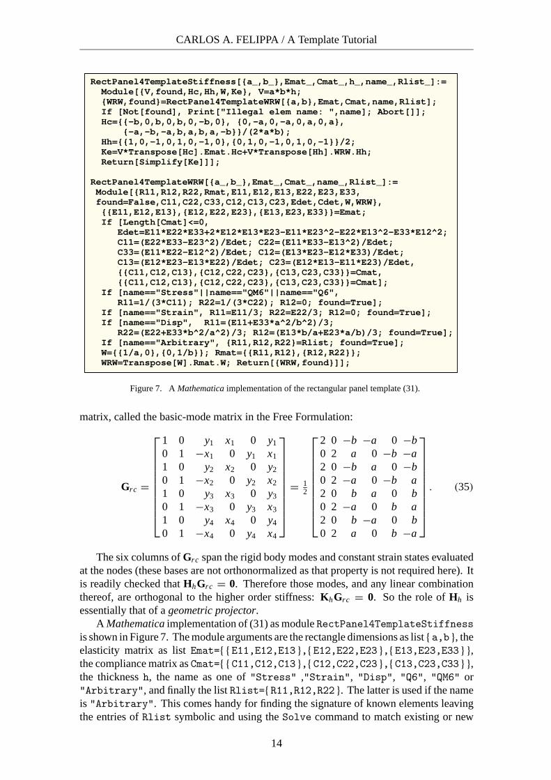
RectPanel4TemplateStiffness[{a_,b_},Emat_,Cmat_,h_,name_,Rlist_]:= Module[{V,found,Hc,Hh,W,Ke}, V=a*b*h; {WRW,found}=RectPanel4TemplateWRW[{a,b},Emat,Cmat,name,Rlist]; If [Not[found], Print["Illegal elem name: ",name]; Abort[]]; Hc={{-b,0,b,0,b,0,-b,0}, {0,-a,0,-a,0,a,0,a}, {-a,-b,-a,b,a,b,a,-b}}/(2*a*b); Hh={{1,0,-1,0,1,0,-1,0},{0,1,0,-1,0,1,0,-1}}/2; Ke=V*Transpose[Hc].Emat.Hc+V*Transpose[Hh].WRW.Hh; Return[Simplify[Ke]]]; RectPanel4TemplateWRW[{a_,b_},Emat_,Cmat_,name_,Rlist_]:= Module[{R11,R12,R22,Rmat,E11,E12,E13,E22,E23,E33, found=False,C11,C22,C33,C12,C13,C23,Edet,Cdet,W,WRW}, {{E11,E12,E13},{E12,E22,E23},{E13,E23,E33}}=Emat; If [Length[Cmat]<=0, Edet=E11*E22*E33+2*E12*E13*E23-E11*E23^2-E22*E13^2-E33*E12^2; C11=(E22*E33-E23^2)/Edet; C22=(E11*E33-E13^2)/Edet; C33=(E11*E22-E12^2)/Edet; C12=(E13*E23-E12*E33)/Edet; C13=(E12*E23-E13*E22)/Edet; C23=(E12*E13-E11*E23)/Edet, {{C11,C12,C13},{C12,C22,C23},{C13,C23,C33}}=Cmat, {{C11,C12,C13},{C12,C22,C23},{C13,C23,C33}}=Cmat]; If [name=="Stress"||name=="QM6"||name=="Q6", R11=1/(3*C11); R22=1/(3*C22); R12=0; found=True]; If [name=="Strain", R11=E11/3; R22=E22/3; R12=0; found=True]; If [name=="Disp", R11=(E11+E33*a^2/b^2)/3; R22=(E22+E33*b^2/a^2)/3; R12=(E13*b/a+E23*a/b)/3; found=True]; If [name=="Arbitrary", {R11,R12,R22}=Rlist; found=True]; W={{1/a,0},{0,1/b}}; Rmat={{R11,R12},{R12,R22}}; WRW=Transpose[W].Rmat.W; Return[{WRW,found}]];
Figure 7. A Mathematica implementation of the rectangular panel template (31).
matrix, called the basic-mode matrix in the Free Formulation:
Grc =
1 0 y1 x1 0 y1
0 1 −x1 0 y1 x1
1 0 y2 x2 0 y2
0 1 −x2 0 y2 x2
1 0 y3 x3 0 y3
0 1 −x3 0 y3 x3
1 0 y4 x4 0 y4
0 1 −x4 0 y4 x4
= 12
2 0 −b −a 0 −b0 2 a 0 −b −a2 0 −b a 0 −b0 2 −a 0 −b a2 0 b a 0 b0 2 −a 0 b a2 0 b −a 0 b0 2 a 0 b −a
. (35)
The six columns of Grc span the rigid body modes and constant strain states evaluatedat the nodes (these bases are not orthonormalized as that property is not required here). Itis readily checked that HhGrc = 0. Therefore those modes, and any linear combinationthereof, are orthogonal to the higher order stiffness: KhGrc = 0. So the role of Hh isessentially that of a geometric projector.
A Mathematica implementation of (31) as module RectPanel4TemplateStiffnessis shown in Figure 7. The module arguments are the rectangle dimensions as list { a,b }, theelasticity matrix as list Emat={ { E11,E12,E13 },{ E12,E22,E23 },{ E13,E23,E33 } },the compliance matrix as Cmat={ { C11,C12,C13 },{ C12,C22,C23 },{ C13,C23,C33 } },the thickness h, the name as one of "Stress" ,"Strain", "Disp", "Q6", "QM6" or"Arbitrary", and finally the list Rlist={ R11,R12,R22 }. The latter is used if the nameis "Arbitrary". This comes handy for finding the signature of known elements leavingthe entries of Rlist symbolic and using the Solve command to match existing or new
14

COMPUTATIONAL MECHANICS – THEORY AND PRACTICE
Table 1. A Clone Gallery
Name Description Clones and sources
StressRP 5-stress-mode element Direct derivation: TCMT1, Gallagher8
(a.k.a. BORP) of Section 4 Pian 5-mode stress hybrid27,26,29
Wilson-Taylor-Doherty-Ghaboussi Q668
Taylor-Wilson-Beresford QM669
Belytschko-Liu-Engelmann QBI70
SRI of iso-P with E split as per (54)
StrainRP 5-strain-mode element MacNeal QUAD439,71
of Section 5 SRI of iso-P with E split as per (56)
DispRP Bilinear iso-P element Argyris5 as edge stiffened rectangular panelof Section 6 Taig-Kerr67 as specialized quadrilateral
Note 1: Many plane stress models listed above were derived for quadrilateral geometries,and a few as membrane component of shells. The right-hand-column classificationonly pertains to the rectangular panel specialization. For example,Q6 and QM6 differ for non-parallelogram shapes.
Note 2: Instances of the stress-hybrid and displacement-bubble-function “futile families”studied in Section 11 are omitted, as they lack practical value.
Note 3: Post-1990 clones (e.g. EAS54) omitted to save space. See Lautersztajn andSamuelsson72 for a recent survey.
elements. If Cmat is supplied as the empty list { }, the compliance matrix is calculatedinternally as inverse of Emat.
The module returns the 8 × 8 stiffness matrix Ke as function value. To get the basicstiffness Kb only, call with name = "Arbitrary" and Rlist={ 0,0,0 }.7.3 Requirements
An acceptable template fulfills four conditions: (C) consistency, (S) stability (correctrank), (I) observer invariance and (P) parametrization. These are discussed at lengthin other papers.73–79 Conditions (C) and (S) are imposed to ensure convergence as themesh size is reduced by enforcing a priori satisfaction of the Individual Element Test(IET) of Bergan and Hanssen.56,57 Condition (P) means that the template contains freeparameters or free matrix entries. In the case of (31), the simplest choice of parametersare the entries R11, R12, R22 themselves. To fulfill stability, R11 > 0, R22 > 0 andR11 R22 − R2
12 > 0. Parametrization facilitates performance optimization as well as tuningelements, or combinations of elements, to fulfill specific needs.
Using the IET as departure point it is not difficult to show80 that (31), under thestated restrictions on R, includes all stiffnesses that satisfy the IET and stability. Observerinvariance is a moot point for this element since {x, y} are side aligned. Thus (31) is infact a universal template for the rectangular panel.
7.4 Instances, Signatures, Clones
Setting the free parameters to specific values yields element instances. The set offree parameters is called the template signature, a term introduced in previous papers.77,78
Borrowing terminology from biogenetics, the signature may be viewed as an “elementDNA” that uniquely characterizes it as an individual entity. Elements derived by differenttechniques that share the same signature are called clones.
15

CARLOS A. FELIPPA / A Template Tutorial
1 2
34x
M M
����
a
b = a/γ
b
h
Cross section
y
y
zxz
yx x
Figure 8. Constant-moment inplane-bending test along the x side dimension.
One of the “template services” is automatic identification of clones. If two elementsfitting the template (31) share R11, R12 and R22, they are clones. Inasmuch as most FEMformulation schemes have been tried on the rectangular panel, it should come as no surprisethat there are many clones, particularly of the stress element. Those published before 1990are collected in Table 1. For example, the incompatible mode element Q6 of Wilson etal.68 is a clone of StressRP. The version QM6 of Taylor et al.69 which passes the patch testfor arbitrary geometries, reduces to Q6 for rectangular and parallelogram shapes. Even forthis simple geometry recognition of some of the coalescences took some time, as recentlynarrated by Pian.29
8 FINDING THE BEST
An universal template is nice to have. The obvious question arises: among the infinityof elements that it can generate, is there a best one? By construction all instances verifyexactly the IET for rigid body modes and uniform strain states. Hence the optimalitycriterion must rely on higher order patch tests.
8.1 The Bending Tests
The obvious tests involve response to in-plane bending along the side directions. Thisleads to comparisons in the form of energy ratios. These have been used since 1984 totune up the higher order stiffness of triangular elements.58–62,81 An extension introducedin this article is consideration of arbitrary anisotropic material. All symbolic calculationswere carried out with Mathematica.
The x bending test is depicted in Figure 8. A Bernoulli-Euler plane beam of thinrectangular cross-section with height b and thickness h (normal to the plane of the figure)is bent under applied end moments Mx . The beam is fabricated of anisotropic materialwith the stress-strain law σ = Ee of (2)2. Except for possible end effects the exact solutionof the beam problem (from both the theory-of-elasticity and beam-theory standpoints) isa constant bending moment M(x) = Mx along the span. The associated stress field isσxx = −Mx y/Ib, σyy = σxy = 0, where Ib = 1
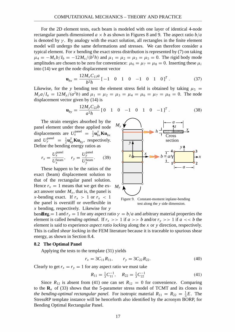
12 hb3.For the y bending test, depicted in Figure 9, the beam cross section has height a and
thickness h, and is subjected to end moments My . The exact solution is M(y) = My .The associated stress field is σyy = My x/Ia and σxx = σxy = 0, where Ia = 1
12 ha3.For comparing with the FEM discretizations below, the internal (complementary) energiestaken up by beam segments of lengths a and b in the configurations of Figures 8 and 9,respectively, are
U beamx = 6aC11 M2
x
b3h, U beam
y = 6bC22 M2y
a3h(36)
16
COMPUTATIONAL MECHANICS – THEORY AND PRACTICE
For the 2D element tests, each beam is modeled with one layer of identical 4-noderectangular panels dimensioned a × b as shown in Figures 8 and 9. The aspect ratio b/ais denoted by γ . By analogy with the exact solution, all rectangles in the finite elementmodel will undergo the same deformations and stresses. We can therefore consider atypical element. For x bending the exact stress distribution is represented by (7) on takingµ4 = −Mx b/Ib = −12Mx/(b2h) and µ1 = µ2 = µ3 = µ5 = 0. The rigid body modeamplitudes are chosen to be zero for convenience: µ6 = µ7 = µ8 = 0. Inserting these µi
into (14) we get the node displacement vector
ubx = 12Mx C11a
b2h[ −1 0 1 0 −1 0 1 0 ]T . (37)
Likewise, for the y bending test the element stress field is obtained by taking µ5 =Mya/Ia = 12My/(a2h) and µ1 = µ2 = µ3 = µ4 = µ6 = µ7 = µ8 = 0. The nodedisplacement vector given by (14) is
uby = 12MyC22b
a2h[ 0 1 0 −1 0 1 0 −1 ]T . (38)
The strain energies absorbed by thepanel element under these applied nodedisplacements are U panel
x = 12 uT
bx Kubx
and U panely = 1
2 uTbyKuby , respectively.
Define the bending energy ratios as
rx = U panelx
U beamx
, ry = U panely
U beamy
. (39)
These happen to be the ratios of theexact (beam) displacement solution tothat of the rectangular panel solution.Hence rx = 1 means that we get the ex-act answer under Mx , that is, the panel isx-bending exact. If rx > 1 or rx < 1the panel is overstiff or overflexible inx bending, respectively. Likewise for ybending.
1 2
34
a
a
b = a/γ x
hCross section
x
������z
My
My
y
xz
y
Figure 9. Constant-moment inplane-bendingtest along the y side dimension.
If rx = 1 and ry = 1 for any aspect ratio γ = b/a and arbitrary material properties theelement is called bending optimal. If rx >> 1 if a >> b and/or ry >> 1 if a << b theelement is said to experience aspect ratio locking along the x or y direction, respectively.This is called shear locking in the FEM literature because it is traceable to spurious shearenergy, as shown in Section 8.4.
8.2 The Optimal PanelApplying the tests to the template (31) yields
rx = 3C11 R11, ry = 3C22 R22. (40)
Clearly to get rx = ry = 1 for any aspect ratio we must take
R11 = 13 C−1
11 , R22 = 13 C−1
22 (41)
Since R12 is absent from (41) one can set R12 = 0 for convenience. Comparingto the Rσ of (33) shows that the 5-parameter stress model of TCMT and its clones isthe bending-optimal rectangular panel. For isotropic material R11 = R22 = 1
3 E . TheStressRP template instance will be henceforth also identified by the acronym BORP, forBending Optimal Rectangular Panel.
17

CARLOS A. FELIPPA / A Template Tutorial
8.3 The Strain Element Does Not Lock
It is interesting to apply the result (40) to other template instances. The StrainRPelement generated by the Re of (33) gives
rx = C11 E11, ry = C22 E22. (42)
If the material is isotropic, C11 = C22 = 1/E and E11 = E22 = E/(1 − ν2). Thisyields rx = ry = 1/(1 − ν2), which varies between 1 and 4/3. For an orthotropic bodywith principal material axes aligned with the rectangle sides, E11 = E1/(1 − ν12ν21),E22 = E2/(1 − ν12ν21), C11 = 1/E1, C22 = 1/E2, and rx = ry = 1/(1 − ν12ν21). Theseare independent of the aspect ratio γ . Consequently StrainRP and its clones do not lock,although the element is not generally optimal. Note that if C11 E11 and/or C22 E22 differwidely from 1, as may happen in highly anisotropic materials, the bending performancewill be poor. The example of Section 12.2 displays this vividly.
8.4 But the Displacement Element Does
Instance DispRP is generated by the Ru of (33). Inserting its entries into (40) we get
rx = C11(E11 + E33γ2) = (E22 E33 − E2
23)(E11 + E33γ2)
det(E),
ry = C22(E22 + E33γ−2) = (E11 E33 − E2
13)(E22 + E33γ−2)
det(E).
(43)
in which det(E) = E11 E22 E33 + 2E12 E13 E23 − E11 E223 − E22 E2
13 − E33 E212. For an
isotropic material
rx = 2 + γ 2(1 − ν)
2(1 − ν2), ry = 1 + 2γ 2 − ν
2γ 2(1 − ν2). (44)
These relations clearly indicate aspect ratio locking for bending along the longest sidedimension. For instance if ν = 0 and a = 10b , whence γ = a/b = 10, then rx = 51 andDispRP is over 50 times stiffer in x bending than the Bernoulli-Euler beam element. Theexpression (43) makes clear that locking happens for any material law as long as E33 �= 0.Since this is the shear modulus, the name shear locking used in the FEM literature isjustified.
8.5 Multiple Element Layers
Results of the energy bending test can be readily extended to predict the behavior of 2n(n = 1, 2, . . .) identical layers of elements symmetrically placed through the beam height.If 2n layers are placed along the y direction in the configuration of Figure 8 and γ staysthe same, the energy ratio becomes
r (2n)x = 22n − 1 + rx
22n, (45)
where rx is the ratio (40) for one layer. If rx ≡ 1, r2nx ≡ 1 so bending exactness is
maintained, as can be expected. For example, if n = 1 (two element layers), r (2)x =
(3 + rx )/4. The same result holds for ry if 2n layers are placed along the x direction inthe configuration of Figure 9.
18

COMPUTATIONAL MECHANICS – THEORY AND PRACTICE
��
1
4 3
2
b = a/γ
h
Cross section
y
z x1 2
ux1
uy1
ux 2
uy2
θ2
θ1−−
−
− −
E, A, I zza = La
morphingx
y
Figure 10. Morphing a 8-DOF rectangular panel unit to a6-DOF beam-column element in the x direction.
9 MORPHING TO BEAM-COLUMN
Morphing means transforming an individual element or macroelement into a simplermodel using kinematic constraints. Often the simpler element has lower dimensionality.For example a plate bending macroelement may be morphed to a Bernoulli-Euler beam or toa torqued shaft.79 To illustrate the idea consider morphing the rectangular panel of Figure 10into the two-node beam-column element shown on the right of that Figure. The length,cross sectional area and moment of inertia of the beam-column element, respectively, aredenoted by L = a, A = bh and Izz = b3h/12 = a3h/(12γ 3), respectively.
The transformation between the freedoms of the panel and those of the beam-columnis
uR =
ux1
uy1
ux2
uy2
ux3
uy3
ux4
uy4
=
1 0 12 b 0 0 0
0 1 0 0 0 00 0 0 1 0 1
2 b0 0 0 0 1 00 0 0 1 0 − 1
2 b0 0 0 0 1 01 0 − 1
2 b 0 0 00 1 0 0 0 0
ux1
u y1
θ1
ux2
u y2
θ2
= Tm um . (46)
where a superposed bar distinguishes the beam-column freedoms grouped in array um .As source select StressRP fabricated of isotropic material. The morphed beam-columnelement stiffness is
Km = TTm Kσ Tm = E
L
A 0 0 −A 0 00 12c22 Izz/L2 6c23 Izz/L 0 −12c22 Izz/L2 6c23 Izz/L0 6c23 Izz/L 4c33 Izz 0 −6c23 Izz/L 4c33 Izz
−A 0 0 A 0 00 12c22 Izz/L2 6c23 Izz/L 0 −12c22 Izz/L2 6c23 Izz/L0 6c23 Izz/L 4c33 Izz 0 −6c23 Izz/L 4c33 Izz
(47)
in which c22 = c23 = 12γ 2/(1 + ν), and c33 = 1
4 (1 + 3c22). The entries in rows/columns1 and 4 form the well known two-node bar stiffness. Those in rows and columns 2, 3, 5and 6 are dimensionally homogeneous to those of a plane beam, and may be grouped intothe following matrix configuration:
Kbeamm = E Izz
L
0 0 0 00 1 0 −10 0 0 00 −1 0 1
+ βm
12/L2 6/L −12/L2 6/L6/L 3 −6/L 3
−12/L2 −6/L 12/L2 −6/L6/L 3 −6/L 3
(48)
19
CARLOS A. FELIPPA / A Template Tutorial
where βm = c22 = c23 = 12γ 2/(1 + ν). But (48), with βm replaced by a free parameter β,
happens to be the universal template of a prismatic plane beam.73 Mass-stiffness templatecombinations have been studied for dynamics and vibration using Fourier methods.82,83
The basic stiffness on the left characterizes the pure-bending symmetric responseto a uniform moment, whereas the higher-order stiffness on the right characterizes theantisymmetric response to a linearly-varying, bending moment of zero mean. For theBernoulli-Euler beam constructed with cubic shape functions, β = 1. For the Timoshenkobeam, the exact equilibrium model developed in §5.6 of Przemieniecki7 is matched byβ = βC0 = 1/(1 + φ), φ = 12E Iz/(G As L2), in which As = 5bh/6 is the shear area andG = 1
2 E/(1 + ν) the shear modulus. The morphed βm is always higher than βC0 for all0 ≤ ν ≤ 1
2 and aspect ratios γ > 0. This indicates that in beam-like problems involvingtransverse shear the rectangular panel will be stiffer than the exact C0 beam model. Forexample if ν = 1/4
βC0
βm= 5
2(3 + γ 2). (49)
This never exceeds 5/6 and goes to zero as γ → ∞. This reflects the fact that a4-node panel can only respond to such antisymmetric nodal motions by deforming in pureshear. The symmetric response, however, is exact for any aspect ratio γ , confirming theoptimality of StressRP (= BORP). Observe also that what was a higher order patch test onthe two-triangle mesh unit becomes a basic (constant-moment) patch test on the morphedelement. This is typical of morphing transformations that reduce spatial dimensionality.
For nonoptimal elements, one finds that the basic stiffness of the morphed beam iswrong except under very special circumstances. For example isotropic StrainRP with zeroν, or one of the SRI elements studied next.
10 A G3 DEVICE: SELECTIVE REDUCED INTEGRATION
The three canonical models of Sections 4-6 were known by the end of Generation 2.Next a third generation tool will be studied in the context of templates. Full ReducedIntegration (FRI) and Selective Reduced Integration (SRI) emerged during 1969–7284–87
as tools to “unlock” isoparametric displacement models. Initially labeled as “variationalcrimes” by Strang33 they were eventually justified through lawful association with mixedvariational methods.88–90 Both FRI and SRI turned out to be particularly useful for legacyand nonlinear codes because they allow shape function and numerical integration modulesto be reused. For the 4-node panel only SRI is considered because FRI leads to rankdeficiency: R11 = R12 = R22 = 0. Two questions can be posed:(i) Can the template (31)–(32) be reproduced for any material law by a SRI scheme?(ii) Can BORP be cloned for any material law by a SRI scheme that is independent of
the aspect ratio?As shown below, the answers are (i): yes if R12 = 0; (ii): yes.
10.1 Concept and Notation
In the FEM literature, SRI identifies a scheme for forming K as the sum of two or morematrices computed with different integration rules and different constitutive properties,within the framework of the isoparametric (iso-P) displacement model. We will focushere on a two-way constitutive decomposition. Split the plane stress constitutive matrix Einto
E = EI + EII. (50)
The iso-P displacement formulation leads to the expression K = ∫Ae h BT
u E Bu d�
where Ae is the element area and Bu the iso-P strain-displacement matrix. To apply SRI
20

COMPUTATIONAL MECHANICS – THEORY AND PRACTICE
1
4 3
2
b = a/γ
a
x
y
1
4 3
2 1
4 3
2= +E I
E IIE = E + EI II
Figure 11. Matrix split for two-way SRI.
insert the splitting (50) into E to get two integrals:
K =∫
Ae
h BTu EI Bu d� +
∫Ae
h BTu EII Bu d� = KI + KII. (51)
The two matrices in (51) are done through different numerical quadrature schemes:rule (I) for the first integral and rule (II) for the second. For the rectangular panel theisoparametric model is the 4-node bilinear element. Rules (I) and (II) will be the 1×1(one point) and 2×2 (4-point) Gauss product rules, respectively. A general split of theelasticity matrix is
E = EI + EII =[ E11 ρ1 E12ρ3 E13τ2
E12 ρ3 E22 ρ2 E23τ2
E13 τ2 E23 τ2 E33τ1
]+
[ E11(1 − ρ1) E12(1 − ρ3) E13(1 − τ2)
E12(1 − ρ3) E22(1 − ρ2) E23(1 − τ3)
E13(1 − τ2) E23(1 − τ3) E33(1 − τ1)
],
(52)
in which ρ1, ρ2, ρ3, τ1, τ2 and τ3 are dimensionless coefficients to be chosen.
10.2 The Case R12 = 0
A template with R12 = 0 and arbitrary {R11, R22} is matched by taking
ρ1 = 1 − 3R11
E11, ρ2 = 1 − 3R22
E22, τ1 = τ2 = τ3 = 1. (53)
Since ρ3 does not appear, it is convenient to set it to one to get a diagonal EII. The resultingsplit is
EI + EII =[ E11 − 3R11 E12 E13
E12 E22 − 3R22 E23
E13 E23 E33
]+
[ 3R11 0 00 3R22 00 0 0
], (54)
To get the optimal element (BORP) set R11 = 13 C−1
11 and R22 = 13 C−1
22 :
EI + EII =[ E11 − C−1
11 E12 E13
E12 E22 − C−122 E23
E13 E23 E33
]+
[ C−111 0 00 C−1
22 00 0 0
], (55)
For isotropic material this becomes
EI + EII = E
1 − ν2
[ν2 ν 0ν ν2 00 0 1
2 (1 − ν)
]+ E
[ 1 0 00 1 00 0 0
]. (56)
To match the (suboptimal) StrainRP, in which R11 = 13 E11 and R22 = 1
3 E22 the appropriatesplit is
EI + EII =[ 0 E12 E13
E12 0 E23
E13 E23 E33
]+
[ E11 0 00 E22 00 0 0
]. (57)
21
CARLOS A. FELIPPA / A Template Tutorial
For isotropic material this becomes
EI + EII = E
[ 0 ν 0ν 0 00 0 1
2 (1 − ν)
]+ E
[ 1 0 00 1 00 0 0
]. (58)
Some FEM books suggest using the dilatational (a.k.a. volumetric, bulk) elasticity law forEI . As can be seen, the recommendation is incorrect for this element.
10.3 The Case R12 �= 0
The case R12 �= 0 arises in anisotropic displacement models in which E13 �= 0 and/orE23 �= 0. Now τ2 and τ3 must verify E13γ
−1τ2 + E23γ τ3 = E13γ−1 + E23γ − 3R12.
Solve for that τi (i = 2, 3) that has an associated nonzero modulus. Note that the aspectratio γ will generally appear in the SRI rule.
This case lacks practical interest because optimality can be achieved with R12 = 0.But for DispRP an obvious solution that eliminates all aspect ratio dependent is ρ1 = ρ2 =ρ3 = τ1 = τ2 = τ3 = 0, whence EI = 0, EII = E and the fully integrated isoP element,which locks, is recovered.
10.4 Selective Directional Integration
The template can also be generated by non-Gaussian rules. For example, the followingthree-way directional split
EI +EII +EIII =[ E11 − C−1
11 E12 E13
E12 E22 − C−122 E23
E13 E23 E33
]+
[ C−111 0 00 0 00 0 0
]+
[ 0 0 00 C−1
22 00 0 0
], (59)
generates the optimal panel in conjunction with three rules. Rule (I) is one-point Gausswith {ξ, η} = {0, 0} and weight 4; Rule (II) has two points on the y = 0 median: {ξ, η} ={0, ±1/
√3} with weight 2; rule (III) has two points on the x = 0 median: {ξ, η} =
{±1/√
3, 0} with weight 2. This selective directional integration is difficult to extend toarbitrary quadrilaterals while preserving observer invariance.
11 FUTILE FAMILIES
Families are template subsets that arise naturally from specific methods as functionof discrete or continuous decision parameters. To render the concept more concrete twohistorically important, albeit practically useless, families for the rectangular panel areconsidered next.
11.1 Equilibrium Stress Hybrids
This family was studied in the late 1960s by hapless authors with the not unreasonablebelief that “more is better.” It is obtained by generalizing the 5-parameter stress form ofSection 4 with a polynomial series in {x, y}. An obvious choice is to make σxx , σyy andσxy complete polynomials in {x, y}:
σxx =∑i, j
ai j x i y j , σyy =∑i, j
bi j x i y j , σxy =∑i, j
ci j x i y j , i ≥ 0, j ≥ 0, i + j ≤ n.
(60)
For a complete expansion of order n ≥ 0 one gets 3(n+1)(n+2)/2 coefficients. Imposingstrongly the two internal equilibrium equations (1)3 for zero body forces reduces the setto nσ = 3 + 3n + n2 independent coefficients. For n = 0, 1, 3, 5 and 7 this givesnσ = 3, 7, 13, 21 and 31 coefficients, respectively. (Only odd n is of interest beyond
22

COMPUTATIONAL MECHANICS – THEORY AND PRACTICE
2 3 4 5 6 7
1.02
1.04
1.06
1.08
1.1
1.12
1.14
DispRP (bilinear iso-P model)
2 bubbles18 bubbles
7 stress parameters
StressRP = BORP(5 stress parameters)
StrainRP model(5 strain parameters)
13 stress parameters21 stress parameters31 stress parameters
xx-bending energy ratio r
y
y-bending energy ratio r
Bubble Augmented Family
Stress Hybrid Family4
1
Element aspect ratio:
xy
ν = 1/3
Figure 12. Representation of template families on the {rx , ry} plane.
n = 0, since terms with i + j = 2, 4, . . . etc., cancel out on integrating strains over therectangle and have no effect on the element stiffness.)
The stiffness equations of this family can be obtained by the hybrid stress method ofPian and Tong.28,49 To display the effect of nσ , the signature of the template (31)–(32)and the associated bending energy ratios were calculated for aspect ratio γ = a/b = 4,isotropic material with modulus E and Poisson’s ratio ν = 1/3.
Table 2. Signatures and Bending Ratios for Stress Hybrid Family
nσ 5 7 13 21 31R11/E 0.33333 2.21173 2.21762 2.22125 2.22235R22/E 0.33333 0.35650 0.35967 0.35979 0.35981
R12 0 0 0 0 0rx 1.00000 6.63518 6.65386 6.66375 6.66705ry 1.00000 1.06949 1.07900 1.07938 1.07944
The results are collected in Table 2. The bending energy ratios are displayed inFigure 12. Increasing the number of stress terms rapidly stiffens the element in x-bending.This is an instance of what may be called equilibrium stress futility: adding more stressterms makes things worse. (The phenomenon is well known but a representation suchas that in Figure 12 is new.) As nσ → ∞ the template signature approaches the limitR11/E ≈ 0.2224 and R22/E ≈ 0.3599 to 4 places.
11.2 Bubble-Augmented Isoparametrics
A second family can be generated by starting from the conforming iso-P elementDispRP of Section 6, and injecting nb displacement bubble functions. [Bubble are shapefunctions that vanish over the element boundaries.] The idea is also a late-G2 curiositybut has resurfaced recently. Results for 2 and 18 bubbles (associated with 1 and 9 internalnodes, respectively) are collected in Table 3 and displayed also in Figure 12.
As can be expected injecting bubbles makes the element more flexible but the improve-ment is marginal. If nb → ∞ the signature approaches that of the nσ → ∞ hybrid-stressmodel of the previous subsection. For all this extra work (these models rapidly becomeexpensive on account of high order Gauss integration rules and DOF condensation), rx
decreases from 7.12 to 6.67. This is a convincing illustration of bubble futility.
23

CARLOS A. FELIPPA / A Template Tutorial
Table 3. Signatures and Bending Ratios for Bubble-Augmented Family
nb 0 2 18R11/E 2.37501 2.23894 2.22546R22/E 0.38281 0.36088 0.35998
R12 0. 0. 0rx 7.12505 6.71683 6.67637ry 1.14844 1.08265 1.07994
��
Thickness h = 1(a)
(b)
2
32
C
y
x
���
M P
Load case 1 Load case 2
Figure 13. Slender cantilever beam for Examples 1 and 2.A 16 × 1 FEM mesh with γ = 1 is shown in (b).
Figure 12 also marks the energy ratios of the StrainRP element. For this instanceR11/E = R22/E = 3/8 = 0.375 and rx = ry = 1.125. Consequently the element is onlyslightly overstiff. Increasing the number of strain terms, however, would lead to another“futile family.”
12 NUMERICAL EXAMPLES
Three benchmark examples involving cantilever beams are studied below. The sequel3
presents benchmarks involving general quadrilateral shapes and thin-wall shell structures.
12.1 Example 1: Slender Isotropic Cantilever
The slender 16:1 cantilever beam of Figure 13(a) is fabricated of isotropic material,with E = 7680, ν = 1/4 and G = (2/5)E = 3072. The dimensions are shownin the Figure. Two end load cases are considered: an end moment M = 1000 and atransverse end shear P = 48000/1027 = 46.7381. Both tip deflections δC = uyC frombeam theory: M L2/(2E Iz) and P L3/(3E Iz) + P L/(G As), in which Iz = b3h/12 andAs = 5A/6 = 5bh/6, are exactly 100. For the second load case the shear deflection isonly 0.293% of uyC ; thus the particular expression used for As is not very important.
Regular meshes with only one element (Ny = 1) through the beam height are consid-ered. The number Nx of elements along the span is varied from 1 to 64, giving elementswith aspect ratios from γ = 16 through γ = 1
4 . The root clamping condition is imposedby setting ux to zero at both root nodes, but uy is only fixed at the lower one thus allowingfor Poisson’s contraction at the root.
Tables 4 and 5 report computed tip deflections uyC for several element types. Thefirst three rows list results for the 3 rectangular panel models of Sections 4–6. The lastthree rows give results for selected triangular elements. BODT is the Bending OptimalDrilling Triangle: a 3-node membrane element with drilling freedoms studied in previ-ous papers.52,81,91,92 ALL-EX is the exactly integrated 1988 Allman triangle with drillingfreedoms.93 CST is the Constant Strain Triangle, also called linear triangle and Turnertriangle.1 Both ALL-EX and BODT have three freedoms per node whereas all others
24
COMPUTATIONAL MECHANICS – THEORY AND PRACTICE
have two. To get exactly 100.00% from BODT under an end-moment requires particularattention to the end load consistent lumping.92
BORP is exact for all γ under end-moment and converges rapidly under end-shear. Theperformance of BODT is similar, inasmuch as this triangle is constructed to be bending ex-act in rectangular-mesh units. (In the end-shear load case BORP and BODT, which morphto different beam templates, converge to slightly different limits as γ → 0.) StrainRP isabout 6% stiffer than BORP, which can be expected since 1/(1 − ν2) = 16/15. DispRP,as well as the triangles ALL-EX and CST, lock as γ increases.
The response for more element layers through the height can be readily estimatedfrom equation (45). Consequently those results are omitted to save space. For example, topredict the DispRP answer on a 8 × 4 mesh under end-moment, proceed as follows. Theaspect ratio is γ = 8. From the γ = 8 column of Table 4 read off rx = 100/3.75 = 26.667.Set n = 2 in (45) to get r (4)
x = (15 + rx )/16 = 2.60417. The estimated tip deflectionis 100/2.60417 = 38.40. Running the program gives δC = 38.3913 as average of the ydisplacement of the two end nodes. Predictions for the end-shear-load case will be lessaccurate but sufficient for quick estimation.
12.2 Example 2: Slender Anisotropic Cantilever
Next assume that the beam of Figure 13(a) is fabricated of anisotropic material withthe elasticity properties
E =[ 880 600 250
600 420 150250 150 480
], C = E−1 = 1
35580
[ 1791 −2505 −150−2505 3599 180−150 180 96
]. (61)
That these are physically realizable can be checked by getting the eigenvalues of E:{1386.1, 387.3, 6.63}, whence both E and C are positive definite. The load magnitudesare adjusted to get beam-theory tip deflections of 100: M = 2.58672 and P = 0.121153.Since
E11C11 = 44.297 (62)
the energy ratio analysis of Sections 8.3–8.4, through equations (42) and (43), predictsthat the strain and displacement models will be big losers, because rx ≥ 44.297. Thisis verified in Tables 6 and 7, which report computed tip deflections uyC for the threerectangular panel models. While BORP shines, the strain and displacement models areway off, regardless of how many elements one puts along x .
Putting more element layers through the height will help StrainRP and DispRP buttoo slowly to be practical. To give an example, a 128 × 8 mesh of StrainRP (or clones)under end moment will have r (8)
x = (63 + 44.297)/64 = 1.676 and estimated deflectionof 100/1.676 = 59.647. Running that mesh gives uyC = 59.65. So using over 2000freedoms in this fairly trivial problem the results are still off by about 40%.
12.3 Example 3: Short Cantilever Under End Shear
The shear-loaded cantilever beam defined in Figure 14 has been selected as a testproblem for plane stress elements by many investigators since proposed in the writer’sthesis.94 A full root-clamping condition is implemented by constraining both displacementcomponents to zero at nodes located on at the root section x = 0. The applied shear loadvaries parabolically over the end section and is consistently lumped at the nodes. Themain comparison value is the tip deflection δC = uyC at the center of the end cross section.Reference81 recommends δC = 0.35601, which is also adopted here. The convergedvalue of digits 4-5 is clouded by the mild singularity developing at the root section. Thissingularity is displayed for σxy in the form of an intensity contour plot in Figure 15.
25

CARLOS A. FELIPPA / A Template Tutorial
Table 4 Tip Deflections (exact=100) for Slender Isotropic Cantilever under End Moment
Element Mesh: x-subdivisions × y-subdivisions (Nx × Ny)1 × 1 2 × 1 4 × 1 8 × 1 16 × 1 32 × 1 64 × 1
(γ = 16) (γ = 8) (γ = 4) (γ = 2) (γ = 1) (γ = 12 ) (γ = 1
4 )
StressRP (BORP) 100.00 100.00 100.00 100.00 100.00 100.00 100.00StrainRP 93.75 93.75 93.75 93.75 93.75 93.75 93.75DispRP 0.97 3.75 13.39 37.49 68.18 85.71 91.60ALL-EX 0.04 0.63 7.40 35.83 58.44 64.89 66.45CST 0.32 1.25 4.46 12.50 22.73 28.57 30.53BODT 100.00 100.00 100.00 100.00 100.00 100.00 100.00
Table 5 Tip Deflections (exact=100) for Slender Isotropic Cantilever under End Shear
Element Mesh: x-subdivisions × y-subdivisions (Nx × Ny)1 × 1 2 × 1 4 × 1 8 × 1 16 × 1 32 × 1 64 × 1
(γ = 16) (γ = 8) (γ = 4) (γ = 2) (γ = 1) (γ = 12 ) (γ = 1
4 )
StressRP (BORP) 75.02 93.72 98.39 99.56 99.86 99.94 99.97StrainRP 70.35 87.88 92.26 93.35 93.63 93.71 93.73DispRP 0.97 3.75 13.39 37.49 68.16 85.69 91.58ALL-EX 0.24 0.69 6.36 35.18 59.59 65.70 67.03CST 0.48 1.41 4.62 12.66 22.88 28.73 30.69BODT 75.20 93.37 98.20 99.55 99.93 100.12 100.15
Table 6 Tip Deflections (exact=100) for Slender Anisotropic Cantilever under End Moment
Element Mesh: x-subdivisions × y-subdivisions (Nx × Ny)1 × 1 2 × 1 4 × 1 8 × 1 16 × 1 32 × 1 64 × 1
(γ = 16) (γ = 8) (γ = 4) (γ = 2) (γ = 1) (γ = 12 ) (γ = 1
4 )
StressRP (BORP) 100.00 100.00 100.00 100.00 100.00 100.00 100.00StrainRP 2.26 2.26 2.26 2.26 2.26 2.26 2.26DispRP 0.02 0.07 0.25 0.76 1.53 2.08 2.25
Table 7 Tip Deflections (exact=100) for Slender Anisotropic Cantilever under End Shear
Element Mesh: x-subdivisions × y-subdivisions (Nx × Ny)1 × 1 2 × 1 4 × 1 8 × 1 16 × 1 32 × 1 64 × 1
(γ = 16) (γ = 8) (γ = 4) (γ = 2) (γ = 1) (γ = 12 ) (γ = 1
4 )
StressRP (BORP) 74.95 93.68 98.37 99.54 99.84 99.92 99.96StrainRP 1.70 2.12 2.22 2.26 2.26 2.26 2.26DispRP 0.02 0.07 0.25 0.75 1.52 2.06 2.23
Table 8 gives computed deflections for rectangular mesh units with aspect ratios of 1, 2and 4, using the three canonical rectangular panel models and the three triangles identifiedin Example 1. For end deflection reporting the load was scaled by (100/0.35601) so thatthe “theoretical solution” becomes 100.00. (In comparing stress values the unscaled loadof P = 40 was used.) There are no drastically small deflections because element aspect
26

COMPUTATIONAL MECHANICS – THEORY AND PRACTICE
������
y
total shearload P = 40
(a)
(b)
Cx
��������
����
48
12
Figure 14. Short cantilever under end-shear benchmark: E = 30000, ν = 1/4,h = 1; root contraction not allowed, a 8 × 2 mesh is shown in (b).
Figure 15. Intensity contour plot of σxy given by the 64 × 16 BORP mesh.Produced by Mathematica and Gaussian filtered by AdobePhotoshop. Stress node values averaged between adjacentelements. The root singularity pattern is clearly visible.
−6 −4 −2 0 2 4 6−60
−40
−20
0
20
40
60
y−6 −4 −2 0 2 4 6
0
1
2
3
4
5
−6 −4 −2 0 2 4 6
−0.75
−0.5
−0.25
0
0.25
0.5
0.75
y y
ExactComputed
ExactComputed
ExactComputed
σxx σyy σxy
Figure 16. Distributions of σxx , σyy and σxy at x = 12 given by the 64 × 16 BORP mesh.Stress node values averaged between adjacent elements. Note different stressscales. Deviations at y = ±6 (free edges) due to “upwinded” y averaging.
ratios only go up to 4:1. Elements StressRP (BORP), StrainRP and BODT outperformedthe others. There is little to choose between these 3 models, which is typical of isotropicmaterials. The BODT triangle is more versatile but carries one more freedom per node.
Figure 16 plots averaged node stress values at section x = 12 computed from the64 × 16 BORP mesh. The agreement with the standard beam stress distribution (thatsection being sufficiently away from the root) is very good except for σxy near the freeedges y = ±6, at which the interelement averaging process becomes biased.
13 DISCUSSION AND CONCLUSIONS
What can templates contribute to FEM technology? Advantages in two areas are clear:
Synthesis. Only one procedure (module, function, subroutine) is written to do many ele-ments. This simplifies comparison and verification benchmarking, as well as streamlining
27
CARLOS A. FELIPPA / A Template Tutorial
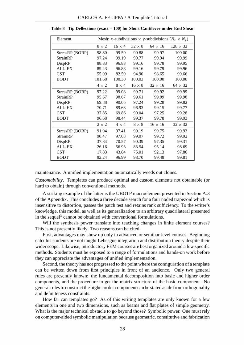
Table 8 Tip Deflections (exact = 100) for Short Cantilever under End Shear
Element Mesh: x-subdivisions × y-subdivisions (Nx × Ny)
8 × 2 16 × 4 32 × 8 64 × 16 128 × 32
StressRP (BORP) 98.80 99.59 99.88 99.97 100.00StrainRP 97.24 99.19 99.77 99.94 99.99DispRP 88.83 96.83 99.16 99.78 99.95ALL-EX 89.43 96.88 99.16 99.79 99.96CST 55.09 82.59 94.90 98.65 99.66BODT 101.68 100.30 100.03 100.00 100.00
4 × 2 8 × 4 16 × 8 32 × 16 64 × 32
StressRP (BORP) 97.22 99.08 99.71 99.92 99.99StrainRP 95.67 98.67 99.61 99.89 99.98DispRP 69.88 90.05 97.24 99.28 99.82ALL-EX 70.71 89.63 96.93 99.15 99.77CST 37.85 69.86 90.04 97.25 99.28BODT 96.68 98.44 99.37 99.78 99.93
2 × 2 4 × 4 8 × 8 16 × 16 32 × 32
StressRP (BORP) 91.94 97.41 99.19 99.75 99.93StrainRP 90.47 97.03 99.07 99.72 99.92DispRP 37.84 70.57 90.39 97.35 99.31ALL-EX 26.16 56.93 83.54 95.14 98.69CST 17.83 43.84 75.01 92.13 97.86BODT 92.24 96.99 98.70 99.48 99.81
maintenance. A unified implementation automatically weeds out clones.
Customability. Templates can produce optimal and custom elements not obtainable (orhard to obtain) through conventional methods.
A striking example of the latter is the UBOTP macroelement presented in Section A.3of the Appendix. This concludes a three decade search for a four noded trapezoid which isinsensitive to distortion, passes the patch test and retains rank sufficiency. To the writer’sknowledge, this model, as well as its generalization to an arbitrary quadrilateral presentedin the sequel3 cannot be obtained with conventional formulations.
Will the synthesis power translate into teaching changes in finite element courses?This is not presently likely. Two reasons can be cited.
First, advantages may show up only in advanced or seminar-level courses. Beginningcalculus students are not taught Lebesgue integration and distribution theory despite theirwider scope. Likewise, introductory FEM courses are best organized around a few specificmethods. Students must be exposed to a range of formulations and hands-on work beforethey can appreciate the advantages of unified implementation.
Second, the theory has not progressed to the point where the configuration of a templatecan be written down from first principles in front of an audience. Only two generalrules are presently known: the fundamental decomposition into basic and higher ordercomponents, and the procedure to get the matrix structure of the basic component. Nogeneral rules to construct the higher order component can be stated aside from orthogonalityand definiteness constraints.
How far can templates go? As of this writing templates are only known for a fewelements in one and two dimensions, such as beams and flat plates of simple geometry.What is the major technical obstacle to go beyond those? Symbolic power. One must relyon computer-aided symbolic manipulation because geometric, constitutive and fabrication
28

COMPUTATIONAL MECHANICS – THEORY AND PRACTICE
properties must be carried along as variables. This can lead, and does, to a combinatorialtarpit as elements become more complicated.
The good news is that computer algebra programs are gradually becoming more pow-erful, and are now routinely available on laptops and personal computers. Over the next5 years PCs are expected to migrate to 64-bit multiple-CPUs capable of addressing hun-dreds of GBs of memory at over 10GHz cycle speeds. As that happens the developmentof templates for 3D solid and shell elements in reasonable time will become possible.
Acknowledgements
Preparation of this paper has been supported by the National Science Foundation under Grant CMS–0219422, by the Finite Elements for Salinas contract with Sandia National Laboratories, and bya faculty fellowship from the Ministerio de Educacion y Cultura de Espana to visit the CentroInternacional de Metodos Numericos en Ingenerıa (CIMNE) in Barcelona from April to July 2002.
References
[1] M. J. Turner, R. W. Clough, H. C. Martin and L. J. Topp, Stiffness and deflection analysis ofcomplex structures, J. Aero. Sci., 23, 805–824 (1956).
[2] R. H. MacNeal, A theorem regarding the locking of tapered four noded membrane elements,Int. J. Numer. Meth. Engrg., 24, 1793–1799 (1987).
[3] C. A. Felippa, A 4-noded quadrilateral that sidesteps MacNeal’s theorem, in preparation.
[4] C. A. Felippa, A historical outline of matrix structural analysis: a play in three acts, Computers& Structures, 79, 1313–1324 (2001).
[5] J. H. Argyris and S. Kelsey, Energy Theorems and Structural Analysis, London, Butterworth(1960). Part I reprinted from Aircr. Engrg., 26, Oct-Nov 1954 and 27, April-May 1955.
[6] E. C. Pestel and F. A. Leckie, Matrix Methods in Elastomechanics, McGraw-Hill, New York,(1963).
[7] J. S. Przemieniecki, Theory of Matrix Structural Analysis, McGraw-Hill, New York (1968).Dover edition (1986).
[8] R. H. Gallaguer, A Correlation Study of Methods of Matrix Structural Analysis, Pergamon,Oxford (1964).
[9] R. F. Melosh, Bases for the derivation of matrices for the direct stiffness method, AIAA J., 1,1631–1637 (1963).
[10] M. J. Turner, The direct stiffness method of structural analysis, Structural and Materials PanelPaper, AGARD Meeting, Aachen, Germany (1959).
[11] M. J. Turner, E. H. Dill, H. C. Martin and R. J. Melosh, Large deflection analysis of complexstructures subjected to heating and external loads, J. Aero. Sci., 27, pp. 97-107 (1960).
[12] M. J. Turner, H. C. Martin and R. C. Weikel, Further development and applications of thestiffness method, in AGARDograph 72: Matrix Methods of Structural Analysis, ed. by B. M.Fraeijs de Veubeke, Pergamon Press, New York, 203–266 (1964).
[13] R. F. Melosh, Development of the stiffness method to define bounds on the elastic behavior ofstructures, Ph.D. Dissertation, University of Washington, Seattle (1962).
[14] B. M. Fraeijs de Veubeke, Upper and lower bounds in matrix structural analysis, in AGARDo-graph 72: Matrix Methods of Structural Analysis, ed. by B. M. Fraeijs de Veubeke, PergamonPress, New York, 174–265 (1964).
[15] R. W. Clough, The finite element method – a personal view of its original formulation, in FromFinite Elements to the Troll Platform – the Ivar Holand 70th Anniversary Volume, ed. by K.Bell, Tapir, Norway, 89–100 (1994).
[16] R. W. Clough, The finite element method in plane stress analysis, Proc. 2nd ASCE Conf. onElectronic Computation, Pittsburgh, Pa (1960).
[17] R. W. Clough, The finite element method in structural mechanics, in Stress Analysis, ed. byO. C. Zienkiewicz and G. S. Holister, Wiley, London, 85–119 (1965).
29

CARLOS A. FELIPPA / A Template Tutorial
[18] B. M. Fraeijs de Veubeke, Displacement and equilibrium models, in Stress Analysis, ed. by O.C. Zienkiewicz and G. Hollister, Wiley, London, 145–197, 1965; reprinted in Int. J. Numer.Meth. Engrg., 52, 287–342 (2001).
[19] O. C. Zienkiewicz and Y. K. Cheung, The Finite Element Method in Engineering Science,McGraw-Hill, London (1967).
[20] O. C. Zienkiewicz and Y. K. Cheung, Finite elements in the solution of field problems, TheEngineer, 507–510 (1965).
[21] B. M. Irons, Engineering application of numerical integration in stiffness methods, AIAA J.,4, pp. 2035–2037 (1966).
[22] B. M. Irons and J. Barlow, Comments on ‘matrices for the direct stiffness method’ by R. J.Melosh, AIAA J., 2, 403 (1964).
[23] G.P. Bazeley, Y. K. Cheung, B. M. Irons and O. C. Zienkiewicz, Triangular elements in platebending – conforming and nonconforming solutions, in Proc. 1st Conf. Matrix Meth. Struc.Mech., ed. by J. Przemieniecki et. al., AFFDL-TR-66-80, Air Force Institute of Technology,Dayton, Ohio, 547–576 (1966).
[24] J. Ergatoudis, B. M. Irons and O. C. Zienkiewicz, Curved, isoparametric, “quadrilateral”elements for finite element analysis, Int. J. Solids Struc., 4, 31–42 (1968).
[25] B. M. Irons and S. Ahmad, Techniques of Finite Elements, Ellis Horwood Ltd, Chichester, UK(1980).
[26] T. H. H. Pian, Derivation of element stiffness matrices by assumed stress distributions, AIAAJ., 2, 1333–1336 (1964).
[27] T. H. H. Pian, Element stiffness matrices for boundary compatibility and for prescribed bound-ary stresses, in Proc. 1st Conf. on Matrix Methods in Structural Mechanics, AFFDL-TR-66-80,Air Force Institute of Technology, Dayton, Ohio, 457–478 (1966).
[28] T. H. H. Pian and P. Tong, Basis of finite element methods for solid continua, Int. J. Numer.Meth. Engrg., 1, 3–29 (1969).
[29] T. H. H. Pian, Some notes on the early history of hybrid stress finite element method, Int. J.Numer. Meth. Engrg., 47, 419–425 (2000).
[30] L. R. Herrmann, Elasticity equations for nearly incompressible materials by a variationaltheorem, AIAA Journal, 3, 1896–1900 (1965).
[31] R. L. Taylor, K. S. Pister and L. R. Herrmann, A variational principle for incompressible andnearly incompressible orthotropic elasticity, Int. J. Solids Struc., 4, 875-883 (1968).
[32] G. Strang and G. Fix, An Analysis of the Finite Element Method. Prentice-Hall, (1973).[33] G. Strang, Variational crimes in the finite element method, in The Mathematical Foundations
of the Finite Element Method with Applications to Partial Differential Equations, ed. by A. K.Aziz, Academic Press, New York, 689–710 (1972).
[34] T. J. R. Hughes, The Finite Element Method: Linear Static and Dynamic Finite ElementAnalysis, Prentice Hall, Englewood Cliffs, N. J. (1987).
[35] K.-J. Bathe, Finite Element Procedures in Engineering Analysis, Prentice Hall, EnglewoodCliffs, N. J., 1982.
[36] S. N. Atluri, R. N. Gallagher and O. C. Zienkiewicz, (eds.), Hybrid and Mixed Finite ElementMethods, Wiley, New York (1983).
[37] R. H. MacNeal, Derivation of element stiffness matrices by assumed strain distribution, NuclearEngrg. Design, 70, 3–12 (1978)
[38] B. Szabo and I. Babuska, Finite Element Analysis Wiley, New York (1991).[39] R. H. MacNeal, The evolution of lower order plate and shell elements in MSC/NASTRAN, in
T. J. R. Hughes and E. Hinton (eds.), Finite Element Methods for Plate and Shell Structures,Vol. I: Element Technology, Pineridge Press, Swansea, U.K., 85–127 (1986).
[40] R. H. MacNeal, Finite Elements: Their Design and Performance, Marcel Dekker, New York(1994).
[41] P. G. Bergan, Finite elements based on energy orthogonal functions, Int. J. Numer. Meth.Engrg., 15, 1141–1555 (1980).
30

COMPUTATIONAL MECHANICS – THEORY AND PRACTICE
[42] P. G. Bergan and M. K. Nygard, Finite elements with increased freedom in choosing shapefunctions, Int. J. Numer. Meth. Engrg., 20, 643–664 (1984).
[43] D. P. Flanagan and T. Belytschko, A uniform strain hexahedron and quadrilateral with orthog-onal hourglass control, Int. J. Numer. Meth. Engrg., 17, 679–706 (1981).
[44] K.-J. Bathe and E. N. Dvorkin, A four-node plate bending element based on Mindlin-Reissnerplate theory and a mixed interpolation, Int. J. Numer. Meth. Engrg., 21, 367–383 (1985).
[45] H. C. Huang and E. Hinton, A new nine node degenerated shell element with enhancedmembrane and shear interpolation, Int. J. Numer. Meth. Engrg., 22, 73–92 (1986).
[46] K. C. Park, G. M. Stanley, A curved C0 shell element based on assumed natural-coordinatestrains, J. Appl. Mech., 53, 278–290 (1986).
[47] G. M. Stanley, K. C. Park and T. J. R. Hughes, Continuum based resultant shell elements, inT. J. R. Hughes and E. Hinton (eds.), Finite Element Methods for Plate and Shell Structures,Vol. I: Element Technology, Pineridge Press, Swansea, U.K., 1–45 (1986)
[48] T. H. H. Pian and K. Sumihara, Rational approach for assumed stress finite elements, Int. J.Numer. Meth. Engrg., 20, 1685–1695 (1984).
[49] T. H. H. Pian and P. Tong, Relations between incompatible displacement model and hybridstress model, Int. J. Numer. Meth. Engrg., 22, 173-181 (1986).
[50] E. F. Punch and S. N. Atluri, Development and testing of stable, invariant, isoparametriccurvilinear 2- and 3D hybrid stress elements, Comp. Meths. Appl. Mech. Engrg., 47, 331–356(1984).
[51] C. Militello and C. A. Felippa, The First ANDES Elements: 9-DOF Plate Bending Triangles,Comp. Meths. Appl. Mech. Engrg., 93, 217–246 (1991).
[52] C. A. Felippa and C. Militello, Membrane triangles with corner drilling freedoms: II. TheANDES element, Finite Elements Anal. Des., 12, 189–201 (1992).
[53] J. C. Simo and T. J. R. Hughes, On the variational foundations of assumed strain methods, J.Appl. Mech., 53, 51–54 (1986).
[54] J. C. Simo and M. S. Rifai, A class of mixed assumed strain methods and the method ofincompatible modes, Int. J. Numer. Meth. Engrg., 29, 1595–1638 (1990).
[55] C. A. Felippa and C. Militello, Developments in variational methods for high performance plateand shell elements, in Analytical and Computational Models for Shells, CED Vol. 3, Eds. A. K.Noor, T. Belytschko and J. C. Simo, The American Society of Mechanical Engineers, ASME,New York, 191–216 (1989).
[56] P. G. Bergan and L. Hanssen, A New Approach for Deriving ‘Good’ Finite Elements, inThe Mathematics of Finite Elements and Applications – Volume II, ed. by J. R. Whiteman,Academic Press, London, 483–497, (1975).
[57] L. Hanssen, P. G. Bergan and T. J. Syversten, Stiffness derivation based on element convergencerequirements, in The Mathematics of Finite Elements and Applications – Volume III, ed. by J.R. Whiteman, Academic Press, London, 83–96, (1979).
[58] P. G. Bergan and C. A. Felippa, A triangular membrane element with rotational degrees offreedom, Comp. Meths. Appl. Mech. Engrg., 50, 25–69 (1985).
[59] B. M. Fraeijs de Veubeke, Diffusive equilibrium models, in M. Geradin (ed.), B. M. Fraeijsde Veubeke Memorial Volume of Selected Papers, Sitthoff & Noordhoff, Alphen aan den Rijn,The Netherlands, 569–628 (1980).
[60] P. G. Bergan and C. A. Felippa, Efficient implementation of a triangular membrane elementwith drilling freedoms, in T. J. R. Hughes and E. Hinton (eds.), Finite Element Methodsfor Plate and Shell Structures, Vol. I: Element Technology, Pineridge Press, Swansea, U.K.,128–152 (1986).
[61] M. K. Nygard, The Free Formulation for nonlinear finite elements with applications to shells,Ph. D. Dissertation, Division of Structural Mechanics, NTH, Trondheim, Norway (1986).
[62] C. A. Felippa and P. G. Bergan, A triangular plate bending element based on an energy-orthogonal free formulation, Comp. Meths. Appl. Mech. Engrg., 61, 129–160 (1987).
31

CARLOS A. FELIPPA / A Template Tutorial
[63] C. A. Felippa, Parametrized multifield variational principles in elasticity: II. Hybrid functionalsand the free formulation, Comm. Appl. Numer. Meth., 5, 79–88 (1989).
[64] C. A. Felippa, The extended free formulation of finite elements in linear elasticity, J. Appl.Mech., 56, 609–616 (1989).
[65] G. Skeie, The Free Formulation: linear theory and extensions with applications to tetrahedralelements with rotational freedoms, Ph. D. Dissertation, Division of Structural Mechanics,NTH, Trondheim, Norway (1991).
[66] C. A. Felippa and R. W. Clough, The finite element method in solid mechanics, in NumericalSolution of Field Problems in Continuum Physics, ed. by G. Birkhoff and R. S. Varga, SIAM–AMS Proceedings II, American Mathematical Society, Providence, R.I., 210–252 (1969).
[67] I. C. Taig and R. I. Kerr, Some problems in the discrete element representation of aircraftstructures, in Matrix Methods of Structural Analysis, ed. by B. M. Fraeijs de Veubeke,Pergamon Press, London (1964).
[68] E. L. Wilson, R. L. Taylor, W. P. Doherty and J. Ghaboussi, Incompatible displacement models,in Numerical and Computer Models in Structural Mechanics, ed. by S. J. Fenves, N. Perrone,A. R. Robinson and W. C. Schnobrich, Academic Press, New York, 43–57 (1973).
[69] R. L. Taylor, E. L. Wilson and P. J. Beresford, A nonconforming element for stress analysis,Int. J. Numer. Meth. Engrg., 10, 1211–1219 (1976).
[70] T. Belytschko, W. K. Liu and B. E. Engelmann, The gamma elements and related developments,in T. J. R. Hughes and E. Hinton (eds.), Finite Element Methods for Plate and Shell Structures,Vol. I: Element Technology, Pineridge Press, Swansea, U.K., 316–347 (1986).
[71] R. H. MacNeal, A simple quadrilateral shell element, Computers & Structures, 8, 175–183(1978).
[72] N. Lautersztajn-S and A. Samuelsson, Further discussion on four-node isoparametric elementsin plane bending, Int. J. Numer. Meth. Engrg., 47, 129–140 (2000).
[73] C. A. Felippa, A survey of parametrized variational principles and applications to computa-tional mechanics, Comp. Meths. Appl. Mech. Engrg., 113, 109–139 (1994).
[74] C. A. Felippa, B. Haugen and C. Militello, From the individual element test to finite elementtemplates: evolution of the patch test, Int. J. Numer. Meth. Engrg., 38, 199–222 (1995).
[75] C. A. Felippa, Parametrized unification of matrix structural analysis: classical formulation andd-connected mixed elements, Finite Elements Anal. Des., 21, 45–74 (1995).
[76] C. A. Felippa, Recent developments in parametrized variational principles for mechanics,Comput. Mech., 18, 159–174, 1996.
[77] C. A. Felippa and C. Militello, Construction of optimal 3-node plate bending elements bytemplates, Comput. Mech., 24, 1–13 (1999).
[78] C. A. Felippa, Recent developments in basic finite element technologies, in ComputationalMechanics in Structural Engineering-Recent Developments, ed. by F.Y. Cheng and Y. Gu,Elsevier, Amsterdam, 141–156, 1999.
[79] C. A. Felippa, Recent advances in finite element templates, in Computational Mechanics forthe Twenty-First Century, ed. by B.J.V. Topping, Saxe-Coburn Pub., Edinburgh, 71–98, 2000.
[80] C. Militello and C. A. Felippa, The individual element patch revisited, in The Finite ElementMethod in the 1990’s — a book dedicated to O. C. Zienkiewicz, ed. by E. Onate, J. Periauxand A. Samuelsson, CIMNE, Barcelona and Springer-Verlag, Berlin, 554–564 (1991).
[81] C. A. Felippa, A study of optimal membrane triangles with drilling freedoms, Comp. Meths.Appl. Mech. Engrg., 192, 2125–2168 (2003).
[82] C. A. Felippa, Customizing the mass and geometric stiffness of plane thin beam elements byFourier methods, Engrg. Comput., 18, 286–303 (2001).
[83] C. A. Felippa, Customizing high performance elements by Fourier methods, Trends in Com-putational Mechanics, ed. by W. A. Wall, K.-U. Bleitzinger and K. Schweizerhof, CIMNE,Barcelona, Spain, 283-296 (2001).
[84] W. P. Doherty, E. L. Wilson and R. L. Taylor, Stress analysis of axisymmetric solids utilizinghigher order quadrilateral finite elements, SESM Report 69-3, Department of Civil Engineer-ing, University of California, Berkeley (1969).
32

COMPUTATIONAL MECHANICS – THEORY AND PRACTICE
[85] O. C. Zienkiewicz, R. L. Taylor and J. M. Too, Reduced integration technique in generalanalysis of plates and shells, Int. J. Numer. Meth. Engrg., 3, 275–290 (1971).
[86] S. F. Pawsey and R. W. Clough, Improved numerical integration of thick shell finite elements,Int. J. Numer. Meth. Engrg., 3, 545–586 (1971).
[87] K. Kavanagh and S. W. Key, A note on selective and reduced integration techniques in thefinite element method, Int. J. Numer. Meth. Engrg., 4, 148–150 (1972).
[88] T. J. R. Hughes, Generalization of selective integration procedures to anisotropic and nonlinearmedia, Int. J. Numer. Meth. Engrg., 15, 1413–148 (1980).
[89] T. J. R. Hughes and D. S. Malkus, Mixed finite element methods – reduced and selectiveintegration techniques: a unification of concepts, Comp. Meths. Appl. Mech. Engrg., bf 15,63–81 (1978).
[90] T. J. R. Hughes and D. S. Malkus, A general penalty mixed equivalence theorem for anisotropic,incompressible finite elements, in Hybrids and Mixed Finite Element Methods, ed. by S. N.Atluri, R. H. Gallagher and O. C. Zienkiewicz, Wiley, London (1983).
[91] K. Alvin, H. M. de la Fuente, B. Haugen and C. A. Felippa, Membrane triangles with cornerdrilling freedoms: I. The EFF element, Finite Elements Anal. Des., 12, 163–187 (1992).
[92] C. A. Felippa and S. Alexander, Membrane triangles with corner drilling freedoms: III. Im-plementation and performance evaluation, Finite Elements Anal. Des., 12, 203–239 (1992).
[93] D. J. Allman, Evaluation of the constant strain triangle with drilling rotations, Int. J. Numer.Meth. Engrg., 26, 2645–2655 (1988).
[94] C. A. Felippa, Refined finite element analysis of linear and nonlinear two-dimensional struc-tures, Ph.D. Dissertation, Department of Civil Engineering, University of California at Berke-ley, Berkeley, CA (1966).
[95] C. A. Felippa and K. C. Park, Fitting strains and displacements by minimizing dislocationenergy, Proceedings of the Sixth International Conference on Computational Structures Tech-nology, Prague, Czech Republic, 49–51 (2002). Complete text in CDROM.
[96] C. A. Felippa and K. C. Park, The construction of free-free flexibility matrices for multilevelstructural analysis, Comp. Meths. Appl. Mech. Engrg., 191, 2111-2140 (2002).
[97] R. H. MacNeal and R. L. Harder, A proposed standard set of problems to test finite elementaccuracy, Finite Elements Anal. Des., 1, 3–20 (1985).
[98] C. C. Wu and Y. K. Cheung, On optimization approaches of hybrid stress elements, FiniteElements Anal. Des., 21, 111–128 (1995).
33

CARLOS A. FELIPPA / A Template Tutorial
Appendix A. MORE GENERAL PANEL GEOMETRIES
The template framework of four noded membrane elements can be extended to moregeneral geometries, at the cost of increased complexity in symbolic computations. As anaperitif for the sequel3 this appendix present templates for parallelogram and trapezoidalgeometries.
The first-generation (pre-1962) direct elasticity methods recalled in Sections 4–5 donot work properly beyond the parallelogram. The resulting “node collocation” elementsfail the patch test and thus cannot fit in the template framework.
Variational methods are required to get stress-assumed and strain-assumed elements that work. Forstress elements the Hellinger-Reissner (HR) princi-ple is used. For strain elements, a strain-fit method95
in conjunction with de Veubeke’s strain-displacementmixed functional is used.
A.1 Parallelogram (Swept) Panel
The geometry of the parallelogram panel shown inFigure 17 is defined by the dimensions a, b and the ske-wangle ω, positive counterclockwise. The templateagain has the configuration (31) displayed in Figure 6.
1 2
34
a
b = a/γ x
x
yωω
ω
ω
y
Constant thickness hand elasticity matrix E
Figure 17. The 4-node swept panel.
With s = tan ω the matrices to be adjusted are
W =[ 1
a 0
− sb
1b
],
Hc = 1
2ab
[ −b 0 b 0 b 0 −b 00 −a − bs 0 −a + bs 0 a + bs 0 a − bs
−a − bs −b −a + bs b a + bs b a − bs −b
],
(63)
The higher order projector Hh is exactly as in (32), whereas R depends on the formu-lation, as explained below. For future use the compliance and elasticity along the mediandirection yω (see Figure 17) are denoted by
Cω22 = C22 cos4 ω − 2C23 cos3 ω sin ω + (2C12+C33) cos2 ω sin2 ω − 2C13 cos ω sin3 ω
+ C11 sin4 ω = C22 − 2C23s + (2C12 + C33)s2 − 2C13s3 + C11s4
(1 + s2)2,
Eω22 = E22 cos4 ω − 4E23 cos3 ω sin ω + (2E12+4E33) cos2 ω sin2 ω − 4E13 cos ω sin3 ω
+ E11 sin4 ω = E22 − 4E23s + (2E12 + 4E33)s2 − 4E13s3 + E11s4
(1 + s2)2.
(64)
Stress element. A 5-parameter stress element StressPP can be constructed either directly,as done by Gallagher8 or by the HR principle, starting from the energy-orthogonal stressfield
[σxx
σyy
σxy
]=
[ 1 0 0 y/b sin2 ω xω
0 1 0 0 cos2 ω xω
0 0 1 0 − sin ω cos ω xω
]
µ1
µ2
µ3
µ4
µ5
, (65)
34
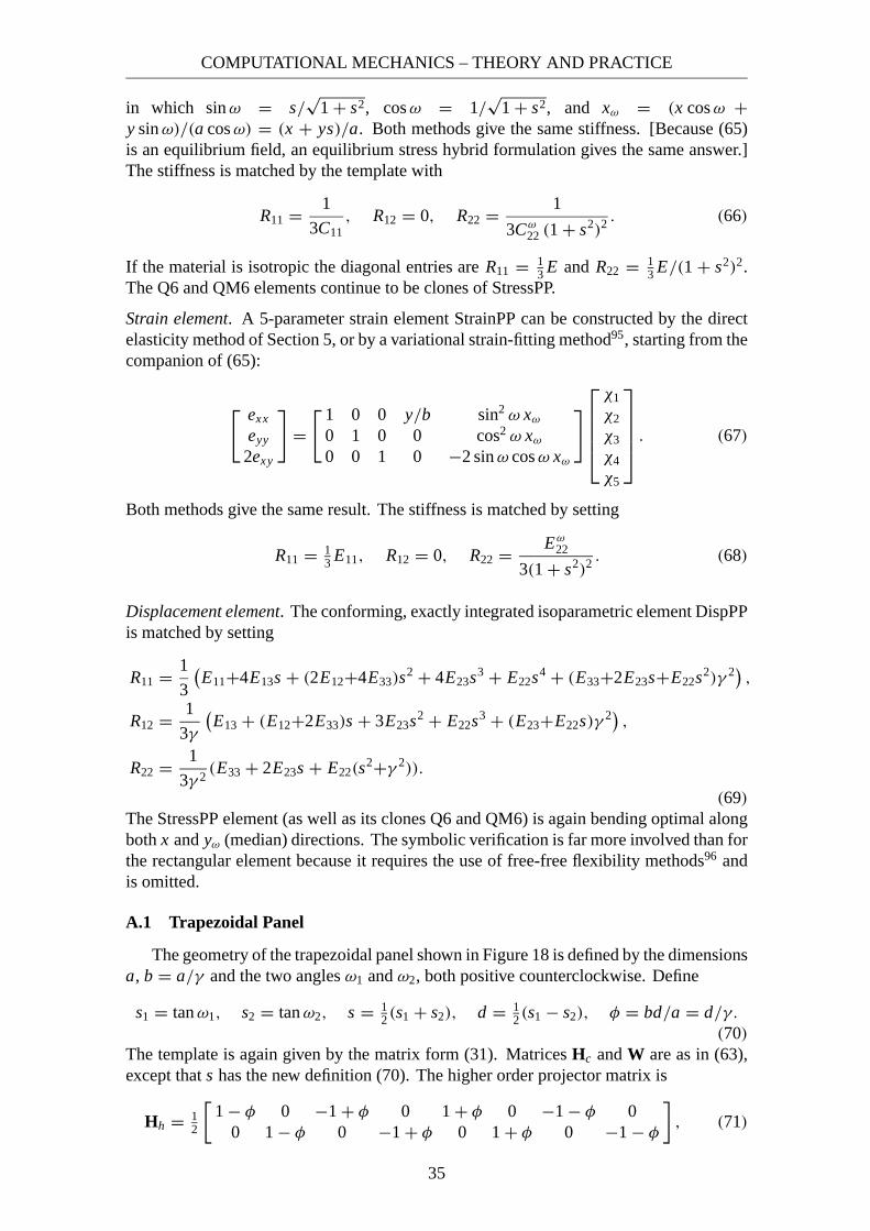
COMPUTATIONAL MECHANICS – THEORY AND PRACTICE
in which sin ω = s/√
1 + s2, cos ω = 1/√
1 + s2, and xω = (x cos ω +y sin ω)/(a cos ω) = (x + ys)/a. Both methods give the same stiffness. [Because (65)is an equilibrium field, an equilibrium stress hybrid formulation gives the same answer.]The stiffness is matched by the template with
R11 = 1
3C11, R12 = 0, R22 = 1
3Cω22 (1 + s2)2 . (66)
If the material is isotropic the diagonal entries are R11 = 13 E and R22 = 1
3 E/(1 + s2)2.The Q6 and QM6 elements continue to be clones of StressPP.
Strain element. A 5-parameter strain element StrainPP can be constructed by the directelasticity method of Section 5, or by a variational strain-fitting method95, starting from thecompanion of (65):
[ exx
eyy
2exy
]=
[ 1 0 0 y/b sin2 ω xω
0 1 0 0 cos2 ω xω
0 0 1 0 −2 sin ω cos ω xω
]
χ1
χ2
χ3
χ4
χ5
. (67)
Both methods give the same result. The stiffness is matched by setting
R11 = 13 E11, R12 = 0, R22 = Eω
22
3(1 + s2)2 . (68)
Displacement element. The conforming, exactly integrated isoparametric element DispPPis matched by setting
R11 = 1
3
(E11+4E13s + (2E12+4E33)s
2 + 4E23s3 + E22s4 + (E33+2E23s+E22s2)γ 2),
R12 = 1
3γ
(E13 + (E12+2E33)s + 3E23s2 + E22s3 + (E23+E22s)γ 2
),
R22 = 1
3γ 2(E33 + 2E23s + E22(s
2+γ 2)).
(69)
The StressPP element (as well as its clones Q6 and QM6) is again bending optimal alongboth x and yω (median) directions. The symbolic verification is far more involved than forthe rectangular element because it requires the use of free-free flexibility methods96 andis omitted.
A.1 Trapezoidal Panel
The geometry of the trapezoidal panel shown in Figure 18 is defined by the dimensionsa, b = a/γ and the two angles ω1 and ω2, both positive counterclockwise. Define
s1 = tan ω1, s2 = tan ω2, s = 12 (s1 + s2), d = 1
2 (s1 − s2), φ = bd/a = d/γ.
(70)
The template is again given by the matrix form (31). Matrices Hc and W are as in (63),except that s has the new definition (70). The higher order projector matrix is
Hh = 12
[1 − φ 0 −1 + φ 0 1 + φ 0 −1 − φ 0
0 1 − φ 0 −1 + φ 0 1 + φ 0 −1 − φ
], (71)
35
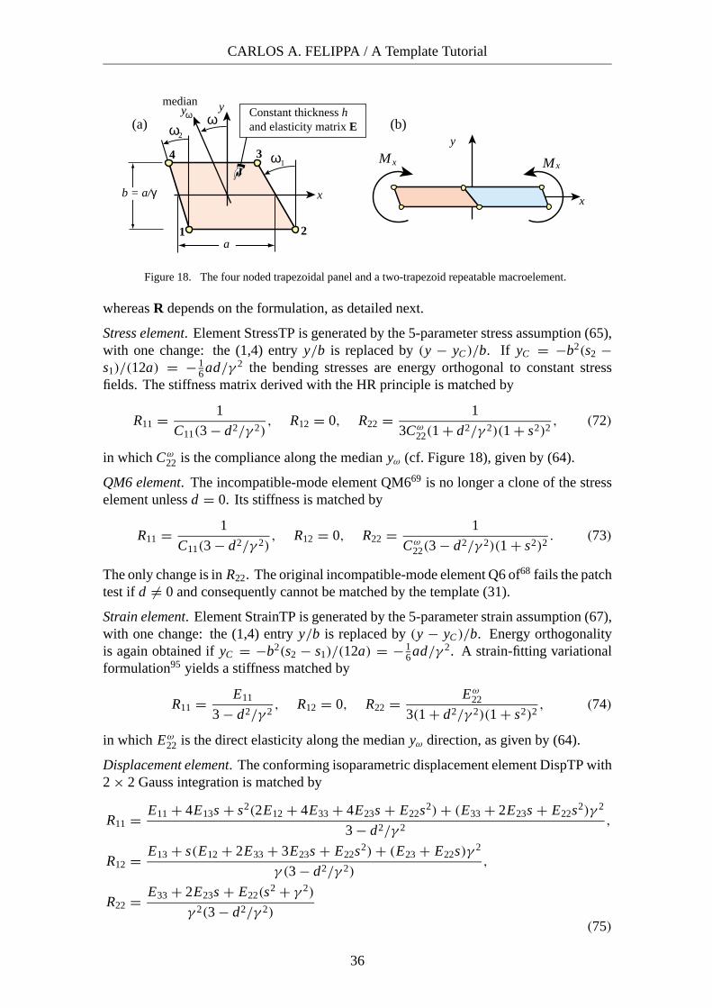
CARLOS A. FELIPPA / A Template Tutorial
1 2
34
b = a/γ x
y
M Mx x
x
y
ω1
ω2
ω
a
(a) (b)ωy
medianConstant thickness hand elasticity matrix E
Figure 18. The four noded trapezoidal panel and a two-trapezoid repeatable macroelement.
whereas R depends on the formulation, as detailed next.
Stress element. Element StressTP is generated by the 5-parameter stress assumption (65),with one change: the (1,4) entry y/b is replaced by (y − yC)/b. If yC = −b2(s2 −s1)/(12a) = − 1
6 ad/γ 2 the bending stresses are energy orthogonal to constant stressfields. The stiffness matrix derived with the HR principle is matched by
R11 = 1
C11(3 − d2/γ 2), R12 = 0, R22 = 1
3Cω22(1 + d2/γ 2)(1 + s2)2
, (72)
in which Cω22 is the compliance along the median yω (cf. Figure 18), given by (64).
QM6 element. The incompatible-mode element QM669 is no longer a clone of the stresselement unless d = 0. Its stiffness is matched by
R11 = 1
C11(3 − d2/γ 2), R12 = 0, R22 = 1
Cω22(3 − d2/γ 2)(1 + s2)2
. (73)
The only change is in R22. The original incompatible-mode element Q6 of68 fails the patchtest if d �= 0 and consequently cannot be matched by the template (31).
Strain element. Element StrainTP is generated by the 5-parameter strain assumption (67),with one change: the (1,4) entry y/b is replaced by (y − yC)/b. Energy orthogonalityis again obtained if yC = −b2(s2 − s1)/(12a) = − 1
6 ad/γ 2. A strain-fitting variationalformulation95 yields a stiffness matched by
R11 = E11
3 − d2/γ 2, R12 = 0, R22 = Eω
22
3(1 + d2/γ 2)(1 + s2)2, (74)
in which Eω22 is the direct elasticity along the median yω direction, as given by (64).
Displacement element. The conforming isoparametric displacement element DispTP with2 × 2 Gauss integration is matched by
R11 = E11 + 4E13s + s2(2E12 + 4E33 + 4E23s + E22s2) + (E33 + 2E23s + E22s2)γ 2
3 − d2/γ 2,
R12 = E13 + s(E12 + 2E33 + 3E23s + E22s2) + (E23 + E22s)γ 2
γ (3 − d2/γ 2),
R22 = E33 + 2E23s + E22(s2 + γ 2)
γ 2(3 − d2/γ 2)(75)
36

COMPUTATIONAL MECHANICS – THEORY AND PRACTICE
A.2 A Unidirectional-Bending-Optimal Trapezoidal Panel
Element StressTP is x-bending optimal as an individual element, but far from it as arepeating macroelement. Consider the configuration of Figure 18(b): two mirror-imagetrapezoidal elements are glued to form a parallelogram macroelement. The macroelementshape is that of a swept panel, and is obviously repeatable along x .
If a >> b and s1 �= s2 the StressTP-fabricated macroelement rapidly becomes overstiffand overflexible in x- and y-bending, respectively. For example if a/b = γ = 8, s1 = 0,s2 = 1/2 and isotropic material with ν = 1/4 the bending ratios are rx = 11.97 andry = 0.1414. For the anisotropic elasticity matrix (61), rx = 6.93 and ry = 0.0792. Ifan elongated macroelement is supposed to model unidirectional x-bending correctly, theoverstiffness caused by s1 �= s2 is called distortion locking. This phenomenon has beenwidely studied since the MacNeal-Harder test suite gained popularity.97
It is possible to construct a trapezoidal panel that is exact in unidirectional x bendingwhen configured to form a repeatable macroelement as in Figure 18(b), for any aspect ratioγ as well as arbitrary side slopes s1 and s2. This template instance will be called UBOTP.A compact expression is obtained by taking the R matrix of StressTP, generated by (72)and modifying the (2,1) entry of W:
W = 1/a 0
−(C11(3γ 2 − ds) + C13
)(s − d) − C12d
C11(3γ 2 − d2)b1/b
(76)
It would be equally possible tokeep W of (63) and adjust the en-tries of R. However, the correc-tion (76) suggests how this optimal-ity result is extendible to arbitraryquadrilaterals.3 It is not difficult toprove that WT RW for UBOTP ispositive definite as long as the trape-zoid is convex. [Not only that: itscondition number is bounded, whichis another way of saying that the inf-sup — also called LBB condition —is verified.] Consequently the ele-ment stiffness is nonnegative, andhas the correct rank.
Figure 19 presents results fora widely used mesh distortion test,which involves one macroelement ofthe type discussed. Results for sixelement types: UBOTP, StressTP,StrainTP, DispTP, Q6 and QM6 areshown. The percentage of the cor-rect answer is of course 100/rx .
���
2a = 10
b =2 M /bx
M /bx
E = 1500, ν = 1/4, h = 1
Perc
enta
ge o
f ex
act a
nsw
er
Distortion parameter 2e/b
UBOTP
Q6
1 2 3 4 5
20
40
60
80
100
StressTP
StrainTP
DispTP
QM6
e
Figure 19. A well known distortion benchmark test.Dashed lines mark elements that fail thepatch test (only Q6 in this particular set).
Of these six models only Q6 fails the patch test, but otherwise works better than allothers but UBOTP. StressTP, StrainTP and QM6 give similar results, as can be expected,whereas DispTP is way overstiff even for zero distortion. UBOTP gives the correct resultfor all distortion parameters from 0 through 5, since rx ≡ 1. If the aspect ratio of the
37

CARLOS A. FELIPPA / A Template Tutorial
cantilever is changed to, say 2a/b = 10, the differences between elements become moredramatic.
For distortion performance results on other elements such as Pian-Sumihara and En-hanced Assumed Strain, see Lautersztajn and Samuelsson.72 A penalty-augmented modi-fication of the Pian-Sumihara quadrilateral constructed by Wu and Cheung98 that achievesdistortion insensitivity at the cost of rank deficiency (and hence fails the inf-sup condition)is discussed in the sequel.3
At first sight the existence of UBOTP contradicts a theorem by MacNeal,2 which saysthat four noded quadrilaterals cannot simultaneously pass the patch test and be insensitiveto distortion. The escape hatch is that y-bending optimality (along the skew angulardirection ω1 of the macroelement) is not attempted. If one tries imposing rx = ry = 1, thesolutions for {R11, R12, R22} become complex if γ >> 1 as soon as d deviates slightlyfrom zero.
38