A test-rig for the Inline-CVT Report of my internship at UC Davis.

By Niels Scheffer

july 2005

Advisors: - UC Davis: Prof Dr A.A. Frank, PhD, PhD - TU Eindhoven: Dr. B. Veenhuizen.

Department of Mechanical and Aeronautical Engineering, Hybrid Electric Vehicle Center, University of California, Davis, U.S.A. Department of Mechanical Engineering, Power Trains, Technical University of Eindhoven, the Netherlands.

Introduction Following is a report of the work I have been doing the past few months at the HEV Center of UC Davis. I have been working here for my internship as a part of the program for my master in Mechanical Engineering. At the UC, I have been working on the development of a test-rig for a new kind of continuous variable transmission, the Inline-CVT. I have been doing this internship together with Guus Arts, another student of the TU of Eindhoven. In this report, I will mention some of his work, and use it as a reference sometimes. The final report that remains here in Davis, will be a combination of both our reports. The Department of Mechanical and Aeronautical Engineering of the University of California Davis, is currently developing a new kind of transmission. This research is part of the Hybrid Electric Vehicle program. The basic idea and concepts behind this transmission, is from Prof. Dr. A.A. Frank, also head of the HEV Center. This transmission has to be tested and therefore we had to build this test-rig. The making of this test-rig is dealt with in this report, discussing the choices we had to make, the mistakes we made, the drawbacks and the progress.

2

Table of contents Introduction 2 Table of contents 3 1. In short

1.1 Basic idea 4 1.2 Set-up 4

2. Shafts 2.1 Input shaft 5 2.2 Output shaft 6 2.3 The key 7 3. Hydraulic system 3.1 System outline 8 3.2 Determining parameters 8 3.3 Choosing pulleys 9 3.4 Choosing the belt 10 3.5 Results 10 3.6 Mounting plate 3.6.1 Production 11 3.6.2 Current status 13 4. Wiring 4.1 Strain gauge 14 4.2 LVDT 14 4.3 Electromotor 15 5. AMC 5.1 AMC 16 5.2 PXI 16 6. LabView 6.1 LabView 21 6.2 Operating 24 7. Power source 7.1 Power source 27 8. Mounting sensors 8.1 Strain gauge 28 8.2 LVDT 28 9. Noise 9.1 General 33 9.2 Protecting against noise 33 9.3 Noise source 33 9.4 Recommendations 33 Conclusion 36 Sources 37

3

1. In short 1.1 Basic idea The Inline-CVT is a new kind of continuous variable transmission based upon the pulley and belt system, also known as the ‘van Doorne’ principle. The used belt is the GCI chain, a new kind of chain developed by Gear Chain Industrial BV. This chain has special designed links and is a totally new design, with a higher efficiency then the ‘normal’ chain of VDT. The Inline however, contains two belt and pulley sets, in one transmission. It is basically two CVTs in series. The output shaft is then again inline with the input shaft. Of course, there is more to it, but this is just the basic idea. Our original assignment was to measure and calculate the efficiency of the Inline. But when we arrived here in Davis, it became clear that we first had to built a test-rig, complete with all the sensors and controls, before we could perform any tests on the Inline. We started with a dynamometer (not working), an electromotor for the input power and torque (not working) and a stand where the Inline was mounted in. Further there were remains of previous tests, so lots of wires and sensors everywhere. We had to clean up the lab, finish the stand, order some shafts, make a hydraulic system, mount and test all the sensors, install a control toolbox, learn how to get the dynamometer and the electromotor working again, learn how to use the control toolbox, and get everything working. 1.2 The set up To make sure it is clear what I am talking about, hereby a short description of the set-up. An electromotor, the AC150, propels the Inline-CVT through a flexible coupling. The outgoing shaft of the Inline is connected with a shaft with two u-joints to a dynamometer. The dynamometer and the AC150 are both controlled by the Superflow computer, a remote desktop outside the lab for safety reasons. The Inline-CVT has three Hall sensors, two pressure sensors, a thermo sensor, a LVDT (ratio-sensor) and the hydraulic system all controlled by the LabView computer, a control toolbox inside the lab.

4

2. Shafts Between the electromotor, the inline-cvt and the brake, connections have to be made. As a connection, on the input side of the inline-cvt, there can be a fixed, rigid shaft. On one side it goes into a tapered end, and on the other side it has a spline. The output shaft is more complicated, because some flexibility is needed. 2.1 Input shaft The input shaft is a rigid shaft, because it will slide into a flexible coupling on one side, to deal with vibrations. The output side of the electromotor and the input side of the inline-cvt are mounted onto the sides of a rigid steel box, after which they have been carefully aligned. Therefore, there is only need for a flexible coupling to compensate for vibrations. This flexible coupling is mounted onto to outgoing shaft of the electromotor, and has got a taper connection on the other side. On this taperfit hole, the shaft will be fixed, with external splines, going into the internal ones in the inline-cvt. These splines are of a standard size, namely DIN 5480. The length of this shaft has been chosen extra long, because it is always possible to make it shorter, and cut to fit.The taper end of the shaft will be made in our own machineshop. The exact length of the shaft is determined when the complete set-up is fixed into place.

Figure 1 : Input shaft final sizes

Figure 2: Input shaft and flexible coupling.

5

2.2 Output shaft The output shaft has to compensate for a height difference, and also correct any alignment faults. Because there is no other rigid connection between the inline-cvt and the brake then the floor they are mounted on, making a good alignment is difficult. It should be of no surprise that there are horizontal and vertical orientation differences. That is why the connecting axis is chosen to exist out of two universal joints welded together, to make a very short, but extremely flexible shaft. On the side of the inline-cvt a short shaft is made with again the external splines on one side, but this time a key shaft on the other side. To this key shaft a flange will be fitted with the holes in it on which the u-joints can be bolted. On the side of the brake a similar configuration will be mounted. Some pictures and drawings to make things more clearly:

Figure 3: Short shaft between CVT and U-joint shaft.

Figure 4: Output shaft

6

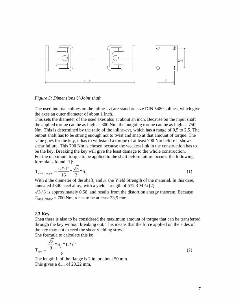
Figure 5: Dimensions U-Joint shaft. The used internal splines on the inline-cvt are standard size DIN 5480 splines, which give the axes an outer diameter of about 1 inch. This sets the diameter of the used axes also at about an inch. Because on the input shaft the applied torque can be as high as 300 Nm, the outgoing torque can be as high as 750 Nm. This is determined by the ratio of the inline-cvt, which has a range of 0,5 to 2,5. The output shaft has to be strong enough not to twist and snap at that amount of torque. The same goes for the key, it has to withstand a torque of at least 700 Nm before it shows shear failure. This 700 Nm is chosen because the weakest link in the construction has to be the key. Breaking the key will give the least damage to the whole construction. For the maximum torque to be applied to the shaft before failure occurs, the following formula is found [1]:

y

3

torque_shaft S*33*

16d*T π

= (1)

With d the diameter of the shaft, and Sy the Yield Strength of the material. In this case, annealed 4340 steel alloy, with a yield strength of 572,3 MPa [2]

3/3 is approximately 0.58, and results from the distortion energy theorem. Because Tshaft_torque = 700 Nm, d has to be at least 23,5 mm. 2.3 Key Then there is also to be considered the maximum amount of torque that can be transferred through the key without breaking out. This means that the force applied on the sides of the key may not exceed the shear yielding stress. The formula to calculate this is:

8

d*L*S*33

T

2y

key = (2)

The length L of the flange is 2 in, or about 50 mm. This gives a dmin of 20.22 mm.

7

By taking the diameter of the shaft 1 in (25.4 mm), it’s easy to manufacture, because of the standard size, and it meets the requirements as well. In general, the key is square and the height is about a fourth of the diameter of the axle, so the key will be ¼ inch high and 2 inch long.

8

3. Hydraulic system 3.1 System outline Two pumps provide the main oil pressure for the system. These pumps are powered by electromotors. Unfortunately, the speed ratio of the electromotors doesn’t match the needs of the input shaft of the hydraulic pumps. This can be solved in two different manners. One is to buy other electromotors. This seems to be the easiest solution, but electromotors that provide the right torque at the right rpm, are hard to get, and are also higher in price. The other option is to install a reduction gear. The reduction ratio has to be at least 2:1. To achieve this reduction, there are many possibilities. One of the first solutions was a gearbox, existing of a planetary set, which could achieve a 3:1 ratio, with the shafts of the motor and pump positioned inline. The gearboxes are custom-made, by Parker. [1] An quotation given by a supplier of Parker Gears, [2], showed prices that are too high to gain an economical advantage over buying other electromotors. Another solution is working with gears and sprockets. The motor and pump are both mounted onto a mounting plate, with their shafts parallel to each other. On the motorshaft a pulley or sprocket with half the diameter of the one on the pump is fitted. Between these sprockets or pulleys a belt of some type is fitted, thus providing a 2:1 ratio. The usual supplier of UC Davis is W.M. Berg [3]. They offer various types of belts and sprockets. 3.2 Determining parameters Before choosing a solution, the parameters must be known. The electromotor [4] will have a maximum of 5,000 rpm and has an output shaft diameter of 3/8”. The torque that the electromotor will deliver will be 10 Nm (7.4 lbf ft) max. The input shaft on the hydraulic pump is 7/16”. Because W.M. Berg doesn’t deliver any pulleys nor sprockets with a bore of 7/16”, pulleys and sprockets with a 3/8” bore were considered to be the best option, which will have to be overbored to fit. The spacing between the pump and the motor has to be at least 4”, because otherwise the motor and the pump cannot be alongside each other. While the input-pulley will be half the diameter of the output-pulley, they cannot be fit too close to each other either, because the angle at which the belt hits the smallest pulley will be too big and that will cause the belt to wear out very quick. Such a set-up also can be the cause of slip and reduced capability of transferring force. That is why the distance between the outer perimeters of the pulley is chosen to be at least one times the diameter of the largest pulley. Because the diameter of the largest pulley is twice the diameter of the smallest pulley, the total spacing becomes 7 times the radius of the smallest pulley. With the spacing being 4”, this gives a wanted diameter of the pulleys of (4/7)*2 = 1,2” for the input (d1) and 2,4” for the output (d2). The maximum operating load on the belt will then become approximately 150 lbs. That is derived from the 10 Nm of torque at a radius of 0,6” (15,24 mm). Which gives a force at the belt of Fload = 10 [Nm] / 15,24*10-3 [m] = 656 [N], equal to (3)

9

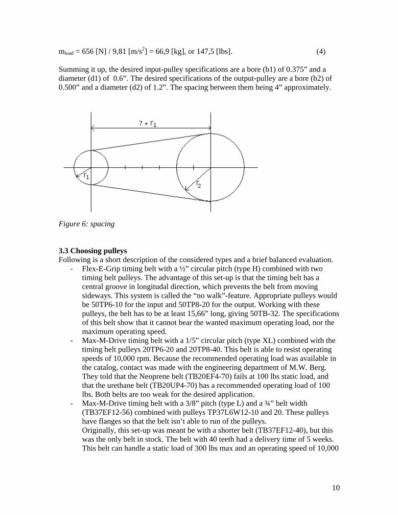
mload = 656 [N] / 9,81 [m/s2] = 66,9 [kg], or 147,5 [lbs]. (4) Summing it up, the desired input-pulley specifications are a bore (b1) of 0.375” and a diameter (d1) of 0.6”. The desired specifications of the output-pulley are a bore (b2) of 0.500” and a diameter (d2) of 1.2”. The spacing between them being 4” approximately.

Figure 6: spacing 3.3 Choosing pulleys Following is a short description of the considered types and a brief balanced evaluation.

- Flex-E-Grip timing belt with a ½” circular pitch (type H) combined with two timing belt pulleys. The advantage of this set-up is that the timing belt has a central groove in longitudal direction, which prevents the belt from moving sideways. This system is called the “no walk”-feature. Appropriate pulleys would be 50TP6-10 for the input and 50TP8-20 for the output. Working with these pulleys, the belt has to be at least 15,66” long, giving 50TB-32. The specifications of this belt show that it cannot bear the wanted maximum operating load, nor the maximum operating speed.

- Max-M-Drive timing belt with a 1/5” circular pitch (type XL) combined with the timing belt pulleys 20TP6-20 and 20TP8-40. This belt is able to resist operating speeds of 10,000 rpm. Because the recommended operating load was available in the catalog, contact was made with the engineering department of M.W. Berg. They told that the Neoprene belt (TB20EF4-70) fails at 100 lbs static load, and that the urethane belt (TB20UP4-70) has a recommended operating load of 100 lbs. Both belts are too weak for the desired application.

- Max-M-Drive timing belt with a 3/8” pitch (type L) and a ¾” belt width (TB37EF12-56) combined with pulleys TP37L6W12-10 and 20. These pulleys have flanges so that the belt isn’t able to run of the pulleys. Originally, this set-up was meant be with a shorter belt (TB37EF12-40), but this was the only belt in stock. The belt with 40 teeth had a delivery time of 5 weeks. This belt can handle a static load of 300 lbs max and an operating speed of 10,000

10

rpm. That makes it fulfilling all the wanted specifications, except for the length of the belt.

3.4 Choosing the belt Ideally, the two pulleys would be as close to each other as possible. This makes the free part of the belt (traveling between the pulleys) very short, and therefore very rigid (low mass, high eigenfrequency and a smaller piece of undamped material). On the other hand, if the two pulleys are too close to each other, the angle of entrance of the belt onto the pulley gets too high and can be a cause for slip and reduced belt life, as said before. Therefore, the spacing between the pulleys is chosen to be 4”. The chosen pulleys have a pitch diameter of 1.194” and 2.387”. From these data the belt length can be calculated.

slope2pulley1pulleybelt L*2r*r*L +π+π= (5) with Lslope the distance between the release of the belt at pulley1 and arrival at puley2. Lslope is calculated easily with Pythagoras’ rule.

))rr(4(L 22pulley1pulley

2slope −+= (6)

In this case, the optimal length Lbelt would be 13,715”, which makes TB37EF12-40 the best option. Unfortunately, this was not in stock. The first available belt was the TB37EF12-56, which is 21” long. Using the same formulas, the current spacing can again be calculated, and appears to be 7,7”. Choosing a bigger size for the pulleys was also discussed, but W.M. Berg didn’t have those in stock either. 3.5 Results A week later, W.M. Berg Manufacturing had some trouble with the payment, and one of the parts wasn’t in stock although they said it was. After a search in the region, Kaman Industrial Technology in West-Sacramento had just what we needed. Because a different type of oil pumps were ordered then originally specified the diameter of the shaft on the oil pumps was also different, 7/16” instead of ½”, so the pulleys ordered at W.M. Berg wouldn’t either. Kaman Industrial Technology sold bushings so that the pulleys could be mounted onto the 7/16” shaft, and if the originally specified pumps arrive, only these bushings have to be changed. After giving them the dimensions of the pulleys and the belt that I wanted, they helped find the right part numbers and ordered them for me. I ordered the 20LO50 pulley as the largest pulley and the 10LO50 as the small pulley, together with the 15” belt and the JA7/16 bushing. Two days later they were delivered and everything fitted as promised.

11

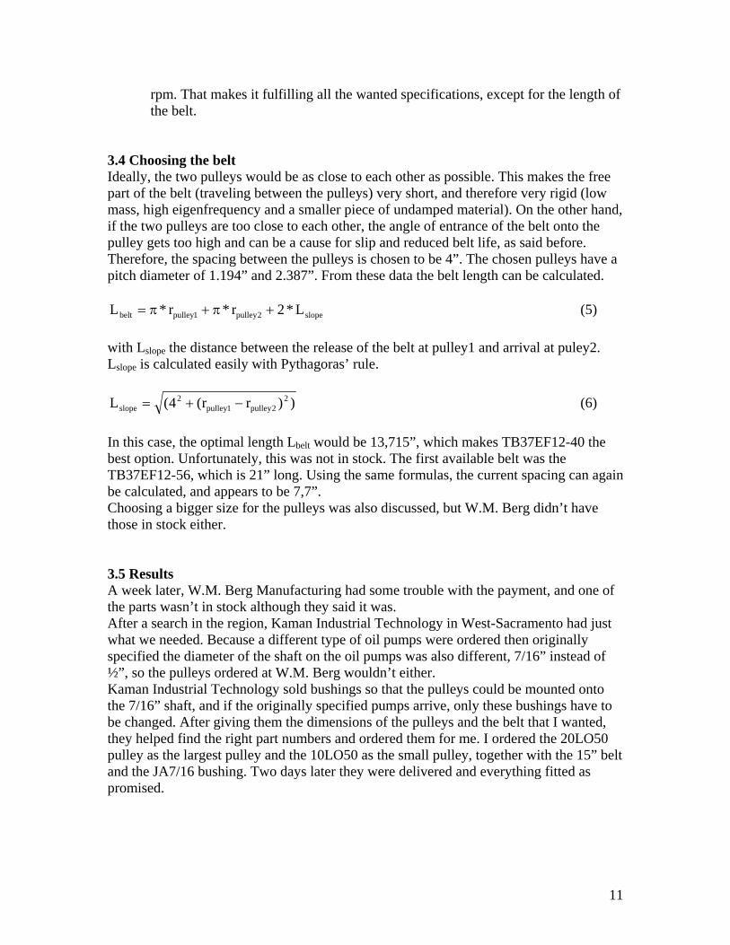
3.6 Mounting plate 3.6.1 Production The hydraulic pump and the electromotor have to be connected together with a mounting plate. In the complete set-up, two of these combinations are necessary. That means two electromotors and two hydraulic pumps. It is the easiest and cleanest to combine this all together into one. Various ideas were considered. Whatever is chosen, it has to be possible to disassemble or repair it quickly, it has to be as small and space-efficient as possible and it has to be light and preferably easy to manufacture. The best way to achieve all the goals is to take a simple sheet metal and drill holes and sleeves in it. The electromotor and the hydraulic pump determine all the sizes and dimensions. The length of the belt used is also known, which determines the spacing. The sleeves are needed just for small adjustments and for tensioning the belt.

Figure 7: Mounting plate for pump and motor. At this mounting, one electromotor and one hydraulic pump will be mounted. So two of these mounting plates are necessary. They will be mounted opposite of each other, with the electro motors and hydraulic pumps on the outside. For a good accessibility, the spacers between the metal plates are made from thread and a hollow tube. A 5” clearance is kept, so the belt and all the other parts can be changed if necessary. The belt should be adjusted so that there is a small tension on it, but not more than that. The motor and the pump should both rotate very easily.

12

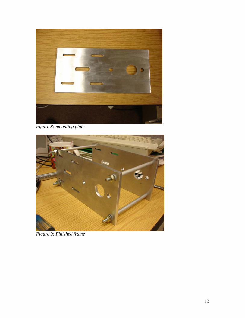
Figure 8: mounting plate

Figure 9: Finished frame

13

Figure 10: Complete setup 3.6.2 Current status After breaking down the oil pumps and ordering the original oil pumps as they were specified initially, the mounting plates had to be changed as well, to fit the new oil pumps in. Besides that, the pulleys from W.M.Berg were also useful now, because the new oil pumps did have the ½” shaft. Of these new mounting plates no drawing was made, they were just fabricated on the spot, using the old drawings, but with the specifications of the base of the new pumps. The rack itself, with the pumps and motors mounted to it, is attached to the test-rig with a aluminum plate. This plate has two slots were the spacer bars fit in, and two holes through which the bolts mount top the test rig itself. This prevents this setup from vibrating or falling over, and also releases any tension that might be on the hydraulic hoses.

14

4. Wiring I will discuss briefly how the sensors are wired, mainly for future reference. 4.1 Strain Gauge To connect the strain gauge to the PXI-1020, the following components are needed. From the strain gauge comes a 4-wire terminal.

- Black: Ground - Red: Input current 24V - Green: Positive output signal (V) - White: Negative output signal (V)

Both the output signal wires are connected to an amplifier, the Sensotec UV-10. This amplifier boosts the signal up to ± 10 Volts. This amplifier needs an outside power source of at least 18 VDC, two parallel placed batteries are used for this manner. These are also used for the power needed for the strain gauge itself. Unfortunately it seems that the peaks and drops in amperage influences the results by a significant noise. To solve this, a PCB has to be constructed that provides a continuous voltage at a continuous amperage. There also has to be taken special care to the isolation of the incoming signal. The output signals from the amplifier should go directly into the PXI-1020 box. The used slot, PXI-4472, is capable of handling input currents of + to – 10 V DC. Using the LabView program, it should be possible to collect data from the strain gauge. How this works, is discussed later on. 4.2 LVDT In order to measure the exact position of the pulley, a geometry sensor is necessary. For this purpose, the ISDT 20-K-2410 from P3 America [1] was ordered. This sensor has a stroke of 20 mm (10 mm on both sides from the electrical Zero Position) and an output of 0-10 Volts, also on both sides. The demodulator is built in. The current needed to built up the electrical field in the first coil is 24 Volts. That is the input current for the unit to operate. From the sensor comes a wire with five pins and a shield.

- Brown: Power input, 24 V - White: Signal ground - Green: Signal output, 0-10 V - Gray: Excitation ground - Yellow: Excitation ground, not connected - Shield: Ground, housing

On tip of the sensor is a small ball point, which will run on the edge of the pulley. Because the sensor’s output range varies between 0 and 10 Volts, and is always positive, the signal can be plugged into the PXI-1020 directly, without any form of conditioning.

15

4.3 Electromotor The hydraulic pumps are driven by an electromotor. Between the motor and the pump is a belt to reduce the ratio. The electromotor was available from a former project, and is a Emoteq BH03402-T01-H. Because this is a three-phase motor, the speed measurement has to be done with the output signal of three wires. There are also extra wires to indicate the sign of the signal. The wires have the following functions:

- Green: Ground (for the Hall-sensors, this means noise-free ground) - Blue: +5V Input for the Hall-sensors, again, noise-free - Brown: 1 or 0 discrete output signal, Phase A - Orange: 1 or 0 discrete output signal, Phase B - Yellow: 1 or 0 discrete output signal, Phase C - Red: -5V to +5V continuous output signal, Phase A - White: -5V to +5V continuous output signal, Phase B - Black: -5V to +5V continuous output signal, Phase C - Shield: Ground, housing Be careful, this is not a normal wiring, black isn’t the ground!

Figure 11: Wiring electromotor [3]

16

5. AMC 5.1 AMC For control over the electro motors that are in use for the actuation of the hydraulic pumps, an amplifier is needed. One of the possible controls is an AMC controller. I found a prefixed box, with two AMC controllers completely wired and mounted into it. Unfortunately, no description of the connectors on this box was provided. From the Internet I downloaded a user manual for the AMC B30 A40 Q, and identified all the pins and checked all the connections. I also adjusted all the switches and pot-settings. The necessary input power according to the specifications is variable between the 60 and 400 VDC. Two power supplies and two car batteries mounted in series provided the power for the initial tests, but they barely reached 70 VDC. So I ordered a new power supply capable of supplying 150 VDC for future use. After identifying all the pins at the connectors, I made new cables to go to the PXI chassis and to the electro motors. The new data cable to the PXI chassis ends at a RS232 connector, and the other side of the plug has all the wires that go into the SCB-68. This makes it easier to take everything apart, without having to unscrew all the wires out of the box. For future reference, I stored all the data in an excel-sheet. Now that I fully understood what all the pins on this box meant, I started working on connecting every sensor onto the PXI chassis. Then, with the system working, the amc’s were tuned properly, according to the ‘amc tuning’ file on the server. This means, that the motor spins at equal speed in both directions, and that the maximum speed is reached when the maximum speed signal is provided. 5.2 PXI First, all the sensors were one at a time connected to the PXI and calibrated and installed. For all these sensors, separate VI’s were made and stored on the hard disk, so that they can be used in the future if needed. These files can be found in the folder ‘subvis’ in the ‘Inline’ folder. From here on, all the necessary connections and the type (input or output, digital or analog signals) were written down, and I made a connection scheme to the PXI chassis. This scheme is also stored in an excel file, so it is easy to use and change if necessary. When I finally found out how I could connect all the sensors onto the PXI-chassis, and how they were all powered and what power supplies I needed to make everything work, I started connecting everything. First I made extension cables onto every sensor, all connected with the Deutsch connectors, so they can be used again in a different set-up in the future if needed, instead of using soldering connections, which is more difficult to disconnect and use again. Then I connected all the wires on the chassis, trying not to make a mesh of the wires, but a nice bundle instead, so that they can be disconnected and replace as easy as possible. First, I will explain the PXI-chassis and all it’s components. Then I will discuss the used connections and the reasoning behind these choices.

17

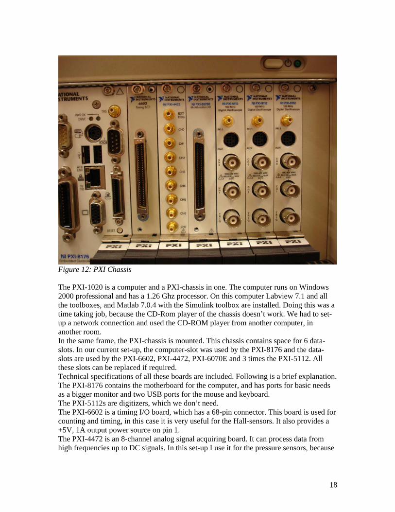
Figure 12: PXI Chassis The PXI-1020 is a computer and a PXI-chassis in one. The computer runs on Windows 2000 professional and has a 1.26 Ghz processor. On this computer Labview 7.1 and all the toolboxes, and Matlab 7.0.4 with the Simulink toolbox are installed. Doing this was a time taking job, because the CD-Rom player of the chassis doesn’t work. We had to set-up a network connection and used the CD-ROM player from another computer, in another room. In the same frame, the PXI-chassis is mounted. This chassis contains space for 6 data-slots. In our current set-up, the computer-slot was used by the PXI-8176 and the data-slots are used by the PXI-6602, PXI-4472, PXI-6070E and 3 times the PXI-5112. All these slots can be replaced if required. Technical specifications of all these boards are included. Following is a brief explanation. The PXI-8176 contains the motherboard for the computer, and has ports for basic needs as a bigger monitor and two USB ports for the mouse and keyboard. The PXI-5112s are digitizers, which we don’t need. The PXI-6602 is a timing I/O board, which has a 68-pin connector. This board is used for counting and timing, in this case it is very useful for the Hall-sensors. It also provides a +5V, 1A output power source on pin 1. The PXI-4472 is an 8-channel analog signal acquiring board. It can process data from high frequencies up to DC signals. In this set-up I use it for the pressure sensors, because

18

they give DC signals and I don’t want to have a big queue in the FIFO buffer of the PXI-6070E. The PXI-6070E is a multifunction analog and digital I/O board. It is capable of giving two analog output signals and collecting 16 analog input signals. All other pins are programmable, but don’t work in combination with the Labview DAQmx data assistant. Using these pins would give an additional (and unnecessary) programming effort. The signals processed by this board are distributed by the First In First Out (FIFO) principle. Using all the analog input channels can result in a large queue in the buffer, if the loop is to slow. Some signals have a low sample rate, which slows down the complete measurement. In this set-up, the 6070E is used the collect the data from the AMCs, the LVDT-sensor, both the torque-sensors and the temperature sensor. To connect sensors to the PXI, special connectors are needed. The PXI-4472 has only 8 channels, so the connectors are relatively big in size. It uses common plugs to connect to the sensors. The outside is the ground, on the inside is the signal. The PXI-6602 and 6070E however, use a special National Instruments 68-pin connector as connection to the outside. I found in the instruction manual the function of each pin and the corresponding pin and channel number. Various options are available to connect the sensors to this special connector, and I used the SBC-68 from NI, in combination with the data cable SH68-68-EP. This box has screw-terminals to connect all the wires from the sensors and is completely shielded for maximum noise reduction. These boxes are fused and provide ground for every analog input and output channel. I made this useful picture to help with connecting the wires to the boxes.

19

Figure 13: PXI slots The DAQassistant, a subprogram inside the LabView program, automatically selects the channel you can use for the desired measurement. For more information on all the programming in LabView see chapter 6 The PXI-1020 chassis is mounted into a rack, together with an additional screen (CRT) and the keyboard and mouse. This rack is moveable, since the power outlet is mounted onto the bottom of this rack as well.

20

Later on, when the test-rig is running fine, and the experimental phase is over, the basic idea is to move the rack over to the window, and raise the height of the screen so it can be monitored from the outside, while the rig is spinning. Because all the sensors have short wires, and need to be connected and disconnected very easily from the PXI chassis, without unscrewing every wire attached to the SCB’s, I made Deutsch connectors on every sensor, and made an extra wire that connects from these Deutsch connectors to the SCB’s. If the sensor is removed or replaced or something similar, this wire can stay into position. This appeared to be very helpful when we had trouble with the pressure sensors and with the Hall sensors.

21

6. LabView 6.1 LabView The computer program that is recommended by National Instruments to provide the entire user interface with the PXI-slots is called LabView. In this case, we used the latest version, called LabView 7.1. Because I never worked with this program before, and neither had one of my colleagues, I kept on running into all kinds of mistakes. NI provides a very good help line and support system, so most of the problems were solved within a day. The user interface consists of two panels, a block diagram, the not visible construction behind the other panel, which is called the front panel. The front panel is what you use and see while gathering data or controlling the output channels. Both panels are saved in one file, called a Virtual Instrument, or VI. First, I made VI’s for every single sensor. This was to test and calibrate them, and to have the building bricks for making more complex VI’s. For this latter purpose, I also changed all the VI’s in so-called subVI’s, which contain the connectors and are appear as one single block when used inside a bigger VI. This keeps the VI’s clean, and better to understand. For the rest of this part of my internship, I teamed up with Siddarth Shastri. We tried to make some VI’s with multiple channels and input and output combined. In order to get this working, we needed to decide in which order the PXI should collect and sent data, otherwise a queue would grow. The structure inside LabView is designed in a specific manner, which means that the board has to be ‘released’ by the software before it can start the next task. To release to board, all the DAQassistants had to be set to ‘one sample on demand’, and all the error-signals had to be wired in the order we wanted. After the one sample, the error signal then will release the board and move on to the next DAQassistant, which will be able to perform the next task. Furthermore, we needed to work with while-loops, to get the software repeating its task until the stop button is pressed. The while loop that controls the amc’s is made this way, that if the stop button is pressed, the error-signal immediately goes to outside the loop, to two DAQassistants who give a zero signal to the amc’s, so that the pumps stop immediately. Calibration. We also used LabView to calibrate all the sensors, because you can add scaling to the VI. To scale the pressure sensors, we compared the signal in voltage with the actual pressure as indicated by the analog pressure gauges mounted onto the hydraulic system. We wrote down the voltage values, and the according pressure values and put these values into Matlab, using the polyfit command >> v=[.6 1.3 1.42 1.6 1.65 1.87 2.06 2.25]; >> p=[15 700 850 1050 1100 1325 1500 1700]; >> a=polyfit(v,p,1) a = 1027.1 -606.96

22

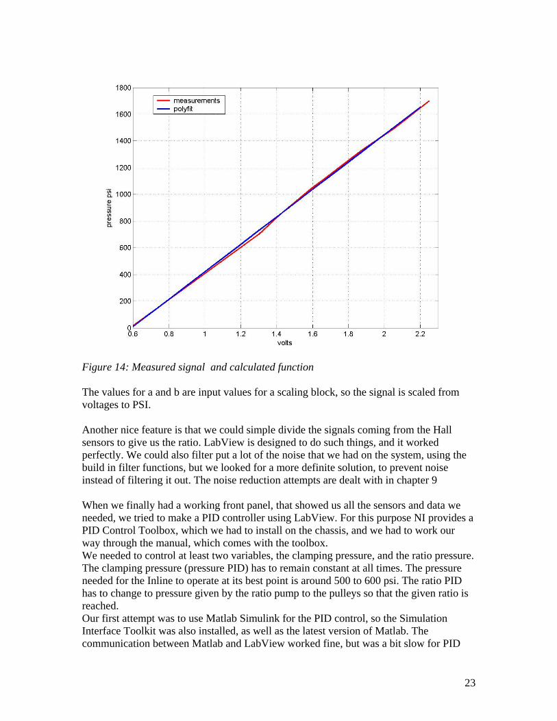
Figure 14: Measured signal and calculated function The values for a and b are input values for a scaling block, so the signal is scaled from voltages to PSI. Another nice feature is that we could simple divide the signals coming from the Hall sensors to give us the ratio. LabView is designed to do such things, and it worked perfectly. We could also filter put a lot of the noise that we had on the system, using the build in filter functions, but we looked for a more definite solution, to prevent noise instead of filtering it out. The noise reduction attempts are dealt with in chapter 9 When we finally had a working front panel, that showed us all the sensors and data we needed, we tried to make a PID controller using LabView. For this purpose NI provides a PID Control Toolbox, which we had to install on the chassis, and we had to work our way through the manual, which comes with the toolbox. We needed to control at least two variables, the clamping pressure, and the ratio pressure. The clamping pressure (pressure PID) has to remain constant at all times. The pressure needed for the Inline to operate at its best point is around 500 to 600 psi. The ratio PID has to change to pressure given by the ratio pump to the pulleys so that the given ratio is reached. Our first attempt was to use Matlab Simulink for the PID control, so the Simulation Interface Toolkit was also installed, as well as the latest version of Matlab. The communication between Matlab and LabView worked fine, but was a bit slow for PID

23

control. Besides that, it didn’t make the programming easier, because you had to change everything in two programs and then start compiling. After this attempt we learned that there should be a PID Control Toolbox available for LabView, traced this one down and installed it on the chassis. With this PID Control Toolbox we tried to set up a control for the pressure and for the ratio. Because testing a PID controller on the real life system is a bit complicated, we made a small test set-up with two motors mounted into a frame and controlled by AMC’s, with two Hall sensors each monitoring the speed of one motor and with a pressure sensor used for the feedback loop.

Figure 15: temporary test set-up. This took some time, because we had to figure out how these AMC’s had to be set-up. These AMC’s (BA40A8) are different from the ones we use in the test-rig. They were actually easier to connect, but could also handle less power. For this purpose that didn’t matter. Still, we had to go through the manual to connect every wire. First we made the feedback loop for the ratio. One motor was given a continuous speed (master) and the other motor had to follow at the desired ratio (slave). Disturbances were introduced, as changing the masterspeed, the desired ratio, noise on the Hall signal, blocking the Hall sensors, and all the time the system had to remain stable. After trail-and-error, this all ran fine. Having the ratio pid.vi finally under control, we made a new test setup for the pressure pid. In order to work on this, we connected a pressure sensor to the PXI, and one AMC with electromotor. In the VI, we used a numeric value for the desired pressure as set point, and compared that with the measured pressure, which we change by pushing the sensor with a pencil. The change of speed and direction of the electromotor was the controlled signal. We got this one working as well, you could see the speed and direction of the electro motor changing as we brought the measured pressure closer to, or over the desired pressure.

24

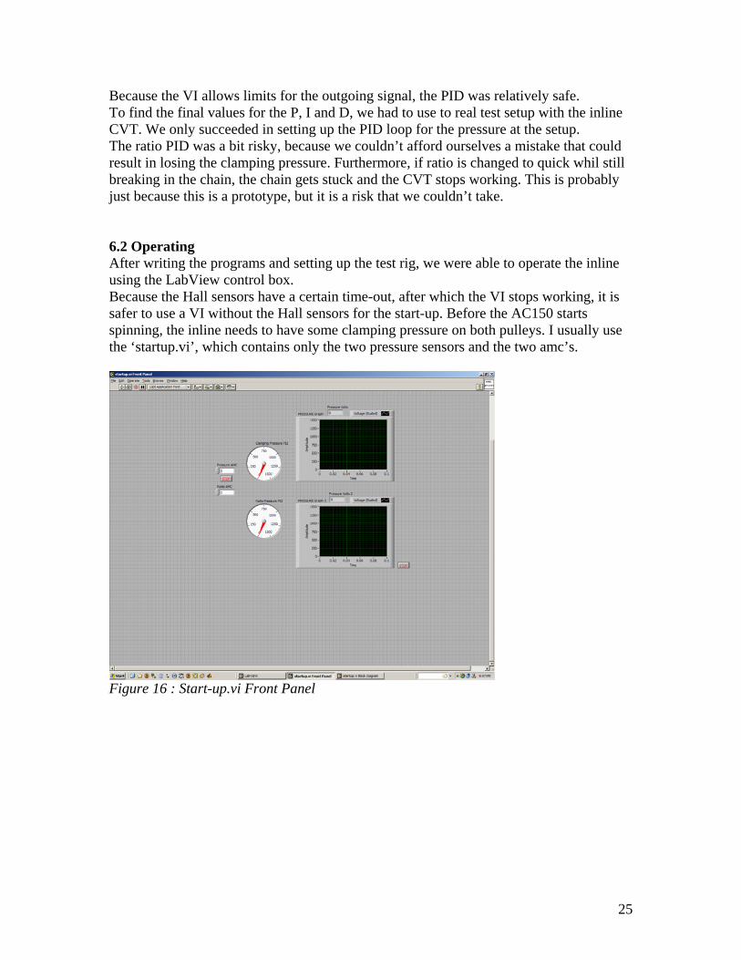
Because the VI allows limits for the outgoing signal, the PID was relatively safe. To find the final values for the P, I and D, we had to use to real test setup with the inline CVT. We only succeeded in setting up the PID loop for the pressure at the setup. The ratio PID was a bit risky, because we couldn’t afford ourselves a mistake that could result in losing the clamping pressure. Furthermore, if ratio is changed to quick whil still breaking in the chain, the chain gets stuck and the CVT stops working. This is probably just because this is a prototype, but it is a risk that we couldn’t take. 6.2 Operating After writing the programs and setting up the test rig, we were able to operate the inline using the LabView control box. Because the Hall sensors have a certain time-out, after which the VI stops working, it is safer to use a VI without the Hall sensors for the start-up. Before the AC150 starts spinning, the inline needs to have some clamping pressure on both pulleys. I usually use the ‘startup.vi’, which contains only the two pressure sensors and the two amc’s.

Figure 16 : Start-up.vi Front Panel

25

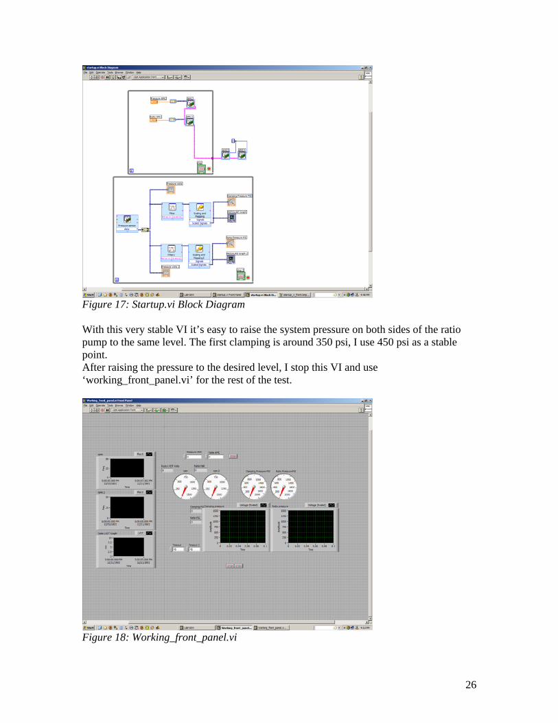
Figure 17: Startup.vi Block Diagram With this very stable VI it’s easy to raise the system pressure on both sides of the ratio pump to the same level. The first clamping is around 350 psi, I use 450 psi as a stable point. After raising the pressure to the desired level, I stop this VI and use ‘working_front_panel.vi’ for the rest of the test.

Figure 18: Working_front_panel.vi

26

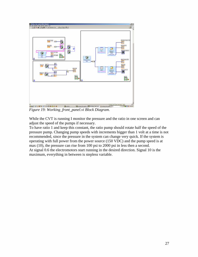
Figure 19: Working_front_panel.vi Block Diagram. While the CVT is running I monitor the pressure and the ratio in one screen and can adjust the speed of the pumps if necessary. To have ratio 1 and keep this constant, the ratio pump should rotate half the speed of the pressure pump. Changing pump speeds with increments bigger than 1 volt at a time is not recommended, since the pressure in the system can change very quick. If the system is operating with full power from the power source (150 VDC) and the pump speed is at max (10), the pressure can rise from 100 psi to 2000 psi in less then a second. At signal 0.6 the electromotors start running in the desired direction. Signal 10 is the maximum, everything in between is stepless variable.

27

7. Power source 7.1 Power source The AMC’s are able to handle high voltages, up to 400 VDC. The electromotors are also able to run on high voltages, and the higher the voltage, the higher the speeds the electromotors will be able to reach. In our initial, temporary setup, we used a combination of two car batteries and two portable lab power sources, all put in series, to reach the desired 60 VDC to get the system running. This wasn’t a very proper power source. It had weak connections, bad isolation, and the car batteries were at the end of their lives, so they lost their charge quickly. We decided that we needed a real lab power source. Our demands were a stepless adjustable, 0 to 150 VDC power source, which should have an input power from the net, so that would be 110 VAC. After some internet research and some telephone calls, and numerous quotes, we decided to go for the Sorensen DCR150-18B from Testmart.com.[7] After more than a week, they contacted us about the displays on the power source. It was a refurbished one, and one display was digital, and the other display was analog. We agreed with that. Then, they contacted us with the announcement that the input power was 208 VAC, 60 Hz, 3 phase, instead of the promised 110 VAC, 2 phase. We still accepted it, because we wanted to continue our research, but we agreed on never doing business with this company again.

28

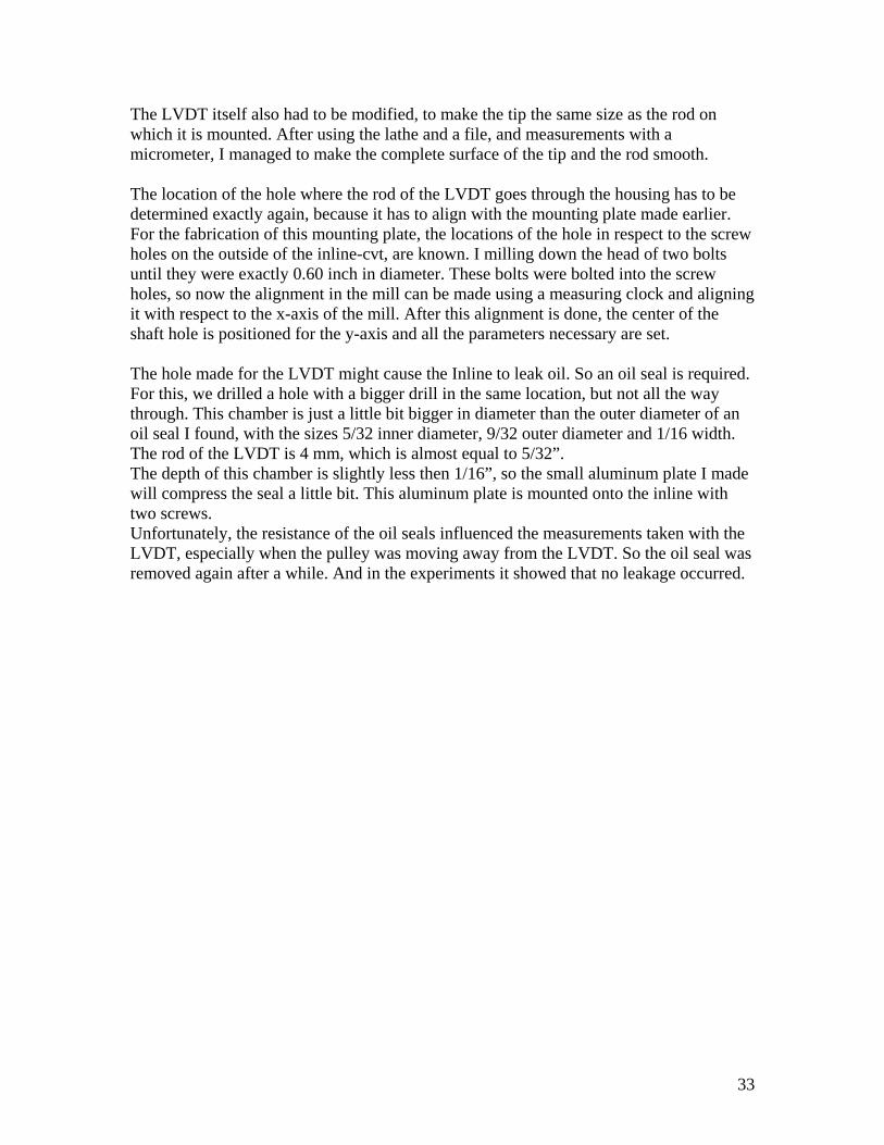
8 Mounting sensors Following is a short description of the sensors that I mounted onto the set-up, and how they are connected to the data acquisition box. 8.1 Strain gauge The strain gauge is already mounted onto the dynamometer. Unfortunately, the distance between the center of the axis of the dynamometer and the middle of the strain gauge measuring block is unknown, and has yet to be determined. Before measuring the distance, with all its uncertainties, a thorough search through all the papers of the previous group will be performed, in order to find their findings. If nothing is found in the reports and papers, a measurement has to be made. 8.2 LVDT The ISDT20-K-2410 is supplied without any form of mounting. A custom made solution has to be made. The sensor itself is completely smooth on the outside, making it hard to mount on a surface. A possible solution is drilling a hole in the CVT housing and putting the tip of the sensor through it, sealing it with an oil seal. To solve the actual problem, fixing it onto the housing, a mount has to be made from scratch. For this purpose a mount was already made with a cylindrical shape. I only had to complete the milling until it reached the desired size. This will fit around the sensor and hold the sensor with a hose clamp. The cylinder will then be bolted onto an aluminum plate. This plate is shaped to fit the housing. While the housing is hand-build, the exact locations of the screw holes were not sure. Therefore, I made some measurements with the 3D CMM available in the machine. With these measurements, and some calculations, a CNC-program was written and the mounting plate was milled out of a ¼” thick aluminum plate in the machine shop. The exact location of the hole were the LVDT had to fit through the mounting plate had to determined very carefully, because the edge of the pulley where the tip of the LVDT has to touch is very small (3 mm). From the drawings of the inline available on the server the diameter of the pulley could determined and also the position of this hole with respect to the central where the shaft comes out of the housing. The CNC program is available for future reference.

29

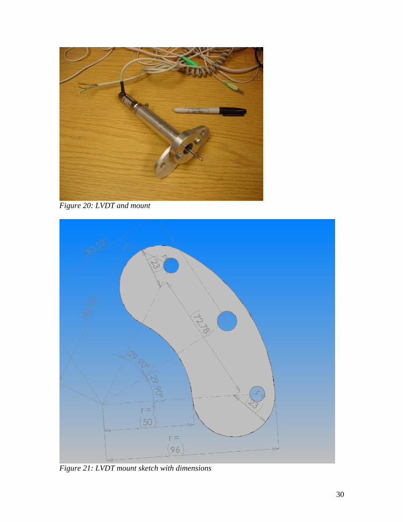
Figure 20: LVDT and mount

Figure 21: LVDT mount sketch with dimensions

30

For the next set-up, a better solution is found. Because the cylinder doesn’t statically determines the position and grip of the sensor. A better way to hold a cylindrical shape (like the sensor) is to clamp it in a V-shaped mount and hold it down with a flat surface. Then the touching surfaces are all perpendicular to the radius of the cylinder, and the cylinder will be clamped in three places. This makes this type of holding statically determined. If this clamp is made, I should look like this:

Figure 22: sketch of mount Note: The two bolts should go through the block, and are secured with the nuts on the other side. Of course mounting this block onto the housing with three screws would be better (statically determined), but that also costs space and material. Because the LVDT isn’t supposed nor designed to be subject to high forces, this mounting will do just as well. The dimensions for this block are determined by the size of the sensor. Because the sensor has to be tightened between the two blocks, the gap has to be very small. Also, the edges have to be perpendicular to the radius of the sensor’s cylindrical shape. This means, with a radius of 10 mm, that the dimensions for the v-shape are easily calculated using simple mathematics.

31

Figure 23: simple mathematics

mm142*10)45cos(

RB ≈== (7)

The gap between the flat surface and the V-shaped groove should be kept very small, so 2 mm is taken. The other sizes are determined by the space needed for the bolts and holes that have to be made into the mount to fix it to the housing of the CVT.

Figure 24: Sketch with dimensions (in mm)

32

The LVDT itself also had to be modified, to make the tip the same size as the rod on which it is mounted. After using the lathe and a file, and measurements with a micrometer, I managed to make the complete surface of the tip and the rod smooth. The location of the hole where the rod of the LVDT goes through the housing has to be determined exactly again, because it has to align with the mounting plate made earlier. For the fabrication of this mounting plate, the locations of the hole in respect to the screw holes on the outside of the inline-cvt, are known. I milling down the head of two bolts until they were exactly 0.60 inch in diameter. These bolts were bolted into the screw holes, so now the alignment in the mill can be made using a measuring clock and aligning it with respect to the x-axis of the mill. After this alignment is done, the center of the shaft hole is positioned for the y-axis and all the parameters necessary are set. The hole made for the LVDT might cause the Inline to leak oil. So an oil seal is required. For this, we drilled a hole with a bigger drill in the same location, but not all the way through. This chamber is just a little bit bigger in diameter than the outer diameter of an oil seal I found, with the sizes 5/32 inner diameter, 9/32 outer diameter and 1/16 width. The rod of the LVDT is 4 mm, which is almost equal to 5/32”. The depth of this chamber is slightly less then 1/16”, so the small aluminum plate I made will compress the seal a little bit. This aluminum plate is mounted onto the inline with two screws. Unfortunately, the resistance of the oil seals influenced the measurements taken with the LVDT, especially when the pulley was moving away from the LVDT. So the oil seal was removed again after a while. And in the experiments it showed that no leakage occurred.

33

9 Noise 9.1 General As always, noise plays an important role in measurements and data acquisition. This is especially true in this case. The noise measured on the Hall sensor signal was so large, that the original signal wasn’t visible anymore. While setting up the test rig for the first initial tests, we didn’t pay particular attention to noise reduction. Of course, all the usual precautions were taken into account. So if a sensor had shielded wire, this shielding is attached to the ground. All the ground signals coming from the sensors were connected to the LabView box, because according to the description, LabView would use the noise from this channel to subtract it from the analog input channel. That means that all the ground signals had to be connected so that they would be paired with their according input channel. As far as the pressure sensors and the temperature sensor, we were only interested in an indication of the height of the signal, not in the exact number. While spinning the AC150, the noise on the signal wires became incredibly high. To reduce this to a reasonable amount, we used two approaches. One was to isolate every wire and every sensor as much as we could, the other was to find the source of the noise and eliminate it. 9.2 Protecting against noise. The hall sensors came with unisolated wires. The best solution was to cut the wires off to approximately three inches long, and then connecting a isolated, shielded wire with a deutsch connector to them. Of course, the unisolated part will still pick up some noise, but it caused a huge reduction in noise level. The shielded outside out of the temperature sensor was covered with a plastic hose, so it didn’t touch the test rig anymore. Still, there was too much noise on the Hall sensor signals. We tried to protect the Hall sensors with braided hoses around it attached to the ground, with a steel casing and with holding metal sheets in front of them, and finally we came to the conclusion that we had to go for the second approach, trying to eliminate the cause of the noise. 9.3 Noise source We were afraid that the tip of one of the Hall sensor might be touching a nut inside the CVT, so we milled down the threat of the tip. This didn’t make any difference. Another thing is that all the components of the Inline are attached to the test rig and each other. So all the noise that’s on the set-up travels freely from one component to another. We tried to get all the ground wires together in one spot, so they don’t influence each other. Because we didn’t have so much noise when the AC150 wasn’t running, we suspected the source of the noise to be either the AC150 or its control box. A very obvious source for the noise was the unshielded power line going from the control box to the AC150. This wire provides the high voltage in three phases in very high frequencies to the AC150 electro motor. This high frequency is necessary to get the high efficiency that was needed when the AC150 was still mounted into a car.

34

To isolate this cable, we decided to build a cage of Faraday around the line. We expected the noise to be electromagnetical, because it is caused by the high frequency voltage changes. We found a suitable length of exhaust pipe, cut it open lengthwise, fitted it around the power line and closed it again using aluminum tape. All the separate parts are connected together using copper wire and the end of the copper wire is attached to the ground.

Figure 25: Exhaust as shield around power line. This reduced the noise by a reasonable amount. When the system was finally running again (all kinds of other improvements and changes are made between runs, thus lowering the amount of runs we were able to make) we tried to find the sources for the electromagnetical noise by using a coiled wire and measure the millivolts generated by the noise. The control box generated almost 5 mV, while under normal circumstances, without any machine switched on, the noise was around 1,5 to 2 mV. The AC150 itself apparently also generates some noise, around 3 mV was measured in the direct surrounding of this electromotor. 9.4 Recommendations We tried to connect all the ground wires on one fixed point, but in the lab there was no good grounding available. A large, long, metal pin put deep into the earth could provide a good grounding. It would be a good idea to think about making a ground like this, separate from the test rig itself. This metal pin should not be in contact with anything in the lab except for the ground wires. That would make it a noise free ground, without any change of noise coming from this ground and going into the setup. A second, more important recommendation is shielding the control box for the AC150. It is generating so much noise, it should be covered with a thick metal casing. We didn’t have the time to come up with a definitive solution, but somebody should be working on this one in the near future.

35

Conclusion After 4,5 months of work, we may conclude that we didn’t do what we came for. We don’t have measurements of the efficiency, nor of the slip. Still, we did a lot of useful work, and we can’t say we don’t have any results to show. We set-up the test-rig, we ordered all the necessary parts, we assembled all the sensors and learned how to work with some computerprograms like LabView and Superflow. The set-up as it is right now is ready to start the testing, only the noise from the control box is holding that back. As soon as that is fixed, it is possible to measure and calculate the efficiency and dynamic slip of the Inline-CVT.

36

Sources [1] Fundamentals of machine component design, Second Edition, Robert C. Juvinall and Kurt M. Marshek, John Wiley and Sons Inc., New York, 1991 [2] http://www.efunda.com [3] From Emoteq.com http://www.emoteq.com/downloads/High%20Speed%20Motors%20Selection%20Guide2.zip[4] ‘Polytechnisch zakboekje’, Prof. Ir. P.P.H. Leijendeckers, 48th print, Elsevier, Arnhem, 1998 [5] LabView Course Manual, I and II. [6] http://www.ni.com[7] http://www.testmart.com[8]

37

Thanks Special thanks to Siddarth Shastri and Tashari El-Sheikh for all their help with everything in and outside the office, to Prof Andrew Frank for this opportunity, Simone Keultz for the visa, the NI helpdesk for their good support, all the other Team Fate members for their help and my roommates for their support and friendship.

38