a thermoacoustic characterization of a rijke-type tube
TRANSCRIPT
A Thermoacoustic Characterization of a Rijke-type
Tube Combustor
Lars Nord
Thesis submitted to the Faculty of the
Virginia Polytechnic Institute and State University
in partial fulfillment of the requirements for the degree of
Master of Science
in
Mechanical Engineering
Dr. William R. Saunders, Chair
Dr. Uri Vandsburger, Co-Chair
Dr. Ricardo Burdisso
February, 2000
Blacksburg, Virginia
Keywords: acoustics, chemiluminescence, combustion, flame instabilities
A Thermoacoustic Characterization of a Rijke-type
Tube Combustor
Lars Nord
Dr. William R. Saunders, Chair
Dr. Uri Vandsburger, Co-Chair
Department of Mechanical Engineering
(ABSTRACT)
Pressure pulsations, or thermoacoustic instabilities, as they are called in the research
community, can cause extensive damage in gas turbine combustion chambers. To
understand the phenomena related to thermoacoustics, a simple Rijke-type tube
combustor was built and studied. Extensive experimental results, as well as theoretical
analyses related to the Rijke tube are presented in this thesis. The results, attributable to
both the analyses and the experiments, help explain all the phenomena affecting the
acoustic pressure in the combustor. The conclusion is that there are three separate yet
related physical processes affecting the acoustic pressure in the tube. The three
mechanisms are as follows: a main thermoacoustic instability in accordance to the
Rayleigh Criterion; a vibrating flame instability where the flame sheet exhibits mode
shapes; and a pulsating flame instability driven by heat losses to the flame stabilizer. All
these instabilities affect the heat released to the gas in the combustor. The energy from
the oscillating heat couples with the acoustics of the volume bounded by the tube
structure. The experimental results in the study are important in order to obtain model
parameters for prediction as well as for achieving control of the instabilities.

To Ragnhild

iv
Acknowledgements
I wish to thank the members of both the Virgina Active Combustion Control
Group (VACCG) and the Reacting Flows Laboratory (RFL) for help during the progress
of this thesis. A special thanks goes out to the three professors in my committee, Dr. Uri
Vandsburger, Dr. William Saunders, and Dr. Ricardo Burdisso for all the help and
support they provided during my time at Virginia Tech. I would also like to thank fellow
students Ludwig Haber, who set up the optics system utilized in the experiments for this
thesis; Chris Fannin, who set up a bench-top experiment for studying a vibrating flame
phenomenon analyzed in the thesis; Bryan Eisenhower for general help with the tube
combustor; John Richards for fabrication and calibration of pressure transducers; and
Donald Grove for thermocouple fabrication and setup. A number of helpful discussions
and general help in the laboratory have been provided from students Vivek Khanna and
Steve Lepera. For assistance when collecting all the data presented in this thesis, Jesse
Seymore has been very important and without Jesse the work would have taken much
longer. For reviewing the thesis I thank Professor J. Lawrence McLaughlin and co-
worker Helmer Andersen. Finally I would like to thank my parents Stig & Linnéa Nord,
as well as Halley Orthmeyer for all the emotional support they have given me during the
time I spent working on this thesis.

v
Table of Contents
Chapter 1 Introduction 1 1.1 Background 1
1.2 Objectives and Scope 2
1.3 Technical Approach 3
Chapter 2 Literature Review and Theoretical Background 4
2.1 Literature Review 4
2.1.1 Thermoacoustics and Rijke-type Tube Combustors 4
2.1.2 Vibrating and Pulsating Flames 6
2.1.3 Review Articles 8
2.2 Theoretical Background 9
2.2.1 Solution of the Wave Equation for a Closed-Open Duct 9
2.2.2 The Rayleigh Criterion 13
2.2.3 Definition of Equivalence Ratio for Methane with Air as Oxidizer 14
Chapter 3 Experimental Systems and Methods 16
3.1 Overview of Experimental Components 16
3.2 Tube Combustor 17
3.3 Pressure Transducers 19
3.4 Thermocouples 20
3.5 Optical System for Chemiluminescence Measurements 21
3.6 Mass Flow Meters 23
3.7 Data Acquisition Equipment 24
Chapter 4 Rijke-tube Thermoacoustic Characterization 26
4.1 Acoustic Pressure 26
4.1.1 Limit Cycle and Harmonics 28
4.1.2 Subharmonic Response 29
4.1.3 Subsonic Instability 37
vi
4.2 Chemiluminescence Measurements 42
4.3 Comparison of Pressure and Chemiluminescence Spectra 43
4.4 Axial Temperature Profiles 44
4.5 The Operational Characteristics of the Tube Combustor 45
4.6 Extensive Mapping of the Operating Region 46
4.7 Database on the World Wide Web 53
4.8 Resonance Frequencies 53
Chapter 5 Conclusions and Future Work 58
5.1 Conclusions 58
5.2 Future Work 59
References 61
Appendix A Pressure Power Spectra for Constant Equivalence Ratio 66
Appendix B Pressure Power Spectra for Constant Flow Rate 87
Appendix C OH* Power Spectra for Constant Equivalence Ratio 108
Appendix D OH* Power Spectra for Constant Flow Rate 129
Appendix E Axial Temperature Distributions for Constant
Equivalence Ratio 150
Appendix F Axial Temperature Distributions for Constant Flow Rate 171
Vita 192
1
Chapter 1 Introduction
1.1 Background
In a dry low NOx-emission gas turbine, problems with pressure pulsations can
occur in the combustion chamber. The pressure pulsations can couple with the structure
and cause violent vibrations to the extent that the whole gas turbine fails. In the past, this
was not a major problem because of the use of diffusion flames in addition to the
secondary air supplied through holes in the combustor walls. Modern gas turbines with a
dry low NOx-system use premixed air-fuel so that it is no longer necessary to add
secondary air. The cooling schemes have also changed; convective cooling is now often
used instead of film cooling. This process made almost all the holes in the combustor
walls vanish and thus the chamber essentially became a resonator with very little
attenuation. To limit the production of NOx, the flame is kept as lean as possible.
However, this leads to a more unstable flame, with oscillating heat release that couples
with the acoustics of the chamber. Therefore, in the past several years there has been a
keen interest in the study of thermoacoustic (TA) instabilities, which is defined as the
coupling between the heat release rate and the acoustic pressure. This problem has been
studied for over a century. It began in 1877 when Lord Rayleigh described how the
balance between acoustic dissipation and acoustic excitation, due to unsteady heat
transfer, can lead to a self-excited, unstable acoustic response. The criterion, called the
Rayleigh Criterion, have been studied by several researchers including Blackshear
(1953), Putnam (1971), and Joos and Vortmeyer (1986). This fundamental perspective of
energy balance is very useful in many ways, but it does not provide sufficient detail to
explain all of the characteristics that may be observed during unstable TA response of a
combustor.
A Rijke-type tube, named after an experimental setup presented by Rijke (1859),
is a fundamental setup for the study of thermoacoustic instabilities. Rijke tubes and
related devices have been studied by Putnam (1971), Bailey (1957), and a review of the
field was presented by Raun, Beckstead, Finlinson, and Brooks (1993). The geometry of
a Rijke tube, typically with a large length-to-diameter ratio, is much simpler than the
Lars Nord Chapter 1 Introduction 2
geometry of a full-scale combustor used in gas turbines. The large length-to-diameter
ratio basically makes the problem one-dimensional which makes the acoustics easier to
analyze, and, since there are no sudden area changes, the shedding of vortices is limited
compared to a dump combustor. It is therefore possible to isolate specific phenomena
related to thermoacoustics more effectively than in a full-scale combustor. The flame
shape is typically a flat flame compared to the much more complex flames in gas turbine
combustion chambers which means the flame-acoustic interaction also is less involved.
In the past, researchers have studied specific phenomena related to this area.
Many researchers have studied the thermoacoustic instability in terms of amplitude and
frequency. They have also studied how different parameters affect the TA instability.
Others have concentrated on flame-acoustic interaction in terms of pulsating flame
instabilities and vibrating flames. In this thesis, an effort is made to qualitatively
understand all the phenomena that have some visual effect on the pressure power
spectrum in a Rijke-type tube with a burner-stabilized premixed flame.
1.2 Objectives and Scope
The overall objective of the research conducted by Virginia Active Combustion
Control Group [VACCG] was to increase the understanding of thermoacoustic
instabilities to be able to predict and provide active control of the instabilities in a full-
scale combustor. To achieve that, models for the TA instabilities, including flame
dynamics, fluid dynamics, and acoustic-flame interactions, have to be developed.
The part of the project presented in this thesis involves the study of a simple tube
combustor. VACCG members have investigated a number of theories associated with the
phenomena occurring in the combustor. The research presented in this document will,
with the help of extensive experimental data, strengthen the suggested theories. The
experiments conducted will also serve as a database for the VACCG and the research
community within this field. In addition the collected data can be helpful in the
development of reduced-order modeling schemes that provide adequate prediction
capabilities for the occurrence of thermoacoustic instabilities. The experimental
Lars Nord Chapter 1 Introduction 3
investigation included a mapping of the tube combustor in terms of acoustic pressure,
temperature distribution, and chemiluminescence for the whole operating region.
1.3 Technical Approach
A very simple combustion process was selected to facilitate initial studies of
thermoacoustic instabilities at Virginia Tech. The tube combustor is similar to a Rijke
tube except that the boundary conditions are closed-open versus open-open. According
to the Rayleigh Criterion this leads to a TA instability of the 2nd acoustic mode when the
flame is placed at the middle of the tube. There are some important limitations associated
with the study of TA instabilities in Rijke tubes versus real, full-scale combustors.
Primarily, the fluid dynamic coupling is not important, as there are no vortical structures
in the tube flow that can cause periodic heat release. This leads to easier studies of the
features that were the focus of this test device. Specifically, the tube combustor was
intentionally selected to eliminate coupling between TA instabilities and flow-
instabilities. This thesis will, using frequency-domain formats, examine the observed
acoustic and thermal-proportional response characteristics with interpretations based on
the measurements viewed. There is a large amount of information that resides in the
spectral representations of any dynamic system response measurements for linear or
nonlinear systems. The information supports descriptions of physical phenomena
responsible for unique spectral features. Therefore, it can be helpful to discern the details
of the thermoacoustic pressure signatures for both dynamic modeling and system
monitoring in any combustor system.
4
Chapter 2 Literature Review and Theoretical Background
2.1 Literature Review
This literature review is not intended to be complete as far as all the literature that
has been produced in the area of dynamics in Rijke tube combustors. The purpose of the
review is to give a background to this thesis and to give some insight into the work that
has been conducted in the research areas presented in the following sections.
2.1.1 Thermoacoustics and Rijke-type Tube Combustors
The first published experiments regarding Rijke tubes were conducted by Rijke
(1859) after whom the type of tube is named. He used an open-open tube and had a wire-
gauze to locally heat up the air in the tube. By doing this, the tube produced a sound
close to the fundamental tone of the tube. An explanation of the phenomena was
published by Rayleigh (1877), (1878), where he states “If heat be given to the air at the
moment of greatest condensation, or taken from it at the moment of greatest rarefaction,
the vibration is encouraged.” This statement is now known as the Rayleigh Criterion.
Putnam and Dennis (1953) studied three combustion systems exhibiting acoustical
oscillations: 1) an open-open tube with a premixed flame, 2) a closed-open tube with a
premixed flame, and 3) a closed-open tube with a diffusion flame. They concluded from
tests and from the analysis that oscillations were amplified when two requirements were
fulfilled simultaneously: First, an oscillating component of the heat release was in phase
with the pressure variation, and second, the point of heat release was close to a point of
maximum pressure amplitude in the combustor. By studying different configurations,
they added knowledge to the field by describing the amount and type of change in
apparatus configuration necessary either to eliminate or encourage oscillations. In the
appendix of Putnam and Dennis’s paper, a thermodynamic treatment of the phase
requirement between rate of heat release and pressure (the Rayleigh Criterion) was
presented. Putnam and Dennis (1954) made an investigation regarding a combustion
chamber with a mesh-screen flame holder. The exhaust gases passed out through a
converging nozzle and a stack. The depth of the flame holder and the length of the stack
Lars Nord Chapter 2 Literature Review and Theoretical Background
5
could be varied. A theory for the gauze tones produced was also presented. Putnam
presents these investigations, and much more information, in his book “Combustion
Driven Oscillations in Industry” (1971), where he states the Rayleigh Criterion in an
integral form. He also concluded that the condition required for combustion driven
oscillations to occur is determined by the integral ∫ )( tphd ω . Here p is the acoustic
pressure, h the unsteady part of the heat release, and ω the angular frequency. Blackshear
(1953) explained in detail the mechanism whereby the heat addition can drive or damp an
oscillation. In the experimental work he examined the effect of a flame on a standing
wave system by measuring the ability of the flame to damp an imposed standing wave
rather than to examine spontaneous excitation. A system, which was either closed-closed
or closed-open, was used, and the flame’s role was investigated by considering the
following variables: fuel-air ratio, inlet temperature, flame holder position, sound
amplitude, and inlet velocity. Bailey (1957) used an open-open tube to study flame-
excited oscillations. His results were in agreement with the Rayleigh Criterion. Joos and
Vortmeyer (1986) investigated how the Rayleigh Criterion is satisfied with superimposed
oscillations in situations when more than one frequency is excited. To do this, they
conducted simultaneous recordings of oscillations in the sound pressure, sound particle
velocity, and energy. For measurements of the heat release rate oscillation, OH*
radiation was studied. OH* is excited OH-radicals which, when going from their excited
state to their ground state, emit light, and are assumed to be proportional to the heat
released. “The Spectroscopy of Flames” by Gaydon (1974), a paper by Diederichsen and
Gould (1965), and the thesis “An Investigation Into the Origin, Measurement and
Application of Chemiluminescent Light Emissions from Premixed Flames” by Haber
(2000) provide more insight into this area. In accordance to the Rayleigh Criterion, Joos
and Vortmeyer found self-excited oscillations when the sound particle velocity preceded
the sound pressure. This was the case when only one frequency was excited. However,
when more than one frequency was excited the sound particle velocity phase, in relation
to the sound pressure phase, changed with time. The sound particle velocity phase lagged
behind the pressure at some stages; however, the oscillations were still sustained. Their
conclusion was that it is sufficient for sustained oscillations to fulfill the Rayleigh
Criterion temporarily.

Lars Nord Chapter 2 Literature Review and Theoretical Background
6
An extensive theoretical investigation was conducted by Bloxsidge, Dowling, and
Langhorne (1988) in conjunction with an experimental investigation by Langhorne
(1988). Their objective was to predict the frequency and onset fuel-air ratio for
oscillations to occur in practical geometries. They developed a model for the dynamic
behavior of the flame in response to an unsteady velocity field. The theoretical
predictions were then tested against experimental data. They found that the predicted and
measured frequencies were within 6 Hz and that the theory was able to predict trends in
variations in frequency as either equivalence ratio, inlet Mach number, or duct geometry
were changed. The oscillation frequency shift, with equivalence ratio, showed a non-
linear behavior both in the experiments and in the calculations. The frequency
dependence on the inlet Mach number showed a linear effect. Cho, Kim, and Lee (1998)
conducted a parametric study, with measurements of acoustic pressure and flame
radiation in various conditions in order to understand the effect of physical parameters,
such as Reynold’s number and equivalence ratio, in a ducted premixed flame burner.
They concluded that Reynold’s number neither affects the maximum pressure peak nor
the fundamental frequency of the system to any large extent. The equivalence ratio,
however, was an important parameter in terms of the maximum pressure peak and the
fundamental frequency.
In summary, it can be noted that the primary role of the studies of Rijke-type
tubes throughout the literature have either been related to the Rayleigh Criterion, in terms
of confirming it and/or extending it, or they have been related to parametric studies,
where the effects of fuel-air ratio, fluid velocity, flame holder position, and duct
geometry were examined.
2.1.2 Vibrating and Pulsating Flames
Both vibrating and pulsating instabilities are seen in burner-stabilized premixed
flames. Vibrating flames, also called wrinkled flames, are cellular instabilities and are
typically seen at Lewis numbers below unity. Pulsating instabilities, however, occurs at
Lewis numbers above unity and are one-dimensional instabilities in the axial direction of
the combustor system.
Lars Nord Chapter 2 Literature Review and Theoretical Background
7
Markstein (1964) published articles on non-steady flame propagation. Among the
relative articles is Markstein’s “Perturbation Analysis of Stability and Response,” in
which he discussed vibrating flames which is examined further in Chapter 4 of this thesis.
Margolis (1980) also discussed pulsating instabilities. He showed, with a linear stability
analysis, that steady burner-stabilized flames with conduction losses to the flame holder
may be unstable to one-dimensional disturbances. His theory will also be further
discussed in Chapter 4. Pelce and Clavin (1982) completed an analytical study to provide
a rigorous description of the coupling between the hydrodynamic and diffusive effects
occurring in premixed flame fronts. A paper by Clavin and Garcia (1983) was a
continuation of their previous work, but here they dropped an assumption about
temperature independent diffusivities. Searby and Clavin (1986) also analyzed wrinkled
flames in weakly turbulent flows. Pulsating and cellular flame instabilities were
examined by Buckmaster (1983). He investigated the linear stability of a premixed flame
attached to a porous plug burner. His results confirmed Margolis’s prediction that the
flame holder can make an instability region, in the wave- and Lewis-number plane,
accessible to real mixtures. The flame holder can displace the stability/instability
boundaries to a region with parameters more realistic for real mixtures.
Van Harten, Kapila, and Matkowsky (1984) made an analysis of the interaction of
a plane, steady flame with a normally incident acoustic wave. They found that the flow
field divides into an outer acoustic region where linear equations can be used, and an
inner flame zone in which diffusion and reaction takes place and the equations are non-
linear. They conclude that the flame influences the acoustics through a density
discontinuity and that the acoustic disturbance affects the flame primarily by changing
the mass flux through the flame. This required an investigation of the flame structure.
The flame structure problem is non-linear which generally means only numerical
solutions can be obtained. They provided analytical solutions for two special cases
though: 1) low-frequency acoustics, and 2) small heat release coupled with low amplitude
acoustics. McIntosh has written a number of articles in the field of non-steady flames.
McIntosh and Clarke (1984) made a mathematical analysis of burner-stabilized flames
for arbitrary Lewis numbers, and in a follow-up McIntosh (1986) included acoustical
interference in the analysis. McIntosh (1987) also made an analysis similar to the two

Lars Nord Chapter 2 Literature Review and Theoretical Background
8
previous papers, but this time he used a finite tube length upstream and downstream of
the burner and also included the impedance of the burner. An application of the theory
from 1986/1987 was then made by McIntosh (1990). His theory was applied to predict
where the flame should be located in a tube to cause most amplification of the
fundamental tone. The results showed good correspondence with the Rayleigh Criterion.
Searby and Rochwerger (1991) made an experimental and theoretical investigation of the
coupling between a premixed laminar flame front and acoustic standing waves in tubes.
They investigated a parametric acoustic instability of planar flames which was first
recognized by Markstein. They concentrated on what they call a secondary instability
which oscillates with double the period of the acoustic oscillation. Comparison between
experiments and theory indicated that the mechanism responsible for the self-excited
secondary instability was the parametric instability described by Markstein. Baillot,
Durox, and Prud’homme (1992) conducted an experimental study of vibrating flames
above a cylindrical burner. They examined fundamental characteristics of flow
perturbations and combustion interaction by pumping the flow with a sinusoidal
modulation caused by a speaker. Durox, Baillot, Searby, and Boyer (1997) investigated
the mechanism leading to a change in the flame shape by using a Bunsen burner. They
also examined the motion of the flame front and the modification of the upstream
velocity field. It is concluded that strong acoustic forcing at high frequency (in the order
of 1000 Hz) leads to a strong deformation of a conical flame which deforms to a flattened
hemisphere above the burner exit. A year later Durox, Ducruix, and Baillot (1998)
conducted a similar study to the 1997 study. They observed that beyond a given acoustic
amplitude, cells appear and stay on the flame. The cells were found to oscillate at half
the excitation frequency.
2.1.3 Review Articles
For the interested reader a number of review articles have been produced in the
area of thermoacoustics and Rijke tubes. Putnam and Dennis (1956) conducted a survey
about organ-pipe oscillations in combustion systems and Mawardi (1956) discussed the
generation of sound by turbulence and by heat processes. Feldman (1968) made a short
review of the literature on Rijke thermoacoustic phenomena and Culick (1989) discussed
Lars Nord Chapter 2 Literature Review and Theoretical Background
9
combustion instabilities in propulsion systems. McManus, Poinsot, and Candel (1993)
discussed active control, as well as other aspects, of combustion instabilities. An
extensive review of Rijke tubes, Rijke burners, and related devices was produced by
Raun, Beckstead, Finlinson, and Brooks (1993).
2.2 Theoretical Background
In this section a theoretical explanation of a number of terms used throughout this
document will be given. The acoustics of a closed-open Rijke-type tube, an integral form
of the Rayleigh Criterion, as well as the equivalence ratio for methane burning in air will
be discussed. 2.2.1 Solution of the Wave Equation for a Closed-Open Duct
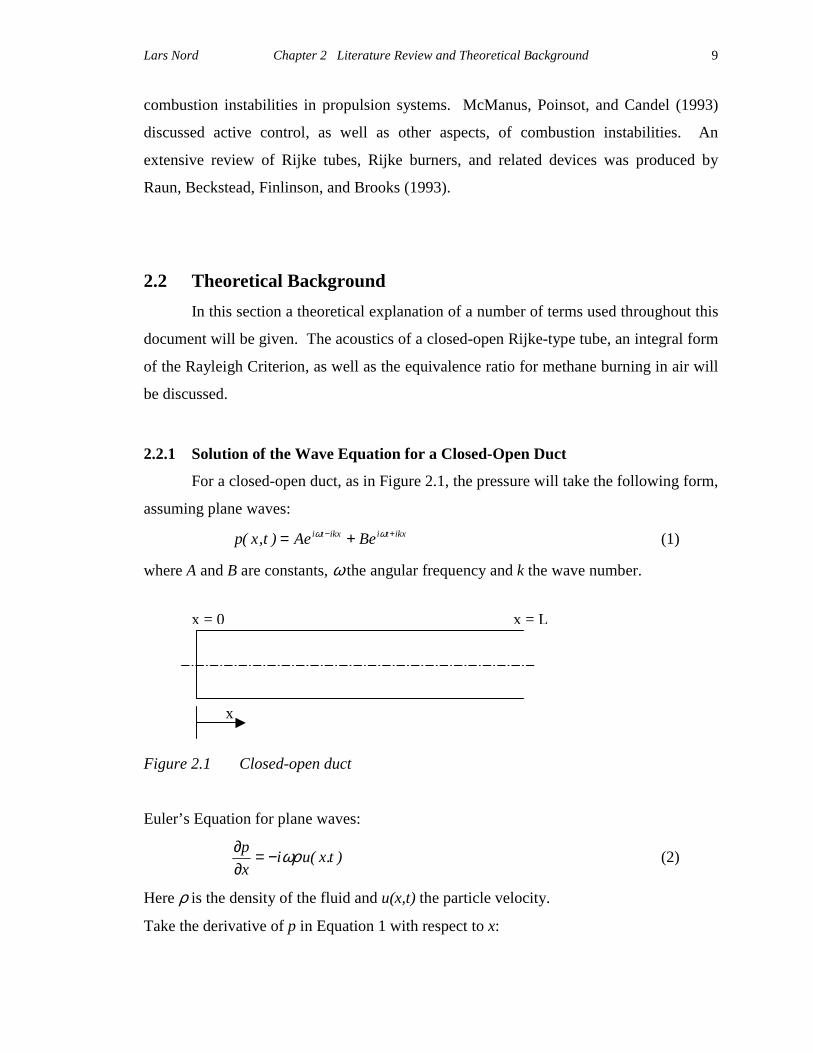
For a closed-open duct, as in Figure 2.1, the pressure will take the following form,
assuming plane waves: ikxtiikxti BeAe)t,x(p +− += ωω (1)
where A and B are constants, ω the angular frequency and k the wave number.
Figure 2.1 Closed-open duct
Euler’s Equation for plane waves:
)t.x(uixp ωρ−=∂∂ (2)
Here ρ is the density of the fluid and u(x,t) the particle velocity.
Take the derivative of p in Equation 1 with respect to x:
x
x = 0 x = L
Lars Nord Chapter 2 Literature Review and Theoretical Background
10
ikxtiikxti ikBeikAexp +− +−=∂∂ ωω (3)
and substitute into Euler’s Equation:
ωρωρ
ωω
iikBe
iikAe)t,x(u
ikxtiikxti
−+=
+−
(4)
Since c
k ω= , where c is the speed of sound in the fluid, the expression can be
simplified:
cBeAe)t,x(u
ikxtiikxti
ρ
ωω +− −= (5)
Boundary condition at x = 0:
0)t,0(u = (6)
This gives:
0cBeAe titi
=−ρ
ωω
(7)
Which gives:
0BA =− (8)
Or:
BA = (9)
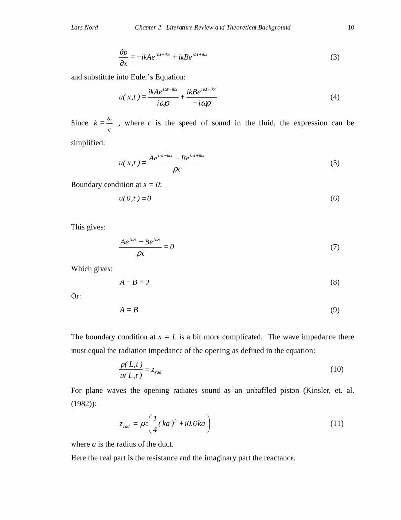
The boundary condition at x = L is a bit more complicated. The wave impedance there
must equal the radiation impedance of the opening as defined in the equation:
radz)t,L(u)t,L(p = (10)
For plane waves the opening radiates sound as an unbaffled piston (Kinsler, et. al.
(1982)):
+= ka6.0i)ka(
41cz 2
rad ρ (11)
where a is the radius of the duct.
Here the real part is the resistance and the imaginary part the reactance.

Lars Nord Chapter 2 Literature Review and Theoretical Background
11
Using Equations (1), (5), and (9), the left-hand side of Equation (10) can be written as:
−+=
+−
+−
cAeAeAeAe
)t,L(u)t,L(p
ikLtiikLti
ikLtiikLti
ρ
ωω
ωω
(12)
Or simplified:
ikLikL
ikLikL
eeeec
)t,L(u)t,L(p
−+= −
−
ρ (13)
Since
)sin(i)cos(ei θθθ += (14)
Equation (13) can be written as:
)kLsin(i)kLcos()kLsin(i)kLcos()kLsin(i)kLcos()kLsin(i)kLcos(c
)t,L(u)t,L(p
−−−+−++−+−= ρ (15)
Since )kLcos()kLcos( =− , and )kLsin()kLsin( −=− Equation (15) can be written as:
)kLsin(i2)kLcos(2c
)t,L(u)t,L(p
−= ρ (16)
Or:
)kLcot(ci)t,L(u)t,L(p ρ= (17)
For resonance, the resistive part of the radiation impedance goes to zero which gives the
following expression:
ka6.0ciz resonance,rad ρ= (18)
Equate Equations (17) and (18):
ka6.0c)kLcot(c ρρ = (19)
Or:
ka6.0)kLcot( = (20)
This equation can be solved numerically, or one can use the fact that for 1ka <<
)ka6.0tan(ka6.0 ≈ (21)
Equation (20) can now be rewritten as:
)ka6.0tan()kLcot( ≈ (22)
Lars Nord Chapter 2 Literature Review and Theoretical Background
12
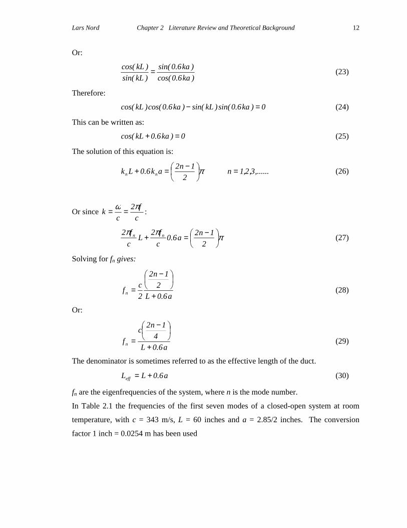
Or:
)ka6.0cos()ka6.0sin(
)kLsin()kLcos( = (23)
Therefore:
0)ka6.0sin()kLsin()ka6.0cos()kLcos( =− (24)
This can be written as:
0)ka6.0kLcos( =+ (25)
The solution of this equation is:
,......3,2,1n2
1n2ak6.0Lk nn =
−=+ π (26)
Or since cf2
ck πω == :
πππ
−=+
21n2a6.0
cf2
Lcf2 nn (27)
Solving for fn gives:
a6.0L2
1n2
2cfn +
−
= (28)
Or:
a6.0L4
1n2cfn +
−
= (29)
The denominator is sometimes referred to as the effective length of the duct.
a6.0LLeff += (30)
fn are the eigenfrequencies of the system, where n is the mode number.
In Table 2.1 the frequencies of the first seven modes of a closed-open system at room
temperature, with c = 343 m/s, L = 60 inches and a = 2.85/2 inches. The conversion
factor 1 inch = 0.0254 m has been used

Lars Nord Chapter 2 Literature Review and Theoretical Background
13
Table 2.1 The 7 first eigenfrequencies of the system
Mode Number n Eigenfrequency fn [Hz] 1 55 2 166 3 277 4 388 5 499 6 610 7 721
2.2.2 The Rayleigh Criterion
Thermoacoustic instabilities are the result of the coupling between the unsteady
heat release and the acoustic pressure, and they are well described by the Rayleigh
Integral:
, where R is the Rayleigh Index, )t(p′ the acoustic pressure and )t(Q′ the unsteady part
of the heat release rate.
The unsteady heat release is proportional to the acoustic particle velocity )( τ−′ tuv , where
τ is the time lag between a change in flow rate and a change in heat release rate:
This leads to the following integral:
Adding heat where the Rayleigh Index is negative would add damping to the system,
whereas adding heat where the Rayleigh Index is positive could lead to thermoacoustic
instability if the amount of heat added is large enough to overcome the damping of the
system. In Figure 2.1 are the spatial distribution of the acoustic pressure, particle
∫+
=Tt
tdt)t(Q')t(p'R
)-t('u~)t('Q τv
∫+
≅Tt
tdt)-t('u)t(p'R τv
Lars Nord Chapter 2 Literature Review and Theoretical Background
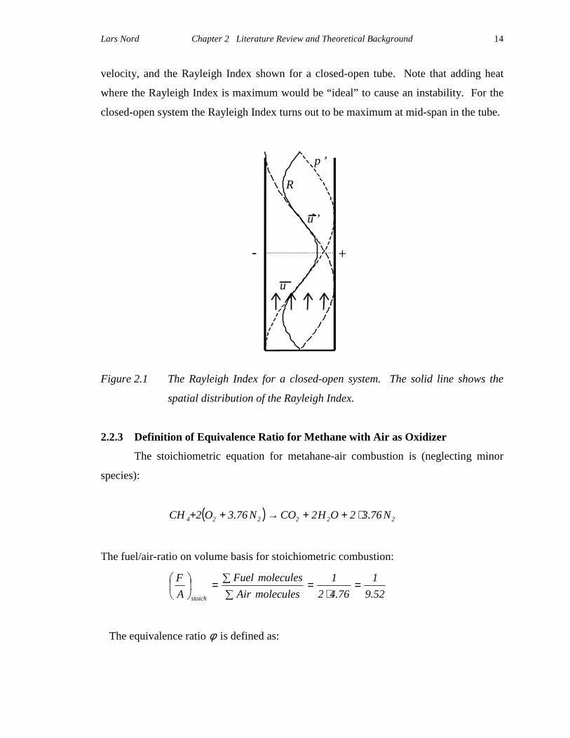
14
velocity, and the Rayleigh Index shown for a closed-open tube. Note that adding heat
where the Rayleigh Index is maximum would be “ideal” to cause an instability. For the
closed-open system the Rayleigh Index turns out to be maximum at mid-span in the tube.
Figure 2.1 The Rayleigh Index for a closed-open system. The solid line shows the
spatial distribution of the Rayleigh Index.
2.2.3 Definition of Equivalence Ratio for Methane with Air as Oxidizer
The stoichiometric equation for metahane-air combustion is (neglecting minor
species):
( ) 222224 N76.32OH2CON76.3O2CH ⋅++→++
The fuel/air-ratio on volume basis for stoichiometric combustion:
52.91
76.421
moleculesAirmoleculesFuel
AF
stoich
=⋅
=∑∑=
The equivalence ratio φ is defined as:
p ’
R
u ’
u
- +
Lars Nord Chapter 2 Literature Review and Theoretical Background
15
air
fuel
actual
stoic
actual
52.9AF52.9
AFAF
=
=
=φ
where Qfuel is the volumetric flow of fuel and Qair is the volumetric flow of air.
The fuel-air ratio on mass basis:
=⋅⋅+⋅
⋅=
∑=
22
4
NO
CH
iii
fuelfuel
stoic MW76.32MW2MW1
MWnMWn
AF
12.171
014.2876.32999.31204.16 =
⋅⋅+⋅=
where ni is the number of moles of species i and MWi the molecular weight of species i.
air
fuel
actual
stoic
actual
mm
12.17AF12.17
AFAF
&
&=
=
=φ
Here fuelm& is the mass flow of fuel and airm& is the mass flow of air.
16
Chapter 3 Experimental Systems and Methods
3.1 Overview of Experimental Components
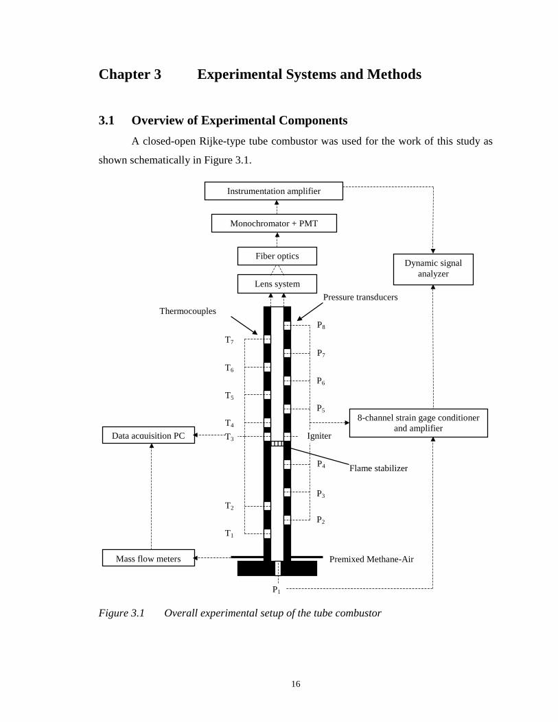
A closed-open Rijke-type tube combustor was used for the work of this study as
shown schematically in Figure 3.1.
Figure 3.1 Overall experimental setup of the tube combustor
Premixed Methane-Air
8-channel strain gage conditioner and amplifier
Pressure transducers Thermocouples
Monochromator + PMT
Flame stabilizer
P1
P3
P2
P5
P6
P7
P8
P4
T1
T2
T3
T4
T7
T6
T5
Igniter
Instrumentation amplifier
Lens system
Data acquisition PC
Dynamic signal analyzer
Fiber optics
Mass flow meters
Lars Nord Chapter 3 Experimental Systems and Methods
17
Premixed methane-air coming from a gas mixer was fed into the bottom part of the
combustor through copper tubes with small holes drilled in the cylindrical shaped tubes.
The flame was stabilized by a ceramic honeycomb, located mid-span, where the Rayleigh
Index is maximum for the 2nd acoustic mode, as mentioned in Chapter 2. For temperature
measurements seven type K thermocouples were inserted through the combustor wall
with the bead located on the centerline of the combustor. The data was processed in a
data acquisition PC. For pressure measurements, pressure transducers were mounted on
the opposite side as well as one in the bottom of the tube and were connected to a strain
gage amplifier and conditioner. The data was processed in a dynamic signal analyzer.
For chemiluminescence measurements of the flame, an optical system was utilized,
which consisted of lenses, a fiber optic cable, a monochromator, and a photomultiplier
tube (PMT). The signal from the PMT was amplified and analyzed with a dynamic
signal analyzer.
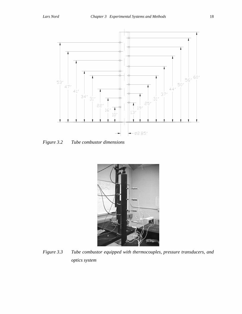
3.2 Tube Combustor
The tube combustor itself consisted of a 60” long steel tube with an inner
diameter of 2.85”, as seen in Figures 3.2 and 3.3. Seven holes, to be used for insertion of
two thermocouples below and five above the flame holder, were drilled and tapped on
one side of the combustor. On the opposite side seven holes for pressure transducers
were drilled and tapped. In addition, an igniter for ignition of the pre-mixed methane-air
was inserted one inch above the flame holder. A hole for a pressure transducer was also
located in the bottom of the tube for use as a reference for the acoustic pressure since a
pressure maximum will always be located at the closed end regardless of the frequency of
the fluctuation. The flame is viewable through two view windows on each side of the
tube. A mount for the optical system was located on top of the combustor.
Lars Nord Chapter 3 Experimental Systems and Methods
18
Figure 3.2 Tube combustor dimensions
Figure 3.3 Tube combustor equipped with thermocouples, pressure transducers, and
optics system

Lars Nord Chapter 3 Experimental Systems and Methods
19
The ceramic honeycomb [Al2O3] used for the stabilization of the laminar flame in
the combustor is shown in Figure 3.4. The flame stabilizer was mounted 30” from the
bottom of the tube combustor for excitation of the 2nd acoustic mode.
Figure 3.4 Ceramic honeycomb used as a flame holder in the tube combustor. The
area restriction was approximately 50%.
3.3 Pressure Transducers
The pressure transducers, Sensym low-pressure transducers, were mounted in T-
connections as shown in Figure 3.5. One of the connections in the T was connected to
the tube combustor via a teflon connector. The opposite connection was connected to an
“infinite tube”, a five meters long plastic tube, to limit the reflective pressure waves
travelling back up the line and affecting the pressure at the transducer. The third
connection was used for calibration of the transducers. The calibration procedure is
described in a technical brief by Richards, et. al. (1999). The signals from the eight
pressure transducers were amplified in a strain gage conditioner and amplifier, model
2100, made by Measurements Group Incorporated.
In the pressure measurements, the effects of errors in the strain gage conditioner
and amplifier as well as in the Hewlett Packard dynamic signal analyzer were negligible
compared to the error in the transducer itself. The error for the Sensym pressure
transducers were within ± 0.2 %.

Lars Nord Chapter 3 Experimental Systems and Methods
20
Figure 3.5 Sensym pressure transducer mounted in a T-connection
3.4 Thermocouples
The temperature measurements were conducted with thermocouples of type K, as
seen in Figure 3.6. The wire used was 0.01” diameter type K thermocouple wire. The
bead diameter ranged from 0.029” to 0.04” for the thermocouples. The measured surface
temperature of the thermocouple may be considerable different from the desired gas
temperature. With the bead diameter being approximately three to four times larger than
the lead wire, the convective behavior of the bead is close to that of a cylinder [Hibshman
(1999)]. The analysis described by Hibshman was initially used to correct the
temperatures; however, findings by one of the VACCG members, Vivek Khanna,
suggested that due to interaction between the walls, the honeycomb, and the
thermocouple beads, a different approach was necessary. The findings arose at the end of
the author’s research at Virginia Tech and will not be discussed in this thesis;
consequently, the collected temperature data was left uncorrected.
The fabrication procedure of the thermocouples and the data acquisition system
for collection of the temperature data are described in a technical brief by Grove, et. al.
(1999).
The error in the temperature measurements mainly came from the thermocouples.
ASTM standards specify that the initial calibration tolerances for type K thermocouples
be ± 2.2°C or ± 0.75 %, whichever is greater, for the temperature range 0°C to 1250°C.

Lars Nord Chapter 3 Experimental Systems and Methods
21
The maximum error in the 8th-order polynomials describing the temperature as a function
of voltage is ± 0.7°C for the temperature range 0°C to 1370°C.
Figure 3.6 Type K thermocouple
3.5 Optical System for Chemiluminescence Measurements
To measure the heat release oscillation of the flame in the tube combustor an
optical system was utilized. Excited OH-radicals, which when going from their excited
state to their ground state emit light, are assumed to be proportional to the heat release
rate from the flame. The optical system used for these chemiluminescence measurements
consisted of the following:
- A system of two short focal length lenses: Two, 25.4 mm fused silica lenses.
- Optical Fiber: 200 µm, silica core fiber.
- Monochromator: 0.5 m Jarrell-Ash monochromator.
- Photomultiplier: R955 Hamamatsu ten stages photomultiplier tube.
The setup, constructed by VACCG member Ludwig Haber, is shown in Figure 3.7.
Lars Nord Chapter 3 Experimental Systems and Methods
22
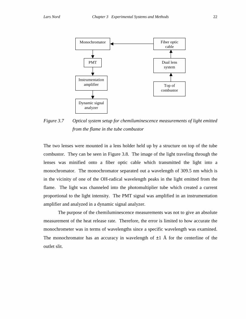
Figure 3.7 Optical system setup for chemiluminescence measurements of light emitted
from the flame in the tube combustor
The two lenses were mounted in a lens holder held up by a structure on top of the tube
combustor. They can be seen in Figure 3.8. The image of the light traveling through the
lenses was minified onto a fiber optic cable which transmitted the light into a
monochromator. The monochromator separated out a wavelength of 309.5 nm which is
in the vicinity of one of the OH-radical wavelength peaks in the light emitted from the
flame. The light was channeled into the photomultiplier tube which created a current
proportional to the light intensity. The PMT signal was amplified in an instrumentation
amplifier and analyzed in a dynamic signal analyzer.
The purpose of the chemiluminescence measurements was not to give an absolute
measurement of the heat release rate. Therefore, the error is limited to how accurate the
monochrometer was in terms of wavelengths since a specific wavelength was examined.
The monochromator has an accuracy in wavelength of ±1 Å for the centerline of the
outlet slit.
Fiber optic cable
Dual lens system
Monochromator
Top of combustor
PMT
Instrumentation amplifier
Dynamic signal analyzer

Lars Nord Chapter 3 Experimental Systems and Methods
23
Figure 3.8 Lenses and fiber optics setup on top of the tube combustor
3.6 Mass Flow Meters
Two Hastings Instruments HFM-200 mass flow meters, one for the air and the
other for the methane, were utilized for measuring the incoming mass flows to the fuel-
air mixer upstream of the tube combustor.
Air mass flow meter range: 0-25.000 Standard liters/minute.
Methane mass flow meter range: 0-1.5000 Standard liters/minute.
The accuracy specifications for the two mass flow meters were 1 % of full scale.
With full scales as mentioned above, the accuracy would be ±0.25 Standard liters/minute
and ±0.015 Standard liters/minute respectively. A drift in the zero setting of the air mass
flow meter also occurred where the maximum drift caused an error of +0.25 Standard
liters/minute. The standard state is defined as 0°C, and 760 torr.

Lars Nord Chapter 3 Experimental Systems and Methods
24
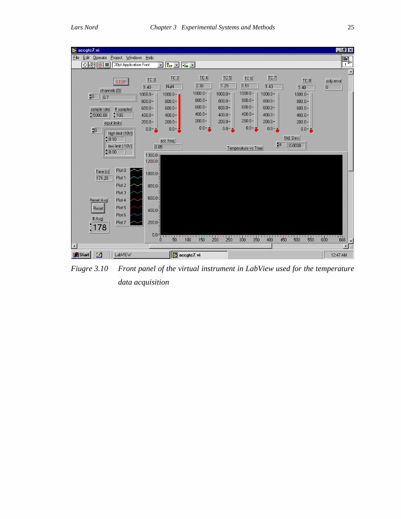
3.7 Data Acquisition Equipment
Two data acquisition boards mounted in a PC Pentium 200 were used to acquire
the fuel and air mass flows as well as the temperature data. The software utilized was
LabView version 4 by National Instruments. Screen shots of the virtual instruments used
in LabView are shown in Figures 3.9 and 3.10. The data acquisition boards used were
DT2801-A for flow measurements and DT2805 for temperature measurements. Pressure
measurement as well as chemiluminescence measurements were analyzed with a Hewlett
Packard dynamic signal analyzer 35665A .
Fiugre 3.9 Front panel of the virtual instrument in LabView used for the flow data
acquisition
Lars Nord Chapter 3 Experimental Systems and Methods
25
Fiugre 3.10 Front panel of the virtual instrument in LabView used for the temperature
data acquisition
26
Chapter 4 Rijke-tube Thermoacoustic Characterization
VACCG members have investigated a number of theories associated with the
phenomena occurring in the tube combustor. The research presented in this chapter will,
with the help of extensive experimental data, strengthen the suggested theories. The
experiments conducted also serves as a database for the VACCG and the research
community within this field. In addition the collected data can be helpful in the
development of reduced-order modeling schemes that provide adequate prediction
capabilities for the occurrence of thermoacoustic instabilities. The experimental
investigation included a mapping of the tube combustor in terms of acoustic pressure,
temperature distribution, and chemiluminescence for the whole operating range.
Different regions in the pressure power spectrum and in the OH*-spectrum (OH-radicals
assumed proportional to the unsteady heat release rate) are analyzed, and the analysis
includes a discussion of two different types of flame instabilities, namely pulsating and
vibrating flames. In addition, temperature profiles and tube resonances are presented.
4.1 Acoustic Pressure
The signature of the acoustic pressure exhibits useful information of the system
and it can help to identify reduced-order schemes that provide adequate prediction
capabilities for the occurrence and control of thermoacoustic instabilities. A typical
pressure spectrum of the tube combustor can be seen in Figure 4.1, where the pressure is
measured with the pressure transducer located at the closed end of the combustor.
Lars Nord Chapter 4 Rijke-tube Thermoacoustic Characterization
27
0 100 200 300 400 500 600 700 800
40
60
80
100
120
140
160
Frequency [Hz]
SP
L [d
B],
ref
2e-
5 P
a
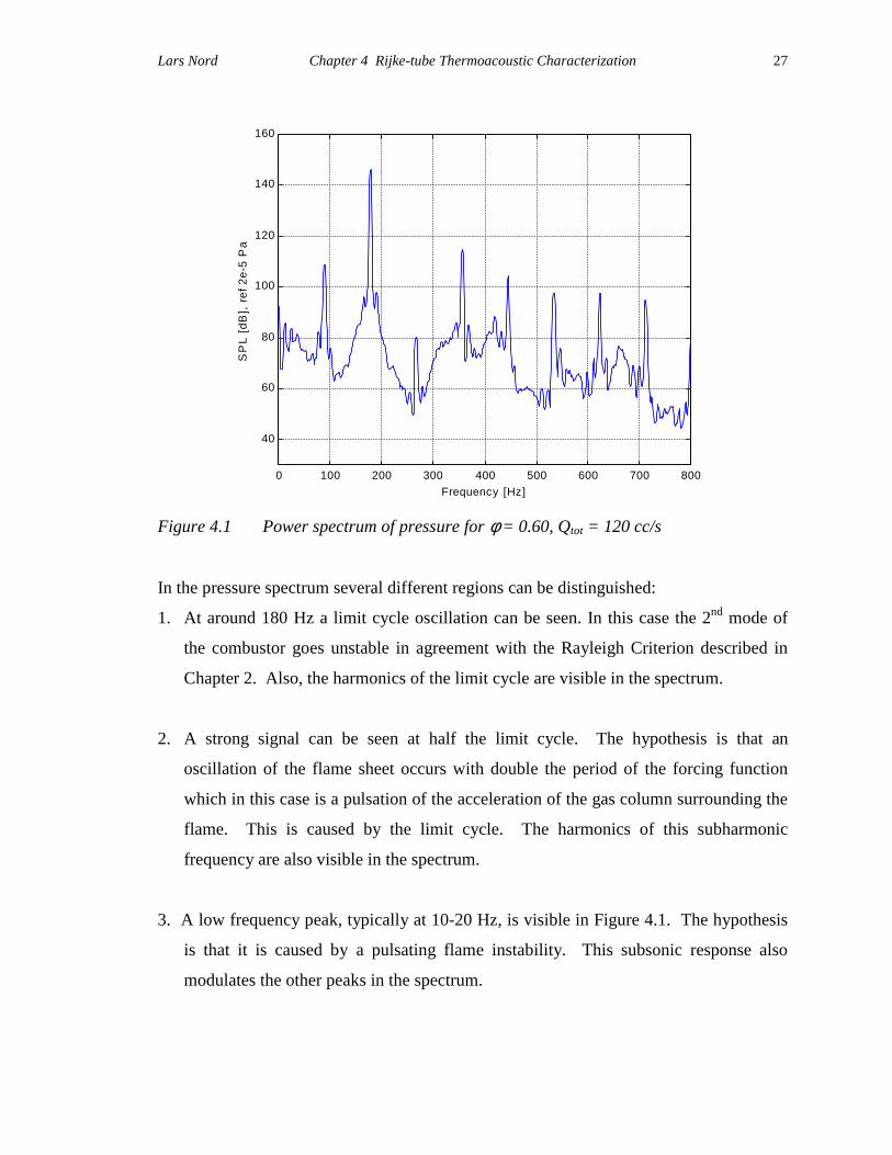
Figure 4.1 Power spectrum of pressure for φ = 0.60, Qtot = 120 cc/s
In the pressure spectrum several different regions can be distinguished:
1. At around 180 Hz a limit cycle oscillation can be seen. In this case the 2nd mode of
the combustor goes unstable in agreement with the Rayleigh Criterion described in
Chapter 2. Also, the harmonics of the limit cycle are visible in the spectrum.
2. A strong signal can be seen at half the limit cycle. The hypothesis is that an
oscillation of the flame sheet occurs with double the period of the forcing function
which in this case is a pulsation of the acceleration of the gas column surrounding the
flame. This is caused by the limit cycle. The harmonics of this subharmonic
frequency are also visible in the spectrum.
3. A low frequency peak, typically at 10-20 Hz, is visible in Figure 4.1. The hypothesis
is that it is caused by a pulsating flame instability. This subsonic response also
modulates the other peaks in the spectrum.
Lars Nord Chapter 4 Rijke-tube Thermoacoustic Characterization
28
In the following text these different features will either be explained, or at least a
hypothesis presented for the origin of these characteristics.
4.1.1 Limit Cycle and Harmonics
In certain non-linear systems a self-excited oscillation, or a limit cycle occurs.
Consider, for example, the following mass-spring-damper system:
0kxx)x1(cxm 2 =+−− &&&
where m is the mass, c(1-x2) the damping term, and k the stiffness term of the system.
For small values of x the damping will be negative and will put energy in to the system,
but for large values of x the damping will be positive and remove energy from the
system. At some displacement amplitude x of the system, the system will reach a limit
cycle due to this damping term.
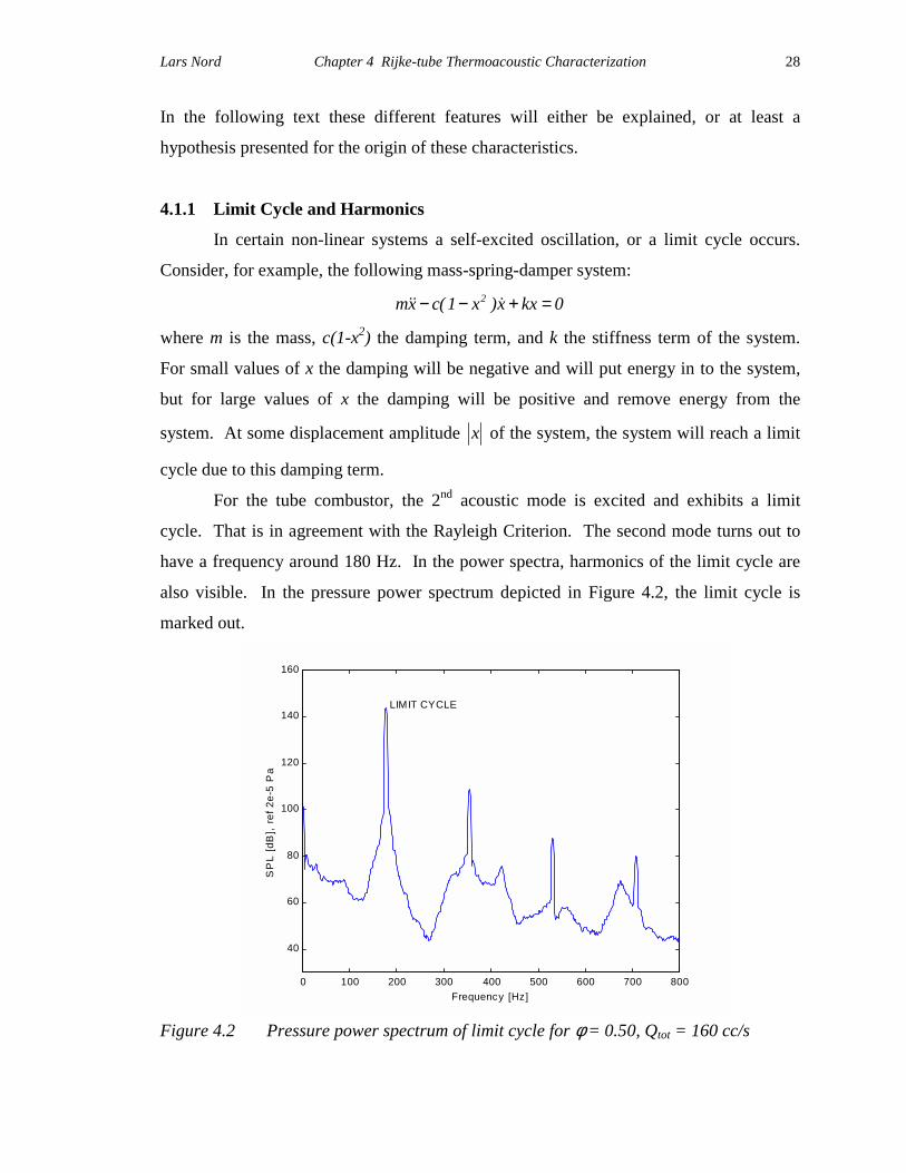
For the tube combustor, the 2nd acoustic mode is excited and exhibits a limit
cycle. That is in agreement with the Rayleigh Criterion. The second mode turns out to
have a frequency around 180 Hz. In the power spectra, harmonics of the limit cycle are
also visible. In the pressure power spectrum depicted in Figure 4.2, the limit cycle is
marked out.
0 100 200 300 400 500 600 700 800
40
60
80
100
120
140
160
Frequency [Hz]
SP
L [d
B],
ref
2e-
5 P
a
LIMIT CYCLE
Figure 4.2 Pressure power spectrum of limit cycle for φ = 0.50, Qtot = 160 cc/s
Lars Nord Chapter 4 Rijke-tube Thermoacoustic Characterization
29
4.1.2 Subharmonic Response
The hypothesis, described by Markstein (1964), assumes that the flame can be
approximated as a membrane which exhibits oscillations. Markstein treated the flame as
a membrane, and forced it with an oscillation of the acceleration of the gas column
surrounding the flame. The differential equation that describes this situation is based on
non-linear second-order dynamics:
0F)]1)(1(2[F)1(2F)1( 411
44 =−−++′++′′− −− γκεκκε (31)
with F4 being the amplitude of the flame distortion, burned
unburned
ρρε = , κ a dimensionless
wave number KL=κ , where K is the wave number and L a characteristic length. γ is a
dimensionless acceleration )t(aSL)(
uετγ = . Here Su is the laminar flame speed and a(t)
the variable acceleration.
When the following substitutions are made in Equation 31:
uSK2t
21z
εωτω ==
4z F)z(Ye ′=−β
where )1( += κΩκβ , with
u
1
SL)1(
21 ωεΩ −+=
the standard form of the Mathieu’s equation results:
0Y)z2cosq2a(Y =−+′′ (32)
where )12()(a 122 −−+−= − εεκεκΩκ and Dq κ= . Here
Ld
112D+−=εε .
The solution of the Mathieu’s equation can be written as:
)z(eC)z(eC)z(Y z2
z1 −+= − ΦΦ µµ (33)
where C1 and C2 are arbitrary constants and )z(Φ is either of double the period of the
forcing function or of the same period as the forcing function. Here thL
L=µ , where Lth
Lars Nord Chapter 4 Rijke-tube Thermoacoustic Characterization
30
is the thermal width of the flame front uup
th SckLρ
= , with k being the thermal
conductivity and cp the specific heat at constant pressure.
The solution dependence on the values of µ and )z(Φ leads to either a stable or
unstable solution. If unstable, the function )z(Φ will have either the same period as the
forcing or double the period. In the case of the flame in the tube combustor, the solution
ends up unstable in the region where the period has twice the period of the forcing. The
forcing in this case is, as mentioned before, the pulsation of the acceleration of the gas
column determined by the thermoacoustic limit cycle response. Double the period
corresponds to half the frequency, which means the flame sheet would oscillate with a
frequency half of the limit cycle frequency. When the flame sheet oscillates, the flame
surface area changes, and since the heat release is proportional to the flame surface area
the heat release rate will oscillate. In addition, as the flame oscillates, the heat loss to the
flame stabilizer and the combustor walls changes which leads to a change in the net heat
put into the gas. The change in heat release couples with the acoustic particle velocity
and one can expect to see a subharmonic peak at half the limit cycle frequency in the
pressure spectra as well as in the chemiluminescence spectra at a frequency around 90
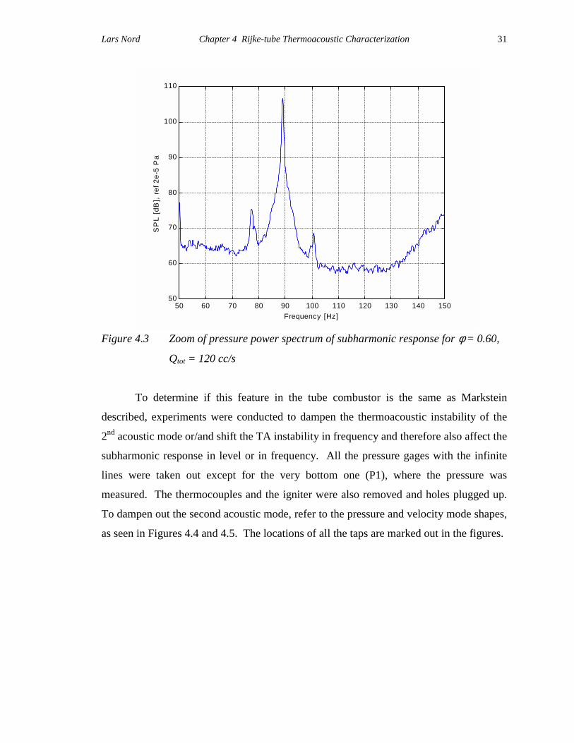
Hz. A zoom around the subharmonic response can be seen in Figure 4.3.
Lars Nord Chapter 4 Rijke-tube Thermoacoustic Characterization
31
50 60 70 80 90 100 110 120 130 140 15050
60
70
80
90
100
110
Frequency [Hz]
SP
L [d
B],
ref
2e-
5 P
a
Figure 4.3 Zoom of pressure power spectrum of subharmonic response for φ = 0.60,
Qtot = 120 cc/s
To determine if this feature in the tube combustor is the same as Markstein
described, experiments were conducted to dampen the thermoacoustic instability of the
2nd acoustic mode or/and shift the TA instability in frequency and therefore also affect the
subharmonic response in level or in frequency. All the pressure gages with the infinite
lines were taken out except for the very bottom one (P1), where the pressure was
measured. The thermocouples and the igniter were also removed and holes plugged up.
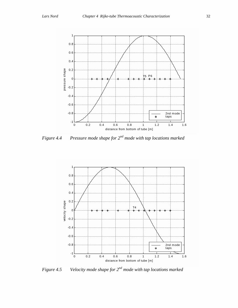
To dampen out the second acoustic mode, refer to the pressure and velocity mode shapes,
as seen in Figures 4.4 and 4.5. The locations of all the taps are marked out in the figures.
Lars Nord Chapter 4 Rijke-tube Thermoacoustic Characterization
32
0 0.2 0.4 0.6 0.8 1 1.2 1.4 1.6-1
-0.8
-0.6
-0.4
-0.2
0
0.2
0.4
0.6
0.8
1
distance from bottom of tube [m]
pres
sure
sha
pe
T5 P6
2nd modetaps
Figure 4.4 Pressure mode shape for 2nd mode with tap locations marked
0 0.2 0.4 0.6 0.8 1 1.2 1.4 1.6-1
-0.8
-0.6
-0.4
-0.2
0
0.2
0.4
0.6
0.8
1
distance from bottom of tube [m]
velo
city
sha
pe
T4
2nd modetaps
Figure 4.5 Velocity mode shape for 2nd mode with tap locations marked
Lars Nord Chapter 4 Rijke-tube Thermoacoustic Characterization
33
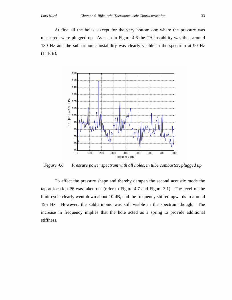
At first all the holes, except for the very bottom one where the pressure was
measured, were plugged up. As seen in Figure 4.6 the TA instability was then around
180 Hz and the subharmonic instability was clearly visible in the spectrum at 90 Hz
(111dB).
0 100 200 300 400 500 600 700 80050
60
70
80
90
100
110
120
130
140
150
160
Frequency [Hz]
SP
L [d
B],
ref
2e-
5 P
a
Figure 4.6 Pressure power spectrum with all holes, in tube combustor, plugged up
To affect the pressure shape and thereby dampen the second acoustic mode the
tap at location P6 was taken out (refer to Figure 4.7 and Figure 3.1). The level of the
limit cycle clearly went down about 10 dB, and the frequency shifted upwards to around
195 Hz. However, the subharmonic was still visible in the spectrum though. The
increase in frequency implies that the hole acted as a spring to provide additional
stiffness.
Lars Nord Chapter 4 Rijke-tube Thermoacoustic Characterization
34
0 100 200 300 400 500 600 700 80050
60
70
80
90
100
110
120
130
140
150
160
Frequency [Hz]
SP
L [d
B],
ref
2e-
5 P
a
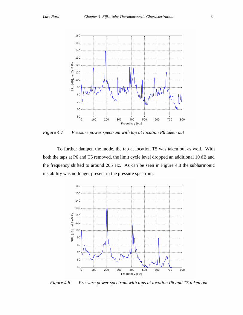
Figure 4.7 Pressure power spectrum with tap at location P6 taken out
To further dampen the mode, the tap at location T5 was taken out as well. With
both the taps at P6 and T5 removed, the limit cycle level dropped an additional 10 dB and
the frequency shifted to around 205 Hz. As can be seen in Figure 4.8 the subharmonic
instability was no longer present in the pressure spectrum.
0 100 200 300 400 500 600 700 80050
60
70
80
90
100
110
120
130
140
150
160
Frequency [Hz]
SP
L [d
B],
ref
2e-
5 P
a
Figure 4.8 Pressure power spectrum with taps at location P6 and T5 taken out
Lars Nord Chapter 4 Rijke-tube Thermoacoustic Characterization
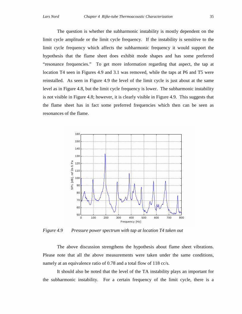
35
The question is whether the subharmonic instability is mostly dependent on the
limit cycle amplitude or the limit cycle frequency. If the instability is sensitive to the
limit cycle frequency which affects the subharmonic frequency it would support the
hypothesis that the flame sheet does exhibit mode shapes and has some preferred
“resonance frequencies.” To get more information regarding that aspect, the tap at
location T4 seen in Figures 4.9 and 3.1 was removed, while the taps at P6 and T5 were
reinstalled. As seen in Figure 4.9 the level of the limit cycle is just about at the same
level as in Figure 4.8, but the limit cycle frequency is lower. The subharmonic instability
is not visible in Figure 4.8; however, it is clearly visible in Figure 4.9. This suggests that
the flame sheet has in fact some preferred frequencies which then can be seen as
resonances of the flame.
0 100 200 300 400 500 600 700 80050
60
70
80
90
100
110
120
130
140
150
160
Frequency [Hz]
SP
L [d
B],
ref
2e-
5 P
a
Figure 4.9 Pressure power spectrum with tap at location T4 taken out
The above discussion strengthens the hypothesis about flame sheet vibrations.
Please note that all the above measurements were taken under the same conditions,
namely at an equivalence ratio of 0.78 and a total flow of 118 cc/s.
It should also be noted that the level of the TA instability plays an important for
the subharmonic instability. For a certain frequency of the limit cycle, there is a

Lars Nord Chapter 4 Rijke-tube Thermoacoustic Characterization
36
‘threshold’ amplitude that the limit cycle must have to drive the subharmonic instability.
The threshold amplitude changes in level depending on the frequency of the limit cycle,
as discussed previously, where it was stated that the flame sheet seems to have some
preferred frequencies.
Still, further proof of the existence of a vibrating flame is necessary. For this
purpose, a bench-top burner was constructed to study the possibility of a flame sheet
exhibiting mode shapes. The experimental setup, constructed by VACCG member Chris
A. Fannin, is shown schematically in Figure 4.10. A speaker connected to a plenum with
an injection port for reactants, in this case premixed methane-air, and a port for pressure
measurements, was used. On the top of the plenum, a ceramic honeycomb was placed to
stabilize the flame. Phase locked photographs with a CCD camera were taken of the
flame sheet.
Figure 4.10 Bench-top burner for the study of flame sheet mode shapes
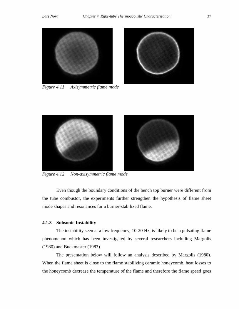
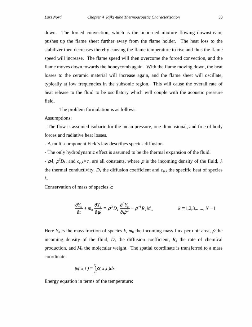
CCD camera images of two flame modes are shown in Figures 4.11 and 4.12. The lighter
areas indicate higher flame intensity. The axisymmetric mode in Figure 4.11 shifted
between being dark in the center and light in the center. The non-axisymmetric mode in
Figure 4.12 shifted between one half lit up/one half dark and then reversed.
Injection of premixed methane-air
Pressure transducer
Speaker
Plenum
Ceramic honeycomb
Lars Nord Chapter 4 Rijke-tube Thermoacoustic Characterization
37
Figure 4.11 Axisymmetric flame mode
Figure 4.12 Non-axisymmetric flame mode
Even though the boundary conditions of the bench top burner were different from
the tube combustor, the experiments further strengthen the hypothesis of flame sheet
mode shapes and resonances for a burner-stabilized flame.
4.1.3 Subsonic Instability
The instability seen at a low frequency, 10-20 Hz, is likely to be a pulsating flame
phenomenon which has been investigated by several researchers including Margolis
(1980) and Buckmaster (1983).
The presentation below will follow an analysis described by Margolis (1980).
When the flame sheet is close to the flame stabilizing ceramic honeycomb, heat losses to
the honeycomb decrease the temperature of the flame and therefore the flame speed goes
Lars Nord Chapter 4 Rijke-tube Thermoacoustic Characterization
38
down. The forced convection, which is the unburned mixture flowing downstream,
pushes up the flame sheet further away from the flame holder. The heat loss to the
stabilizer then decreases thereby causing the flame temperature to rise and thus the flame
speed will increase. The flame speed will then overcome the forced convection, and the
flame moves down towards the honeycomb again. With the flame moving down, the heat
losses to the ceramic material will increase again, and the flame sheet will oscillate,
typically at low frequencies in the subsonic region. This will cause the overall rate of
heat release to the fluid to be oscillatory which will couple with the acoustic pressure
field.
The problem formulation is as follows:
Assumptions:
- The flow is assumed isobaric for the mean pressure, one-dimensional, and free of body
forces and radiative heat losses.
- A multi-component Fick’s law describes species diffusion.
- The only hydrodynamic effect is assumed to be the thermal expansion of the fluid.
- ρλ, ρ2Dk, and cp,k=cp are all constants, where ρ is the incoming density of the fluid, λ
the thermal conductivity, Dk the diffusion coefficient and cp,k the specific heat of species
k.
Conservation of mass of species k:
1,......,3,2,112
22
0 −=−∂∂
=∂∂
+∂∂ − NkMRYDYm
tY
kkk
kkk ρ
ψρ
ψ
Here Yk is the mass fraction of species k, m0 the incoming mass flux per unit area, ρ the
incoming density of the fluid, Dk the diffusion coefficient, Rk the rate of chemical
production, and Mk the molecular weight. The spatial coordinate is transferred to a mass
coordinate:
∫=x
0xd)t,x()t,x( ρψ
Energy equation in terms of the temperature:
Lars Nord Chapter 4 Rijke-tube Thermoacoustic Characterization
39
∑ −+∂∂=
∂∂+
∂∂ −
=
− 1N
1k
0n
0kkk
1p2
2
p0 )hh(MR)c(T
cTm
tT ρ
ψρλ
ψ
Here T is the temperature of the fluid and 0kh the enthalpy of formation for species k.
With the appropriate initial conditions and the boundary conditions stated below for the
two differential equations, the problem is specified.
uT)t,0(T ==ψ
1N,......,3,2,1kYm
DY k0
k
0
k2
k −==∂∂
−=
εψ
ρ
ψ
∞=− ψatboundedY,.....,Y,T 1N1
Here εk is the mass fraction of species k before combustion. For an analysis of the above
stated problem, refer to Margolis (1980). His results show that a steady-state adiabatic
flame is likely to be stable for typical parameter values. However, for incoming flow
velocities sufficiently less than the adiabatic flame speed, the unstable region in his
solution becomes feasible for many flames.
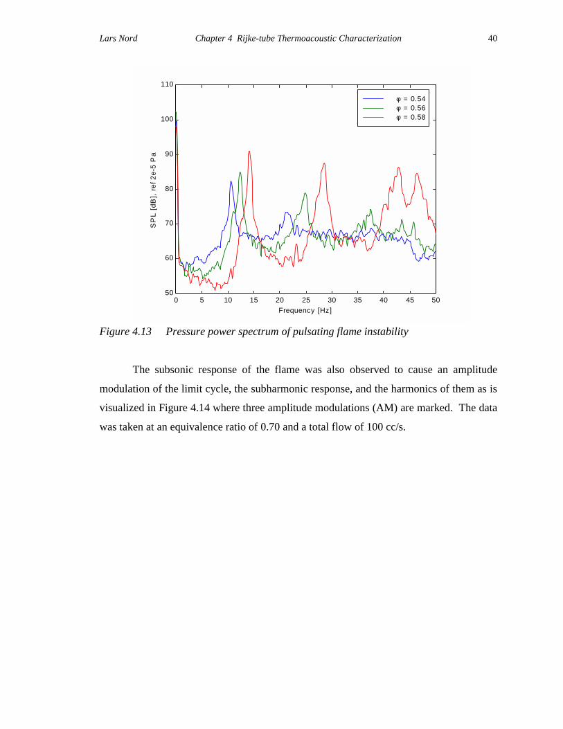
In the tube combustor the frequencies for this pulsating flame instability typically
ranges from 10 to 20 Hz. A tendency of an increase in amplitude and frequency is visible
for an increase in equivalence ratio. Shown in Figure 4.13 is a “zoom” on the frequency
range around the pulsating instability and the tendency of the pulsating frequency to
increase with equivalence ratio can be seen.
Lars Nord Chapter 4 Rijke-tube Thermoacoustic Characterization
40
0 5 10 15 20 25 30 35 40 45 5050
60
70
80
90
100
110
Frequency [Hz]
SP
L [d
B],
ref
2e-
5 P
a
φ = 0.54φ = 0.56φ = 0.58
Figure 4.13 Pressure power spectrum of pulsating flame instability
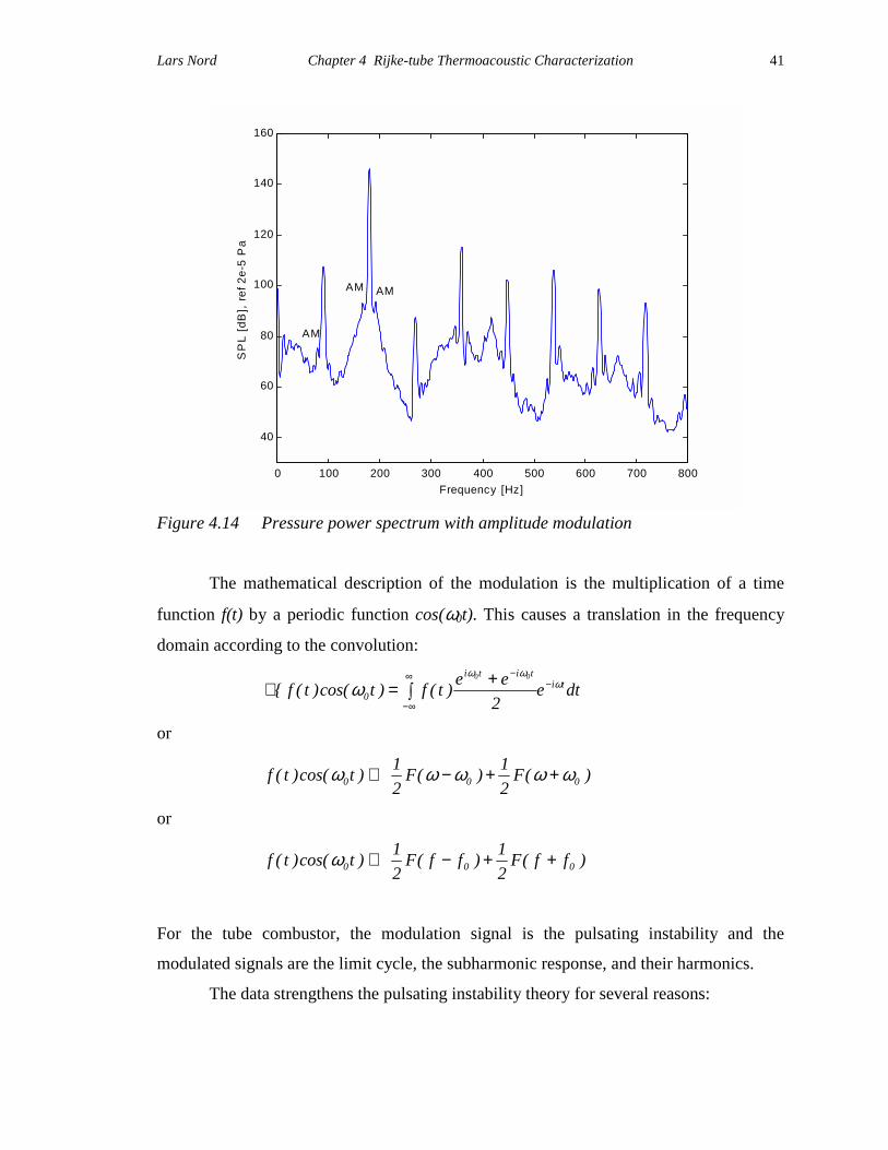
The subsonic response of the flame was also observed to cause an amplitude
modulation of the limit cycle, the subharmonic response, and the harmonics of them as is
visualized in Figure 4.14 where three amplitude modulations (AM) are marked. The data
was taken at an equivalence ratio of 0.70 and a total flow of 100 cc/s.
Lars Nord Chapter 4 Rijke-tube Thermoacoustic Characterization
41
0 100 200 300 400 500 600 700 800
40
60
80
100
120
140
160
Frequency [Hz]
SP
L [d
B],
ref
2e-
5 P
a
AM AM
AM
Figure 4.14 Pressure power spectrum with amplitude modulation
The mathematical description of the modulation is the multiplication of a time
function f(t) by a periodic function cos(ω0t). This causes a translation in the frequency
domain according to the convolution:
dte2
ee)t(f)tcos()t(f tititi
0
00ω
ωω
ω −∞
∞−
−
∫+=ℑ
or
)(F21)(F
21)tcos()t(f 000 ωωωωω ++−⇔
or
)ff(F21)ff(F
21)tcos()t(f 000 ++−⇔ω
For the tube combustor, the modulation signal is the pulsating instability and the
modulated signals are the limit cycle, the subharmonic response, and their harmonics.
The data strengthens the pulsating instability theory for several reasons:
Lars Nord Chapter 4 Rijke-tube Thermoacoustic Characterization
42
- The frequency range observed in the tube combustor is in the same range as described
in the theory.
- The increase in equivalence ratio increases the frequency of the instability in the tube
combustor. This is also suggested in Margolis theory since an increase in the
equivalence ratio increases the flame temperature which, in turn, means higher flame
speed. The higher flame speed would overcome the forced convection quicker and
thus the frequency would increase.
4.2 Chemiluminescence Measurements
The optical system, described in Chapter 3, detects light emitted from the flame.
Radicals that get excited by the chemical reaction emit light when moving from their
excited energy state to their ground state. In the present study, light at a wavelength of
309.5 nm, which is in the vicinity of one of the peaks for the light emitted from excited
OH-molecules, was acquired. The lens system minified the flame image onto the optical
fiber which then channeled the light into the monochromator. The monochromator
separated the wavelengths onto a photomultiplier which yielded a current proportional to
the light intensity and was transferred to an instrumentation amplifier.
However, there were some difficulties related to these measurements. The noise
level sometimes buried some of the peaks in the spectra. The noise was due to the
randomness in the chemical reaction, the dark noise of the PMT, obstruction of the lens
view (thermocouples blocking the light emitted from the flame), and other possible
effects. The signal to noise ratio was improved with the removal of the thermocouples
that blocked some of the light emitted from the flame and with the increase in aperture of
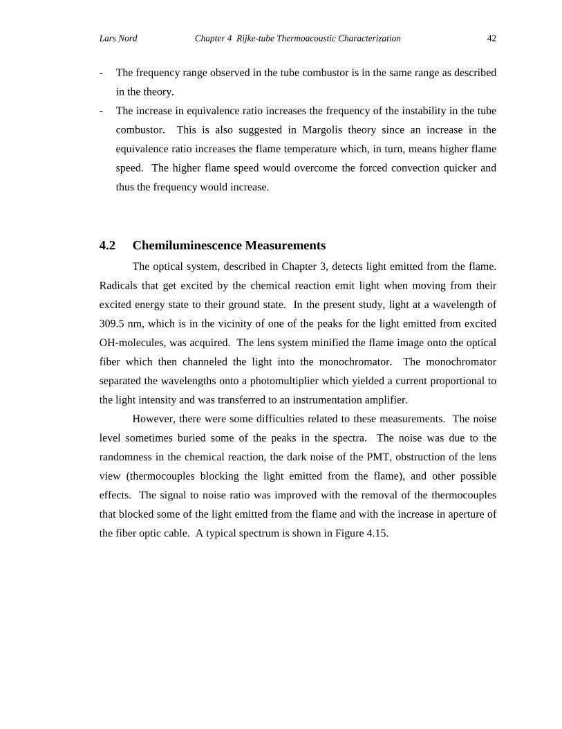
the fiber optic cable. A typical spectrum is shown in Figure 4.15.
Lars Nord Chapter 4 Rijke-tube Thermoacoustic Characterization
43
0 100 200 300 400 500 600 700 800-55
-50
-45
-40
-35
-30
Frequency [Hz]
dBV
rms2 ,
ref 1
Vrm
s
Figure 4.15 Power spectrum of the PMT signal for φ = 0.60, Q = 120 cc/s
Refer to Section 4.6 for further analysis of the chemiluminescence data.
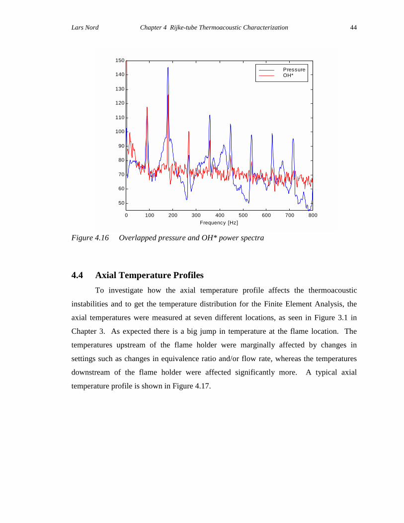
4.3 Comparison of Pressure and Chemiluminescence Spectra
To compare the OH* spectrum with the pressure spectrum, the two spectra are
shown in the same graph in Figure 4.16. The pressure power spectrum and the
chemiluminescence power spectrum are very similar. The peaks of the spectra are
virtually at the same frequencies with the exception that some peaks of the OH* spectrum
get buried in the noise, as mentioned in Section 4.2. The pulsating instability and
oscillating flame sheet phenomena are generally more visible in the chemiluminescence
spectrum. This makes sense since both these phenomena directly affect the heat release
rate from the flame sheet.
Lars Nord Chapter 4 Rijke-tube Thermoacoustic Characterization
44
0 100 200 300 400 500 600 700 800
50
60
70
80
90
100
110
120
130
140
150
Frequency [Hz]
PressureOH*
Figure 4.16 Overlapped pressure and OH* power spectra
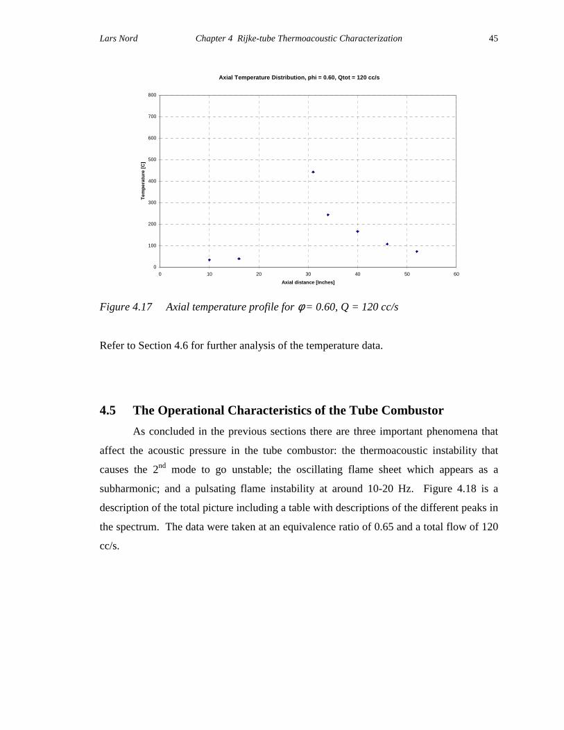
4.4 Axial Temperature Profiles
To investigate how the axial temperature profile affects the thermoacoustic
instabilities and to get the temperature distribution for the Finite Element Analysis, the
axial temperatures were measured at seven different locations, as seen in Figure 3.1 in
Chapter 3. As expected there is a big jump in temperature at the flame location. The
temperatures upstream of the flame holder were marginally affected by changes in
settings such as changes in equivalence ratio and/or flow rate, whereas the temperatures
downstream of the flame holder were affected significantly more. A typical axial
temperature profile is shown in Figure 4.17.
Lars Nord Chapter 4 Rijke-tube Thermoacoustic Characterization
45
Axial Temperature Distribution, phi = 0.60, Qtot = 120 cc/s
0
100
200
300
400
500
600
700
800
0 10 20 30 40 50 60Axial distance [Inches]
Tem
pera
ture
[C]
Figure 4.17 Axial temperature profile for φ = 0.60, Q = 120 cc/s
Refer to Section 4.6 for further analysis of the temperature data.
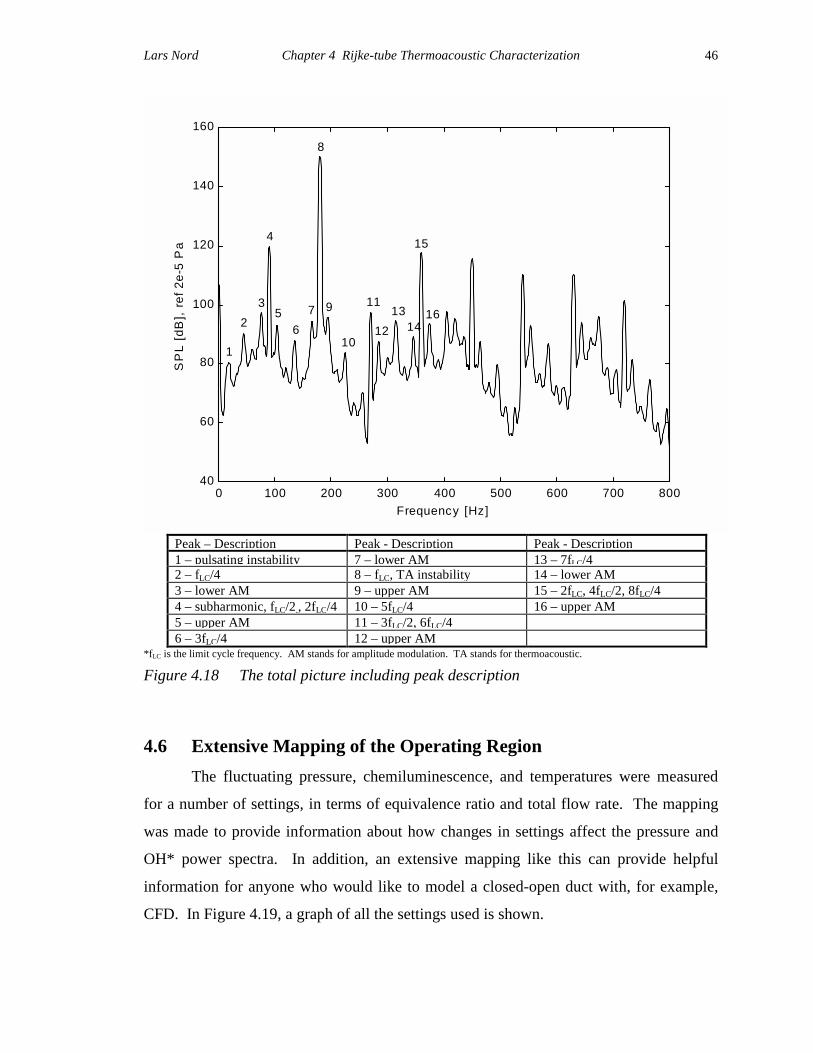
4.5 The Operational Characteristics of the Tube Combustor
As concluded in the previous sections there are three important phenomena that
affect the acoustic pressure in the tube combustor: the thermoacoustic instability that
causes the 2nd mode to go unstable; the oscillating flame sheet which appears as a
subharmonic; and a pulsating flame instability at around 10-20 Hz. Figure 4.18 is a
description of the total picture including a table with descriptions of the different peaks in
the spectrum. The data were taken at an equivalence ratio of 0.65 and a total flow of 120
cc/s.
Lars Nord Chapter 4 Rijke-tube Thermoacoustic Characterization
46
0 100 200 300 400 500 600 700 80040
60
80
100
120
140
160
Frequency [Hz]
SP
L [d
B],
ref
2e-
5 P
a
1
23
4
56
7
8
9
10
11
1213
14
15
16
Peak – Description Peak - Description Peak - Description 1 – pulsating instability 7 – lower AM 13 – 7fLC/4 2 – fLC/4 8 – fLC, TA instability 14 – lower AM 3 – lower AM 9 – upper AM 15 – 2fLC, 4fLC/2, 8fLC/44 – subharmonic, fLC/2,, 2fLC/4 10 – 5fLC/4 16 – upper AM 5 – upper AM 11 – 3fLC/2, 6fLC/46 – 3fLC/4 12 – upper AM
*fLC is the limit cycle frequency. AM stands for amplitude modulation. TA stands for thermoacoustic. Figure 4.18 The total picture including peak description
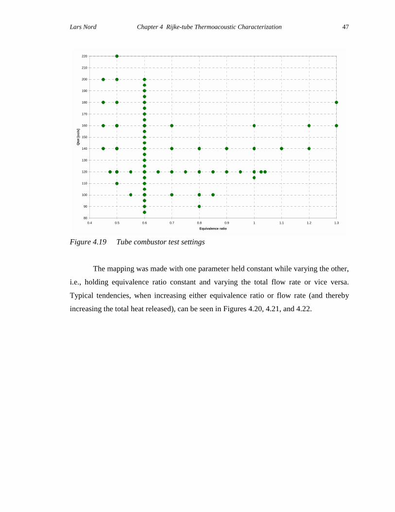
4.6 Extensive Mapping of the Operating Region
The fluctuating pressure, chemiluminescence, and temperatures were measured
for a number of settings, in terms of equivalence ratio and total flow rate. The mapping
was made to provide information about how changes in settings affect the pressure and
OH* power spectra. In addition, an extensive mapping like this can provide helpful
information for anyone who would like to model a closed-open duct with, for example,
CFD. In Figure 4.19, a graph of all the settings used is shown.
Lars Nord Chapter 4 Rijke-tube Thermoacoustic Characterization
47
80
90
100
110
120
130
140
150
160
170
180
190
200
210
220
0.4 0.5 0.6 0.7 0.8 0.9 1 1.1 1.2 1.3
Equivalence ratio
Qto
t [cc
/s]
Figure 4.19 Tube combustor test settings
The mapping was made with one parameter held constant while varying the other,
i.e., holding equivalence ratio constant and varying the total flow rate or vice versa.
Typical tendencies, when increasing either equivalence ratio or flow rate (and thereby
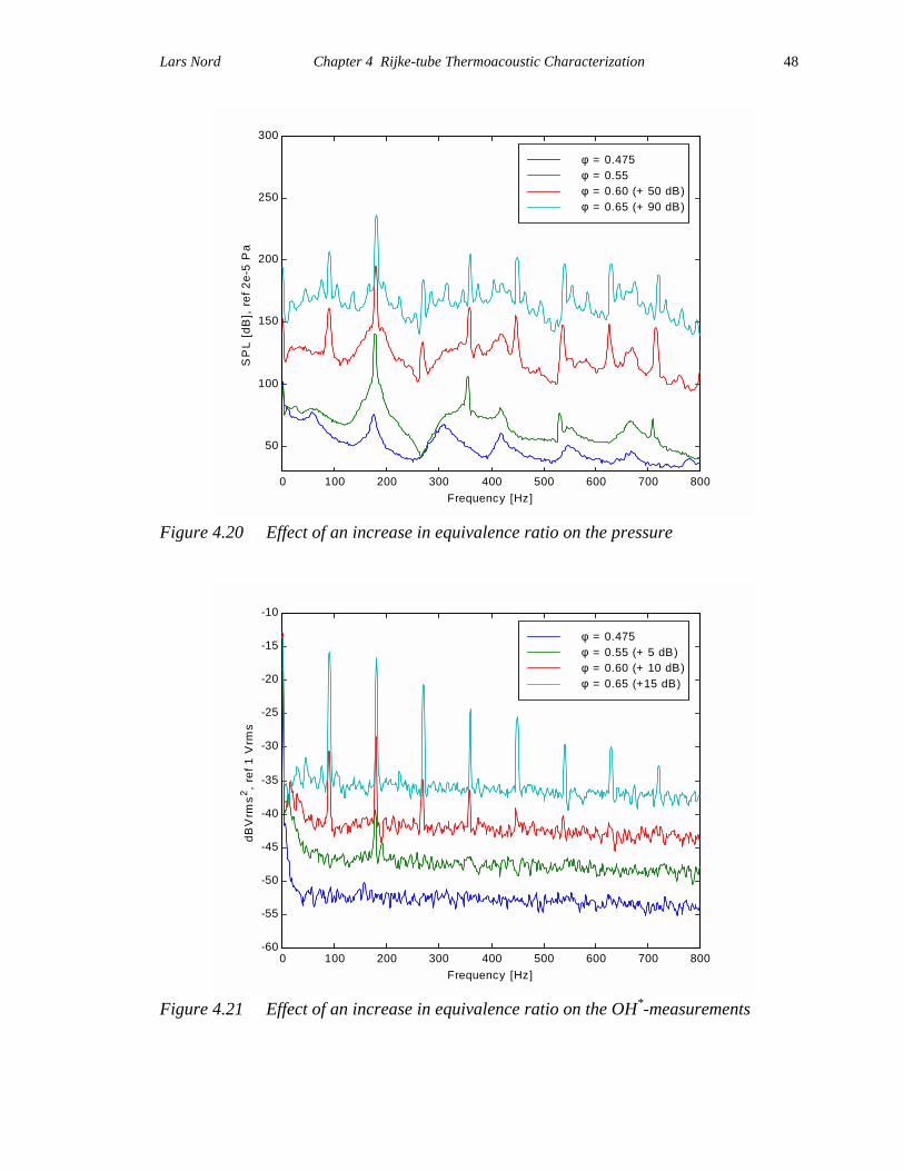
increasing the total heat released), can be seen in Figures 4.20, 4.21, and 4.22.
Lars Nord Chapter 4 Rijke-tube Thermoacoustic Characterization
48
0 100 200 300 400 500 600 700 800
50
100
150
200
250
300
Frequency [Hz]
SP
L [d
B],
ref
2e-
5 P
a
φ = 0.475 φ = 0.55 φ = 0.60 (+ 50 dB)φ = 0.65 (+ 90 dB)
Figure 4.20 Effect of an increase in equivalence ratio on the pressure
0 100 200 300 400 500 600 700 800-60
-55
-50
-45
-40
-35
-30
-25
-20
-15
-10
Frequency [Hz]
dBV
rms2 ,
ref 1
Vrm
s
φ = 0.475 φ = 0.55 (+ 5 dB) φ = 0.60 (+ 10 dB)φ = 0.65 (+15 dB)
Figure 4.21 Effect of an increase in equivalence ratio on the OH*-measurements

Lars Nord Chapter 4 Rijke-tube Thermoacoustic Characterization
49
0
50
100
150
200
250
300
350
400
450
0 10 20 30 40 50 60Axial distance [Inches]
Tem
pera
ture
[C]
Phi = 0.475 Phi = 0.55 Phi = 0.60 Phi = 0.65 Figure 4.22 Effect of an increase in equivalence ratio on the axial temperature profile
Note that the some of the spectra in Figures 4.20 and 4.21 have been shifted
vertically for display purposes. As can be seen in Figure 4.20, for the lowest setting the
heat release is not quite enough to overcome the damping in the tube and to cause a
thermoacoustic instability. Instead we are seeing the tube resonances with the 1st mode
around 55 Hz, the 2nd around 175 Hz, and higher modes at higher frequencies. With a
slight increase in equivalence ratio, and therefore an increase in the heat released, the
instability appears, reaches a limit cycle, and as mentioned before it is the 2nd acoustic
mode that goes unstable. Also visible are the harmonics of the limit cycle. At yet a
higher equivalence ratio, the subharmonic response appears in the spectrum, as well as
harmonics of it. At an even higher equivalence ratio, the pulsating instability is
somewhat visible, and one can see that it modulates the other peaks. The tendency is the
same in Figure 4.21. At the lowest setting there are no peaks visible because the
thermoacoustic instability is not present. With an increase in the equivalence ratio, the
TA instability appears, and is followed by the subharmonic response, the pulsating
instability, and their harmonics for yet higher settings. It is hard to draw any conclusions
from the temperature profiles shown in Figure 4.22. The variations are very small and do
Lars Nord Chapter 4 Rijke-tube Thermoacoustic Characterization
50
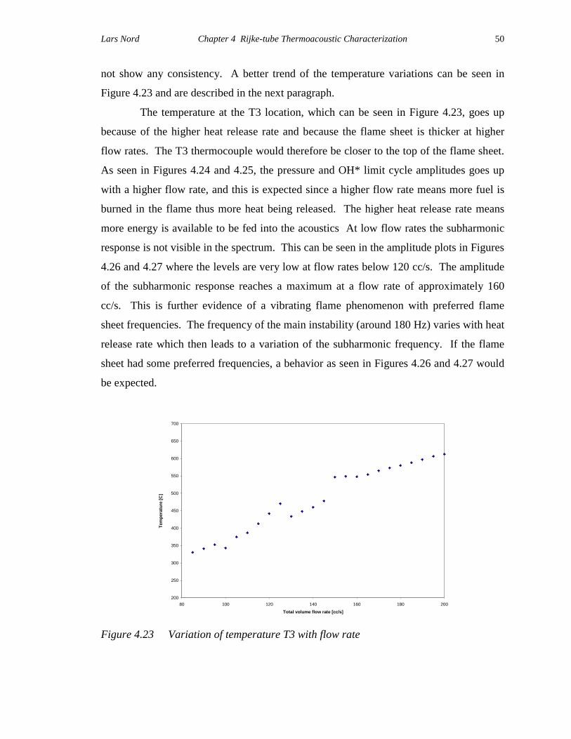
not show any consistency. A better trend of the temperature variations can be seen in
Figure 4.23 and are described in the next paragraph.
The temperature at the T3 location, which can be seen in Figure 4.23, goes up
because of the higher heat release rate and because the flame sheet is thicker at higher
flow rates. The T3 thermocouple would therefore be closer to the top of the flame sheet.
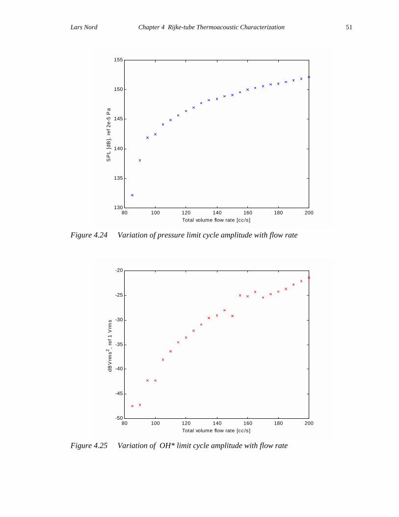
As seen in Figures 4.24 and 4.25, the pressure and OH* limit cycle amplitudes goes up
with a higher flow rate, and this is expected since a higher flow rate means more fuel is
burned in the flame thus more heat being released. The higher heat release rate means
more energy is available to be fed into the acoustics At low flow rates the subharmonic
response is not visible in the spectrum. This can be seen in the amplitude plots in Figures
4.26 and 4.27 where the levels are very low at flow rates below 120 cc/s. The amplitude
of the subharmonic response reaches a maximum at a flow rate of approximately 160
cc/s. This is further evidence of a vibrating flame phenomenon with preferred flame
sheet frequencies. The frequency of the main instability (around 180 Hz) varies with heat
release rate which then leads to a variation of the subharmonic frequency. If the flame
sheet had some preferred frequencies, a behavior as seen in Figures 4.26 and 4.27 would
be expected.
200
250
300
350
400
450
500
550
600
650
700
80 100 120 140 160 180 200
Total volume flow rate [cc/s]
Tem
pera
ture
[C]
Figure 4.23 Variation of temperature T3 with flow rate
Lars Nord Chapter 4 Rijke-tube Thermoacoustic Characterization
51
80 100 120 140 160 180 200130
135
140
145
150
155
Total volume flow rate [cc/s]
SP
L [d
B],
ref
2e-
5 P
a
Figure 4.24 Variation of pressure limit cycle amplitude with flow rate
80 100 120 140 160 180 200-50
-45
-40
-35
-30
-25
-20
Total volume flow rate [cc/s]
dBV
rms2 ,
ref 1
Vrm
s
Figure 4.25 Variation of OH* limit cycle amplitude with flow rate

Lars Nord Chapter 4 Rijke-tube Thermoacoustic Characterization
52
80 100 120 140 160 180 20070
75
80
85
90
95
100
105
110
115
120
Total volume flow rate [cc/s]
SP
L [d
B],
ref
2e-
5 P
a
Figure 4.26 Variation of pressure subharmonic amplitude with flow rate
80 100 120 140 160 180 200-50
-45
-40
-35
-30
-25
-20
Total volume flow rate [cc/s]
dBV
rms2 ,
ref 1
Vrm
s
Figure 4.27 Variation of OH* subharmonic amplitude with flow rate

Lars Nord Chapter 4 Rijke-tube Thermoacoustic Characterization
53
4.7 Database on the World Wide Web
To provide an accesible database for researchers interested in either comparing
data, in terms of pressure power spectra, OH* power spectra, and axial temperature
distribution, or to compare analysis results such as CFD analysis, to data from a Rijke-
type tube combustor, the data has been made available on the WWW. It is possible to
download the data at:
http://www.combustion.me.vt.edu
4.8 Resonance Frequencies The acoustic resonances of the tube combustor have been measured and
calculated. The calculations were made with the wave equation (cold case, i.e., at room
temperature, as described in Chapter 2) and with a first generation finite element method
(FEM) code which sees the tube as a beam (cold case and hot, i.e., at elevated
temperature when combustion is taken place, case). The cold case measurements were
performed by exciting the tube with random noise through a speaker and measuring the
pressure. The hot case measurements were at a low enough setting, in terms of
equivalence ratio and total flow rate, before the thermoacoustic instability had appeared
as seen in Figure 4.28.
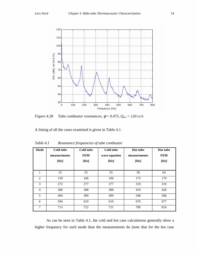
Lars Nord Chapter 4 Rijke-tube Thermoacoustic Characterization
54
0 100 200 300 400 500 600 700 80030
40
50
60
70
80
90
100
110
120
Frequency [Hz]
SP
L [d
B],
ref
2e-
5 P
a
Figure 4.28 Tube combustor resonances, φ = 0.475, Qtot = 120 cc/s
A listing of all the cases examined is given in Table 4.1.
Table 4.1 Resonance frequencies of tube combustor
Mode Cold tube
measurements
[Hz]
Cold tube
FEM
[Hz]
Cold tube
wave equation
[Hz]
Hot tube
measurements
[Hz]
Hot tube
FEM
[Hz]
1 55 55 55 58 64
2 159 166 166 175 179
3 272 277 277 310 319
4 380 388 388 419 428
5 494 499 499 548 568
6 594 610 610 670 677
7 713 722 721 780 816
As can be seen in Table 4.1, the cold and hot case calculations generally show a
higher frequency for each mode than the measurements do (note that for the hot case

Lars Nord Chapter 4 Rijke-tube Thermoacoustic Characterization
55
calculations uncorrected temperatures were used, as discussed in Chapter 3). An
investigation of the cause of the differences was initiated. All the pressure gages were
removed, except for one located in the very bottom of the combustor at location P1, as
seen in Figure 3.1 in Chapter 3. Also, all the thermocouples were removed as well as the
optics system on top of the tube. The speaker, which excited the tube with fixed sine
waves at chosen frequencies, was mounted at locations P4, T6, and P2 respectively in the
tube combustor (refer to Figure 3.1 in Chapter 3). The results are shown in Table 4.2.
Table 4.2 Resonance frequencies of tube combustor without pressure transducers,
thermocouples and optics system
Mode Speaker at P4 location
Frequency [Hz]
Speaker at T6 location
Frequency [Hz]
Speaker at P2 location
Frequency [Hz]
1 * 54 *
2 161 165 163
3 277 276 273
4 380 378 378
5 495 494 496
6 595 595 595
7 714 713 715
* A single frequency was hard to determine. The resonance was spanned over a range of frequencies.
From a comparison of the data in Table 4.1, it can be seen that the results are
slightly closer to the calculated values, but still there is a relatively big difference
between measurements and calculations in forms of the wave equation and the FEM
code. Also worth noting is that the speaker clearly interacts with the tube combustor
which can be because the frequencies shift depending on where the speaker is mounted.
The flame holder in the tube combustor was present in all the above
measurements. To investigate the role of the flame holder it was taken out of the
combustor. The speaker was, as in the previous measurements, mounted at different
locations and the tube was excited with frequency fixed sine waves. The results of these
measurements are presented in Table 4.3.

Lars Nord Chapter 4 Rijke-tube Thermoacoustic Characterization
56
Table 4.3 Resonance frequencies of tube combustor without pressure transducers,
thermocouples, optics system and flame holder
Mode Speaker at P4 location
Frequency [Hz]
Speaker at T6 location
Frequency [Hz]
Speaker at P2 location
Frequency [Hz]
1 * 55 *
2 165 168 166
3 278 277 275
4 386 385 386
5 497 496 497
6 607 606 606
7 714 * 720
* A single frequency was hard to determine. The resonance was spanned over a range of frequencies.
The frequencies are closer to the calculated frequencies than before. The calculations are
now within ± 1% of the measurements.
A frequency response of the speaker with plenum was also taken to get further
knowledge about the tube combustor – speaker interaction. The amplitude and the phase
of the frequency response is shown in Figure 4.29.
Figure 4.29 Frequency response of speaker including plenum
The speaker plenum exhibited resonances at around 60 Hz and 300 Hz as
demonstrated by the magnitude plot as a peak and in the phase plot as a 180 degrees
phase shift. There is also a resonance at a higher frequency, although not well-defined.
0 100 200 300 400 500 600 700 800-90
-80
-70
-60
-50
-40
-30
-20
-10
0
10
Frequency [Hz]
Mag
nitu
de [
dB]
0 100 200 300 400 500 600 700 800-200
-150
-100
-50
0
50
100
150
200
Frequency [Hz]
Pha
se [
deg]

Lars Nord Chapter 4 Rijke-tube Thermoacoustic Characterization
57
The plenum resonances do have an effect on the tube resonances, and are especially
obvious around the 60 Hz area. When the speaker is mounted in locations P2 and P4, the
1st tube resonance gets blurred out. This is possibly due to the speaker plenum’s
resonance in the vicinity of 60 Hz.
58
Chapter 5 Conclusions and Future Work
5.1 Conclusions
All the phenomena that affect the acoustic pressure in a Rijke-type tube
combustor have been experimentally examined in this thesis. In correspondence with
previous research in this area, the Rayleigh Criterion could be verified and proved valid
for the tube combustor in the study. As predicted by theory, the 2nd acoustic mode
became excited with a flame mid-span in a closed-open tube. In addition to
thermoacoustic instabilities caused in accordance with the Rayleigh Criterion, several
other phenomena were observed. With the aid of extensive experimental results, a
vibrating flame and a pulsating flame occurrence have been identified.
All the experimental data collected during this work support the suggested
theories for a vibrating flame as well as a pulsating flame instability. The vibrating flame
occurrence is an oscillating behavior of the flame sheet anchored on the flame-stabilizing
honeycomb in the tube combustor. The flame exhibits mode shapes, as proven by a
bench-top experiment and supported by a variety of experiments with the tube combustor
itself. The flame sheet has preferred frequencies for the mentioned oscillation. In the
Rijke-type tube, the flame sheet is unstable at a frequency of half the forcing function.
The forcing function was, in the case of the tube combustor, the main thermoacoustic
instability in accordance with the Rayleigh Criterion.
The pulsating instability is based on heat losses to the flame stabilizer in
conjunction with changes in flame speed caused by the heat losses. When the flame sheet
is close to the ceramic honeycomb, the heat losses to the honeycomb decrease the flame
temperature which in turn causes a decrease in the flame speed. The forced convection,
which is the unburned mixture flowing downstream, forces the flame sheet upwards in
the tube which then leads to a change in the heat released to the gas from the flame.
When the heat losses to the honeycomb decrease, due to the increased distance, the flame
temperature and therefore the flame speed increases and overcomes the forced
convection. The flame sheet will then move back towards the honeycomb and the
scenario will repeat. The changes in the heat release to the fluid will couple with the
Lars Nord Chapter 5 Conclusions and Future Work
59
acoustics and a peak will show up in the acoustic pressure spectrum. The pulsating
instability of the tube combustor is at a low frequency in the subsonic region. The above
mentioned phenomena were also visible in the chemiluminescence spectrum of the tube
combustor.
To summarize, there are three phenomena evident from the acoustic pressure and
the chemiluminescence measurements of the tube combustor:
- The main thermoacoustic instability, in accordance with the Rayleigh
Criterion, causing the 2nd acoustic mode of the tube to become unstable.
- The vibrating flame instability with flame mode shapes oscillating with a
frequency of half the thermoacoustic instability.
- The pulsating flame instability with an, in the axial direction of the tube
combustor, oscillation caused by the heat losses to the flame stabilizing
honeycomb, typically in the subsonic frequency region.
Extensive data was taken of the whole operating region of the tube combustor in order to
analyze the above described phenomena and to provide a database accessible over the
Internet for researchers interested in comparing experimental data to theoretical
calculations.
5.2 Future Work
While this work was in progress, several researchers in the VACCG conducted
experiments and analyses related to the tube combustor. Much work was focused upon
control issues and analytical models of the combustor and its phenomena. The
compilation of data and analyses presented in this thesis should be attempted for a 3-D
combustor where the acoustics is more complicated and fluid dynamics plays a more vital
part. The instabilities described may also occur in 3-D systems and the understanding of
them would be important in attempting to control the instabilities and in predicting
instability frequencies and amplitude levels. The last step would be to investigate a full-
scale gas turbine combustor used in power plants all over the world. By understanding
the phenomena occurring in a simple tube combustor the likelihood of understanding
them in a full-scale gas turbine combustor is much greater. In order to be able to
Lars Nord Chapter 5 Conclusions and Future Work
60
successfully control the instabilities occurring in a combustor, an understanding of the
physical occurrences is very important.
Typically, gas turbines are dual fuel machines which means they run both on
gaseous fuel (usually natural gas) and liquid fuel (usually fuel oil). It is therefore
important to investigate the thermoacoustic problem also for liquid fuel. This document
only investigated the gas fuel problem which is different from the liquid fuel problem
where such things as fuel atomization, fuel vaporization, and related phenomena occur.
According to Vivek Khanna, member of the VACCG, the correction procedure of
temperatures collected by thermocouples in Rijke-type combustors should be
investigated. The initial correction procedure for the temperature data collected for this
thesis work is not sufficient for these types of combustors. This investigation would be
important for future temperature corrections in Rijke-type combustors and related
devices.
It would also be beneficial to create a CFD model of the tube combustor system to
compare the experimental results with the calculated results.
61
References
Bailey, J. J., “A Type of Flame-Excited Oscillation in a Tube,” Journal of Applied
Mechanics, vol. 24 (1957), pp. 333-339.
Baillot, F., D. Durox, and R. Prud’homme, “Experimental and Theoretical Study of a
Premixed Vibrating Flame,” Combustion and Flame, vol. 88 (1992), pp. 149-168.
Blackshear, P. L., Jr., “Driving Standing Waves by Heat Addition,” Fourth Symposium
(International) on Combustion, pp. 553-566 (1953).
Bloxsidge, G. J., A. P. Dowling, and P. J. Langhorne, “Reheat Buzz: An Acoustically
Coupled Combustion Instability. Part 2. Theory,” The Journal of Fluid Mechanics, vol.
193 (1988), pp. 445-473.
Buckmaster, J., “Stability of the Porous Plug Burner Flame,” SIAM Journal of Applied
Mathematics, vol. 43 (1983), pp. 1335-1349.
Cho, S., J. Kim, and S. Lee, “Characteristics of Thermoacoustic Oscillation in a Ducted
Flame Burner,” AIAA paper 98-0473 (1998).
Clavin, P., and P. Garcia, “The Influence of the Temperature Dependence of Diffusivities
on the Dynamics of Flame Fronts,” Journal de Mécanique Théorique et Appliquée, vol. 2
(1983), pp. 245-263.
Culick, F. E. C., “Combustion Instabilities in Propulsion Systems,” Combustion
Instabilities Driven by Thermoacoustic Sources, NCA vol. 4 (1989) pp. 33-52.
Diederichsen, J., and R. D. Gould, “Combustion Instability: Radiation from Premixed
Flames of Variable Burning Velocity,” Combustion and Flame, vol. 9 (1965), pp. 25-31.
Lars Nord References
62
Durox, D., F. Baillot, G. Searby, and L. Boyer, “On the Shape of Flames Under Strong
Acoustic Forcing: A Mean Flow Controlled by an Oscillating Flow,” Journal of Fluid
Mechanics, vol. 350 (1997), pp. 295-310.
Durox, D., S. Ducruix, and F. Baillot, “Strong Acoustic Forcing on Conical Premixed
Flames,” Twenty-Seventh Symposium (International) on Combustion (1998), pp. 883-889.
Feldman, K. T., Jr., “Review of the Literature on Rijke Thermoacoustic Phenomena,”
Journal of Sound and Vibration, vol. 7 (1968), pp. 83-89.
Gaydon, A. G., The Spectroscopy of Flames, 2nd edition (London: Chapman and Hall,
1974).
Grove, D. E., L. Nord, W. R. Saunders, L. Haber, U. Vandsburger, and C. A. Fannin,
“Tube Combustor Temperature Acquisition System,” VACCG Technical Brief (1998).
Haber, L. C., “An Investigation Into the Origin, Measurement and Application of Chemiluminescent Light Emissions from Premixed Flames,” Master’s Thesis, Virginia Polytechnic Institute and State University (2000).
Hibshman, J. R., “An Experimental Study of Soot Formation in Dual Mode Laminar
Wolfhard-Parker Flames,” Master’s Thesis, Virginia Polytechnic Institute and State
University (1999).
Joos, F., and D. Vortmeyer, “Self-Excited Oscillations in Combustion Chambers with
Premixed Flames and Several Frequencies,” Combustion and Flame, vol. 65 (1986), pp.
253-262.
Kinsler, L. E., A. R. Frey, A. B. Coppens, and J. V. Sanders, Fundamentals of Acoustics,
3rd edition (New York: John Wiley & Sons, 1982).
Lars Nord References
63
Langhorne, P. J., “Reheat Buzz: An Acoustically Coupled Combustion Instability. Part 1.
Experiment,” The Journal of Fluid Mechanics, vol. 193 (1988), pp. 417-443.
Margolis, S. B., “Bifurcation Phenomena in Burner-Stabilized Premixed Flames,”
Combustion Science and Technology, vol. 22 (1980), pp. 143-169.
Markstein, G. H., Nonsteady Flame Propagation (New York: Macmillan, 1964).
Mawardi, O. K., “Aero-Thermoacoustics, the Generation of Sound by Turbulence and by
Heat Processes,” Reports of Progress in Physics, vol. 19 (1956), pp. 156-187.
McIntosh, A. C., and J. F. Clarke, “Second Order Theory of Unsteady Burner-Anchored
Flames With Arbitrary Lewis Number,” Combustion Science and Technology, vol. 38
(1984), pp. 161-196.
McIntosh, A. C., “The Effect of Upstream Acoustic Forcing and Feedback on the
Stability and Resonance Behaviour of Anchored Flames,” Combustion Science and
Technology, vol. 49 (1986), pp. 143-167.
McIntosh, A. C., “Combustion-Acoustic Interaction of a Flat Flame Burner System
Enclosed Within an Open Tube,” Combustion Science and Technology, vol. 54 (1987),
pp. 217-236.
McIntosh, A. C., “Short Communication On Flame Resonances in Tubes,” Combustion
Science and Technology, vol. 69 (1990), pp. 147-152.
McManus, K. R., T Poinsot, and S. M. Candel, “A Review of Active Control of
Combustion Instabilities,” Progress in Energy and Combustion Science, vol. 19 (1993),
pp. 1-29.
Lars Nord References
64
Pelce, P., and P. Clavin, “Influence of Hydrodynamics and Diffusion upon the Stability
Limits of Laminar Premixed Flames,” Journal of Fluid Mechanics, vol. 124 (1982), pp.
219-237.
Putnam, A. A., and W. R. Dennis, “Study of Burner Oscillations of the Organ-Pipe
Type,” Transactions of the ASME, vol. 75 (1953), pp. 15-28.
Putnam, A. A., and W. R. Dennis, “Burner Oscillations of the Gauze-Tone Type,” The
Journal of the Acoustical Society of America, vol. 26 (1954), pp. 716-725.
Putnam, A. A., and W. R. Dennis, “Survey of Organ-Pipe Oscillations in Combustion
Systems,” The Journal of the Acoustical Society of America, vol. 28 (1956), pp. 246-259.
Putnam, A. A., Combustion-Driven Oscillations in Industry (New York: American
Elsevier Publishing Company, 1971).
Raun, R. L., M. W. Beckstead, J. C. Finlinson, and K. P. Brooks, “A Review of Rijke
Tubes, Rijke Burners and Related Devices,” Progress in Energy and Combstion Science,
vol. 19 (1993), pp. 313-364.
Rayleigh, Lord, “The Explanation of Certain Acoustical Phenomena,” Nature, vol. 18
(1878), pp. 319-321.
Rayleigh, Lord, The Theory of Sound, vol. II, 2nd edition (London: Macmillan, 1926).
Richards, J. S., W. R. Saunders, C. A. Fannin, and L. Nord, “Calibration of the SLP004D
Pressure Transducer for Use in the Tube Combustor,” VACCG Technical Brief (1998).
Rijke, P. L., “Notice of a New Method of Causing a Vibration of the Air Contained in a
Tube Open at Both Ends,” Philosophical Magazine, vol. 17 (1859), pp. 419-422.
Lars Nord References
65
Searby, G., and P. Clavin, “Weakly Turbulent, Wrinkled Flames in Premixed Gases,”
Combustion Science and Technology, vol. 46 (1986), pp. 167-193.
Searby, G., and D. Rochwerger, “A Parametric Acoustic Instability in Premixed Flames,”
Journal of Fluid Mechanics, vol. 231 (1991), pp. 529-543.
Van Harten, A., A. K. Kapila, and B. J. Matkowsky, “Acoustic Coupling of Flames,”
SIAM Journal of Applied Mathematics, vol. 43, no. 5 (October 1984), pp. 982-995.
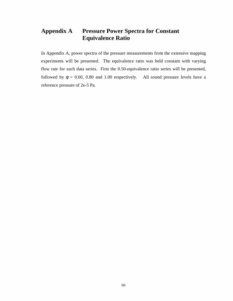
66
Appendix A Pressure Power Spectra for Constant Equivalence Ratio
In Appendix A, power spectra of the pressure measurements from the extensive mapping
experiments will be presented. The equivalence ratio was held constant with varying
flow rate for each data series. First the 0.50-equivalence ratio series will be presented,
followed by φ = 0.60, 0.80 and 1.00 respectively. All sound pressure levels have a
reference pressure of 2e-5 Pa.

Lars Nord Appendix A Pressure Power Spectra for Constant Equivalence Ratio
67
0 100 200 300 400 500 600 700 800
40
60
80
100
120
140
160Power Spectrum p1, phi=0.50, Qtot=110 cc/s
Frequency [Hz]
SP
L [d
B]
Figure A.1 Pressure power spectrum for φ = 0.50, Qtot=110 cc/s
0 100 200 300 400 500 600 700 800
40
60
80
100
120
140
160Power Spectrum p1, phi=0.50, Qtot=120 cc/s
Frequency [Hz]
SP
L [d
B]
Figure A.2 Pressure power spectrum for φ = 0.50, Qtot=120 cc/s
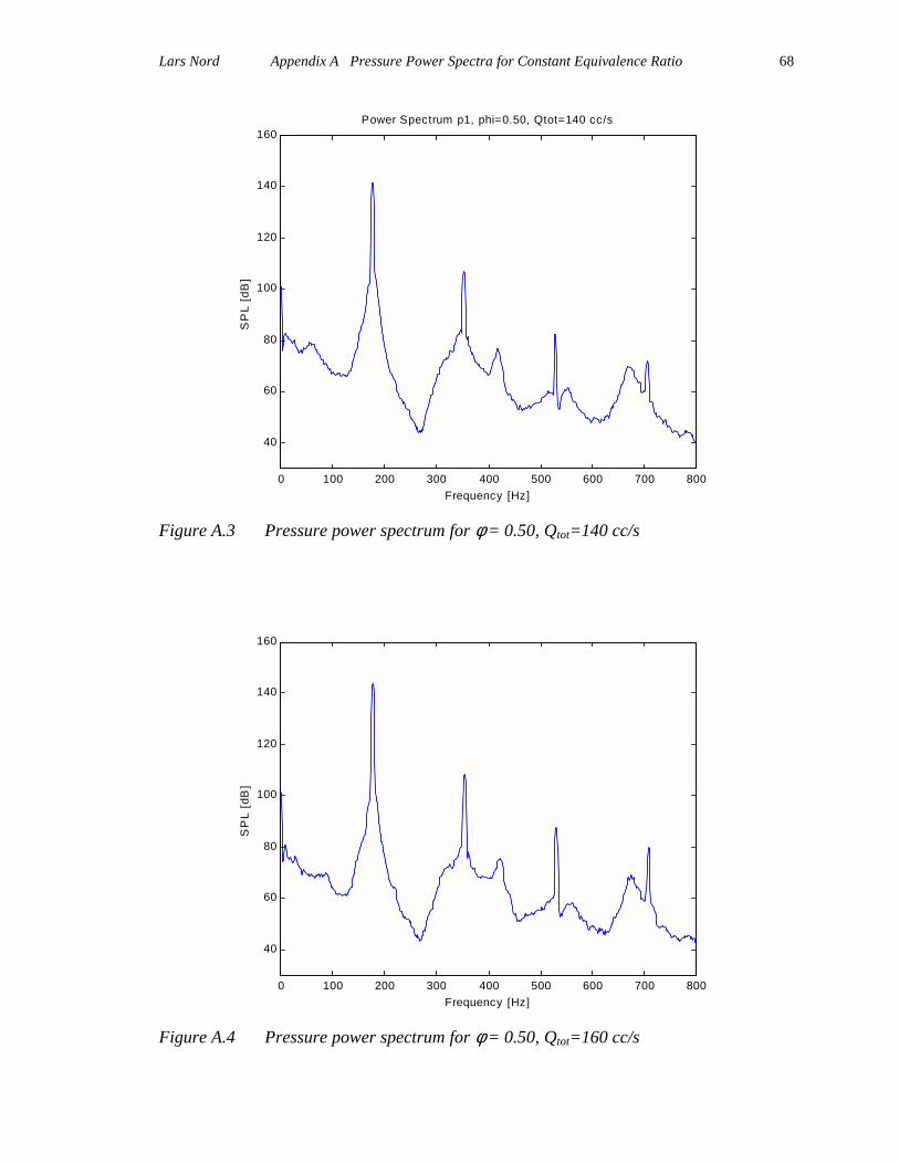
Lars Nord Appendix A Pressure Power Spectra for Constant Equivalence Ratio
68
0 100 200 300 400 500 600 700 800
40
60
80
100
120
140
160Power Spectrum p1, phi=0.50, Qtot=140 cc/s
Frequency [Hz]
SP
L [d
B]
Figure A.3 Pressure power spectrum for φ = 0.50, Qtot=140 cc/s
0 100 200 300 400 500 600 700 800
40
60
80
100
120
140
160
Frequency [Hz]
SP
L [d
B]
Figure A.4 Pressure power spectrum for φ = 0.50, Qtot=160 cc/s
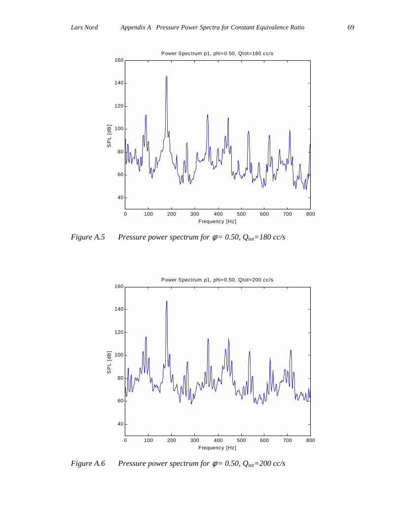
Lars Nord Appendix A Pressure Power Spectra for Constant Equivalence Ratio
69
0 100 200 300 400 500 600 700 800
40
60
80
100
120
140
160Power Spectrum p1, phi=0.50, Qtot=180 cc/s
Frequency [Hz]
SP
L [d
B]
Figure A.5 Pressure power spectrum for φ = 0.50, Qtot=180 cc/s
0 100 200 300 400 500 600 700 800
40
60
80
100
120
140
160Power Spectrum p1, phi=0.50, Qtot=200 cc/s
Frequency [Hz]
SP
L [d
B]
Figure A.6 Pressure power spectrum for φ = 0.50, Qtot=200 cc/s
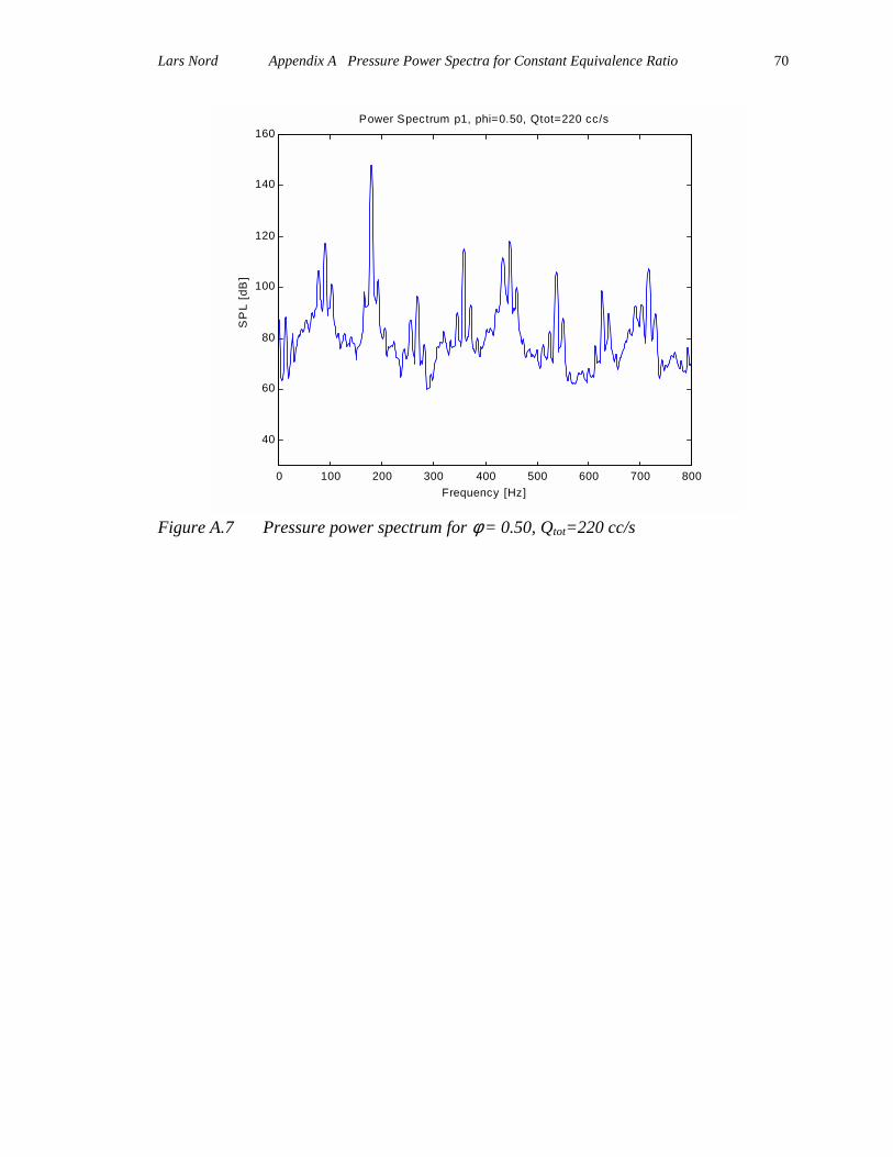
Lars Nord Appendix A Pressure Power Spectra for Constant Equivalence Ratio
70
0 100 200 300 400 500 600 700 800
40
60
80
100
120
140
160Power Spectrum p1, phi=0.50, Qtot=220 cc/s
Frequency [Hz]
SP
L [d
B]
Figure A.7 Pressure power spectrum for φ = 0.50, Qtot=220 cc/s
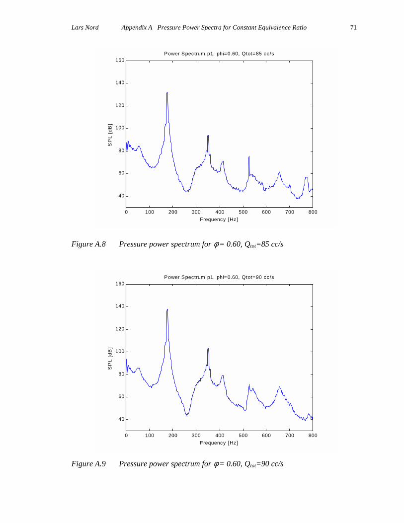
Lars Nord Appendix A Pressure Power Spectra for Constant Equivalence Ratio
71
Figure A.8 Pressure power spectrum for φ = 0.60, Qtot=85 cc/s
Figure A.9 Pressure power spectrum for φ = 0.60, Qtot=90 cc/s
0 100 200 300 400 500 600 700 800
40
60
80
100
120
140
160Power Spectrum p1, phi=0.60, Qtot=85 cc/s
Frequency [Hz]
SP
L [d
B]
0 100 200 300 400 500 600 700 800
40
60
80
100
120
140
160Power Spectrum p1, phi=0.60, Qtot=90 cc/s
Frequency [Hz]
SP
L [d
B]
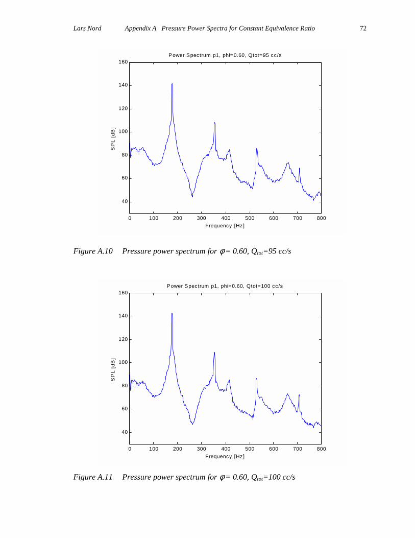
Lars Nord Appendix A Pressure Power Spectra for Constant Equivalence Ratio
72
Figure A.10 Pressure power spectrum for φ = 0.60, Qtot=95 cc/s
Figure A.11 Pressure power spectrum for φ = 0.60, Qtot=100 cc/s
0 100 200 300 400 500 600 700 800
40
60
80
100
120
140
160Power Spectrum p1, phi=0.60, Qtot=95 cc/s
Frequency [Hz]
SP
L [d
B]
0 100 200 300 400 500 600 700 800
40
60
80
100
120
140
160Power Spectrum p1, phi=0.60, Qtot=100 cc/s
Frequency [Hz]
SP
L [d
B]
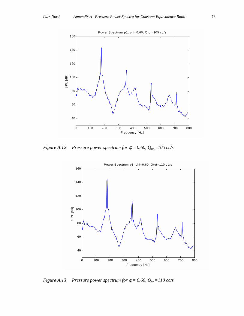
Lars Nord Appendix A Pressure Power Spectra for Constant Equivalence Ratio
73
Figure A.12 Pressure power spectrum for φ = 0.60, Qtot=105 cc/s
Figure A.13 Pressure power spectrum for φ = 0.60, Qtot=110 cc/s
0 100 200 300 400 500 600 700 800
40
60
80
100
120
140
160Power Spectrum p1, phi=0.60, Qtot=105 cc/s
Frequency [Hz]
SP
L [d
B]
0 100 200 300 400 500 600 700 800
40
60
80
100
120
140
160Power Spectrum p1, phi=0.60, Qtot=110 cc/s
Frequency [Hz]
SP
L [d
B]

Lars Nord Appendix A Pressure Power Spectra for Constant Equivalence Ratio
74
Figure A.14 Pressure power spectrum for φ = 0.60, Qtot=115 cc/s
Figure A.15 Pressure power spectrum for φ = 0.60, Qtot=120 cc/s
0 100 200 300 400 500 600 700 800
40
60
80
100
120
140
160Power Spectrum p1, phi=0.60, Qtot=115 cc/s
Frequency [Hz]
SP
L [d
B]
0 100 200 300 400 500 600 700 800
40
60
80
100
120
140
160Power Spectrum p1, phi=0.60, Qtot=120 cc/s
Frequency [Hz]
SP
L [d
B]
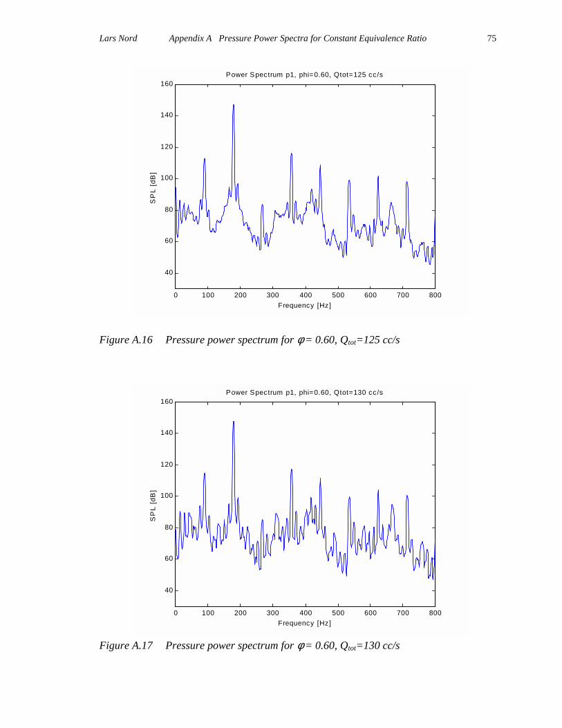
Lars Nord Appendix A Pressure Power Spectra for Constant Equivalence Ratio
75
Figure A.16 Pressure power spectrum for φ = 0.60, Qtot=125 cc/s
Figure A.17 Pressure power spectrum for φ = 0.60, Qtot=130 cc/s
0 100 200 300 400 500 600 700 800
40
60
80
100
120
140
160Power Spectrum p1, phi=0.60, Qtot=125 cc/s
Frequency [Hz]
SP
L [d
B]
0 100 200 300 400 500 600 700 800
40
60
80
100
120
140
160Power Spectrum p1, phi=0.60, Qtot=130 cc/s
Frequency [Hz]
SP
L [d
B]

Lars Nord Appendix A Pressure Power Spectra for Constant Equivalence Ratio
76
Figure A.18 Pressure power spectrum for φ = 0.60, Qtot=135 cc/s
Figure A.19 Pressure power spectrum for φ = 0.60, Qtot=140 cc/s
0 100 200 300 400 500 600 700 800
40
60
80
100
120
140
160Power Spectrum p1, phi=0.60, Qtot=135 cc/s
Frequency [Hz]
SP
L [d
B]
0 100 200 300 400 500 600 700 800
40
60
80
100
120
140
160Power Spectrum p1, phi=0.60, Qtot=140 cc/s
Frequency [Hz]
SP
L [d
B]

Lars Nord Appendix A Pressure Power Spectra for Constant Equivalence Ratio
77
Figure A.20 Pressure power spectrum for φ = 0.60, Qtot=145 cc/s
Figure A.21 Pressure power spectrum for φ = 0.60, Qtot=150 cc/s
0 100 200 300 400 500 600 700 800
40
60
80
100
120
140
160Power Spectrum p1, phi=0.60, Qtot=145 cc/s
Frequency [Hz]
SP
L [d
B]
0 100 200 300 400 500 600 700 800
40
60
80
100
120
140
160Power Spectrum p1, phi=0.60, Qtot=150 cc/s
Frequency [Hz]
SP
L [d
B]
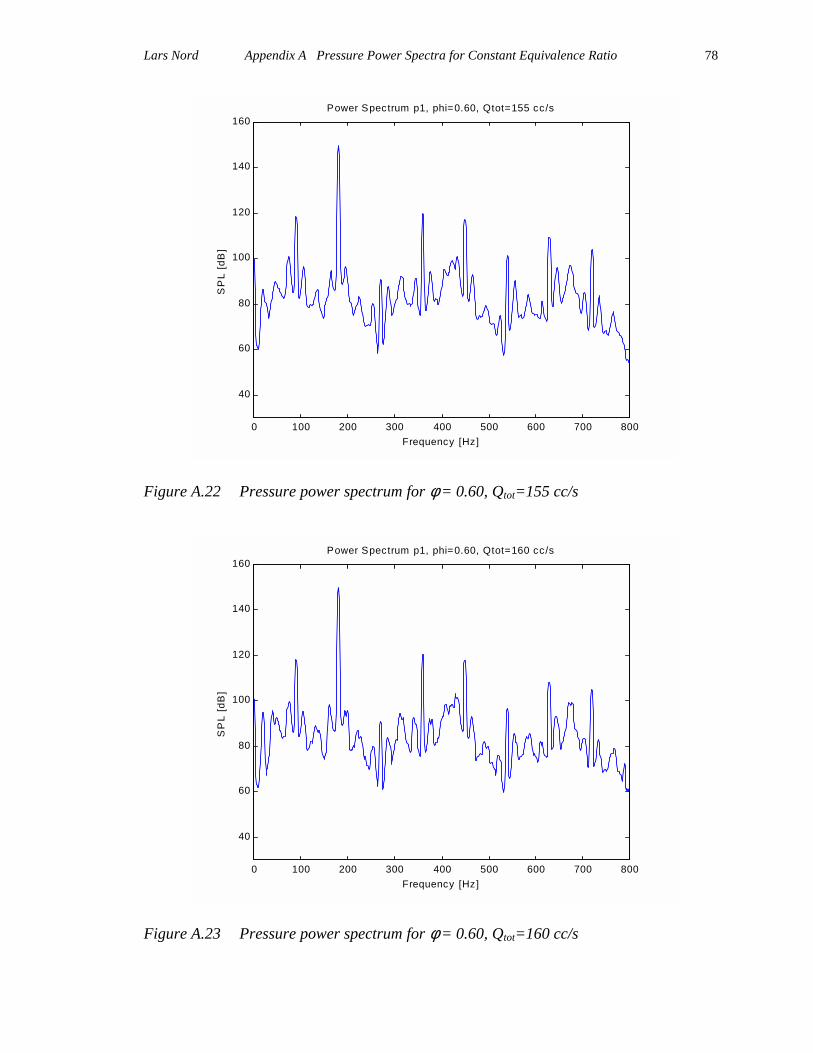
Lars Nord Appendix A Pressure Power Spectra for Constant Equivalence Ratio
78
Figure A.22 Pressure power spectrum for φ = 0.60, Qtot=155 cc/s
Figure A.23 Pressure power spectrum for φ = 0.60, Qtot=160 cc/s
0 100 200 300 400 500 600 700 800
40
60
80
100
120
140
160Power Spectrum p1, phi=0.60, Qtot=155 cc/s
Frequency [Hz]
SP
L [d
B]
0 100 200 300 400 500 600 700 800
40
60
80
100
120
140
160Power Spectrum p1, phi=0.60, Qtot=160 cc/s
Frequency [Hz]
SP
L [d
B]

Lars Nord Appendix A Pressure Power Spectra for Constant Equivalence Ratio
79
0 100 200 300 400 500 600 700 800
40
60
80
100
120
140
160Power Spectrum p1, phi=0.60, Qtot=165 cc/s
Frequency [Hz]
SP
L [d
B]
Figure A.24 Pressure power spectrum for φ = 0.60, Qtot=165 cc/s
0 100 200 300 400 500 600 700 800
40
60
80
100
120
140
160Power Spectrum p1, phi=0.60, Qtot=170 cc/s
Frequency [Hz]
SP
L [d
B]
Figure A.25 Pressure power spectrum for φ = 0.60, Qtot=170 cc/s
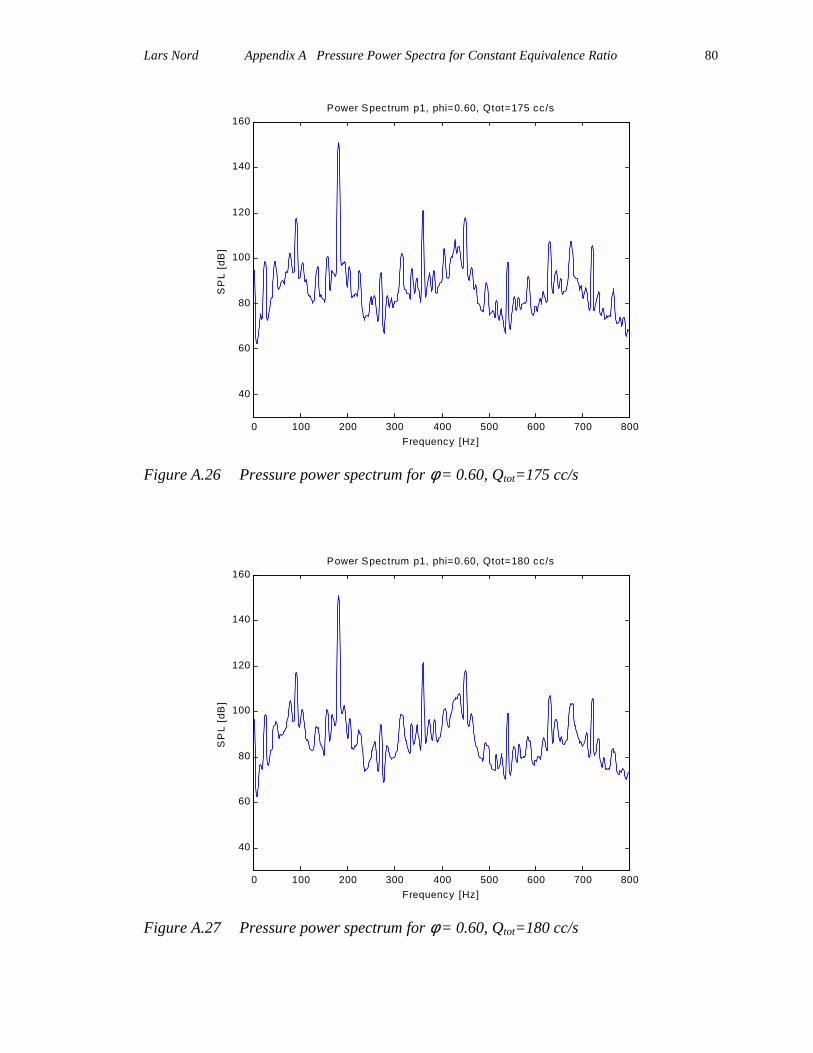
Lars Nord Appendix A Pressure Power Spectra for Constant Equivalence Ratio
80
0 100 200 300 400 500 600 700 800
40
60
80
100
120
140
160Power Spectrum p1, phi=0.60, Qtot=175 cc/s
Frequency [Hz]
SP
L [d
B]
Figure A.26 Pressure power spectrum for φ = 0.60, Qtot=175 cc/s
0 100 200 300 400 500 600 700 800
40
60
80
100
120
140
160Power Spectrum p1, phi=0.60, Qtot=180 cc/s
Frequency [Hz]
SP
L [d
B]
Figure A.27 Pressure power spectrum for φ = 0.60, Qtot=180 cc/s

Lars Nord Appendix A Pressure Power Spectra for Constant Equivalence Ratio
81
0 100 200 300 400 500 600 700 800
40
60
80
100
120
140
160Power Spectrum p1, phi=0.60, Qtot=185 cc/s
Frequency [Hz]
SP
L [d
B]
Figure A.28 Pressure power spectrum for φ = 0.60, Qtot=185 cc/s
0 100 200 300 400 500 600 700 800
40
60
80
100
120
140
160Power Spectrum p1, phi=0.60, Qtot=190 cc/s
Frequency [Hz]
SP
L [d
B]
Figure A.29 Pressure power spectrum for φ = 0.60, Qtot=190 cc/s

Lars Nord Appendix A Pressure Power Spectra for Constant Equivalence Ratio
82
Figure A.30 Pressure power spectrum for φ = 0.60, Qtot=195 cc/s
Figure A.31 Pressure power spectrum for φ = 0.60, Qtot=200 cc/s
0 100 200 300 400 500 600 700 800
40
60
80
100
120
140
160Power Spectrum p1, phi=0.60, Qtot=195 cc/s
Frequency [Hz]
SP
L [d
B]
0 100 200 300 400 500 600 700 800
40
60
80
100
120
140
160Power Spectrum p1, phi=0.60, Qtot=200 cc/s
Frequency [Hz]
SP
L [d
B]
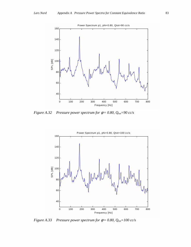
Lars Nord Appendix A Pressure Power Spectra for Constant Equivalence Ratio
83
0 100 200 300 400 500 600 700 800
40
60
80
100
120
140
160Power Spectrum p1, phi=0.80, Qtot=90 cc/s
Frequency [Hz]
SP
L [d
B]
Figure A.32 Pressure power spectrum for φ = 0.80, Qtot=90 cc/s
0 100 200 300 400 500 600 700 800
40
60
80
100
120
140
160Power Spectrum p1, phi=0.80, Qtot=100 cc/s
Frequency [Hz]
SP
L [d
B]
Figure A.33 Pressure power spectrum for φ = 0.80, Qtot=100 cc/s
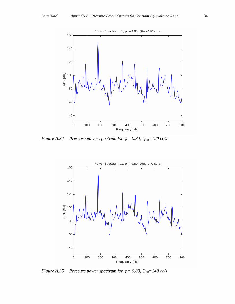
Lars Nord Appendix A Pressure Power Spectra for Constant Equivalence Ratio
84
0 100 200 300 400 500 600 700 800
40
60
80
100
120
140
160Power Spectrum p1, phi=0.80, Qtot=120 cc/s
Frequency [Hz]
SP
L [d
B]
Figure A.34 Pressure power spectrum for φ = 0.80, Qtot=120 cc/s
0 100 200 300 400 500 600 700 800
40
60
80
100
120
140
160Power Spectrum p1, phi=0.80, Qtot=140 cc/s
Frequency [Hz]
SP
L [d
B]
Figure A.35 Pressure power spectrum for φ = 0.80, Qtot=140 cc/s

Lars Nord Appendix A Pressure Power Spectra for Constant Equivalence Ratio
85
Figure A.36 Pressure power spectrum for φ = 1.00, Qtot=115 cc/s
Figure A.37 Pressure power spectrum for φ = 1.00, Qtot=120 cc/s
0 100 200 300 400 500 600 700 800
40
60
80
100
120
140
160Power Spectrum p1, phi=1.00, Qtot=115 cc/s
Frequency [Hz]
SP
L [d
B]
0 100 200 300 400 500 600 700 800
40
60
80
100
120
140
160Power Spectrum p1, phi=1.00, Qtot=120 cc/s
Frequency [Hz]
SP
L [d
B]

Lars Nord Appendix A Pressure Power Spectra for Constant Equivalence Ratio
86
Figure A.38 Pressure power spectrum for φ = 1.00, Qtot=140 cc/s
Figure A.39 Pressure power spectrum for φ = 1.00, Qtot=160 cc/s\
0 100 200 300 400 500 600 700 800
40
60
80
100
120
140
160Power Spectrum p1, phi=1.00, Qtot=140 cc/s
Frequency [Hz]
SP
L [d
B]
0 100 200 300 400 500 600 700 800
40
60
80
100
120
140
160Power Spectrum p1, phi=1.00, Qtot=160 cc/s
Frequency [Hz]
SP
L [d
B]
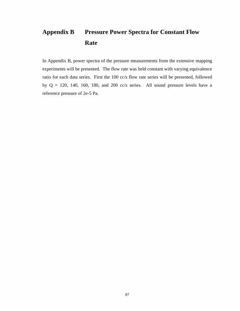
87
Appendix B Pressure Power Spectra for Constant Flow
Rate
In Appendix B, power spectra of the pressure measurements from the extensive mapping
experiments will be presented. The flow rate was held constant with varying equivalence
ratio for each data series. First the 100 cc/s flow rate series will be presented, followed
by Q = 120, 140, 160, 180, and 200 cc/s series. All sound pressure levels have a
reference pressure of 2e-5 Pa.

Lars Nord Appendix B Pressure Power Spectra for Constant Flow Rate
88
Figure B.1 Pressure power spectrum for φ = 0.55, Qtot=100 cc/s
Figure B.2 Pressure power spectrum for φ = 0.60, Qtot=100 cc/s
0 100 200 300 400 500 600 700 800
40
60
80
100
120
140
160Power Spectrum p1, phi=0.55, Qtot=100 cc/s
Frequency [Hz]
SP
L [d
B]
0 100 200 300 400 500 600 700 800
40
60
80
100
120
140
160Power Spectrum p1, phi=0.60, Qtot=100 cc/s
Frequency [Hz]
SP
L [d
B]
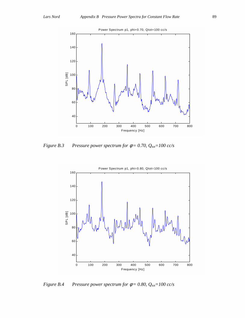
Lars Nord Appendix B Pressure Power Spectra for Constant Flow Rate
89
Figure B.3 Pressure power spectrum for φ = 0.70, Qtot=100 cc/s
Figure B.4 Pressure power spectrum for φ = 0.80, Qtot=100 cc/s
0 100 200 300 400 500 600 700 800
40
60
80
100
120
140
160Power Spectrum p1, phi=0.70, Qtot=100 cc/s
Frequency [Hz]
SP
L [d
B]
0 100 200 300 400 500 600 700 800
40
60
80
100
120
140
160Power Spectrum p1, phi=0.80, Qtot=100 cc/s
Frequency [Hz]
SP
L [d
B]

Lars Nord Appendix B Pressure Power Spectra for Constant Flow Rate
90
Figure B.5 Pressure power spectrum for φ = 0.85, Qtot=100 cc/s
0 100 200 300 400 500 600 700 800
40
60
80
100
120
140
160Power Spectrum p1, phi=0.85, Qtot=100 cc/s
Frequency [Hz]
SP
L [d
B]

Lars Nord Appendix B Pressure Power Spectra for Constant Flow Rate
91
Figure B.6 Pressure power spectrum for φ = 0.475, Qtot=120 cc/s
Figure B.7 Pressure power spectrum for φ = 0.50, Qtot=120 cc/s
0 100 200 300 400 500 600 700 800
40
60
80
100
120
140
160Power Spectrum p1, phi=0.475, Qtot=120 cc/s
Frequency [Hz]
SP
L [d
B]
0 100 200 300 400 500 600 700 800
40
60
80
100
120
140
160Power Spectrum p1, phi=0.50, Qtot=120 cc/s
Frequency [Hz]
SP
L [d
B]
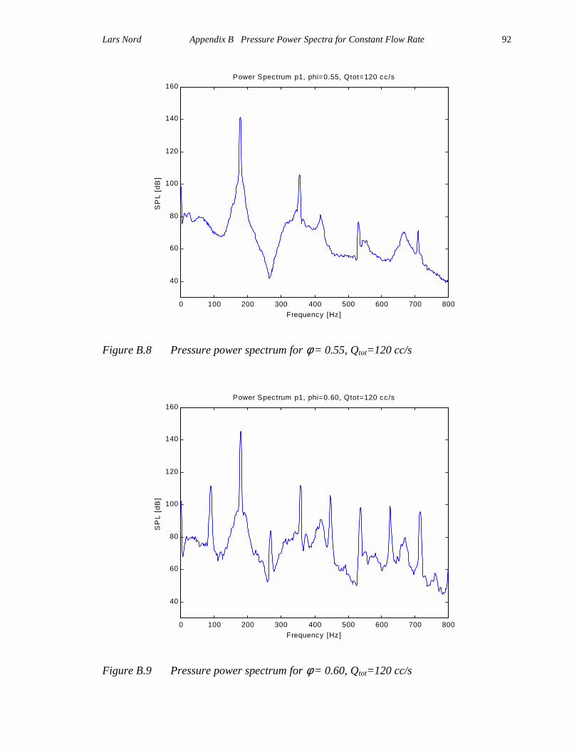
Lars Nord Appendix B Pressure Power Spectra for Constant Flow Rate
92
Figure B.8 Pressure power spectrum for φ = 0.55, Qtot=120 cc/s
Figure B.9 Pressure power spectrum for φ = 0.60, Qtot=120 cc/s
0 100 200 300 400 500 600 700 800
40
60
80
100
120
140
160Power Spectrum p1, phi=0.55, Qtot=120 cc/s
Frequency [Hz]
SP
L [d
B]
0 100 200 300 400 500 600 700 800
40
60
80
100
120
140
160Power Spectrum p1, phi=0.60, Qtot=120 cc/s
Frequency [Hz]
SP
L [d
B]
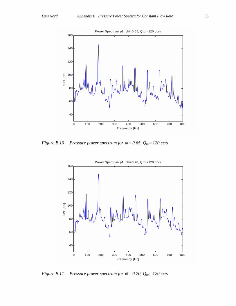
Lars Nord Appendix B Pressure Power Spectra for Constant Flow Rate
93
Figure B.10 Pressure power spectrum for φ = 0.65, Qtot=120 cc/s
Figure B.11 Pressure power spectrum for φ = 0.70, Qtot=120 cc/s
0 100 200 300 400 500 600 700 800
40
60
80
100
120
140
160Power Spectrum p1, phi=0.65, Qtot=120 cc/s
Frequency [Hz]
SP
L [d
B]
0 100 200 300 400 500 600 700 800
40
60
80
100
120
140
160Power Spectrum p1, phi=0.70, Qtot=120 cc/s
Frequency [Hz]
SP
L [d
B]
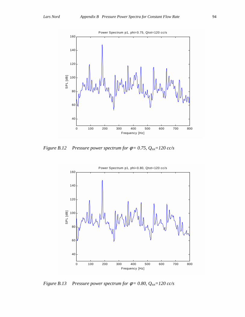
Lars Nord Appendix B Pressure Power Spectra for Constant Flow Rate
94
Figure B.12 Pressure power spectrum for φ = 0.75, Qtot=120 cc/s
Figure B.13 Pressure power spectrum for φ = 0.80, Qtot=120 cc/s
0 100 200 300 400 500 600 700 800
40
60
80
100
120
140
160Power Spectrum p1, phi=0.75, Qtot=120 cc/s
Frequency [Hz]
SP
L [d
B]
0 100 200 300 400 500 600 700 800
40
60
80
100
120
140
160Power Spectrum p1, phi=0.80, Qtot=120 cc/s
Frequency [Hz]
SP
L [d
B]
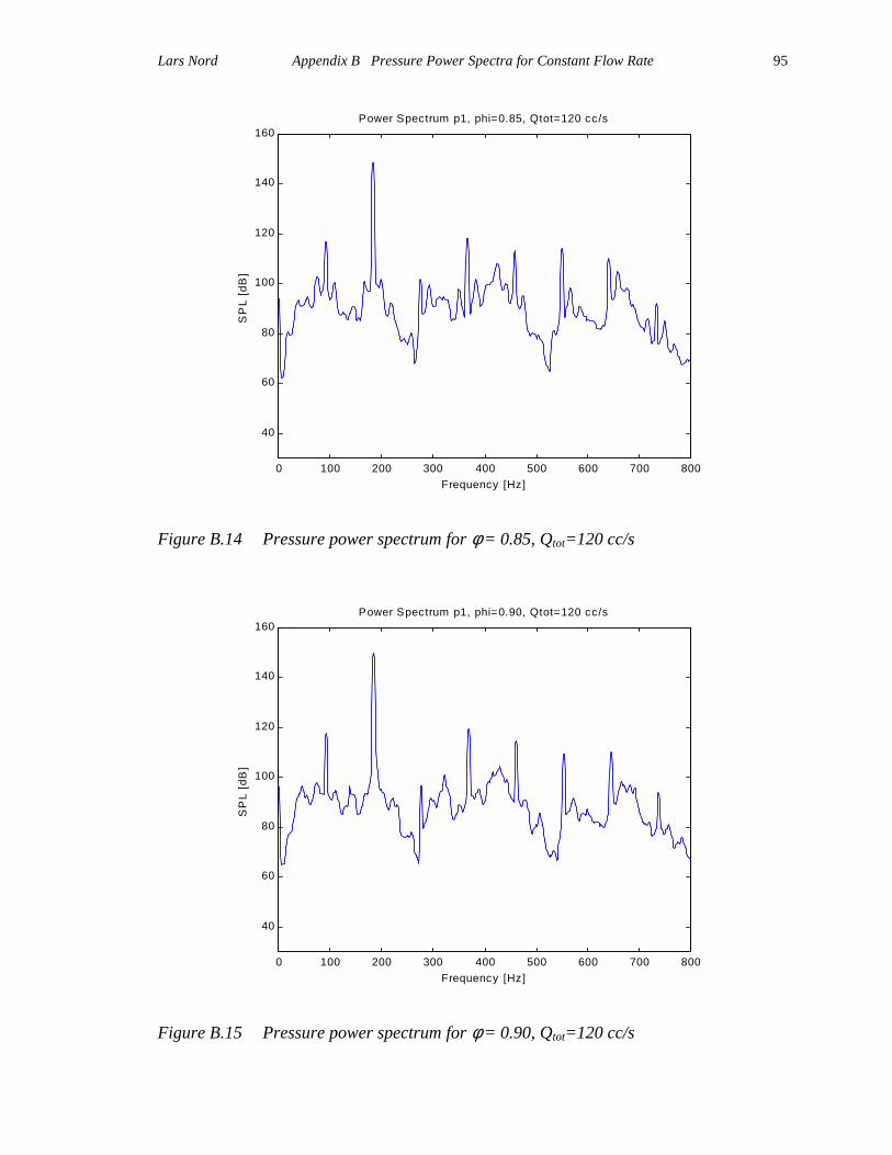
Lars Nord Appendix B Pressure Power Spectra for Constant Flow Rate
95
Figure B.14 Pressure power spectrum for φ = 0.85, Qtot=120 cc/s
Figure B.15 Pressure power spectrum for φ = 0.90, Qtot=120 cc/s
0 100 200 300 400 500 600 700 800
40
60
80
100
120
140
160Power Spectrum p1, phi=0.85, Qtot=120 cc/s
Frequency [Hz]
SP
L [d
B]
0 100 200 300 400 500 600 700 800
40
60
80
100
120
140
160Power Spectrum p1, phi=0.90, Qtot=120 cc/s
Frequency [Hz]
SP
L [d
B]
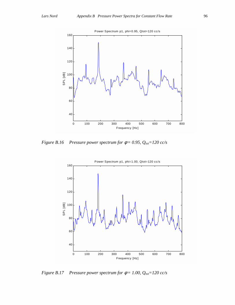
Lars Nord Appendix B Pressure Power Spectra for Constant Flow Rate
96
Figure B.16 Pressure power spectrum for φ = 0.95, Qtot=120 cc/s
Figure B.17 Pressure power spectrum for φ = 1.00, Qtot=120 cc/s
0 100 200 300 400 500 600 700 800
40
60
80
100
120
140
160Power Spectrum p1, phi=0.95, Qtot=120 cc/s
Frequency [Hz]
SP
L [d
B]
0 100 200 300 400 500 600 700 800
40
60
80
100
120
140
160Power Spectrum p1, phi=1.00, Qtot=120 cc/s
Frequency [Hz]
SP
L [d
B]
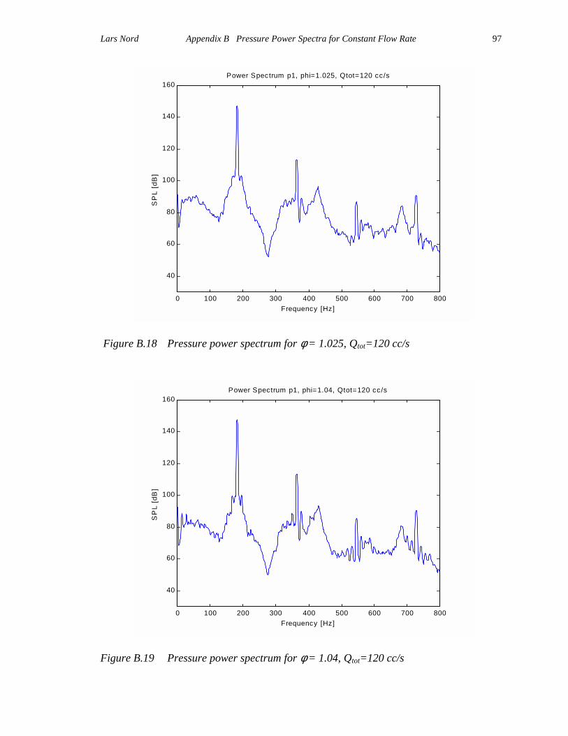
Lars Nord Appendix B Pressure Power Spectra for Constant Flow Rate
97
Figure B.18 Pressure power spectrum for φ = 1.025, Qtot=120 cc/s
Figure B.19 Pressure power spectrum for φ = 1.04, Qtot=120 cc/s
0 100 200 300 400 500 600 700 800
40
60
80
100
120
140
160Power Spectrum p1, phi=1.025, Qtot=120 cc/s
Frequency [Hz]
SP
L [d
B]
0 100 200 300 400 500 600 700 800
40
60
80
100
120
140
160Power Spectrum p1, phi=1.04, Qtot=120 cc/s
Frequency [Hz]
SP
L [d
B]
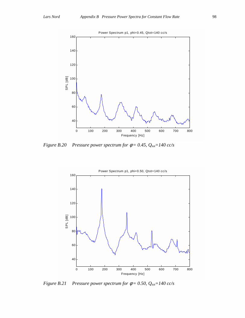
Lars Nord Appendix B Pressure Power Spectra for Constant Flow Rate
98
0 100 200 300 400 500 600 700 800
40
60
80
100
120
140
160Power Spectrum p1, phi=0.45, Qtot=140 cc/s
Frequency [Hz]
SP
L [d
B]
Figure B.20 Pressure power spectrum for φ = 0.45, Qtot=140 cc/s
0 100 200 300 400 500 600 700 800
40
60
80
100
120
140
160Power Spectrum p1, phi=0.50, Qtot=140 cc/s
Frequency [Hz]
SP
L [d
B]
Figure B.21 Pressure power spectrum for φ = 0.50, Qtot=140 cc/s
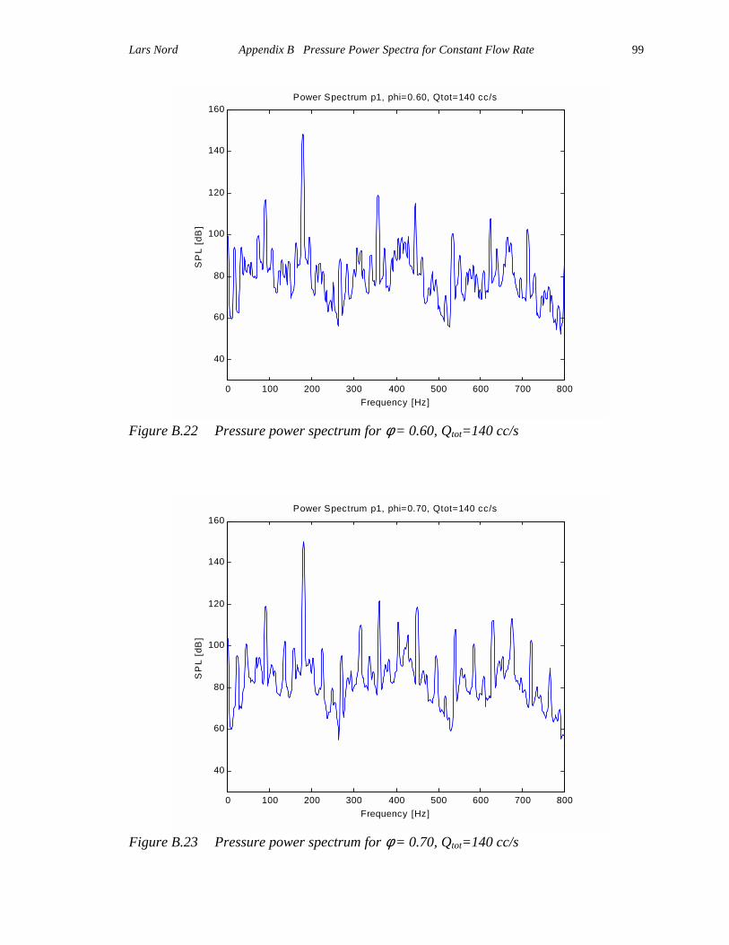
Lars Nord Appendix B Pressure Power Spectra for Constant Flow Rate
99
0 100 200 300 400 500 600 700 800
40
60
80
100
120
140
160Power Spectrum p1, phi=0.60, Qtot=140 cc/s
Frequency [Hz]
SP
L [d
B]
Figure B.22 Pressure power spectrum for φ = 0.60, Qtot=140 cc/s
0 100 200 300 400 500 600 700 800
40
60
80
100
120
140
160Power Spectrum p1, phi=0.70, Qtot=140 cc/s
Frequency [Hz]
SP
L [d
B]
Figure B.23 Pressure power spectrum for φ = 0.70, Qtot=140 cc/s

Lars Nord Appendix B Pressure Power Spectra for Constant Flow Rate
100
0 100 200 300 400 500 600 700 800
40
60
80
100
120
140
160Power Spectrum p1, phi=0.80, Qtot=140 cc/s
Frequency [Hz]
SP
L [d
B]
Figure B.24 Pressure power spectrum for φ = 0.80, Qtot=140 cc/s
0 100 200 300 400 500 600 700 800
40
60
80
100
120
140
160Power Spectrum p1, phi=0.90, Qtot=140 cc/s
Frequency [Hz]
SP
L [d
B]
Figure B.25 Pressure power spectrum for φ = 0.90, Qtot=140 cc/s
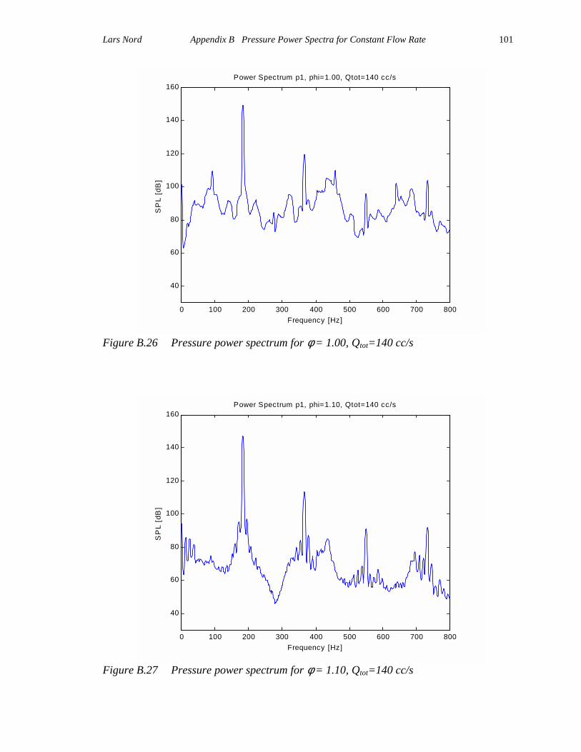
Lars Nord Appendix B Pressure Power Spectra for Constant Flow Rate
101
0 100 200 300 400 500 600 700 800
40
60
80
100
120
140
160Power Spectrum p1, phi=1.00, Qtot=140 cc/s
Frequency [Hz]
SP
L [d
B]
Figure B.26 Pressure power spectrum for φ = 1.00, Qtot=140 cc/s
0 100 200 300 400 500 600 700 800
40
60
80
100
120
140
160Power Spectrum p1, phi=1.10, Qtot=140 cc/s
Frequency [Hz]
SP
L [d
B]
Figure B.27 Pressure power spectrum for φ = 1.10, Qtot=140 cc/s

Lars Nord Appendix B Pressure Power Spectra for Constant Flow Rate
102
0 100 200 300 400 500 600 700 800
40
60
80
100
120
140
160Power Spectrum p1, phi=1.20, Qtot=140 cc/s
Frequency [Hz]
SP
L [d
B]
Figure B.28 Pressure power spectrum for φ = 1.20, Qtot=140 cc/s
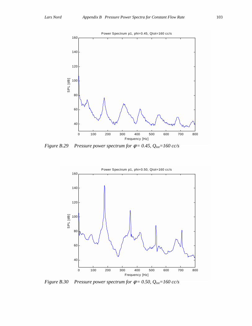
Lars Nord Appendix B Pressure Power Spectra for Constant Flow Rate
103
0 100 200 300 400 500 600 700 800
40
60
80
100
120
140
160Power Spectrum p1, phi=0.45, Qtot=160 cc/s
Frequency [Hz]
SP
L [d
B]
Figure B.29 Pressure power spectrum for φ = 0.45, Qtot=160 cc/s
0 100 200 300 400 500 600 700 800
40
60
80
100
120
140
160Power Spectrum p1, phi=0.50, Qtot=160 cc/s
Frequency [Hz]
SP
L [d
B]
Figure B.30 Pressure power spectrum for φ = 0.50, Qtot=160 cc/s

Lars Nord Appendix B Pressure Power Spectra for Constant Flow Rate
104
0 100 200 300 400 500 600 700 800
40
60
80
100
120
140
160Power Spectrum p1, phi=0.60, Qtot=160 cc/s
Frequency [Hz]
SP
L [d
B]
Figure B.31 Pressure power spectrum for φ = 0.60, Qtot=160 cc/s
0 100 200 300 400 500 600 700 800
40
60
80
100
120
140
160Power Spectrum p1, phi=0.70, Qtot=160 cc/s
Frequency [Hz]
SP
L [d
B]
Figure B.32 Pressure power spectrum for φ = 0.70, Qtot=160 cc/s

Lars Nord Appendix B Pressure Power Spectra for Constant Flow Rate
105
0 100 200 300 400 500 600 700 800
40
60
80
100
120
140
160Power Spectrum p1, phi=1.20, Qtot=160 cc/s
Frequency [Hz]
SP
L [d
B]
Figure B.33 Pressure power spectrum for φ = 1.20, Qtot=160 cc/s
0 100 200 300 400 500 600 700 800
40
60
80
100
120
140
160Power Spectrum p1, phi=1.30, Qtot=160 cc/s
Frequency [Hz]
SP
L [d
B]
Figure B.34 Pressure power spectrum for φ = 1.30, Qtot=160 cc/s
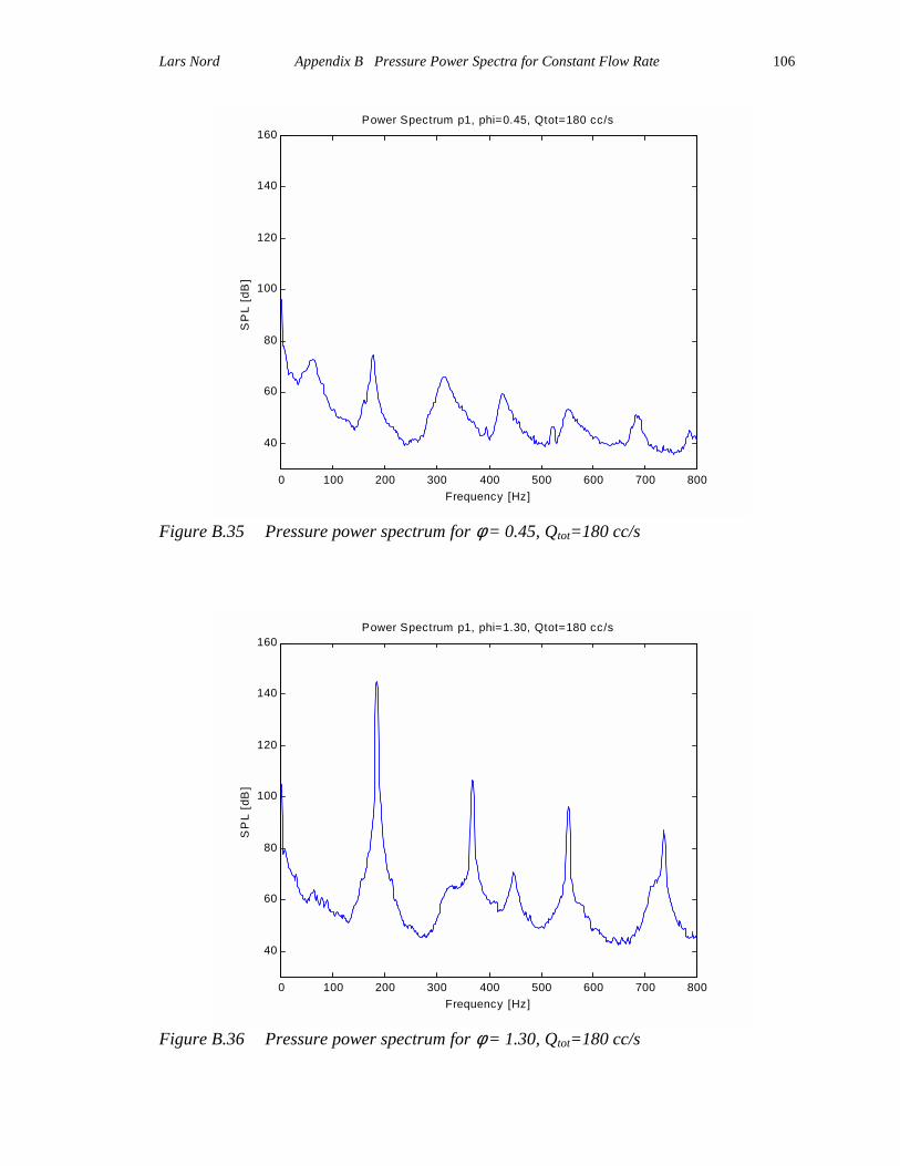
Lars Nord Appendix B Pressure Power Spectra for Constant Flow Rate
106
0 100 200 300 400 500 600 700 800
40
60
80
100
120
140
160Power Spectrum p1, phi=0.45, Qtot=180 cc/s
Frequency [Hz]
SP
L [d
B]
Figure B.35 Pressure power spectrum for φ = 0.45, Qtot=180 cc/s
0 100 200 300 400 500 600 700 800
40
60
80
100
120
140
160Power Spectrum p1, phi=1.30, Qtot=180 cc/s
Frequency [Hz]
SP
L [d
B]
Figure B.36 Pressure power spectrum for φ = 1.30, Qtot=180 cc/s
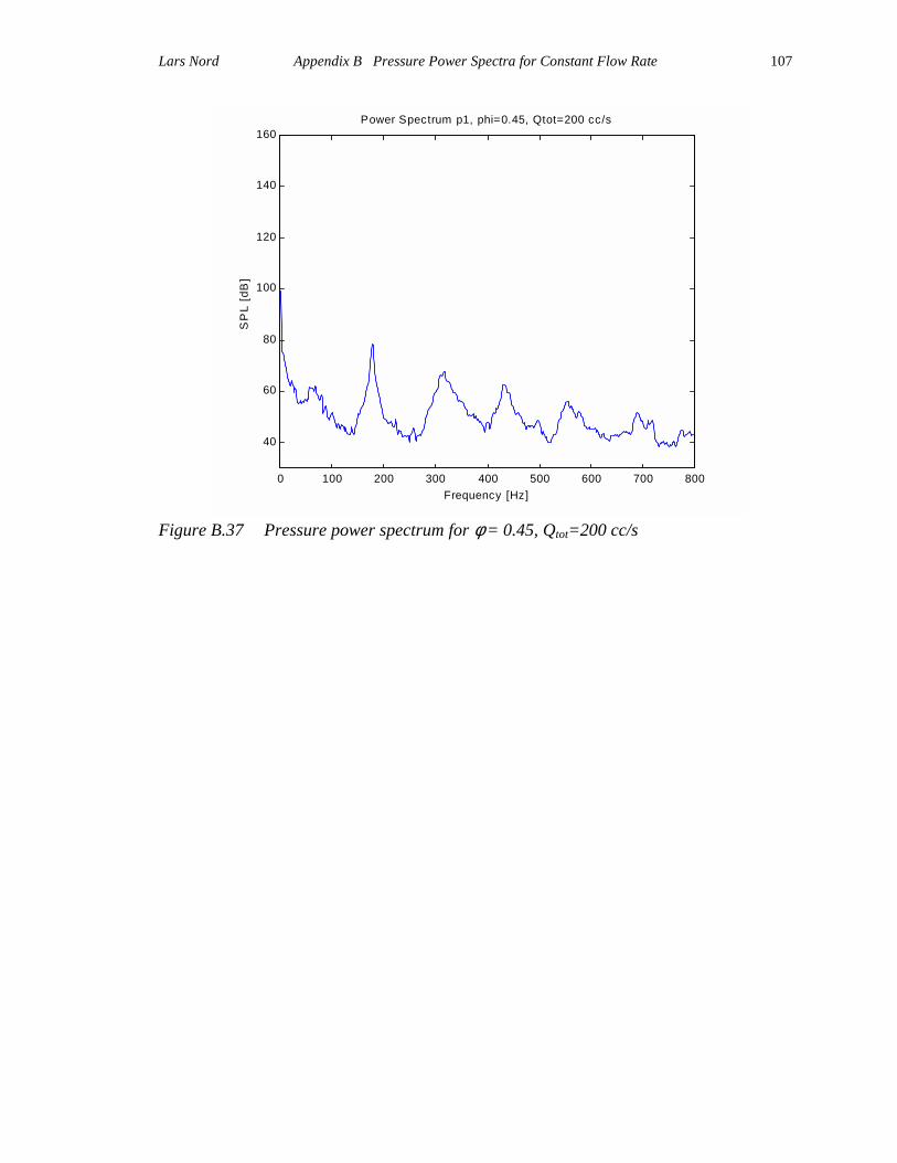
Lars Nord Appendix B Pressure Power Spectra for Constant Flow Rate
107
0 100 200 300 400 500 600 700 800
40
60
80
100
120
140
160Power Spectrum p1, phi=0.45, Qtot=200 cc/s
Frequency [Hz]
SP
L [d
B]
Figure B.37 Pressure power spectrum for φ = 0.45, Qtot=200 cc/s
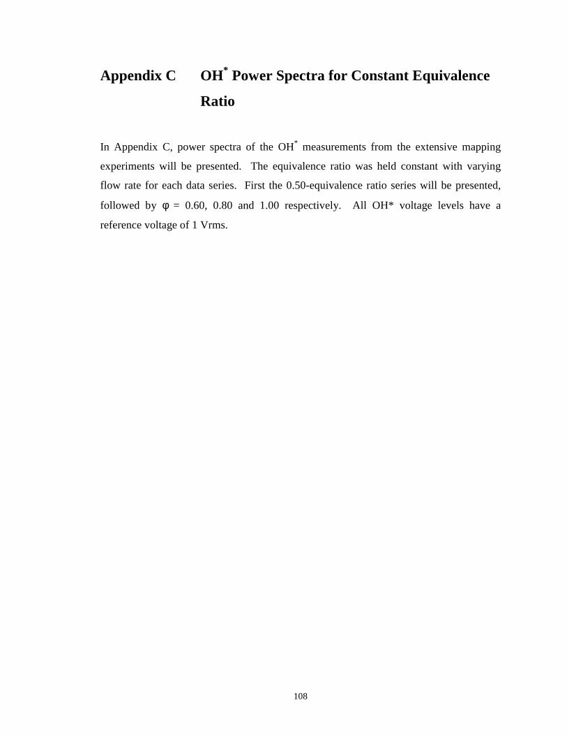
108
Appendix C OH* Power Spectra for Constant Equivalence
Ratio
In Appendix C, power spectra of the OH* measurements from the extensive mapping
experiments will be presented. The equivalence ratio was held constant with varying
flow rate for each data series. First the 0.50-equivalence ratio series will be presented,
followed by φ = 0.60, 0.80 and 1.00 respectively. All OH* voltage levels have a
reference voltage of 1 Vrms.
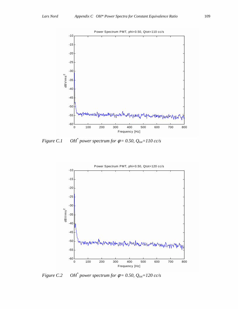
Lars Nord Appendix C OH* Power Spectra for Constant Equivalence Ratio
109
0 100 200 300 400 500 600 700 800-60
-55
-50
-45
-40
-35
-30
-25
-20
-15
-10Power Spectrum PMT, phi=0.50, Qtot=110 cc/s
Frequency [Hz]
dBV
rms2
Figure C.1 OH* power spectrum for φ = 0.50, Qtot=110 cc/s
0 100 200 300 400 500 600 700 800-60
-55
-50
-45
-40
-35
-30
-25
-20
-15
-10Power Spectrum PMT, phi=0.50, Qtot=120 cc/s
Frequency [Hz]
dBV
rms2
Figure C.2 OH* power spectrum for φ = 0.50, Qtot=120 cc/s
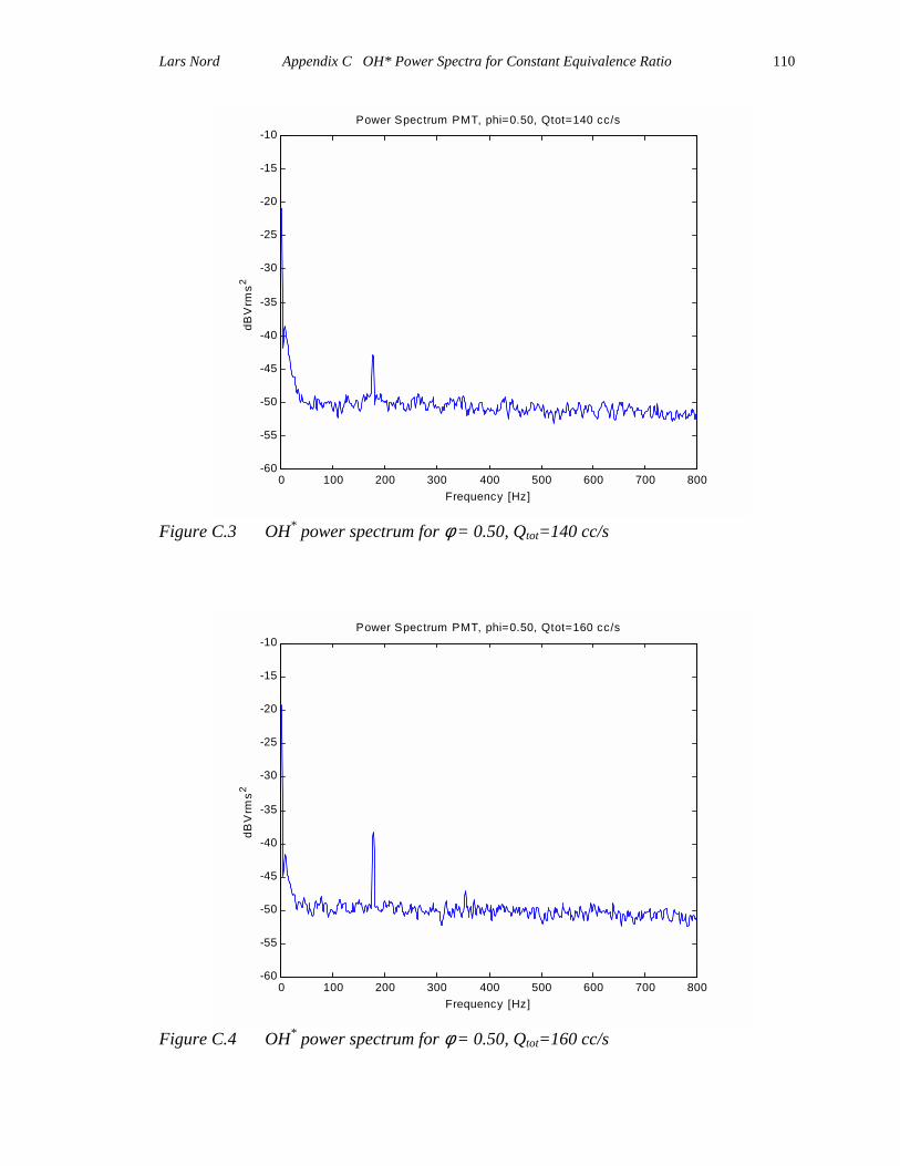
Lars Nord Appendix C OH* Power Spectra for Constant Equivalence Ratio
110
0 100 200 300 400 500 600 700 800-60
-55
-50
-45
-40
-35
-30
-25
-20
-15
-10Power Spectrum PMT, phi=0.50, Qtot=140 cc/s
Frequency [Hz]
dBV
rms2
Figure C.3 OH* power spectrum for φ = 0.50, Qtot=140 cc/s
0 100 200 300 400 500 600 700 800-60
-55
-50
-45
-40
-35
-30
-25
-20
-15
-10Power Spectrum PMT, phi=0.50, Qtot=160 cc/s
Frequency [Hz]
dBV
rms2
Figure C.4 OH* power spectrum for φ = 0.50, Qtot=160 cc/s
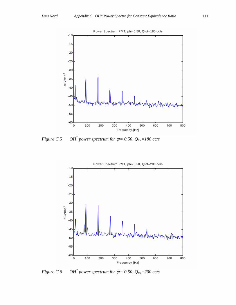
Lars Nord Appendix C OH* Power Spectra for Constant Equivalence Ratio
111
0 100 200 300 400 500 600 700 800-60
-55
-50
-45
-40
-35
-30
-25
-20
-15
-10Power Spectrum PMT, phi=0.50, Qtot=180 cc/s
Frequency [Hz]
dBV
rms2
Figure C.5 OH* power spectrum for φ = 0.50, Qtot=180 cc/s
0 100 200 300 400 500 600 700 800-60
-55
-50
-45
-40
-35
-30
-25
-20
-15
-10Power Spectrum PMT, phi=0.50, Qtot=200 cc/s
Frequency [Hz]
dBV
rms2
Figure C.6 OH* power spectrum for φ = 0.50, Qtot=200 cc/s
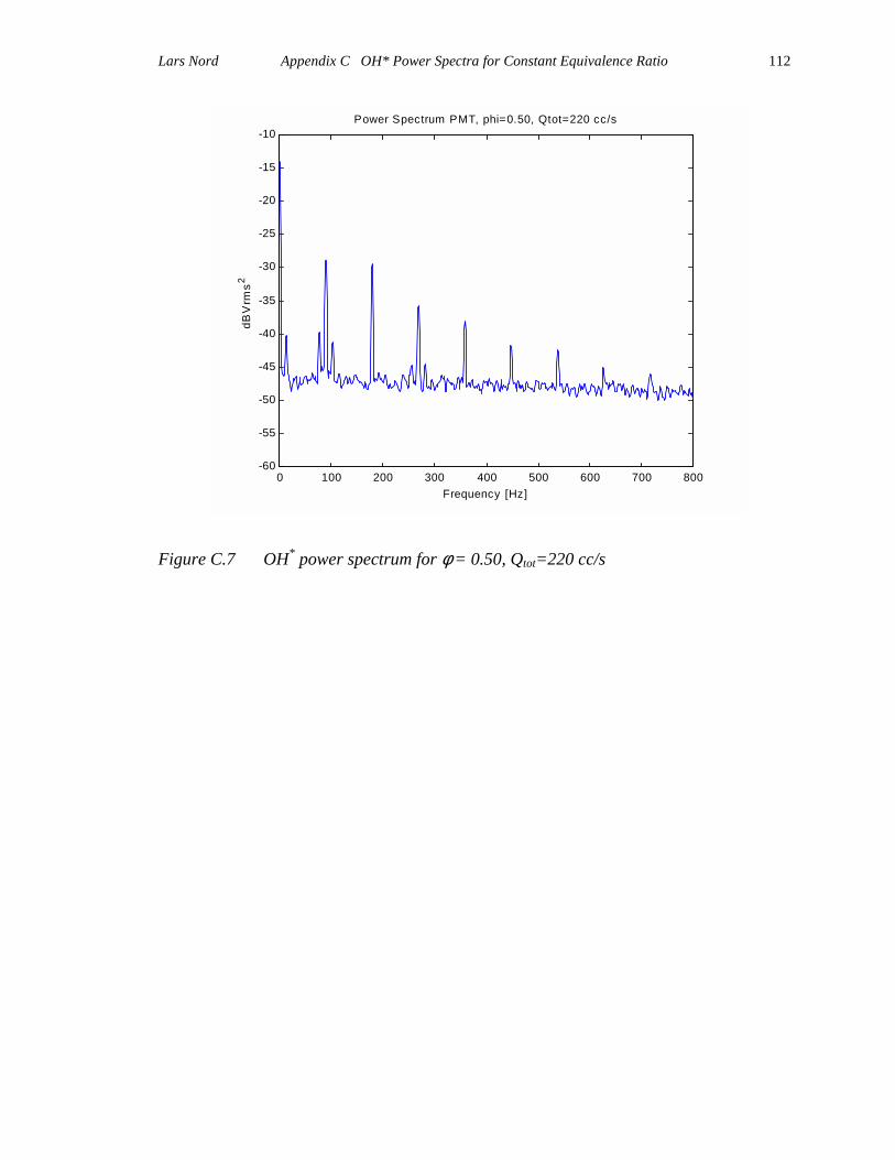
Lars Nord Appendix C OH* Power Spectra for Constant Equivalence Ratio
112
0 100 200 300 400 500 600 700 800-60
-55
-50
-45
-40
-35
-30
-25
-20
-15
-10Power Spectrum PMT, phi=0.50, Qtot=220 cc/s
Frequency [Hz]
dBV
rms2
Figure C.7 OH* power spectrum for φ = 0.50, Qtot=220 cc/s
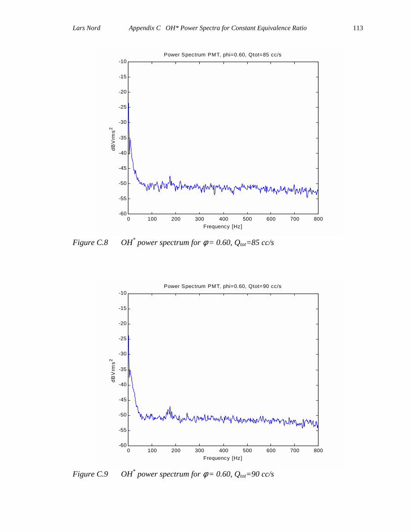
Lars Nord Appendix C OH* Power Spectra for Constant Equivalence Ratio
113
0 100 200 300 400 500 600 700 800-60
-55
-50
-45
-40
-35
-30
-25
-20
-15
-10Power Spectrum PMT, phi=0.60, Qtot=85 cc/s
Frequency [Hz]
dBV
rms2
Figure C.8 OH* power spectrum for φ = 0.60, Qtot=85 cc/s
0 100 200 300 400 500 600 700 800-60
-55
-50
-45
-40
-35
-30
-25
-20
-15
-10Power Spectrum PMT, phi=0.60, Qtot=90 cc/s
Frequency [Hz]
dBV
rms2
Figure C.9 OH* power spectrum for φ = 0.60, Qtot=90 cc/s

Lars Nord Appendix C OH* Power Spectra for Constant Equivalence Ratio
114
0 100 200 300 400 500 600 700 800-60
-55
-50
-45
-40
-35
-30
-25
-20
-15
-10Power Spectrum PMT, phi=0.60, Qtot=95 cc/s
Frequency [Hz]
dBV
rms2
Figure C.10 OH* power spectrum for φ = 0.60, Qtot=95 cc/s
0 100 200 300 400 500 600 700 800-60
-55
-50
-45
-40
-35
-30
-25
-20
-15
-10Power Spectrum PMT, phi=0.60, Qtot=100 cc/s
Frequency [Hz]
dBV
rms2
Figure C.11 OH* power spectrum for φ = 0.60, Qtot=100 cc/s
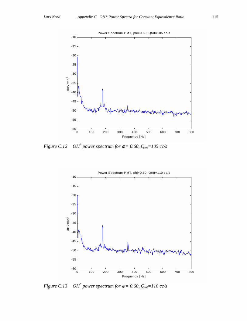
Lars Nord Appendix C OH* Power Spectra for Constant Equivalence Ratio
115
0 100 200 300 400 500 600 700 800-60
-55
-50
-45
-40
-35
-30
-25
-20
-15
-10Power Spectrum PMT, phi=0.60, Qtot=105 cc/s
Frequency [Hz]
dBV
rms2
Figure C.12 OH* power spectrum for φ = 0.60, Qtot=105 cc/s
0 100 200 300 400 500 600 700 800-60
-55
-50
-45
-40
-35
-30
-25
-20
-15
-10Power Spectrum PMT, phi=0.60, Qtot=110 cc/s
Frequency [Hz]
dBV
rms2
Figure C.13 OH* power spectrum for φ = 0.60, Qtot=110 cc/s
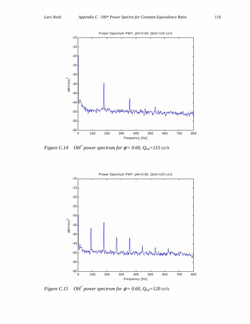
Lars Nord Appendix C OH* Power Spectra for Constant Equivalence Ratio
116
0 100 200 300 400 500 600 700 800-60
-55
-50
-45
-40
-35
-30
-25
-20
-15
-10Power Spectrum PMT, phi=0.60, Qtot=115 cc/s
Frequency [Hz]
dBV
rms2
Figure C.14 OH* power spectrum for φ = 0.60, Qtot=115 cc/s
0 100 200 300 400 500 600 700 800-60
-55
-50
-45
-40
-35
-30
-25
-20
-15
-10Power Spectrum PMT, phi=0.60, Qtot=120 cc/s
Frequency [Hz]
dBV
rms2
Figure C.15 OH* power spectrum for φ = 0.60, Qtot=120 cc/s

Lars Nord Appendix C OH* Power Spectra for Constant Equivalence Ratio
117
0 100 200 300 400 500 600 700 800-60
-55
-50
-45
-40
-35
-30
-25
-20
-15
-10Power Spectrum PMT, phi=0.60, Qtot=125 cc/s
Frequency [Hz]
dBV
rms2
Figure C.16 OH* power spectrum for φ = 0.60, Qtot=125 cc/s
0 100 200 300 400 500 600 700 800-60
-55
-50
-45
-40
-35
-30
-25
-20
-15
-10Power Spectrum PMT, phi=0.60, Qtot=130 cc/s
Frequency [Hz]
dBV
rms2
Figure C.17 OH* power spectrum for φ = 0.60, Qtot=130 cc/s
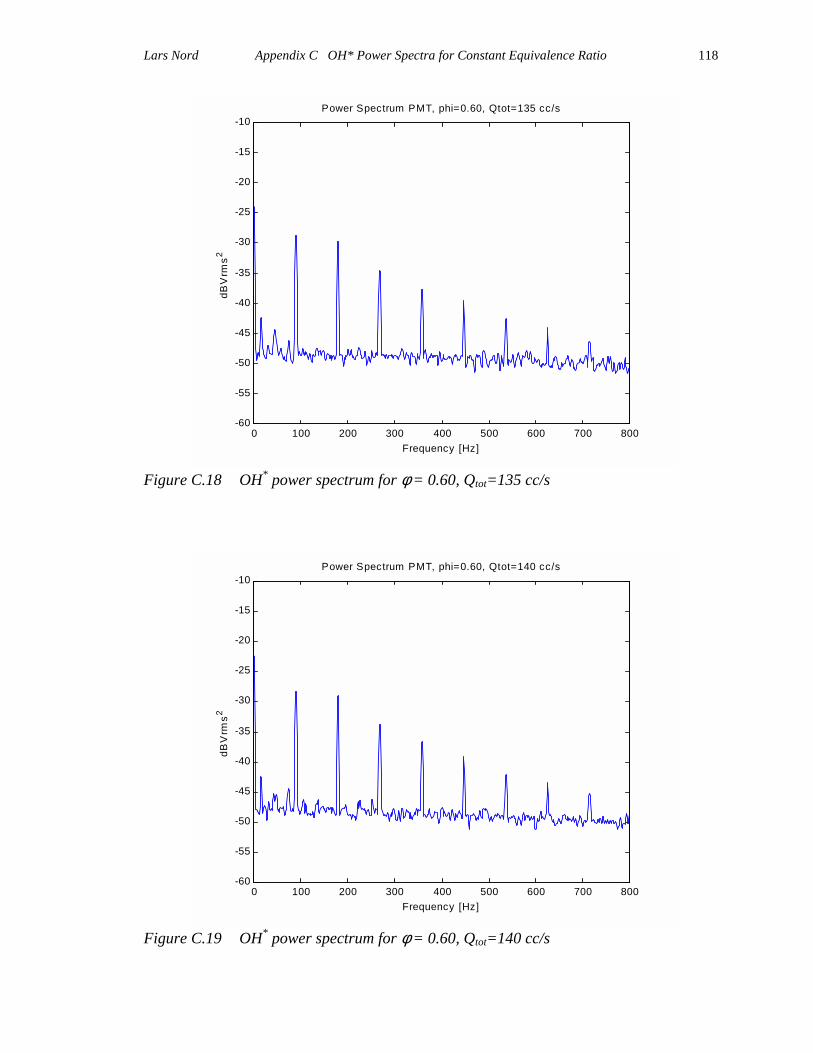
Lars Nord Appendix C OH* Power Spectra for Constant Equivalence Ratio
118
0 100 200 300 400 500 600 700 800-60
-55
-50
-45
-40
-35
-30
-25
-20
-15
-10Power Spectrum PMT, phi=0.60, Qtot=135 cc/s
Frequency [Hz]
dBV
rms2
Figure C.18 OH* power spectrum for φ = 0.60, Qtot=135 cc/s
0 100 200 300 400 500 600 700 800-60
-55
-50
-45
-40
-35
-30
-25
-20
-15
-10Power Spectrum PMT, phi=0.60, Qtot=140 cc/s
Frequency [Hz]
dBV
rms2
Figure C.19 OH* power spectrum for φ = 0.60, Qtot=140 cc/s

Lars Nord Appendix C OH* Power Spectra for Constant Equivalence Ratio
119
0 100 200 300 400 500 600 700 800-60
-55
-50
-45
-40
-35
-30
-25
-20
-15
-10Power Spectrum PMT, phi=0.60, Qtot=145 cc/s
Frequency [Hz]
dBV
rms2
Figure C.20 OH* power spectrum for φ = 0.60, Qtot=145 cc/s
0 100 200 300 400 500 600 700 800-60
-55
-50
-45
-40
-35
-30
-25
-20
-15
-10Power Spectrum PMT, phi=0.60, Qtot=150 cc/s
Frequency [Hz]
dBV
rms2
Figure C.21 OH* power spectrum for φ = 0.60, Qtot=150 cc/s
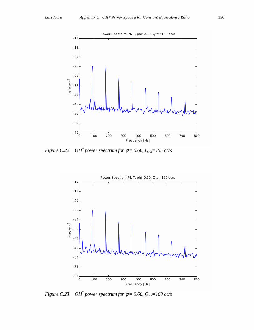
Lars Nord Appendix C OH* Power Spectra for Constant Equivalence Ratio
120
0 100 200 300 400 500 600 700 800-60
-55
-50
-45
-40
-35
-30
-25
-20
-15
-10Power Spectrum PMT, phi=0.60, Qtot=155 cc/s
Frequency [Hz]
dBV
rms2
Figure C.22 OH* power spectrum for φ = 0.60, Qtot=155 cc/s
0 100 200 300 400 500 600 700 800-60
-55
-50
-45
-40
-35
-30
-25
-20
-15
-10Power Spectrum PMT, phi=0.60, Qtot=160 cc/s
Frequency [Hz]
dBV
rms2
Figure C.23 OH* power spectrum for φ = 0.60, Qtot=160 cc/s
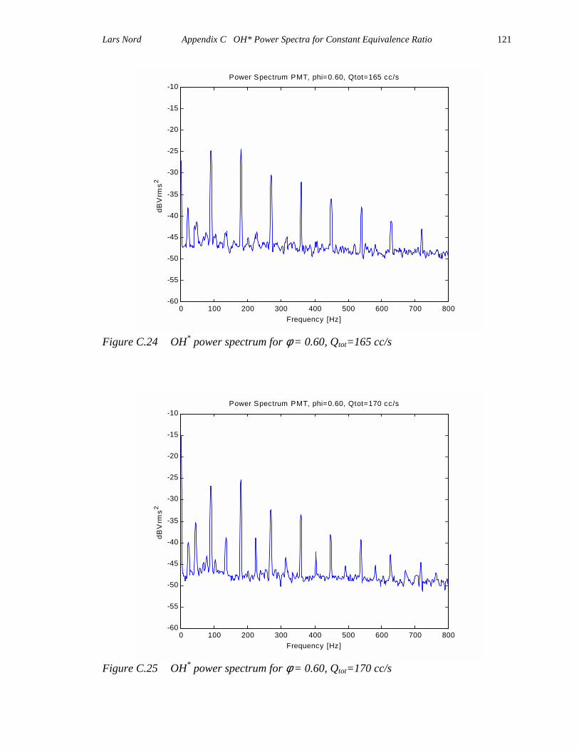
Lars Nord Appendix C OH* Power Spectra for Constant Equivalence Ratio
121
0 100 200 300 400 500 600 700 800-60
-55
-50
-45
-40
-35
-30
-25
-20
-15
-10Power Spectrum PMT, phi=0.60, Qtot=165 cc/s
Frequency [Hz]
dBV
rms2
Figure C.24 OH* power spectrum for φ = 0.60, Qtot=165 cc/s
0 100 200 300 400 500 600 700 800-60
-55
-50
-45
-40
-35
-30
-25
-20
-15
-10Power Spectrum PMT, phi=0.60, Qtot=170 cc/s
Frequency [Hz]
dBV
rms2
Figure C.25 OH* power spectrum for φ = 0.60, Qtot=170 cc/s
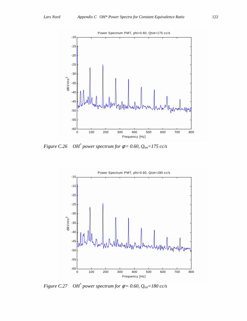
Lars Nord Appendix C OH* Power Spectra for Constant Equivalence Ratio
122
0 100 200 300 400 500 600 700 800-60
-55
-50
-45
-40
-35
-30
-25
-20
-15
-10Power Spectrum PMT, phi=0.60, Qtot=175 cc/s
Frequency [Hz]
dBV
rms2
Figure C.26 OH* power spectrum for φ = 0.60, Qtot=175 cc/s
0 100 200 300 400 500 600 700 800-60
-55
-50
-45
-40
-35
-30
-25
-20
-15
-10Power Spectrum PMT, phi=0.60, Qtot=180 cc/s
Frequency [Hz]
dBV
rms2
Figure C.27 OH* power spectrum for φ = 0.60, Qtot=180 cc/s
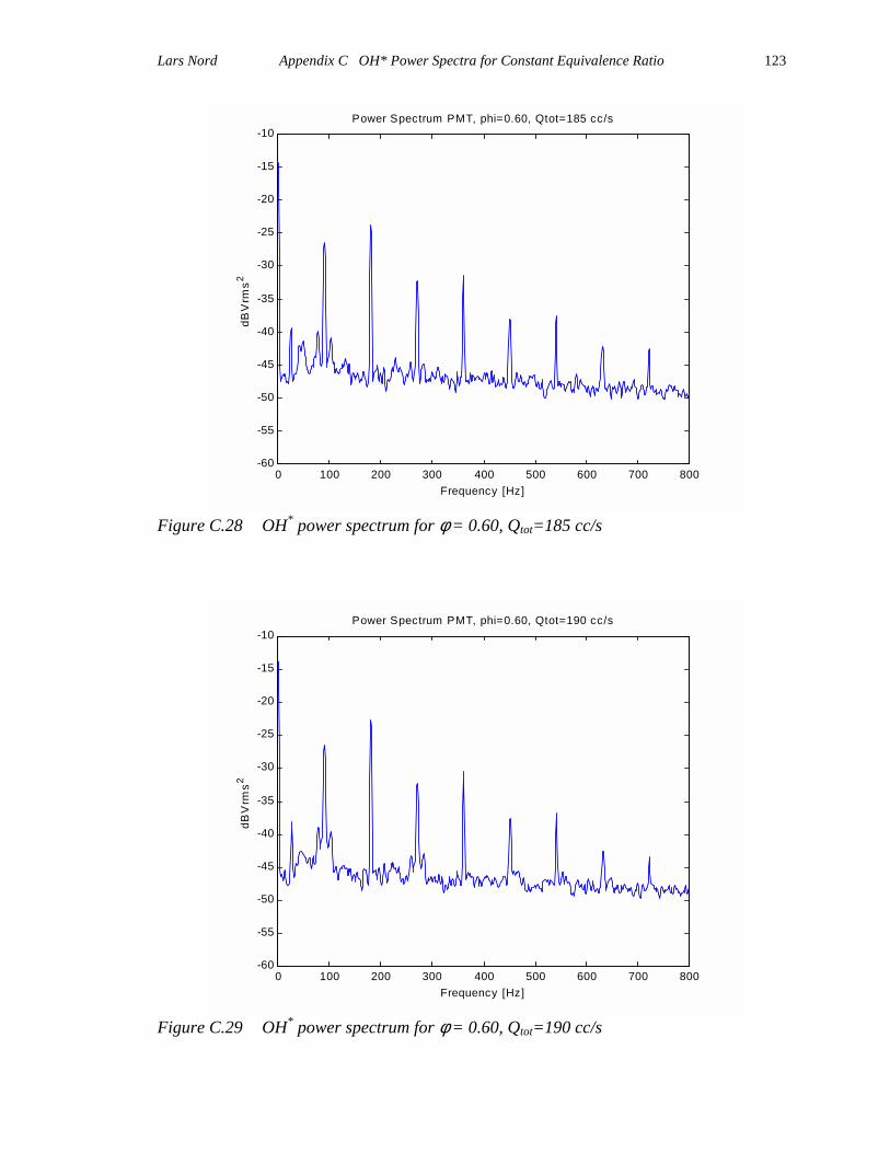
Lars Nord Appendix C OH* Power Spectra for Constant Equivalence Ratio
123
0 100 200 300 400 500 600 700 800-60
-55
-50
-45
-40
-35
-30
-25
-20
-15
-10Power Spectrum PMT, phi=0.60, Qtot=185 cc/s
Frequency [Hz]
dBV
rms2
Figure C.28 OH* power spectrum for φ = 0.60, Qtot=185 cc/s
0 100 200 300 400 500 600 700 800-60
-55
-50
-45
-40
-35
-30
-25
-20
-15
-10Power Spectrum PMT, phi=0.60, Qtot=190 cc/s
Frequency [Hz]
dBV
rms2
Figure C.29 OH* power spectrum for φ = 0.60, Qtot=190 cc/s
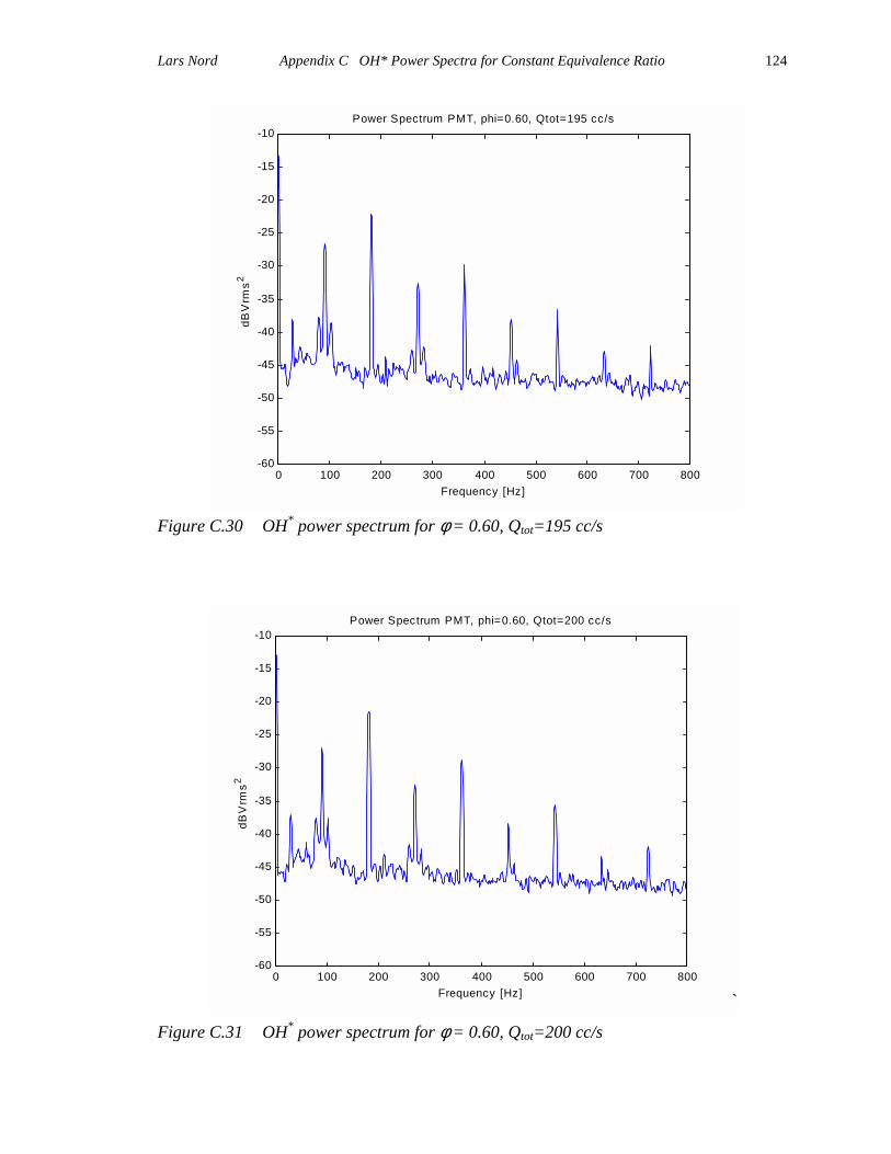
Lars Nord Appendix C OH* Power Spectra for Constant Equivalence Ratio
124
0 100 200 300 400 500 600 700 800-60
-55
-50
-45
-40
-35
-30
-25
-20
-15
-10Power Spectrum PMT, phi=0.60, Qtot=195 cc/s
Frequency [Hz]
dBV
rms2
Figure C.30 OH* power spectrum for φ = 0.60, Qtot=195 cc/s
0 100 200 300 400 500 600 700 800-60
-55
-50
-45
-40
-35
-30
-25
-20
-15
-10Power Spectrum PMT, phi=0.60, Qtot=200 cc/s
Frequency [Hz]
dBV
rms2
`
Figure C.31 OH* power spectrum for φ = 0.60, Qtot=200 cc/s
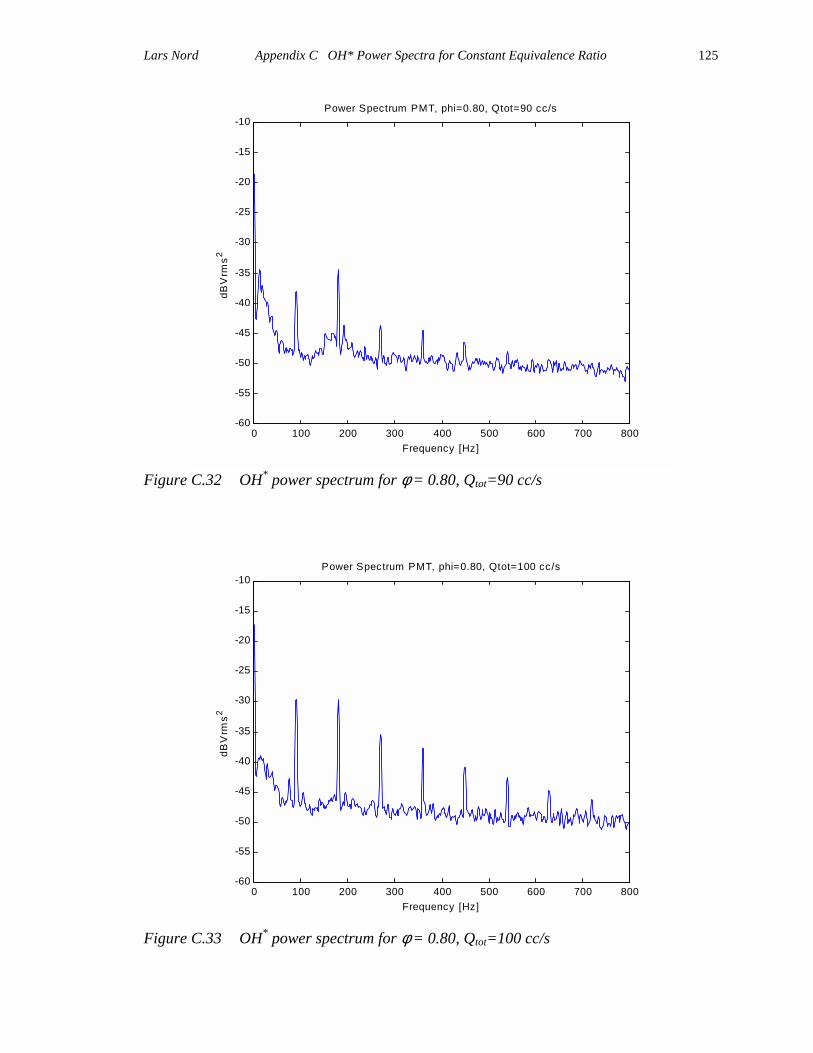
Lars Nord Appendix C OH* Power Spectra for Constant Equivalence Ratio
125
0 100 200 300 400 500 600 700 800-60
-55
-50
-45
-40
-35
-30
-25
-20
-15
-10Power Spectrum PMT, phi=0.80, Qtot=90 cc/s
Frequency [Hz]
dBV
rms2
Figure C.32 OH* power spectrum for φ = 0.80, Qtot=90 cc/s
0 100 200 300 400 500 600 700 800-60
-55
-50
-45
-40
-35
-30
-25
-20
-15
-10Power Spectrum PMT, phi=0.80, Qtot=100 cc/s
Frequency [Hz]
dBV
rms2
Figure C.33 OH* power spectrum for φ = 0.80, Qtot=100 cc/s
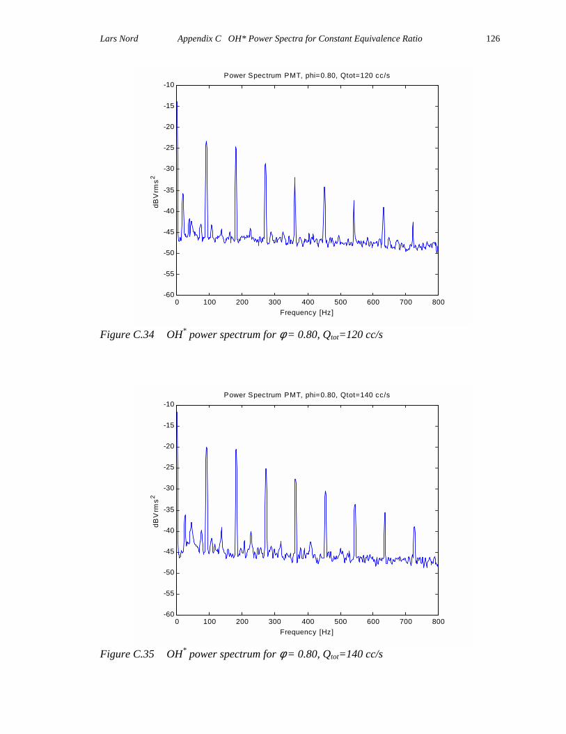
Lars Nord Appendix C OH* Power Spectra for Constant Equivalence Ratio
126
0 100 200 300 400 500 600 700 800-60
-55
-50
-45
-40
-35
-30
-25
-20
-15
-10Power Spectrum PMT, phi=0.80, Qtot=120 cc/s
Frequency [Hz]
dBV
rms2
Figure C.34 OH* power spectrum for φ = 0.80, Qtot=120 cc/s
0 100 200 300 400 500 600 700 800-60
-55
-50
-45
-40
-35
-30
-25
-20
-15
-10Power Spectrum PMT, phi=0.80, Qtot=140 cc/s
Frequency [Hz]
dBV
rms2
Figure C.35 OH* power spectrum for φ = 0.80, Qtot=140 cc/s
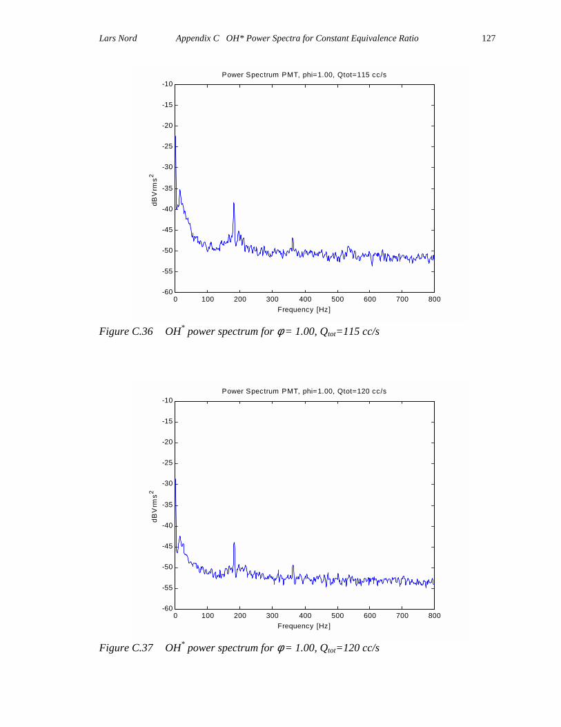
Lars Nord Appendix C OH* Power Spectra for Constant Equivalence Ratio
127
0 100 200 300 400 500 600 700 800-60
-55
-50
-45
-40
-35
-30
-25
-20
-15
-10Power Spectrum PMT, phi=1.00, Qtot=115 cc/s
Frequency [Hz]
dBV
rms2
Figure C.36 OH* power spectrum for φ = 1.00, Qtot=115 cc/s
0 100 200 300 400 500 600 700 800-60
-55
-50
-45
-40
-35
-30
-25
-20
-15
-10Power Spectrum PMT, phi=1.00, Qtot=120 cc/s
Frequency [Hz]
dBV
rms2
Figure C.37 OH* power spectrum for φ = 1.00, Qtot=120 cc/s
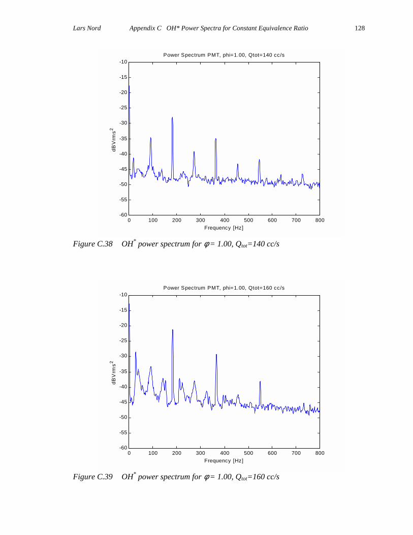
Lars Nord Appendix C OH* Power Spectra for Constant Equivalence Ratio
128
0 100 200 300 400 500 600 700 800-60
-55
-50
-45
-40
-35
-30
-25
-20
-15
-10Power Spectrum PMT, phi=1.00, Qtot=140 cc/s
Frequency [Hz]
dBV
rms2
Figure C.38 OH* power spectrum for φ = 1.00, Qtot=140 cc/s
0 100 200 300 400 500 600 700 800-60
-55
-50
-45
-40
-35
-30
-25
-20
-15
-10Power Spectrum PMT, phi=1.00, Qtot=160 cc/s
Frequency [Hz]
dBV
rms2
Figure C.39 OH* power spectrum for φ = 1.00, Qtot=160 cc/s
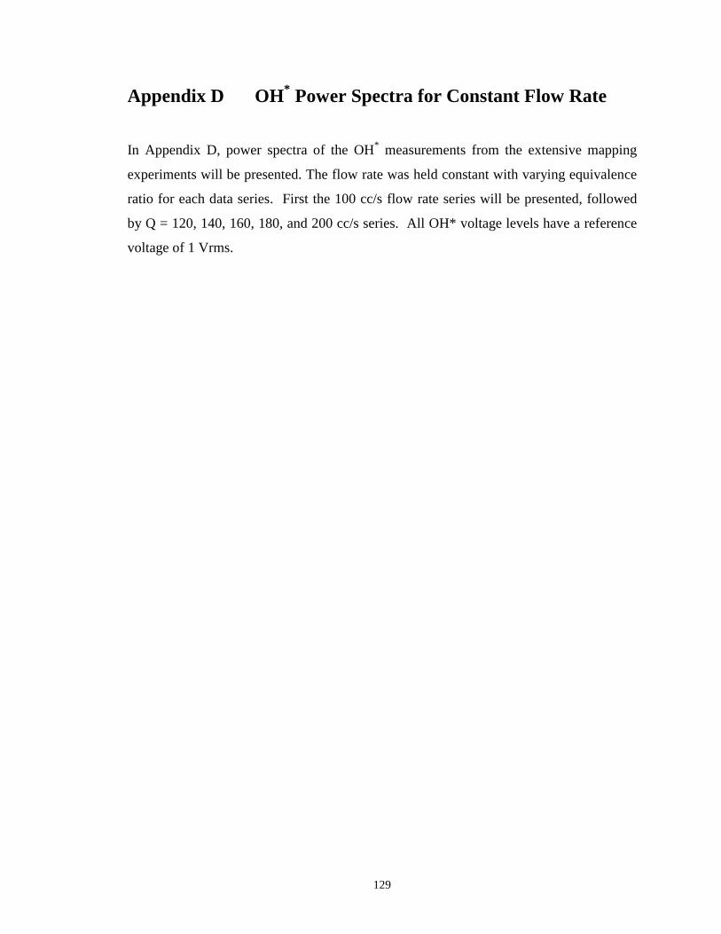
129
Appendix D OH* Power Spectra for Constant Flow Rate
In Appendix D, power spectra of the OH* measurements from the extensive mapping
experiments will be presented. The flow rate was held constant with varying equivalence
ratio for each data series. First the 100 cc/s flow rate series will be presented, followed
by Q = 120, 140, 160, 180, and 200 cc/s series. All OH* voltage levels have a reference
voltage of 1 Vrms.
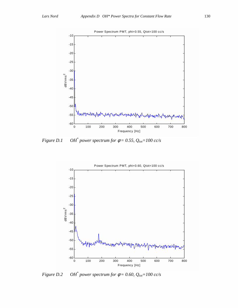
Lars Nord Appendix D OH* Power Spectra for Constant Flow Rate
130
0 100 200 300 400 500 600 700 800-60
-55
-50
-45
-40
-35
-30
-25
-20
-15
-10Power Spectrum PMT, phi=0.55, Qtot=100 cc/s
Frequency [Hz]
dBV
rms2
Figure D.1 OH* power spectrum for φ = 0.55, Qtot=100 cc/s
0 100 200 300 400 500 600 700 800-60
-55
-50
-45
-40
-35
-30
-25
-20
-15
-10Power Spectrum PMT, phi=0.60, Qtot=100 cc/s
Frequency [Hz]
dBV
rms2
Figure D.2 OH* power spectrum for φ = 0.60, Qtot=100 cc/s
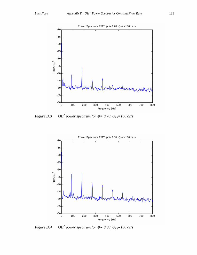
Lars Nord Appendix D OH* Power Spectra for Constant Flow Rate
131
0 100 200 300 400 500 600 700 800-60
-55
-50
-45
-40
-35
-30
-25
-20
-15
-10Power Spectrum PMT, phi=0.70, Qtot=100 cc/s
Frequency [Hz]
dBV
rms2
Figure D.3 OH* power spectrum for φ = 0.70, Qtot=100 cc/s
0 100 200 300 400 500 600 700 800-60
-55
-50
-45
-40
-35
-30
-25
-20
-15
-10Power Spectrum PMT, phi=0.80, Qtot=100 cc/s
Frequency [Hz]
dBV
rms2
Figure D.4 OH* power spectrum for φ = 0.80, Qtot=100 cc/s
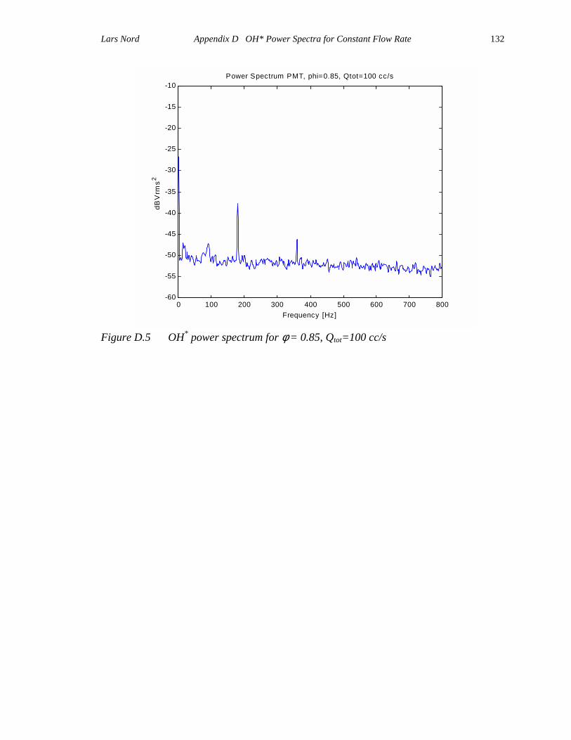
Lars Nord Appendix D OH* Power Spectra for Constant Flow Rate
132
0 100 200 300 400 500 600 700 800-60
-55
-50
-45
-40
-35
-30
-25
-20
-15
-10Power Spectrum PMT, phi=0.85, Qtot=100 cc/s
Frequency [Hz]
dBV
rms2
Figure D.5 OH* power spectrum for φ = 0.85, Qtot=100 cc/s
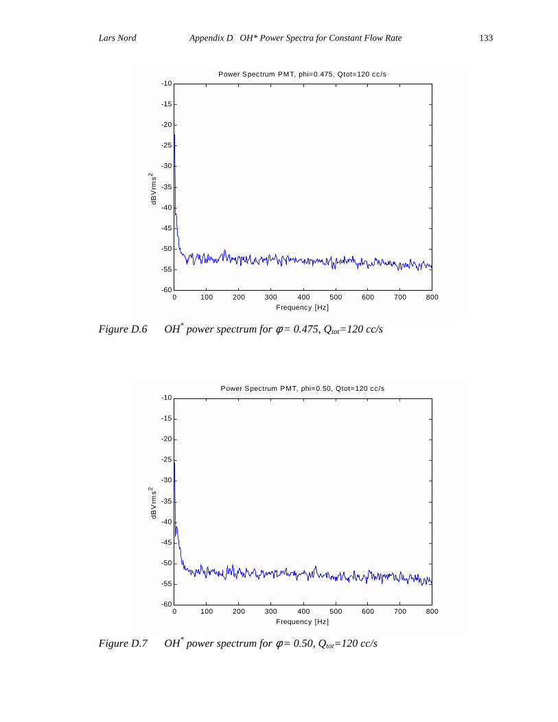
Lars Nord Appendix D OH* Power Spectra for Constant Flow Rate
133
0 100 200 300 400 500 600 700 800-60
-55
-50
-45
-40
-35
-30
-25
-20
-15
-10Power Spectrum PMT, phi=0.475, Qtot=120 cc/s
Frequency [Hz]
dBV
rms2
Figure D.6 OH* power spectrum for φ = 0.475, Qtot=120 cc/s
0 100 200 300 400 500 600 700 800-60
-55
-50
-45
-40
-35
-30
-25
-20
-15
-10Power Spectrum PMT, phi=0.50, Qtot=120 cc/s
Frequency [Hz]
dBV
rms2
Figure D.7 OH* power spectrum for φ = 0.50, Qtot=120 cc/s
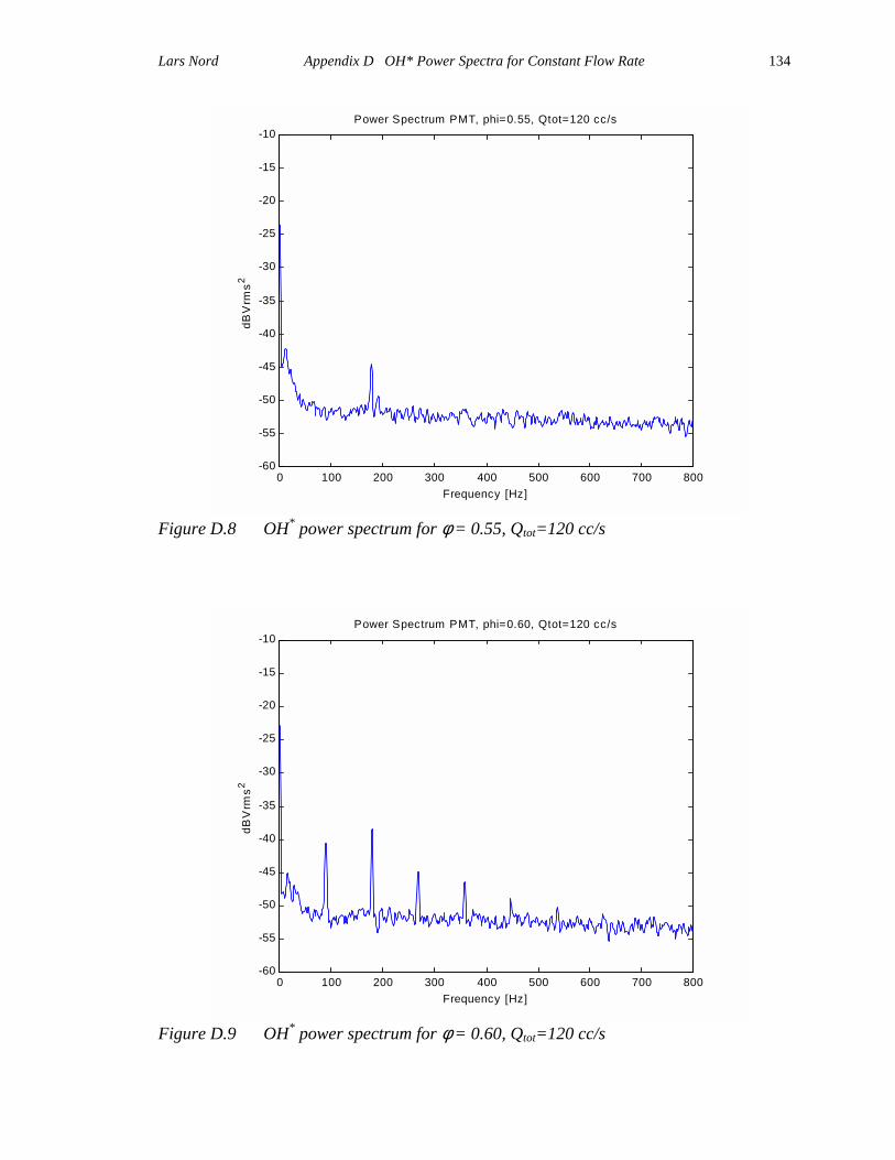
Lars Nord Appendix D OH* Power Spectra for Constant Flow Rate
134
0 100 200 300 400 500 600 700 800-60
-55
-50
-45
-40
-35
-30
-25
-20
-15
-10Power Spectrum PMT, phi=0.55, Qtot=120 cc/s
Frequency [Hz]
dBV
rms2
Figure D.8 OH* power spectrum for φ = 0.55, Qtot=120 cc/s
0 100 200 300 400 500 600 700 800-60
-55
-50
-45
-40
-35
-30
-25
-20
-15
-10Power Spectrum PMT, phi=0.60, Qtot=120 cc/s
Frequency [Hz]
dBV
rms2
Figure D.9 OH* power spectrum for φ = 0.60, Qtot=120 cc/s
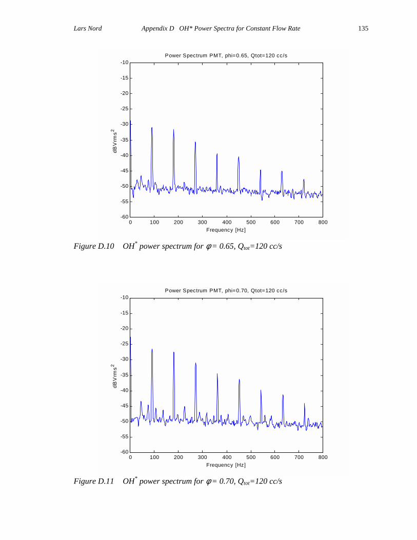
Lars Nord Appendix D OH* Power Spectra for Constant Flow Rate
135
0 100 200 300 400 500 600 700 800-60
-55
-50
-45
-40
-35
-30
-25
-20
-15
-10Power Spectrum PMT, phi=0.65, Qtot=120 cc/s
Frequency [Hz]
dBV
rms2
Figure D.10 OH* power spectrum for φ = 0.65, Qtot=120 cc/s
0 100 200 300 400 500 600 700 800-60
-55
-50
-45
-40
-35
-30
-25
-20
-15
-10Power Spectrum PMT, phi=0.70, Qtot=120 cc/s
Frequency [Hz]
dBV
rms2
Figure D.11 OH* power spectrum for φ = 0.70, Qtot=120 cc/s

Lars Nord Appendix D OH* Power Spectra for Constant Flow Rate
136
0 100 200 300 400 500 600 700 800-60
-55
-50
-45
-40
-35
-30
-25
-20
-15
-10Power Spectrum PMT, phi=0.75, Qtot=120 cc/s
Frequency [Hz]
dBV
rms2
Figure D.12 OH* power spectrum for φ = 0.75, Qtot=120 cc/s
0 100 200 300 400 500 600 700 800-60
-55
-50
-45
-40
-35
-30
-25
-20
-15
-10Power Spectrum PMT, phi=0.80, Qtot=120 cc/s
Frequency [Hz]
dBV
rms2
Figure D.13 OH* power spectrum for φ = 0.80, Qtot=120 cc/s
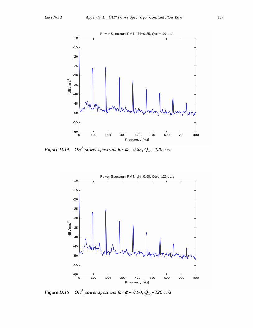
Lars Nord Appendix D OH* Power Spectra for Constant Flow Rate
137
0 100 200 300 400 500 600 700 800-60
-55
-50
-45
-40
-35
-30
-25
-20
-15
-10Power Spectrum PMT, phi=0.85, Qtot=120 cc/s
Frequency [Hz]
dBV
rms2
Figure D.14 OH* power spectrum for φ = 0.85, Qtot=120 cc/s
0 100 200 300 400 500 600 700 800-60
-55
-50
-45
-40
-35
-30
-25
-20
-15
-10Power Spectrum PMT, phi=0.90, Qtot=120 cc/s
Frequency [Hz]
dBV
rms2
Figure D.15 OH* power spectrum for φ = 0.90, Qtot=120 cc/s
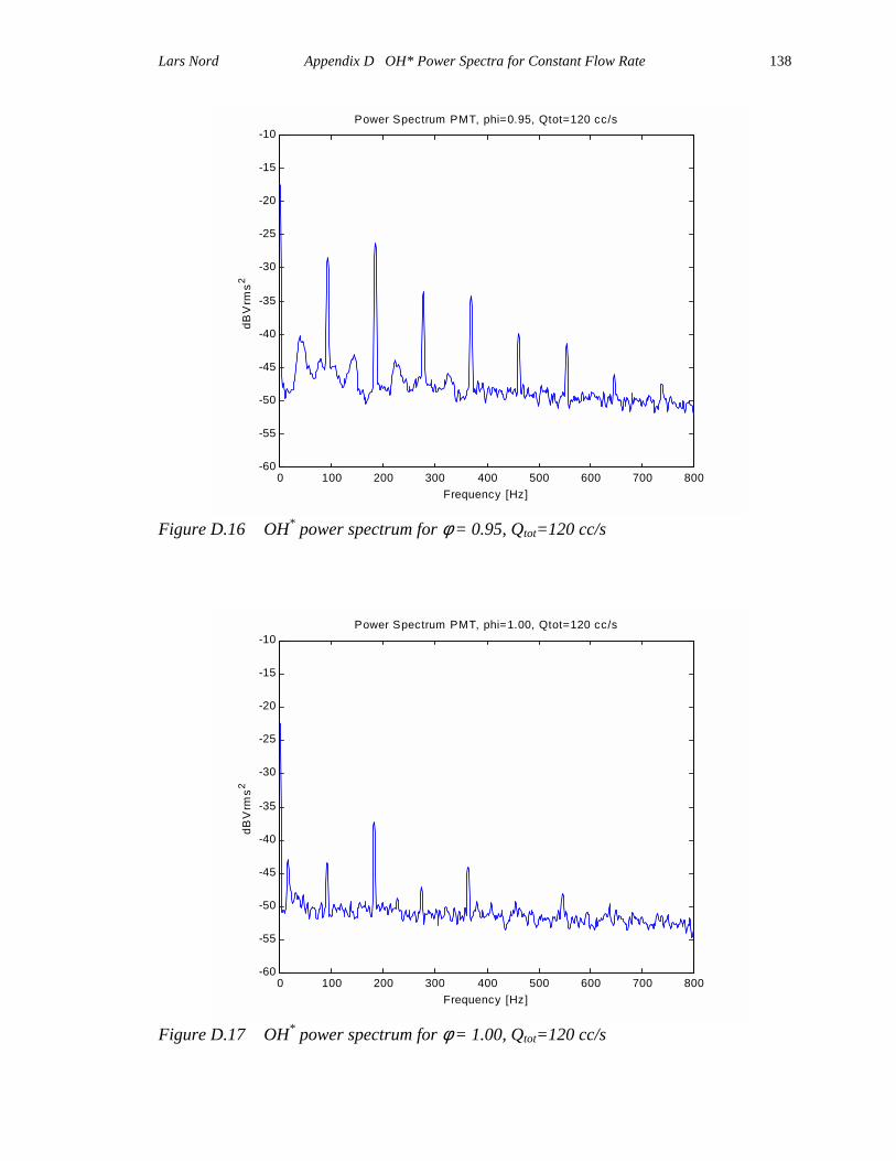
Lars Nord Appendix D OH* Power Spectra for Constant Flow Rate
138
0 100 200 300 400 500 600 700 800-60
-55
-50
-45
-40
-35
-30
-25
-20
-15
-10Power Spectrum PMT, phi=0.95, Qtot=120 cc/s
Frequency [Hz]
dBV
rms2
Figure D.16 OH* power spectrum for φ = 0.95, Qtot=120 cc/s
0 100 200 300 400 500 600 700 800-60
-55
-50
-45
-40
-35
-30
-25
-20
-15
-10Power Spectrum PMT, phi=1.00, Qtot=120 cc/s
Frequency [Hz]
dBV
rms2
Figure D.17 OH* power spectrum for φ = 1.00, Qtot=120 cc/s

Lars Nord Appendix D OH* Power Spectra for Constant Flow Rate
139
0 100 200 300 400 500 600 700 800-60
-55
-50
-45
-40
-35
-30
-25
-20
-15
-10Power Spectrum PMT, phi=1.025, Qtot=120 cc/s
Frequency [Hz]
dBV
rms2
Figure D.18 OH* power spectrum for φ = 1.025, Qtot=120 cc/s
0 100 200 300 400 500 600 700 800-60
-55
-50
-45
-40
-35
-30
-25
-20
-15
-10Power Spectrum PMT, phi=1.04, Qtot=120 cc/s
Frequency [Hz]
dBV
rms2
Figure D.19 OH* power spectrum for φ = 1.04, Qtot=120 cc/s
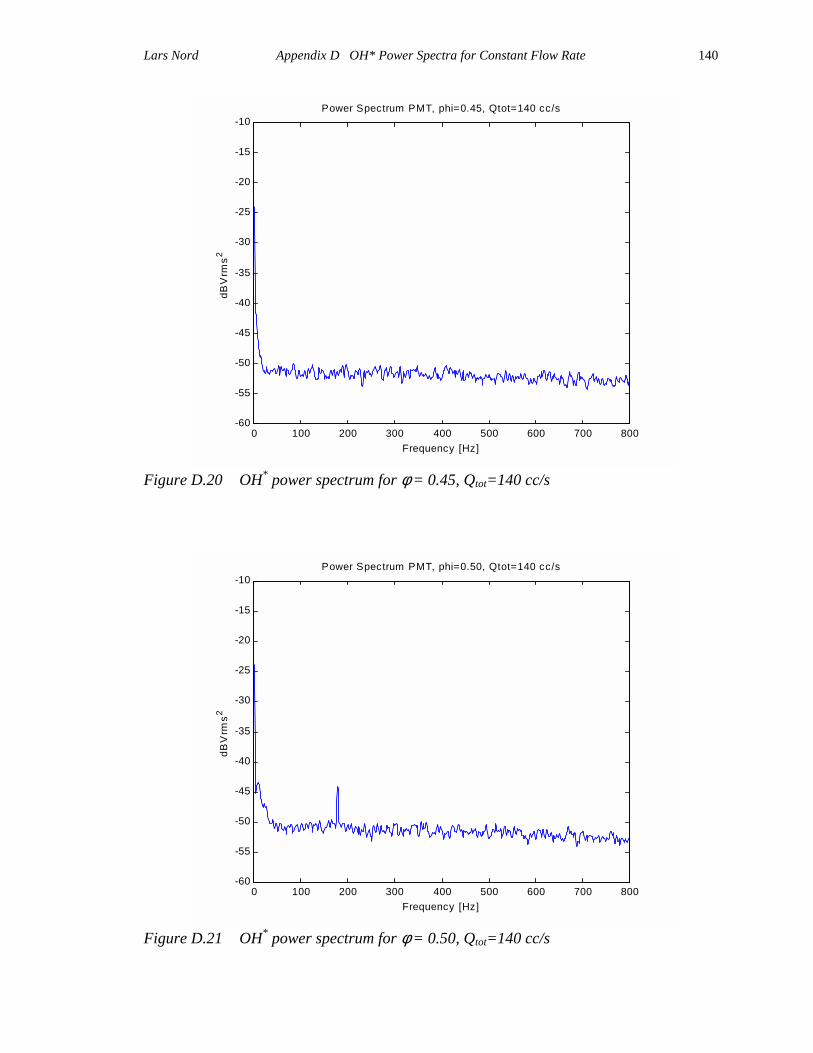
Lars Nord Appendix D OH* Power Spectra for Constant Flow Rate
140
0 100 200 300 400 500 600 700 800-60
-55
-50
-45
-40
-35
-30
-25
-20
-15
-10Power Spectrum PMT, phi=0.45, Qtot=140 cc/s
Frequency [Hz]
dBV
rms2
Figure D.20 OH* power spectrum for φ = 0.45, Qtot=140 cc/s
0 100 200 300 400 500 600 700 800-60
-55
-50
-45
-40
-35
-30
-25
-20
-15
-10Power Spectrum PMT, phi=0.50, Qtot=140 cc/s
Frequency [Hz]
dBV
rms2
Figure D.21 OH* power spectrum for φ = 0.50, Qtot=140 cc/s
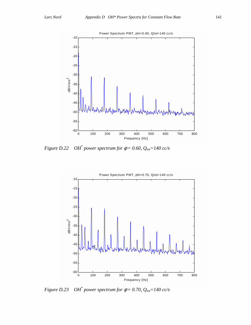
Lars Nord Appendix D OH* Power Spectra for Constant Flow Rate
141
0 100 200 300 400 500 600 700 800-60
-55
-50
-45
-40
-35
-30
-25
-20
-15
-10Power Spectrum PMT, phi=0.60, Qtot=140 cc/s
Frequency [Hz]
dBV
rms2
Figure D.22 OH* power spectrum for φ = 0.60, Qtot=140 cc/s
0 100 200 300 400 500 600 700 800-60
-55
-50
-45
-40
-35
-30
-25
-20
-15
-10Power Spectrum PMT, phi=0.70, Qtot=140 cc/s
Frequency [Hz]
dBV
rms2
Figure D.23 OH* power spectrum for φ = 0.70, Qtot=140 cc/s
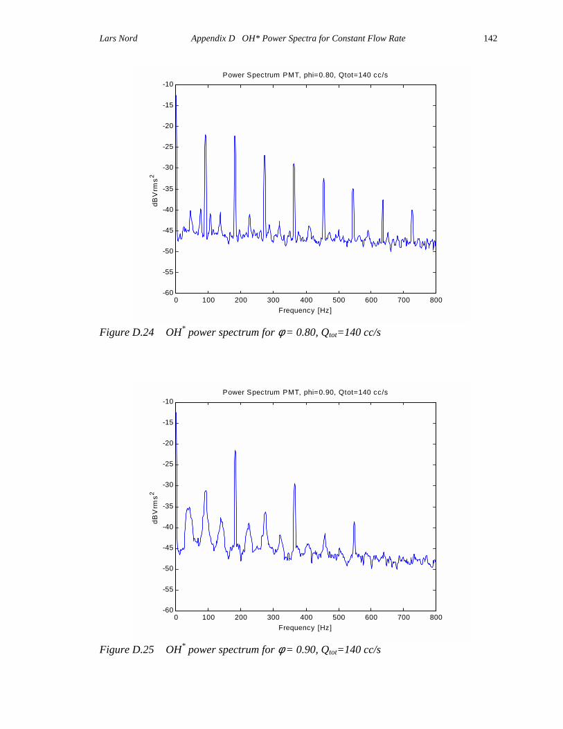
Lars Nord Appendix D OH* Power Spectra for Constant Flow Rate
142
0 100 200 300 400 500 600 700 800-60
-55
-50
-45
-40
-35
-30
-25
-20
-15
-10Power Spectrum PMT, phi=0.80, Qtot=140 cc/s
Frequency [Hz]
dBV
rms2
Figure D.24 OH* power spectrum for φ = 0.80, Qtot=140 cc/s
0 100 200 300 400 500 600 700 800-60
-55
-50
-45
-40
-35
-30
-25
-20
-15
-10Power Spectrum PMT, phi=0.90, Qtot=140 cc/s
Frequency [Hz]
dBV
rms2
Figure D.25 OH* power spectrum for φ = 0.90, Qtot=140 cc/s

Lars Nord Appendix D OH* Power Spectra for Constant Flow Rate
143
0 100 200 300 400 500 600 700 800-60
-55
-50
-45
-40
-35
-30
-25
-20
-15
-10Power Spectrum PMT, phi=1.00, Qtot=140 cc/s
Frequency [Hz]
dBV
rms2
Figure D.26 OH* power spectrum for φ = 1.00, Qtot=140 cc/s
0 100 200 300 400 500 600 700 800-60
-55
-50
-45
-40
-35
-30
-25
-20
-15
-10Power Spectrum PMT, phi=1.10, Qtot=140 cc/s
Frequency [Hz]
dBV
rms2
Figure D.27 OH* power spectrum for φ = 1.10, Qtot=140 cc/s
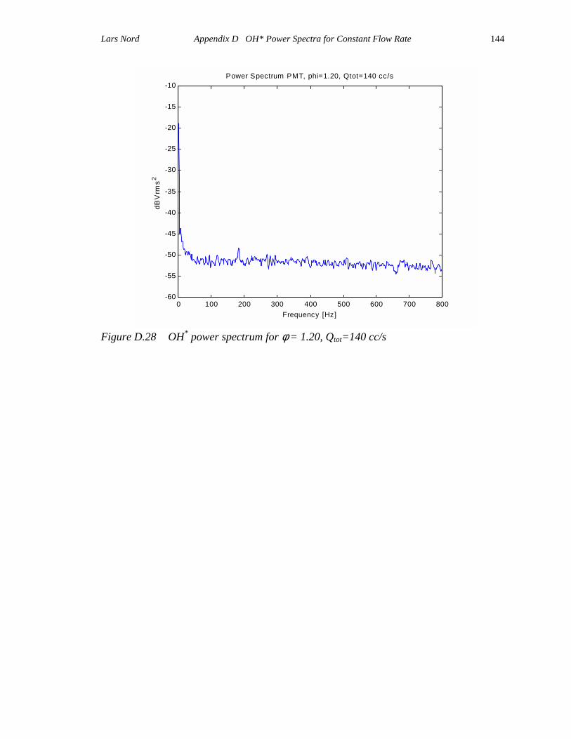
Lars Nord Appendix D OH* Power Spectra for Constant Flow Rate
144
0 100 200 300 400 500 600 700 800-60
-55
-50
-45
-40
-35
-30
-25
-20
-15
-10Power Spectrum PMT, phi=1.20, Qtot=140 cc/s
Frequency [Hz]
dBV
rms2
Figure D.28 OH* power spectrum for φ = 1.20, Qtot=140 cc/s

Lars Nord Appendix D OH* Power Spectra for Constant Flow Rate
145
0 100 200 300 400 500 600 700 800-60
-55
-50
-45
-40
-35
-30
-25
-20
-15
-10Power Spectrum PMT, phi=0.45, Qtot=160 cc/s
Frequency [Hz]
dBV
rms2
Figure D.29 OH* power spectrum for φ = 0.45, Qtot=160 cc/s
0 100 200 300 400 500 600 700 800-60
-55
-50
-45
-40
-35
-30
-25
-20
-15
-10Power Spectrum PMT, phi=0.50, Qtot=160 cc/s
Frequency [Hz]
dBV
rms2
Figure D.30 OH* power spectrum for φ = 0.50, Qtot=160 cc/s
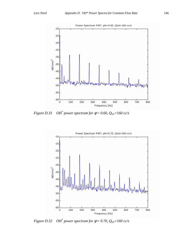
Lars Nord Appendix D OH* Power Spectra for Constant Flow Rate
146
0 100 200 300 400 500 600 700 800-60
-55
-50
-45
-40
-35
-30
-25
-20
-15
-10Power Spectrum PMT, phi=0.60, Qtot=160 cc/s
Frequency [Hz]
dBV
rms2
Figure D.31 OH* power spectrum for φ = 0.60, Qtot=160 cc/s
0 100 200 300 400 500 600 700 800-60
-55
-50
-45
-40
-35
-30
-25
-20
-15
-10Power Spectrum PMT, phi=0.70, Qtot=160 cc/s
Frequency [Hz]
dBV
rms2
Figure D.32 OH* power spectrum for φ = 0.70, Qtot=160 cc/s
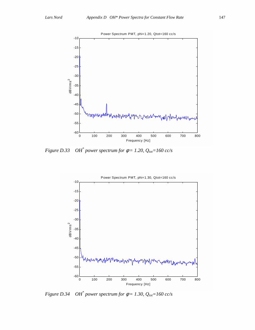
Lars Nord Appendix D OH* Power Spectra for Constant Flow Rate
147
0 100 200 300 400 500 600 700 800-60
-55
-50
-45
-40
-35
-30
-25
-20
-15
-10Power Spectrum PMT, phi=1.20, Qtot=160 cc/s
Frequency [Hz]
dBV
rms2
Figure D.33 OH* power spectrum for φ = 1.20, Qtot=160 cc/s
0 100 200 300 400 500 600 700 800-60
-55
-50
-45
-40
-35
-30
-25
-20
-15
-10Power Spectrum PMT, phi=1.30, Qtot=160 cc/s
Frequency [Hz]
dBV
rms2
Figure D.34 OH* power spectrum for φ = 1.30, Qtot=160 cc/s
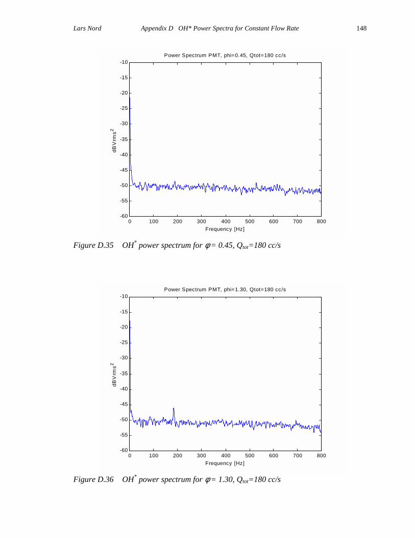
Lars Nord Appendix D OH* Power Spectra for Constant Flow Rate
148
0 100 200 300 400 500 600 700 800-60
-55
-50
-45
-40
-35
-30
-25
-20
-15
-10Power Spectrum PMT, phi=0.45, Qtot=180 cc/s
Frequency [Hz]
dBV
rms2
Figure D.35 OH* power spectrum for φ = 0.45, Qtot=180 cc/s
0 100 200 300 400 500 600 700 800-60
-55
-50
-45
-40
-35
-30
-25
-20
-15
-10Power Spectrum PMT, phi=1.30, Qtot=180 cc/s
Frequency [Hz]
dBV
rms2
Figure D.36 OH* power spectrum for φ = 1.30, Qtot=180 cc/s
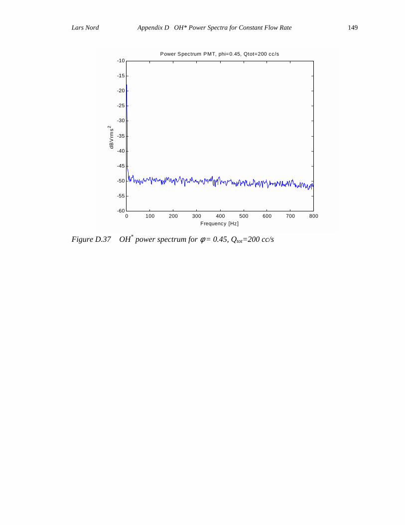
Lars Nord Appendix D OH* Power Spectra for Constant Flow Rate
149
0 100 200 300 400 500 600 700 800-60
-55
-50
-45
-40
-35
-30
-25
-20
-15
-10Power Spectrum PMT, phi=0.45, Qtot=200 cc/s
Frequency [Hz]
dBV
rms2
Figure D.37 OH* power spectrum for φ = 0.45, Qtot=200 cc/s
150
Appendix E Axial Temperature Distribution for Constant
Equivalence Ratio
In Appendix E, axial temperature distributions of the extensive mapping experiments will
be presented. The axial distance is measured from the closed bottom end of the
combustor. The equivalence ratio was held constant with varying flow rate for each data
series. First the 0.50-equivalence ratio series will be presented, followed by φ = 0.60,
0.80 and 1.00 respectively.
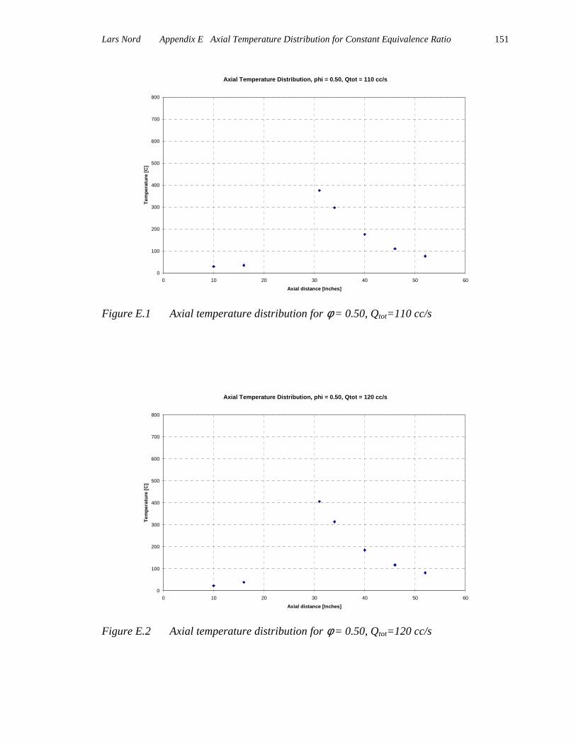
Lars Nord Appendix E Axial Temperature Distribution for Constant Equivalence Ratio
151
Axial Temperature Distribution, phi = 0.50, Qtot = 110 cc/s
0
100
200
300
400
500
600
700
800
0 10 20 30 40 50 60Axial distance [Inches]
Tem
pera
ture
[C]
Figure E.1 Axial temperature distribution for φ = 0.50, Qtot=110 cc/s
Axial Temperature Distribution, phi = 0.50, Qtot = 120 cc/s
0
100
200
300
400
500
600
700
800
0 10 20 30 40 50 60Axial distance [Inches]
Tem
pera
ture
[C]
Figure E.2 Axial temperature distribution for φ = 0.50, Qtot=120 cc/s
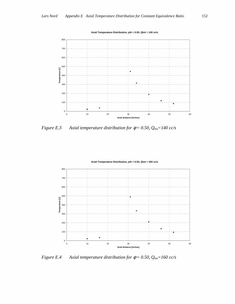
Lars Nord Appendix E Axial Temperature Distribution for Constant Equivalence Ratio
152
Axial Temperature Distribution, phi = 0.50, Qtot = 140 cc/s
0
100
200
300
400
500
600
700
800
0 10 20 30 40 50 60Axial distance [Inches]
Tem
pera
ture
[C]
Figure E.3 Axial temperature distribution for φ = 0.50, Qtot=140 cc/s
Axial Temperature Distribution, phi = 0.50, Qtot = 160 cc/s
0
100
200
300
400
500
600
700
800
0 10 20 30 40 50 60Axial distance [Inches]
Tem
pera
ture
[C]
Figure E.4 Axial temperature distribution for φ = 0.50, Qtot=160 cc/s
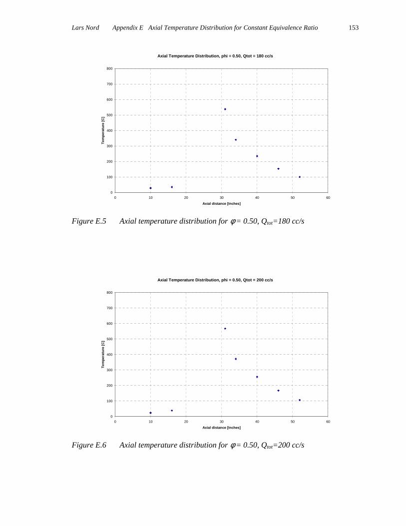
Lars Nord Appendix E Axial Temperature Distribution for Constant Equivalence Ratio
153
Axial Temperature Distribution, phi = 0.50, Qtot = 180 cc/s
0
100
200
300
400
500
600
700
800
0 10 20 30 40 50 60Axial distance [Inches]
Tem
pera
ture
[C]
Figure E.5 Axial temperature distribution for φ = 0.50, Qtot=180 cc/s
Axial Temperature Distribution, phi = 0.50, Qtot = 200 cc/s
0
100
200
300
400
500
600
700
800
0 10 20 30 40 50 60Axial distance [Inches]
Tem
pera
ture
[C]
Figure E.6 Axial temperature distribution for φ = 0.50, Qtot=200 cc/s

Lars Nord Appendix E Axial Temperature Distribution for Constant Equivalence Ratio
154
Axial Temperature Distribution, phi = 0.50, Qtot = 220 cc/s
0
100
200
300
400
500
600
700
800
0 10 20 30 40 50 60Axial distance [Inches]
Tem
pera
ture
[C]
Figure E.7 Axial temperature distribution for φ = 0.50, Qtot=220 cc/s

Lars Nord Appendix E Axial Temperature Distribution for Constant Equivalence Ratio
155
Axial Temperature Distribution, phi = 0.60, Qtot = 85 cc/s
0
100
200
300
400
500
600
700
800
0 10 20 30 40 50 60Axial distance [Inches]
Tem
pera
ture
[C]
Figure E.8 Axial temperature distribution for φ = 0.60, Qtot=85 cc/s
Axial Temperature Distribution, phi = 0.60, Qtot = 90 cc/s
0
100
200
300
400
500
600
700
800
0 10 20 30 40 50 60Axial distance [Inches]
Tem
pera
ture
[C]
Figure E.9 Axial temperature distribution for φ = 0.60, Qtot=90 cc/s

Lars Nord Appendix E Axial Temperature Distribution for Constant Equivalence Ratio
156
Axial Temperature Distribution, phi = 0.60, Qtot = 95 cc/s
0
100
200
300
400
500
600
700
800
0 10 20 30 40 50 60Axial distance [Inches]
Tem
pera
ture
[C]
Figure E.10 Axial temperature distribution for φ = 0.60, Qtot=95 cc/s
Axial Temperature Distribution, phi = 0.60, Qtot = 100 cc/s
0
100
200
300
400
500
600
700
800
0 10 20 30 40 50 60Axial distance [Inches]
Tem
pera
ture
[C]
Figure E.11 Axial temperature distribution for φ = 0.60, Qtot=100 cc/s
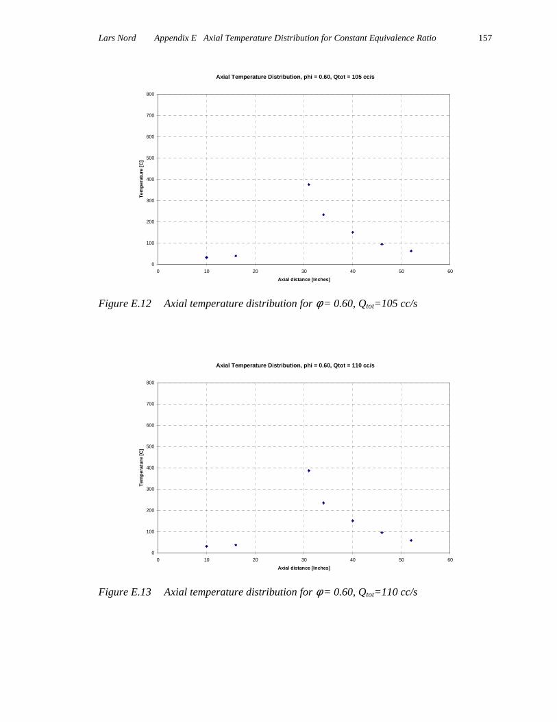
Lars Nord Appendix E Axial Temperature Distribution for Constant Equivalence Ratio
157
Axial Temperature Distribution, phi = 0.60, Qtot = 105 cc/s
0
100
200
300
400
500
600
700
800
0 10 20 30 40 50 60Axial distance [Inches]
Tem
pera
ture
[C]
Figure E.12 Axial temperature distribution for φ = 0.60, Qtot=105 cc/s
Axial Temperature Distribution, phi = 0.60, Qtot = 110 cc/s
0
100
200
300
400
500
600
700
800
0 10 20 30 40 50 60Axial distance [Inches]
Tem
pera
ture
[C]
Figure E.13 Axial temperature distribution for φ = 0.60, Qtot=110 cc/s
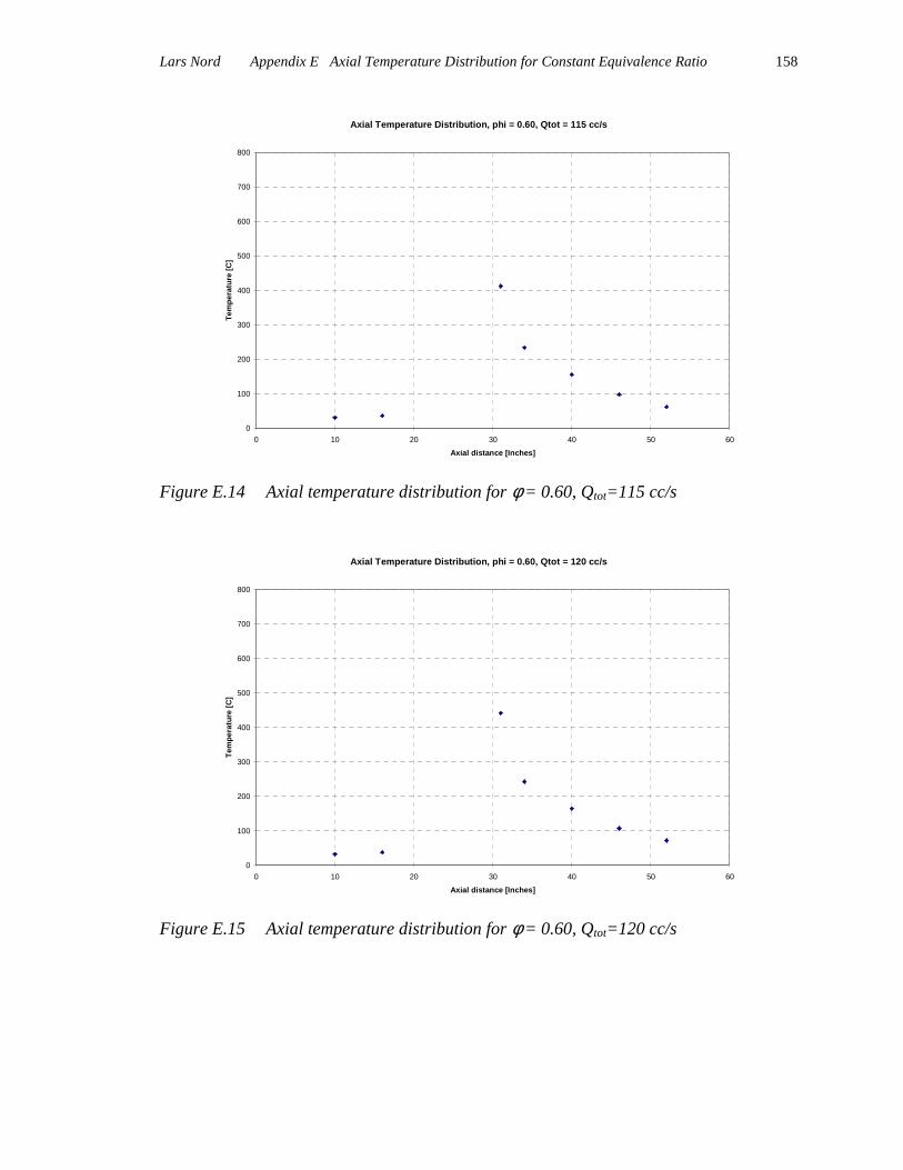
Lars Nord Appendix E Axial Temperature Distribution for Constant Equivalence Ratio
158
Axial Temperature Distribution, phi = 0.60, Qtot = 115 cc/s
0
100
200
300
400
500
600
700
800
0 10 20 30 40 50 60Axial distance [Inches]
Tem
pera
ture
[C]
Figure E.14 Axial temperature distribution for φ = 0.60, Qtot=115 cc/s
Axial Temperature Distribution, phi = 0.60, Qtot = 120 cc/s
0
100
200
300
400
500
600
700
800
0 10 20 30 40 50 60Axial distance [Inches]
Tem
pera
ture
[C]
Figure E.15 Axial temperature distribution for φ = 0.60, Qtot=120 cc/s

Lars Nord Appendix E Axial Temperature Distribution for Constant Equivalence Ratio
159
Axial Temperature Distribution, phi = 0.60, Qtot = 125 cc/s
0
100
200
300
400
500
600
700
800
0 10 20 30 40 50 60Axial distance [Inches]
Tem
pera
ture
[C]
Figure E.16 Axial temperature distribution for φ = 0.60, Qtot=125 cc/s
Axial Temperature Distribution, phi = 0.60, Qtot = 130 cc/s
0
100
200
300
400
500
600
700
800
0 10 20 30 40 50 60Axial distance [Inches]
Tem
pera
ture
[C]
Figure E.17 Axial temperature distribution for φ = 0.60, Qtot=130 cc/s

Lars Nord Appendix E Axial Temperature Distribution for Constant Equivalence Ratio
160
Axial Temperature Distribution, phi = 0.60, Qtot = 135 cc/s
0
100
200
300
400
500
600
700
800
0 10 20 30 40 50 60Axial distance [Inches]
Tem
pera
ture
[C]
Figure E.18 Axial temperature distribution for φ = 0.60, Qtot=135 cc/s
Axial Temperature Distribution, phi = 0.60, Qtot = 140 cc/s
0
100
200
300
400
500
600
700
800
0 10 20 30 40 50 60Axial distance [Inches]
Tem
pera
ture
[C]
Figure E.19 Axial temperature distribution for φ = 0.60, Qtot=140 cc/s
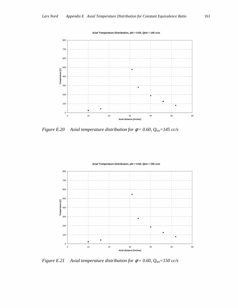
Lars Nord Appendix E Axial Temperature Distribution for Constant Equivalence Ratio
161
Axial Temperature Distribution, phi = 0.60, Qtot = 145 cc/s
0
100
200
300
400
500
600
700
800
0 10 20 30 40 50 60Axial distance [Inches]
Tem
pera
ture
[C]
Figure E.20 Axial temperature distribution for φ = 0.60, Qtot=145 cc/s
Axial Temperature Distribution, phi = 0.60, Qtot = 150 cc/s
0
100
200
300
400
500
600
700
800
0 10 20 30 40 50 60Axial distance [Inches]
Tem
pera
ture
[C]
Figure E.21 Axial temperature distribution for φ = 0.60, Qtot=150 cc/s
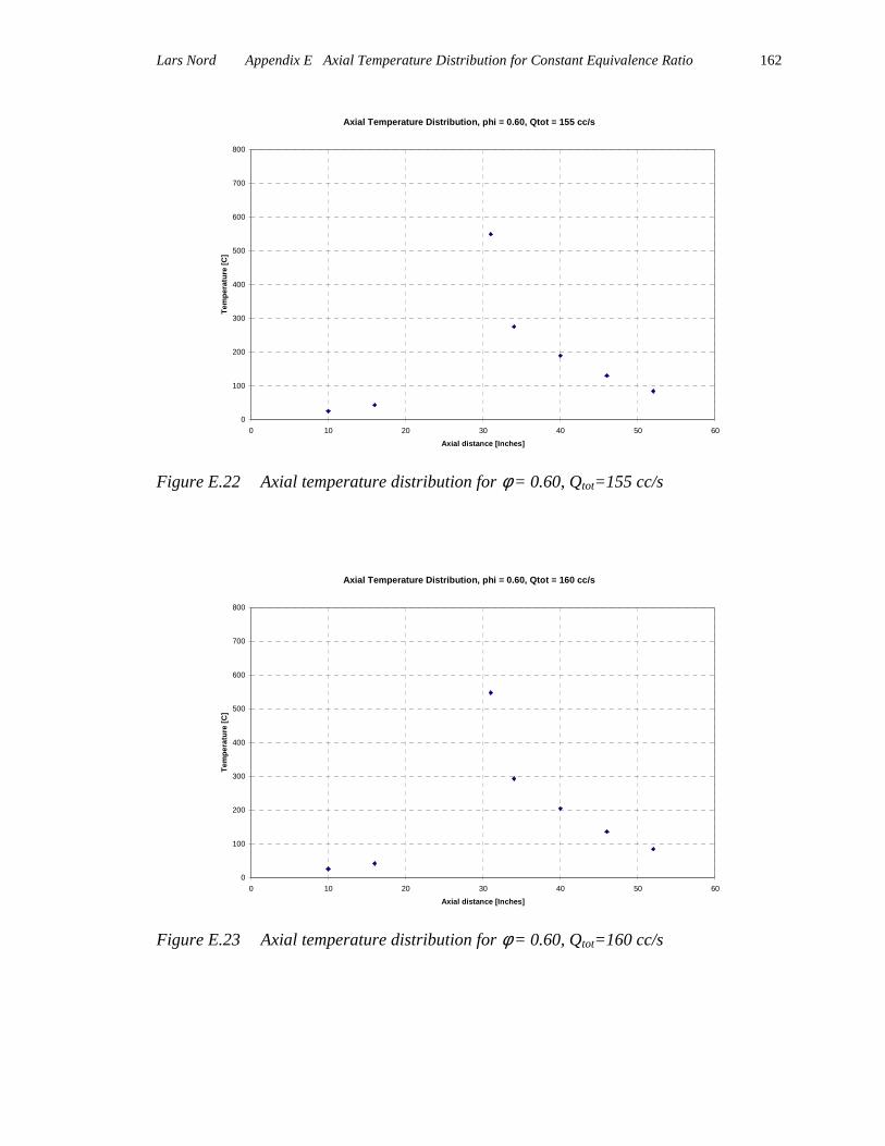
Lars Nord Appendix E Axial Temperature Distribution for Constant Equivalence Ratio
162
Axial Temperature Distribution, phi = 0.60, Qtot = 155 cc/s
0
100
200
300
400
500
600
700
800
0 10 20 30 40 50 60Axial distance [Inches]
Tem
pera
ture
[C]
Figure E.22 Axial temperature distribution for φ = 0.60, Qtot=155 cc/s
Axial Temperature Distribution, phi = 0.60, Qtot = 160 cc/s
0
100
200
300
400
500
600
700
800
0 10 20 30 40 50 60Axial distance [Inches]
Tem
pera
ture
[C]
Figure E.23 Axial temperature distribution for φ = 0.60, Qtot=160 cc/s
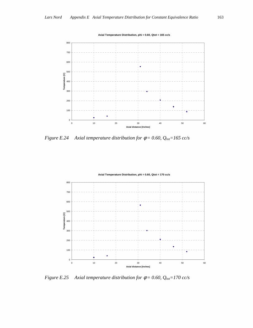
Lars Nord Appendix E Axial Temperature Distribution for Constant Equivalence Ratio
163
Axial Temperature Distribution, phi = 0.60, Qtot = 165 cc/s
0
100
200
300
400
500
600
700
800
0 10 20 30 40 50 60Axial distance [Inches]
Tem
pera
ture
[C]
Figure E.24 Axial temperature distribution for φ = 0.60, Qtot=165 cc/s
Axial Temperature Distribution, phi = 0.60, Qtot = 170 cc/s
0
100
200
300
400
500
600
700
800
0 10 20 30 40 50 60Axial distance [Inches]
Tem
pera
ture
[C]
Figure E.25 Axial temperature distribution for φ = 0.60, Qtot=170 cc/s
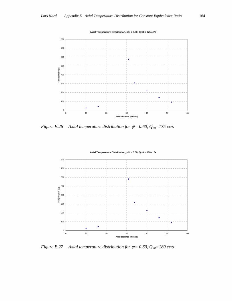
Lars Nord Appendix E Axial Temperature Distribution for Constant Equivalence Ratio
164
Axial Temperature Distribution, phi = 0.60, Qtot = 175 cc/s
0
100
200
300
400
500
600
700
800
0 10 20 30 40 50 60Axial distance [Inches]
Tem
pera
ture
[C]
Figure E.26 Axial temperature distribution for φ = 0.60, Qtot=175 cc/s
Axial Temperature Distribution, phi = 0.60, Qtot = 180 cc/s
0
100
200
300
400
500
600
700
800
0 10 20 30 40 50 60Axial distance [Inches]
Tem
pera
ture
[C]
Figure E.27 Axial temperature distribution for φ = 0.60, Qtot=180 cc/s

Lars Nord Appendix E Axial Temperature Distribution for Constant Equivalence Ratio
165
Axial Temperature Distribution, phi = 0.60, Qtot = 185 cc/s
0
100
200
300
400
500
600
700
800
0 10 20 30 40 50 60Axial distance [Inches]
Tem
pera
ture
[C]
Figure E.28 Axial temperature distribution for φ = 0.60, Qtot=185 cc/s
Axial Temperature Distribution, phi = 0.60, Qtot = 190 cc/s
0
100
200
300
400
500
600
700
800
0 10 20 30 40 50 60Axial distance [Inches]
Tem
pera
ture
[C]
Figure E.29 Axial temperature distribution for φ = 0.60, Qtot=190 cc/s
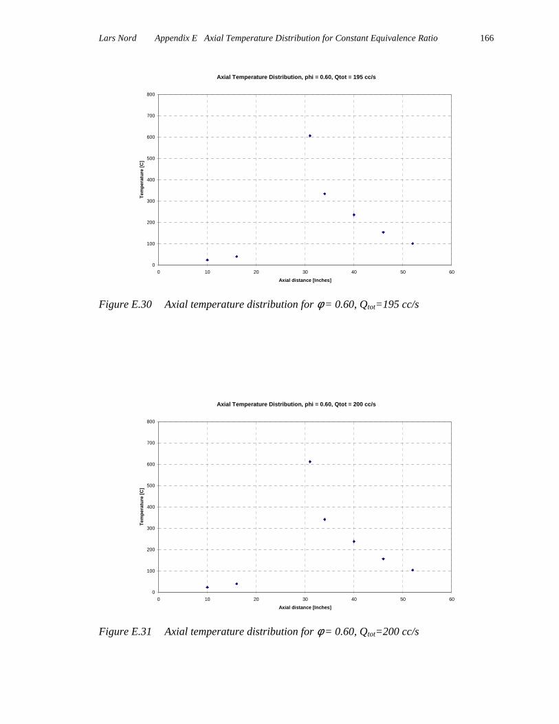
Lars Nord Appendix E Axial Temperature Distribution for Constant Equivalence Ratio
166
Axial Temperature Distribution, phi = 0.60, Qtot = 195 cc/s
0
100
200
300
400
500
600
700
800
0 10 20 30 40 50 60Axial distance [Inches]
Tem
pera
ture
[C]
Figure E.30 Axial temperature distribution for φ = 0.60, Qtot=195 cc/s
Axial Temperature Distribution, phi = 0.60, Qtot = 200 cc/s
0
100
200
300
400
500
600
700
800
0 10 20 30 40 50 60Axial distance [Inches]
Tem
pera
ture
[C]
Figure E.31 Axial temperature distribution for φ = 0.60, Qtot=200 cc/s

Lars Nord Appendix E Axial Temperature Distribution for Constant Equivalence Ratio
167
Axial Temperature Distribution, phi = 0.80, Qtot = 90 cc/s
0
100
200
300
400
500
600
700
800
0 10 20 30 40 50 60Axial distance [Inches]
Tem
pera
ture
[C]
Figure E.32 Axial temperature distribution for φ = 0.80, Qtot=90 cc/s
Axial Temperature Distribution, phi = 0.80, Qtot = 100 cc/s
0
100
200
300
400
500
600
700
800
0 10 20 30 40 50 60Axial distance [Inches]
Tem
pera
ture
[C]
Figure E.33 Axial temperature distribution for φ = 0.80, Qtot=100 cc/s

Lars Nord Appendix E Axial Temperature Distribution for Constant Equivalence Ratio
168
Axial Temperature Distribution, phi = 0.80, Qtot = 120 cc/s
0
100
200
300
400
500
600
700
800
0 10 20 30 40 50 60Axial distance [Inches]
Tem
pera
ture
[C]
Figure E.34 Axial temperature distribution for φ = 0.80, Qtot=120 cc/s
Axial Temperature Distribution, phi = 0.80, Qtot = 140 cc/s
0
100
200
300
400
500
600
700
800
0 10 20 30 40 50 60Axial distance [Inches]
Tem
pera
ture
[C]
Figure E.35 Axial temperature distribution for φ = 0.80, Qtot=140 cc/s

Lars Nord Appendix E Axial Temperature Distribution for Constant Equivalence Ratio
169
Axial Temperature Distribution, phi = 1.00, Qtot = 115 cc/s
0
100
200
300
400
500
600
700
800
0 10 20 30 40 50 60Axial distance [Inches]
Tem
pera
ture
[C]
Figure E.36 Axial temperature distribution for φ = 1.00, Qtot=115 cc/s
Axial Temperature Distribution, phi = 1.00, Qtot = 120 cc/s
0
100
200
300
400
500
600
700
800
0 10 20 30 40 50 60Axial distance [Inches]
Tem
pera
ture
[C]
Figure E.37 Axial temperature distribution for φ = 1.00, Qtot=120 cc/s
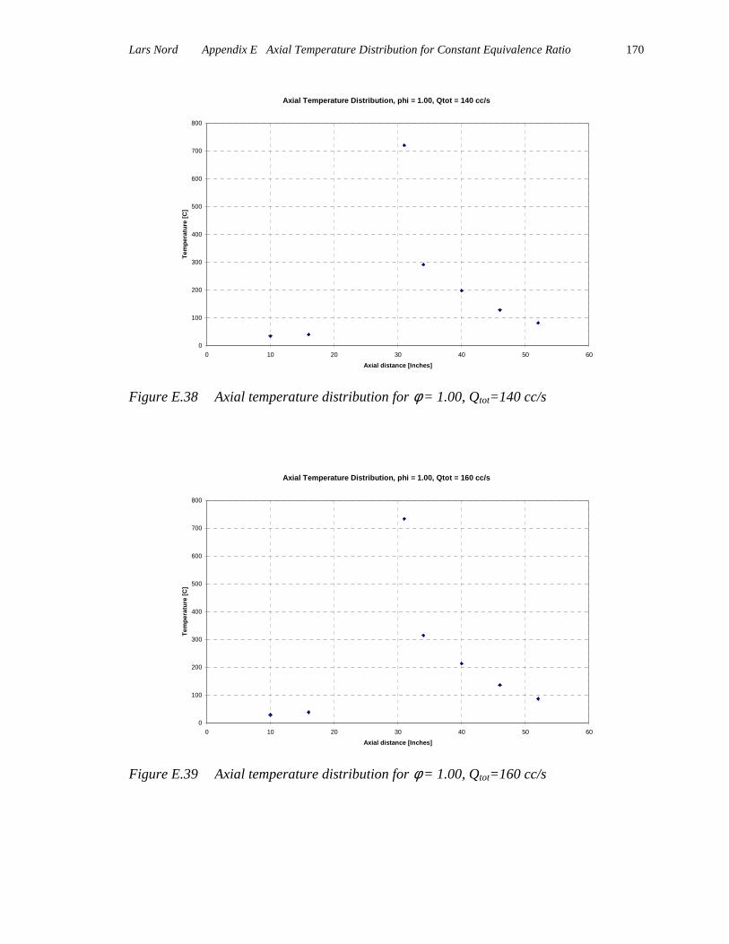
Lars Nord Appendix E Axial Temperature Distribution for Constant Equivalence Ratio
170
Axial Temperature Distribution, phi = 1.00, Qtot = 140 cc/s
0
100
200
300
400
500
600
700
800
0 10 20 30 40 50 60Axial distance [Inches]
Tem
pera
ture
[C]
Figure E.38 Axial temperature distribution for φ = 1.00, Qtot=140 cc/s
Axial Temperature Distribution, phi = 1.00, Qtot = 160 cc/s
0
100
200
300
400
500
600
700
800
0 10 20 30 40 50 60Axial distance [Inches]
Tem
pera
ture
[C]
Figure E.39 Axial temperature distribution for φ = 1.00, Qtot=160 cc/s
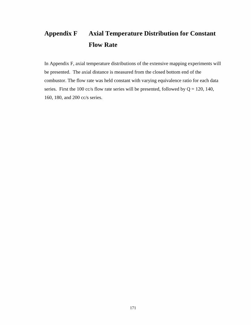
171
Appendix F Axial Temperature Distribution for Constant
Flow Rate
In Appendix F, axial temperature distributions of the extensive mapping experiments will
be presented. The axial distance is measured from the closed bottom end of the
combustor. The flow rate was held constant with varying equivalence ratio for each data
series. First the 100 cc/s flow rate series will be presented, followed by Q = 120, 140,
160, 180, and 200 cc/s series.
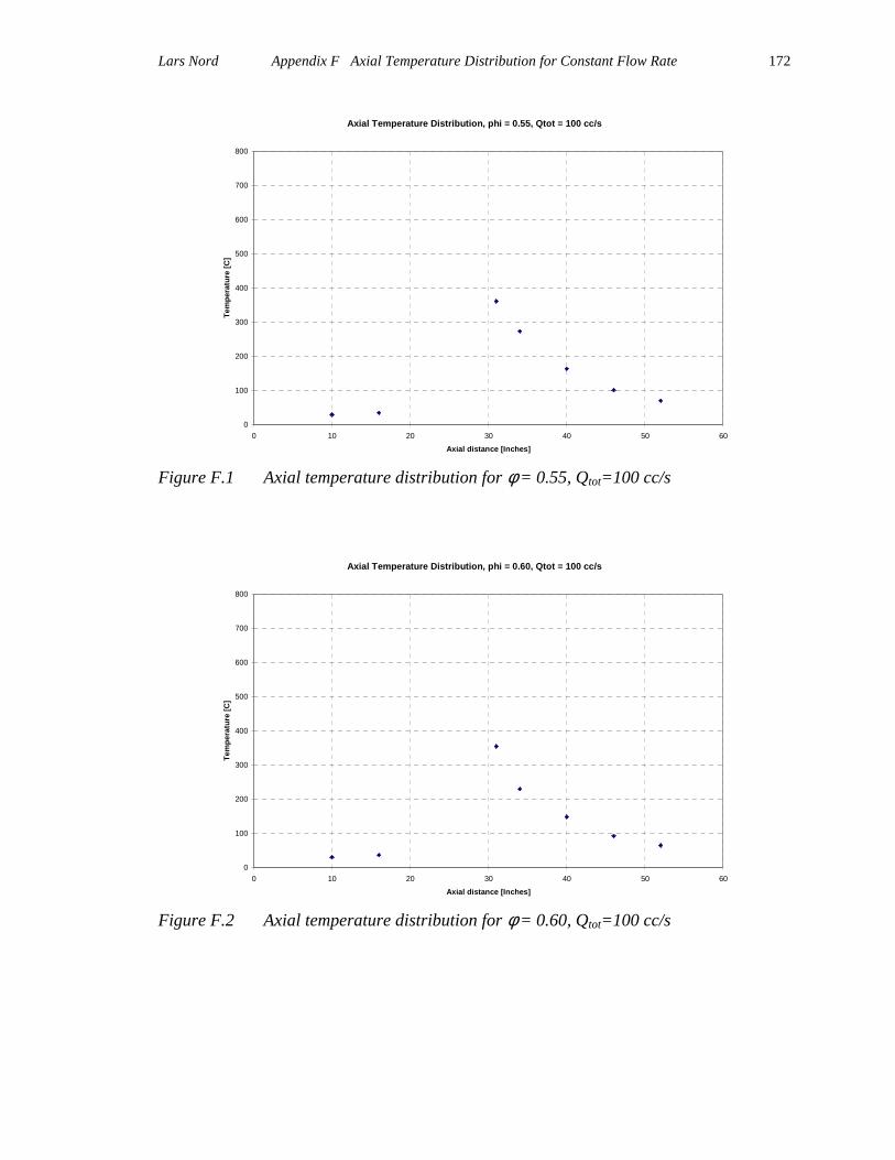
Lars Nord Appendix F Axial Temperature Distribution for Constant Flow Rate
172
Axial Temperature Distribution, phi = 0.55, Qtot = 100 cc/s
0
100
200
300
400
500
600
700
800
0 10 20 30 40 50 60Axial distance [Inches]
Tem
pera
ture
[C]
Figure F.1 Axial temperature distribution for φ = 0.55, Qtot=100 cc/s
Axial Temperature Distribution, phi = 0.60, Qtot = 100 cc/s
0
100
200
300
400
500
600
700
800
0 10 20 30 40 50 60Axial distance [Inches]
Tem
pera
ture
[C]
Figure F.2 Axial temperature distribution for φ = 0.60, Qtot=100 cc/s

Lars Nord Appendix F Axial Temperature Distribution for Constant Flow Rate
173
Axial Temperature Distribution, phi = 0.70, Qtot = 100 cc/s
0
100
200
300
400
500
600
700
800
0 10 20 30 40 50 60Axial distance [Inches]
Tem
pera
ture
[C]
Figure F.3 Axial temperature distribution for φ = 0.70, Qtot=100 cc/s
Axial Temperature Distribution, phi = 0.80, Qtot = 100 cc/s
0
100
200
300
400
500
600
700
800
0 10 20 30 40 50 60Axial distance [Inches]
Tem
pera
ture
[C]
Figure F.4 Axial temperature distribution for φ = 0.80, Qtot=100 cc/s

Lars Nord Appendix F Axial Temperature Distribution for Constant Flow Rate
174
Axial Temperature Distribution, phi = 0.85, Qtot = 100 cc/s
0
100
200
300
400
500
600
700
800
0 10 20 30 40 50 60Axial distance [Inches]
Tem
pera
ture
[C]
Figure F.5 Axial temperature distribution for φ = 0.85, Qtot=100 cc/s

Lars Nord Appendix F Axial Temperature Distribution for Constant Flow Rate
175
Axial Temperature Distribution, phi = 0.475, Qtot = 120 cc/s
0
100
200
300
400
500
600
700
800
0 10 20 30 40 50 60Axial distance [Inches]
Tem
pera
ture
[C]
Figure F.6 Axial temperature distribution for φ = 0.475, Qtot=120 cc/s
Axial Temperature Distribution, phi = 0.50, Qtot = 120 cc/s
0
100
200
300
400
500
600
700
800
0 10 20 30 40 50 60Axial distance [Inches]
Tem
pera
ture
[C]
Figure F.7 Axial temperature distribution for φ = 0.50, Qtot=120 cc/s

Lars Nord Appendix F Axial Temperature Distribution for Constant Flow Rate
176
Axial Temperature Distribution, phi = 0.55, Qtot = 120 cc/s
0
100
200
300
400
500
600
700
800
0 10 20 30 40 50 60Axial distance [Inches]
Tem
pera
ture
[C]
Figure F.8 Axial temperature distribution for φ = 0.55, Qtot=120 cc/s
Axial Temperature Distribution, phi = 0.60, Qtot = 120 cc/s
0
100
200
300
400
500
600
700
800
0 10 20 30 40 50 60Axial distance [Inches]
Tem
pera
ture
[C]
Figure F.9 Axial temperature distribution for φ = 0.60, Qtot=120 cc/s

Lars Nord Appendix F Axial Temperature Distribution for Constant Flow Rate
177
Axial Temperature Distribution, phi = 0.65, Qtot = 120 cc/s
0
100
200
300
400
500
600
700
800
0 10 20 30 40 50 60Axial distance [Inches]
Tem
pera
ture
[C]
Figure F.10 Axial temperature distribution for φ = 0.65, Qtot=120 cc/s
Axial Temperature Distribution, phi = 0.70, Qtot = 120 cc/s
0
100
200
300
400
500
600
700
800
0 10 20 30 40 50 60Axial distance [Inches]
Tem
pera
ture
[C]
Figure F.11 Axial temperature distribution for φ = 0.70, Qtot=120 cc/s

Lars Nord Appendix F Axial Temperature Distribution for Constant Flow Rate
178
Axial Temperature Distribution, phi = 0.75, Qtot = 120 cc/s
0
100
200
300
400
500
600
700
800
0 10 20 30 40 50 60Axial distance [Inches]
Tem
pera
ture
[C]
Figure F.12 Axial temperature distribution for φ = 0.75, Qtot=120 cc/s
Axial Temperature Distribution, phi = 0.80, Qtot = 120 cc/s
0
100
200
300
400
500
600
700
800
0 10 20 30 40 50 60Axial distance [Inches]
Tem
pera
ture
[C]
Figure F.13 Axial temperature distribution for φ = 0.80, Qtot=120 cc/s

Lars Nord Appendix F Axial Temperature Distribution for Constant Flow Rate
179
Axial Temperature Distribution, phi = 0.85, Qtot = 120 cc/s
0
100
200
300
400
500
600
700
800
0 10 20 30 40 50 60Axial distance [Inches]
Tem
pera
ture
[C]
Figure F.14 Axial temperature distribution for φ = 0.85, Qtot=120 cc/s
Axial Temperature Distribution, phi = 0.90, Qtot = 120 cc/s
0
100
200
300
400
500
600
700
800
0 10 20 30 40 50 60Axial distance [Inches]
Tem
pera
ture
[C]
Figure F.15 Axial temperature distribution for φ = 0.90, Qtot=120 cc/s

Lars Nord Appendix F Axial Temperature Distribution for Constant Flow Rate
180
Axial Temperature Distribution, phi = 0.95, Qtot = 120 cc/s
0
100
200
300
400
500
600
700
800
0 10 20 30 40 50 60Axial distance [Inches]
Tem
pera
ture
[C]
Figure F.16 Axial temperature distribution for φ = 0.95, Qtot=120 cc/s
Axial Temperature Distribution, phi = 1.00, Qtot = 120 cc/s
0
100
200
300
400
500
600
700
800
0 10 20 30 40 50 60Axial distance [Inches]
Tem
pera
ture
[C]
Figure F.17 Axial temperature distribution for φ = 1.00, Qtot=120 cc/s

Lars Nord Appendix F Axial Temperature Distribution for Constant Flow Rate
181
Axial Temperature Distribution, phi = 1.025, Qtot = 120 cc/s
0
100
200
300
400
500
600
700
800
0 10 20 30 40 50 60Axial distance [Inches]
Tem
pera
ture
[C]
Figure F.18 Axial temperature distribution for φ = 1.025, Qtot=120 cc/s
Axial Temperature Distribution, phi = 1.04, Qtot = 120 cc/s
0
100
200
300
400
500
600
700
800
0 10 20 30 40 50 60Axial distance [Inches]
Tem
pera
ture
[C]
Figure F.19 Axial temperature distribution for φ = 1.04, Qtot=120 cc/s

Lars Nord Appendix F Axial Temperature Distribution for Constant Flow Rate
182
Axial Temperature Distribution, phi = 0.45, Qtot = 140 cc/s
0
100
200
300
400
500
600
700
800
0 10 20 30 40 50 60Axial distance [Inches]
Tem
pera
ture
[C]
Figure F.20 Axial temperature distribution for φ = 0.45, Qtot=140 cc/s
Axial Temperature Distribution, phi = 0.50, Qtot = 140 cc/s
0
100
200
300
400
500
600
700
800
0 10 20 30 40 50 60Axial distance [Inches]
Tem
pera
ture
[C]
Figure F.21 Axial temperature distribution for φ = 0.50, Qtot=140 cc/s

Lars Nord Appendix F Axial Temperature Distribution for Constant Flow Rate
183
Axial Temperature Distribution, phi = 0.60, Qtot = 140 cc/s
0
100
200
300
400
500
600
700
800
0 10 20 30 40 50 60Axial distance [Inches]
Tem
pera
ture
[C]
Figure F.22 Axial temperature distribution for φ = 0.60, Qtot=140 cc/s
Axial Temperature Distribution, phi = 0.70, Qtot = 140 cc/s
0
100
200
300
400
500
600
700
800
0 10 20 30 40 50 60Axial distance [Inches]
Tem
pera
ture
[C]
Figure F.23 Axial temperature distribution for φ = 0.70, Qtot=140 cc/s

Lars Nord Appendix F Axial Temperature Distribution for Constant Flow Rate
184
Axial Temperature Distribution, phi = 0.80, Qtot = 140 cc/s
0
100
200
300
400
500
600
700
800
0 10 20 30 40 50 60Axial distance [Inches]
Tem
pera
ture
[C]
Figure F.24 Axial temperature distribution for φ = 0.80, Qtot=140 cc/s
Axial Temperature Distribution, phi = 0.90, Qtot = 140 cc/s
0
100
200
300
400
500
600
700
800
0 10 20 30 40 50 60Axial distance [Inches]
Tem
pera
ture
[C]
Figure F.25 Axial temperature distribution for φ = 0.90, Qtot=140 cc/s
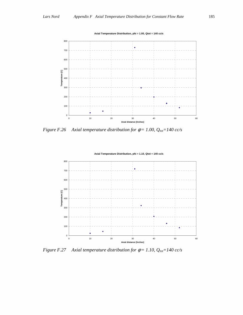
Lars Nord Appendix F Axial Temperature Distribution for Constant Flow Rate
185
Axial Temperature Distribution, phi = 1.00, Qtot = 140 cc/s
0
100
200
300
400
500
600
700
800
0 10 20 30 40 50 60Axial distance [Inches]
Tem
pera
ture
[C]
Figure F.26 Axial temperature distribution for φ = 1.00, Qtot=140 cc/s
Axial Temperature Distribution, phi = 1.10, Qtot = 140 cc/s
0
100
200
300
400
500
600
700
800
0 10 20 30 40 50 60Axial distance [Inches]
Tem
pera
ture
[C]
Figure F.27 Axial temperature distribution for φ = 1.10, Qtot=140 cc/s
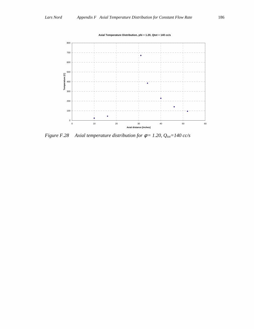
Lars Nord Appendix F Axial Temperature Distribution for Constant Flow Rate
186
Axial Temperature Distribution, phi = 1.20, Qtot = 140 cc/s
0
100
200
300
400
500
600
700
800
0 10 20 30 40 50 60Axial distance [Inches]
Tem
pera
ture
[C]
Figure F.28 Axial temperature distribution for φ = 1.20, Qtot=140 cc/s

Lars Nord Appendix F Axial Temperature Distribution for Constant Flow Rate
187
Axial Temperature Distribution, phi = 0.45, Qtot = 160 cc/s
0
100
200
300
400
500
600
700
800
0 10 20 30 40 50 60Axial distance [Inches]
Tem
pera
ture
[C]
Figure F.29 Axial temperature distribution for φ = 0.45, Qtot=160 cc/s
Axial Temperature Distribution, phi = 0.50, Qtot = 160 cc/s
0
100
200
300
400
500
600
700
800
0 10 20 30 40 50 60Axial distance [Inches]
Tem
pera
ture
[C]
Figure F.30 Axial temperature distribution for φ = 0.50, Qtot=160 cc/s

Lars Nord Appendix F Axial Temperature Distribution for Constant Flow Rate
188
Axial Temperature Distribution, phi = 0.60, Qtot = 160 cc/s
0
100
200
300
400
500
600
700
800
0 10 20 30 40 50 60Axial distance [Inches]
Tem
pera
ture
[C]
Figure F.31 Axial temperature distribution for φ = 0.60, Qtot=160 cc/s
Axial Temperature Distribution, phi = 0.70, Qtot = 160 cc/s
0
100
200
300
400
500
600
700
800
0 10 20 30 40 50 60Axial distance [Inches]
Tem
pera
ture
[C]
Figure F.32 Axial temperature distribution for φ = 0.70, Qtot=160 cc/s

Lars Nord Appendix F Axial Temperature Distribution for Constant Flow Rate
189
Axial Temperature Distribution, phi = 1.20, Qtot = 160 cc/s
0
100
200
300
400
500
600
700
800
0 10 20 30 40 50 60Axial distance [Inches]
Tem
pera
ture
[C]
Figure F.33 Axial temperature distribution for φ =1.20, Qtot=160 cc/s
Axial Temperature Distribution, phi = 1.30, Qtot = 160 cc/s
0
100
200
300
400
500
600
700
800
0 10 20 30 40 50 60Axial distance [Inches]
Tem
pera
ture
[C]
Figure F.34 Axial temperature distribution for φ =1.30, Qtot=160 cc/s
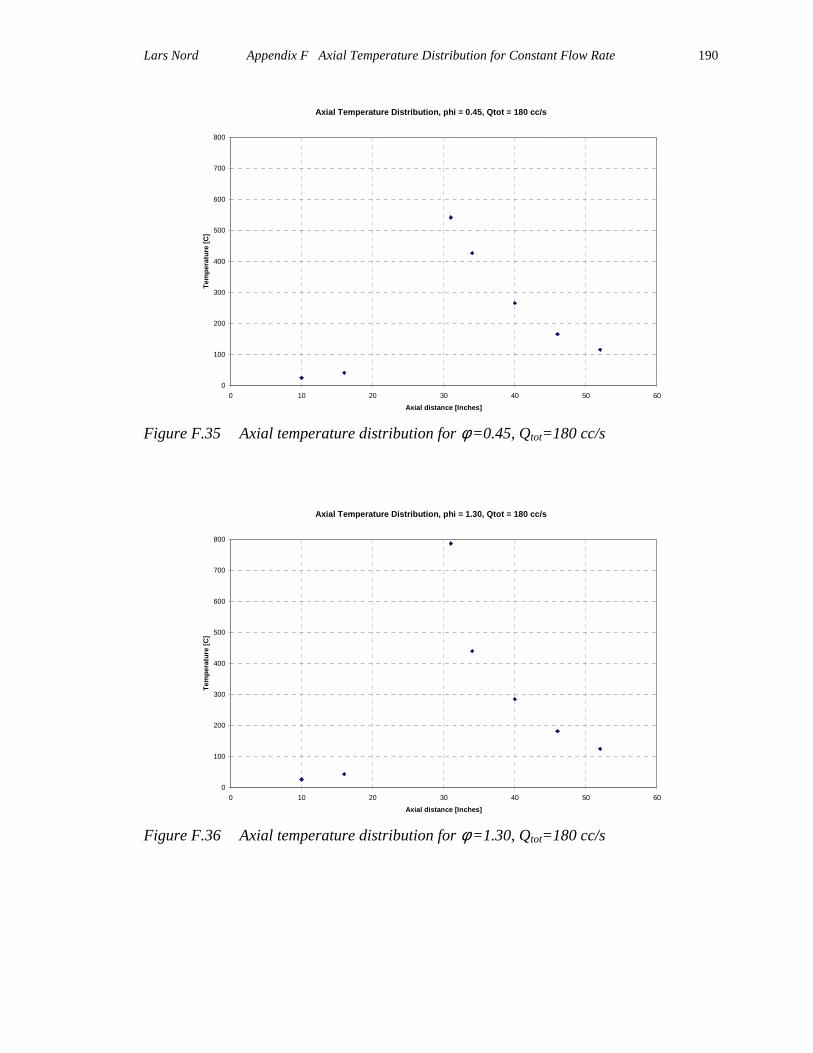
Lars Nord Appendix F Axial Temperature Distribution for Constant Flow Rate
190
Axial Temperature Distribution, phi = 0.45, Qtot = 180 cc/s
0
100
200
300
400
500
600
700
800
0 10 20 30 40 50 60Axial distance [Inches]
Tem
pera
ture
[C]
Figure F.35 Axial temperature distribution for φ =0.45, Qtot=180 cc/s
Axial Temperature Distribution, phi = 1.30, Qtot = 180 cc/s
0
100
200
300
400
500
600
700
800
0 10 20 30 40 50 60Axial distance [Inches]
Tem
pera
ture
[C]
Figure F.36 Axial temperature distribution for φ =1.30, Qtot=180 cc/s
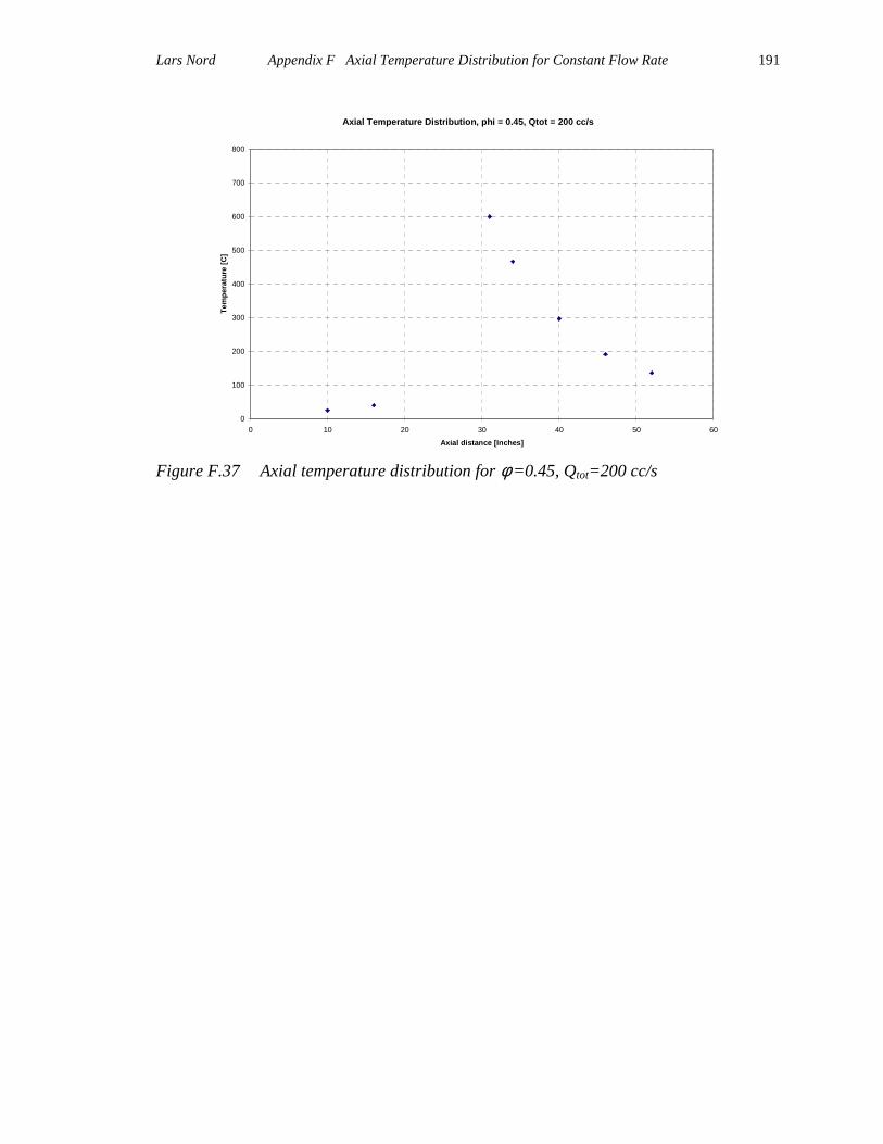
Lars Nord Appendix F Axial Temperature Distribution for Constant Flow Rate
191
Axial Temperature Distribution, phi = 0.45, Qtot = 200 cc/s
0
100
200
300
400
500
600
700
800
0 10 20 30 40 50 60Axial distance [Inches]
Tem
pera
ture
[C]
Figure F.37 Axial temperature distribution for φ =0.45, Qtot=200 cc/s

192
Vita
Lars Nord was born in October 18, 1972 and grew up in Soderhamn, Sweden. He
graduated from Polhemsskolan, Gavle, 1992, where he went to high school studying
Mechanical Engineering. A year later, he started his university studies at the department
of Mechanical Engineering at Lulea University of Technology in Sweden. After
finishing the class work in four years, he spent 5 months at ABB STAL working on a
project involving pressure pulsations in gas turbine combustion chambers to complete his
degree. After the degree he received a scholarship at the department of Mechanical
Engineering at Virginia Tech and started his graduate studies there in January of 1998.
The research at Virginia Tech was in the field of thermoacoustics; a path already started
at ABB STAL. The class work was finished in May of 1999, when he began working at
ABB Power Generation, Inc., in Richmond, VA, in the field of gas turbine performance,
emissions, and pulsations.