triggering in the horizontal rijke tube: non-normality, transient growth...
TRANSCRIPT
J. Fluid Mech. (2011), vol. 667, pp. 272–308. c© Cambridge University Press 2010
doi:10.1017/S0022112010004453
Triggering in the horizontal Rijke tube:non-normality, transient growth
and bypass transition
MATTHEW P. JUNIPER†Department of Engineering, University of Cambridge, Trumpington Street, Cambridge CB2 1PZ, UK
(Received 23 November 2009; revised 13 August 2010; accepted 17 August 2010;
first published online 25 November 2010)
With a sufficiently large impulse, a thermoacoustic system can reach self-sustainedoscillations even when it is linearly stable, a process known as triggering. In thispaper, a procedure is developed to find the lowest initial energy that can triggerself-sustained oscillations, as well as the corresponding initial state. This is known asthe ‘most dangerous’ initial state. The procedure is based on adjoint looping of thenonlinear governing equations, combined with an optimization routine. It is developedfor a simple model of a thermoacoustic system, the horizontal Rijke tube, and can beextended to more sophisticated thermoacoustic models. It is observed that the mostdangerous initial state grows transiently towards an unstable periodic solution beforegrowing to a stable periodic solution. The initial energy required to trigger these self-sustained oscillations is much lower than the energy of the oscillations themselves andslightly lower than the lowest energy on the unstable periodic solution. It is shownthat this transient growth arises due to non-normality of the governing equations. Thisis analogous to the sequence of events observed in bypass transition to turbulencein fluid mechanical systems and has the same underlying cause. The most dangerousinitial state is calculated as a function of the heat-release parameter. It is found thatself-sustained oscillations can be reached over approximately half the linearly stabledomain. Transient growth in real thermoacoustic systems is 105–106 times greaterthan that in this simple model. One practical conclusion is that, even in the linearlystable regime, it may take very little initial energy for a real thermoacoustic system totrigger to high-amplitude self-sustained oscillations through the mechanism describedin this paper.
Key words: acoustics, instability, transition to turbulence
1. IntroductionIt is well known that the laminar flow in a round pipe becomes turbulent at a
Reynolds number between 1000 and 10 000. It is also well known that this laminarflow has no unstable eigenvalues at any Reynolds number. How then can smallperturbations grow? The likely mechanism is summarized by Trefethen et al. (1993),following work by Butler & Farrell (1992) and Reddy & Henningson (1993). It hasbecome known as bypass transition to turbulence because it bypasses traditionalstability theory’s requirement for an unstable eigenvalue. The mechanism relies on
† Email address for correspondence: [email protected]
Triggering in the horizontal Rijke tube 273
the fact that the linear stability operator is non-normal. This means that certainperturbations can grow transiently even when the system is linearly stable. These thentrigger turbulence through nonlinear mechanisms. A review of this research and morerecent developments in the field can be found in Schmid (2007).
There is an analogous mechanism in thermoacoustics, through which a smallperturbation evolves to high-amplitude self-sustained oscillations even when theunperturbed system has no unstable eigenvalues. This is known as triggering. It hasbeen observed in solid rocket motors, liquid rocket motors and laboratory experiments.It is summarized in Zinn & Lieuwen (2005) (p. 19): ‘Although large-amplitudedisturbances are generally required to initiate unstable oscillations in nonlinearlyunstable systems, a system may be nonlinearly unstable at low-amplitude disturbancesthat are of the order of the background noise level. This scenario is somewhat analogousto the hydrodynamic stability of a laminar Poiseuille flow’. Although flow instabilitydiffers from thermoacoustics and turbulence differs from self-sustained oscillations,the two situations are both non-normal and nonlinear, which suggests that bypasstransition and triggering could be similar. The broad aim of this paper is to use theframework of bypass transition in fluid mechanics to provide a stronger link betweenstudies of non-normality and studies of nonlinearity in thermoacoustics, such asBalasubramanian & Sujith (2008a) and Ananthkrishnan, Deo & Culick (2005).
1.1. Bypass transition and the failure of linear analysis in hydrodynamics
The stability of a laminar flow is often investigated by calculating the eigenvalues ofsmall linear perturbations to that flow. If at least one eigenvalue is unstable, then theflow is linearly unstable. If all eigenvalues are stable, then the flow is linearly stable.The critical parameter between these two states (usually a Reynolds number) can becalculated and it might seem sensible to assume that this is the critical parameter forthe onset of turbulence.
Unfortunately, this technique often fails. For instance, Hagen–Poiseuille flow islinearly stable at all Reynolds numbers but becomes turbulent at Re ≈ 2000. PlanePoiseuille flow is linearly stable up to Re = 5772 but becomes turbulent at Re ≈ 1000.Plane Couette flow is linearly stable at all Reynolds numbers but becomes turbulentat Re ≈ 360. One notable success is Benard convection, which is linearly stable up toRe ≈ 1708 and becomes turbulent also around Re ≈ 1700.
Eigenvalue analysis fails in the first three flows because their linearized stabilityoperators are non-normal. It succeeds in the fourth flow because its linearized stabilityoperator is normal. (A matrix or operator L is normal, or self-adjoint, if it satisfiesL+L= LL+, where L+ is the adjoint of L.) Non-normal stability operators can causevery high transient growth, typically 104–106 times the initial perturbation energy,even in situations that are linearly stable (Schmid & Henningson 2001). This transientgrowth is a key component of bypass transition in the first three flows.
In flow instability, Schmid & Henningson (2001) divide bypass transition into fivestages. The first stage is initiation of small perturbations to the flow. The secondstage is linear amplification of these perturbations due to non-normal growth. Thethird stage is nonlinear saturation towards a new steady or quasi-steady periodicstate. The fourth stage is growth of secondary instabilities on top of this periodicbase flow. The fifth stage is breakdown to turbulence, where nonlinearities and/orsymmetry-breaking instabilities excite an increasing number of scales in the flow. Thisidealization provides a useful framework with which to view bypass transition, evenfor complicated flows.
274 M. P. Juniper
A flow can also be considered as a dynamical system, as in Skufca, Yorke &Eckhardt (2006) for parallel shear flow and Schneider, Eckhardt & Yorke (2007) andDuguet, Willis & Kerswell (2008) for pipe flow. A boundary in state space is identifiedbetween trajectories that decay to a laminar solution and trajectories that evolve toa turbulent solution. Trajectories that are attracted to this boundary from lowerenergy states exhibit the transient growth identified in stage 2. Having identified thisboundary, which Skufca et al. (2006) call the ‘edge of chaos’, stage 4 can be describedin more detail. This boundary contains several heteroclinic saddle points and atleast one local relative attractor, each corresponding to a periodic travelling-wavesolution (Duguet, Willis & Kerswell 2008). The state wanders from the vicinity of onetravelling-wave solution to the vicinity of another and so on until it reaches a localrelative attractor, where it either evolves towards the laminar solution or towardsa turbulent solution. Its final state very sensitively depends on its initial state. Thetravelling-wave solutions correspond to the quasi-steady periodic state identified instage 3 of Schmid & Henningson (2001).
1.2. Triggering and the need for nonlinearity and non-normality in thermoacoustics
In this paper, a similar conceptual framework is applied to thermoacoustic triggering,which also involves non-normality and nonlinearity. The role of nonlinearity issummarized by Ananthkrishnan et al. (2005), who show that the system must haveeither a subcritical bifurcation or a supercritical bifurcation followed by a foldbifurcation in order to trigger. This is similar to the requirements for bypass transition(Henningson & Reddy 1994). In such a system, there are two (or more) stable solutionsto the governing equations. The first is a stable fixed point at zero amplitude and thesecond is a stable periodic solution at finite amplitude. When the system is at thestable fixed point, a sufficiently large impulse can knock it into the basin of attractionof the self-sustained oscillation. This is triggering. Such systems are sometimes called‘linearly stable but nonlinearly unstable’ (Zinn & Lieuwen 2005), but it should bestressed that, from a dynamical systems’ point of view, both solutions are stable.
Noiray et al. (2008) present a practical and novel method to predict whether asystem will be susceptible to triggering. They measure the flame’s OH∗ emission as afunction of forcing frequency and amplitude, from which they interpolate to obtaina flame describing function (FDF). Then they enter this into a frequency-domainnonlinear stability analysis to predict the self-excited behaviour of the system. Theyvalidate this against the experimentally observed self-excited behaviour and therebyaccount for the nonlinear aspects of triggering, mode switching and hysteresis. Ina system that is susceptible to triggering, an unstable periodic solution sits on theboundary between the basins of attraction of the stable fixed point and the stableperiodic solution (§ 3.2). This is the steady or quasi-steady periodic state described instage 3 of § 1.1. The results in figure 9 of Noiray et al. (2008) show that the systemtriggers when its amplitude infinitesimally exceeds that of this unstable periodicsolution, corresponding to stage 4 of § 1.1. Their study, however, freezes harmonicsto the fundamental mode. It will be shown in § 3.4 that this precludes non-normaltransient growth, which means that their method cannot account for the growthtowards the periodic state described in stage 2 of § 1.1. To account for this growth,non-normality must also be considered.
The role of non-normality in thermoacoustics was first considered byBalasubramanian & Sujith (2008a) for the Rijke tube, by Balasubramanian &Sujith (2008b) for a Burke–Schumann flame in a tube and by Nagaraja, Kedia &Sujith (2009) for a generic n–τ combustion model. These papers show that the
Triggering in the horizontal Rijke tube 275
linearized governing equations are non-normal, which means that their correspondingeigenvectors are non-orthogonal. This is a general feature of eigenvectors inthermoacoustics (Nicoud et al. 2007), and means that some initial states arecomposed of eigenfunctions with large amplitudes that largely cancel out. If theeigenfunctions of such states decay at different rates, the states grow initiallyeven if all the eigenfunctions eventually decay (Schmid 2007). Using linear algebra,Balasubramanian & Sujith (2008a) found the states that have maximum transientgrowth away from the stable fixed point and, using nonlinear time marching, showedthat these states can grow to self-sustained oscillations in a linearly stable system.This paper examines this process in more detail and, in particular, examines the statesthat cause maximum transient growth towards the unstable periodic solution.
1.3. The structure of this paper
This paper examines the simple model of thermoacoustic oscillations in the horizontalRijke tube studied by Balasubramanian & Sujith (2008a). Although this model ismuch less complex than real thermoacoustic systems, it contains important elementsof real systems, such as a time delay between velocity and heat-release perturbationsas well as a heat-release rate that depends nonlinearly on the velocity. Usually, thenonlinear governing equations are used but, occasionally, the linear equations arerequired. The model and the linearizations are described in § 2.1, together with thethree thermoacoustic systems that are used as examples.
A classical nonlinear analysis is performed in § 3. The systems’ bifurcation diagramsare plotted as a function of the heat-release parameter. A continuation method isused to find the periodic solutions, whose stability is determined from their Floquetmultipliers. Careful consideration of the basins of attraction of the periodic solutionsreveals the role that the unstable periodic solution plays in the triggering process.
Previous studies have considered linear transient growth around the stable fixedpoint. In § 3.3, linear transient growth is considered around the unstable periodicsolution, which is more relevant to triggering. A linear analysis is limited to thevicinity of the unstable periodic solution; so, in § 4, a procedure is developed to findoptimal initial states of the nonlinear governing equations. This is used to find theinitial states that trigger to self-sustained oscillations from the lowest possible energy,which are called the ‘most dangerous’ initial states.
Having found these states, the linear evolution and nonlinear evolution arecompared in § 5 in order to determine whether the transient growth is caused bynon-normality, nonlinearity, or some combination of the two. The triggering processis then compared with that of bypass transition within the framework introduced in§ 1.1 and found to be similar but simpler.
In § 6, the procedure is applied over the full range of the heat-release parameter atwhich the system is susceptible to triggering. This gives the bound, in terms of theinitial perturbation energy, below which the system can never trigger to self-sustainedoscillations, which is called the ‘safe operating region’. In more complex systems, thisbound will have important engineering significance.
It turns out that the thermoacoustic system in this paper has two stable periodicsolutions. In §§ 3–6, the concepts are described with reference to the first solution. In§ 7, the second solution is introduced.
This paper describes an idealized situation, in which triggering occurs from awell-defined initial state in a noiseless system. It could be difficult to create such asystem in the laboratory; so the implications for experiments, in particular the effectof different types of noise, are discussed in § 8.
276 M. P. Juniper
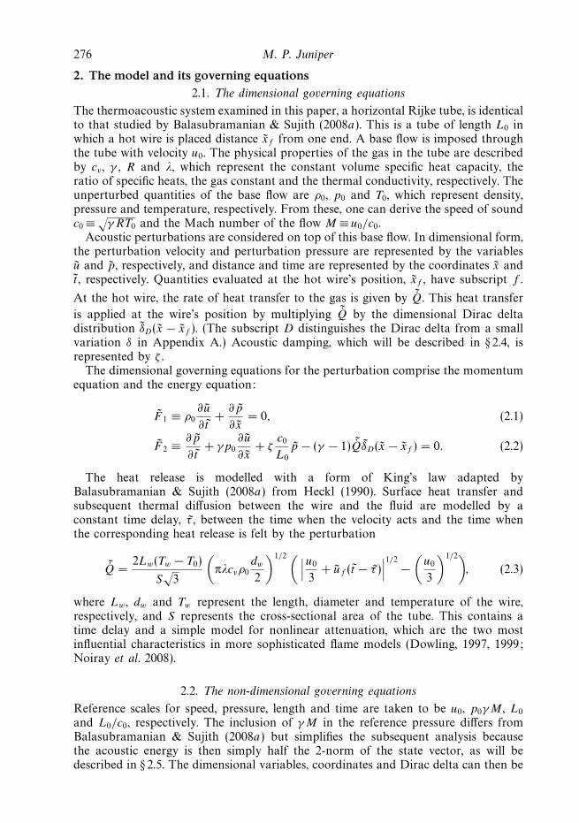
2. The model and its governing equations2.1. The dimensional governing equations
The thermoacoustic system examined in this paper, a horizontal Rijke tube, is identicalto that studied by Balasubramanian & Sujith (2008a). This is a tube of length L0 inwhich a hot wire is placed distance xf from one end. A base flow is imposed throughthe tube with velocity u0. The physical properties of the gas in the tube are describedby cv , γ , R and λ, which represent the constant volume specific heat capacity, theratio of specific heats, the gas constant and the thermal conductivity, respectively. Theunperturbed quantities of the base flow are ρ0, p0 and T0, which represent density,pressure and temperature, respectively. From these, one can derive the speed of soundc0 ≡
√γRT0 and the Mach number of the flow M ≡ u0/c0.
Acoustic perturbations are considered on top of this base flow. In dimensional form,the perturbation velocity and perturbation pressure are represented by the variablesu and p, respectively, and distance and time are represented by the coordinates x andt , respectively. Quantities evaluated at the hot wire’s position, xf , have subscript f .
At the hot wire, the rate of heat transfer to the gas is given by ˜Q. This heat transfer
is applied at the wire’s position by multiplying ˜Q by the dimensional Dirac deltadistribution δD(x − xf ). (The subscript D distinguishes the Dirac delta from a smallvariation δ in Appendix A.) Acoustic damping, which will be described in § 2.4, isrepresented by ζ .
The dimensional governing equations for the perturbation comprise the momentumequation and the energy equation:
F 1 ≡ ρ0
∂u
∂t+
∂p
∂x= 0, (2.1)
F 2 ≡ ∂p
∂t+ γp0
∂u
∂x+ ζ
c0
L0
p − (γ − 1) ˜QδD(x − xf ) = 0. (2.2)
The heat release is modelled with a form of King’s law adapted byBalasubramanian & Sujith (2008a) from Heckl (1990). Surface heat transfer andsubsequent thermal diffusion between the wire and the fluid are modelled by aconstant time delay, τ , between the time when the velocity acts and the time whenthe corresponding heat release is felt by the perturbation
˜Q =2Lw(Tw − T0)
S√
3
(πλcvρ0
dw
2
)1/2 ( ∣∣∣u0
3+ uf (t − τ )
∣∣∣1/2 −(
u0
3
)1/2), (2.3)
where Lw , dw and Tw represent the length, diameter and temperature of the wire,respectively, and S represents the cross-sectional area of the tube. This contains atime delay and a simple model for nonlinear attenuation, which are the two mostinfluential characteristics in more sophisticated flame models (Dowling, 1997, 1999;Noiray et al. 2008).
2.2. The non-dimensional governing equations
Reference scales for speed, pressure, length and time are taken to be u0, p0γM , L0
and L0/c0, respectively. The inclusion of γM in the reference pressure differs fromBalasubramanian & Sujith (2008a) but simplifies the subsequent analysis becausethe acoustic energy is then simply half the 2-norm of the state vector, as will bedescribed in § 2.5. The dimensional variables, coordinates and Dirac delta can then be
Triggering in the horizontal Rijke tube 277
written as
u = u0u, p = p0γMp, x = L0x, t = (L0/c0)t, ˜δD(x−xf ) = δD(x−xf )/L0, (2.4)
where the quantities without a tilde or subscript 0 are dimensionless.Substituting (2.4) into the dimensional governing equations (2.1) and (2.2) and
making use of the definition of c0 and the ideal gas law, p0 = ρ0RT0, gives thedimensionless governing equations
F1 ≡ ∂u
∂t+
∂p
∂x= 0, (2.5)
F2 ≡ ∂p
∂t+
∂u
∂x+ ζp − β
( ∣∣∣∣13 + uf (t − τ )
∣∣∣∣1/2
−(
1
3
)1/2 )δD(x − xf ) = 0, (2.6)
where
β ≡ 1
p0√
u0
(γ − 1)
γ
2Lw(Tw − T0)
S√
3
(πλcvρ0
dw
2
)1/2
. (2.7)
The system has four control parameters: ζ , which is the damping; β , whichencapsulates all relevant information about the hot wire, base velocity and ambientconditions; τ , which is the time delay; and xf , which is the position of the wire.The heat-release parameter, β , is equivalent to k/γM in Balasubramanian & Sujith(2008a).
2.3. The boundary conditions and the discretized governing equations
When appropriate boundary conditions in x are set, the governing equations (2.5) and(2.6) reduce to an initial value problem in t . For the system examined in this paper,∂u/∂x and p are both set to zero at the ends of the tube. These boundary conditionsare enforced by choosing basis sets that match these boundary conditions:
u(x, t) =
N∑j=1
ηj (t) cos(jπx), (2.8)
p(x, t) = −N∑
j=1
(ηj (t)
jπ
)sin(jπx), (2.9)
where the relationship between ηj and ηj has not yet been specified. In thisdiscretization, which is sometimes known as a Galerkin discretization, all the basisvectors are orthogonal.
The state of the system is given by the amplitudes of the Galerkin modes thatrepresent velocity, ηj , and those that represent pressure, ηj /jπ. These are giventhe notation u ≡ (η1, . . . , ηN )T and p ≡ (η1/π, . . . , ηN/Nπ)T . The state vector of thediscretized system is the column vector x ≡ (u; p).
The governing equations are discretized by substituting (2.8) and (2.9) into (2.5)and (2.6). As described in § 2.4, the damping, ζ , is dealt with by assigning a dampingparameter, ζj , to each mode. Equation (2.6) is then multiplied by sin(kπx) andintegrated over the domain x = [0, 1]. The governing equations then reduce to twodelay differential equations (DDEs) for each mode, j :
F1G ≡ d
dtηj − jπ
(ηj
jπ
)= 0, (2.10)
278 M. P. Juniper
F2G ≡ d
dt
(ηj
jπ
)+ jπηj + ζj
(ηj
jπ
)· · ·
+ 2β
( ∣∣∣∣13 + uf (t − τ )
∣∣∣∣1/2
−(
1
3
)1/2 )sin(jπxf ) = 0, (2.11)
where
uf (t − τ ) =
N∑k=1
ηk(t − τ ) cos(kπxf ). (2.12)
2.4. Damping
For the system examined in this paper, p and ∂u/∂x are both set to zero at theends of the tube, which means that the system cannot dissipate acoustic energy bydoing work on the surroundings. Furthermore, the acoustic waves are planar, whichmeans that the system cannot dissipate acoustic energy in the viscous and thermalboundary layers at the tube walls. Both types of dissipation are modelled by thedamping parameter for each mode:
ζj = c1j2 + c2j
1/2, (2.13)
where c1 and c2 are the same for each mode. This model was used inBalasubramanian & Sujith (2008a) and Nagaraja et al. (2009) and was based oncorrelations developed by Matveev (2003) from models in Landau & Lifshitz (1959).
2.5. The definition of the acoustic energy norm
For the optimization procedure, it is necessary to define some measure of the sizeof the perturbations. Several measures are possible and each could give a differentoptimal. The most convenient measure is the acoustic energy per unit volume, E,because it is easy to calculate and has a simple physical interpretation (Nagarajaet al. 2009).
The acoustic energy per unit volume, E, consists of a kinetic component, Ek , anda pressure potential component, Ep . In dimensional form, it is given by
E = Ek + Ep =1
2ρ0
(u2 +
p2
ρ20c
20
). (2.14)
Substituting for u and p from (2.4), making use of the ideal gas relation anddefining the reference scale for energy per unit volume to be ρ0u
20, the dimensionless
acoustic energy per unit volume, E, is given by
E =1
2u2 +
1
2p2 =
1
2
N∑j=1
η2j +
1
2
N∑j=1
(ηj
jπ
)2
=1
2xH x =
1
2‖x‖2, (2.15)
where ‖ · ‖ represents the 2-norm. The rate of change of the acoustic energy with timeis
dE
dt= u
du
dt+ p
dp
dt=
N∑j=1
ηj
dηj
dt+
N∑j=1
(ηj
jπ
)d
dt
(ηj
jπ
)= −
N∑j=1
ζj
(ηj
jπ
)2
−N∑
j=1
2β
(ηj
jπ
)( ∣∣∣∣13 + uf (t − τ )
∣∣∣∣1/2
−(
1
3
)1/2 )sin(jπxf ). (2.16)
Triggering in the horizontal Rijke tube 279
The first term on the right-hand side of (2.16) represents damping and is alwaysnegative. The second term is the instantaneous value of pQ and is the rate at whichthermal energy is transferred to acoustic energy at the wire. It is worth noting thatthis transfer of energy can be in either direction.
2.6. The linearized governing equations
Non-normality, which is central to this paper, is a linear phenomenon. It is most easilyexamined when the governing equations are linearized around x =0 and expressed inthe form dx/dt = Lx, where x represents the state of the system and L represents theevolution operator or matrix. Two linearizations are required to express the governingequations in this form. The first linearization, which is valid for uf (t − τ ) � 1/3, isperformed on the square-root term in (2.6) and (2.11):( ∣∣∣∣13 + uf (t − τ )
∣∣∣∣1/2
−(
1
3
)1/2 )≈
√3
2uf (t − τ ). (2.17)
This produces a system of linear DDEs: dx/dt = L1x(t) + L2x(t − τ ), where L1 is anormal matrix and L2 is a non-normal matrix. It is possible to find the eigenvaluesof this linear DDE system (Selimefendigila, Sujith & Polifke 2010) and to quantifythe non-normality of L2 but, in Balasubramanian & Sujith (2008a) and this paper, asecond linearization is performed on the time delay:
uf (t − τ ) ≈ uf (t) − τ∂uf (t)
∂t
=
N∑k=1
ηk(t) cos(kπxf ) − τ
N∑k=1
kπ
(ηk(t)
kπ
)cos(kπxf ). (2.18)
This linearization is valid only for the Galerkin modes for which τ � Tj , whereTj = 2/j is the period of the j th Galerkin mode. Equations (2.17) and (2.18) aresubstituted into (2.11) to give the linearized governing equations
F1G ≡ d
dtηj − jπ
(ηj
jπ
)= 0, (2.19)
F2G ≡ d
dt
(ηj
jπ
)+ jπηj + ζj
(ηj
jπ
)· · ·
+√
3βsj
N∑k=1
ηkck −√
3βτsj
N∑k=1
kπ
(ηk
kπ
)ck = 0, (2.20)
where sj ≡ sin(jπxf ) and ck ≡ cos(kπxf ). This is a set of linear ordinary differentialequations (ODEs), which can be expressed in the matrix form
d
dtx =
d
dt
(up
)=
(LT L LT R
LBL LBR
)(up
)= Lx. (2.21)
The rate of change of energy dE/dt can be found either by substituting (2.17) and(2.18) into (2.16) or by evaluating xT Lx. This gives
dE
dt= −
N∑j=1
ζj
(ηj
jπ
)2
−√
3β
N∑j=1
N∑k=1
sj ck
(ηj
jπ
)ηk +
√3βτ
N∑j=1
N∑k=1
sj ckkπ
(ηj
jπ
)(ηk
kπ
).
(2.22)
280 M. P. Juniper
2.7. The systems examined in this paper
The thermoacoustic system examined in this paper has xf = 0.3, c1 = 0.05, c2 = 0.01and τ = 0.02. These values are typical of a laboratory Rijke tube. (τ is slightly lowerthan that found in Heckl (1990), who used τ = 0.05.) For the nonlinear results, theDDEs (see (2.10)–(2.11)) are integrated from t = 0. This requires information aboutuf for t ∈ [−τ, 0) and adds as many degrees of freedom as there are time steps inthis time period. In this paper, uf is set to zero in this period in order to freeze thesedegrees of freedom. Although this is artificial, the effect is small because the timedelay, τ =0.02, is very much smaller than the period over which transient growthtakes place, which is of order 2–20.
One advantage of the Galerkin discretization is that concepts can be demonstratedon a small dimensional system and then readily extended to a large dimensionalsystem. In this paper, the system is considered with 1, 3 and 10 Galerkin modes,labelled systems A, B and C, respectively. System A has two degrees of freedomand exhibits nonlinear characteristics but no non-normal transient growth over onecycle around the unstable periodic solution. System B has six degrees of freedomand exhibits both nonlinear and non-normal characteristics. System C is qualitativelyidentical to system B but has 20 degrees of freedom and is more representative of anactual thermoacoustic system.
For direct time marching, (2.10)–(2.11) are integrated with a fourth-order Runge–Kutta algorithm with δt = 0.005. For adjoint looping, the gradient information isfound by integrating the equations in § B.6 with a first-order Euler algorithm withδt = 0.00005. These time steps are sufficiently small that the results are not sensitiveto the time step.
3. The lower periodic solutions of the nonlinear governing equationsIn § 7 it will be shown that there are two stable periodic solutions to the governing
equations. The lower solution has velocity perturbations with amplitude less thanthe mean flow. The higher solution has velocity perturbations with amplitude greaterthan the mean flow. For simplicity, §§ 3–6 will consider only the lower solution, as ifthe higher solution did not exist. The higher solution will be introduced in § 7.
3.1. The fixed point and periodic solutions on a bifurcation diagram
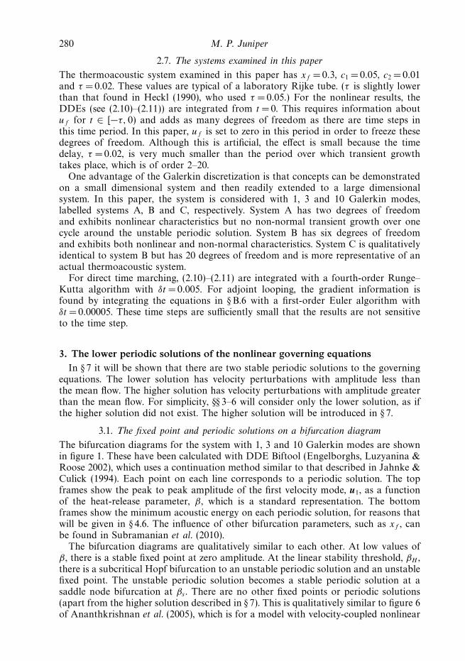
The bifurcation diagrams for the system with 1, 3 and 10 Galerkin modes are shownin figure 1. These have been calculated with DDE Biftool (Engelborghs, Luzyanina &Roose 2002), which uses a continuation method similar to that described in Jahnke &Culick (1994). Each point on each line corresponds to a periodic solution. The topframes show the peak to peak amplitude of the first velocity mode, u1, as a functionof the heat-release parameter, β , which is a standard representation. The bottomframes show the minimum acoustic energy on each periodic solution, for reasons thatwill be given in § 4.6. The influence of other bifurcation parameters, such as xf , canbe found in Subramanian et al. (2010).
The bifurcation diagrams are qualitatively similar to each other. At low values ofβ , there is a stable fixed point at zero amplitude. At the linear stability threshold, βH ,there is a subcritical Hopf bifurcation to an unstable periodic solution and an unstablefixed point. The unstable periodic solution becomes a stable periodic solution at asaddle node bifurcation at βs . There are no other fixed points or periodic solutions(apart from the higher solution described in § 7). This is qualitatively similar to figure 6of Ananthkrishnan et al. (2005), which is for a model with velocity-coupled nonlinear
Triggering in the horizontal Rijke tube 281
0.8 0.9 1.0 1.1 1.2
0.8 0.9 1.0 1.1 1.2
0
0.5
1.0
1.5
max
(u1)
– m
in(u
1)(a) N = 1
βH
0
0.05
0.10
0.15
0.20
0.25
Heat release parameter, β
Em
in
(d)
0.6 0.7 0.8 0.9 1.0 0.6 0.7 0.8 0.9 1.0
0.6 0.7 0.8 0.9 1.0 0.6 0.7 0.8 0.9 1.0
0
0.5
1.0
1.5
(b) N = 3
0
0.05
0.10
0.15
0.20
0.25
Heat release parameter, β
(e)
0
0.5
1.0
1.5
(c) N = 10
0
0.05
0.10
0.15
0.20
0.25
Heat release parameter, β
( f )
β =
1.1
0
β =
0.7
5
β =
0.7
5
βH
β =
1.1
0
β =
0.7
5
βsβs
βH
β =
0.7
5
βs
Figure 1. Bifurcation diagrams as a function of heat-release parameter, β , for the 1, 3 and10 Galerkin mode systems (left to right). The top frames show the peak to peak amplitudeof the first velocity mode. The bottom frames show the minimum acoustic energy on theperiodic solutions. The solution with zero amplitude is stable up to β = βH , where there is aHopf bifurcation to an unstable periodic solution (dashed line). The unstable periodic solutionbecomes a stable periodic solution (solid line) at a saddle node bifurcation, βs .
−1.0 −0.5 0 0.5 1.0
−1.0
−0.5
0
0.5
1.0
System A
Real (µ)−1.0 −0.5 0 0.5 1.0
−1.0
−0.5
0
0.5
1.0
System B
Real (µ)−1.0 −0.5 0 0.5 1.0
−1.0
−0.5
0
0.5
1.0
System C
Real (µ)
Imag
(µ
)
UnstableNeutral
UnstableNeutralStable
UnstableNeutralStable
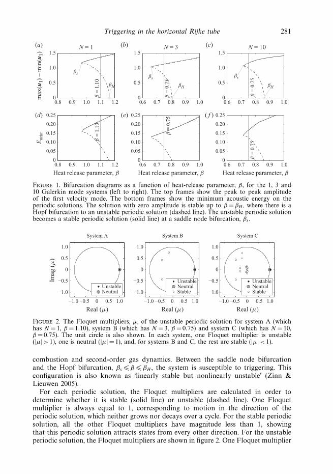
Figure 2. The Floquet multipliers, µ, of the unstable periodic solution for system A (whichhas N =1, β =1.10), system B (which has N = 3, β = 0.75) and system C (which has N = 10,β = 0.75). The unit circle is also shown. In each system, one Floquet multiplier is unstable(|µ| > 1), one is neutral (|µ| = 1), and, for systems B and C, the rest are stable (|µ| < 1).
combustion and second-order gas dynamics. Between the saddle node bifurcationand the Hopf bifurcation, βs � β � βH , the system is susceptible to triggering. Thisconfiguration is also known as ‘linearly stable but nonlinearly unstable’ (Zinn &Lieuwen 2005).
For each periodic solution, the Floquet multipliers are calculated in order todetermine whether it is stable (solid line) or unstable (dashed line). One Floquetmultiplier is always equal to 1, corresponding to motion in the direction of theperiodic solution, which neither grows nor decays over a cycle. For the stable periodicsolution, all the other Floquet multipliers have magnitude less than 1, showingthat this periodic solution attracts states from every other direction. For the unstableperiodic solution, the Floquet multipliers are shown in figure 2. One Floquet multiplier
282 M. P. Juniper
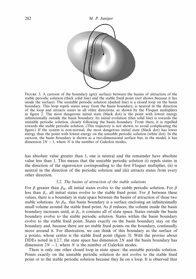
Figure 3. A cartoon of the boundary (grey surface) between the basins of attraction of thestable periodic solution (thick solid line) and the stable fixed point (not shown because it liesinside the surface). The unstable periodic solution (dashed line) is a closed loop on the basinboundary. This loop repels states away from the basin boundary, is neutral in the directionof the loop and attracts states in all other directions, as shown by the Floquet multipliersin figure 2. The most dangerous initial state (black dot) is the point with lowest energyinfinitesimally outside the basin boundary. Its initial evolution (thin solid line) is towards theunstable periodic solution, closely following the basin boundary. From there, it is repelledtowards the stable periodic solution. (This trajectory is not shown, to avoid complicating thefigure.) If the system is non-normal, the most dangerous initial state (black dot) has lowerenergy than the point with lowest energy on the unstable periodic solution (white dot). In thecartoon, the basin boundary is shown as a two-dimensional surface but, in the model, it hasdimension 2N − 1, where N is the number of Galerkin modes.
has absolute value greater than 1, one is neutral and the remainder have absolutevalue less than 1. This means that the unstable periodic solution (i) repels states inthe direction of the eigenvector corresponding to the first Floquet multiplier, (ii) isneutral in the direction of the periodic solution and (iii) attracts states from everyother direction.
3.2. The basins of attraction of the stable solutions
For β greater than βH , all initial states evolve to the stable periodic solution. For β
less than βs , all initial states evolve to the stable fixed point. For β between thesevalues, there is a boundary in state space between the basins of attraction of these twostable solutions. At βH , this basin boundary is a surface enclosing an infinitesimallysmall volume around the stable fixed point. As β reduces, the volume inside the basinboundary increases until, at βs , it contains all of state space. States outside the basinboundary evolve to the stable periodic solution. States within the basin boundaryevolve to the stable fixed point. States exactly on the basin boundary stay on theboundary and, because there are no stable fixed points on the boundary, continuallymove around it. For illustration, we can think of this boundary as the surface ofa potato, whose centre is the stable fixed point (figure 3). With the proviso aboutDDEs noted in § 2.7, the state space has dimension 2N and the basin boundary hasdimension 2N − 1, where N is the number of Galerkin modes.
There is only one other closed loop in state space: the unstable periodic solution.Points exactly on the unstable periodic solution do not evolve to the stable fixedpoint or to the stable periodic solution because they lie on a loop. It is observed that

Triggering in the horizontal Rijke tube 283
1 2 3 4 5 6 7 8 9 100
1
2
3
4(×10−3)
E
Galerkin mode
0.07
948
System A
1 2 3 4 5 6 7 8 9 100
1
2
3
4(×10−3)
Galerkin mode
System B
1 2 3 4 5 6 7 8 9 100
1
2
3
4(×10−3)
Galerkin mode
System C
0.07
121
0.11
99
Figure 4. The distribution of energy in the Galerkin modes at the lowest energy point onthe unstable periodic solution. The energy in the first mode, which greatly exceeds that in theother modes, is written on the first bar. The absolute values are significant because this isderived from a nonlinear analysis. The exact distribution of u, p and E is in table 1.
neighbouring points evolve either to the stable periodic solution or to the stable fixedpoint. There are no other stable solutions in this region of state space. Therefore, theunstable periodic solution lies on the basin boundary. We can imagine the unstableperiodic solution as a loop drawn on the surface of the potato (figure 3). This looprepels states away from the boundary, either towards the stable fixed point or towardsthe stable periodic solution, is neutral in the direction tangential to the loop, andattracts states in all other directions. Because there are no other periodic solutions orfixed points on the basin boundary, all points that start exactly on the basin boundaryand near to the unstable periodic solution must be attracted towards the unstableperiodic solution. This solution is known as an unstable attractor (Ashwin & Timme2005), or a local relative attractor. We can think of these trajectories as lines drawnon the surface of the potato, spiralling towards the loop, without ever quite reachingit (figure 3).
Returning to the framework introduced in § 1.1, this basin boundary corresponds tothe boundary that Skufca et al. (2006) call the ‘edge of chaos’ in fluid mechanics. Theunstable periodic solution, which sits on the basin boundary, corresponds to the localrelative attractor in Duguet et al. (2008) or, equivalently, the steady or quasi-steadyperiodic state identified in stage 3 of Schmid & Henningson (2001).
3.3. Transient growth around the unstable periodic solutions of systems B and C
One aim of this paper is to find the lowest energy initial state that just evolves to thestable periodic solution. This is equivalent to finding the lowest energy state on thebasin boundary. The lowest energy state on the unstable periodic solution (figure 4and table 1) is an obvious starting point because every state that starts exactly onthe basin boundary evolves towards this periodic solution and must pass nearby.The question is now whether states can evolve towards the unstable periodic solutionfrom lower energies than this state. In other words, what is the shape of the basinboundary around the unstable periodic solution? Is it convex or knobbly and doesthe lowest energy state on this loop lie at the bottom of a valley or on a slope?
To answer this, we will consider transient growth around the unstable periodicsolution. Beforehand, it is worth reviewing studies that have looked at transientgrowth around the stable fixed point, such as Balasubramanian & Sujith (2008a).To do this, the governing equations are linearized around the fixed point (§ 2.6), andthe linear stability operator, L, is calculated (2.21). The eigenvalues of L describethe long time behaviour around the fixed point but, if the operator is non-normal,
284 M. P. Juniper
Galerkin mode number
1 2 3 4 5 6 7 8 9 10 Total
A u −0.3986A p 0.0014A E 0.0794 0.0794
B u −0.3773 0.0615 0.0166B p −0.0036 0.0034 0.0010B E 0.0712 0.0018 0.0001 0.0732
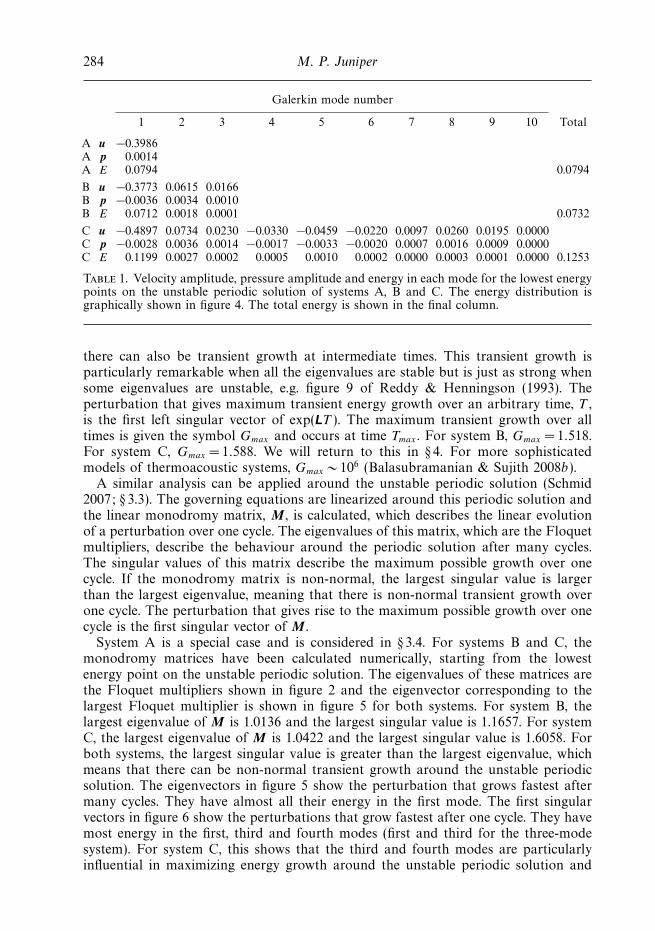
C u −0.4897 0.0734 0.0230 −0.0330 −0.0459 −0.0220 0.0097 0.0260 0.0195 0.0000C p −0.0028 0.0036 0.0014 −0.0017 −0.0033 −0.0020 0.0007 0.0016 0.0009 0.0000C E 0.1199 0.0027 0.0002 0.0005 0.0010 0.0002 0.0000 0.0003 0.0001 0.0000 0.1253
Table 1. Velocity amplitude, pressure amplitude and energy in each mode for the lowest energypoints on the unstable periodic solution of systems A, B and C. The energy distribution isgraphically shown in figure 4. The total energy is shown in the final column.
there can also be transient growth at intermediate times. This transient growth isparticularly remarkable when all the eigenvalues are stable but is just as strong whensome eigenvalues are unstable, e.g. figure 9 of Reddy & Henningson (1993). Theperturbation that gives maximum transient energy growth over an arbitrary time, T ,is the first left singular vector of exp(LT ). The maximum transient growth over alltimes is given the symbol Gmax and occurs at time Tmax . For system B, Gmax =1.518.For system C, Gmax = 1.588. We will return to this in § 4. For more sophisticatedmodels of thermoacoustic systems, Gmax ∼ 106 (Balasubramanian & Sujith 2008b).
A similar analysis can be applied around the unstable periodic solution (Schmid2007; § 3.3). The governing equations are linearized around this periodic solution andthe linear monodromy matrix, M , is calculated, which describes the linear evolutionof a perturbation over one cycle. The eigenvalues of this matrix, which are the Floquetmultipliers, describe the behaviour around the periodic solution after many cycles.The singular values of this matrix describe the maximum possible growth over onecycle. If the monodromy matrix is non-normal, the largest singular value is largerthan the largest eigenvalue, meaning that there is non-normal transient growth overone cycle. The perturbation that gives rise to the maximum possible growth over onecycle is the first singular vector of M .
System A is a special case and is considered in § 3.4. For systems B and C, themonodromy matrices have been calculated numerically, starting from the lowestenergy point on the unstable periodic solution. The eigenvalues of these matrices arethe Floquet multipliers shown in figure 2 and the eigenvector corresponding to thelargest Floquet multiplier is shown in figure 5 for both systems. For system B, thelargest eigenvalue of M is 1.0136 and the largest singular value is 1.1657. For systemC, the largest eigenvalue of M is 1.0422 and the largest singular value is 1.6058. Forboth systems, the largest singular value is greater than the largest eigenvalue, whichmeans that there can be non-normal transient growth around the unstable periodicsolution. The eigenvectors in figure 5 show the perturbation that grows fastest aftermany cycles. They have almost all their energy in the first mode. The first singularvectors in figure 6 show the perturbations that grow fastest after one cycle. They havemost energy in the first, third and fourth modes (first and third for the three-modesystem). For system C, this shows that the third and fourth modes are particularlyinfluential in maximizing energy growth around the unstable periodic solution and
Triggering in the horizontal Rijke tube 285
1 2 3 4 5 6 7 8 9 100
0.05
0.10
0.15
E E0
Galerkin mode
0.49
87
System B
1 2 3 4 5 6 7 8 9 100
0.05
0.10
0.15
Galerkin mode
System C
0.49
26
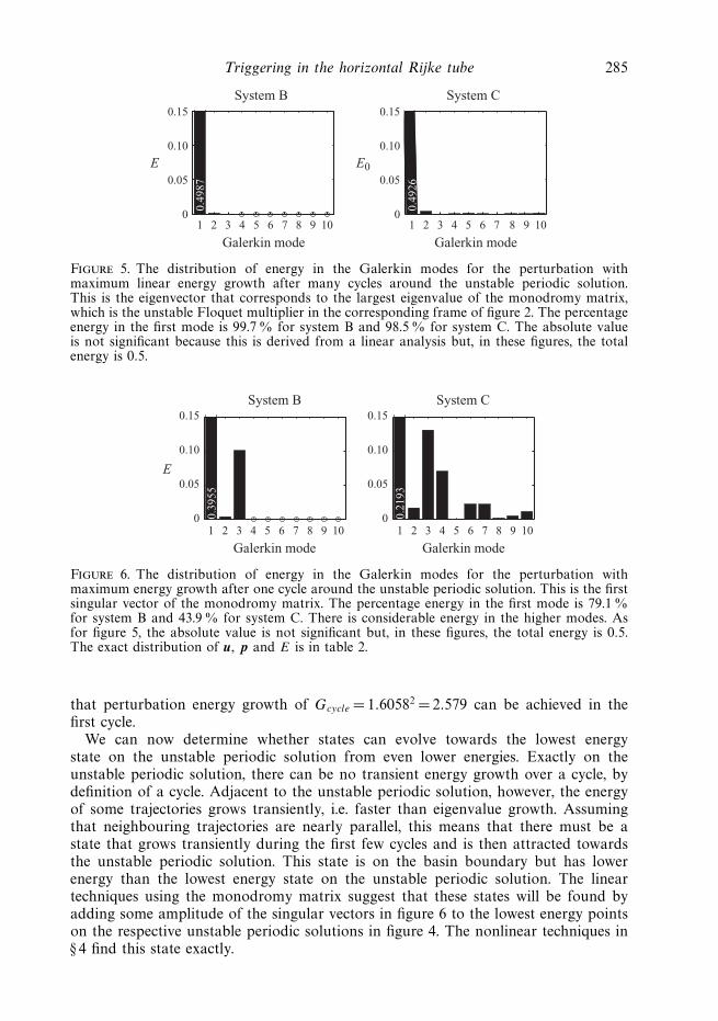
Figure 5. The distribution of energy in the Galerkin modes for the perturbation withmaximum linear energy growth after many cycles around the unstable periodic solution.This is the eigenvector that corresponds to the largest eigenvalue of the monodromy matrix,which is the unstable Floquet multiplier in the corresponding frame of figure 2. The percentageenergy in the first mode is 99.7 % for system B and 98.5 % for system C. The absolute valueis not significant because this is derived from a linear analysis but, in these figures, the totalenergy is 0.5.
1 2 3 4 5 6 7 8 9 100
0.05
0.10
0.15
E
Galerkin mode1 2 3 4 5 6 7 8 9 10
Galerkin mode
0.39
55
System B
0
0.05
0.10
0.15System C
0.21
93
Figure 6. The distribution of energy in the Galerkin modes for the perturbation withmaximum energy growth after one cycle around the unstable periodic solution. This is the firstsingular vector of the monodromy matrix. The percentage energy in the first mode is 79.1 %for system B and 43.9% for system C. There is considerable energy in the higher modes. Asfor figure 5, the absolute value is not significant but, in these figures, the total energy is 0.5.The exact distribution of u, p and E is in table 2.
that perturbation energy growth of Gcycle = 1.60582 = 2.579 can be achieved in thefirst cycle.
We can now determine whether states can evolve towards the lowest energystate on the unstable periodic solution from even lower energies. Exactly on theunstable periodic solution, there can be no transient energy growth over a cycle, bydefinition of a cycle. Adjacent to the unstable periodic solution, however, the energyof some trajectories grows transiently, i.e. faster than eigenvalue growth. Assumingthat neighbouring trajectories are nearly parallel, this means that there must be astate that grows transiently during the first few cycles and is then attracted towardsthe unstable periodic solution. This state is on the basin boundary but has lowerenergy than the lowest energy state on the unstable periodic solution. The lineartechniques using the monodromy matrix suggest that these states will be found byadding some amplitude of the singular vectors in figure 6 to the lowest energy pointson the respective unstable periodic solutions in figure 4. The nonlinear techniques in§ 4 find this state exactly.
286 M. P. Juniper
Galerkin mode number
1 2 3 4 5 6 7 8 9 10 Total
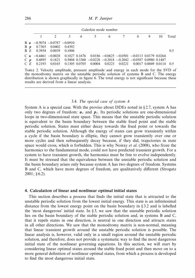
B u −0.5074 −0.0787 −0.0910B p 0.7303 0.0402 0.4392B E 0.3954 0.0039 0.1006 0.5
C u −0.4461 −0.0028 0.1027 0.1676 0.0186 −0.0625 −0.0501 −0.0113 0.0179 0.0264C p 0.4895 0.1821 0.5004 0.3360 −0.0228 −0.2018 −0.2042 −0.0587 0.0980 0.1487C E 0.2193 0.0165 0.1305 0.0705 0.0004 0.0223 0.0221 0.0017 0.0049 0.0114 0.5
Table 2. Velocity amplitude, pressure amplitude and energy in each mode for the SVD ofthe monodromy matrix on the unstable periodic solution of systems B and C. The energydistribution is shown graphically in figure 6. The total energy is not significant because theseresults are derived from a linear analysis.
3.4. The special case of system A
System A is a special case. With the proviso about DDEs noted in § 2.7, system A hasonly two degrees of freedom: u1 and p1. Its periodic solutions are one-dimensionalloops in two-dimensional state space. This means that the unstable periodic solutionis equivalent to the basin boundary between the stable fixed point and the stableperiodic solution. States must either decay towards the fixed point or towards thestable periodic solution. Although the energy of states can grow transiently withina cycle if the basin boundary is elliptic, they cannot grow transiently over one ormore cycles and then subsequently decay because, if they did, trajectories in statespace would cross, which is forbidden. This is why Noiray et al. (2008), who froze theharmonics to the fundamental mode, could not have predicted transient growth. For asystem to have transient growth, the harmonics must be free to evolve independently.It must be stressed that the equivalence between the unstable periodic solution andthe basin boundary arises only because system A has two degrees of freedom. SystemsB and C, which have more degrees of freedom, are qualitatively different (Strogatz2001; § 6.2).
4. Calculation of linear and nonlinear optimal initial statesThis section describes a process that finds the initial state that is attracted to the
unstable periodic solution from the lowest initial energy. This state is an infinitesimaldistance from the lowest energy point on the basin boundary in § 3.2 and is labelledthe ‘most dangerous’ initial state. In § 3, we saw that the unstable periodic solutionlies on the basin boundary of the stable periodic solution and, in systems B and C,that it repels states in one direction, is neutral in one direction and attracts statesin all other directions. We saw that the monodromy matrix is non-normal, meaningthat linear transient growth around the unstable periodic solution is possible. Thelinear analysis is, however, valid only in a small region around the unstable periodicsolution, and therefore, does not provide a systematic way to find the most dangerousinitial state of the nonlinear governing equations. In this section, we will start byconsidering linear optimal states around the stable fixed point and then move on to amore general definition of nonlinear optimal states, from which a process is developedto find the most dangerous initial state.
Triggering in the horizontal Rijke tube 287
0.39
29
0.13
72
0.12
71
1 2 3 4 5 6 7 8 9 100
0.05
0.10
0.15
E
Galerkin mode
System B
1 2 3 4 5 6 7 8 9 100
0.05
0.10
0.15
Galerkin mode
System C
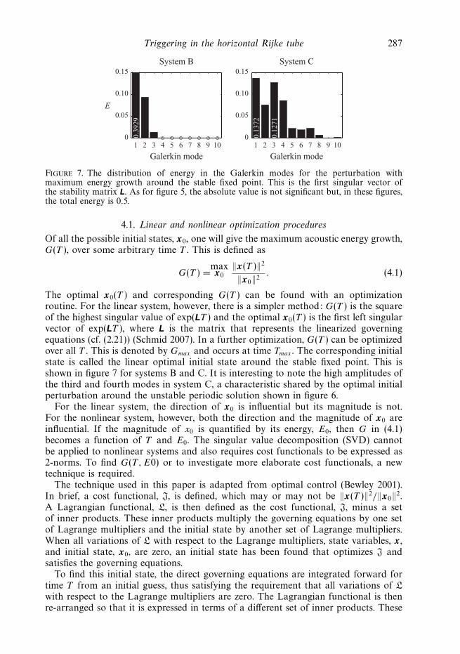
Figure 7. The distribution of energy in the Galerkin modes for the perturbation withmaximum energy growth around the stable fixed point. This is the first singular vector ofthe stability matrix L. As for figure 5, the absolute value is not significant but, in these figures,the total energy is 0.5.
4.1. Linear and nonlinear optimization procedures
Of all the possible initial states, x0, one will give the maximum acoustic energy growth,G(T ), over some arbitrary time T . This is defined as
G(T ) =maxx0
‖x(T )‖2
‖x0‖2. (4.1)
The optimal x0(T ) and corresponding G(T ) can be found with an optimizationroutine. For the linear system, however, there is a simpler method: G(T ) is the squareof the highest singular value of exp(LT ) and the optimal x0(T ) is the first left singularvector of exp(LT ), where L is the matrix that represents the linearized governingequations (cf. (2.21)) (Schmid 2007). In a further optimization, G(T ) can be optimizedover all T . This is denoted by Gmax and occurs at time Tmax . The corresponding initialstate is called the linear optimal initial state around the stable fixed point. This isshown in figure 7 for systems B and C. It is interesting to note the high amplitudes ofthe third and fourth modes in system C, a characteristic shared by the optimal initialperturbation around the unstable periodic solution shown in figure 6.
For the linear system, the direction of x0 is influential but its magnitude is not.For the nonlinear system, however, both the direction and the magnitude of x0 areinfluential. If the magnitude of x0 is quantified by its energy, E0, then G in (4.1)becomes a function of T and E0. The singular value decomposition (SVD) cannotbe applied to nonlinear systems and also requires cost functionals to be expressed as2-norms. To find G(T , E0) or to investigate more elaborate cost functionals, a newtechnique is required.
The technique used in this paper is adapted from optimal control (Bewley 2001).In brief, a cost functional, J, is defined, which may or may not be ‖x(T )‖2/‖x0‖2.A Lagrangian functional, L, is then defined as the cost functional, J, minus a setof inner products. These inner products multiply the governing equations by one setof Lagrange multipliers and the initial state by another set of Lagrange multipliers.When all variations of L with respect to the Lagrange multipliers, state variables, x,and initial state, x0, are zero, an initial state has been found that optimizes J andsatisfies the governing equations.
To find this initial state, the direct governing equations are integrated forward fortime T from an initial guess, thus satisfying the requirement that all variations of L
with respect to the Lagrange multipliers are zero. The Lagrangian functional is thenre-arranged so that it is expressed in terms of a different set of inner products. These
288 M. P. Juniper
inner products multiply the state variables, x, by a first set of constraints. They alsomultiply the initial state, x0, by a second set of constraints. The requirement that allvariations of L with respect to x are zero can be met by satisfying the first constraints.Half of these, known as the optimality conditions, determine the relationship betweenan adjoint state vector, x+, and the direct state vector, x, at time T . The other half,known as the adjoint governing equations, govern the evolution of x+ for t = [0, T ].After setting the optimality conditions at t = T , the adjoint governing equations areintegrated backwards to time 0, thus satisfying the requirement that all variationsof L with respect to x are zero. The second set of constraints return the gradientinformation ∂L/∂x0 at the initial guess for x0. This is combined with a convenientoptimization algorithm, such as the steepest descent method or the conjugate gradientmethod, in order to converge towards the optimal initial state, at which ∂L/∂x0 = 0.
This technique is extremely versatile. It can handle all reasonable cost functionals,boundary conditions and governing equations, either linear or nonlinear. It alsoallows accuracy to be traded for speed by reducing the temporal resolution or thetolerance of the optimization. The adjoint governing equations, optimality conditionsand gradient information are derived for the nonlinear case with cost functional Jav
in Appendix A. For the other cases, these equations are listed without derivation inAppendix B.
4.2. The characteristics of different cost functionals
Several cost functionals would be appropriate for the optimization in this paper, eachwith slightly different adjoint equations. One is the final energy divided by the initialenergy, JT ≡ E(T )/E0, which is equal to G at optimality. Another is the integrated
rate of energy transfer between the thermal and the mechanical field, JpQ ≡∫ T
0pQ dt ,
which is equivalent to JT without including damping. Both of these oscillate with time.Another is the average energy over some specified time window, which also oscillatesunless the time window happens to be exactly equal to one period. Given that thesolution becomes periodic only once the transient behaviour has died away and thatthe period is not necessarily known beforehand, the oscillations cannot, in general,be removed by using this cost functional. Another is the average acoustic energy overt = [0, T ] divided by the initial energy: Jav ≡ Eav(T )/E0. This cost functional increasesmonotonically with time, which is sometimes a useful feature. The cost functionalsJT and Jav are used in this paper.
4.3. Local optimization of the nonlinear governing equations
The local optimization procedure consists of an adjoint looping algorithm and a linemaximization algorithm nested within a conjugate gradient algorithm. The adjointlooping algorithm provides gradient information to the conjugate gradient algorithm.This procedure finds local maxima of J from an initial guess for x0. Two versions ofthe procedure are used. In the first version, no constraints are placed on the initialstate. In the second version, the energy of the initial state, E0, is specified. The secondversion (or some variant of it) is required when the linear governing equations arebeing optimized so that the solution does not grow to infinity or decay to zero.Although the initial energy is irrelevant to the linear solution, allowing it to grow ordecay without constraint can lead to numerical problems. The second version is alsouseful in the global optimization procedures described in § 4.5.
Triggering in the horizontal Rijke tube 289
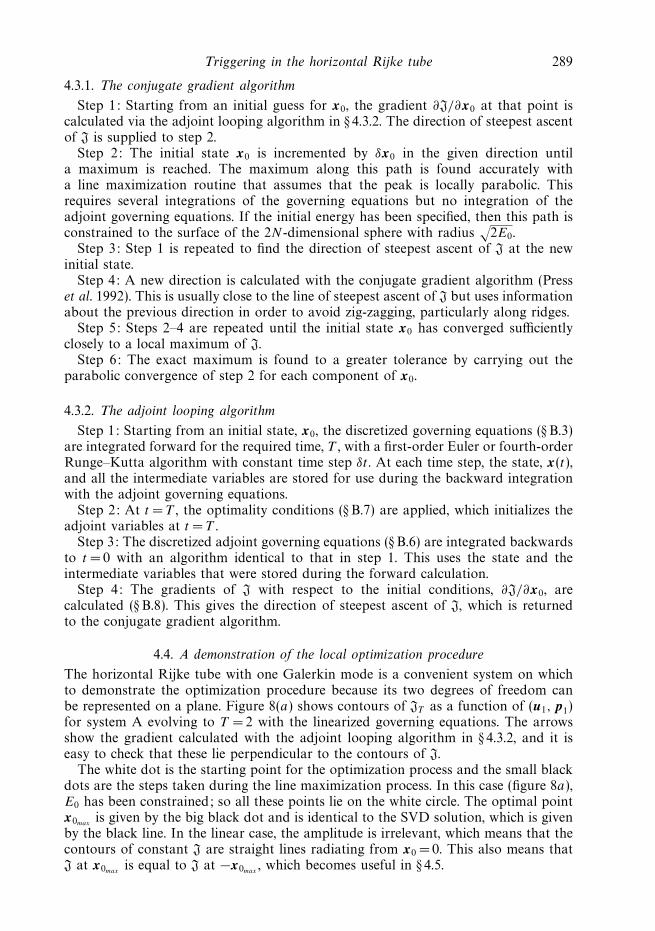
4.3.1. The conjugate gradient algorithm
Step 1: Starting from an initial guess for x0, the gradient ∂J/∂x0 at that point iscalculated via the adjoint looping algorithm in § 4.3.2. The direction of steepest ascentof J is supplied to step 2.
Step 2: The initial state x0 is incremented by δx0 in the given direction untila maximum is reached. The maximum along this path is found accurately witha line maximization routine that assumes that the peak is locally parabolic. Thisrequires several integrations of the governing equations but no integration of theadjoint governing equations. If the initial energy has been specified, then this path isconstrained to the surface of the 2N-dimensional sphere with radius
√2E0.
Step 3: Step 1 is repeated to find the direction of steepest ascent of J at the newinitial state.
Step 4: A new direction is calculated with the conjugate gradient algorithm (Presset al. 1992). This is usually close to the line of steepest ascent of J but uses informationabout the previous direction in order to avoid zig-zagging, particularly along ridges.
Step 5: Steps 2–4 are repeated until the initial state x0 has converged sufficientlyclosely to a local maximum of J.
Step 6: The exact maximum is found to a greater tolerance by carrying out theparabolic convergence of step 2 for each component of x0.
4.3.2. The adjoint looping algorithm
Step 1: Starting from an initial state, x0, the discretized governing equations (§ B.3)are integrated forward for the required time, T , with a first-order Euler or fourth-orderRunge–Kutta algorithm with constant time step δt . At each time step, the state, x(t),and all the intermediate variables are stored for use during the backward integrationwith the adjoint governing equations.
Step 2: At t = T , the optimality conditions (§ B.7) are applied, which initializes theadjoint variables at t = T .
Step 3: The discretized adjoint governing equations (§ B.6) are integrated backwardsto t = 0 with an algorithm identical to that in step 1. This uses the state and theintermediate variables that were stored during the forward calculation.
Step 4: The gradients of J with respect to the initial conditions, ∂J/∂x0, arecalculated (§ B.8). This gives the direction of steepest ascent of J, which is returnedto the conjugate gradient algorithm.
4.4. A demonstration of the local optimization procedure
The horizontal Rijke tube with one Galerkin mode is a convenient system on whichto demonstrate the optimization procedure because its two degrees of freedom canbe represented on a plane. Figure 8(a) shows contours of JT as a function of (u1, p1)for system A evolving to T = 2 with the linearized governing equations. The arrowsshow the gradient calculated with the adjoint looping algorithm in § 4.3.2, and it iseasy to check that these lie perpendicular to the contours of J.
The white dot is the starting point for the optimization process and the small blackdots are the steps taken during the line maximization process. In this case (figure 8a),E0 has been constrained; so all these points lie on the white circle. The optimal pointx0max
is given by the big black dot and is identical to the SVD solution, which is givenby the black line. In the linear case, the amplitude is irrelevant, which means that thecontours of constant J are straight lines radiating from x0 = 0. This also means thatJ at x0max
is equal to J at −x0max, which becomes useful in § 4.5.

290 M. P. Juniper
−0.5 0 0.5 1.0−1.0
−0.5
0
0.5
1.0
p1
p1
(a)
−0.5 0 0.5 1.0−1.0
−0.5
0
0.5
1.0(b)
−0.5 0 0.5 1.0−1.0
−0.5
0
0.5
1.0
u1 u1
(c)
−0.5 0 0.5 1.0−1.0
−0.5
0
0.5
1.0(d )
Figure 8. Contours of cost functional, J(u1, p1), for system A for: (a) J = JT evolving to T = 2with the linear governing equations; (b) J = Jav evolving to T = 2 with the linear governingequations; (c) J = JT evolving to T = 2 with the nonlinear governing equations; (d ) J = Jav
evolving to T =2 with the nonlinear governing equations. The arrows show the gradientscalculated with the adjoint looping algorithm in § 4.3.2. The path of the optimization processdescribed in § 4.3.1 is shown from the initial guess (white dot) to the optimal point (big blackdot). In (a) and (b) the initial energy is fixed. In (c) and (d ) it is unconstrained.
The optimal point can be found to any specified tolerance, although there is atrade-off between the time taken and the accuracy. In the Rijke tube system, forwhich the linear governing equations can be represented by a small matrix (e.g. 20 ×20 for system C), the SVD method is around three orders of magnitude faster thanthe adjoint looping method. In systems that are represented by a large matrix (greaterthan 1000 × 1000), such as that studied by Balasubramanian & Sujith (2008b), theadjoint looping method is faster than the SVD method.
The remaining frames of figure 8 show the same information for (b) cost functionalJav with the linearized governing equations, (c) cost functional JT with the nonlineargoverning equations for unconstrained E0 and (d ) cost functional Jav with thenonlinear governing equations for unconstrained E0. The linear cases are qualitativelysimilar to each other, showing that both cases have unique optimal starting points,x0max
, whether the cost functional be JT , which can be analysed with the SVD method,
Triggering in the horizontal Rijke tube 291
or Jav , which cannot. The nonlinear cases are also qualitatively similar to each otherbut do not have the simple structure of the linear cases. In particular, they each havetwo local maxima, the consequences of which will be discussed in § 4.5.
4.5. Global optimization of the nonlinear governing equations
The conjugate gradient algorithm combined with line maximization and adjointlooping is an efficient way to find local maxima of J. In the linear case, there is asingle maximum. In the nonlinear case, however, there are several local maxima. Thiscan be seen in figures 8(c) and 8(d ) for system A. In systems B and C, there are manymore local maxima.
In this paper, the global maximum is found with a simulated annealing process.Once a local maximum has been found, random perturbations are added to the statevector and new local maxima are sought from these points. Most of these convergeto the original local maximum but, occasionally, a new local maximum is found ina new area. This process continues, with progressively smaller random perturbationsuntil the global maximum is found. The simulated annealing process is robust butslow, and it is highly likely that a more efficient global optimization procedure canbe found.
4.6. Efficient convergence to the most dangerous initial state
The global optimization procedure in § 4.5 can find the initial states with maximumpossible transient growth, G(T , E0), over a wide range of T and E0 (Juniper 2010).The aim of the current paper, however, is to find the state with the lowest initialenergy, E0, that can reach sustained oscillations. This is the state with lowest energyon the basin of attraction of the stable periodic solution. This point can be foundby using the global optimization procedure with cost functional JT = E(T )/E0 overa long time window with unconstrained E0 but this is time-consuming (Juniper &Waugh 2010).
A different procedure is used here. We know from § 3 that all states very close tothe basin boundary start by evolving towards the unstable periodic solution. Thismeans that the optimization needs to be performed only on the first few time units,during which transient growth to the unstable periodic solution takes place. Afterthis period, the evolution from all initial states near the boundary is similar. Anoptimization time of T =10 has been found to be sufficient but T =20 is used inthis paper, corresponding to 10 periods of the first mode’s natural frequency. If theoptimization period is too short, the initial state with highest transient growth can beone that subsequently decays very quickly.
The optimization procedure starts from the lowest energy point on the unstableperiodic solution because this is the lowest energy point on the basin boundary thatcan be found with the continuation method. There is no transient growth around thecycle when starting from this point. The global optimization process then finds a statethat has the same initial energy but that maximizes transient growth over 20 timeunits. Its amplitude is then reduced incrementally and the evolution calculated wellbeyond the period of transient growth. This is repeated until the initial energy is foundat which the state evolves to the unstable periodic solution but then neither growsnor decays over several hundred time units. This point is extremely close to the basinof attraction of the stable periodic solution and has lower energy than the previouspoint but is not necessarily the most dangerous initial state. The optimization process
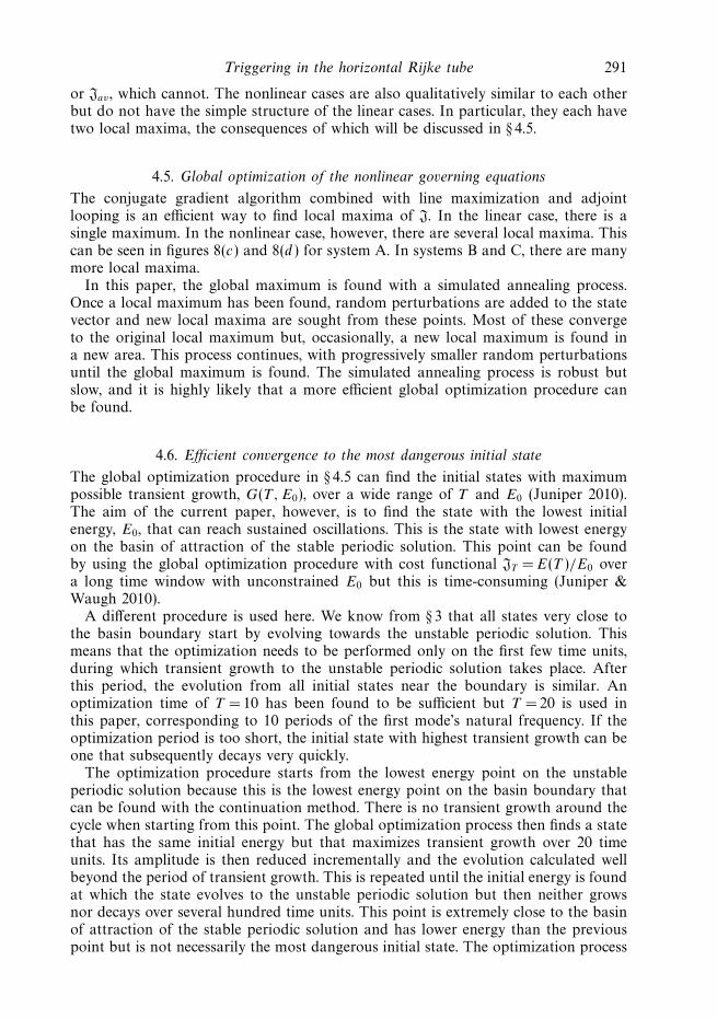
292 M. P. Juniper
Galerkin mode number
1 2 3 4 5 6 7 8 9 10 Total
B u −0.3715 −0.0040 −0.0331B p −0.0356 0.0112 0.0005B E 0.0696 0.0001 0.0005 0.0702
C u −0.4334 −0.0321 −0.1298 −0.0596 −0.0009 −0.0035 0.0146 0.0063 0.0025 0.0301C p −0.0813 0.0191 0.0021 −0.0353 −0.0004 −0.0025 0.0006 0.0072 −0.0178 −0.0101C E 0.0972 0.0007 0.0084 0.0024 0.0000 0.0000 0.0001 0.0000 0.0001 0.0005 0.1096
Table 3. Velocity amplitude, pressure amplitude and energy in each mode for the mostdangerous initial state of systems B and C. The energy, E, is shown graphically in figure 9.The total energy is shown in the final column. It is significantly lower than the energy of thelowest energy point on the unstable periodic solution in table 1.
0
1
2
3
4
E
0.06
965
0.09
723
0.00
8429
1 2 3 4 5 6 7 8 9 10
(×10−3)
Galerkin mode
System B
0
1
2
3
4
1 2 3 4 5 6 7 8 9 10
(×10−3)
Galerkin mode
System C
Figure 9. The distribution of energy in the Galerkin modes for the most dangerous initialstates for systems B and C, found with the optimization procedure in § 4. The absolute valuesare significant because this is derived from a nonlinear analysis. The exact distribution ofu, p and E is in table 3. These states lie just within the basin of attraction of the stableperiodic solution. As expected from the first singular value of the monodromy matrix infigure 6, system B has significant energy in the third mode and system C has significant energyin the third and fourth modes in order that these initial states can maximize their energygrowth around the unstable periodic solution.
and the energy reduction process are repeated in sequence until any further reductionin the energy is less than 10−4.
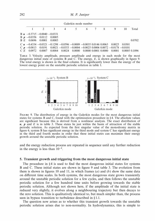
5. Transient growth and triggering from the most dangerous initial stateThe procedure in § 4 is used to find the most dangerous initial states for systems
B and C. These initial states are shown in figure 9 and table 3. The evolution fromthem is shown in figures 10 and 11, in which frames (a) and (b) show the same dataon different time scales. In both systems, the most dangerous state grows transientlyaround the unstable periodic solution for a few cycles, and then follows the unstableperiodic solution for a few hundred time units before growing towards the stableperiodic solution. Although not shown here, if the amplitude of the initial state isreduced very slightly, it evolves along a neighbouring trajectory but then decays tothe zero solution. This is qualitatively identical to, but much simpler than, the processseen in bypass transition to turbulence described in § 1.1.
The question now arises as to whether this transient growth towards the unstableperiodic solution arises due to non-normality. In hydrodynamics, this is simple to

Triggering in the horizontal Rijke tube 293
2 4 6 8 100
0.05
0.10
0.15
0.20
0.25
0.05
0.10
0.15
0.20
0.25
t t
E 0 2
0 200 400 600 800 1000
Figure 10. Evolution with the nonlinear governing equations from the most dangerous initialstate of system B (grey line). The energy of the system grows transiently over the first few cycles,then follows the unstable periodic solution (dashed line) for several cycles, before growing tothe stable periodic solution.
2 4 6 8 100
0.05
0.10
0.15
0.20
0.25
0.05
0.10
0.15
0.20
0.25
t t
E
0 200 400 600 800 1000
Figure 11. As for figure 10 but for system C. The transient growth is stronger in system C.Although this state evolves to the stable periodic solution earlier than system B, this is notsignificant because the time spent around the unstable periodic solution is extremely sensitiveto tiny variations in the amplitude of the initial state.
answer because the nonlinear terms conserve energy, meaning that any energy growthmust be due to linear terms and, if all eigenvalues are linearly stable, must therefore bedue to non-normality. In thermoacoustics, however, the nonlinearity does not conserveenergy and could cause transient growth even in the absence of non-normality.
We know, however, from § 3.3 that the monodromy matrix of the unstable periodicsolution is non-normal and that this causes linear transient growth around theunstable periodic solution. Furthermore, the linear perturbations that cause the highesttransient energy growth have highest amplitudes in the first, third and fourth modes(in the first and third modes for system B). This characteristic is shared by thenonlinear most dangerous initial states. This strongly suggests that transient growthin the nonlinear system is also due to linear non-normality. Further evidence isprovided in figure 12. This shows the evolution from the most dangerous initial statefor system C, using the governing equations linearized around the stable fixed point(see (2.19)–(2.20)). The first point to note, by comparing this linear evolution withthe unstable periodic solution (dashed line), is that the initial energy growth of thelinear evolution exceeds that of the unstable periodic solution. Put together with theresults from the monodromy matrix, this shows that transient growth arises fromthe linear part of the evolution operator, whether this operator is linearized aboutthe stable fixed point or around the unstable periodic solution. The second point tonote, by comparing the linear evolution (solid line in figure 12) with the nonlinearevolution (solid line in figure 11), is that the nonlinear system has larger transient
294 M. P. Juniper
Emax − Emin = 0.0366
Emax − Emin = 0.0412
2 4 6 8 100
0.05
0.10
0.15
0.20
0.25
0.05
0.10
0.15
0.20
0.25
t t
E
0 200 400 600 800 1000
Figure 12. Evolution with the linear governing equations from the optimal initial point ofsystem C (black line), showing transient growth at the very beginning but then decay to thestable fixed point at zero, which is the only solution of the linear governing equations. Thisshows that the linear transient growth from this point exceeds that which is achieved fromstarting at the minimum energy point of the unstable periodic solution (dashed line).
growth than the linear system. This shows that, around the unstable periodic solution,both nonlinearity and non-normality contribute to transient growth. The same resulthas been found for transient growth around the stable fixed point (Juniper 2010). Onthis feature, thermoacoustic systems differ from hydrodynamic systems.
It is worth pointing out that the linear optimal state around the stable fixedpoint, shown in figure 7, differs significantly from the most dangerous initial state.Although, for system C, both have high energies in the third and fourth modes, themost dangerous initial state has much higher energy in the first mode in order for itto start near the unstable periodic solution. At the energies required for triggering,the linear optimal around the stable fixed point has little transient growth. This isdescribed in detail in Juniper (2010).
In summary, the most dangerous initial state has been found by embeddingnonlinear adjoint looping within a conjugate gradient algorithm. This is a brute forceapproach that makes no assumptions about the mechanisms of transient growth. It isseen that this initial state exploits linear transient growth around the unstable periodicsolution in order to be attracted initially towards the unstable periodic solution and,from there, towards the stable periodic solution. This is directly analogous to stages2–4 in bypass transition to turbulence (§ 1.1). There are, however, some differencesbetween triggering in thermoacoustics and bypass transition in hydrodynamics.Firstly, nonlinearity (as well as non-normality) contributes to transient growth inthermoacoustics. Secondly, at least in this simple thermoacoustic model, the basinboundary contains only one unstable periodic solution while, in hydrodynamics, itcontains several.
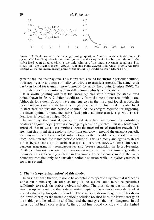
6. The ‘safe operating region’ of this modelIn an industrial situation, it would be acceptable to operate a system that is ‘linearly
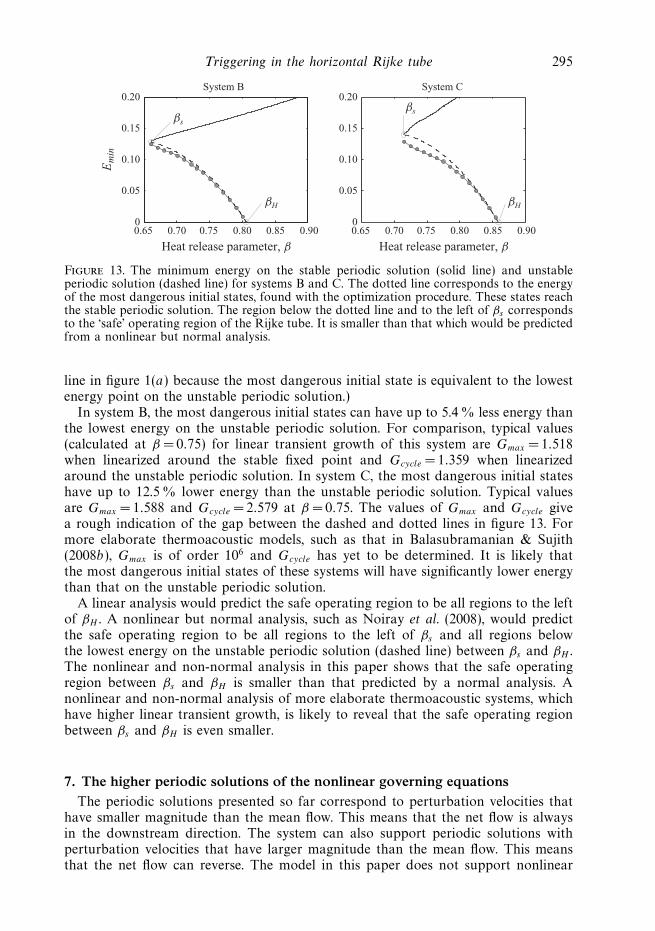
stable but nonlinearly unstable’ as long as the system could never be perturbedsufficiently to reach the stable periodic solution. The most dangerous initial statesgive the upper bound of this ‘safe operating region’. These have been calculated atseveral values of β for systems B and C. The results are shown in figure 13. This showsthe lowest energy on the unstable periodic solution (dashed line), the lowest energy onthe stable periodic solution (solid line) and the energy of the most dangerous initialstates (dotted line). (For system A, the dotted line would coincide with the dashed
Triggering in the horizontal Rijke tube 295
0.65 0.70 0.75 0.80 0.85 0.900
0.05
0.10
0.15
0.20
Heat release parameter, β
Em
in
0.65 0.70 0.75 0.80 0.85 0.900
0.05
0.10
0.15
0.20
Heat release parameter, β
βH
βs
System B System C
βH
βs
Figure 13. The minimum energy on the stable periodic solution (solid line) and unstableperiodic solution (dashed line) for systems B and C. The dotted line corresponds to the energyof the most dangerous initial states, found with the optimization procedure. These states reachthe stable periodic solution. The region below the dotted line and to the left of βs correspondsto the ‘safe’ operating region of the Rijke tube. It is smaller than that which would be predictedfrom a nonlinear but normal analysis.
line in figure 1(a) because the most dangerous initial state is equivalent to the lowestenergy point on the unstable periodic solution.)
In system B, the most dangerous initial states can have up to 5.4 % less energy thanthe lowest energy on the unstable periodic solution. For comparison, typical values(calculated at β = 0.75) for linear transient growth of this system are Gmax =1.518when linearized around the stable fixed point and Gcycle = 1.359 when linearizedaround the unstable periodic solution. In system C, the most dangerous initial stateshave up to 12.5 % lower energy than the unstable periodic solution. Typical valuesare Gmax = 1.588 and Gcycle =2.579 at β = 0.75. The values of Gmax and Gcycle givea rough indication of the gap between the dashed and dotted lines in figure 13. Formore elaborate thermoacoustic models, such as that in Balasubramanian & Sujith(2008b), Gmax is of order 106 and Gcycle has yet to be determined. It is likely thatthe most dangerous initial states of these systems will have significantly lower energythan that on the unstable periodic solution.
A linear analysis would predict the safe operating region to be all regions to the leftof βH . A nonlinear but normal analysis, such as Noiray et al. (2008), would predictthe safe operating region to be all regions to the left of βs and all regions belowthe lowest energy on the unstable periodic solution (dashed line) between βs and βH .The nonlinear and non-normal analysis in this paper shows that the safe operatingregion between βs and βH is smaller than that predicted by a normal analysis. Anonlinear and non-normal analysis of more elaborate thermoacoustic systems, whichhave higher linear transient growth, is likely to reveal that the safe operating regionbetween βs and βH is even smaller.
7. The higher periodic solutions of the nonlinear governing equationsThe periodic solutions presented so far correspond to perturbation velocities that
have smaller magnitude than the mean flow. This means that the net flow is alwaysin the downstream direction. The system can also support periodic solutions withperturbation velocities that have larger magnitude than the mean flow. This meansthat the net flow can reverse. The model in this paper does not support nonlinear

296 M. P. Juniper
0 0.5 1.0 1.5 2.010–2
10–1
100
101
102
Em
in
Heat release parameter, β
System B
0 0.5 1.0 1.5 2.010–2
10–1
100
101
102
Heat release parameter, β
System C
Figure 14. The minimum energy on the stable periodic solution (solid lines) and unstableperiodic solution (dashed lines) for systems B and C. The dotted lines correspond to the energyof the most dangerous initial states, found with the optimization procedure. These states reachthe stable periodic solution above them.
10 20 30 400
0.5
1.0
1.5
t t
E
E
200 400 600 800 10000
10
20
30
40
50
0
0.05
0.10
0.15
0.20
Galerkin mode1 2 3 4 5 6 7 8 9 101 2 3 4 5 6 7 8 9 10
0
0.1
0.2
0.3
0.4
Galerkin mode1 2 3 4 5 6 7 8 9 10
Galerkin mode
t = 0
0.57
73
t = 20
1.23
3
0
2
4
6
8
10
t = 1000
25.5
3
Figure 15. As for figure 10 but for the higher periodic solutions of system B. The distributionof energy in the Galerkin modes is shown at the start (t = 0), on the upper unstable periodicsolution (t = 20 and dashed line) and on the upper stable periodic solution (t =1000). On thebar charts, the vertical axes are scaled to 25 % of the amplitude of the first mode.
acoustics, which may well be influential in this range. Nevertheless, these results areworth reporting, even if they are only qualitatively correct.
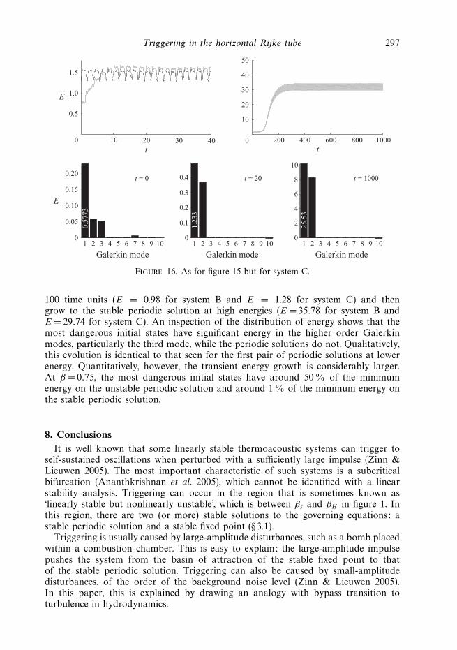
The second pair of periodic solutions, one unstable and one stable, are shown infigure 14 for systems B and C. Log scales are used because the energy is much higherthan that of the first pair of periodic solutions. The most dangerous initial statesthat can reach these periodic solutions (dotted line) lie at significantly lower energythan that of the unstable periodic solution. Figures 15 and 16 show time evolutionsfrom the most dangerous initial conditions at β = 0.75. They start from low energies(E0 = 0.6013 for system C and E0 = 0.7026 for system C), grow transiently over5–10 time units, are attracted towards the unstable periodic solutions for around
Triggering in the horizontal Rijke tube 297
0
0.5
1.0
1.5
200 400 600 800 10000
10
20
30
40
50
t
1 2 3 4 5 6 7 8 9 100
0.05
0.10
0.15
0.20
Galerkin mode1 2 3 4 5 6 7 8 9 10
Galerkin mode1 2 3 4 5 6 7 8 9 10
Galerkin mode
t = 0
0.57
73
0
0.1
0.2
0.3
0.4 t = 20
1.23
3
0
2
4
6
8
10
t = 1000
25.5
3
10 20 30 40t
E
E
Figure 16. As for figure 15 but for system C.
100 time units (E = 0.98 for system B and E = 1.28 for system C) and thengrow to the stable periodic solution at high energies (E = 35.78 for system B andE = 29.74 for system C). An inspection of the distribution of energy shows that themost dangerous initial states have significant energy in the higher order Galerkinmodes, particularly the third mode, while the periodic solutions do not. Qualitatively,this evolution is identical to that seen for the first pair of periodic solutions at lowerenergy. Quantitatively, however, the transient energy growth is considerably larger.At β =0.75, the most dangerous initial states have around 50 % of the minimumenergy on the unstable periodic solution and around 1 % of the minimum energy onthe stable periodic solution.
8. ConclusionsIt is well known that some linearly stable thermoacoustic systems can trigger to
self-sustained oscillations when perturbed with a sufficiently large impulse (Zinn &Lieuwen 2005). The most important characteristic of such systems is a subcriticalbifurcation (Ananthkrishnan et al. 2005), which cannot be identified with a linearstability analysis. Triggering can occur in the region that is sometimes known as‘linearly stable but nonlinearly unstable’, which is between βs and βH in figure 1. Inthis region, there are two (or more) stable solutions to the governing equations: astable periodic solution and a stable fixed point (§ 3.1).
Triggering is usually caused by large-amplitude disturbances, such as a bomb placedwithin a combustion chamber. This is easy to explain: the large-amplitude impulsepushes the system from the basin of attraction of the stable fixed point to thatof the stable periodic solution. Triggering can also be caused by small-amplitudedisturbances, of the order of the background noise level (Zinn & Lieuwen 2005).In this paper, this is explained by drawing an analogy with bypass transition toturbulence in hydrodynamics.
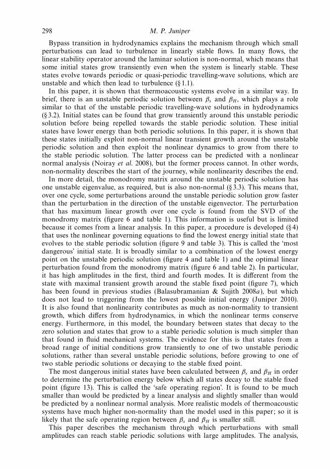
298 M. P. Juniper
Bypass transition in hydrodynamics explains the mechanism through which smallperturbations can lead to turbulence in linearly stable flows. In many flows, thelinear stability operator around the laminar solution is non-normal, which means thatsome initial states grow transiently even when the system is linearly stable. Thesestates evolve towards periodic or quasi-periodic travelling-wave solutions, which areunstable and which then lead to turbulence (§ 1.1).
In this paper, it is shown that thermoacoustic systems evolve in a similar way. Inbrief, there is an unstable periodic solution between βs and βH , which plays a rolesimilar to that of the unstable periodic travelling-wave solutions in hydrodynamics(§ 3.2). Initial states can be found that grow transiently around this unstable periodicsolution before being repelled towards the stable periodic solution. These initialstates have lower energy than both periodic solutions. In this paper, it is shown thatthese states initially exploit non-normal linear transient growth around the unstableperiodic solution and then exploit the nonlinear dynamics to grow from there tothe stable periodic solution. The latter process can be predicted with a nonlinearnormal analysis (Noiray et al. 2008), but the former process cannot. In other words,non-normality describes the start of the journey, while nonlinearity describes the end.
In more detail, the monodromy matrix around the unstable periodic solution hasone unstable eigenvalue, as required, but is also non-normal (§ 3.3). This means that,over one cycle, some perturbations around the unstable periodic solution grow fasterthan the perturbation in the direction of the unstable eigenvector. The perturbationthat has maximum linear growth over one cycle is found from the SVD of themonodromy matrix (figure 6 and table 1). This information is useful but is limitedbecause it comes from a linear analysis. In this paper, a procedure is developed (§ 4)that uses the nonlinear governing equations to find the lowest energy initial state thatevolves to the stable periodic solution (figure 9 and table 3). This is called the ‘mostdangerous’ initial state. It is broadly similar to a combination of the lowest energypoint on the unstable periodic solution (figure 4 and table 1) and the optimal linearperturbation found from the monodromy matrix (figure 6 and table 2). In particular,it has high amplitudes in the first, third and fourth modes. It is different from thestate with maximal transient growth around the stable fixed point (figure 7), whichhas been found in previous studies (Balasubramanian & Sujith 2008a), but whichdoes not lead to triggering from the lowest possible initial energy (Juniper 2010).It is also found that nonlinearity contributes as much as non-normality to transientgrowth, which differs from hydrodynamics, in which the nonlinear terms conserveenergy. Furthermore, in this model, the boundary between states that decay to thezero solution and states that grow to a stable periodic solution is much simpler thanthat found in fluid mechanical systems. The evidence for this is that states from abroad range of initial conditions grow transiently to one of two unstable periodicsolutions, rather than several unstable periodic solutions, before growing to one oftwo stable periodic solutions or decaying to the stable fixed point.
The most dangerous initial states have been calculated between βs and βH in orderto determine the perturbation energy below which all states decay to the stable fixedpoint (figure 13). This is called the ‘safe operating region’. It is found to be muchsmaller than would be predicted by a linear analysis and slightly smaller than wouldbe predicted by a nonlinear normal analysis. More realistic models of thermoacousticsystems have much higher non-normality than the model used in this paper; so it islikely that the safe operating region between βs and βH is smaller still.
This paper describes the mechanism through which perturbations with smallamplitudes can reach stable periodic solutions with large amplitudes. The analysis,
Triggering in the horizontal Rijke tube 299
however, assumes that a perfectly defined impulse can be imposed onto a perfectlyquiet system, which is unrealistic. It is more realistic to examine the effect of continuousnoise on a non-normal system. In Waugh & Juniper (2010), noise with spectralcharacteristics similar to the most dangerous initial state is imposed onto the modelused in this paper. The noise amplitude is increased until the system triggers tothe stable periodic solution. The triggering process follows exactly that which isexpected from this paper: the system starts around the stable fixed point, then jumpsto the unstable periodic solution and then grows to the stable periodic solution.This compares well with experimental results of low-amplitude triggering such asfigure 15(b) of Lieuwen (2002).
From an engineering point of view, it is important to know whether non-normalityand transient growth are likely to be influential in triggering self-sustained oscillationsin real thermoacoustic systems. Real thermoacoustic systems have transient growththat is several orders of magnitude higher than that in a Rijke tube. With sufficientcomputing power, the techniques presented in this paper could be used to calculatethe safe operating regions of more accurate models of thermoacoustic systems. Evenwithout this step, however, one practical conclusion of this study is that, in systemsthat are linearly stable, one must look for nonlinear self-sustained oscillations becauseit may take surprisingly little initial energy for the system to find a way to reach them.
I would like to thank P. Schmid for patiently helping at numerous stages duringthis project, particularly with implementation of the nonlinear adjoint looping andconjugate gradient algorithms. I am very grateful to R. I. Sujith and S. Nagaraja forhelpful and enthusiastic discussions from the start of this project and for providingthe Matlab code that they used in Balasubramanian & Sujith (2008a). I would liketo thank S. Mariappan and P. Subramanian for introducing me to DDE-Biftool andI. Waugh and M. Geuss for mastering it. I would also like to thank A. Bottaro forexplaining the principles of nonlinear adjoint looping, and P. Huerre and P. Schmidfor their very clear notes on Optimal Control. This work was supported by EPSRCand the Advanced Instability Methods (AIM) Network under grants EP/G033803/1and EP/GO37779/1.
Appendix A. Constrained optimizationIn this appendix, the equations for constrained optimization are derived for
the continuous nonlinear governing equations with cost functional Jav ≡ Eav/E0.Appendix B contains all other variations of these equations: for linear and nonlineargoverning equations; in continuous and discrete form; and for cost functionals Jav
and JT .
A.1. Definitions
The following inner products are defined:
〈g, h〉 ≡ 1
X
∫ X
0
gh dx, (A 1)
{g, h} ≡ 1
T
∫ T
0
gh dt, (A 2)
[g, h] ≡ 1
XT
∫ X
0
∫ T
0
gh dt dx. (A 3)

300 M. P. Juniper
The cost functional is defined as the mean acoustic energy during time T divided bythe initial acoustic energy:
J ≡ Eav
E0
=[u, u] + [p, p]
〈u0, u0〉 + 〈p0, p0〉 . (A 4)
The variation of J with respect to variation in u, for instance, is defined as[∂J
∂u, δu
]≡ lim
ε→0
J(u + εδu) − J(u)
ε. (A 5)
A.2. The direct governing equations in continuous form
The delayed velocity v(x, t) ≡ u(x, t − τ ) is introduced into the governing equations(2.5) and (2.6) in order to separate the time delay term from the nonlinear term. Thisis not strictly necessary but it makes the derivation easier to present. The governingequations for u(x, t) and p(x, t) and the initial conditions for u(x, 0) and p(x, 0) arewritten in terms of functions that equal zero:
F1(x, t) ≡ ∂u
∂t+
∂p
∂x= 0, (A 6)
F2(x, t) ≡ ∂p
∂t+
∂u
∂x+ ζp − β
( ∣∣∣∣13 + vf
∣∣∣∣1/2
−(
1
3
)1/2 )δD(x − xf ) = 0, (A 7)
F3(x, t) ≡ v − u(t − τ ) = 0, (A 8)
G1(x) ≡ u(0) − u0 = 0, (A 9)
G2(x) ≡ p(0) − p0 = 0. (A 10)
Equations (A 9) and (A 10) are not necessary for the derivation of the adjointequations but are included so that it is easier to extract the change in the costfunctional with respect to changes in the initial conditions.
A.3. Definition and re-arrangement of the Lagrangian functional
The cost functional J is to be maximized subject to the constraints (A 6)–(A 10). Toachieve this, a Lagrangian functional, L, is defined with Lagrange multipliers a(x, t),b(x, t), c(x, t), d(x) and e(x):
L ≡ J − [a, F1] − [b, F2] − [c, F3] − 〈d, G1〉 − 〈e, G2〉. (A 11)
At optimality, the variations of L with respect to variations in all of the variablesmust be zero.
The variations of L with respect to variations in a, b, c, d and e are automaticallyzero if the governing equations (A 6)–(A 8) are satisfied for x = [0, X] and t = [0, T ]and if the initial conditions (A 9)–(A 10) are satisfied for x = [0, X] at t = 0.
The variations of L with respect to variations in u, p, v, u0 and p0 are calculatedby re-arranging the terms on the right-hand side of (A 11). The contributions of thenonlinear terms in (A 11) are considered first.
One nonlinear term arises from J. Following the definition (A 5), the variations inJ with respect to variations in u, p, u0 and p0 are[
∂J
∂u, δu
]=
1
ε
(1
XT
∫ T
0
∫ X
0
(u + εδu)2
2E0
dx dt − 1
XT
∫ T
0
∫ X
0
u2
2E0
dx dt
)
=1
XT
∫ T
0
∫ X
0
2u
2E0
δu dx dt =
[u
E0
, δu
], (A 12)
Triggering in the horizontal Rijke tube 301[∂J
∂p, δp
]=
[p
E0
, δp
], (A 13)[
∂J
∂u0
, δu0
]=
[−u0Eav
E20
, δu0
], (A 14)[
∂J
∂p0
, δp0
]=
[−p0Eav
E20
, δp0
], (A 15)
where 2E0 ≡ 〈u0, u0〉 + 〈p0, p0〉 and 2Eav ≡ [u0, u0] + [p0, p0].Another nonlinear term arises from [b, F2]. The contribution to L of this term,
which is briefly labelled K, is
K ≡ −[b, −βδD(x − xf )
(∣∣ 13
+ vf
∣∣1/2 −(
13
)1/2)]
. (A 16)
The variation of K with respect to variations in v(x, t) is to be calculated, using thefact that (
13
+ (vf + εδvf ))1/2
=(
13
+ vf
)1/2+ 1
2
(13
+ vf
)−1/2εδvf , (A 17)
for infinitesimal ε, where δvf is the variation of v evaluated at the hot wire position:
δvf ≡∫ X
0
δv δD(x − xf ) dx. (A 18)
As a reminder, δ represents a small variation and δD represents the Dirac delta. Forvf � −1/3, the variation of K is[
∂K
∂v, δv
]≡ lim
ε→0
K(v + εδv) − K(v)
ε
= −[b, −βδD(x − xf )
1
2
(1
3+ vf
)−1/2
δvf
]
=1
XT
∫ X
0
∫ T
0
βbδD(x − xf )1
2
(1
3+ vf
)−1/2
δvf dt dx
=1
XT
∫ T
0
βbf
1
2
(1
3+ vf
)−1/2
δvf dt
=1
XT
∫ T
0
βbf
1
2
(1
3+ vf
)−1/2 ∫ X
0
δv δD(x − xf ) dx dt
=1
XT
∫ T
0
∫ X
0
βbf
1
2
(1
3+ vf
)−1/2
δv δD(x − xf ) dx dt
=
[βbf
1
2
(1
3+ vf
)−1/2
δD(x − xf ), δv
]. (A 19)
For vf < −1/3, the gradient changes sign due to the modulus in (A 16). To handle this,a sign function, σ , is placed in front of β in (A 19) such that σ =+1 for vf � −1/3and σ = −1 for vf < −1.3. There are no more nonlinear terms.
The contributions of the linear terms in (A 11) are considered next. The innerproducts in terms of a, b, c, d and e are expanded, integrated by parts, re-arranged
302 M. P. Juniper
and expressed as inner products in terms of u, p, v, u0 and p0:
− [a, F1] = − 1
XT
∫ X
0
∫ T
0
a∂u
∂tdt dx − 1
XT
∫ X
0
∫ T
0
a∂p
∂xdt dx
= − 1
XT
∫ X
0
(a(T )u(T ) − a(0)u(0)) dx +1
XT
∫ X
0
∫ T
0
u∂a
∂tdt dx · · ·
− 1
XT
∫ T
0
(p(X)a(X) − p(0)a(0)) dt +1
XT
∫ X
0
∫ T
0
p∂a
∂xdt dx
= −⟨
a(T )
T, u(T )
⟩+
⟨a(0)
T, u(0)
⟩+
[∂a
∂t, u
]· · ·
−{
a(X)
X, p(X)
}+
{a(0)
X, p(0)
}+
[∂a
∂x, p
]. (A 20)
− [b, F2] = −⟨
b(T )
T, p(T )
⟩+
⟨b(0)
T, p(0)
⟩+
[∂b
∂t, p
]· · ·
−{
b(X)
X, u(X)
}+
{b(0)
X, u(0)
}+
[∂b
∂x, u
]− [ζb, p], (A 21)
− [c, F3] = − [c, v] + [c, u(t − τ )], (A 22)
−〈d, G1〉 = −〈d, u(0)〉 + 〈d, u0〉, (A 23)
−〈e, G2〉 = −〈e, p(0)〉 + 〈e, p0〉. (A 24)
The last term in (A 22) needs to be expressed in terms of u(t), rather than u(t − τ ),before it can be combined with the other terms. This is achieved with a change ofvariable t ′ ≡ t − τ and a change in the limits of the time integration:
[c, u(t − τ )] =1
XT
∫ T
0
∫ X
0
c(t)u(t − τ ) dx dt
=1
XT
∫ T −τ
−τ
∫ X
0
c(t ′ + τ )u(t ′) dx dt ′
=1
XT
∫ 0
−τ
∫ X
0
c(t ′ + τ )u(t ′) dx dt ′ +1
XT
∫ T −τ
0
∫ X
0
c(t ′ + τ )u(t ′) dx dt ′
= [c(t + τ ), u]0−τ + [c(t + τ ), u]T −τ0 + [0, u]TT −τ . (A 25)
The boundary conditions for pressure require that p(X) = p(0) = 0 and the boundaryconditions for adjoint pressure require that b(X) = b(0) = 0; so the terms in curlybraces in (A 20) and (A 21) are zero.
For the linear terms, the variations can be written down by inspection. (For example,in (A 20) u is simply replaced with δu.) Gathering together all the contributions from(A 12)–(A 15) and (A 19)–(A 25) gives[
∂L
∂u, δu
]=
[(u
E0
+∂a
∂t+
∂b
∂x+ c(t + τ )
), δu
]T −τ
0
+
[(u
E0
+∂a
∂t+
∂b
∂x
), δu
]T
T −τ
· · ·
+ [c(t + τ ), δu]0−τ −⟨
a(T )
T, δu(T )
⟩+
⟨(a(0)
T− d
), δu(0)
⟩, (A 26)
[∂L
∂p, δp
]=
[(p
E0
+∂b
∂t+
∂a
∂x− ζb, δp
)]T
0
−⟨
b(T )
T, δp(T )
⟩+
⟨b(0)
T− e, δp(0)
⟩,
(A 27)
Triggering in the horizontal Rijke tube 303[∂L
∂v, δv
]=
[σβbf
1
2
(1
3+ vf
)−1/2
δD(x − xf ) − c, δv
]T
0
, (A 28)⟨∂L
∂u0
, δu0
⟩=
⟨d − u0Eav
E20
, δu0
⟩, (A 29)⟨
∂L
∂p0
, δp0
⟩=
⟨e − p0Eav
E20
, δp0
⟩. (A 30)
A.4. The adjoint governing equations in continuous form
At optimality, (A 26)–(A 30) must equal zero for any δu, δp and δv. This leads to theoptimality conditions, which will be presented in the next section, and the adjointgoverning equations, which must be satisfied for x = [0, x] and t =[0, T ]:
bf = 0, for t = [0, τ ], (A 31)
F +1 ≡ ∂a
∂t+
∂b
∂x+
u
E0
+ σβbf (t + τ )1
2· · ·
×(
1
3+ uf (t)
)−1/2
δD(x − xf ) = 0, for t = [0, T − τ ], (A 32)
F +1 ≡ ∂a
∂t+
∂b
∂x+
u
E0
= 0, for t = (T − τ, T ], (A 33)
F +2 ≡ ∂b
∂t+
∂a
∂x+
p
E0
− ζb = 0, for t =[0, T ]. (A 34)
A.5. The optimality conditions at t = 0 and t = T
Similarly, the requirement that (A 26)–(A 30) must equal zero for any δu, δp and δv
leads to the optimality condition at t = T :
a(T ) = 0, b(T ) = 0, (A 35)
which can be thought of as the initialization of the adjoint variables It also leads toan optimality condition at t = 0, which is later used to find gradient information:
d =a(0)
T, e =
b(0)
T. (A 36)
A.6. Gradient information
The gradient information ∂L/∂u0 and ∂L/∂p0 is found by combining (A 29) and(A 30) with (A 36):
∂L
∂u0
=a(0)
T− Eav
E20
u0, (A 37)
∂L
∂p0
=b(0)
T− Eav
E20
p0. (A 38)
If (A 31)–(A 35) are satisfied, then ∂J/∂u0 = ∂L/∂u0 and ∂J/∂p0 = ∂L/∂p0, subjectto the constraints, which means that (A 37) and (A 38) give gradient informationabout J with respect to the initial conditions u0 and p0. This information is used ina convenient optimization routine in order to find the point where ∂J/∂u0 = 0 and∂J/∂p0 = 0, subject to the constraints, which is the optimal point.
304 M. P. Juniper
Appendix B. Catalogue of all the equations required for optimizationThis appendix contains the direct governing equations, adjoint governing equations,
optimality conditions and gradient information for the Rijke tube in the followingcases: linear and nonlinear; continuous and discrete; cost functionals Jav and JT .
B.1. Definitions
Inner products:
〈g, h〉 ≡ 1
X
∫ X
0
gh dx, {g, h} ≡ 1
T
∫ T
0
gh dt, [g, h] ≡ 1
XT
∫ X
0
∫ T
0
gh dt dx.
(B 1)
Cost functionals:
Jav ≡ Eav
E0
=[u, u] + [p, p]
〈u0, u0〉 + 〈p0, p0〉 , JT ≡ ET
E0
=〈u, u〉 + 〈p, p〉
〈u0, u0〉 + 〈p0, p0〉 . (B 2)
Basis sets for discretization:
u =
N∑j=1
ηj cos(jπx), p = −N∑
j=1
(ηj
jπ
)sin(jπx). (B 3)
The variables a and b, respectively, represent the adjoint velocity and pressure andhave the same boundary conditions as u and p, respectively. They are discretized ina way similar to u and p:
a =
N∑j=1
(ξj
jπ
)cos(jπx), b = −
N∑j=1
νj sin(jπx). (B 4)
The following abbreviations are defined: sj ≡ sin(jπxf ) and cj ≡ cos(jπxf ).
B.2. Direct governing equations in continuous form
Nonlinear:
F1 ≡ ∂u
∂t+
∂p
∂x= 0, (B 5)
F2 ≡ ∂p
∂t+
∂u
∂x+ ζp − β
( ∣∣∣∣13 + uf (t − τ )
∣∣∣∣1/2
−(
1
3
)1/2 )δD(x − xf ) = 0. (B 6)
Linear:
F1 ≡ ∂u
∂t+
∂p
∂x= 0, (B 7)
F2 ≡ ∂p
∂t+
∂u
∂x+ ζp − β
√3
2
(uf − τ
∂uf
∂t
)δD(x − xf ) = 0. (B 8)
B.3. Direct governing equations in discrete form
Nonlinear:
F1G ≡ d
dtηj − jπ
(ηj
jπ
)= 0, (B 9)
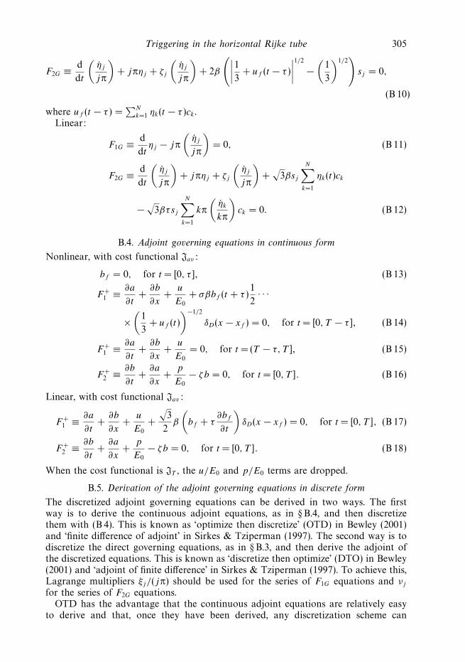
Triggering in the horizontal Rijke tube 305
F2G ≡ d
dt
(ηj
jπ
)+ jπηj + ζj
(ηj
jπ
)+ 2β
(∣∣∣∣13 + uf (t − τ )
∣∣∣∣1/2
−(
1
3
)1/2)
sj = 0,
(B 10)
where uf (t − τ ) =∑N
k=1 ηk(t − τ )ck .Linear:
F1G ≡ d
dtηj − jπ
(ηj
jπ
)= 0, (B 11)
F2G ≡ d
dt
(ηj
jπ
)+ jπηj + ζj
(ηj
jπ
)+
√3βsj
N∑k=1
ηk(t)ck
−√
3βτsj
N∑k=1
kπ
(ηk
kπ
)ck = 0. (B 12)
B.4. Adjoint governing equations in continuous form
Nonlinear, with cost functional Jav:
bf = 0, for t = [0, τ ], (B 13)
F +1 ≡ ∂a
∂t+
∂b
∂x+
u
E0
+ σβbf (t + τ )1
2· · ·
×(
1
3+ uf (t)
)−1/2
δD(x − xf ) = 0, for t = [0, T − τ ], (B 14)
F +1 ≡ ∂a
∂t+
∂b
∂x+
u
E0
= 0, for t =(T − τ, T ], (B 15)
F +2 ≡ ∂b
∂t+
∂a
∂x+
p
E0
− ζb = 0, for t =[0, T ]. (B 16)
Linear, with cost functional Jav:
F +1 ≡ ∂a
∂t+
∂b
∂x+
u
E0
+
√3
2β
(bf + τ
∂bf
∂t
)δD(x − xf ) = 0, for t =[0, T ], (B 17)
F +2 ≡ ∂b
∂t+
∂a
∂x+
p
E0
− ζb = 0, for t =[0, T ]. (B 18)
When the cost functional is JT , the u/E0 and p/E0 terms are dropped.
B.5. Derivation of the adjoint governing equations in discrete form
The discretized adjoint governing equations can be derived in two ways. The firstway is to derive the continuous adjoint equations, as in § B.4, and then discretizethem with (B 4). This is known as ‘optimize then discretize’ (OTD) in Bewley (2001)and ‘finite difference of adjoint’ in Sirkes & Tziperman (1997). The second way is todiscretize the direct governing equations, as in § B.3, and then derive the adjoint ofthe discretized equations. This is known as ‘discretize then optimize’ (DTO) in Bewley(2001) and ‘adjoint of finite difference’ in Sirkes & Tziperman (1997). To achieve this,Lagrange multipliers ξj/(jπ) should be used for the series of F1G equations and νj
for the series of F2G equations.OTD has the advantage that the continuous adjoint equations are relatively easy
to derive and that, once they have been derived, any discretization scheme can
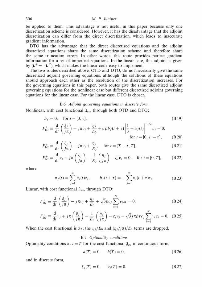
306 M. P. Juniper
be applied to them. This advantage is not useful in this paper because only onediscretization scheme is considered. However, it has the disadvantage that the adjointdiscretization can differ from the direct discretization, which leads to inaccurategradient information.
DTO has the advantage that the direct discretized equations and the adjointdiscretized equations share the same discretization scheme and therefore sharethe same truncation errors. In other words, this route provides perfect gradientinformation for a set of imperfect equations. In the linear case, this adjoint is givenby (L+ = −LH ), which makes the linear code easy to implement.
The two routes described above, OTD and DTO, do not necessarily give the samediscretized adjoint governing equations, although the solutions of these equationsshould approach each other as the resolution of the discretization increases. Forthe governing equations in this paper, both routes give the same discretized adjointgoverning equations for the nonlinear case but different discretized adjoint governingequations for the linear case. For the linear case, DTO is chosen.
B.6. Adjoint governing equations in discrete form
Nonlinear, with cost functional Jav , through both OTD and DTO:
bf = 0, for t =[0, τ ], (B 19)
F +1G ≡ d
dt
(ξj
jπ
)− jπνj +
ηj
E0
+ σβbf (t + τ )
∣∣∣∣13 + uf (t)
∣∣∣∣−1/2
cj = 0,
for t = [0, T − τ ], (B 20)
F +1G ≡ d
dt
(ξj
jπ
)− jπνj +
ηj
E0
, for t = (T − τ, T ], (B 21)
F +2G ≡ d
dtνj + jπ
(ξj
jπ
)− 1
E0
(ηj
jπ
)− ζjνj = 0, for t =[0, T ], (B 22)
where
uf (t) =
∞∑j=1
ηj (t)cj , bf (t + τ ) = −∞∑
j=1
νj (t + τ )sj . (B 23)
Linear, with cost functional Jav , through DTO:
F +1G ≡ d
dt
(ξj
jπ
)− jπνj +
ηj
E0
+√
3βcj
N∑k=1
νksk = 0, (B 24)
F +2G ≡ d
dtνj + jπ
(ξj
jπ
)− 1
E0
(ηj
jπ
)− ζjνj −
√3jπβτcj
N∑k=1
νksk = 0. (B 25)
When the cost functional is JT , the ηj/E0 and (ηj /jπ)/E0 terms are dropped.
B.7. Optimality conditions
Optimality conditions at t = T for the cost functional Jav in continuous form,
a(T ) = 0, b(T ) = 0, (B 26)
and in discrete form,
ξj (T ) = 0, νj (T ) = 0. (B 27)

Triggering in the horizontal Rijke tube 307
Optimality conditions at t = T for the cost functional JT in continuous form,
a(T ) =2T
E0
u(T ), b(T ) =2T
E0
p(T ), (B 28)
and in discrete form,
ξj (T )/(jπ) =2T
E0
ηj (T ), νj (T ) =2T
E0
ηj (T )/(jπ). (B 29)
These apply to both the linear and the nonlinear governing equations.
B.8. Gradient information
Gradient information at t = 0 for the cost functional Jav in continuous form,
∂L
∂u0
=a(0)
T− Eav
E20
u0,∂L
∂p0
=b(0)
T− Eav
E20
p0, (B 30)
and in discrete form,
∂L
∂η0j
=1
T
(ξj (0)
jπ
)− Eav
E20
η0j,
∂L
∂(η0j/jπ)
=νj (0)
T− Eav
E20
(η0j
jπ
). (B 31)
Gradient information at t = 0 for the cost functional JT in continuous form,
∂L
∂u0
=a(0)
T− 2
ET
E20
u0,∂L
∂p0
=b(0)
T− 2
ET
E20
p0, (B 32)
and in discrete form,
∂L
∂η0j
=1
T
(ξj (0)
jπ
)− 2
ET
E20
η0j,
∂L
∂(η0j/jπ)
=νj (0)
T− 2
ET
E20
(η0j
jπ
). (B 33)
These apply to both the linear and the nonlinear governing equations.
REFERENCES
Ananthkrishnan, N., Deo, S. & Culick, F. 2005 Reduced-order modeling and dynamics ofnonlinear acoustic waves in a combustion chamber. Combust. Sci. Technol. 177, 221–247.
Ashwin, P. & Timme, M. 2005 Unstable attractors: existence and robustness in networks of oscillatorswith delayed pulse coupling. Nonlinearity 18 (5), 2035–2060.
Balasubramanian, K. & Sujith, R. I. 2008a Thermoacoustic instability in a Rijke tube: non-normality and nonlinearity. Phys. Fluids 20, 044103.
Balasubramanian, K. & Sujith, R. I. 2008b Non-normality and nonlinearity in combustion–acoustic interaction in diffusion flames. J. Fluid Mech. 594, 29–57.
Bewley, T. 2001 Flow control: new challenges for a new Renaissance. Prog. Aerosp. Sci. 37, 21–58.
Butler, K. M. & Farrell, B. F. 1992 Three-dimensional optimal perturbations in viscous shearflow. Phys. Fluids A 4 (8), 1637–1650.
Dowling, A. P. 1997 Nonlinear self-excited oscillations of a ducted flame. J. Fluid Mech. 346,271–290.
Dowling, A. P. 1999 A kinematic model of a ducted flame. J. Fluid Mech. 394, 51–72.
Duguet, Y., Willis, A. P. & Kerswell, R. R. 2008 Transition in pipe flow: the saddle structure onthe boundary of turbulence. J. Fluid Mech. 613, 255–274.
Engelborghs, K., Luzyanina, T. & Roose, D. 2002 Numerical bifurcation analysis of delaydifferential equations using DDE-BIFTOOL. ACM Trans. Math. Softw. 28 (1), 1–21.
Heckl, M. 1990 Nonlinear acoustic effects in the Rijke tube. Acustica 72, 63.
Henningson, D. S. & Reddy, S. C. 1994 On the role of linear mechanisms in transition to turbulence.Phys. Fluids 6 (3), 1396–1398.
308 M. P. Juniper
Jahnke, C. C. & Culick, F. E. C. 1994 Application of dynamical systems theory to nonlinearcombustion instabilities. J. Propul. Power 10, 508–517.
Juniper, M. P. 2010 Transient growth in the horizontal Rijke tube: nonlinear optimal initial states.In N3L International Workshop T.U.M. Munich, Germany.
Juniper, M. P. & Waugh, I. C. 2010 Bypass transition to sustained thermoacoustic oscillations ina linearly stable Rijke tube. In 16th AIAA/CEAS Aeroacoustics Conference, KTH, Stockholm,Sweden. AIAA.
Landau, L. D. & Lifshitz, E. M. 1959 Fluid Mechanics . Pergamon.
Lieuwen, T. 2002 Experimental investigation of limit-cycle oscillations in an unstable gas turbinecombustor. J. Propul. Power 18 (1), 61–67.
Matveev, I. 2003 Thermo-acoustic instabilities in the Rijke tube: experiments and modeling. PhDthesis, CalTech, Pasadena, CA.
Nagaraja, S., Kedia, K. & Sujith, R. I. 2009 Characterizing energy growth during combustioninstabilities: singular values or eigenvalues? Proc. Combust. Inst. 32, 2933–2940.
Nicoud, F., Benoit, L., Sensiau, C. & Poinsot, T. 2007 Acoustic modes in combustors with compleximpedances and multidimensional active flames. AIAA J. 45 (2), 426–441.
Noiray, N., Durox, D., Schuller, T. & Candel, S. M. 2008 A unified framework for nonlinearcombustion instability analysis based on the flame describing function. J. Fluid Mech. 615,139–167.
Press, H. P., Teukolsky, S. A., Vetterling, W. T. & Flannery, B. P. 1992 Numerical Recipes inFortran 77. Cambridge University Press.
Reddy, S. C. & Henningson, D. S. 1993 Energy growth in viscous channel flows. J. Fluid Mech.252, 209–238.
Schmid, P. J. 2007 Nonmodal stability theory. Annu. Rev. Fluid Mech. 39, 129–162.
Schmid, P. J. & Henningson, D. S. 2001 Stability and Transition in Shear Flows. Springer.
Schneider, T. M., Eckhardt, B. & Yorke, J. A. 2007 Turbulence transition and the edge of chaosin pipe flow. Phys. Rev. Lett. 99, 034502.
Selimefendigila, F., Sujith, R. I. & Polifke, W. 2010 Identification of heat transfer dynamicsfor non-modal analysis of thermoacoustic stability. Appl. Maths Comput. (in press).doi:10.1016/j.amc.2010.07.051.
Sirkes, Z. & Tziperman, E. 1997 Finite difference of adjoint or adjoint of finite difference? Mon.Weather Rev. 125, 3373–3378.
Skufca, J. D., Yorke, J. A. & Eckhardt, B. 2006 Edge of chaos in a parallel shear flow. Phys.Rev. Lett. 96, 174101.
Strogatz, S. H. 2001 Nonlinear Dynamics and Chaos. Westview Press.
Subramanian, P., Mariappan, S., Sujith, R. I. & Wahi, P. 2010 Application of numericalcontinuation to bifurcation analysis of Rijke tube. In N3L International Workshop T.U.M.Munich, Germany.
Trefethen, L. N., Trefethen, A. E., Reddy, S. C. & Driscoll, T. A. 1993 Hydrodynamic stabilitywithout eigenvalues. Science 261, 578–584.
Waugh, I. C. & Juniper, M. P. 2010 Triggering, bypass transition and the effect ofnoise on a linearly stable thermoacoustic system. Proc. Combust. Inst. 33 (in press).doi:10.1016/j.proci.2010.06.018.
Zinn, B. T. & Lieuwen, T. C. 2005 Combustion instability: basic concepts. In Combustion Instabilitiesin Gas Turbine Engines (ed. T. C. Lieuwen & V. Yang). AIAA.