a unified framework for probabilistic component …deb-basu/slides/cs6240presentation.pdfdebabrota...

Debabrota Basu

A Unified Framework for Probabilistic Component analysis

Debabrota Basu

School of ComputingNational University of Singapore

3 March 2015 Unifying Probabilistic Component Analysis 1

Debabrota Basu

Nicolaou, Mihalis A., Stefanos Zafeiriou, and Maja Pantic. "A unified frameworkfor probabilistic component analysis." Machine Learning and KnowledgeDiscovery in Databases. Springer Berlin Heidelberg, 2014. 469-484.

Reference Paper


Debabrota Basu

Introduction

Overview of CA techniquesPrincipal Component Analysis (PCA)

Linear Discriminant Analysis (LDA)

Locality Preserving Projections (LPP)

Slow Feature Analysis (SFA)

Steps to Unification

Unified Maximum Likelihood frameworkDefining priors and Markov random fields

Maximum likelihood solution

Unified Expectation Minimization frameworkGeneralizing the prior

Expectation step

Minimization step

Experiments

Discussions

Roadmap


Debabrota Basu

Introduction

Roadmap


Debabrota Basu

Component analysis is a method of projecting data to subspace

Subspace is a “manifold” (surface) embedded in a higher dimensional vector space

Data (e.g. images) are represented as points in a high dimensional vector space

Constraints in the natural world and the extraction process causes the points to “live” in a lower dimensional subspace

Dimensionality reductionAchieved by extracting ‘important’ features from the dataset Learning

Desirable to avoid the “curse of dimensionality” in pattern recognition Classification

Examples- PCA, LDA, ICA, LPP, SFA, Kernel methods….

What is Component Analysis?


Debabrota Basu

Projection to Subspaces


• Selection of W– Orthonormal bases

• Y is simply projection of X onto W: Y = WT X

– General independent bases• If N=F, Q is obtained by solving linear system

• If N<F, have to do some optimization (e.g., least squares)

• Different criterion for selecting W leads to different subspace methods

-Motivation for unification

XFxT WFxN YNxT

≈

xi ≈ b=1..Nwbi yb

Sample data set

or

observation space

Projection

matrix

Component set

or

latent space

Debabrota Basu

Overview of CA techniquesPrincipal Component Analysis (PCA)

Linear Discriminant Analysis (LDA)

Locality Preserving Projections (LPP)

Slow Feature Analysis (SFA)

Roadmap


Debabrota Basu

Principal Component Analysis


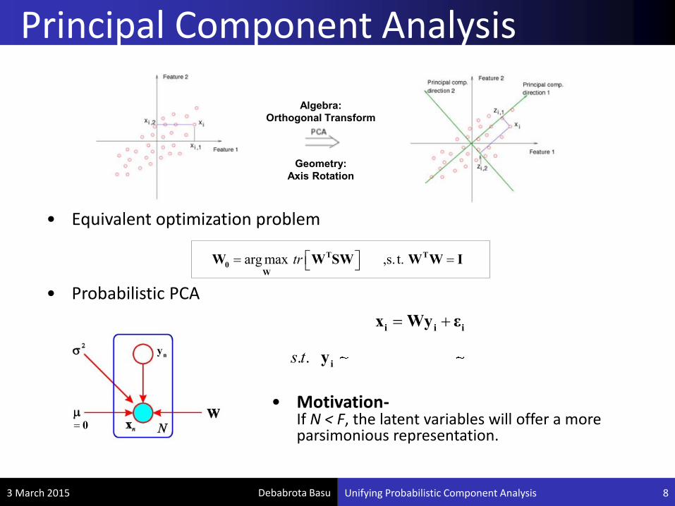
• Motivation-If N < F, the latent variables will offer a more parsimonious representation.

Algebra:

Orthogonal Transform

Geometry:

Axis Rotation

arg max ,s. t.tr T T

0W

W W SW W W I

ny

0

i i ix Wy ε

2. . ( ) , xs t i iy 0,I ε 0 I

• Equivalent optimization problem

• Probabilistic PCA

Debabrota Basu

Linear Discriminant Analysis

14 August 2015

Unifying Probabilistic Component Analysis 9

• Motivation-Minimizing within-class variance i.e, and maximizing between-class variance i.e,

• This is equivalent to finding a projection

• This can be adopted as

1 2s s

2

1 2m m

0 arg max b

w

T

TW

W S WW

W S W

0 arg min [ ] , . .w btr s t T T

W

W W S W W S W I

• Probabilistic LDA is given as a generative model

( ) ( )P Ty m,AΨA

( | ) ( )P Tx y m,AA

• Achilles’ heel of PLDA:

Every class has to have samenumber of data points.

-Unrealistic!!!

Debabrota Basu

Locality Preserving Projections


• Motivation-Finding a projection W such that locality of original samples is preserved in latent space.

• This is equivalent to

• Here, U represents the Heat kernel. This is used to represent locality.

• results a heavy penalty if the data points are mapped far apart.

• No probabilistic version was proposed.

L = D-U

0 arg min [ ] , . .tr s t T T T T

W

W W XLX W W XDX W I

( )diagD U1

2

[ ] expi j

ij

x xu

U

𝑤𝑖𝑗

Debabrota Basu

Slow Feature Analysis


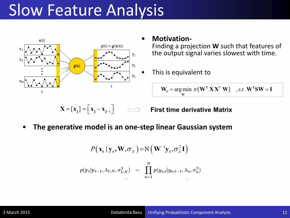
• Motivation-Finding a projection W such that features of the output signal varies slowest with time.

• This is equivalent to

0 arg min [ ] , . .Ttr s t ..

T T

W

W W XX W W SW I

1[ ]

. .

j j jX x x x First time derivative Matrix

• The generative model is an one-step linear Gaussian system

1 2, ,X XP t t tx | y ,W W y I

Debabrota Basu


Roadmap


Debabrota Basu

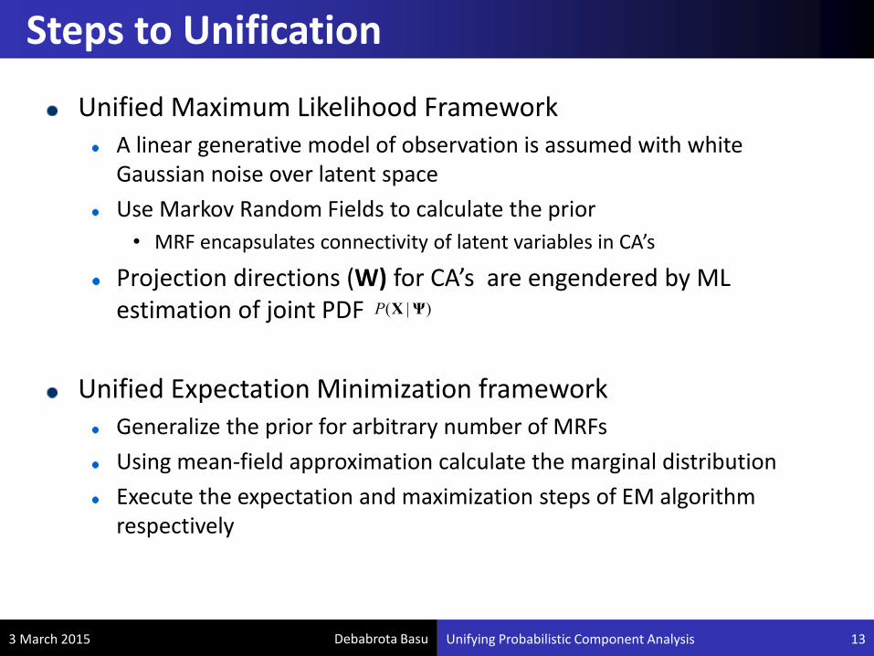
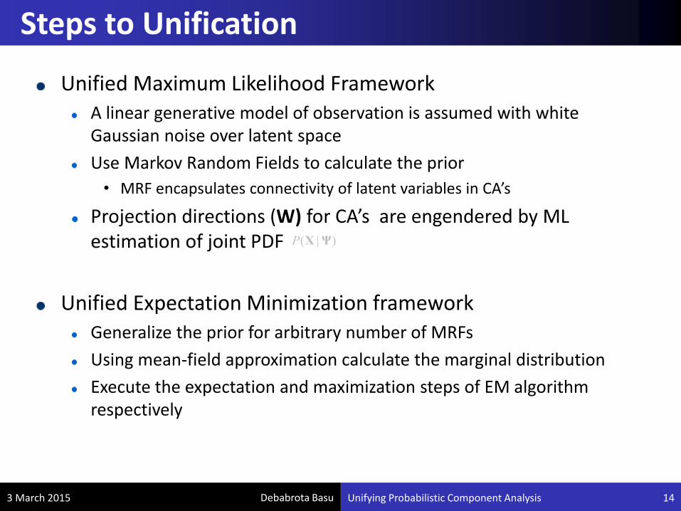
Unified Maximum Likelihood FrameworkA linear generative model of observation is assumed with white Gaussian noise over latent space

Use Markov Random Fields to calculate the prior

• MRF encapsulates connectivity of latent variables in CA’s

Projection directions (W) for CA’s are engendered by ML estimation of joint PDF



( | )P X Ψ

Debabrota Basu

Unified Expectation Minimization frameworkGeneralize the prior for arbitrary number of MRFs

Using mean-field approximation calculate the marginal distribution

Execute the expectation and maximization steps of EM algorithm respectively



( | )P X Ψ

Debabrota Basu

Unified Maximum Likelihood frameworkCalculation of priors

Maximum likelihood solution

Roadmap


Debabrota Basu

MRFs and Latent Connectivity


Fully Connected MRF Within-class Connected MRF Locally Connected MRF

EM-LDAEM-PCA EM-LPP

Debabrota Basu

The unified formula for the prior of component analysis methods is of the form

and are functional form of potentials which encapsulate the latent covariance connectivity of neighborhoods.

and are functions of parameters of MRF

Calculation of priors


1

( ) exp2

P tr tr

(1) (1) T (2) (2) TY | Λ YB Y Λ YB Y

(1)B

(2)B

PCA LDA LPP SFA

(1)B

(2)B

I

1

T T

M 11

c diag cM I C

t M I M

-1L D L

T

1 1 1K = P P

D I I

(1)Λ

(2)Λ 2

1: 1:,N N

Debabrota Basu

If we consider the linear generative model,

Thus, the likelihood will be

Maximum likelihood solution for our model gives

W simultaneously diagonalises and

Maximum Likelihood (ML) solution


1 2, . . , xs t i i i ix W y ε ε 0 I

2 1 2, ,x t xP t tx | y ,W W y

2

1

, |T

x

t

P P P d

t tX |Ψ x | y ,W Y Y

2 2 (1) (1) T T ( ) ( ) T TI Λ WXB X W Λ WXB X W

𝐗𝐁 𝟏 𝐗𝐓 𝐗𝐁 𝟐 𝐗𝐓.

Debabrota Basu

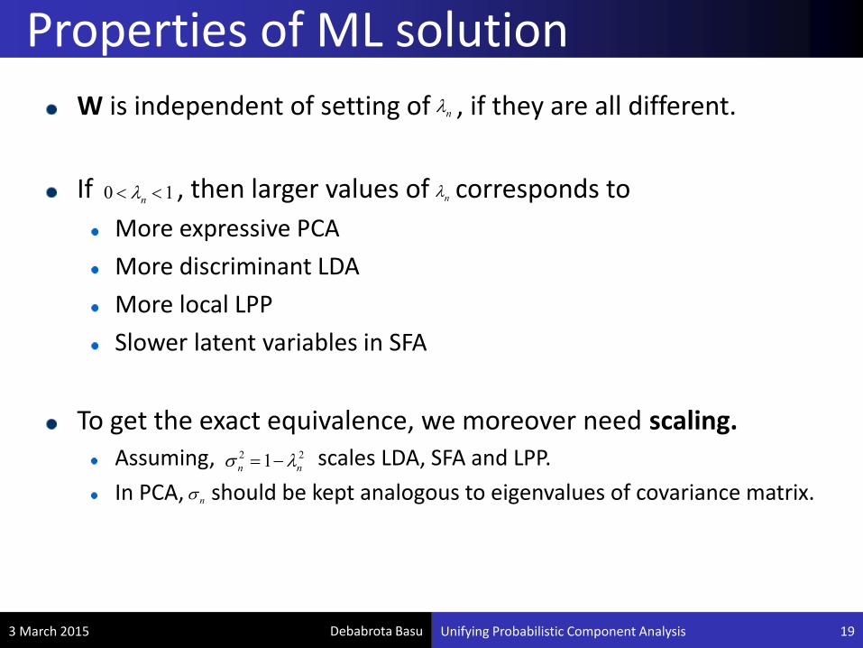
W is independent of setting of , if they are all different.

If , then larger values of corresponds to

More expressive PCA

More discriminant LDA

More local LPP

Slower latent variables in SFA

To get the exact equivalence, we moreover need scaling.Assuming, scales LDA, SFA and LPP.

In PCA, should be kept analogous to eigenvalues of covariance matrix.

Properties of ML solution


n

0 1n n

2 21n n

n

Debabrota Basu

Unified Expectation Minimization frameworkGeneralizing the prior

Expectation step

Minimization step

Roadmap


Debabrota Basu

Iterative method for parameter ( ) estimation where you have missing data ( ).

Expectation-Maximization


Starting from an initial guess, each iteration consists

An Expectation (E) step

where it computes expectation of log likelihood over pre estimated parameters and available data

A Maximization (M) step

where parameters are updated

Y

( ) log |Q E P i i

Yθ,θ X,Y | θ X,θ

arg max ( )Qi+1 i

θ

θ θ,θ

Debabrota Basu

The prior is defined as product of MRFs as

If the linear generative model is assumed, using mean-field approximation we can write

depends on model specific connectivity and depends on

depends on

Linear generative model is assumed.

Generalizing prior


1

,T

i

i

mM M

imM [ ] iy

𝛴𝑀 2

1: 1:,N N

Debabrota Basu

Compute the first order moment on the latent posterior which returns a Gaussian distribution.

It in turn gives us, expectation terms for missing data

Expectation Step


mean

covariance

Debabrota Basu

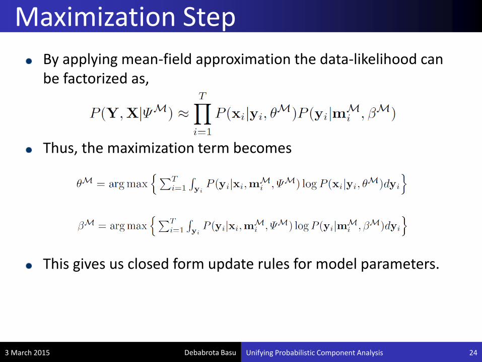
By applying mean-field approximation the data-likelihood can be factorized as,

Thus, the maximization term becomes

This gives us closed form update rules for model parameters.

Maximization Step


Debabrota Basu

EM-PCAEquivalent to PPCA when

Generally shifted by a mean field

Models per dimension variance, that PCA cannot

Complexity is , unlike for deterministic PCA (F,N<<T)

EM for SFAUndirected MRF interpretation• Autoregressive SFA

• Can learn bi-directional latent dependencies

Directed Dynamic Bayesian Network interpretation• A direction specific model of our EM model with directed MRF prior

Probabilistic LDAOnly need to estimate likelihood of each test datum in each class

Probabilistic nature can be exploited to infer the most likely class assignment of unseen data

Features of EM solutions


0 1n nand

( )O TNF 3( )O T

Debabrota Basu

Experiments

Roadmap


Debabrota Basu

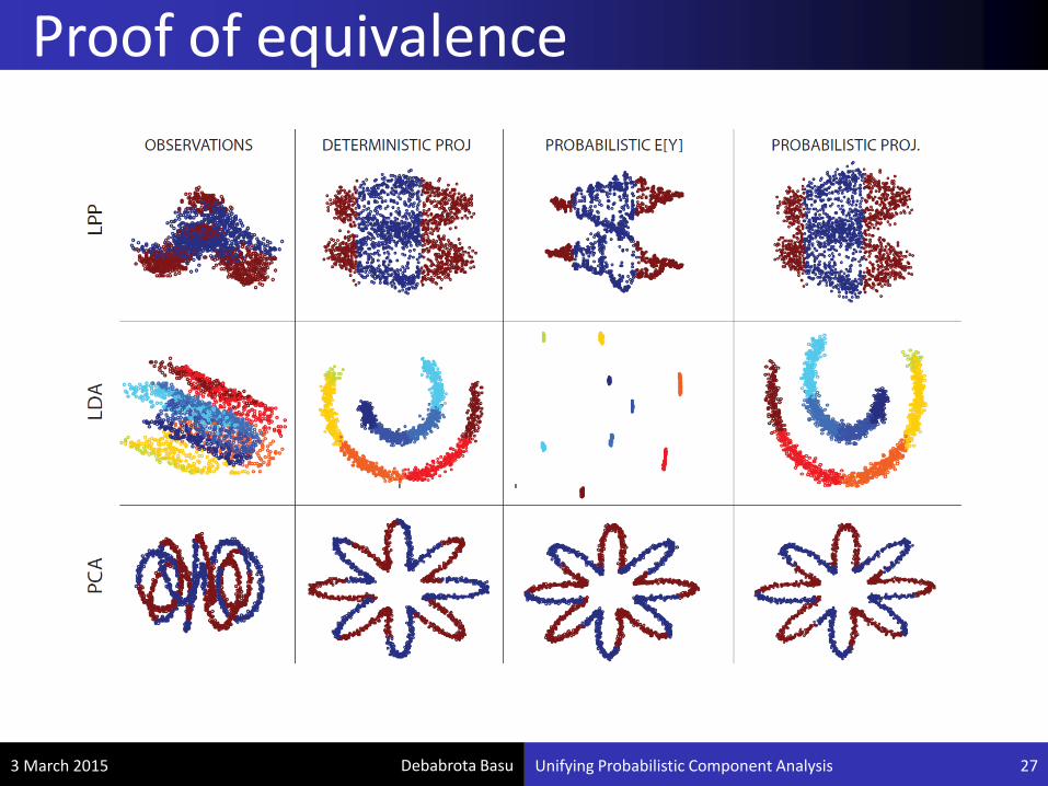
Proof of equivalence


Debabrota Basu

Face recognition: EM-LDA


Debabrota Basu

Face Visualization: EM-LPP


Debabrota Basu

Discussions

Roadmap


Debabrota Basu

All component analysis methods are constraint based subspace projection

Subspace methods can be modeled probabilisticallyBy defining a prior as product of MRFs having different latent neighborhood connectivity

Estimating maximum likelihood depending on a linear model with white Gaussian noise

An EM algorithm for each of the subspace method can be proposed

Use of mean field approximation and MRF priors give us the updates

Discussions(1)


Debabrota Basu

EM variants of these algorithms are compatible with state-of-art

Most variants are less computationally complex

This method models variance per dimension

Efficient CA’s can be generated just by varying prior MRF connectivity

Experiments show the EM variants are more immune to noise in data and also more efficient

Discussions(2)


Debabrota Basu

Questions?


Debabrota Basu

Thank you…


a unified framework for probabilistic component …deb-basu/slides/cs6240presentation.pdfdebabrota...

Documents