DISCUSSION PAPER SERIES

ABCD

No. 10783

INNOVATION, EMISSIONS POLICY, AND COMPETITIVE ADVANTAGE IN THE DIFFUSION OF EUROPEAN DIESEL

AUTOMOBILES

Eugenio J. Miravete, Maria J. Moral and Jeff Thurk

INDUSTRIAL ORGANIZATION

ISSN 0265-8003

INNOVATION, EMISSIONS POLICY, AND COMPETITIVE ADVANTAGE IN THE DIFFUSION OF EUROPEAN DIESEL AUTOMOBILES

Eugenio J. Miravete, Maria J. Moral and Jeff Thurk

Discussion Paper No. 10783

August 2015 Submitted 14 August 2015

Centre for Economic Policy Research 77 Bastwick Street, London EC1V 3PZ, UK

Tel: (44 20) 7183 8801 www.cepr.org

This Discussion Paper is issued under the auspices of the Centre’s research programme in INDUSTRIAL ORGANIZATION. Any opinions expressed here are those of the author(s) and not those of the Centre for Economic Policy Research. Research disseminated by CEPR may include views on policy, but the Centre itself takes no institutional policy positions.

The Centre for Economic Policy Research was established in 1983 as an educational charity, to promote independent analysis and public discussion of open economies and the relations among them. It is pluralist and non‐partisan, bringing economic research to bear on the analysis of medium‐ and long‐run policy questions.

These Discussion Papers often represent preliminary or incomplete work, circulated to encourage discussion and comment. Citation and use of such a paper should take account of its provisional character.

Copyright: Eugenio J. Miravete, Maria J. Moral and Jeff Thurk

INNOVATION, EMISSIONS POLICY, AND COMPETITIVE ADVANTAGE IN THE DIFFUSION OF

EUROPEAN DIESEL AUTOMOBILES†

Abstract

Spurred by Volkswagen's introduction of the TDI diesel engine in 1989, market penetration of diesel cars in Europe increased from 10% in 1990 to over 50% in 2000. Using Spanish automobile registration data, we estimate an equilibrium discrete choice, oligopoly model of horizontally differentiated products. We find that changing product characteristics and the increasing popularity of diesels leads to correlation between observed and unobserved (to the researcher) product characteristics, an aspect we allow for in the estimation. Despite widespread imitation by its rivals, Volkswagen was able to capture 32% of the potential innovation rents and diesels accounted for approximately 60% of the firm's profits. Moreover, diesels amounted to an important competitive advantage for European auto makers over foreign imports. We provide evidence that the greenhouse emissions policy enacted by European regulators, and not preferential fuel taxes, enabled the adoption of diesels. In so doing, this non‐tariff policy was equivalent to a 20% import tariff; effectively cutting imports in half.

JEL Classification: F13, L62 and O33 Keywords: diesel cars, emission standards, import tariff equivalence and innovation rents

Eugenio J. Miravete miravete@eco.utexas.edu University of Texas at Austin, UEA and CEPR Maria J. Moral mjmoral@cee.uned.es Universidad Nacional de Educacion a Distancia and GRiEE Jeff Thurk jthurk@nd.edu University of Notre Dame

† This paper supersedes “Protecting the European Automobile Industry through Environmental Regulation: The Adoption of Diesel Engines." We thank Allan Collard-Wexler, Kenneth Hendricks, Tom Holmes, Cristian Huse, Jeff Prince, and audiences at several seminars and conferences. We are solely responsible for any errors that may still remain. Moral gratefully acknowledges funding from the Spanish Ministry of Education and Science through grant ECO2010-18947.

1 Introduction

The European automobile market is inconspicuously unique in a way that might escape tourists

traveling to the Old Continent. Most American tourists will recognize that European vehicles are

smaller (something not unique to Europe) but those renting a vehicle will likely be surprised to learn

that they have to refuel with diesel rather than gasoline. The introduction of a new technology – the

turbocharged direct injection (tdi) diesel engine – by volkswagen in 1989 took diesel penetration

from around 10% market share in most European countries to in excess of 60% market share by

the beginning of the financial crisis in 2008.1 Surprisingly, this dramatic transformation of the

European automobile industry has failed to attract the interest of innovation economists.2

We evaluate the effects of this technological innovation using automobile registration data

from Spain – a country which exhibited diesel adoption rates representative of Europe as a whole.

We employ the equilibrium discrete choice oligopoly model of Berry, Levinsohn and Pakes (1995),

henceforth BLP, to study an industry which is far from competitive and where products are

horizontally differentiated. The BLP framework has become a workhorse model in the empirical

Industrial Organization literature as it is flexible enough to generate plausible substitution patterns

between similar products while accounting for product characteristics known to consumers and firms

but not to the researcher. For us, the framework also provides an opportunity to evaluate many

counterfactuals of interest since changes in regulation, taxes, or demand and supply conditions

result in new equilibrium prices and market configurations.

An important identification assumption used in the standard BLP estimation is that observ-

able and unobservable product characteristics are uncorrelated. This is problematic in our context

as we observe both a substantial increase in diesel purchases and changing product characteristics.

Further, both observable and unobservable product attributes determine sales of vehicles but the

latter likely drive the sales of diesels as consumers discover the greater performance of this new

technology during the diffusion period of our sample. Instead, our estimation approach accounts

for the potential correlation between observable and unobservable automobile characteristics by

allowing firms to choose product attributes, observed or otherwise. Firm product choices then

influence optimal equilibrium prices of automobile manufacturers through own and cross-price

effects of manufacturers’ vehicle offerings.

1 See Automobile Registration and Market Share of Diesel Vehicles in “ACEA European Union Economic Report,”December 2009. This quick adoption process compares favorably to many others innovations such as steam anddiesel locomotives (Greenwood, 1997); the basic oxygen furnaces for steel mills (Oster, 1982); and the coal-fired,steam-electric high-pressure power generation (Rose and Joskow, 1990).

2 Perhaps a plausible explanation for this state of affairs is that well over two decades after the tdi breakthroughthe European automobile market remains an oddity in the global automobile industry as diesel passenger vehiclesfailed to succeed anywhere else except, recently, in India. See Chug, Cropper and Narain (2011).

– 1 –

We are not the first to allow for correlation between observed and unobserved product

characteristics. Indeed, Petrin and Seo (2015) first made use of optimal instruments to account for

the possibility of endogenous product characteristics. We borrow their methodology and confirm

most of their conclusions obtained using the original BLP database. We find significant correlation

between observed and the estimated unobserved product characteristics. We also find that our

estimation approach yields demand estimates which are more elastic than employing a standard

BLP estimation and more significant point estimates, particularly for the random coefficients – a

noted difficulty with the standard BLP model. The cost of obtaining more efficient estimates of

random coefficients is the substantially increased computational burden but our results add to the

claim of Petrin and Seo (2015) that BLP overestimates equilibrium markups.

In order to measure the importance of the tdi innovation we follow an approach similar

to Berry, Levinsohn and Pakes (1999) in addressing the effects of Voluntary Export Restraints, or

Petrin (2002) to account for the redistribution of profits among auto makers after the introduction

of the minivan. We find that eliminating diesels altogether generates significant losses for European

auto makers – the firms who adopted the technology – but would have resulted in nearly a doubling

in market share for non-European auto makers, particularly Asian manufacturers such as Honda

and Toyota. This indicates that diesel vehicles represented a significant competitive advantage

for domestic (i.e., European) auto makers. We also show that despite large-scale imitation by its

European rivals, volkswagen was able to secure significant profits from the tdi and captured

32% of the potential rents from its innovation.

Subsidization of diesel fuel is commonly credited with providing drivers with strong in-

centives to purchase diesel vehicles. We evaluate this hypothesis and conclude that diesel fuel

subsidization is only responsible for a small 1.5% additional market share of diesel vehicles in 2000.

This is clearly not enough to explain the large shift of demand in favor of diesel vehicles.3

Instead we provide evidence that the success of diesel vehicles in Europe was, in large

part, the consequence of the European greenhouse standards implemented in the early 1990s. If

European authorities had followed an emissions policy similar to the United States, focused on

the effects of acid rain, the overwhelming adoption of diesels automobiles would have not taken

place in Europe, leaving diesels as a market niche well below the levels of the 1980s. Under such

alternative policy, mileage conscious drivers would have shifted their purchases towards the fuel

efficient gasoline Asian imports, leading to a near doubling of their market share from 11% to 19

percent.

3 Linn (2014) relates fuel taxes and environmental considerations to explain the within-Europe, cross-country differ-ences in diesel automobiles market penetration while Grigolon, Reynaert and Verboven (2014) evaluate whether afuel tax or a tax linked to vehicle fuel efficiency helps achieve larger fuel savings by steering consumers to purchasedifferent cars and/or driving less. Both studies use a more mature market sample period than ours, 2002-2010 and1998-2011, respectively, once the growth of diesel penetration rates have stabilized.

– 2 –

Therefore, the European emissions policy induces important distortion effects in the Euro-

pean automobile market. We find that the induced protection was substantial, nearly the equivalent

of a 20% import tariff when the actual import duty amounted only to 10.3%. These results are

important as they provide evidence that in a world with ever more free trade agreements, national

policies such as environmental regulations might be used as a tool to favor local manufacturers over

competitive imports, e.g., Ederington and Minier (2003) – an important finding and perhaps the

most original contribution of the paper.

To be clear, we are not claiming that European regulators designed their emission standards

strategically to explicitly promote domestic auto makers. Rather, we argue that regardless of

whether it was the intent of the policymaker or not, environmental policy became a powerful tool

to protect the domestic European auto makers.4 Linking environmental and trade policies, our

work builds on the literature related to the interaction of domestic policy and international trade.5

Our work contributes to this literature by being, to the best of our knowledge, the first application

of equilibrium models commonly used in empirical industrial organization to provide evidence of

rent-seeking by countries using domestic regulation policy.

The paper is organized as follows. In section 2, we describe the tdi innovation, its imitation

by European auto makers, and summarize the main features of the Spanish market for diesel

automobiles. Section 3 describes the equilibrium model of discrete choice demand for horizontally

differentiated products with endogenous prices and characteristics. Section 4 reports the estimation

results, summarizes the main findings, and documents the need to obtain optimal instrumental

variables to address the potential correlation between observed and unobserved product character-

istics. Section 5 addresses the dissipation of volkswagen’s innovation rents due to the generality

of the tdi technology and the increase of competition in the diesel segment. In Section 6 we

discuss the trade effects of emissions policies enforced by European regulators and investigate the

equilibrium implications different emission standards: survival of diesel engines under the U.S. NOx

emission standards and the magnitude of the implicit trade protection level induced by the European

environmental regulation. In Section 7 we discuss the robustness of our results by evaluating the

role of favorable diesel fuel taxation; comparing our results to those implied by a standard BLP

model and estimation strategy; and addressing alternative modeling assumptions. Finally, Section 8

concludes. Details of the estimation, additional results, data sources, and institutional details of

the Spanish automobile market are documented in the Appendices.

4 As far as we know the trade consequences of the environmental policy did not occur by design, i.e., it was not anexplicit attempt to protect the European automobile industry, but rather the result of legislative inertia.

5 The seminal contribution on this topic is Bhagwati and Ramaswami (1963) who address the substitutability betweendomestic policy and import tariffs. More recent works (e.g., Staiger 1995, Bagwell and Staiger 2001, Deardorff 1996,Thurk 2014) take a more game theoretic approach and show that countries can use their domestic policies to extractrents from the rest-of-the-world leading to a suboptimal aggregate outcome.

– 3 –

2 The European Market for Diesel Automobiles in the 1990s

This section intends to get the reader familiarized with the basic characteristics of the diesel

technology and tdi innovation; the institutional features of the European market that allowed

for a swift take off of diesel sales in the early 1990s; and the evolution of the Spanish market.

2.1 What Is a TDI Engine?

In the late 19th century, Rudolf Diesel designed an internal combustion engine in which heavy fuel

self-ignites after being injected into a cylinder where air has been compressed to a much higher

degree than in gasoline engines. However, it was only in 1927, many years after Diesel’s death, that

the German company Bosch built the injection pump that made the development of the engine for

trucks and automobiles possible. The first diesel vehicles sold commercially followed soon after: the

1933 Citroen Rosalie and the 1936 Mercedes-Benz 260D. Large passenger and commercial diesel

vehicles were common in Europe from the late 1950s through the 1990s.

In 1989, Volkswagen introduced the tdi diesel engine in its Audi 100 model, a substantial

improvement over the existing Perkins technology. A tdi engine uses a fuel injector that sprays fuel

directly into the combustion chamber of each cylinder. The turbocharger increases the amount of air

going into the cylinders and an intercooler lowers the temperature of the air in the turbo, thereby

increasing the amount of fuel that can be injected and burned. Overall, tdi allows for greater

engine performance while providing more torque at low r.p.m. than alternative gasoline engines.

They are also credited with being more durable and reliable than gasoline engines although this

was something yet to be learned by consumers at the time this technology was first introduced.6

Following this major technological breakthrough, Europeans enthusiastically embraced diesel au-

tomobiles. The incredible pace of adoption of diesel automobiles suggests that the tdi proved to

be a significant technological and consumers gained little from waiting for additional incremental

improvements, which have been few and of minor importance.7

2.2 Initial Market Conditions

There are important institutional circumstances that helped build the initial conditions that were

particularly favorable for the adoption of this new technology in Europe. The key element triggering

all these favorable development is the European Fuel Tax Directive of the 1973.

6 See the 2004 report “Why Diesel?” from the European Association of Automobile Manufacturers (ACEA).7 This argument was first put forward by Schumpeter (1950, p.98) and later formalized by Balcer and Lippman

(1984). More recently, it has recently been used by Manuelli and Seshadri (2014) to explain the half a century timespan needed for the diffusion of the much studied case of tractors.

– 4 –

Following the first oil crisis of 1973, the then nine members of the European Economic

Community gathered in Copenhagen in December of that year and agreed to develop a common

energy policy. A main idea was to harmonize fuel taxation across countries so that drivers, and fossil

fuel users in general, faced a single and consistent set of incentives to save energy. Coordination

also limited the possibility of arbitrage across state lines as well as some countries free riding on the

conservation efforts of other members. Fuel prices or their taxation were not harmonized overnight

but the new Tax Directive offered principles of taxation that were eventually followed in every

country. For the purposes of this study, the two most prominent features of this Directive are that

fuels are taxed by volume rather than by their energetic content and that diesel fuel is taxed at a

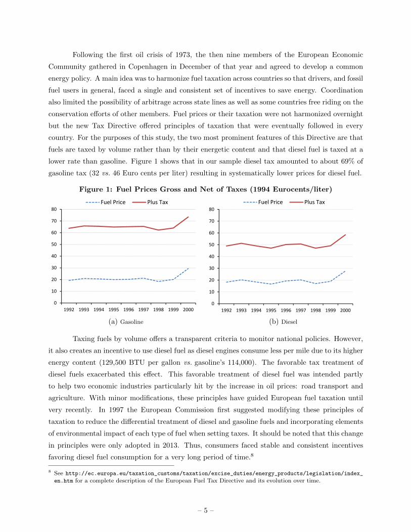
lower rate than gasoline. Figure 1 shows that in our sample diesel tax amounted to about 69% of

gasoline tax (32 vs. 46 Euro cents per liter) resulting in systematically lower prices for diesel fuel.

Figure 1: Fuel Prices Gross and Net of Taxes (1994 Eurocents/liter)

0

10

20

30

40

50

60

70

80

1992 1993 1994 1995 1996 1997 1998 1999 2000

Fuel Price Plus Tax

(a) Gasoline

0

10

20

30

40

50

60

70

80

1992 1993 1994 1995 1996 1997 1998 1999 2000

Fuel Price Plus Tax

(b) Diesel

Taxing fuels by volume offers a transparent criteria to monitor national policies. However,

it also creates an incentive to use diesel fuel as diesel engines consume less per mile due to its higher

energy content (129,500 BTU per gallon vs. gasoline’s 114,000). The favorable tax treatment of

diesel fuels exacerbated this effect. This favorable treatment of diesel fuel was intended partly

to help two economic industries particularly hit by the increase in oil prices: road transport and

agriculture. With minor modifications, these principles have guided European fuel taxation until

very recently. In 1997 the European Commission first suggested modifying these principles of

taxation to reduce the differential treatment of diesel and gasoline fuels and incorporating elements

of environmental impact of each type of fuel when setting taxes. It should be noted that this change

in principles were only adopted in 2013. Thus, consumers faced stable and consistent incentives

favoring diesel fuel consumption for a very long period of time.8

8 See http://ec.europa.eu/taxation_customs/taxation/excise_duties/energy_products/legislation/index_

en.htm for a complete description of the European Fuel Tax Directive and its evolution over time.

– 5 –

This favorable tax treatment of diesel fuel fostered the sale of diesel vehicles from the

mid-1970s on. By the end of the 1980s, some large passenger cars and many commercial vehicles

comprising almost 10% of the market ran on diesel fuel. Thus, when the tdi was first sold in 1989,

Europeans, unlike Americans, were familiar with diesels and did not have a particularly negative

perception of the quality of diesel vehicles.9 More importantly, Europeans did not have to cope with

the additional network costs commonly delaying the adoption of alternative fuels: by 1990 diesel

pumps were ubiquitous, indeed available in every gas station, and it was easy to find mechanics

trained to service these vehicles in case repairs were needed.

Initial conditions were thus more conducive to the success of the tdi technology than in

any other automobile market in the world. And yet, it was not obvious that consumers were going

to end up embracing this new technology when volkswagen introduced the tdi engine the way

they did it. Diesels are known to achieve better mileage than otherwise identical gasoline vehicles,

leading to future fuel cost savings, but they are also more expensive to purchase, presumably due

to higher production costs or because manufacturers’ attempt to capture consumer rents of drivers

favoring diesel vehicles.10 But since the diffusion of tdi coincided with a long period of historically

low and stable fuel prices documented in Figure 1, the value of potential fuel savings were limited

and so was the manufacturers’ ability to overprice diesel automobiles.

2.3 Imitation

Figure 2 demonstrates that imitation of the tdi occurred quickly and was largely driven by rival

European auto makers. This indicates the ineffectiveness of volkswagen to defend its innovation

via the patent system since it was not difficult for rival firms to offer their own equivalent diesel

models in a relatively short period of time. This suggests a low cost of imitation – a trait which

characterizes all “general technologies” (e.g., Bresnahan 2010) – due to the fact the technology can

be easily modified or reverse engineered.

For the consumers, imitation led to the introduction of more variety and better quality of

vehicles to choose from while competition intensified in this market segment, keeping diesel vehicles

affordable, and therefore reinforcing the fast diffusion of this new technology.11 When imitation is

9 See http://www.autosavant.com/2009/08/11/the-cars-that-killed-gm-the-oldsmobile-diesel/ for an ac-count of how badly gm’s retrofitted gasoline engines delivered poor performance when running on diesel fuelin the late 1970s and early 1980s and how such experience conformed the negative views of Americans on dieselvehicles for many years.

10Verboven (2002) studies the price premium paid for diesel vehicles relative to otherwise identical gasoline modeland explains it as business strategy aimed to capture some of the rents of consumers with heterogeneous drivinghabits.

11volkswagen was an important firm but not the leader in the Spanish market: renault was by far the leader inthe gasoline segment and psa, which includes the French brands citroen and peugeot, in diesel. See Figure D.1in the Web Appendix.

– 6 –

Figure 2: Number of Diesel Models Offered

0

10

20

30

40

50

60

70

80

90

100

1992 1994 1996 1998 2000

VW PSA Other EU Foreign

easy and potentially massive, uncertainty about recouping sunk investment costs may hinder the

development of new technologies in the first place. Consequently, the financial repercussions for

firms of working with this general technology, are uncertain. We will address this issue in Section 5

for the case of volkswagen.

2.4 Evolution of Automobile Characteristics in Spain

Our data include yearly car registrations by manufacturer, model, and fuel engine type in Spain

between 1992 and 2000. After removing a few observations, mostly of luxury vehicles with extremely

small market shares, our sample is an unbalanced panel comprising 99.2% of all car registrations in

Spain during the 1990s. Spain was the fifth largest automobile manufacturer in the world during

the 1990s and also the fifth largest European automobile market by sales after Germany, France,

the United Kingdom, and Italy. In our sample automobile sales range from 968,334 to 1,364,687

units sold annually.

Figure 3: Automobile Sales and Models by Year and Fuel Type

0

75000

150000

225000

300000

375000

450000

525000

600000

675000

750000

825000

91 92 93 94 95 96 97 98 99 00

Automobile Sales

Gasoline Diesel

(a) Sales (thousands of vehicles)

0

20

40

60

80

100

120

140

91 92 93 94 95 96 97 98 99 00

Number of Models

Gasoline Diesel

(b) Models Available

– 7 –

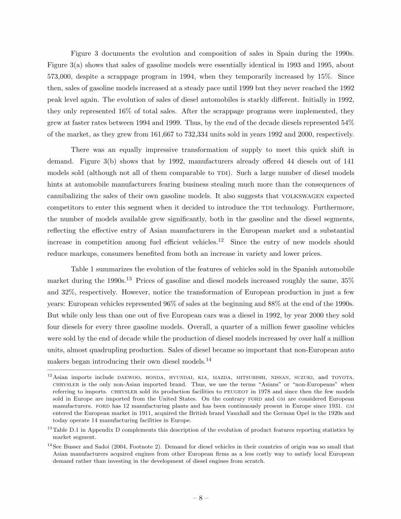
Figure 3 documents the evolution and composition of sales in Spain during the 1990s.

Figure 3(a) shows that sales of gasoline models were essentially identical in 1993 and 1995, about

573,000, despite a scrappage program in 1994, when they temporarily increased by 15%. Since

then, sales of gasoline models increased at a steady pace until 1999 but they never reached the 1992

peak level again. The evolution of sales of diesel automobiles is starkly different. Initially in 1992,

they only represented 16% of total sales. After the scrappage programs were implemented, they

grew at faster rates between 1994 and 1999. Thus, by the end of the decade diesels represented 54%

of the market, as they grew from 161,667 to 732,334 units sold in years 1992 and 2000, respectively.

There was an equally impressive transformation of supply to meet this quick shift in

demand. Figure 3(b) shows that by 1992, manufacturers already offered 44 diesels out of 141

models sold (although not all of them comparable to tdi). Such a large number of diesel models

hints at automobile manufacturers fearing business stealing much more than the consequences of

cannibalizing the sales of their own gasoline models. It also suggests that volkswagen expected

competitors to enter this segment when it decided to introduce the tdi technology. Furthermore,

the number of models available grew significantly, both in the gasoline and the diesel segments,

reflecting the effective entry of Asian manufacturers in the European market and a substantial

increase in competition among fuel efficient vehicles.12 Since the entry of new models should

reduce markups, consumers benefited from both an increase in variety and lower prices.

Table 1 summarizes the evolution of the features of vehicles sold in the Spanish automobile

market during the 1990s.13 Prices of gasoline and diesel models increased roughly the same, 35%

and 32%, respectively. However, notice the transformation of European production in just a few

years: European vehicles represented 96% of sales at the beginning and 88% at the end of the 1990s.

But while only less than one out of five European cars was a diesel in 1992, by year 2000 they sold

four diesels for every three gasoline models. Overall, a quarter of a million fewer gasoline vehicles

were sold by the end of decade while the production of diesel models increased by over half a million

units, almost quadrupling production. Sales of diesel became so important that non-European auto

makers began introducing their own diesel models.14

12Asian imports include daewoo, honda, hyundai, kia, mazda, mitsubishi, nissan, suzuki, and toyota.chrysler is the only non-Asian imported brand. Thus, we use the terms “Asians” or “non-Europeans” whenreferring to imports. chrysler sold its production facilities to peugeot in 1978 and since then the few modelssold in Europe are imported from the United States. On the contrary ford and gm are considered Europeanmanufacturers. ford has 12 manufacturing plants and has been continuously present in Europe since 1931. gmentered the European market in 1911, acquired the British brand Vauxhall and the German Opel in the 1920s andtoday operate 14 manufacturing facilities in Europe.

13Table D.1 in Appendix D complements this description of the evolution of product features reporting statistics bymarket segment.

14See Busser and Sadoi (2004, Footnote 2). Demand for diesel vehicles in their countries of origin was so small thatAsian manufacturers acquired engines from other European firms as a less costly way to satisfy local Europeandemand rather than investing in the development of diesel engines from scratch.

– 8 –

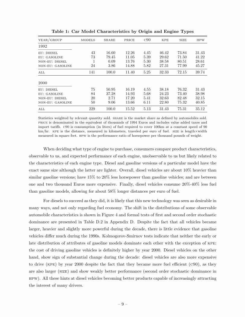
Table 1: Car Model Characteristics by Origin and Engine Types

year/group models share price c90 kpe size hpw

1992

eu: diesel 43 16.60 12.26 4.45 46.42 73.84 31.43eu: gasoline 73 79.45 11.05 5.39 29.62 71.50 41.22non-eu: diesel 1 0.09 13.76 5.30 38.58 80.51 28.61non-eu: gasoline 24 3.86 14.88 5.82 27.31 77.99 45.27

all 141 100.0 11.40 5.25 32.33 72.15 39.74

2000

eu: diesel 75 50.95 16.19 4.55 38.18 76.32 31.43eu: gasoline 84 37.28 14.93 5.68 24.23 73.40 38.98non-eu: diesel 20 2.71 17.20 5.41 32.63 82.48 32.15non-eu: gasoline 50 9.06 13.66 6.11 22.80 75.32 40.85

all 229 100.0 15.52 5.13 31.43 75.31 35.12

Statistics weighted by relevant quantity sold. share is the market share as defined by automobiles sold.price is denominated in the equivalent of thousands of 1994 Euros and includes value added taxes andimport tariffs. c90 is consumption (in liters) of fuel required to cover 100km at a constant speed of 90km/hr. kpe is the distance, measured in kilometers, traveled per euro of fuel. size is length×widthmeasured in square feet. hpw is the performance ratio of horsepower per thousand pounds of weight.

When deciding what type of engine to purchase, consumers compare product characteristics,

observable to us, and expected performance of each engine, unobservable to us but likely related to

the characteristics of each engine type. Diesel and gasoline versions of a particular model have the

exact same size although the latter are lighter. Overall, diesel vehicles are about 10% heavier than

similar gasoline versions; have 15% to 20% less horsepower than gasoline vehicles; and are between

one and two thousand Euros more expensive. Finally, diesel vehicles consume 20%-40% less fuel

than gasoline models, allowing for about 58% longer distances per euro of fuel.

For diesels to succeed as they did, it is likely that this new technology was seen as desirable in

many ways, and not only regarding fuel economy. The shift in the distributions of some observable

automobile characteristics is shown in Figure 4 and formal tests of first and second order stochastic

dominance are presented in Table D.2 in Appendix D. Despite the fact that all vehicles became

larger, heavier and slightly more powerful during the decade, there is little evidence that gasoline

vehicles differ much during the 1990s. Kolmogorov-Smirnov tests indicate that neither the early or

late distribution of attributes of gasoline models dominate each other with the exception of kpe:

the cost of driving gasoline vehicles is definitely higher by year 2000. Diesel vehicles on the other

hand, show sign of substantial change during the decade: diesel vehicles are also more expensive

to drive (kpe) by year 2000 despite the fact that they became more fuel efficient (c90), as they

are also larger (size) and show weakly better performance (second order stochastic dominance in

hpw). All these hints at diesel vehicles becoming better products capable of increasingly attracting

the interest of many drivers.

– 9 –

Figure 4: Change in the Distribution of Automobile Attributes

(a) Gasoline: Mileage (c90) (b) Diesel: Mileage(c90)

(c) Gasoline: Cost of Driving (kpe) (d) Diesel: Cost of Driving (kpe)

(e) Gasoline: size (f) Diesel: size

(g) Gasoline: Performance (hpw) (h) Diesel: Performance (hpw)

– 10 –

3 An Equilibrium Oligopoly Model of the Automobile Industry with

Correlated Product Characteristics

We follow Petrin and Seo (2015) in extending the well-known BLP equilibrium model of discrete

choice oligopoly with horizontally differentiated products to allow for correlation between observed

and unobserved product characteristics. In this section we first present a standard model of

discrete-choice demand with heterogenous consumers. Then we describe an oligopoly model of

supply in which multi-product firms comprising several brands detailed in Table A.1 choose product

characteristics first (e.g., car size) and then compete in retail price given observed and unobserved

product attributes.

3.1 Demand

Demand can be summarized as follows: consumer i derives an indirect utility from buying vehicle

j at time t that depends on price and characteristics of the car:

uijt = xjtβ∗i − α∗i pjt + ξjt + εijt ,

where i = 1, . . . , It; j = 1, . . . , Jt; t = 1992, ..., 2000 .(1)

This Lancasterian approach makes the payoff of a consumer depend on the set of characteristics of

the vehicle purchased, which includes a vector of n observable vehicle characteristics xjt as well as

others that remain unobservable for the econometrician, ξjt, plus the effect of unobserved tastes of

consumer i for vehicle j, εijt, which is assumed i.i.d. multivariate type I extreme value distributed.

We allow for individual heterogeneity in response to vehicle prices and characteristics by modeling

the distribution of consumer preferences over characteristics and prices as multivariate normal with

a mean that shifts with consumer attributes:15

(α∗i

β∗i

)=

(α

βt

)+ ΠtDit + Σtνit , νit ∼ N(0, In+1) . (2)

Consumer i in period t is characterized by one unobserved and a d vector of observed

demographic attributes, Dit and νit. In our case, we allow the estimate of the slope of demand

to vary with per capita income. Πt is a (n + 1) × d matrix of coefficients that measures the

effect of income on the consumer valuation of automobile characteristics, e.g., average valuation

and price responsiveness. Similarly, Σt measures the covariance in unobserved preferences across

15Random coefficients generates correlations in utilities for the various automobile alternatives that relax the restric-tive substitution patterns generated by the Independence of Irrelevant Alternatives property of the logit model.

– 11 –

characteristics. We decompose the deterministic portion of the consumer’s indirect utility into a

common part shared across consumers, δjt, and an idiosyncratic component, µijt. These mean

utilities of choosing product j and the idiosyncratic deviations around them are given by:

δjt = xjtβ + αpjt + ξjt , (3a)

µijt =(xjt pjt

)×(

ΠtDit + Σtνit

). (3b)

Consumers choose to purchase either one of the Jt vehicles available or j = 0, the outside

option of not buying a new car with zero mean utility, µi0t = 0. We therefore define the set of

individual-specific characteristics leading to the optimal choice of car j as:

Ajt (x·t, p·t, ξ·t; θ) = (Dit, νit, εijt) |uijt ≥ uikt ∀k = 0, 1, . . . , Jt , (4)

with θ summarizing all model parameters. The extreme value distribution of random shocks allows

us to integrate over the distribution of εit to obtain the probability of observing Ajt analytically.

The probability that consumer i purchases automobile model j in period t is:

sijt =exp (δjt + µijt)

1 +∑k∈Jt

exp(δkt + µit). (5)

Integrating over the distributions of observable and unobservable consumer attributes Dit

and νit, denoted by PD(Dt) and Pν(νt), respectively, leads to the model prediction of the market

share for product j at time t:

sjt(xt, pt, ξt; θ) =

∫νt

∫Dt

sijtdPDt(Dt)dPνt(νt) , (6)

with s0t denoting the market share of the outside option.

3.2 Supply

The industry is characterized by multi-product automobile manufacturers behaving as oligopolistic,

non-cooperative profit maximizers which take product entry, including engine type, as given and

choose observed and unobserved (to the econometrician) product characteristics and price. While

a firm’s choice of observable product characteristics may be intuitive, it is worthwhile to provide

some intuition as to what it means for a firm to choose an unobservable product characteristic.

For example, increasing popularity of diesel vehicles over the decade may encourage audi to not

only introduce more varieties of diesel vehicles but also improve these vehicles torque, reliability,

– 12 –

et cetera. Ignoring this relationship could potentially lead to a violation of product characteristic

exogeneity, leading to biased results.16

As Petrin and Seo (2015) did with the BLP data, we also consider the problem of a multi-

product firm f which chooses product characteristics xkj in period t to solve:

maxxkj

E

∑r∈Ff

(pr − cr)× sr(·)∣∣∣Ψf

, (7)

where Ff is the set of vehicles of all brands sold by firm f and Ψf is its information set. The t

subscript has been dropped to simplify notation. The subsequent optimal pricing strategy will be a

function of product positioning of all competing firms. Thus, in choosing product attributes, profit

maximization yields the following first order condition:

E

sj × ∂(pj − cj)∂xkj

+∑r∈Ff

(pr − cr)×∂sr

∂xkj

∣∣∣Ψf

= 0 , (8)

where:

∂sr

∂xkj=

∫νk

∫D

(βk + σkνk + πkD)× sij(1− sir)dPD(D)dPν(ν) +∑m∈Ff

∂sr∂pm

∂pm

∂xkj, r = j,

−∫νk

∫D

(βk + σkνk + πkD)× sijsirdPD(D)dPν(ν) +∑m∈Ff

∂sr∂pm

∂pm

∂xkj, otherwise .

(9)

In the BLP framework product attributes are taken as given although they determine

pricing strategies and the ability to charge a higher or lower markups depending on the product

positioning of all firms. Profit maximization conditions (8)-(9) describe an alternative framework

where firms first choose product characteristics while taking into account the expected impact of

these choices on profits through retail prices facing consumers and the induced cross-price effects

on the demand of other products offered by the firm. Product attributes and prices are chosen

sequentially and firms do not respond changing attributes to respond to prices as in a model

where prices and attributes were chosen simultaneously. Thus, product characteristics, observed

or unobserved, condition the optimal pricing strategies that are set in equilibrium and unobserved

attributes are unlikely to be uncorrelated with observable product characteristics.

16Of course, a cleverly chosen set of control variables would also remove any exogeneity concerns (e.g., Nevo 2000),but this is often difficult in practice. An advantage of our approach is that we can be agnostic about the controlsin the estimation and identify patterns in unobserved demand via OLS afterwards. The downside of our approachis obviously the substantially increased computational burden. We discuss the potential implications of assumingexogeneity of product entry decisions, particularly related to engine type, in Section 7.

– 13 –

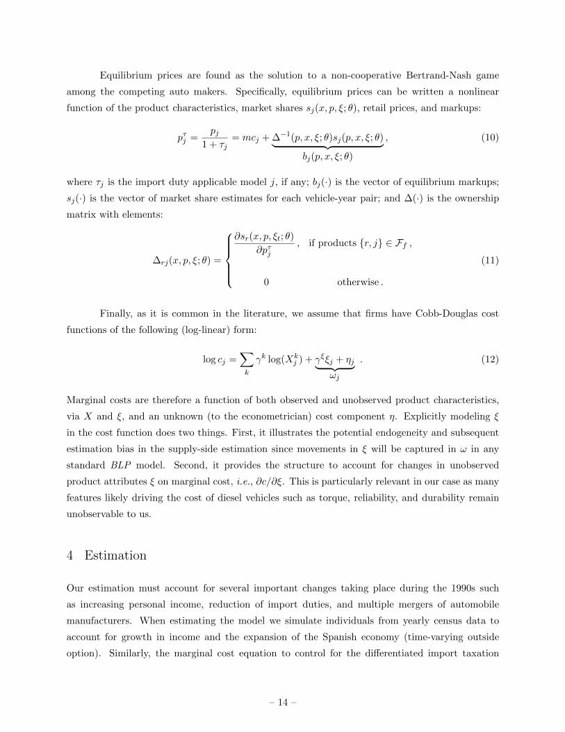
Equilibrium prices are found as the solution to a non-cooperative Bertrand-Nash game

among the competing auto makers. Specifically, equilibrium prices can be written a nonlinear

function of the product characteristics, market shares sj(x, p, ξ; θ), retail prices, and markups:

pτj =pj

1 + τj= mcj + ∆−1(p, x, ξ; θ)sj(p, x, ξ; θ)︸ ︷︷ ︸

bj(p, x, ξ; θ)

, (10)

where τj is the import duty applicable model j, if any; bj(·) is the vector of equilibrium markups;

sj(·) is the vector of market share estimates for each vehicle-year pair; and ∆(·) is the ownership

matrix with elements:

∆rj(x, p, ξ; θ) =

∂sr(x, p, ξt; θ)

∂pτj, if products r, j ∈ Ff ,

0 otherwise .

(11)

Finally, as it is common in the literature, we assume that firms have Cobb-Douglas cost

functions of the following (log-linear) form:

log cj =∑k

γk log(Xkj ) + γξξj + ηj︸ ︷︷ ︸

ωj

. (12)

Marginal costs are therefore a function of both observed and unobserved product characteristics,

via X and ξ, and an unknown (to the econometrician) cost component η. Explicitly modeling ξ

in the cost function does two things. First, it illustrates the potential endogeneity and subsequent

estimation bias in the supply-side estimation since movements in ξ will be captured in ω in any

standard BLP model. Second, it provides the structure to account for changes in unobserved

product attributes ξ on marginal cost, i.e., ∂c/∂ξ. This is particularly relevant in our case as many

features likely driving the cost of diesel vehicles such as torque, reliability, and durability remain

unobservable to us.

4 Estimation

Our estimation must account for several important changes taking place during the 1990s such

as increasing personal income, reduction of import duties, and multiple mergers of automobile

manufacturers. When estimating the model we simulate individuals from yearly census data to

account for growth in income and the expansion of the Spanish economy (time-varying outside

option). Similarly, the marginal cost equation to control for the differentiated import taxation

– 14 –

faced by manufacturers depending on their national origin. Finally, we update matrix ∆rj every

year to match the ever changing ownership structure of this industry during the 1990s and correctly

define the multi-product first-order profit maximization conditions of the equilibrium model to be

estimated.17

As we have argued, supply and demand of diesel vehicles is likely to be driven by prod-

uct characteristics such as torque ratio or reliability that might be observable to manufacturers,

learned by consumers, but remain unobserved for econometricians. The common practice in the

BLP literature is to assume that all product characteristics are exogenous while price is not and

then construct price instruments using functions of the product characteristics. However, these

unobservable product characteristics are likely correlated with other observable vehicle attributes.

This is true even in a static frameworks but in our case product characteristics change rapidly and

diesels are fast improving during the decade, which suggest that this correlation among attributes

will be even more likely to happen.

In our data, we observe that the product characteristics embodied in the car models offered

by firms do not appear to be random. Rather, we documented an increasing number of diesel

vehicles in the choice set, e.g., Figures 2 and 3, as well as cars becoming larger, heavier, and more

fuel efficient, etc during the 1990s, e.g., Figure 4. Consequently, assuming product characteristic

exogeneity is not appropriate in our context. Instead, we propose an alternative estimation strategy

which allows for endogenous product characteristics and uses the firms’ first-order conditions for

profit maximization to identify the structural demand and supply parameters. Specifically, we

consider the case where firms choose vehicle size, horsepower/weight ratio, and fuel efficiency as

well as the unobserved component, ξ. This allows us to account for changes in the demand valuation

and cost of diesel vehicles over time as captured via ξ.

4.1 The GMM Estimator

We estimate the structural parameters of the model by generalized method of moments (gmm) as

in Hansen (1982). Define the parameter vector Θ = [β,Σ,Π]. First, we solve for the mean utilities

δ(θ) using the standard contraction mapping outlined in Appendix I of BLP. Next we solve for

the implied markups bjt and use price data to construct marginal costs, assuming a pure strategy

Bertrand-Nash equilibrium. Next, we recover γ by regressing log marginal costs on the observable

(e.g., size) and unobservable (ξ) product characteristics as well as a set of controls such as fuel

type, a time trend, and brand (e.g., Audi) and segment (e.g., luxury) fixed effects. Our identifying

assumption is that the remaining error constitutes i.i.d. cost shocks which are uncorrelated with

17See Table A.1 in Appendix A for further details on import tariffs and mergers in the European automobile industryduring the 1990s.

– 15 –

the product characteristics and controls. This is a reasonable assumption since firms in the model

take the product set, including fuel type, as given.18 With the supply estimates at hand we then

construct the structural error εkj (Θ) defined by equations (8) as follows:

εkj (θ) = sj(θ)×∂[pτj − cj(θ)]

∂xkj+∑r∈Jf

[prτ − cr(θ)]×∂sr(θ)

∂xkj. (13)

The evaluation of the response of demand for all products of each firm to each change in product

characteristics makes this task particularly computationally-intensive as it requires solving repeat-

edly for the equilibrium price responses due to changes in product characteristics in addition to

evaluating numerically the multiple integrals of equation (9).

Profit-maximization requires that in each period t the expectation of the structural error ε

conditional on product characteristics equals zero for all products j ∈ Ff and characteristics k, i.e.,

E[εkj,t(θ)|X,W,ω] = 0). Since any function of the demand and supply characteristics X,W are valid

instruments, the set of potential instruments is large. Chamberlain (1987) shows the “optimal”

(i.e., most efficient) instruments are:

Hkj (θ) = E

[∂εkj (θ)

∂θ

∣∣∣X,W,ω] . (14)

The logic behind these instruments is straightforward: they place relatively more weight on obser-

vations that are responsive to changes in the estimates of θ. We solve for the value of the GMM

objective function conditional on θ by interacting the structural errors (13) with the identifying

moment conditions (14) as follows:

θ? = argminθ

G(θ)′A−1G(θ) , (15)

where G(θ) ≡ E[H(θ)⊗ ε] and A−1 is a positive-semidefinite weighting matrix that exists because

there are (K + 1) instruments for each element of θ. In constructing the weighting matrix, we

allow for the structural errors ε within a car model to be correlated across characteristics and

time. Consistent estimation of θ∗ requires updating both the instruments H and the weight matrix

A−1. To improve efficiency of the estimation we implement the iterative gmm estimator of Hansen,

Heaton and Yaron (1996). Thus, we obtained our parameter estimates by gmm where the estimator

exploits the fact that at the true value of parameters θ?, the instruments H are orthogonal to the

errors ε(θ?), e.g., E [H ⊗ ε(θ?)] = 0. We repeatedly update the weighting matrix A−1 until the

18Alternatively, we could have relaxed our OLS assumption and allowed for correlation between η and the productcharacteristics, including γ in θ and recovered these point estimates via gmm. Since it is difficult to identify areason for such a correlation once accounting for ξ, we chose our current approach which simplifies the estimationby decreasing the size of the parameter space. See Appendix B for details.

– 16 –

estimates of θ converge. To ensure the robustness of our results we employed a state-of-the-art

estimation algorithm (KNITRO) shown to be effective with this class of models; considered a large

variety of initial conditions; and used the strict inner-loop convergence criterion for calculating the

mean utility δ suggested by Dube, Fox and Su (2012).

This model represents a complex, nonlinear mapping from parameters to data. While

there is no clear one-to-one mapping between a parameter and a specific moment in the data, the

intuition into how data variation identifies different components of θ is as follows. Variation in

prices conditional on similar product characteristics identifies the product price elasticities while

cross-price elasticities are identified by differential changes in prices and quantities across products

with similar characteristics. Variation between product characteristics and sales pins down the mean

utility parameters (β) so diesel market share conditional on other product characteristics identifies

consumer preferences for diesel engines (βdiesel). The interaction between product characteristics

(e.g., price) and distribution of demographics identifies the interaction coefficient (Π). Variation

in the product set, product characteristics (e.g., size), prices, and quantities identifies the random

coefficients (σ). Lastly, the Bertrand-Nash equilibrium plus variation in price elasticities conditional

on product characteristics identifies marginal costs (γ).

4.2 Estimation Results

We estimate the model using the 1992-2000 sample period. Demand includes a measure of automo-

bile performance, horsepower divided by weight (hpw); exterior dimensions (size); and fuel cost of

driving, (kpe), with units defined in the caption to Table 1. All these variables includes a random

coefficient as well as diesel to generate substitution within the diesels and constant to capture

changes in substitution patterns due to the increasing product set.

On the supply side, the log of marginal cost of production is made a function of the type

of fuel, diesel; logs of product characteristics (hpw, weight, size, c90); a time trend aimed at

capturing potential efficiency gains, trend; and the unobservable attribute, ξ. In addition to the

reported estimates, the cost equation also included brand-specific and segment fixed effects. We

further allow for small differences between the demand and supply characteristics, including c90 in

the supply equation to account for the cost of improving a purely technical measure of fuel efficiency

while kpe, which includes the effect of fluctuations in the price of oil, independent of production

technology is included in the demand specification. Consequently, audi’s choice of fuel efficiency

for a gasoline A4 impacts its cost directly as measured by c90, but demand for A4’s will also be

influenced by changes in the price of gasoline due to economic factors outside of audi’s control.

Hence, we include kpe in the demand rather than in the supply equation. Similarly, changes in the

price of steel are allowed to impact hpw and size in supply but not demand.

– 17 –

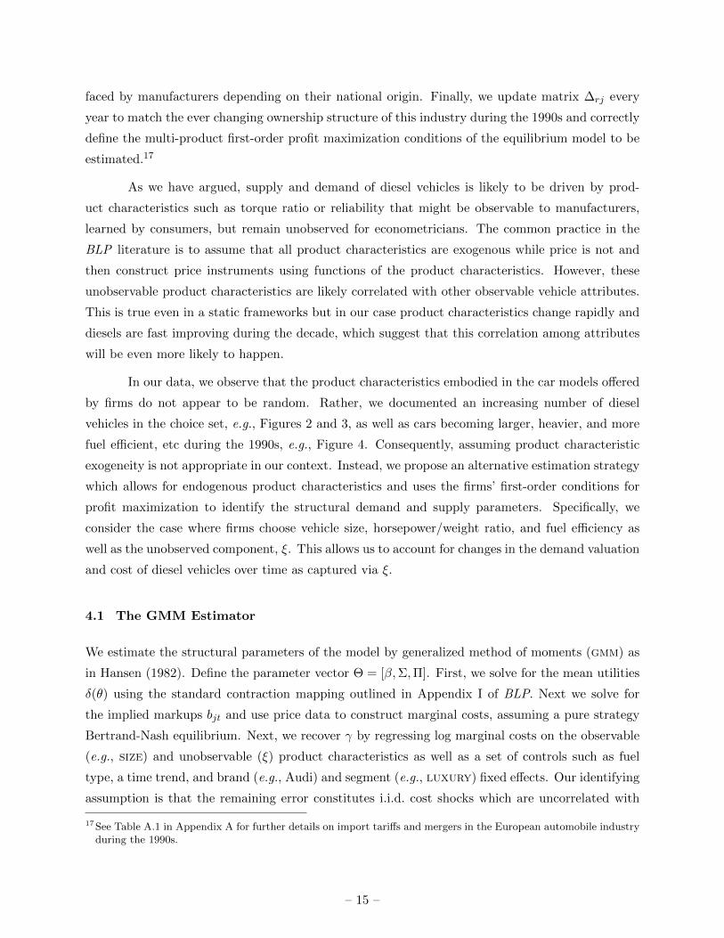
Table 2: Demand and Supply Estimates

Variable Coefficient Rob. SE Variable Coefficient Rob. SE

Mean Utility (β) Cost (γ)

kpe 0.2679 (0.3290) c90 0.1311 (0.0260)∗∗∗

size −13.2042 (0.6000)∗∗∗ size 0.8429 (0.0497)∗∗∗

hpw 1.5288 (0.4961)∗∗∗ hpw 0.3558 (0.0187)∗∗∗

constantb 5.7410 (0.2243)∗∗∗ constant 0.3964 (0.0761)∗∗∗

dieselb −2.3586 (0.5275)∗∗∗ diesel 0.1948 (0.0087)∗∗∗

dieselb93 0.7559 (0.6620) trend 0.0137 (0.0013)∗∗∗

dieselb94 2.2892 (0.6524)∗∗∗ ξ 0.0428 (0.0014)∗∗∗

dieselb95 2.0952 (0.6377)∗∗∗

dieselb96 3.0923 (0.6308)∗∗∗

dieselb97 3.7642 (0.6389)∗∗∗

dieselb98 2.3827 (0.6428)∗∗∗

dieselb99 3.5044 (0.6495)∗∗∗

dieselb00 2.2448 (0.6684)∗∗∗

non-eub −1.5035 (0.1882)∗∗∗

Standard Dev. (σ) Interactions (Π)

kpe 3.1142 (0.2649)∗∗∗ Price/Income −16.8963 (0.8800)∗∗∗

size 1.4304 (0.9971)

hpw 1.4671 (0.5383)∗∗∗

constant 2.8582 (0.0274)∗∗∗

diesel 2.1196 (0.0493)∗∗∗

Elasticity Statistics Margin Statistics (%)

- Average 8.7 - Average 12.9- Maximum 20.8 - Maximum 20.0- Minimum 5.4 - Minimum 6.3

Estimation Statistics

Number of observations 1,740Simulated agents per year 5,000J-statistic (df) 116.8 (27)

Robust standard errors in parentheses. Significant estimates with p-values less than 0.1, 0.05, and 0.01 areidentified with ∗, ∗∗, and ∗∗∗, respectively. Cost fixed effects for brand and segment not reported. b Estimatesbased on projecting the estimated values of the demand unobservable ξ on other demand characteristics,including segment fixed effects and a time trend. “Margin” defined as 100 × p−c

pwhere price excludes import

tariffs, if applicable. Equilibrium prices account for year-specific ownership structure as reported in Table A.1in Appendix 2.

The gmm estimation generates a 1, 740 × 1 vector of unobserved product characteristics.

We projected this vector onto a set of dummies to identify systemic patterns in demand. As this

time period covers the diffusion of diesel vehicles, we include a diesel dummy as well as a nonlinear

time interaction with diesel in order to capture the evolution of preferences in favor of the new

– 18 –

technology (in addition to non-reported segment fixed effects and a time trend). Finally, we added

the non-eu dummy to account for differences in valuation of the recently introduced Asian imports

in the European market.19

Table 2 reports the estimation results. Estimates are reasonable and congruent with the

descriptive evidence of the industry of Section 2. Starting with supply, diesels are more expensive

to manufacture than gasoline models. Marginal cost of production are also higher for fuel efficient

vehicles, larger, and more powerful cars. It appears that there are no important efficiency gains

occurring during the decade but rather a small long term increase in cost of production perhaps

driven by factors associated to the long term increase in sales of larger and more powerful vehicles

during the 1990s. Finally, observe that costs are also increasing in the unobserved quality attribute,

ξ. This may include better performance measured as reliability (or torque for diesel vehicles) as

well as cost associated to setting up dealership networks for Asian newcomers.

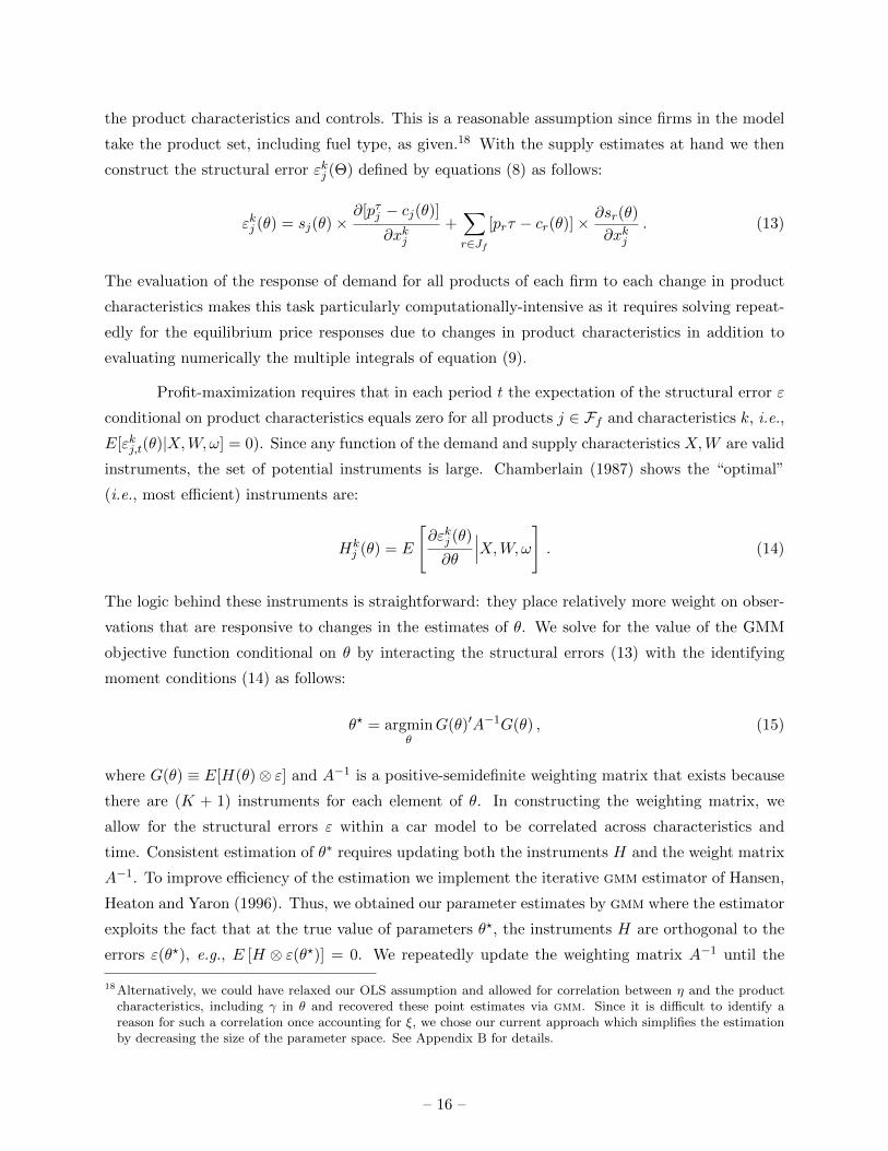
Figure 5: Production Costs Differences Across Brands(Reference: Renault)

-30%

-25%

-20%

-15%

-10%

-5%

0%

5%

10%

15%

20%

25%

30%

Alfa

Rom

eo

Aud

i

BM

W

Chr

ysle

r

Citr

oen

Dae

woo Fiat

Ford

Hon

da

Hyu

ndai

Kia

Lanc

ia

Maz

da

Mer

cede

s

Mits

ubis

hi

Nis

san

Ope

l

Peu

geut

Ren

ault

Rov

er

Saa

b

Sea

t

Sko

da

Suz

uki

Toyo

ta

Vol

ksw

agen

Vol

vo

Figure 5 depicts the non-reported, cost related, brand fixed effects relative to the Spanish

market leader, renault. Results are very reasonable, capturing the common perception of the

automobile market in Spain. German upscale brands audi, bmw, and mercedes, are among the

most expensive to produce. Chrysler (U.S. based) and Asian imports are quite competitive, with

Korean imports daewoo, hyundai, and kia, averaging a 25% relative cost advantage. European

19Not reported is a small, positive but insignificant seat indicator intended to capture any potential home biaseffect in Spanish drivers’ automobile purchasing decisions. In addition we also considered the aggregate output ofeach model in the European market aggregating sales by model (not distinguishing by fuel type) from Belgium,France, Germany, Italy and United Kingdom to Spanish sales using Frank Verboven’s data available at http:

//www.econ.kuleuven.be/public/ndbad83/frank/cars.htm. This measure of scale was never significant though,implying that automobile manufacturers enjoy Europe-wide constant returns to scale.

– 19 –

manufacturers with lower unit costs of production than renault, include the Czech brand skoda

and the old Spanish brand seat, both of them acquired by volkswagen to sell low quality versions

of their vehicles targeting lower income customers. Another interesting case of relatively low cost

of production is ford, which produces most of its smaller European models in a large plant located

in Spain. These results reassure us that our specification is reasonable and that our estimates will

be helpful in evaluating meaningful counterfactuals.

As for demand, Table 2 shows that it is downward slopping and always elastic, with

an average 8.7 price elasticity that in combination with the cost estimates leads to an average

13% margin for the Spanish automobile industry during the 1990s. There is however substantial

heterogeneity, with margins as low as 6% and as high as 20%. This wide range of margins are due to

heterogeneous valuation of cars’ characteristics at a moment in time, the evolution of preferences

over time, and the changing product offering over the decade.20 Figure 6 shows that average

margins, both of gasoline and diesel vehicles, remain quite stable, only decreasing very slightly

during the 1990s. In the case of diesel vehicles this margin reduction is more pronounced at the

beginning of the decade when the number of diesel models available increases significantly. For

both engine types, the dispersion of margins is substantially larger during the last three years of

the sample.

Figure 6: Evolution of Price-Cost Margins

0

5

10

15

20

25

Mar

gin

(PC

M)

1992 1993 1994 1995 1996 1997 1998 1999 2000excludes outside values

(a) Diesel Vehicles

0

5

10

15

20

25

Mar

gin

(PC

M)

1992 1993 1994 1995 1996 1997 1998 1999 2000excludes outside values

(b) Gasoline Vehicles

Estimates of Table 2 show that Spanish drivers mostly value smaller European cars deliv-

ering high performance (negative size, negative non-eu, and positive hpw). The negative sign of

non-eu is an empirical regularity in the international trade literature and is commonly referred to

as the “home bias” effect. Since our focus is on a specific industry rather than a set of bilateral

trade flows across many sectors, we can provide a more detailed interpretation. At this time,

Asian imports were first sold in the European market and were considered low quality, fuel efficient

20Although ignoring the distinction between diesel and gasoline models, Moral and Jaumandreu (2007) show thatdemand elasticities are smaller but also very heterogeneous across market segments and product life cycle.

– 20 –

alternatives to European vehicles but they lacked both brand recognition as well as a widespread

network of dealerships for maintenance. Thus, the negative sign of non-eu is not surprising.

On average, fuel cost does not rank high among Spanish drivers’ concerns (insignificant

kpe) as fuel prices remain quite stable until the end of the decade, precisely when jobs and personal

income is growing at record rates. Yet, there exists very significant heterogeneity of preferences

regarding fuel cost of driving (large positive σkpe). As for performance, tastes vary but the vast

majority of drivers favor high hp to weight ratios (significant but relatively small σsize). There

is however little heterogeneity regarding the preference for small vehicles (insignificant σsize).

Notice that diesel vehicles are not particularly valued at the beginning of the 1990s. How-

ever, during the economic growth phase of the second half of the decade, drivers clearly favored

them. The interaction of the nonlinear time trend and the diesel dummy captures this change

in preferences in favor of diesel vehicles. It is therefore likely that consumers become increasingly

aware of the features of diesel vehicles as they encounter them more frequently on the road.21

These results show that consumers’ perception of diesels evolves favorably over the decade as diesel

vehicles become more widespread.

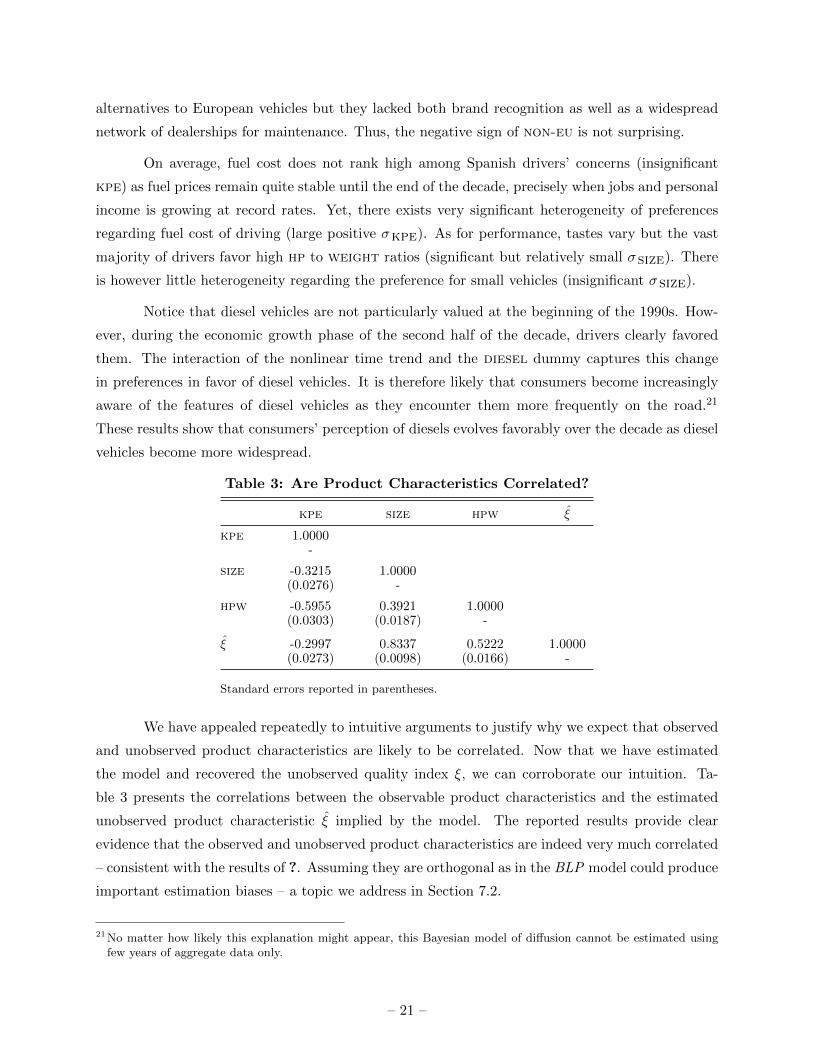
Table 3: Are Product Characteristics Correlated?

kpe size hpw ξ

kpe 1.0000-

size -0.3215 1.0000(0.0276) -

hpw -0.5955 0.3921 1.0000(0.0303) (0.0187) -

ξ -0.2997 0.8337 0.5222 1.0000(0.0273) (0.0098) (0.0166) -

Standard errors reported in parentheses.

We have appealed repeatedly to intuitive arguments to justify why we expect that observed

and unobserved product characteristics are likely to be correlated. Now that we have estimated

the model and recovered the unobserved quality index ξ, we can corroborate our intuition. Ta-

ble 3 presents the correlations between the observable product characteristics and the estimated

unobserved product characteristic ξ implied by the model. The reported results provide clear

evidence that the observed and unobserved product characteristics are indeed very much correlated

– consistent with the results of ?. Assuming they are orthogonal as in the BLP model could produce

important estimation biases – a topic we address in Section 7.2.

21No matter how likely this explanation might appear, this Bayesian model of diffusion cannot be estimated usingfew years of aggregate data only.

– 21 –

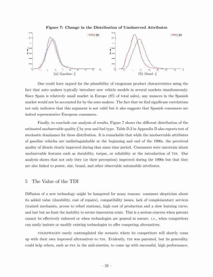
Figure 7: Change in the Distribution of Unobserved Attributes

(a) Gasoline: ξ (b) Diesel: ξ

One could have argued for the plausibility of exogenous product characteristics using the

fact that auto makers typically introduce new vehicle models in several markets simultaneously.

Since Spain is relatively small market in Europe (8% of total sales), any nuances in the Spanish

market would not be accounted for by the auto makers. The fact that we find significant correlations

not only indicates that this argument is not valid but it also suggests that Spanish consumers are

indeed representative European consumers.

Finally, to conclude our analysis of results, Figure 7 shows the different distribution of the

estimated unobservable quality ξ by year and fuel type. Table D.2 in Appendix D also reports test of

stochastic dominance for these distribution. It is remarkable that while the unobservable attributes

of gasoline vehicles are undistinguishable at the beginning and end of the 1990s, the perceived

quality of diesels clearly improved during that same time period. Consumers were uncertain about

unobservable features such as durability, torque, or reliability at the introduction of tdi. Our

analysis shows that not only they (or their perception) improved during the 1990s but that they

are also linked to power, size, brand, and other observable automobile attributes.

5 The Value of the TDI

Diffusion of a new technology might be hampered for many reasons: consumer skepticism about

its added value (durability, cost of repairs), compatibility issues, lack of complementary services

(trained mechanics, access to refuel stations), high cost of production and a slow learning curve,

and last but no least the inability to secure innovation rents. This is a serious concern when patents

cannot be effectively enforced or when technologies are general in nature, i.e., when competitors

can easily imitate or modify existing technologies to offer competing alternatives.

volkswagen surely contemplated the scenario where its competitors will shortly come

up with their own improved alternatives to tdi. Evidently, tdi was patented, but its generality,

could help others, such as psa in the mid-nineties, to come up with successful, high performance,

– 22 –

diesel-based, engine alternatives. A not so difficult process of reverse engineering might have allowed

competitors to limit volkswagen’s ability to appropriate the rents necessary to develop the tdi

engine, therefore questioning the wisdom of such innovation strategy in the first place.22

Figure 8: Importance of Diesels to Volkswagen Group’s Profits (Spain)

0

50

100

150

200

250

300

350

400

450

1992 1993 1994 1995 1996 1997 1998 1999 2000

(a) Profit (Millions)

0%

5%

10%

15%

20%

25%

30%

35%

40%

45%

50%

55%

60%

65%

1992 1993 1994 1995 1996 1997 1998 1999 2000

(b) Diesel Share of Profits

A revealed preference argument suffice to conclude that despite this imitation, tdi must

have been a very profitable initiative as it was still sold many years after its invention and others

entered this apparently very profitable segment. Figure 8(a) demonstrates that volkswagen was

indeed able to generate a lot of profit from the tdi and that tdi profits grew rapidly over the

decade, while Figure 8(b) indicates that sales of tdi became an increasingly important contributor

to the auto maker’s profits. These figures are obviously limited to Spain but they include sales

and profits for audi, seat, skoda, and volkswagen vehicles. Profits will be much larger when

considering the whole European market.

That said, imitation by European auto makers undoubtedly had an impact on the value

of the tdi to volkswagen. In Table 4 we use the estimates of the model to conduct a couple

of counterfactuals that help us assess the importance of potential innovation rents captured by

volkswagen – or equivalently estimate how much business were other European auto makers able

to steal by imitating this general technology.

To evaluate the profitability of tdi for volkswagen, we make use of two counterfactu-

als. The “Benchmark” column summarizes the sales-averaged price, market share, sales-averaged

margins and profits originating from the diesel and gasoline segments in year 2000. The “No tdi”

counterfactual of Table 4 considers the possibility that diesels are either not allowed by regulators,

or were simply never developed by any automobile manufacturer. This would characterize any

market other than the European automobile market as diesels failed to succeed anywhere else than

22 It is the generality of this technology what allows it to be imitated and reused easily by other manufacturers, a goodexample of limited appropriability of profits of innovations of general purpose technologies that can be recombinedand reused in other applications. See Bresnahan (2010).

– 23 –

Table 4: Value of TDI Technology to Volkswagen (2000)

No tdi Benchmark Monopoly

Price (eThousand) 15.84 16.14 17.42- Diesel - 16.72 18.42- Gas 15.84 15.24 15.66

Market Share (%) 20.30 23.43 37.00- Diesel - 26.53 100.00- Gas 20.30 19.84 17.60

Margin (%) 14.51 13.73 17.95- Diesel - 13.29 19.04- Gas 14.51 14.40 16.05

Profit (eMillion) 432.25 679.13 1,211.84- Diesel 0.00 418.36 863.54- Gas 432.25 260.78 348.29

All numbers refer to year 2000. “Price” is in thousands of 1994 Euros. ‘Market Share” is thepercent share of cars sold in the respective category. “Margin” is defined as

(p−cc

)where price

includes tariffs. “Profit” is measured in millions of 1994 Euros.

in Europe. Under this scenario volkswagen’s overall profits are me247 lower despite the fact

that profits from the gasoline division grow by me171. This latter effect is due to the fact that

we consider the number of gasoline model constant. Thus, removing the whole set of fuel efficient

diesel vehicles allows manufacturers of gasoline models, including volkswagen, to increase their

sales and profits.

In order to determine how much of the innovation rents volkswagen was able to secure,

we need to evaluate another counterfactual where the tdi technology is assumed to be exclusive for

volkswagen and where competitors cannot come up with close substitutes in the diesel segment.

In the “Monopoly” counterfactual, volkswagen (including its affiliate brands) is the sole seller of

diesel vehicles. We thus recompute the equilibrium by removing all 2000 diesel models other than

those produced by the volkswagen group, which now enjoys monopoly power over that market

segment. Profits then become substantially larger for volkswagen under such scenario, up to

bne1.2, or about me533 higher. Profits from the diesel segment alone more than doubled, from

me418 to me864. It would be wrong to conclude that volkswagen was able to secure almost half

of the rents of innovation because comparing these two number ignores the effect that not having

diesel models available at all, or only sold by volkswagen has on profits through increased sales of

efficient gasoline models. Since firms produce a variety of products, the maximum innovation rents

is not only determined by the possibility of selling diesel vehicles or not, but also by the indirect

effect that demand may have on substitute gasoline models.

Thus, the maximum value of the innovation rents amount to me780, the difference between

volkswagen’s total profits of being a diesel monopolist and the scenario when diesels do not exists.

Therefore, starting from the “No tdi” scenario, we can compare the maximum total incremental

– 24 –

profits of being a monopolist me1212 – me432 = me780, with the incremental profits of the

benchmark scenario me679 - me432 = me247, to conclude that volkswagen is able to keep

31.7% of the potential rents of the tdi innovation under a much more strict patent protection or

less easily reusable technology. Competition is thus responsible for the dissipation of two thirds of

the innovation rents, which will benefit consumers in the form of lower prices and more products

to choose from. Table 4 also show that relative to a scenario where volkswagen was the solely

producer of diesel vehicles, prices of volkswagen’s gasoline models were about 2.5% lower while

volkswagen’s diesel models were almost 10% less expensive.

Figure 9: Volkswagen’s Rent Capture Across the Decade

-10%

-5%

0%

5%

10%

15%

20%

25%

30%

35%

1992 1993 1994 1995 1996 1997 1998 1999 2000

At the beginning of the 1990s volkswagen was not the leader of the Spanish market in

neither gasoline or diesel. renault, ford, and gm (better known as opel in continental Europe)

led the gasoline segment and citroen, peugeot, and renault the diesel segment. The diffusion

of diesels during the decade shook these rankings with renault still leading the gasoline segment

(although with half the sales) and the psa group dominating the diesel segment, e.g., see Figure D.1

in Appendix D. volkswagen was a close second top diesel seller thanks to the early acquisition of

the local producer seat. Because of this, Figure 9 shows that the share of potential rents captured

by volkswagen kept growing, during the decade. Only at the very beginning, in 1992, it appears

that the introduction of the tdi cannibalized profits from the gasoline segment.

A clear conclusion from Figure 8 and Table 4 is that the tdi was a valuable innovation for

volkswagen. In Appendix D we repeat the analysis of Table 4 for years 1992 and 2000 and all

automobile groups. Table D.4 shows that in 2000, psa, the local leader in the diesel segment, benefit

the most from the widespread acceptance of diesels among drivers, followed by volkswagen,

renault, gm, and ford. Only mercedes and non-eu auto makers saw their profits reduced

– 25 –

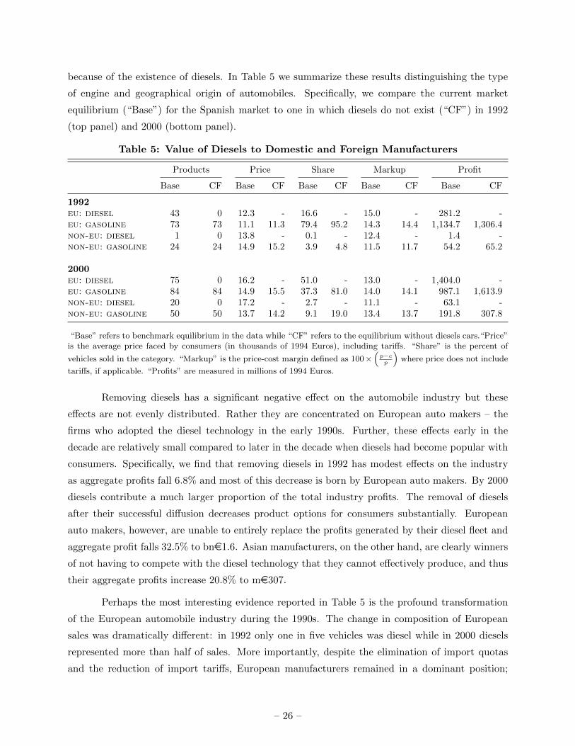
because of the existence of diesels. In Table 5 we summarize these results distinguishing the type

of engine and geographical origin of automobiles. Specifically, we compare the current market

equilibrium (“Base”) for the Spanish market to one in which diesels do not exist (“CF”) in 1992

(top panel) and 2000 (bottom panel).

Table 5: Value of Diesels to Domestic and Foreign Manufacturers

Products Price Share Markup Profit

Base CF Base CF Base CF Base CF Base CF

1992eu: diesel 43 0 12.3 - 16.6 - 15.0 - 281.2 -eu: gasoline 73 73 11.1 11.3 79.4 95.2 14.3 14.4 1,134.7 1,306.4non-eu: diesel 1 0 13.8 - 0.1 - 12.4 - 1.4 -non-eu: gasoline 24 24 14.9 15.2 3.9 4.8 11.5 11.7 54.2 65.2

2000eu: diesel 75 0 16.2 - 51.0 - 13.0 - 1,404.0 -eu: gasoline 84 84 14.9 15.5 37.3 81.0 14.0 14.1 987.1 1,613.9non-eu: diesel 20 0 17.2 - 2.7 - 11.1 - 63.1 -non-eu: gasoline 50 50 13.7 14.2 9.1 19.0 13.4 13.7 191.8 307.8

“Base” refers to benchmark equilibrium in the data while “CF” refers to the equilibrium without diesels cars.“Price”is the average price faced by consumers (in thousands of 1994 Euros), including tariffs. “Share” is the percent of

vehicles sold in the category. “Markup” is the price-cost margin defined as 100×(p−cp

)where price does not include

tariffs, if applicable. “Profits” are measured in millions of 1994 Euros.

Removing diesels has a significant negative effect on the automobile industry but these

effects are not evenly distributed. Rather they are concentrated on European auto makers – the

firms who adopted the diesel technology in the early 1990s. Further, these effects early in the

decade are relatively small compared to later in the decade when diesels had become popular with

consumers. Specifically, we find that removing diesels in 1992 has modest effects on the industry

as aggregate profits fall 6.8% and most of this decrease is born by European auto makers. By 2000

diesels contribute a much larger proportion of the total industry profits. The removal of diesels

after their successful diffusion decreases product options for consumers substantially. European

auto makers, however, are unable to entirely replace the profits generated by their diesel fleet and

aggregate profit falls 32.5% to bne1.6. Asian manufacturers, on the other hand, are clearly winners

of not having to compete with the diesel technology that they cannot effectively produce, and thus

their aggregate profits increase 20.8% to me307.

Perhaps the most interesting evidence reported in Table 5 is the profound transformation

of the European automobile industry during the 1990s. The change in composition of European

sales was dramatically different: in 1992 only one in five vehicles was diesel while in 2000 diesels

represented more than half of sales. More importantly, despite the elimination of import quotas

and the reduction of import tariffs, European manufacturers remained in a dominant position;

– 26 –

accounting for 96% of automobile sales in Spain in 1992 and only losing about 8% share to imports

by the end of the decade.23 But if diesels had not existed, for whatever the reason, Europeans

would have lost another 7% market share to imports. Thus, the existence and viability of the diesel

technology clearly benefited domestic European manufacturers.

So far we have shown that diesels were an incredibly profitable product for European auto

makers. A natural question then is why did foreign firms not offer diesels. The difference lies in

the fact that for European auto makers a significant portion of their profits came from European

consumers whereas Europe was a small market for foreign auto makers.24 This suggests that

the reason the tdi was invented and imitated by European firms is that diesel popularity was

fundamentally a European phenomenon so only firms which generated a significant percentage of

their profits from the European market were willing to spend the money to develop the technology.

Consequently, the competitive advantage offered by diesels resulted from the fact that European

firms were willing to spend the money to develop a product which catered to the idiosyncratic

tastes of European consumers.

6 Emissions Policies as Industry Protection

Using the model to measure the effects of removing all diesel vehicles from the European market

might, in most circumstances, be contemplated as a simple theoretical exercise. In this section

we present evidence that European regulatory policies on fuel and particularly emissions standards

could have realistically choked the diffusion of diesel vehicles in the early stages of its adoption. The

trade implication of such policies are significant – a near doubling of the share of imports from 11.8

to 19 percent. By not adopting such damaging policies, whether inadvertently or not, European

policymakers implicitly helped European manufacturers enhance their dominance in the domestic

market. To our knowledge this is the first time a structural equilibrium model of oligopoly industry

competition in differentiated products has been used to evaluate trade frictions, in particular the

trade protective impact of environmental regulation.

6.1 Vehicle Emissions Standards in the United States and Europe

We have thus far identified the generality of diesel technology as the main cause behind the success

of the diffusion of diesel vehicles in Europe in such a short period of time: the increased competition

23This compares to a 34% penetration of Asian in the United States in year 2000. See Automotive News MarketData Book (1980-2006).

24The percent of revenue from the European market for bmw, psa, renault, and volkswagen was 65%, 93%, 84%,and 74%, respectively, while for honda, mazda, and toyota the shares are substantially smaller – 11%, 10%, and8%, respectively (source: company 10-K SEC filings).

– 27 –

lowered the price of diesel vehicles, increased the supply of models for sale, and help dissipating

the innovation rents among economic agents. And yet, despite how easy imitation appears to be,

diesels almost disappeared in the U.S. during the same period of time. The common explanation

for the different evolution of these two large markets attributes the success of diesels in Europe to

the favorable tax treatment of the diesel fuels in Europe. In this section we put forward the novel

hypothesis that the different fate of diesels in Europe and the U.S. was instead due to the different

goals pursued by the environmental policies in the U.S. and in Europe. While Americans were

concerned mostly with reduction in emissions leading to acid rain, Europeans aimed at reducing

green house emissions.

Figure 10 illustrates the differences in emissions standards between the United States

and Europe in the year 2000.25 In the United States, the approval of the 1990 Clean Air Act

Amendments (CAAA) directed the U.S. Environmental Protection Agency (EPA) to, among many

other things, reduce acid rain produced by nitrogen oxide (NOx) and sulfur dioxide (SO2). The

EPA therefore chose a policy largely aimed at power generating plants which set emission reduction

goals (Title IV-A) and established a cap-and-trade system (Title V), but it also translated into an

ever more stringent NOx emission standards for light-duty vehicles (Title II-A).

Figure 10: Europe and U.S. Emissions Standards

0.07

0.4

0

0.1

0.2

0.3

0.4

0.5

0.6

0.7

0.8

0.9

1

US EU

NOx

0.01

0.04

0

0.02

0.04

0.06

0.08

0.1

0.12

0.14

0.16

0.18

0.2

US EU

PM

2.89

0.8

0

0.5

1

1.5

2

2.5

3

3.5

4

US EU

CO

330

224

0

50

100

150

200

250

300

350

400

US EU

CO2

Source: www.dieselforum.org. All statistics are for the year 2000 and are in grams per mile. “NOx” refers tonitrogen oxide limits; “PM” to particulate matter; “CO” carbon monoxide; and “CO2” carbon dioxide.

25European authorities set NOx and particulate matter (PM) standards for each vehicle while U.S. authorities seta fleet-wide limit. As for CO and CO2 emissions, these depend on fleet average fuel consumption standards andare reported in Figure 10 as realized fleet-wide levels. See Section IV of the 2001 report: “Demand for Diesels:The European Experience. Harnessing Diesel Innovation for Passenger Vehicle Fuel Efficiency and EmissionsObjectives” available at www.dieselforum.org.

– 28 –

European regulators took a different approach and chose a less stringent NOx emission

standard. While in 1994 U.S. Tier 1 standard allowed NOx emissions of 1 gram per mile (g/mi),

the Euro I standard was 1.55g/mi. By year 2000, the U.S. policy allowed only 0.07g/mi while the

Euro III standard set the NOx emission level at a far less demanding 0.4g/mi level.The fast diffusion

of diesel vehicles in the 1990s likely also enabled European authorities to choose more stringent

CO2 emission standards than the United States; the goals of local automobile manufacturers

and European environmental regulators were thus perfectly aligned. Were these differences in

environmental goals enough to explain the different evolution of diesels in the U.S. and Europe?

Absent any data on sales of automobiles by type of engine in the American market, we argue that

this is the case based on anecdotal evidence for the U.S. and counterfactual analysis for Europe.

The differences between the U.S. and European standards are significant for automobiles

since reducing NOx emissions is much harder for diesel engines as the three-way catalytic converters

used to reduce emissions in gasoline engines cannot cope with the high concentrations of NOx

generated by diesel engines (e.g., Canis 2012). Thus, rather than investing to redesign their diesel

engines to meet these stringent emission standards, volkswagen and mercedes chose to stop

selling their diesel models in the U.S. market in 1993 and 1994, respectively, precisely at the

time of the implementation of the U.S. emission standards mandated by the CAAA.26 Only in

2010 did the EPA finally address the issue of NOx emissions from diesel vehicles by requiring the

installation of an urea-based selective catalytic reduction that injects an aqueous solution into the

vehicles’ exhaust stream to “scrub” NOx emissions. Since then, auto makers have introduced more

diesel models into U.S. market, including those states that adhere to the even more demanding

California emission standards. All these circumstances suggest that the imposition of the these

emission standards amounted to a de facto ban of diesel vehicles in the U.S. market. Could then a

similar European emission policy have eliminated any chance of success for diesels in Europe?

6.2 Retrofitting Costs

We now focus on the likely cost of retrofitting diesel engines in order to make them comply with the

NOx emission standards set by the EPA. In so doing we test whether an alternative an emissions

policy like the one employed by the United States would have materially affected the European

industry. We show that meeting these regulatory standards is expensive and we can conclude that

such a shift in policy would have had effects commensurate with the results presented in Table 5.

26According to Stewart (2010), the NOx emissions level of the least polluting diesel model available in Canada,the volkswagen Jetta (known as Bora in Europe), was 0.915 and 0.927g/mi for the 1991 and 1997 year models,respectively. This indicates that the NOx emissions standards imposed by the EPA were indeed binding constraintsfor diesel vehicles since even the cleanest diesel models barely met the 1994 U.S. emission standards and wouldhave generated NOx emissions thirteen times greater than the 2000 limit.

– 29 –

For years, a technology to successfully capture NOx emissions at the tailpipe simply did

not exist. When it finally became available, in the late 2000s, it was still very expensive. By

the EPA’s own estimates in 2010, diesel engines could be retrofitted to comply with both EPA

and California NOx emission standards by means of a Lean NOx Catalyst at an estimated cost of

between $6,500 to $10,000 per vehicle. Lean NOx catalysts use diesel fuel injected into the exhaust

stream to create a catalytic reaction and reduce pollution. However, these catalysts still require

specific exhaust temperatures for appropriate NOx emission control performance, and on average

they reduce emissions up to a maximum of 40%. German manufacturers bmw and mercedes

were certified to be sold in all 50 states of the U.S. in 2009 only after equipping their new vehicles

with a Selective Catalytic Reduction System that injects a reductant (a urea-based solution) into

the exhaust stream where it reacts with a catalyst to convert NOx emissions to nitrogen gas and

oxygen. This system is more effective, reducing NOx emissions up to 75% but the EPA estimated

that its cost ranged between $10,000 and $20,000 per vehicle in 2010.27

Figure 11: Market Shares and Retrofitting Costs

EU: Gas

Non-EU: Gas

EU: Diesel

Non-EU: Diesel0

10

20

30

40

50

60

70

80

Mar

ket S

hare

(%

)

0 5 10 15 20 25

Retrofitting Expense (Thousands of Euro)(a) By Region, 1000e

Volkswagen

Non-EU

PSA

RenaultGMFord

FiatBMWMercedesRover0

5

10

15

20

25

Mar

ket S

hare

(%

)

0 5 10 15 20 25

Retrofitting Expense (Thousands of Euro)(b) By Firm, 1000e

Had this technology been available in the 1990s, retrofitting costs would have been even

higher. Figures 11(a) and 11(b) plots the results of using our estimates to recompute the market

equilibrium repeatedly after adding a wide range of retrofitting costs to the marginal cost of

production of diesels. The shaded area highlights the limits of the retrofitting cost region of the lean

and selective catalysts corrected for exchange rate and inflation. Figure 11(a) describes the effect

on market shares distinguishing by type of engine and geographical origin of manufacturers while

Figure 11(b) reports the combined market shares (gasoline & diesel) of each automobile group.

Figure 11(a) shows that a retrofitting cost of e3,300 for the lean catalyst in year 2000, the

NOx emission regulation has effectively reduced the diesel segment to a market niche comparable

to the diesel market penetration in Europe prior to the tdi innovation. The increase in production

27On retrofitting costs see Diesel Retrofit Devices. EPA’s National Clean Diesel Campaign, 2013. http://www.epa.

gov/cleandiesel/technologies/retrofits.htm

– 30 –

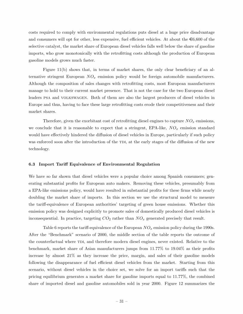
costs required to comply with environmental regulations puts diesel at a huge price disadvantage

and consumers will opt for other, less expensive, fuel efficient vehicles. At about the e6,600 of the

selective catalyst, the market share of European diesel vehicles falls well below the share of gasoline

imports, who grow monotonically with the retrofitting costs although the production of European

gasoline models grows much faster.

Figure 11(b) shows that, in terms of market shares, the only clear beneficiary of an al-

ternative stringent European NOx emission policy would be foreign automobile manufacturers.

Although the composition of sales changes with retrofitting costs, most European manufacturers

manage to hold to their current market presence. That is not the case for the two European diesel

leaders psa and volkswagen. Both of them are also the largest producers of diesel vehicles in

Europe and thus, having to face these large retrofitting costs erode their competitiveness and their

market shares.

Therefore, given the exorbitant cost of retrofitting diesel engines to capture NOx emissions,

we conclude that it is reasonable to expect that a stringent, EPA-like, NOx emission standard

would have effectively hindered the diffusion of diesel vehicles in Europe, particularly if such policy

was enforced soon after the introduction of the tdi, at the early stages of the diffusion of the new

technology.

6.3 Import Tariff Equivalence of Environmental Regulation

We have so far shown that diesel vehicles were a popular choice among Spanish consumers; gen-

erating substantial profits for European auto makers. Removing these vehicles, presumably from

a EPA-like emissions policy, would have resulted in substantial profits for these firms while nearly

doubling the market share of imports. In this section we use the structural model to measure

the tariff-equivalence of European authorities’ targeting of green house emissions. Whether this

emission policy was designed explicitly to promote sales of domestically produced diesel vehicles is

inconsequential. In practice, targeting CO2 rather than NOx generated precisely that result.

Table 6 reports the tariff-equivalence of the European NOx emission policy during the 1990s.

After the “Benchmark” scenario of 2000, the middle section of the table reports the outcome of

the counterfactual where tdi, and therefore modern diesel engines, never existed. Relative to the

benchmark, market share of Asian manufacturers jumps from 11.77% to 19.04% as their profits

increase by almost 21% as they increase the price, margin, and sales of their gasoline models

following the disappearance of fuel efficient diesel vehicles from the market. Starting from this

scenario, without diesel vehicles in the choice set, we solve for an import tariffs such that the

pricing equilibrium generates a market share for gasoline imports equal to 11.77%, the combined

share of imported diesel and gasoline automobiles sold in year 2000. Figure 12 summarizes the

– 31 –

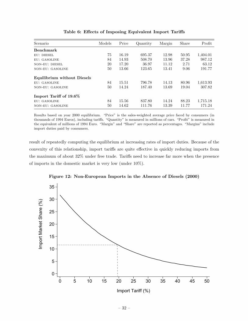
Table 6: Effects of Imposing Equivalent Import Tariffs

Scenario Models Price Quantity Margin Share Profit

Benchmarkeu: diesel 75 16.19 695.37 12.98 50.95 1,404.01eu: gasoline 84 14.93 508.70 13.96 37.28 987.12non-eu: diesel 20 17.20 36.97 11.12 2.71 63.12non-eu: gasoline 50 13.66 123.65 13.41 9.06 191.77

Equilibrium without Dieselseu: gasoline 84 15.51 796.78 14.13 80.96 1,613.93non-eu: gasoline 50 14.24 187.40 13.69 19.04 307.82

Import Tariff of 19.6%eu: gasoline 84 15.56 837.80 14.24 88.23 1,715.18non-eu: gasoline 50 14.62 111.76 13.39 11.77 171.24

Results based on year 2000 equilibrium. “Price” is the sales-weighted average price faced by consumers (inthousands of 1994 Euros), including tariffs. “Quantity” is measured in millions of cars. “Profit” is measured inthe equivalent of millions of 1994 Euro. “Margin” and “Share” are reported as percentages. “Margins” includeimport duties paid by consumers.

result of repeatedly computing the equilibrium at increasing rates of import duties. Because of the

convexity of this relationship, import tariffs are quite effective in quickly reducing imports from

the maximum of about 32% under free trade. Tariffs need to increase far more when the presence

of imports in the domestic market is very low (under 10%).

Figure 12: Non-European Imports in the Absence of Diesels (2000)

0

5

10

15

20

25

30

35

40

Impo

rt M

arke

t Sha

re (%

)

0 5 10 15 20 25 30 35 40 45 50

Import Tariff (%)

– 32 –

We thus find that, in a world without diesels, a 19.6% import tariff would limit Asian

imports and lead to a similar market outcome as the European green house emission policy that

implicity favored the development of diesel vehicles. While large in its own right, this implied

tariff is roughly double the nominal tariff (10.3%) which existed at the time. Moreover, the market

penetration of Asian imports in Spain is similar to that of Europe overall and thus our analysis

could be vied as representative of the average protective power of this environmental regulation

across Europe. France is the most important outlier among large European automobile markets,

with Asian imports barely exceeding 5% market share in year 2000. For the French case, the

tariff equivalence of the European environmental policy reaches 35.3%. In summary, the emissions

policy employed by European regulators seems to have favored domestic auto makers as a de facto

non-tariff trade policy and further fostered the adoption of diesel vehicles in Europe during the

1990s.

7 Robustness

In this section we evaluate the robustness of our results. First, we evaluate the extent to which

favorable tax treatment of diesel fuels in Europe can explain the massive adoption of diesel vehicles

in Europe. Second, we discuss the appropriateness of our model and estimation approach; assessing

the qualitative and quantitative implications of assuming exogeneity of product characteristics.

7.1 Fuel Taxes and Diffusion of Diesel Vehicles

Our novel argument is that targeting CO2 emissions (or not targeting NOx) had far reaching

consequences for the successful diffusion. But relative to what? Wasn’t the diffusion of diesels the

result of favorable diesel fuel taxation? In this section we evaluate this commonly-held hypothesis,

including the effects of the new European fuel taxation principles implemented in 2013. We show

that favorable fuel taxation had an almost negligible effect on the market penetration of diesel

vehicles despite the popular belief. The change in fuel taxation principles is also inconsequential.

By comparison, the implications of the emission policy are dramatically more important.

Following the European Fuel Taxation Directive of the 1970s, diesel fuel received a favorable

treatment that has convinced many to conclude that the success of diesel vehicles in Europe was

due primarily to this favorable treatment of diesel fuel taxation. We argued in Section 2.2 that

the reduced diesel fuel tax rate was instrumental for the development of a diesel market niche

that eased the adoption of tdi and other improved diesel vehicles in the 1990s, two decades after

the European Fuel Tax Directive was adopted. We dispute, however, that by itself, the favorable

taxation of diesel fuels could explain the widespread adoption of diesel vehicles in Europe. In order

– 33 –

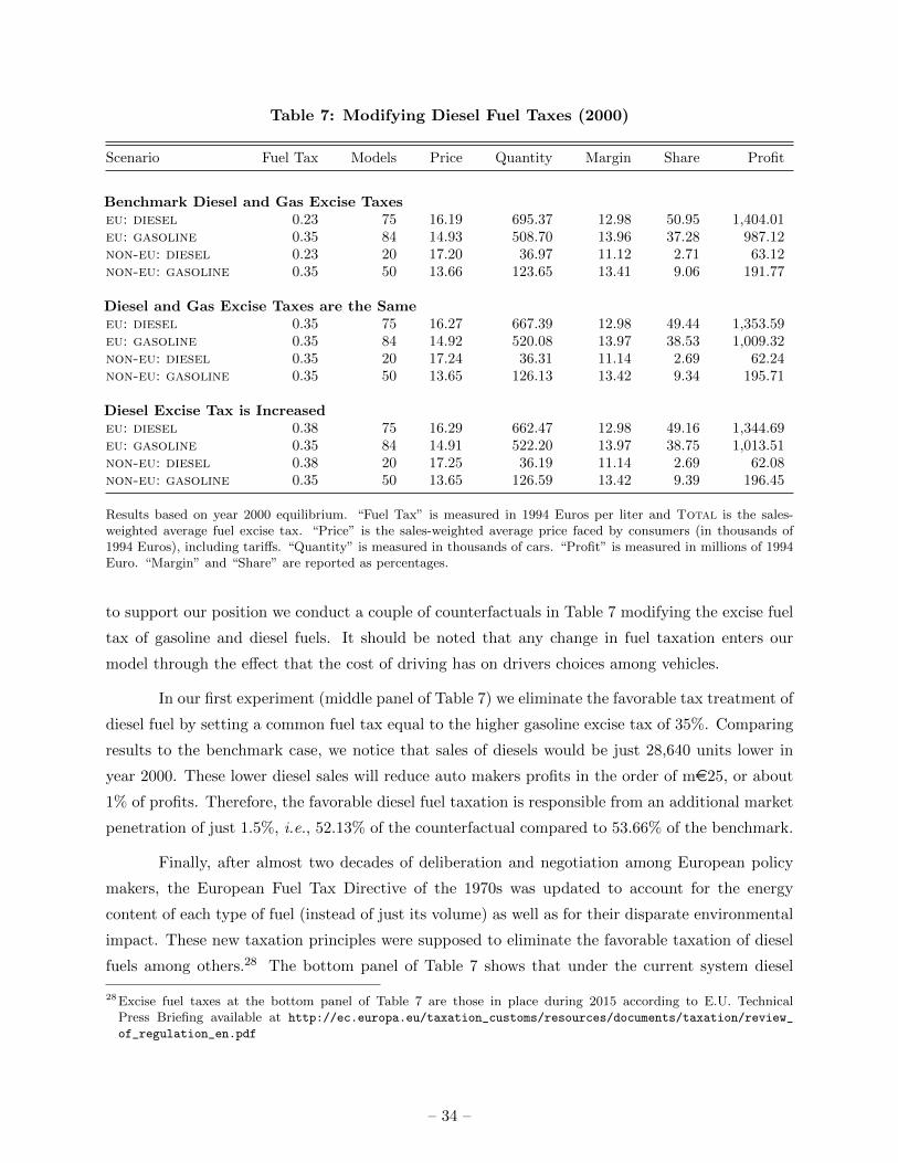
Table 7: Modifying Diesel Fuel Taxes (2000)

Scenario Fuel Tax Models Price Quantity Margin Share Profit

Benchmark Diesel and Gas Excise Taxeseu: diesel 0.23 75 16.19 695.37 12.98 50.95 1,404.01eu: gasoline 0.35 84 14.93 508.70 13.96 37.28 987.12non-eu: diesel 0.23 20 17.20 36.97 11.12 2.71 63.12non-eu: gasoline 0.35 50 13.66 123.65 13.41 9.06 191.77

Diesel and Gas Excise Taxes are the Sameeu: diesel 0.35 75 16.27 667.39 12.98 49.44 1,353.59eu: gasoline 0.35 84 14.92 520.08 13.97 38.53 1,009.32non-eu: diesel 0.35 20 17.24 36.31 11.14 2.69 62.24non-eu: gasoline 0.35 50 13.65 126.13 13.42 9.34 195.71

Diesel Excise Tax is Increasedeu: diesel 0.38 75 16.29 662.47 12.98 49.16 1,344.69eu: gasoline 0.35 84 14.91 522.20 13.97 38.75 1,013.51non-eu: diesel 0.38 20 17.25 36.19 11.14 2.69 62.08non-eu: gasoline 0.35 50 13.65 126.59 13.42 9.39 196.45

Results based on year 2000 equilibrium. “Fuel Tax” is measured in 1994 Euros per liter and Total is the sales-weighted average fuel excise tax. “Price” is the sales-weighted average price faced by consumers (in thousands of1994 Euros), including tariffs. “Quantity” is measured in thousands of cars. “Profit” is measured in millions of 1994Euro. “Margin” and “Share” are reported as percentages.

to support our position we conduct a couple of counterfactuals in Table 7 modifying the excise fuel

tax of gasoline and diesel fuels. It should be noted that any change in fuel taxation enters our

model through the effect that the cost of driving has on drivers choices among vehicles.

In our first experiment (middle panel of Table 7) we eliminate the favorable tax treatment of

diesel fuel by setting a common fuel tax equal to the higher gasoline excise tax of 35%. Comparing

results to the benchmark case, we notice that sales of diesels would be just 28,640 units lower in

year 2000. These lower diesel sales will reduce auto makers profits in the order of me25, or about

1% of profits. Therefore, the favorable diesel fuel taxation is responsible from an additional market

penetration of just 1.5%, i.e., 52.13% of the counterfactual compared to 53.66% of the benchmark.

Finally, after almost two decades of deliberation and negotiation among European policy

makers, the European Fuel Tax Directive of the 1970s was updated to account for the energy

content of each type of fuel (instead of just its volume) as well as for their disparate environmental

impact. These new taxation principles were supposed to eliminate the favorable taxation of diesel

fuels among others.28 The bottom panel of Table 7 shows that under the current system diesel

28Excise fuel taxes at the bottom panel of Table 7 are those in place during 2015 according to E.U. TechnicalPress Briefing available at http://ec.europa.eu/taxation_customs/resources/documents/taxation/review_

of_regulation_en.pdf

– 34 –

fuels are more heavily taxed than gasoline. Notice however that the much debated fuel taxation

reform has negligible effects when compared with the outcome of equal taxation of fuels by volume.

Relative to the benchmark case of 2000, the market penetration of diesels would be just 1.81%

lower. Relative to the scenario of equal excise taxation across fuels based on volume, the difference

is an almost nil 0.28% lower market share penetration of diesels.

7.2 Alternative Modeling Choices

In this section we address the implications and limitations of our modelling and estimation ap-

proach. Broadly, we view our paper as a step towards developing a more realistic model of the

automobile industry by providing useful insights into the quantitative price and profit implications

of attribute choices made by firms.29 Further, we believe our modeling choices are sufficient to

address the objectives in this paper, balancing a feasible extension of the BLP framework while

meeting the institutional limitations of our application.

First, an important attribute of the estimation approach is that we allow for but do not

impose correlation between observed and unobserved product characteristics – and we find that,

indeed, the estimated model does generate significant correlations among product characteristics.

Whether imposing zero correlation has significant qualitative and/ or qualitative implications to our

analysis is unclear ex ante. Table D.3 in Appendix D compares the estimation and counterfactual

results under both our current model (“MMT”) and a comparable, standard BLP estimation.

The results indicate that imposing product exogeneity leads to less precise estimates, particularly

for the random coefficients, and exaggerates the market power of automobile firms by triplicating

the estimated average price-cost margin of the industry. While using the standard BLP estima-

tion approach has little qualitative implications regarding our results (e.g., value of the tdi to

volkswagen, emissions policy as a non-tariff policy, et cetera), the quantitative implications are

significant.

Second, in the model, based on Petrin and Seo (2015), we assume that automobile man-

ufacturers first choose product characteristics based on their induced profits via future prices,

which happen to be determined non-cooperatively depending on the product positioning of all

automobile sold. An alternative would be to allow auto makers to choose prices and product

attributes simultaneously as prices might affect product design. Estimating such a model would be

difficult in our context as major releases of new model versions occur infrequently. Thus, we do not

consider the direct effect of product attributes on profits as in Fan (2013). Further, the data does

not contain “one clear event” leading to a total reorganization of the industry, including prices and

29Crawford (2012) presents a recent overview of the challenges of fully addressing the endogeneity of product attributesin discrete choice models of demand.

– 35 –

product attributes. In our case we observe multiple introduction of new products with changing

attributes over time. Thus, while this alternative approach would be interesting in many contexts,

it may not be appropriate for the automobile industry as auto makers design new vehicles several

years ahead of selling them. When choosing automobile attributes, observable or otherwise, they

account for the expected profits that those attribute choices may generate through future increased

markups. When cars are sold though, the primary strategic variable is price rather than product

attributes.

Lastly, it is worthwhile to discuss the rationale and potential implications of holding the

product set, including engine type, fixed in the model and estimation. It is perhaps more appro-

priate to think of the automobile industry as dynamic where manufacturers decide the timing of

introduction of new products and attributes, particularly diesel engines. Ignoring this relationship

has the potential to introduce bias into the estimates, though it is unclear what the size and

direction of those biases and the implications on our overall results would be.

Estimating such a dynamic model of product entry in the automobile industry would in-

crease the model’s complexity substantially and introduce new sources of uncertainty of which there

are no clear answers in the literature (e.g., modelling firm beliefs, multiple equilibria, et cetera).30

And unlike Sweeting (2013), our data covers one geographical market with limited demographic

variability and automobile attributes are not limited to few standardized categories but are mostly

continuous. Consequently, we have opted for a simpler model but one which is sufficiently flexible

to address the research goals of this paper. Further, the fact that diesel adoption in Spain occurred

earlier, though at a similar rate, than most European countries likely mitigates estimation bias

since it is unlikely that auto makers would have responded to increased Spanish demand for diesels.

8 Concluding Remarks

The goal in this paper was to measure the impact of a new diesel technology on the European

auto industry. To do so we estimated a structural oligopoly model of differentiated products where

we allowed for correlation between observed and unobserved product characteristics, finding that

the two sets of characteristics are indeed correlated. We also documented not only that there

is significant heterogeneity of preferences but that on average Spanish drivers do not only favor

smaller and high performance cars but also that their perception of diesel improved substantially

30The overwhelming majority of diesel vehicles are also offered as a gasoline version and the only difference betweenthe two versions is the engine type and all the characteristics associated with the engine. For example, a 1998audi A4 tdi is quicker (i.e., more torque), heavier, and more fuel efficient than a gasoline-powered A4 but itdoes not differ in size, interior space, creature comforts, et cetera. Consequently, a model with endogenous enginechoice would be similar to a dynamic model of product entry requiring firm beliefs about future profitability andinformation to identify the fixed costs of establishing the product.

– 36 –

during the 1990s. Widespread imitation of the tdi by European auto makers due to the generality

of the technology, enabled domestic firms to generate substantial profits from the technology

while limiting prices via increased competition, again favoring the adoption of diesel vehicles.

Despite the increased competition in the diesel segment, the tdi technology remained profitable for

volkswagen as the firm overcame the business stealing of it rivals to generate significant profits

from the technology and captured 32% of the potential innovation rents. We also find that, contrary

to popular belief, reduced fuel taxation was only responsible for just 1.5% fraction of diesel sales.

Instead, the greenhouse oriented emissions policy employed by European regulators had a much

more significant effect on the diesel technology’s widespread success.

Perhaps the most novel result of our paper is to show that seemingly non-trade policies

such as environmental standards can have important and quantitatively significant trade effects.

Regardless of whether the European pro-greenhouse emission policy was intended to favor the sales

of domestically produced diesel vehicles or not, we show that alternative NOx reduction policies

would have effectively halted the commercial success of diesel vehicles in the early 1990s, and,

given the large market share of diesels by year 2000, this policy amounted to an import tariff of

19.6% or approximately double the tariff employed by the European Union at the time. This is, to

the best of our knowledge, the first use of a structural equilibrium model of demand and industry

oligopoly competition to evaluate the trade effects of a non-tariff policy. Moreover, our results

illustrate that in an increasingly global economy, governments can effectively construct non-trade

oriented national policies, including environmental regulations, to protect domestic industries when

traditional trade policies are no longer available.

References

Bagwell, K. and R. W. Staiger (2001) “Domestic Policies, National Sovereignty and InternationalEconomics Institutions,” Quarterly Journal of Economics, Vol. 116, pp. 519–562.

Balcer, Y. and S. A. Lippman (1984) “Technological Expectations and Adoption of ImprovedTechnology,” Journal of Economic Theory, Vol. 34, pp. 292–318.

Barrett, G. F. and S. G. Donald (2003) “Consistent Test for Stochastic Dominance,” Econometrica,Vol. 71, pp. 71–104.

Berry, S., J. Levinsohn, and A. Pakes (1995) “Automobile Prices in Market Equilibrium,” Econo-metrica, Vol. 63, pp. 841–890.

(1999) “Voluntary Export Restraints on Automobiles: Evaluating Strategic Trade Policy,”American Economic Review, Vol. 89, pp. 400–430.

– 37 –

Bhagwati, J. and V. K. Ramaswami (1963) “Domestic Distortions, Tariffs, and the Theory ofOptimum Subsidy,” Journal of Political Economy, Vol. 71, pp. 44–50.

Bresnahan, T. F. (2010) “General Purpose Technology,” in B. H. Hall and N. Rosemberg eds.Handbook of the Economics of Innovation, Vol. II, New York, NY: North-Holland.

Busser, R. and Y. Sadoi (2004) “Japanese Automobile Makers in Europe and the Organizationof the Supply System,” in R. Busser and Y. Sadoi eds. Production Networks in Asia andEurope. Skill Formation and Technology Transfer in the Automobile Industry, New York,NY: Taylor & Francis.

Canis, B. (2012) “Why Some Fuel-Efficient Vehicles Are Not Sold Domestically,” report to congress,Congressional Research Service.

Chamberlain, G. (1987) “Asymptotic Efficiency in Estimation with Conditional Moment Restric-tions,” Journal of Econometrics, Vol. 34, pp. 305–334.

Chug, R., M. L. Cropper, and U. Narain (2011) “The Cost of Fuel Economy in the Indian PassengerVehicle Market,” Energy Policy, Vol. 39, pp. 7174–7183.

Crawford, G. S. (2012) “Endogenous Product Choice: A Progress Report,” International Journalof Industrial Organization, Vol. 30, pp. 315–320.

Deardorff, A. V. (1996) “An Economist’s Overview of the World Trade Organization,” WorkingPaper 388, Research Seminar in International Economics, University of Michigan.

Dube, J.-P., J. T. Fox, and C.-L. Su (2012) “Improving the Numerical Performance of Static andDynamic Aggregate Discrete Choice Random Coefficients Demand Estimation,” Economet-rica, Vol. 80, pp. 2231–2267.

Ederington, J. and J. Minier (2003) “Is Environmental Policy a Secondary Trade Barrier? AnEmpirical Analysis,” Canadian Journal of Economics, Vol. 36, pp. 1371–154.

Fan, Y. (2013) “Ownership Consolidation and Product Characteristics: A Study of the US DailyNewspaper Market,” American Economic Review, Vol. 103, pp. 1598–1628.

Greenwood, J. (1997) The Third Industrial Revolution: Technology, Productivity, and IncomeInequality, Washtington, DC: AEI Press.

Grigolon, L., M. Reynaert, and F. Verboven (2014) “Consumer Valuation of Fuel Costs and theEffectiveness of Tax Policy: Evidence from the European Car Market,” Discussion Paper10301, CEPR.

Hansen, L. P. (1982) “Large Sample Properties of Generalized Method of Moments Estimators,”Econometrica, Vol. 50, pp. 1029–1054.

Hansen, L. P., J. Heaton, and A. Yaron (1996) “Finite-Sample Properties of Some AlternativeGMM Estimators,” Journal of Business & Economic Statistics, Vol. 14, pp. 262–280.

Linn, J. (2014) “Explaining the Adoption of Diesel Fuel Passenger Cars in Europe,” Mimeo,Resources for the Future.

Manuelli, R. and A. Seshadri (2014) “Frictionless Technology Diffusion: The Case of Tractors,”American Economic Review, Vol. 104, No. 4, pp. 1368–1391.

– 38 –

Moral, M. J. and J. Jaumandreu (2007) “Automobile Demand, Model Cycle and Age Effects,”Spanish Economic Review, Vol. 9, pp. 193–218.

Nevo, A. (2000) “Mergers with differentiated Products: The Case of the Ready-to-Eat CerealIndustry,” RAND Journal of Economics, Vol. 31, pp. 395–421.

Oster, S. (1982) “The Diffusion of Innovation among Steel Firms: The Basic Oxygen Furnace,”Bell Journal of Economics, Vol. 13, pp. 45–56.

Petrin, A. (2002) “Quantifying the Benefits of New Products: The Case of the Minivan,” Journalof Political Economy, Vol. 110, pp. 705–729.

Petrin, A. and B. Seo (2015) “Identification and Estimation of Discrete Choice Models whenObserved and Unobserved Product Characteristics are Correlated,” Mimeo, University ofMinnesota.

Rose, N. L. and P. L. Joskow (1990) “The Diffusion of New Technologies: Evidence from theElectric Utility Industry,” RAND Journal of Economics, Vol. 21, pp. 354–373.

Schumpeter, J. A. (1950) Capitalism, Socialism, and Democracy, New York, NY: Harper & Row,3rd edition.

Staiger, R. W. (1995) “A Theory of Gradual Trade Liberalization,” in A. V. Deardorff, J. A.Levinsohn, and R. M. Stern eds. New Directions in Trade Theory, Ann Arbor, MI: TheUniversity of Michigan Press.

Stewart, S. J. (2010) “Collection of PM Emission Data from In-Use Light-Duty Diesel and GasolineVehicles,”Technical report, British Columbia Clean Air Research Fund Final Report, PacificVehicle Testing Technology, Ltd.

Sweeting, A. (2013) “Dynamic Product Positioning in Differentiated Product Markets: The Effectof Fees for Musical Performance Rights on the Commercial Radio Industry,” Econometrica,Vol. 81, pp. 1763–1803.

Thurk, J. (2014) “The Effects of Coordinating National Patent Policies,” Mimeo, University ofNotre Dame.

Verboven, F. (2002) “Quality-Based Price Discrimination and Tax Incidence: Evidence from Gaso-line and Diesel Cars,” RAND Journal of Economics, Vol. 33, pp. 275–297.

– 39 –

Appendix

A Spanish Data Sources

To control for household income distribution a thousand individuals are sampled each year from

the Encuesta Continua de Presupuestos Familiares (Base 1987 for years 1992-1997 and Base 1997

for years 1998-2000) conducted by INE, the Spanish Statistical Agency.31 The outside option varies

significantly during the 1990s due to the important recession between 1992 and 1994 and the very

fast growth of the economy and population (immigration) in the second half of the decade. We

also use these consumer surveys to set the size of the outside option for each year in our sample.

Starting with 1992, they are: 0.92, 0.94, 0.93, 0.93, 0.93, 0.92, 0.91, 0.89, and 0.89, respectively.

Fuel prices were also obtained from INE. In real 1994 euro-equivalent denominations per

liter, these are 0.445, 0.488, 0.490, 0.493, 0.543, 0.560. 0.530, 0.565, and 0.695 for diesel and

0.580, 0.628, 0.655, 0.678, 0.706, 0.724, 0.702, 0.737, and 0.875 for gasoline, for years 1992 to 2000,

respectively. As for the Spanish steel prices used as instruments for the cost equations, they are

obtained from the 2001 edition of Iron and Steel Statistics – Data 1991-2000 published by the

European Commission (Table 8.1).

For the analysis of demand we build a data set using prices and vehicle characteristics

as reported by La guıa del comprador de coches, ed. Moredi, Madrid. We select the price and

characteristics of the mid-range version of each model, i.e., the most popular and commonly sold.

Demand estimation also makes use of segment dummies. Other than the luxury segment, which

also includes sporty cars, our car segments follow the “Euro Car Segment” definition described

in Section IV of “Case No. COMP/M.1406 - Hyundai/Kia.” Regulation (EEC) No. 4064/89:

Merger Procedure Article 6(1)(b) Decision. Brussels, 17 March 1999. CELEX Database Document

No. 399M1406.

Until Spain ended its accession to the European Union transition period in 1992, it was

allowed to charge import duties on European products. Similarly, import duties for non-European

products converged to European levels. European imports paid tax duty of 4.4% in 1992, and

nothing thereafter. Non-European manufacturers had to pay 14.4% and 10.3%, respectively.

Thus, for the estimation of the equilibrium random coefficient discrete choice model of Table 2

we distinguish between prices paid by consumers and those perceived by manufacturers.

The other relevant factor that changes during the 1990s is the ownership structure of

automobile firms. During this decade fiat acquired alfa romeo and lancia; ford acquired

volvo; and gm acquired saab. bmw acquired rover in 1994 but sold it in May 2000 (with the

exception of the “Mini” brand) so these are treated as separate firms. Table A.1 describes the

ownership structure at the beginning and end of the decade.

31See http://www.ine.es/jaxi/menu.do?L=1&type=pcaxis&path=/t25/p458&file=inebase for a description ofthese databases in English.

– i –

Table A.1: Automobile Groups: 1992 vs. 2000

Year 1992 Year 2000

Firm Gasoline Diesel Owner Gasoline Diesel Owner

alfa romeo 5,038 64 alfa romeo 2,941 3,983 fiataudi 16,689 1,982 volkswagen 15,273 24,184 volkswagenbmw 17,855 1,906 bmw 13,683 15,838 bmwchrysler 1,243 – 5,941 2,389citroen 68,890 36,851 psa 46,420 111,694 psadaewoo – – 25,201 –fiat 35,677 5,733 fiat 30,557 17,967 fiatford 121,140 17,468 ford 55,268 57,013 fordhonda 4,805 – 8,782 1,072hyundai 2,704 – 30,150 3,590kia – – 9,778 1,387lancia 11,117 905 lancia 2,206 2,126 fiatmazda 3,064 – 2,205 1,480mercedes 9,352 4,129 mercedes 13,953 10,684 mercedesmitsubishi 3,041 – 3,660 1,013nissan 16,010 905 17,855 21,971opel 110,286 11,099 gm 66,488 75,418 gmpeugeot 61,323 35,494 psa 55,371 92,496 psarenault 147,907 27,448 renault 76,925 99,360 renaultrover 15,255 425 rover 10,173 8,491 roversaab 1,551 – saab 1,867 2,424 gmseat 85,773 11,787 volkswagen 58,072 109,447 volkswagenskoda 724 – skoda 5,003 10,385 volkswagensuzuki 2,058 – 3,250 486toyota 4,425 – 16,827 3,584volkswagen 50,561 5,471 volkswagen 47,125 50,296 volkswagenvolvo 10,179 – volvo 7,379 3,566 ford

Sales of vehicle by manufacturer and fuel type. “Owner” indicates the name of the automobilegroup with direct control on production and pricing. Those without a group are all non-European manufacturers and given their smaller size will be grouped under the non-eu labellater in the analysis.

B Estimation: Solving the Model

In this section we describe our algorithm to solve the model conditional on parameter guess θ =

[β,Σ,Π]. Since solving the model is independent across years, we drop the t subscripts for brevity.

The algorithm is as follows:

1. Compute δj using the contraction mapping described in (Berry et al., 1995, Appendix I).

2. Use µ(Σ,Π) and sijt(θ) to solve for the implied markups bj and use price data to construct

marginal costs.

3. Estimate γ by projecting ln(cj) onto the vector of cost shifters Z using ols. Since cost likely

varies by car segment (e.g., sedan) and brand (e.g., audi vs renault) we include segment

and brand fixed effects.

– ii –

4. Construct the structural error εkj defined as:

εkj (θ) = sj(θ)×∂(pτj − cj)

∂xkj+∑r∈Ff

(pτr − cr)×∂sr

∂xkj. (B.1)

(a) Use γ and the Cobb-Douglas specification of the marginal cost equation to generate∂cj∂Xk

j

.

(b) Evaluate the indirect (price-induced) market share response to attributes from:

∂sr

∂xkj=

∫νk

∫D

(βk + σkνk + πkD)× sij(1− sir)dPD(D)dPν(ν) +∑m∈Ff

∂sr∂pm

∂pm

∂xkj, r = j,

−∫νk

∫D

(βk + σkνk + πkD)× sijsirdPD(D)dPν(ν) +∑m∈Ff

∂sr∂pm

∂pm

∂xkj, otherwise .

(B.2)

(c) Solve for pτm∂xkj

. Recall the first-order condition for the price of product j is:

sj +∑r∈Fj

(pτr − cr)×∂sr∂pτj

= 0 . (B.3)

Total differentiation of (B.3) with respect to the vector of prices (dpτ ) and characteristic

k of product n (dxkn) yields:

J∑m=1

[∂sj∂pτm

+J∑r=1

T (r, j)∂2sr

∂pτj ∂pτm

× (pτr − cr) + T (m, j)∂sm∂pτj

]︸ ︷︷ ︸

g(j,m)

dpτm +

[∂sj∂xkn

+ 1If = j ∂cj∂xkn

]︸ ︷︷ ︸

h(j,n)

dxkn = 0 , (B.4)

where T (r, j) is equal to one when products r and j are produced by the same firm and

zero otherwise. Stack j conditions and define the matrix G with element g(j,m) and the

matrix H with element h(j, n). This implies that Gdpτ − Hfdxkn = 0 where Hn is the

nth column of H. Finally, we have dpτ

dxkn= G−1Hn, or more generally in matrix notation:

∆p = G−1H where ∆p(i, j) =∂pτi∂xkj

. In practice, we found that the ∂2sr∂pτj ∂p

τm

terms played

an insignificant role in constructing ∆p and that one could decrease computing time

significantly by setting these terms to zero.

(d) Define ∆s as the matrix of partial derivatives with element (i, j) = ∂si∂xkj

. The matrix ∆s

is an equilibrium object which is a function of ∆p which is, in turn, a function of ∆s.

Consequently, solving (B.4) requires solving for a fixed point. While we have no proof

that our operator is a contraction or that it results in a unique solution, we found that

– iii –

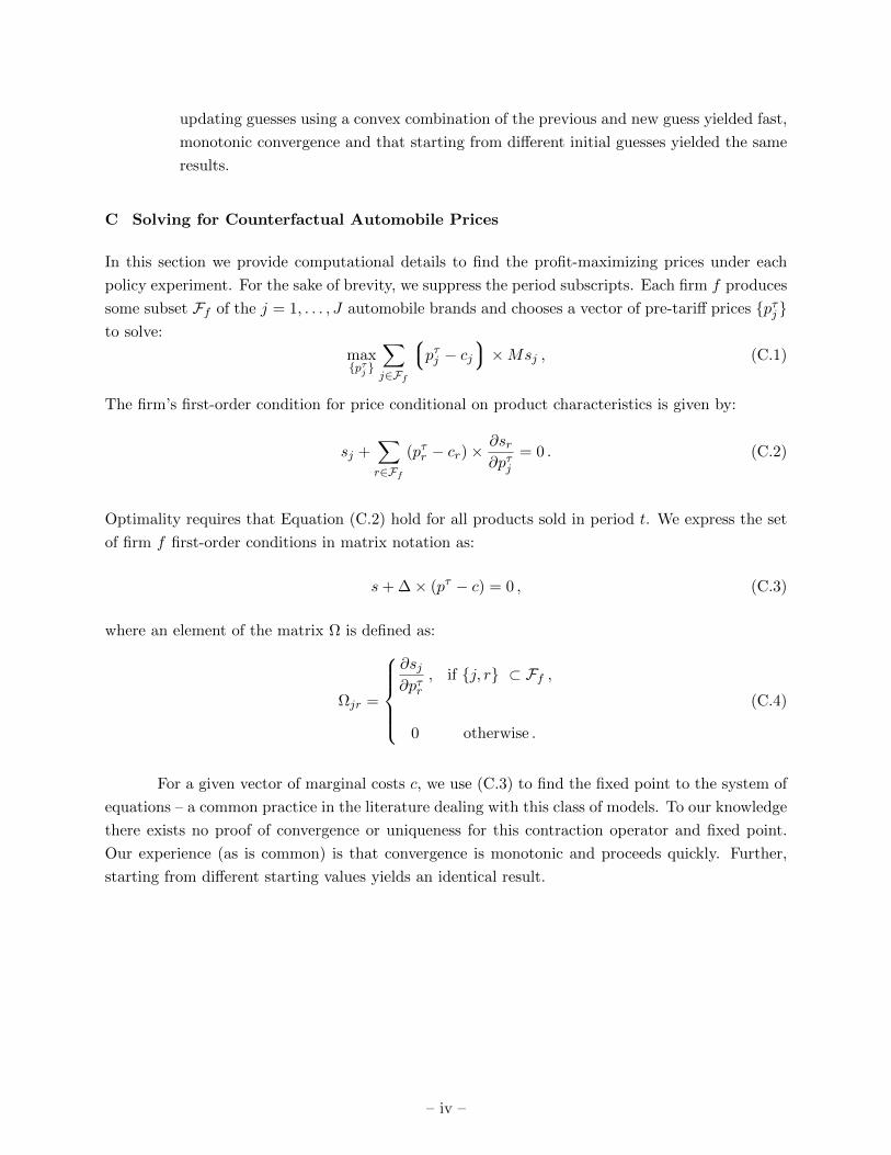
updating guesses using a convex combination of the previous and new guess yielded fast,

monotonic convergence and that starting from different initial guesses yielded the same

results.

C Solving for Counterfactual Automobile Prices

In this section we provide computational details to find the profit-maximizing prices under each

policy experiment. For the sake of brevity, we suppress the period subscripts. Each firm f produces

some subset Ff of the j = 1, . . . , J automobile brands and chooses a vector of pre-tariff prices pτj to solve:

maxpτj

∑j∈Ff

pτj − cj×Msj , (C.1)

The firm’s first-order condition for price conditional on product characteristics is given by:

sj +∑r∈Ff

(pτr − cr)×∂sr∂pτj

= 0 . (C.2)

Optimality requires that Equation (C.2) hold for all products sold in period t. We express the set

of firm f first-order conditions in matrix notation as:

s+ ∆× (pτ − c) = 0 , (C.3)

where an element of the matrix Ω is defined as:

Ωjr =

∂sj∂pτr

, if j, r ⊂ Ff ,

0 otherwise .

(C.4)

For a given vector of marginal costs c, we use (C.3) to find the fixed point to the system of

equations – a common practice in the literature dealing with this class of models. To our knowledge

there exists no proof of convergence or uniqueness for this contraction operator and fixed point.

Our experience (as is common) is that convergence is monotonic and proceeds quickly. Further,

starting from different starting values yields an identical result.

– iv –

D Additional Results

Figure D.1: Sales by Firm and Type of Engine

0 25000 50000 75000 100000 125000 150000

SKODACHRYSLER

SAABSUZUKI

HYUNDAIMITSUBISMAZDATOYOTAHONDAVOLVO

ALFA ROMROVERLANCIANISSANBMWAUDI

MERCEDESVOLKSWAGEN

FIATOPELSEATFORD

RENAULTPEUGEOTCITROEN

Diesel Gasoline

(a) Year 1992

0 25000 50000 75000 100000 125000 150000

DAEWOOSUZUKI

MITSUBISHONDA

KIAMAZDALANCIA

CHRYSLERSAAB

VOLVOTOYOTAHYUNDAIALFA ROM

ROVERSKODA

MERCEDESBMWFIAT

NISSANAUDI

VOLKSWAGENFORDOPEL

PEUGEOTRENAULT

SEATCITROEN

Diesel Gasoline

(b) Year 2000

– v –

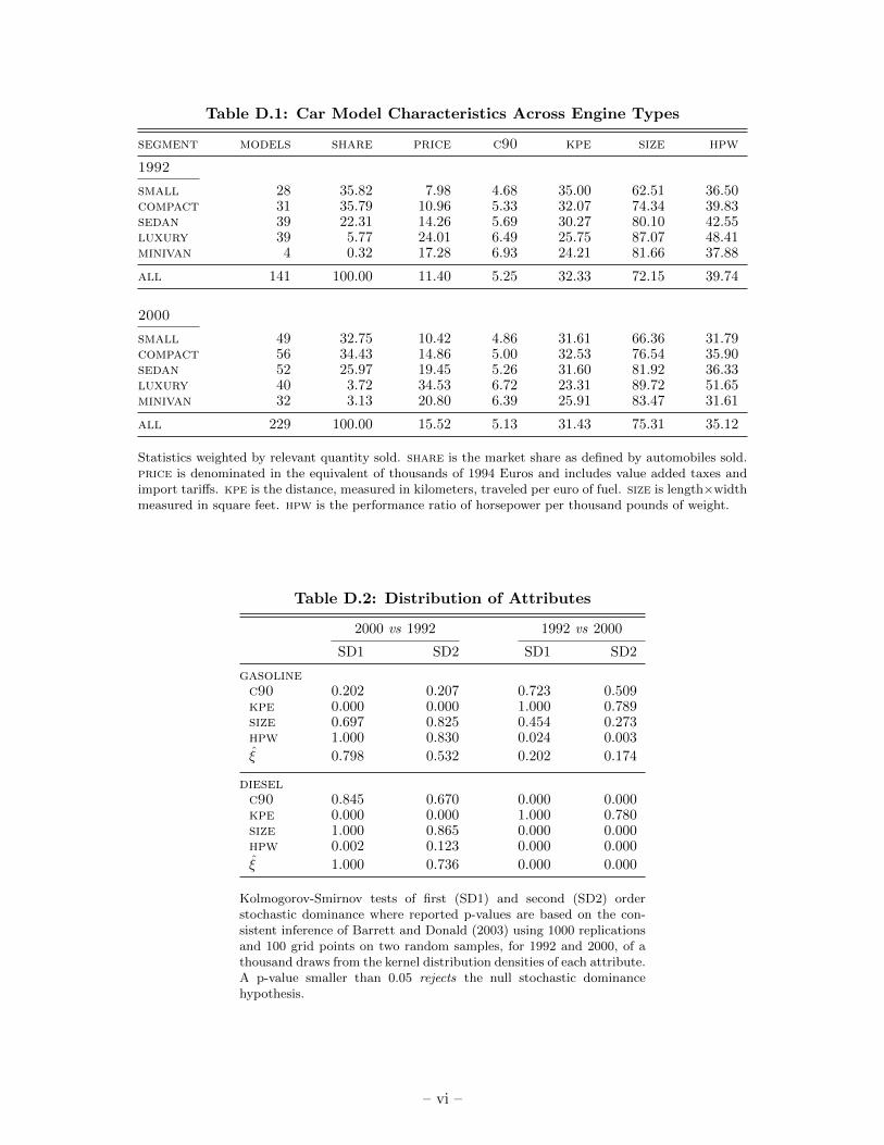
Table D.1: Car Model Characteristics Across Engine Types

segment models share price c90 kpe size hpw

1992

small 28 35.82 7.98 4.68 35.00 62.51 36.50compact 31 35.79 10.96 5.33 32.07 74.34 39.83sedan 39 22.31 14.26 5.69 30.27 80.10 42.55luxury 39 5.77 24.01 6.49 25.75 87.07 48.41minivan 4 0.32 17.28 6.93 24.21 81.66 37.88

all 141 100.00 11.40 5.25 32.33 72.15 39.74

2000

small 49 32.75 10.42 4.86 31.61 66.36 31.79compact 56 34.43 14.86 5.00 32.53 76.54 35.90sedan 52 25.97 19.45 5.26 31.60 81.92 36.33luxury 40 3.72 34.53 6.72 23.31 89.72 51.65minivan 32 3.13 20.80 6.39 25.91 83.47 31.61

all 229 100.00 15.52 5.13 31.43 75.31 35.12

Statistics weighted by relevant quantity sold. share is the market share as defined by automobiles sold.price is denominated in the equivalent of thousands of 1994 Euros and includes value added taxes andimport tariffs. kpe is the distance, measured in kilometers, traveled per euro of fuel. size is length×widthmeasured in square feet. hpw is the performance ratio of horsepower per thousand pounds of weight.

Table D.2: Distribution of Attributes

2000 vs 1992 1992 vs 2000

SD1 SD2 SD1 SD2

gasolinec90 0.202 0.207 0.723 0.509kpe 0.000 0.000 1.000 0.789size 0.697 0.825 0.454 0.273hpw 1.000 0.830 0.024 0.003

ξ 0.798 0.532 0.202 0.174

dieselc90 0.845 0.670 0.000 0.000kpe 0.000 0.000 1.000 0.780size 1.000 0.865 0.000 0.000hpw 0.002 0.123 0.000 0.000

ξ 1.000 0.736 0.000 0.000

Kolmogorov-Smirnov tests of first (SD1) and second (SD2) orderstochastic dominance where reported p-values are based on the con-sistent inference of Barrett and Donald (2003) using 1000 replicationsand 100 grid points on two random samples, for 1992 and 2000, of athousand draws from the kernel distribution densities of each attribute.A p-value smaller than 0.05 rejects the null stochastic dominancehypothesis.

– vi –

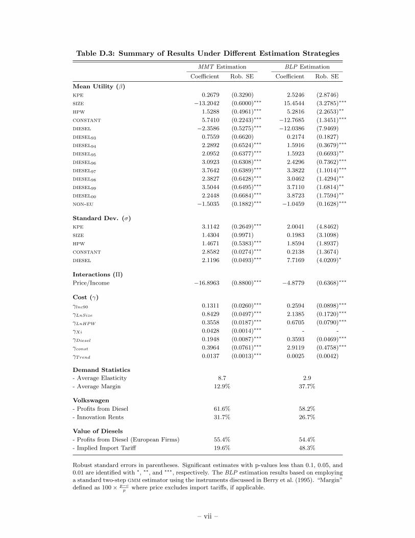
Table D.3: Summary of Results Under Different Estimation Strategies

MMT Estimation BLP Estimation

Coefficient Rob. SE Coefficient Rob. SE

Mean Utility (β)

kpe 0.2679 (0.3290) 2.5246 (2.8746)

size −13.2042 (0.6000)∗∗∗ 15.4544 (3.2785)∗∗∗

hpw 1.5288 (0.4961)∗∗∗ 5.2816 (2.2653)∗∗

constant 5.7410 (0.2243)∗∗∗ −12.7685 (1.3451)∗∗∗

diesel −2.3586 (0.5275)∗∗∗ −12.0386 (7.9469)

diesel93 0.7559 (0.6620) 0.2174 (0.1827)

diesel94 2.2892 (0.6524)∗∗∗ 1.5916 (0.3679)∗∗∗

diesel95 2.0952 (0.6377)∗∗∗ 1.5923 (0.6693)∗∗

diesel96 3.0923 (0.6308)∗∗∗ 2.4296 (0.7362)∗∗∗

diesel97 3.7642 (0.6389)∗∗∗ 3.3822 (1.1014)∗∗∗

diesel98 2.3827 (0.6428)∗∗∗ 3.0462 (1.4294)∗∗

diesel99 3.5044 (0.6495)∗∗∗ 3.7110 (1.6814)∗∗

diesel00 2.2448 (0.6684)∗∗∗ 3.8723 (1.7594)∗∗

non-eu −1.5035 (0.1882)∗∗∗ −1.0459 (0.1628)∗∗∗

Standard Dev. (σ)

kpe 3.1142 (0.2649)∗∗∗ 2.0041 (4.8462)

size 1.4304 (0.9971) 0.1983 (3.1098)

hpw 1.4671 (0.5383)∗∗∗ 1.8594 (1.8937)

constant 2.8582 (0.0274)∗∗∗ 0.2138 (1.3674)

diesel 2.1196 (0.0493)∗∗∗ 7.7169 (4.0209)∗

Interactions (Π)

Price/Income −16.8963 (0.8800)∗∗∗ −4.8779 (0.6368)∗∗∗

Cost (γ)

γlnc90 0.1311 (0.0260)∗∗∗ 0.2594 (0.0898)∗∗∗

γLnSize 0.8429 (0.0497)∗∗∗ 2.1385 (0.1720)∗∗∗

γLnHPW 0.3558 (0.0187)∗∗∗ 0.6705 (0.0790)∗∗∗

γXi 0.0428 (0.0014)∗∗∗ - -

γDiesel 0.1948 (0.0087)∗∗∗ 0.3593 (0.0469)∗∗∗

γconst 0.3964 (0.0761)∗∗∗ 2.9119 (0.4758)∗∗∗

γTrend 0.0137 (0.0013)∗∗∗ 0.0025 (0.0042)

Demand Statistics

- Average Elasticity 8.7 2.9

- Average Margin 12.9% 37.7%

Volkswagen

- Profits from Diesel 61.6% 58.2%

- Innovation Rents 31.7% 26.7%

Value of Diesels

- Profits from Diesel (European Firms) 55.4% 54.4%

- Implied Import Tariff 19.6% 48.3%

Robust standard errors in parentheses. Significant estimates with p-values less than 0.1, 0.05, and0.01 are identified with ∗, ∗∗, and ∗∗∗, respectively. The BLP estimation results based on employinga standard two-step gmm estimator using the instruments discussed in Berry et al. (1995). “Margin”defined as 100 × p−c

pwhere price excludes import tariffs, if applicable.

– vii –

Table D.4: Value of Diesels to Different Firms

Number of PricesModels Offered without Diesel Quantity Sold Profit

Year Base CF ∆ e %∆ Base CF Base CF

1992bmw 5 3 56.7 0.2 19.8 21.8 43.1 48.0fiat 20 14 30.7 0.3 58.5 57.5 76.9 74.9ford 10 6 45.7 0.3 148.8 146.0 208.7 207.6gm 14 9 53.7 0.3 122.9 124.6 181.2 188.2mercedes 7 4 22.7 0.1 13.5 12.5 39.0 35.4non-eu 25 24 44.4 0.3 38.3 43.4 55.6 65.2psa 17 9 -15.3 -0.1 202.6 148.5 311.3 205.9renault 12 8 34.9 0.3 175.4 164.8 261.0 246.4rover 7 5 31.9 0.2 15.7 17.1 21.7 24.0volkswagen 24 15 45.2 0.3 173.0 171.8 273.1 276.0

2000bmw 7 4 0.1 0.0 29.5 25.2 88.2 79.6fiat 27 14 60.5 0.5 59.8 51.5 97.9 83.7ford 17 10 60.9 0.4 123.2 97.2 230.6 189.4gm 15 9 53.0 0.4 146.2 105.7 269.1 203.5mercedes 12 6 9.8 0.1 24.6 24.9 71.0 73.4non-eu 70 50 56.4 0.4 160.6 187.4 254.9 307.8psa 19 9 -5.7 0.0 306.0 158.5 608.5 299.2renault 11 6 53.6 0.4 176.3 117.4 309.4 219.2rover 9 5 60.7 0.4 18.7 16.7 37.4 33.9volkswagen 42 21 27.0 0.3 319.8 199.8 679.1 432.3

“Base” refers to benchmark equilibrium in the data while “CF” refers to the equilibrium without diesels cars. Under“Prices without Diesel”, ∆e refers to the average price change (in 1994 Euros) while %∆ refers to the averagepercentage price change. “Quantity Sold” is the number of new car sales (in thousands). “Profit” measured inmillions of 1994 Euros.

– viii –