abstract 1. introduction · for esbas upper bounds of the pseudo-regrets deﬁned in section 3...

Algorithm selection of off-policy reinforcement learning algorithms

Romain Laroche [email protected] done at: Orange Labs, 44 Avenue de la République, Châtillon, FranceNow at: Maluuba, 2000 Peel Street, Montréal, Canada

Raphaël Féraud [email protected]

Orange Labs, 2 Avenue Pierre Marzin, Lannion, France

Abstract

Dialogue systems rely on a careful reinforcementlearning design: the learning algorithm and itsstate space representation. In lack of more rigor-ous knowledge, the designer resorts to its practicalexperience to choose the best option. In order toautomate and to improve the performance of theaforementioned process, this article formalisesthe problem of online off-policy reinforcementlearning algorithm selection. A meta-algorithmis given for input a portfolio constituted of sev-eral off-policy reinforcement learning algorithms.It then determines at the beginning of each newtrajectory, which algorithm in the portfolio is incontrol of the behaviour during the full next trajec-tory, in order to maximise the return. The articlepresents a novel meta-algorithm, called EpochalStochastic Bandit Algorithm Selection (ESBAS).Its principle is to freeze the policy updates at eachepoch, and to leave a rebooted stochastic ban-dit in charge of the algorithm selection. Undersome assumptions, a thorough theoretical analy-sis demonstrates its near-optimality consideringthe structural sampling budget limitations. Then,ESBAS is put to the test in a set of experimentswith various portfolios, on a negotiation dialoguegame. The results show the practical benefits ofthe algorithm selection for dialogue systems, inmost cases even outperforming the best algorithmin the portfolio, even when the aforementionedassumptions are transgressed.

Shorter version under review by the International Conference onMachine Learning (ICML).

1. IntroductionReinforcement Learning (RL) (Sutton & Barto, 1998) isa machine learning framework intending to optimise thebehaviour of an agent interacting with an unknown environ-ment. For the most practical problems, trajectory collectionis costly and sample efficiency is the main key performanceindicator. This is for instance the case for dialogue sys-tems (Singh et al., 1999) and robotics (Brys et al., 2015). Asa consequence, when applying RL to a new problem, onemust carefully choose in advance a model, an optimisationtechnique, and their parameters in order to learn an adequatebehaviour given the limited sample set at hand.

In particular, for 20 years, research has developed andapplied RL algorithms for Spoken Dialogue Systems, in-volving a large range of dialogue models and algorithmsto optimise them. Just to cite a few algorithms: MonteCarlo (Levin & Pieraccini, 1997),Q-Learning (Walker et al.,1998), SARSA (Frampton & Lemon, 2006), MVDP algo-rithms (Laroche et al., 2009), Kalman Temporal Differ-ence (Pietquin et al., 2011), Fitted-Q Iteration (Genevay& Laroche, 2016), Gaussian Process RL (Gašic et al., 2010),and more recently Deep RL (Fatemi et al., 2016). Addition-ally, most of them require the setting of hyper parametersand a state space representation. When applying these re-search results to a new problem, these choices may dramati-cally affect the speed of convergence and therefore, the dia-logue system performance. Facing the complexity of choice,RL and dialogue expertise is not sufficient. Confronted tothe cost of data, the popular trial and error approach showsits limits.

Algorithm selection (Rice, 1976; Smith-Miles, 2009; Kot-thoff, 2012) is a framework for comparing several algo-rithms on a given problem instance. The algorithms aretested on several problem instances, and hopefully, the al-gorithm selection learns from those experiences which al-gorithm should be the most efficient given a new probleminstance. In our setting, only one problem instance is consid-ered, but several experiments are led to determine the fittest

arX

iv:1

701.

0881

0v1

[st

at.M

L]

30

Jan

2017


algorithm to deal with it.

Thus, we developed an online learning version (Gagliolo &Schmidhuber, 2006; 2010) of algorithm selection. It consistsin testing several algorithms on the task and in selecting thebest one at a given time. Indeed, it is important to noticethat, as new data is collected, the algorithms improve theirperformance and that an algorithm might be the worst at ashort-term horizon, but the best at a longer-term horizon. Inorder to avoid confusion, throughout the whole article, thealgorithm selector is called a meta-algorithm, and the set ofalgorithms available to the meta-algorithm is called a port-folio. Defined as an online learning problem, our algorithmselection task has for objective to minimise the expectedregret.

At each online algorithm selection, only the selected algo-rithm is experienced. Since the algorithms learn from theirexperience, it implies a requirement for a fair budget alloca-tion between the algorithms, so that they can be equitablyevaluated and compared. Budget fairness is in direct con-tradiction with the expected regret minimisation objective.In order to circumvent this, the reinforcement algorithmsin the portfolio are assumed to be off-policy, meaning thatthey can learn from experiences generated from an arbitrarynon-stationary behavioural policy. Section 2 provides a uni-fying view of reinforcement learning algorithms, that allowsinformation sharing between all algorithms of the portfolio,whatever their decision processes, their state representations,and their optimisation techniques.

Then, Section 3 formalises the problem of online selectionof off-policy reinforcement learning algorithms. It intro-duces three definitions of pseudo-regret and states threeassumptions related to experience sharing and budget fair-ness among algorithms. Beyond the sample efficiency issues,the online algorithm selection approach addresses further-more four distinct practical problems for spoken dialoguesystems and online RL-based systems more generally. First,it enables a systematic benchmark of models and algorithmsfor a better understanding of their strengths and weaknesses.Second, it improves robustness against implementation bugs:if an algorithm fails to terminate, or converges to an aber-rant policy, it will be dismissed and others will be selectedinstead. Third, convergence guarantees and empirical effi-ciency may be united by covering the empirically efficientalgorithms with slower algorithms that have convergenceguarantees. Fourth and last, it enables staggered learning:shallow models converge the fastest and consequently con-trol the policy in the early stages, while deep models dis-cover the best solution later and control the policy in latestages.

Afterwards, Section 4 presents the Epochal Stochastic Ban-dit Algorithm Selection (ESBAS), a novel meta-algorithmaddressing the online off-policy reinforcement learning al-

gorithm selection problem. Its principle is to divide thetime-scale into epochs of exponential length inside whichthe algorithms are not allowed to update their policies. Dur-ing each epoch, the algorithms have therefore a constantpolicy and a stochastic multi-armed bandit can be in chargeof the algorithm selection with strong pseudo-regret theo-retical guaranties. A thorough theoretical analysis providesfor ESBAS upper bounds of the pseudo-regrets defined inSection 3 under the assumptions stated in the same section.

Next, Section 5 experiments ESBAS on a simulated dialoguetask, and presents the experimental results, which demon-strate the practical benefits of ESBAS: in most cases outper-forming the best algorithm in the portfolio, even though itsprimary goal was just to be almost as good as it.

Finally, Sections 6 and 7 conclude the article with respec-tively related works and prospective ideas of improvement.

2. Unifying view of reinforcement learningalgorithms

The goal of this section is to enable information sharingbetween algorithms, even though they are considered asblack boxes. We propose to share their trajectories expressedin a universal format: the interaction process.

Reinforcement Learning (RL) consists in learning throughtrial and error to control an agent behaviour in a stochasticenvironment. More formally, at each time step t ∈ N, theagent performs an action a(t) ∈ A, and then perceives fromits environment a signal o(t) ∈ Ω called observation, andreceives a reward R(t) ∈ R. Figure 1 illustrates the RLframework. This interaction process is not Markovian: theagent may have an internal memory.

In this article, the reward function is assumed to be boundedbetween Rmin and Rmax, and we define the RL problemas episodic. Let us introduce two time scales with differentnotations. First, let us define meta-time as the time scalefor algorithm selection: at one meta-time τ corresponds ameta-algorithm decision, i.e. the choice of an algorithm and

Agent

Stochasticenvironment

a(t)o(t+ 1) R(t+ 1)

Figure 1. Reinforcement Learning framework: after performingaction a(t), the agent perceives observation o(t+ 1) and receivesreward R(t+ 1) from the environment.


the generation of a full episode controlled with the policydetermined by the chosen algorithm. Its realisation is calleda trajectory. Second, RL-time is defined as the time scaleinside a trajectory, at one RL-time t corresponds one tripletcomposed of an observation, an action, and a reward.

Let E denote the space of trajectories. A trajectory ετ ∈E

collected at meta-time τ is formalised as a sequence of(observation, action, reward) triplets:

ετ = 〈oτ (t), aτ (t), Rτ (t)〉t∈J1,|ετ |K ∈E, (2.1)

where |ετ | is the length of trajectory ετ . The objective is,given a discount factor 0 ≤ γ < 1, to generate trajectorieswith high discounted cumulative reward, also called return,and noted µ(ετ ):

µ(ετ ) =

|ετ |∑t=1

γt−1Rτ (t). (2.2)

Since γ < 1 and Rmin ≤ R ≤ Rmax, the return isbounded:

Rmin

1− γ≤ µ(ετ ) ≤

Rmax

1− γ. (2.3)

The trajectory set at meta-time T is denoted by:

DT = εττ∈J1,T K ∈ET . (2.4)

A sub-trajectory of ετ until RL-time t is called the historyat RL-time t and written ετ (t) with t ≤ |ετ |. The historyrecords what happened in episode ετ until RL-time t:

ετ (t) = 〈oτ (t′), aτ (t′), Rτ (t′)〉t′∈J1,tK ∈E. (2.5)

The goal of each reinforcement learning algorithm α is tofind a policy π∗ : E → A which yields optimal expectedreturns. Such an algorithm α is viewed as a black box thattakes as an input a trajectory set D ∈ E+, where E+ isthe ensemble of trajectory sets of undetermined size: E+ =⋃T∈NE

T , and that outputs a policy παD. Consequently, areinforcement learning algorithm is formalised as follows:

α : E+ → (E → A). (2.6)

Such a high level definition of the RL algorithms allowsto share trajectories between algorithms: a trajectory asa sequence of observations, actions, and rewards can beinterpreted by any algorithm in its own decision process andstate representation.

For instance, RL algorithms classically rely on an MDPdefined on a state space representation SαD thanks to a pro-jection ΦαD:

ΦαD : E → SαD. (2.7)

The state representation may be built dynamically as thetrajectories are collected. Many algorithms doing so canbe found in the literature, for instance (Legenstein et al.,2010; Böhmer et al., 2015; El Asri et al., 2016; Williamset al., 2016). Then, α may learn its policy παDT from thetrajectories projected on its state space representation andsaved as a transition set: a transition is defined as a quadru-plet 〈sτ (t), aτ (t), Rτ (t), sτ (t+ 1)〉, with state sτ (t) ∈ SαD,action aτ (t) ∈ A, reward Rτ (t) ∈ R, and next statesτ (t+1) ∈ SαD. Off-policy reinforcement learning optimisa-tion techniques compatible with this approach are numerousin the literature (Maei et al., 2010): Q-Learning (Watkins,1989), Fitted-Q Iteration (Ernst et al., 2005), Kalman Tem-poral Difference (Geist & Pietquin, 2010), etc.

Another option would be to perform end-to-end reinforce-ment learning (Riedmiller, 2005; Mnih et al., 2013; Silveret al., 2016). As well, any post-treatment of the state set, anyalternative decision process model, such as POMDPs (Love-joy, 1991; Azizzadenesheli et al., 2016), and any off-policytechnique for control optimisation may be used. The algo-rithms are defined here as black boxes and the consideredmeta-algorithms will be indifferent to how the algorithmscompute their policies, granted they satisfy the assumptionsmade in the following section.

3. Algorithm selection model3.1. Batch algorithm selection

Algorithm selection (Rice, 1976) for combinatorialsearch (Kotthoff, 2012) consists in deciding which experi-ments should be carried out, given a problem instance and afixed amount of computational resources: generally speak-ing computer-time, memory resources, time and/or money.Algorithms are considered efficient if they consume littleresource. This approach, often compared and applied to ascheduling problem (Gomes & Selman, 2001), experienceda lot of success for instance in the SAT competition (Xuet al., 2008).

Algorithm selection applied to machine learning, also calledmeta-learning, is mostly dedicated to error minimisationgiven a corpus of limited size. Indeed, these algorithms donot deliver in fine the same answer. In practice, algorithmselection can be applied to arbitrary performance metricsand modelled in the same framework. In the classical batchsetting, the notations of the machine learning algorithmselection problem are described in (Smith-Miles, 2009) asfollows:

• I is the space of problem instances;

• P is the portfolio, i.e. the collection of available algo-rithms;


• µ : I × P → R is the objective function, i.e. a perfor-mance metrics enabling to rate an algorithm on a giveninstance;

• Ψ : I → Rk are the features characterising the proper-ties of problem instances.

The principle consists in collecting problem instances andin solving them with the algorithms in the portfolio P . Themeasures µ provide evaluations of the algorithms on thoseinstances. Then, the aggregation of their features Ψ withthe measures µ constitutes a training set. Finally, any super-vised learning techniques can be used to learn an optimisedmapping between the instances and the algorithms.

3.2. Online algorithm selection

Nevertheless, in our case, I is not large enough to learn anefficient model, it might even be a singleton. Consequently,it is not possible to regress a general knowledge from aparametrisation Ψ. This is the reason why the online learn-ing approach is tackled in this article: different algorithmsare experienced and evaluated during the data collection.Since it boils down to a classical exploration/exploitationtrade-off, multi-armed bandit (Bubeck & Cesa-Bianchi,2012) have been used for combinatorial search algorithmselection (Gagliolo & Schmidhuber, 2006; 2010) and evolu-tionary algorithm meta-learning (Fialho et al., 2010).

In the online setting, the algorithm selection problem foroff-policy reinforcement learning is new and we define it asfollows:

• D ∈E+ is the trajectory set;

• P = αkk∈J1,KK is the portfolio;

• µ : E → R is the objective function defined in Equa-tion 2.2.

Pseudo-code 1 formalises the online algorithm selectionsetting. A meta-algorithm is defined as a function from atrajectory set to the selection of an algorithm:

σ : E+ → P. (3.1)

The meta-algorithm is queried at each meta-time τ =|Dτ−1|+1, with input Dτ−1, and it ouputs algorithmσ (Dτ−1) = σ(τ) ∈ P controlling with its policy πσ(τ)

Dτ−1

the generation of the trajectory εσ(τ)τ in the stochastic envi-

ronment. Let EµαD be a condensed notation for the expectedreturn of policy παD that was learnt from trajectory set D byalgorithm α:

EµαD = EπαD [µ (ε)] . (3.2)

Pseudo-code 1 Online algorithm selection settingData: P ← αkk∈J1,KK: algorithm portfolioData: D0 ← ∅: trajectory setfor τ ← 1 to∞ do

Select σ (Dτ−1) = σ(τ) ∈ P;Generate trajectory ετ with policy πσ(τ)

Dτ−1;

Get return µ(ετ );Dτ ← Dτ−1 ∪ ετ;

end

The final goal is to optimise the cumulative expected return.It is the expectation of the sum of rewards obtained after arun of T trajectories:

Eσ

[T∑τ=1

µ(εσ(τ)τ

)]=

T∑τ=1

∑D∈Eτ−1

P(D|σ)Eµσ(τ)D ,

(3.3a)

(3.3b)Eσ

[T∑τ=1

µ(εσ(τ)τ

)]=

T∑τ=1

Eσ[Eµσ(τ)Dστ−1

],

(3.3c)Eσ

[T∑τ=1

µ(εσ(τ)τ

)]= Eσ

[T∑τ=1

Eµσ(τ)Dστ−1

].

Equations 3.3a, 3.3b and 3.3c transform the cumulativeexpected return into two nested expectations. The outsideexpectation Eσ assumes the algorithm selection fixed andaverages over the trajectory set stochastic collection and thecorresponding algorithms policies, which may also rely ona stochastic process. The inside expectation Eµ assumes thepolicy fixed and averages the evaluation over its possibletrajectories in the stochastic environment. Equation 3.3atransforms the expectation into its probabilistic equivalent,P(D|σ) denoting the probability density of generating trajec-tory set D conditionally to the meta-algorithm σ. Equation3.3b transforms back the probability into a local expectation,and finally Equation 3.3c simply applies the commutativitybetween the sum and the expectation.

Nota bene: there are three levels of decision: meta-algorithmσ selects an algorithm α that computes a policy π that inturn controls the actions. We focus in this paper on themeta-algorithm level.

3.3. Meta-algorithm evaluation

In order to evaluate the meta-algorithms, let us formulatetwo additional notations. First, the optimal expected returnEµ∗∞ is defined as the highest expected return achievable


by a policy of an algorithm in portfolio P: ∀D ∈E+, ∀α ∈ P, EµαD ≤ Eµ∗∞,

∀ε > 0, ∃D ∈E+, ∃α ∈ P, Eµ∗∞ − EµαD < ε.

(3.4)

Second, for every algorithm α in the portfolio, let us defineσα as its canonical meta-algorithm, i.e. the meta-algorithmthat always selects algorithm α: ∀τ , σα(τ) = α.

The absolute pseudo-regret ρσabs(T ) defines the regret as theloss for not having controlled the trajectory with an optimalpolicy.Definition 1 (Absolute pseudo-regret). The absolutepseudo-regret ρσabs(T ) compares the meta-algorithm’s ex-pected return with the optimal expected return:

ρσabs(T ) = TEµ∗∞ − Eσ

[T∑τ=1

Eµσ(τ)Dστ−1

]. (3.5)

The absolute pseudo-regret ρσabs(T ) is a well-foundedpseudo-regret definition. However, it is worth noting that anoptimal meta-algorithm will not yield a null regret becausea large part of the absolute pseudo-regret is caused by thesub-optimality of the algorithm policies when the trajectoryset is still of limited size. Indeed, the absolute pseudo-regretconsiders the regret for not selecting an optimal policy: ittakes into account both the pseudo-regret of not selectingthe best algorithm and the pseudo-regret of the algorithmsfor not finding an optimal policy. Since the meta-algorithmdoes not interfere with the training of policies, it cannotaccount for the pseudo-regret related to the latter.

In order to have a pseudo-regret that is relative to the learn-ing ability of the best algorithm and that better accounts forthe efficiency of the algorithm selection task, we introducethe notion of relative pseudo-regret.Definition 2 (Relative pseudo-regret). The relative pseudo-regret ρσrel(T ) compares the σ meta-algorithm’s expectedreturn with the expected return of the best canonical meta-algorithm:

ρσrel(T ) = maxα∈P

Eσα[T∑τ=1

EµαDσατ−1

]− Eσ

[T∑τ=1

Eµσ(τ)Dστ−1

].

(3.6)

It is direct from Equations 3.5 and 3.6 that the relativepseudo-regret can be expressed in function of absolutepseudo-regrets of the meta-algorithm σ and the canonicalmeta-algorithms σα:

ρσrel(T ) = ρσabs(T )−maxα∈P

ρσα

abs(T ). (3.7)

Since one shallow algorithm might be faster in early stagesand a deeper one more effective later, a good meta-algorithm

may achieve a negative relative pseudo-regret, which isill-defined as a pseudo-regret definition. Still, the relativepseudo-regret ρσrel(T ) is useful as an empirical evaluationmetric. A large relative pseudo-regret shows that the meta-algorithm failed to consistently select the best algorithm(s)in the portfolio. A small, null, or even negative relativepseudo-regret demonstrates that using a meta-algorithm is aguarantee for selecting the algorithm that is the most adaptedto the problem.

3.4. Assumptions

The theoretical analysis is hindered by the fact that algo-rithm selection, not only directly influences the return distri-bution, but also the trajectory set distribution and thereforethe policies learnt by algorithms for next trajectories, whichwill indirectly affect the future expected returns. In orderto allow policy comparison, based on relation on trajectorysets they are derived from, our analysis relies on three as-sumptions whose legitimacy is discussed in this section andfurther developed under the practical aspects in Section 5.7.

Assumption 1 (More data is better data). The algorithmsproduce better policies with a larger trajectory set on aver-age, whatever the algorithm that controlled the additionaltrajectory:

∀D ∈E+, ∀α, α′ ∈ P , EµαD ≤ Eα′[EµαD∪εα′

]. (3.8)

Assumption 1 states that algorithms are off-policy learnersand that additional data cannot lead to performance degrada-tion on average. An algorithm that is not off-policy could bebiased by a specific behavioural policy and would thereforetransgress this assumption.

Assumption 2 (Order compatibility). If an algorithm pro-duces a better policy with one trajectory set than with an-other, then it remains the same, on average, after collectingan additional trajectory from any algorithm:

∀D,D′ ∈E+, ∀α, α′ ∈ P ,

EµαD < EµαD′ ⇒ Eα′[EµαD∪εα′

]≤ Eα′

[EµαD′∪εα′

].

(3.9)

Assumption 2 states that a performance relation betweentwo policies learnt by a given algorithm from two trajectorysets is preserved on average after adding another trajectory,whatever the behavioural policy used to generate it.

From these two assumptions, Theorem 1 provides an up-per bound in order of magnitude in function of the worstalgorithm in the portfolio. It is verified for any algorithmselection σ:


Theorem 1 (Not worse than the worst). The absolutepseudo-regret is bounded by the worst algorithm absolutepseudo-regret in order of magnitude:

∀σ, ρσabs(T ) ∈ O(

maxα∈P

ρσα

abs(T )

). (3.10)

Proof. See the appendix.

Contrarily to what the name of Theorem 1 suggests, a meta-algorithm might be worse than the worst algorithm (sim-ilarly, it can be better than the best algorithm), but not inorder of magnitude. Its proof is rather complex for suchan intuitive and loose result because, in order to control allthe possible outcomes, one needs to translate the selectionsof algorithm α with meta-algorithm σ into the canonicalmeta-algorithm σα’s view, in order to be comparable withit. This translation is not obvious when the meta-algorithmσ and the algorithms it selects act tricky. See the proof foran example.

The fairness of budget distribution has been formalised in(Cauwet et al., 2015). It is the property stating that everyalgorithm in the portfolio has as much resources as the oth-ers, in terms of computational time and data. It is an issuein most online algorithm selection problems, since the algo-rithm that has been the most selected has the most data, andtherefore must be the most advanced one. A way to circum-vent this issue is to select them equally, but, in an onlinesetting, the goal of algorithm selection is precisely to selectthe best algorithm as often as possible. In short, explorationand evaluation require to be fair and exploitation implies tobe unfair. Our answer is to require that all algorithms in theportfolio are learning off-policy, i.e. without bias inducedby the behavioural policy used in the learning dataset.

By assuming that all algorithms learn off-policy, we allowinformation sharing (Cauwet et al., 2015) between algo-rithms. They share the trajectories they generate. As a con-sequence, we can assume that every algorithm, the least orthe most selected ones, will learn from the same trajectoryset. Therefore, the control unbalance does not directly leadto unfairness in algorithms performances: all algorithmslearn equally from all trajectories.

However, unbalance might still remain in the explorationstrategy if, for instance, an algorithm takes more benefitfrom the exploration it has chosen than the one chosen byanother algorithm. In this article, we speculate that thischosen-exploration effect is negligible. More formally, inthis article, for analysis purposes, the algorithm selectionis assumed to be absolutely fair regardless the explorationunfairness we just discussed about. This is expressed byAssumption 3.

Assumption 3 (Learning is fair). If one trajectory set isbetter than another for one given algorithm, it is the samefor other algorithms.

∀α, α′ ∈ P, ∀D,D′ ∈E+,

EµαD < EµαD′ ⇒ Eµα′D ≤ Eµα′D′ .(3.11)

In practical problems, Assumptions 2 and 3 are defeated, butempirical results in Section 5 demonstrate that the ESBASalgorithm presented in Section 4 is robust to the assumptiontransgressions.

4. Epochal stochastic bandit algorithmselection

An intuitive way to solve the algorithm selection problemis to consider algorithms as arms in a multi-armed banditsetting. The bandit meta-algorithm selects the algorithm con-trolling the next trajectory ε and the trajectory return µ(ε)constitutes the reward of the bandit. However, a stochasticbandit cannot be directly used because the algorithms perfor-mances vary and improve with time (Garivier & Moulines,2008). Adversarial multi-arm bandits are designed for non-stationary environments (Auer et al., 2002b; Allesiardo &Féraud, 2015), but the exploitation the structure of our algo-rithm selection problem makes it possible to obtain pseudo-regrets of order of magnitude lower than Ω(

√T ).

Alternatively, one might consider using policy search meth-ods (Ng & Jordan, 2000), but they rely on a state space rep-resentation in order to apply the policy gradient. And in ourcase, neither policies do share any, nor the meta-algorithmdoes have at disposal any other than the intractable historiesετ (t) defined in Equation 2.5.

4.1. ESBAS description

To solve the off-policy RL algorithm selection problem, wepropose a novel meta-algorithm called Epochal StochasticBandit Algorithm Selection (ESBAS). Because of the non-stationarity induced by the algorithm learning, the stochas-tic bandit cannot directly select algorithms. Instead, thestochastic bandit can choose fixed policies. To comply tothis constraint, the meta-time scale is divided into epochsinside which the algorithms policies cannot be updated: thealgorithms optimise their policies only when epochs start, insuch a way that the policies are constant inside each epoch.As a consequence and since the returns are bounded in Equa-tion 2.3, at each new epoch, the problem can be cast into anindependent stochastic K-armed bandit Ξ, with K = |P|.

The ESBAS meta-algorithm is formally sketched in Pseudo-code 2 embedding UCB1 (Auer et al., 2002a) as the stochas-tic K-armed bandit Ξ. The meta-algorithm takes as an input


Pseudo-code 2 ESBAS with UCB1Data: P ← αkk∈J1,KK ; // Portfolio: the set of algorithms.Data: D0 ← ∅ ; // Trajectory set: initiated to ∅.for β ← 0 to∞ ; // For each epoch β,do

for αk ∈ P ; // For each algorithm α,do

πkD2β−1

: policy learnt by αk on D2β−1 ; // Update the current policy πkD2β−1

.

endn← 0, ∀αk ∈ P , nk ← 0, and xk ← 0 ; // Initialise a new UCB1 k-armed bandit.for τ ← 2β to 2β+1 − 1; // For each meta-time step τ,do

αkmax = argmaxαk∈P

xk +

√ξ

log(n)

nk

; // UCB1 bandit selects the policy.

Generate trajectory ετ with policy πkmaxD2β−1

; // This policy controls the next trajectory.

Get return µ(ετ ), Dτ ← Dτ−1 ∪ ετ; // The return is observed as the UCB1 reward.

xkmax ←nkmaxxkmax + µ(ετ )

nkmax + 1; // Update the empirical mean of selected arm.

nkmax ← nkmax + 1 and n← n+ 1; // Update the number of arm selections.end

end

the set of algorithms in the portfolio. Meta-time scale is frag-mented into epochs of exponential size. The βth epoch lasts2β meta-time steps, so that, at meta-time τ = 2β , epoch βstarts. At the beginning of each epoch, the ESBAS meta-algorithm asks each algorithm in the portfolio to updatetheir current policy. Inside an epoch, the policy is neverupdated anymore. At the beginning of each epoch, a new Ξinstance is reset and run. During the whole epoch, Ξ decidesat each meta-time step which algorithm is in control of thenext trajectory.

4.2. ESBAS short-sighted pseudo-regret analysis

It has to be noted that ESBAS simply intends to minimisethe regret for not choosing the best algorithm at a givenmeta-time τ . It is somehow short-sighted: it does not intendto optimise its algorithms learning. The following short-sighted pseudo-regret definition captures the function ES-BAS intends to minimise.Definition 3 (Short-sighted pseudo-regret). The short-sighted pseudo-regret ρσss(T ) is the difference between theimmediate best expected return algorithm and the one se-lected:

ρσss(T ) = Eσ

[T∑τ=1

(maxα∈P

EµαDστ−1− Eµσ(τ)

Dστ−1

)]. (4.1)

The short-sighted pseudo-regret optimality depends on themeta-algorithm itself. For instance, a poor deterministic

algorithm might be optimal at meta-time τ but yield no newinformation, implying the same situation at meta-time τ +1,and so on. Thus, a meta-algorithm that exclusively selectsthe deterministic algorithm would achieve a short-sightedpseudo-regret equal to 0, but selecting other algorithms are,in the long run, more efficient. Theorem 2 expresses inorder of magnitude an upper bound for the short-sightedpseudo-regret of ESBAS. But first, let define the gaps:

∆αβ = max

α′∈PEµα

′

DσESBAS

2β−1

− EµαDσESBAS

2β−1

. (4.2)

It is the difference of expected return between the best al-gorithm during epoch β and algorithm α. The smallest nonnull gap at epoch β is noted:

∆†β = minα∈P,∆α

β>0∆αβ . (4.3)

If ∆†β does not exist, i.e. if there is no non-null gap, theproblem is trivial and the regret is null. Upper bounds onshort-sighted and absolute pseudo-regrets are derived.

Theorem 2 (ESBAS short-sighted pseudo-regret). If thestochastic multi-armed bandit Ξ guarantees a regret of orderof magnitude O(log(T )/∆†β), then:

ρσESBAS

ss (T ) ∈ O

blog(T )c∑β=0

β

∆†β

. (4.4)


∆†β ρσESBAS

ss (T )

Θ (1/T ) O (log(T ))

Θ(T−c†), c† ≥ 0.5 O(T 1−c†)

Θ(T−c†), c† < 0.5 O(T c

†log(T ))

Θ (1) O(log2(T )/∆†∞

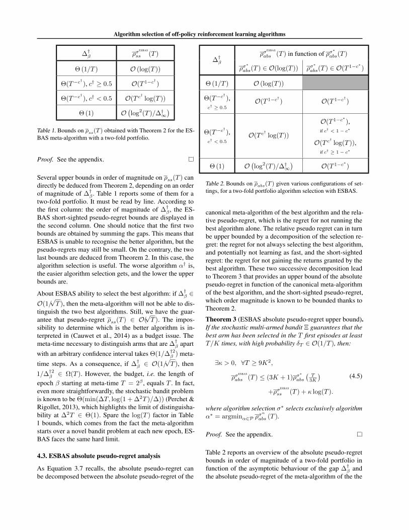
)Table 1. Bounds on ρss(T ) obtained with Theorem 2 for the ES-BAS meta-algorithm with a two-fold portfolio.


Several upper bounds in order of magnitude on ρss(T ) candirectly be deduced from Theorem 2, depending on an orderof magnitude of ∆†β . Table 1 reports some of them for atwo-fold portfolio. It must be read by line. According tothe first column: the order of magnitude of ∆†β , the ES-BAS short-sighted pseudo-regret bounds are displayed inthe second column. One should notice that the first twobounds are obtained by summing the gaps. This means thatESBAS is unable to recognise the better algorithm, but thepseudo-regrets may still be small. On the contrary, the twolast bounds are deduced from Theorem 2. In this case, thealgorithm selection is useful. The worse algorithm α† is,the easier algorithm selection gets, and the lower the upperbounds are.

About ESBAS ability to select the best algorithm: if ∆†β ∈O(1/√T ), then the meta-algorithm will not be able to dis-

tinguish the two best algorithms. Still, we have the guar-antee that pseudo-regret ρss(T ) ∈ O(

√T ). The impos-

sibility to determine which is the better algorithm is in-terpreted in (Cauwet et al., 2014) as a budget issue. Themeta-time necessary to distinguish arms that are ∆†β apartwith an arbitrary confidence interval takes Θ(1/∆†2β ) meta-

time steps. As a consequence, if ∆†β ∈ O(1/√T ), then

1/∆†2β ∈ Ω(T ). However, the budget, i.e. the length ofepoch β starting at meta-time T = 2β , equals T . In fact,even more straightforwardly, the stochastic bandit problemis known to be Θ(min(∆T, log(1 + ∆2T )/∆)) (Perchet &Rigollet, 2013), which highlights the limit of distinguisha-bility at ∆2T ∈ Θ(1). Spare the log(T ) factor in Table1 bounds, which comes from the fact the meta-algorithmstarts over a novel bandit problem at each new epoch, ES-BAS faces the same hard limit.

4.3. ESBAS absolute pseudo-regret analysis

As Equation 3.7 recalls, the absolute pseudo-regret canbe decomposed between the absolute pseudo-regret of the

∆†βρσ

ESBAS

abs (T ) in function of ρσ∗

abs(T )

ρσ∗

abs(T ) ∈ O(log(T )) ρσ∗

abs(T ) ∈ O(T 1−c∗)

Θ (1/T ) O (log(T ))

Θ(T−c†),

c† ≥ 0.5O(T 1−c†) O(T 1−c†)

Θ(T−c†),

c† < 0.5O(T c

†log(T ))

O(T 1−c∗),if c† < 1− c∗

O(T c†

log(T )),if c† ≥ 1− c∗

Θ (1) O(log2(T )/∆†∞

)O(T 1−c∗)

Table 2. Bounds on ρabs(T ) given various configurations of set-tings, for a two-fold portfolio algorithm selection with ESBAS.

canonical meta-algorithm of the best algorithm and the rela-tive pseudo-regret, which is the regret for not running thebest algorithm alone. The relative pseudo regret can in turnbe upper bounded by a decomposition of the selection re-gret: the regret for not always selecting the best algorithm,and potentially not learning as fast, and the short-sightedregret: the regret for not gaining the returns granted by thebest algorithm. These two successive decomposition leadto Theorem 3 that provides an upper bound of the absolutepseudo-regret in function of the canonical meta-algorithmof the best algorithm, and the short-sighted pseudo-regret,which order magnitude is known to be bounded thanks toTheorem 2.

Theorem 3 (ESBAS absolute pseudo-regret upper bound).If the stochastic multi-armed bandit Ξ guarantees that thebest arm has been selected in the T first episodes at leastT/K times, with high probability δT ∈ O(1/T ), then:

∃κ > 0, ∀T ≥ 9K2,

ρσESBAS

abs (T ) ≤ (3K + 1)ρσ∗

abs

(T

3K

)+ρσ

ESBAS

ss (T ) + κ log(T ).

(4.5)

where algorithm selection σ∗ selects exclusively algorithmα∗ = argminα∈P ρ

σα

abs (T ).


Table 2 reports an overview of the absolute pseudo-regretbounds in order of magnitude of a two-fold portfolio infunction of the asymptotic behaviour of the gap ∆†β andthe absolute pseudo-regret of the meta-algorithm of the the


best algorithm ρσ∗

abs(T ), obtained with Theorems 1, 2 and 3.Table 1 is interpreted by line. According the order of magni-tude of ∆†β in the first column, the second and third columnsdisplay the ESBAS absolute pseudo-regret bounds crossdepending on the order of magnitude of ρσ

∗

abs(T ). Severalremarks on Table 2 can be made.

Firstly, like in Table 1, Theorem 1 is applied when ESBASis unable to distinguish the better algorithm, and Theorem2 are applied when ESBAS algorithm selection is useful:the worse algorithm α† is, the easier algorithm selectiongets, and the lower the upper bounds. Secondly, ρσ

∗

abs(T ) ∈O(log(T )) implies that ρσ

ESBAS

abs (T ) ∈ O(ρσESBAS

ss (T )). Thirdlyand lastly, in practice, the second best algorithm absolutepseudo-regret ρσ

†

abs(T ) is of the same order of magnitude

than the sum of ∆†β : ρσ†

abs(T ) ∈ O(∑T

τ=1 ∆†β

). For this

reason, in the last column, the first bound is greyed out, andc† ≤ c∗ is assumed in the other bounds. It is worth notingthat upper bounds expressed in order of magnitude are allinferior toO(

√T ), the upper bounds of the adversarial multi-

arm bandit.

Nota bene: the theoretical results presented in Table 2 areverified if the stochastic multi-armed bandit Ξ satisfiesboth conditions stated in Theorems 2 and 3. Successiveand Median Elimination (Even-Dar et al., 2002) and Up-per Confidence Bound (Auer et al., 2002a) under someconditions (Audibert & Bubeck, 2010) are examples of ap-propriate Ξ.

5. Experiments5.1. Negotiation dialogue game

ESBAS algorithm for off-policy reinforcement learningalgorithm selection can be and was meant to be appliedto reinforcement learning in dialogue systems. Thus, itspractical efficiency is illustrated on a dialogue negotiationgame (Laroche & Genevay, 2016; Genevay & Laroche,2016) that involves two players: the system ps and a user pu.Their goal is to reach an agreement. 4 options are consid-ered, and at each new dialogue, for each option η, playershave a private uniformly drawn cost νpη ∼ U [0, 1] to agreeon it. Each player is considered fully empathetic to the otherone. As a result, if the players come to an agreement, thesystem’s immediate reward at the end of the dialogue is:

Rps(sf ) = 2− νpsη − νpuη , (5.1)

where sf is the last state reached by player ps at the end ofthe dialogue, and η is the agreed option; if the players failto agree, the final immediate reward is:

Rps(sf ) = 0; (5.2)

and finally, if one player misunderstands and agrees on awrong option, the system gets the cost of selecting option η

without the reward of successfully reaching an agreement:

Rps(sf ) = −νpsη − νpuη′ . (5.3)

Players act each one in turn, starting randomly by one or theother. They have four possible actions:

• REFPROP(η): the player makes a proposition: optionη. If there was any option previously proposed by theother player, the player refuses it.

• ASKREPEAT: the player asks the other player to repeatits proposition.

• ACCEPT(η): the player accepts option η that was un-derstood to be proposed by the other player. This actends the dialogue either way: whether the understoodproposition was the right one (Equation 5.1) or not(Equation 5.3).

• ENDDIAL: the player does not want to negotiate any-more and ends the dialogue with a null reward (Equa-tion 5.2).

5.2. Communication channel

Understanding through speech recognition of system ps isassumed to be noisy: with a sentence error rate of probabil-ity SERus = 0.3, an error is made, and the system under-stands a random option instead of the one that was actuallypronounced. In order to reflect human-machine dialogueasymmetry, the simulated user always understands what thesystem says: SERsu = 0. We adopt the way (Khouzaimiet al., 2015) generates speech recognition confidence scores:

scoreasr =1

1 + e−Xwhere X ∼ N (x, 0.2). (5.4)

If the player understood the right option x = 1, otherwisex = 0.

The system, and therefore the portfolio algorithms, havetheir action set restrained to these five non parametric ac-tions: REFINSIST ⇔ REFPROP(ηt−1), ηt−1 being the op-tion lastly proposed by the system; REFNEWPROP⇔ REF-PROP(η), η being the preferred one after ηt−1, ASKREPEAT,ACCEPT⇔ ACCEPT(η), η being the last understood optionproposition and ENDDIAL.

5.3. Learning algorithms

All learning algorithms are using Fitted-Q Iteration (Ernstet al., 2005), with a linear parametrisation and an εβ-greedyexploration : εβ = 0.6β , β being the epoch number. Sixalgorithms differing by their state space representation Φα

are considered:


• simple: state space representation of four features:the constant feature φ0 = 1, the last recognitionscore feature φasr, the difference between the costof the proposed option and the next best option φdif ,and finally an RL-time feature φt = 0.1t

0.1t+1 . Φα =φ0, φasr, φdif , φt.

• fast: Φα = φ0, φasr, φdif.

• simple-2: state space representation of ten second orderpolynomials of simple features. Φα = φ0, φasr, φdif ,φt, φ2

asr, φ2dif , φ2

t , φasrφdif , φasrφt, φtφdif.

• fast-2: state space representation of six second orderpolynomials of fast features. Φα = φ0, φasr, φdif ,φ2asr, φ

2dif , φasrφdif.

• n-ζ-simple/fast/simple-2/fast-2: Versions of previousalgorithms with ζ additional features of noise, ran-domly drawn from the uniform distribution in [0, 1].

• constant-µ: the algorithm follows a deterministic pol-icy of average performance µ without exploration norlearning. Those constant policies are generated withsimple-2 learning from a predefined batch of limitedsize.

5.4. Results

In all our experiments, ESBAS has been run with UCBparameter ξ = 1/4. We consider 12 epochs. The first andsecond epochs last 20 meta-time steps, then their lengthsdouble at each new epoch, for a total of 40,920 meta-timesteps and as many trajectories. γ is set to 0.9. The algorithmsand ESBAS are playing with a stationary user simulator builtthrough Imitation Learning from real-human data. All theresults are averaged over 1000 runs.

The performance figures plot the curves of algorithms indi-vidual performance σα against the ESBAS portfolio controlσESBAS in function of the epoch (the scale is therefore loga-rithmic in meta-time). The performance is the average returnof the reinforcement learning problem defined in Equation2.2: it equals γ|ε|Rps(sf ) in the negotiation game, withRps(sf ) value defined by Equations 5.1, 5.2, and 5.3.

The ratio figures plot the average algorithm selection pro-portions of ESBAS at each epoch. Sampled relative pseudo-regrets are also provided in Table 3, as well as the gainfor not having chosen the worst algorithm in the portfo-lio. Relative pseudo-regrets have a 95% confidence intervalabout±6, which is equivalent to±1.5× 10−4 per trajectory.Three experience results are presented in this subsection.

Figures 2a and 2b plot the typical curves obtained with ES-BAS selecting from a portfolio of two learning algorithms.On Figure 2a, the ESBAS curve tends to reach more or lessthe best algorithm in each point as expected. Surprisingly,

Portfolio w. best w. worstsimple-2 + fast-2 35 -181simple + n-1-simple-2 -73 -131simple + n-1-simple 3 -2simple-2 + n-1-simple-2 -12 -38all-4 + constant-1.10 21 -2032all-4 + constant-1.11 -21 -1414all-4 + constant-1.13 -10 -561all-4 -28 -275all-2-simple + constant-1.08 -41 -2734all-2-simple + constant-1.11 -40 -2013all-2-simple + constant-1.13 -123 -799all-2-simple -90 -121fast + simple-2 -39 -256simple-2 + constant-1.01 169 -5361simple-2 + constant-1.11 53 -1380simple-2 + constant-1.11 57 -1288simple + constant-1.08 54 -2622simple + constant-1.10 88 -1565simple + constant-1.14 -6 -297all-4 + all-4-n-1 + constant-1.09 25 -2308all-4 + all-4-n-1 + constant-1.11 20 -1324all-4 + all-4-n-1 + constant-1.14 -16 -348all-4 + all-4-n-1 -10 -142all-2-simple + all-2-n-1-simple -80 -1814*n-2-simple -20 -204*n-3-simple -13 -138*n-1-simple-2 -22 -22simple-2 + constant-0.97 (no reset) 113 -7131simple-2 + constant-1.05 (no reset) 23 -3756simple-2 + constant-1.09 (no reset) -19 -2170simple-2 + constant-1.13 (no reset) -16 -703simple-2 + constant-1.14 (no reset) -125 -319

Table 3. ESBAS pseudo-regret after 12 epochs (i.e. 40,920 trajec-tories) compared with the best and the worst algorithms in theportfolio, in function of the algorithms in the portfolio (describedin the first column). The ’+’ character is used to separate the algo-rithms. all-4 means all the four learning algorithms described inSection 5.1: simple + fast + simple-2 + fast-2. all-4-n-1 means thesame four algorithms with one additional feature of noise. Finally,all-2-simple means simple + simple-2 and all-2-n-1-simple meansn-1-simple + n-1-simple-2. On the second column, the redder thecolour, the worse ESBAS is achieving in comparison with the bestalgorithm. Inversely, the greener the colour of the number, thebetter ESBAS is achieving in comparison with the best algorithm.If the number is neither red nor green, it means that the differencebetween the portfolio and the best algorithm is insignificant andthat they are performing as good. This is already an achievementfor ESBAS to be as good as the best. On the third column, thebluer the cell, the weaker is the worst algorithm in the portfolio.One can notice that positive regrets are always triggered by a veryweak worst algorithm in the portfolio. In these cases, ESBAS didnot allow to outperform the best algorithm in the portfolio, but itcan still be credited with the fact it dismissed efficiently the veryweak algorithms in the portfolio.


(2a) simple vs simple-2: performance (2b) simple vs simple-2: ratios

(2c) simple-2 vs constant-1.009: performance (2d) simple-2 vs constant-1.009: ratios

(2e) 8 learners: performance (2f) 8 learners: ratios

Figure 2. The figures on the left plot the performance over time. The learning curves display the average performance of each algo-rithm/portoflio over the epochs. The figures on the right show the ESBAS selection ratios over the epochs. Figures 2b and 2d also show theselection ratio standard deviation from one run to another. Nota bene: since the abscissæ are in epochs, all figure are actually logarithmicin meta-time. As a consequence, Epoch 12 is 1024 times larger than Epoch 2, and this explains for instance that simple-2 has actually ahigher cumulative returns over the 12 epochs than simple.


Figure 2b reveals that the algorithm selection ratios are notvery strong in favour of one or another at any time. Indeed,the variance in trajectory set collection makes simple betteron some runs until the end. ESBAS proves to be efficientat selecting the best algorithm for each run and unexpect-edly1 obtains a negative relative pseudo-regret of -90. Moregenerally, Table 3 reveals that most of such two-fold port-folios with learning algorithms actually induced a stronglynegative relative pseudo-regret.

Figures 2c and 2d plot the typical curves obtained with ES-BAS selecting from a portfolio constituted of a learningalgorithm and an algorithm with a deterministic and station-ary policy. ESBAS succeeds in remaining close to the bestalgorithm at each epoch. One can also observe a nice prop-erty: ESBAS even dominates both algorithm curves at somepoint, because the constant algorithm helps the learning al-gorithm to explore close to a reasonable policy. However,when the deterministic strategy is not so good, the resetof the stochastic bandits is harmful. As a result, learner-constant portfolios may yield quite strong relative pseudo-regrets: +169 in Figure 2c. However, when the constantalgorithm expected return is over 1.13, slightly negativerelative pseudo-regrets may still be obtained. Subsection 5.6offers a straightforward improvement of ESBAS when oneor several algorithm are known to be constant.

ESBAS also performs well on larger portfolios of 8 learn-ers (see Figure 2e) with negative relative pseudo-regrets:−10 (and −280 against the worst algorithm), even if thealgorithms are, on average, almost selected uniformly asFigure 2f reveals. ESBAS offers some staggered learning,but more importantly, early bad policy accidents in learnersare avoided. The same kind of results are obtained with4-learner portfolios. If we add a constant algorithm to theselarger portfolios, ESBAS behaviour is generally better thanwith the constant vs learner two-fold portfolios.

5.5. Reasons of ESBAS’s empirical success

We interpret ESBAS’s success at reliably outperformingthe best algorithm in the portfolio as the result of the fourfollowing potential added values:

• Calibrated learning: ESBAS selects the algorithm thatis the most fitted with the data size. This property al-lows for instance to use shallow algorithms when hav-ing only a few data and deep algorithms once collecteda lot.

• Diversified policies: ESBAS computes and experi-ments several policies. Those diversified policies gen-erate trajectories that are less redundant, and therefore

1It is unexpected because the ESBAS meta-algorithm does notintend to do better than the best algorithm in the portfolio: it simplytries to select it as much as possible.

Figure 3. simple-2 vs constant-1.14 with no arm reset: performance

more informational. As a result, the policies trained onthese trajectories should be more efficient.

• Robustness: if one algorithm learns a terrible policy,it will soon be left apart until the next policy update.This property prevents the agent from repeating againand again the same blatant mistakes.

• Run adaptation: obviously, there has to be an algorithmthat is the best on average for one given task at onegiven meta-time. But depending on the variance in thetrajectory collection, it is not necessarily the best onefor each run. The ESBAS meta-algorithm tries andselects the algorithm that is the best at each run.

All these properties are inherited by algorithm selection sim-ilarity with ensemble learning (Dietterich, 2002). Simply,instead of a vote amongst the algorithms to decide the con-trol of the next transition (Wiering & Van Hasselt, 2008),ESBAS selects the best performing algorithm.

In order to look deeper into the variance control effect ofalgorithm selection, in a similar fashion to ensemble learn-ing, we tested two portfolios: four times the same algorithmn-2-simple, and four times the same algorithm n-3-simple.The results show that they both outperform the simple al-gorithm baseline, but only slightly (respectively −20 and−13). Our interpretation is that, in order to control variance,adding randomness is not as good as changing hypotheses,i.e. state space representations.

5.6. No arm reset for constant algorithms

ESBAS’s worst results concern small portfolios of algo-rithms with constant policies. These ones do not improveover time and the full reset of the K-multi armed banditurges ESBAS to explore again and again the same under-achieving algorithm. One easy way to circumvent this draw-back is to use the knowledge that these constant algorithmsdo not change and prevent their arm from resetting. Byoperating this way, when the learning algorithm(s) start(s)


outperforming the constant one, ESBAS simply neither ex-ploits nor explores the constant algorithm anymore.

Figure 3 displays the learning curve in the no-arm-resetconfiguration for the constant algorithm. One can noticethat ESBAS’s learning curve follows perfectly the learningalgorithm’s learning curve when this one outperforms theconstant algorithm and achieves a strong negative relativepseudo-regret of -125.

Still, when the constant algorithm does not perform as wellas in Figure 3, another harmful phenomenon happens: theconstant algorithm overrides the natural exploration of thelearning algorithm in the early stages, and when the learningalgorithm finally outperforms the constant algorithm, itsexploration parameter is already low. This can be observedin experiments with constant algorithm of expected returninferior to 1, as reported in Table 3.

5.7. Assumptions transgressions

Several results show that, in practice, the assumptions aretransgressed. Firstly, Assumption 2, which states that moreinitial samples would necessarily help further learning con-vergence, is violated when the ε-greedy exploration param-eter decreases with meta-time and not with the number oftimes this algorithm has been selected. Indeed, this is themain reason of the remaining mitigated results obtainedin Subsection 5.6: instead of exploring in early stages, theagent selects the constant algorithm which results in gener-ating over and over similar fair but non optimal trajectories.Finally, the learning algorithm might learn slower becauseof ε being decayed without having explored.

Secondly, we also observe that Assumption 3 is transgressed.Indeed, it states that if a trajectory set is better than anotherfor a given algorithm, then it’s the same for the other algo-rithms. This assumption does not prevent calibrated learning,but it prevents the run adaptation property introduced in Sub-section 5.5 that states that an algorithm might be the best onsome run and another one on other runs. Still, this assump-tion infringement does not seem to harm the experimentalresults. It even seems to help in general.

Thirdly, off-policy reinforcement learning algorithms exist,but in practice, we use state space representations that distorttheir off-policy property (Munos et al., 2016). However,experiments do not reveal any obvious bias related to theoff/on-policiness of the trajectory set the algorithms trainon.

And finally, let us recall here the unfairness of the explo-ration chosen by algorithms that has already been noticedin Subsection 3.4 and that also transgresses Assumption 3.Nevertheless, experiments did not raise any particular biason this matter.

6. Related workRelated to algorithm selection for RL, (Schweighofer &Doya, 2003) consists in using meta-learning to tune a fixedreinforcement algorithm in order to fit observed animalbehaviour, which is a very different problem to ours. In(Cauwet et al., 2014; Liu & Teytaud, 2014), the reinforce-ment learning algorithm selection problem is solved with aportfolio composed of online RL algorithms. In those arti-cles, the core problem is to balance the budget allocated tothe sampling of old policies through a lag function, and bud-get allocated to the exploitation of the up-to-date algorithms.Their solution to the problem is thus independent from the re-inforcement learning structure and has indeed been appliedto a noisy optimisation solver selection (Cauwet et al., 2015).The main limitation from these works relies on the fact thaton-policy algorithms were used, which prevents them fromsharing trajectories among algorithms. Meta-learning specif-ically for the eligibility trace parameter has also been studiedin (White & White, 2016). A recent work (Wang et al., 2016)studies the learning process of reinforcement learning algo-rithms and selects the best one for learning faster on a newtask. This approach assumes several problem instances andis more related to the batch algorithm selection (see Section3.1).

AS for RL can also be related to ensemble RL. (Wiering& Van Hasselt, 2008) uses combinations of a set of RLalgorithms to build its online control such as policy votingor value function averaging. This approach shows goodresults when all the algorithms are efficient, but not whensome of them are underachieving. Hence, no convergencebound has been proven with this family of meta-algorithms.HORDE (Sutton et al., 2011) and multi-objective ensembleRL (Brys et al., 2014; van Seijen et al., 2016) are algorithmsfor hierarchical RL and do not directly compare with AS.

Regarding policy selection, ESBAS advantageously com-pares with the RL with Policy Advice’s regret bounds ofO(√T log(T )) on static policies (Azar et al., 2013).

7. ConclusionIn this article, we tackle the problem of selecting online off-policy Reinforcement Learning algorithms. The problem isformalised as follows: from a fixed portfolio of algorithms,a meta-algorithm learns which one performs the best on thetask at hand. Fairness of algorithm evaluation is granted bythe fact that the RL algorithms learn off-policy. ESBAS, anovel meta-algorithm, is proposed. Its principle is to dividethe meta-time scale into epochs. Algorithms are allowed toupdate their policies only at the start each epoch. As thepolicies are constant inside each epoch, the problem can becast into a stochastic multi-armed bandit. An implementa-tion with UCB1 is detailed and a theoretical analysis leads


to upper bounds on the short-sighted regret. The negotiationdialogue experiments show strong results: not only ESBASsucceeds in consistently selecting the best algorithm, butit also demonstrates its ability to perform staggered learn-ing and to take advantage of the ensemble structure. Theonly mitigated results are obtained with algorithms that donot learn over time. A straightforward improvement of theESBAS meta-algorithm is then proposed and its gain isobserved on the task.

As for next steps, we plan to work on an algorithm inspiredby the lag principle introduced in (Cauwet et al., 2014), andapply it to our off-policy RL setting.


ReferencesAllesiardo, Robin and Féraud, Raphaël. Exp3 with drift detec-

tion for the switching bandit problem. In Proceedings of the2nd IEEE International Conference on the Data Science andAdvanced Analytics (DSAA), pp. 1–7. IEEE, 2015.

Audibert, Jean-Yves and Bubeck, Sébastien. Best Arm Identi-fication in Multi-Armed Bandits. In Proceedings of the 23thConference on Learning Theory (COLT), Haifa, Israel, June2010.

Auer, Peter, Cesa-Bianchi, Nicolò, and Fischer, Paul. Finite-timeanalysis of the multiarmed bandit problem. Machine Learning,2002a. doi: 10.1023/A:1013689704352.

Auer, Peter, Cesa-Bianchi, Nicolo, Freund, Yoav, and Schapire,Robert E. The nonstochastic multiarmed bandit problem. SIAMJournal on Computing, 32(1):48–77, 2002b.

Azar, Mohammad Gheshlaghi, Lazaric, Alessandro, and Brunskill,Emma. Regret bounds for reinforcement learning with policyadvice. In Proceedings of the 23rd Joint European Conferenceon Machine Learning and Knowledge Discovery in Databases(ECML-PKDD), pp. 97–112. Springer, 2013.

Azizzadenesheli, Kamyar, Lazaric, Alessandro, and Anandkumar,Animashree. Reinforcement learning of pomdps using spectralmethods. In Proceedings of the 29th Annual Conference onLearning Theory (COLT), pp. 193–256, 2016.

Böhmer, Wendelin, Springenberg, Jost Tobias, Boedecker, Joschka,Riedmiller, Martin, and Obermayer, Klaus. Autonomous learn-ing of state representations for control: An emerging field aimsto autonomously learn state representations for reinforcementlearning agents from their real-world sensor observations. KI-Künstliche Intelligenz, 2015.

Brys, Tim, Taylor, Matthew E, and Nowé, Ann. Using ensem-ble techniques and multi-objectivization to solve reinforcementlearning problems. In Proceedings of the 21st European Confer-ence on Artificial Intelligence (ECAI), pp. 981–982. IOS Press,2014.

Brys, Tim, Harutyunyan, Anna, Suay, Halit Bener, Chernova, So-nia, Taylor, Matthew E, and Nowé, Ann. Reinforcement learn-ing from demonstration through shaping. In Proceedings of the24th International Joint Conference on Artificial Intelligence(IJCAI), 2015.

Bubeck, Sébastien and Cesa-Bianchi, Nicolò. Regret analysisof stochastic and nonstochastic multi-armed bandit problems.Foundations and Trends in Machine Learning, 2012. doi: 10.1561/2200000024.

Cauwet, Marie-Liesse, Liu, Jialin, and Teytaud, Olivier. Algorithmportfolios for noisy optimization: Compare solvers early. InLearning and Intelligent Optimization. Springer, 2014.

Cauwet, Marie-Liesse, Liu, Jialin, Rozière, Baptiste, and Teytaud,Olivier. Algorithm Portfolios for Noisy Optimization. ArXive-prints, November 2015.

Dietterich, Thomas G. Ensemble learning. The handbook of braintheory and neural networks, 2:110–125, 2002.

El Asri, Layla, Laroche, Romain, and Pietquin, Olivier. Com-pact and interpretable dialogue state representation with geneticsparse distributed memory. In Proceedings of the 7th Interna-tional Workshop on Spoken Dialogue Systems (IWSDS), Finland,January 2016.

Ernst, Damien, Geurts, Pierre, and Wehenkel, Louis. Tree-basedbatch mode reinforcement learning. Journal of Machine Learn-ing Research, 2005.

Even-Dar, Eyal, Mannor, Shie, and Mansour, Yishay. Pac boundsfor multi-armed bandit and markov decision processes. InComputational Learning Theory. Springer, 2002.

Fatemi, Mehdi, El Asri, Layla, Schulz, Hannes, He, Jing, andSuleman, Kaheer. Policy networks with two-stage training fordialogue systems. arXiv preprint arXiv:1606.03152, 2016.

Fialho, Álvaro, Da Costa, Luis, Schoenauer, Marc, and Sebag,Michele. Analyzing bandit-based adaptive operator selectionmechanisms. Annals of Mathematics and Artificial Intelligence,2010.

Frampton, Matthew and Lemon, Oliver. Learning more effectivedialogue strategies using limited dialogue move features. In Pro-ceedings of the 21st International Conference on ComputationalLinguistics and the 44th annual meeting of the Association forComputational Linguistics (ACL), pp. 185–192. Association forComputational Linguistics, 2006.

Gagliolo, Matteo and Schmidhuber, Jürgen. Learning dynamicalgorithm portfolios. Annals of Mathematics and ArtificialIntelligence, 2006.

Gagliolo, Matteo and Schmidhuber, Jürgen. Algorithm selectionas a bandit problem with unbounded losses. In Learning andIntelligent Optimization. Springer, 2010.

Garivier, A. and Moulines, E. On Upper-Confidence Bound Poli-cies for Non-Stationary Bandit Problems. ArXiv e-prints, May2008.

Gašic, M, Jurcícek, F, Keizer, Simon, Mairesse, François, Thom-son, Blaise, Yu, Kai, and Young, Steve. Gaussian processes forfast policy optimisation of pomdp-based dialogue managers. InProceedings of the 11th Annual Meeting of the Special Inter-est Group on Discourse and Dialogue (Sigdial), pp. 201–204.Association for Computational Linguistics, 2010.

Geist, Matthieu and Pietquin, Olivier. Kalman temporal differences.Journal of Artificial Intelligence Research, 2010.

Genevay, Aude and Laroche, Romain. Transfer learning for useradaptation in spoken dialogue systems. In Proceedings ofthe 15th International Conference on Autonomous Agents andMulti-Agent Systems (AAMAS). International Foundation forAutonomous Agents and Multiagent Systems, 2016.

Gomes, Carla P. and Selman, Bart. Algorithm portfolios. ArtificialIntelligence, 2001. ISSN 0004-3702. doi: http://dx.doi.org/10.1016/S0004-3702(00)00081-3. Tradeoffs under BoundedResources.

Khouzaimi, Hatim, Laroche, Romain, and Lefevre, Fabrice. Op-timising turn-taking strategies with reinforcement learning. InProceedings of the 16th Annual Meeting of the Special InterestGroup on Discourse and Dialogue (Sigdial), 2015.


Kotthoff, Lars. Algorithm selection for combinatorial search prob-lems: A survey. arXiv preprint arXiv:1210.7959, 2012.

Laroche, Romain and Genevay, Aude. A negotiation dialoguegame. In Proceedings of the 7th International Workshop onSpoken Dialogue Systems (IWSDS), Finland, 2016.

Laroche, Romain, Putois, Ghislain, Bretier, Philippe, and Bouchon-Meunier, Bernadette. Hybridisation of expertise and reinforce-ment learning in dialogue systems. In Proceedings of the 9thAnnual Conference of the International Speech CommunicationAssociation (Interspeech), 2009.

Legenstein, Robert, Wilbert, Niko, and Wiskott, Laurenz. Rein-forcement learning on slow features of high-dimensional inputstreams. PLoS Computational Biology, 2010.

Levin, Esther and Pieraccini, Roberto. A stochastic model ofcomputer-human interaction for learning dialogue strategies. InProceedings of the 5th European Conference on Speech Com-munication and Technology (Eurospeech), 1997.

Liu, Jialin and Teytaud, Olivier. Meta online learning: experimentson a unit commitment problem. In Proceedings of the 22ndEuropean Symposium on Artificial Neural Networks, Computa-tional Intelligence and Machine Learning (ESANN), 2014.

Lovejoy, William S. Computationally feasible bounds for partiallyobserved markov decision processes. Operational Research,1991.

Maei, Hamid R, Szepesvári, Csaba, Bhatnagar, Shalabh, and Sut-ton, Richard S. Toward off-policy learning control with functionapproximation. In Proceedings of the 27th International Con-ference on Machine Learning (ICML-10), pp. 719–726, 2010.

Mnih, Volodymyr, Kavukcuoglu, Koray, Silver, David, Graves,Alex, Antonoglou, Ioannis, Wierstra, Daan, and Riedmiller,Martin. Playing atari with deep reinforcement learning. arXivpreprint arXiv:1312.5602, 2013.

Munos, Rémi, Stepleton, Tom, Harutyunyan, Anna, and Bellemare,Marc G. Safe and efficient off-policy reinforcement learning.CoRR, abs/1606.02647, 2016.

Ng, Andrew Y and Jordan, Michael. Pegasus: A policy searchmethod for large mdps and pomdps. In Proceedings of theSixteenth conference on Uncertainty in artificial intelligence,pp. 406–415. Morgan Kaufmann Publishers Inc., 2000.

Perchet, Vianney and Rigollet, Philippe. The multi-armed banditproblem with covariates. The Annals of Statistics, 2013.

Pietquin, Olivier, Geist, Matthieu, and Chandramohan, Senthilku-mar. Sample efficient on-line learning of optimal dialogue poli-cies with kalman temporal differences. In Proceedings of the22nd International Joint Conference on Artificial Intelligence(IJCAI), 2011.

Rice, John R. The algorithm selection problem. Advances inComputers, 1976.

Riedmiller, Martin. Neural Fitted-Q Iteration – first experienceswith a data efficient neural reinforcement learning method. InMachine Learning: ECML 2005. Springer, 2005.

Schweighofer, Nicolas and Doya, Kenji. Meta-learning in rein-forcement learning. Neural Networks, 2003.

Silver, David, Huang, Aja, Maddison, Chris J., Guez, Arthur,Sifre, Laurent, van den Driessche, George, Schrittwieser, Julian,Antonoglou, Ioannis, Panneershelvam, Veda, Lanctot, Marc,et al. Mastering the game of go with deep neural networks andtree search. Nature, 2016.

Singh, Satinder P., Kearns, Michael J., Litman, Diane J., andWalker, Marilyn A. Reinforcement learning for spoken dia-logue systems. In Proceedings of the 13th Annual Conferenceon Neural Information Processing Systems (NIPS), 1999.

Smith-Miles, Kate A. Cross-disciplinary perspectives on meta-learning for algorithm selection. ACM Computational Survey,2009.

Sutton, Richard S. and Barto, Andrew G. Reinforcement Learning:An Introduction (Adaptive Computation and Machine Learning).The MIT Press, March 1998. ISBN 0262193981.

Sutton, Richard S, Modayil, Joseph, Delp, Michael, Degris,Thomas, Pilarski, Patrick M, White, Adam, and Precup, Doina.Horde: A scalable real-time architecture for learning knowledgefrom unsupervised sensorimotor interaction. In Proceedingsof the 10th International Conference on Autonomous Agentsand Multi-Agent Systems (AAMAS), pp. 761–768. InternationalFoundation for Autonomous Agents and Multiagent Systems,2011.

van Seijen, Harm, Fatemi, Mehdi, and Romoff, Joshua. Improvingscalability of reinforcement learning by separation of concerns.arXiv preprint arXiv:1612.05159, 2016.

Walker, Marilyn A, Fromer, Jeanne C, and Narayanan, Shrikanth.Learning optimal dialogue strategies: A case study of a spokendialogue agent for email. In Proceedings of the 36th AnnualMeeting of the Association for Computational Linguistics and17th International Conference on Computational Linguistics-Volume 2, pp. 1345–1351. Association for Computational Lin-guistics, 1998.

Wang, Jane X., Kurth-Nelson, Zeb, Tirumala, Dhruva, Soyer, Hu-bert, Leibo, Joel Z., Munos, Rémi, Blundell, Charles, Kumaran,Dharshan, and Botvinick, Matt. Learning to reinforcement learn.CoRR, abs/1611.05763, 2016.

Watkins, C.J.C.H. Learning from Delayed Rewards. PhD thesis,Cambridge University, Cambridge (England), May 1989.

White, Martha and White, Adam. Adapting the trace parameter inreinforcement learning. In Proceedings of the 15th InternationalConference on Autonomous Agents and Multi-Agent Systems(AAMAS). International Foundation for Autonomous Agentsand Multiagent Systems, 2016.

Wiering, Marco A and Van Hasselt, Hado. Ensemble algorithmsin reinforcement learning. IEEE Transactions on Systems, Man,and Cybernetics, Part B (Cybernetics), 38(4):930–936, 2008.

Williams, Jason, Raux, Antoine, and Henderson, Matthew. Thedialog state tracking challenge series: A review. Dialogue &Discourse, 7(3):4–33, 2016.

Xu, Lin, Hutter, Frank, Hoos, Holger H, and Leyton-Brown, Kevin.Satzilla: portfolio-based algorithm selection for sat. Journal ofArtificial Intelligence Research, 2008.


A. Glossary

Symbol Designation First uset Reinforcement learning time aka RL-time Section 2τ, T Meta-algorithm time aka meta-time Section 2a(t) Action taken at RL-time t Figure 1o(t) Observation made at RL-time t Figure 1R(t) Reward received at RL-time t Figure 1A Action set Section 2Ω Observation set Section 2Rmin Lower bound of values taken by R(t) Section 2Rmax Upper bound of values taken by R(t) Section 2ετ Trajectory collected at meta-time τ Equation 2.1|X| Size of finite set/list/collection X Equation 2.1Ja, bK Ensemble of integers comprised between a and b Equation 2.1E Space of trajectories Equation 2.1γ Discount factor of the decision process Equation 2.2µ(ετ ) Return of trajectory ετ aka objective function Equation 2.2DT Trajectory set collected until meta-time T Equation 2.4ετ (t) History of ετ until RL-time t Equation 2.5π Policy Section 2π∗ Optimal policy Section 2α Algorithm Equation 2.6E+ Ensemble of trajectory sets Equation 2.6SαD State space of algorithm α from trajectory set D Equation 2.7ΦαD State space projection of algorithm α from trajectory set D Equation 2.7παD Policy learnt by algorithm α from trajectory set D Section 2I Problem instance set Section 3.1P Algorithm set aka portfolio Section 3.1Ψ Features characterising problem instances Section 3.1K Size of the portfolio Section 3.2σ Meta-algorithm Equation 3.1σ(τ) Algorithm selected by meta-algorithm σ at meta-time τ Section 3.2Ex0

[f(x0)] Expected value of f(x) conditionally to x = x0 Equation 3.2EµαD Expected return of trajectories controlled by policy παD Equation 3.2P(x|y) Probability that X = x conditionally to Y = y Equation 3.3aEµ∗∞ Optimal expected return Equation 3.4σα Canonical meta-algorithm exclusively selecting algorithm α Section 3.3ρσabs(T ) Absolute pseudo-regret Definition 1ρσrel(T ) Relative pseudo-regret Definition 2O(f(x)) Set of functions that get asymptotically dominated by κf(x) Section 4κ Constant number Theorem 3Ξ Stochastic K-armed bandit algorithm Section 4.1β Epoch index Section 4.1ξ Parameter of the UCB algorithm Pseudo-code 2ρσss(T ) Short-sighted pseudo-regret Definition 3∆ Gap between the best arm and another arm Theorem 2† Index of the second best algorithm Theorem 2∆†β Gap of the second best arm at epoch β Theorem 2bxc Rounding of x at the closest integer below Theorem 2σESBAS The ESBAS meta-algorithm Theorem 2Θ(f(x)) Set of functions asymptotically dominating κf(x) and dominated by κ′f(x) Table 1σ∗ Best meta-algorithm among the canonical ones Theorem 3


Symbol Designation First usep, ps, pu Player, system player, and (simulated) user player Section 5.1η Option to agree or disagree on Section 5.1νpη Cost of booking/selecting option ν for player p Section 5.1U [a, b] Uniform distribution between a and b Section 5.1sf Final state reached in a trajectory Equation 5.1Rps(sf ) Immediate reward received by the system player at the end of the dialogue Equation 5.1REFPROP(η) Dialogue act consisting in proposing option η Section 5.1ASKREPEAT Dialogue act consisting in asking the other player to repeat what he said Section 5.1ACCEPT(η) Dialogue act consisting in accepting proposition η Section 5.1ENDDIAL Dialogue act consisting in ending the dialogue Section 5.1SERus Sentence error rate of system ps listening to user pu Section 5.2scoreasr Speech recognition score Equation 5.4N (x, v) Normal distribution of centre x and variance v2 Equation 5.4REFINSIST REFPROP(η), with η being the last proposed option Section 5.2REFNEWPROP REFPROP(η), with η being the best option that has not been proposed yet Section 5.2ACCEPT ACCEPT(η), with η being the last understood option proposition Section 5.2εβ ε-greedy exploration in function of epoch β Section 5.3Φα Set of features of algorithm α Section 5.3φ0 Constant feature: always equal to 1 α Section 5.3φasr ASR feature: equal to the last recognition score Section 5.3φdif Cost feature: equal to the difference of cost of proposed and targeted options Section 5.3φt RL-time feature Section 5.3φnoise Noise feature Section 5.3simple FQI with Φ = φ0, φasr, φdif , φt Section 5.3fast FQI with Φ = φ0, φasr, φdif Section 5.3simple-2 FQI with Φ = φ0, φasr, φdif , φt, φasrφdif , φtφasr, φdifφt, φ

2asr, φ

2dif , φ

2t Section 5.3

fast-2 FQI with Φ = φ0, φasr, φdif , φasrφdif , φ2asr, φ

2dif Section 5.3

n-1-simple FQI with Φ = φ0, φasr, φdif , φt, φnoise Section 5.3n-1-fast FQI with Φ = φ0, φasr, φdif , φnoise Section 5.3

n-1-simple-2FQI with Φ = φ0, φasr, φdif , φt, φnoise, φasrφdif , φtφnoise, φasrφt,

φdifφnoise, φasrφnoise, φdifφt, φ2asr, φ

2dif , φ

2t , φ

2noise

Section 5.3

n-1-fast-2 FQI with Φ = φ0, φasr, φdif , φt Section 5.3constant-µ Non-learning algorithm with average performance µ Section 5.3ζ Number of noisy features added to the feature set Section 5.3


B. Recall of definitions and assumptionsB.1. Defitions

Definition 1 (Absolute pseudo-regret). The absolute pseudo-regret ρσabs(T ) compares the meta-algorithm’s expected return with theoptimal expected return:

ρσabs(T ) = TEµ∗∞ − Eσ

[T∑τ=1

Eµσ(τ)Dστ−1

]. (3.5)

Definition 2 (Relative pseudo-regret). The relative pseudo-regret ρσrel(T ) compares the σ meta-algorithm’s expected return with theexpected return of the best canonical meta-algorithm:

ρσrel(T ) = maxα∈P

Eσα[T∑τ=1

EµαDσατ−1

]− Eσ

[T∑τ=1

Eµσ(τ)Dστ−1

]. (3.6)

Definition 3 (Short-sighted pseudo-regret). The short-sighted pseudo-regret ρσss(T ) is the difference between the immediate best expectedreturn algorithm and the one selected:

ρσss(T ) = Eσ

[T∑τ=1

(maxα∈P

EµαDστ−1− Eµσ(τ)

Dστ−1

)]. (4.1)

B.2. Assumptions

Assumption 1 (More data is better data). The algorithms produce better policies with a larger trajectory set on average, whatever thealgorithm that controlled the additional trajectory:

∀D ∈ E+, ∀α, α′ ∈ P , EµαD ≤ Eα′

[EµαD∪εα′

]. (3.8)

Assumption 2 (Order compatibility). If an algorithm produces a better policy with one trajectory set than with another, then it remainsthe same, on average, after collecting an additional trajectory from any algorithm:

∀D,D′ ∈ E+, ∀α, α′ ∈ P ,

EµαD < EµαD′ ⇒ Eα′[EµαD∪εα′

]≤ Eα′

[EµαD′∪εα′

].

(3.9)

Assumption 3 (Learning is fair). If one trajectory set is better than another for one given algorithm, it is the same for other algorithms.

∀α, α′ ∈ P, ∀D,D′ ∈ E+,

EµαD < EµαD′ ⇒ Eµα′D ≤ Eµα

′

D′ .(3.11)


C. Not worse than the worstTheorem 1 (Not worse than the worst). The absolute pseudo-regret is bounded by the worst algorithm absolute pseudo-regret in order ofmagnitude:

∀σ, ρσabs(T ) ∈ O(

maxα∈P

ρσα

abs(T )

). (3.10)

Proof. From Definition 1:

(C.1a)ρσabs(T ) = TEµ∗∞ − Eσ

[T∑τ=1

Eµσ(τ)Dστ−1

],

(C.1b)ρσabs(T ) = TEµ∗∞ −∑α∈P

Eσ

|subα(DσT )|∑i=1

EµαDσταi−1

,

(C.1c)ρσabs(T ) =∑α∈P

Eσ

|subα(DσT )|Eµ∗∞ −|subα(DσT )|∑

i=1

EµαDσταi−1

,where subα(D) is the subset ofD with all the trajectories generated with algorithm α, where ταi is the index of the ith trajectory generatedwith algorithm α, and where |S| is the cardinality of finite set S. By convention, let us state that EµαDσ

ταi−1

= Eµ∗∞ if |subα(DσT )|< i.

Then:

(C.2)ρσabs(T ) =∑α∈P

T∑i=1

Eσ[Eµ∗∞ − EµαDσ

ταi−1

].

To conclude, let us prove by mathematical induction the following inequality:

Eσ[EµαDσ

ταi−1

]≥ Eσα

[EµαDσαi−1

]

is true by vacuity for i = 0: both left and right terms equal Eµα∅ . Now let us assume the property true for i and prove it for i+ 1:

(C.3a)Eσ[EµαDσ

ταi+1−1

]= Eσ

[EµαDσταi−1∪εα∪

(Dσταi+1−1\Dσ

ταi

)],

(C.3b)Eσ[EµαDσ

ταi+1−1

]= Eσ

[EµDσταi−1∪εα∪

⋃ταi+1−1

τ=ταi

+1εσ(τ)

],

(C.3c)Eσ[EµαDσ

ταi+1−1

]= Eσ


⋃ταi+1−ταi−1

τ=1 εσ(τα

i+τ)

].

If |subα(DσT )|≥ i + 1, by applying mathematical induction assumption, then by applying Assumption 2 and finally by applyingAssumption 1 recursively, we infer that:

(C.4a)Eσ[EµαDσ

ταi−1

]≥ Eσα

[EµαDσαi−1

],

(C.4b)Eσ[EµαDσ

ταi−1∪εα

]≥ Eσα

[EµαDσαi−1∪ε

α

],

(C.4c)Eσ[EµαDσ

ταi−1∪εα

]≥ Eσα

[EµαDσαi

],


(C.4d)Eσ


⋃ταi+1−ταi−1

τ=1 εσ(τα

i+τ)

]≥ Eσα

[EµαDσαi

].

If |subα(DσT )|< i+ 1, the same inequality is straightforwardly obtained, since, by convention EµkDτki+1

= Eµ∗∞, and since, by definition

∀D ∈ E+, ∀α ∈ P,Eµ∗∞ ≥ EµαD .

The mathematical induction proof is complete. This result leads to the following inequalities:

(C.5a)ρσabs(T ) ≤∑α∈P

T∑i=1

Eσα[Eµ∗∞ − EµαDσαi−1

],

(C.5b)ρσabs(T ) ≤∑α∈P

ρσα

abs (T ) ,

(C.5c)ρσabs(T ) ≤ K maxα∈P

ρσα

abs (T ) ,

which leads directly to the result:

(C.6)∀σ, ρσabs(T ) ∈ O(

maxαk∈P

ρσk

abs(T )

).

This proof may seem to the reader rather complex for such an intuitive and loose result but algorithm selection σ and the algorithmsit selects may act tricky. For instance selecting algorithm α only when the collected trajectory sets contains misleading examples(i.e. with worse expected return than with an empty trajectory set) implies that the following unintuitive inequality is always true:EµαDστ−1

≤ EµαDσατ−1. In order to control all the possible outcomes, one needs to translate the selections of algorithm α into σα’s view.


D. ESBAS short-sighted pseudo-regret upper order of magnitudeTheorem 2 (ESBAS short-sighted pseudo-regret). If the stochastic multi-armed bandit Ξ guarantees a regret of order of magnitudeO(log(T )/∆†β), then:

ρσESBAS

ss (T ) ∈ O

blog(T )c∑β=0

β

∆†β

. (4.4)

Proof. By simplification of notation, EµαDβ = EµαDσESBAS

2β−1

. From Definition 3:

(D.1a)ρσESBAS

ss (T ) = EσESBAS

[T∑τ=1

(maxα∈P

EµαDσESBASτ−1

− EµσESBAS(τ)

DσESBASτ−1

)],

(D.1b)ρσESBAS

ss (T ) = EσESBAS

[T∑τ=1

(maxα∈P

Eµαβτ − EµσESBAS(τ)βτ

)],

(D.1c)ρσESBAS

ss (T ) ≤ EσESBAS

blog2(T )c∑β=0

2β+1−1∑τ=2β

(maxα∈P

Eµαβ − EµσESBAS(τ)β

) ,

(D.1d)ρσESBAS

ss (T ) ≤blog2(T )c∑β=0

ρσESBAS

ss (β),

where βτ is the epoch of meta-time τ . A bound on short-sighted pseudo-regret ρσESBAS

ss (β) for each epoch β can then be obtained by thestochastic bandit Ξ regret bounds in O (log(T )/∆):

(D.2a)ρσESBAS

ss (β) = EσESBAS

2β+1−1∑τ=2β

(maxα∈P

Eµαβ − EµσESBAS(τ)β

) ,

(D.2b)ρσESBAS

ss (β) ∈ O

(log(2β)

∆β

),

(D.2c)ρσESBAS

ss (β) ∈ O(β

∆β

),

(D.2d)⇔ ∃κ1 > 0, ρσESBAS

ss (β) ≤κ1β

∆β,

(D.2e)where1

∆β=∑α∈P

1

∆αβ

(D.2f)and where ∆αβ =

+∞ if Eµαβ = maxα′∈P Eµα′β ,

maxα′∈P Eµα′β − Eµαβ otherwise.

Since we are interested in the order of magnitude, we can once again only consider the upper bound of 1∆β

:

(D.3a)1

∆β∈⋃α∈P

O

(1

∆αβ

),


(D.3b)1

∆β∈ O

(maxα∈P

1

∆αβ

),

(D.3c)⇔ ∃κ2 > 0,1

∆β≤

κ2

∆†β,

where the second best algorithm at epoch β such that ∆†β > 0 is noted α†β . Injected in Equation D.1d, it becomes:

(D.4)ρσESBAS

ss (T ) ≤ κ1κ2

blog2(T )c∑β=0

β

∆†β,

which proves the result.

D.1. Corollaries of Theorem 2

Corollary 1. If ∆†β ∈ Θ (1), then ρσESBAS

ss (T ) ∈ O

(log2(T )

∆†∞

), where ∆†∞ = µ∗∞ − µ†∞ > 0.

Proof. ∆†β ∈ Ω (1) means that only one algorithmα∗ converges to the optimal asymptotic performance µ∗∞ and that ∃∆†∞ = µ∗∞−µ†∞ >

0 such that ∀ε2 > 0, ∃β1 ∈ N, such that ∀β ≥ β1, ∆†β > ∆†∞ − ε. In this case, the following bound can be deduced from equation D.4:

(D.5a)ρσESBAS

ss (T ) ≤ κ4 +

blog(T )c∑β=β1

κ1κ2

∆†∞ − εβ,

(D.5b)ρσESBAS

ss (T ) ≤ κ4 +κ1κ2 log2(T )

2(∆†∞ − ε),

where κ4 is a constant equal to the short-sighted pseudo-regret before epoch β1:

(D.6)κ4 = ρσESBAS

ss

(2β1−1

)Equation D.5b directly leads to the corollary.

Corollary 2. If ∆†β ∈ Θ(β−m

†)

, then ρσESBAS

ss (T ) ∈ O(

logm†+2(T )

).

Proof. If ∆†β decreases slower than polynomially in epochs, which implies decreasing polylogarithmically in meta-time, i.e. ∃κ5 >

0, ∃m† > 0, ∃β2 ∈ N, such that ∀β ≥ β2, ∆†β > κ5β−m† , then, from Equation D.4:

(D.7a)ρσESBAS

ss (T ) ≤ κ6 +

blog(T )c∑β=β2

κ1κ2

κ5β−m†β,

(D.7b)ρσESBAS

ss (T ) ≤ κ6 +

blog(T )c∑β=β2

κ1κ2

κ5βm†+1,

(D.7c)ρσESBAS

ss (T ) ≤κ1κ2

κ5logm

†+2(T ),



ss

(2β2−1

).

Equation D.7c directly leads to the corollary.


Corollary 3. If ∆†β ∈ Θ(T−c

†)

, then ρσESBAS

ss (T ) ∈ O(T c†

log(T ))

.

Proof. If ∆†β decreases slower than a fractional power of meta-time T , then ∃κ7 > 0, 0 < c† < 1, ∃β3 ∈ N, such that ∀β ≥ β3,

∆†β > κ7T−c† , and therefore, from Equation D.4:

(D.9a)ρσESBAS

ss (T ) ≤ κ8 +

blog(T )c∑β=β3

κ1κ2

κ7τ−c†β,

(D.9b)ρσESBAS

ss (T ) ≤ κ8 +

blog(T )c∑β=β3

κ1κ2

κ7 (2β)−c†β,

(D.9c)ρσESBAS

ss (T ) ≤ κ8 +

blog(T )c∑β=β3

κ1κ2

κ7β(

2c†)β

,



ss

(2β3−1

).

The sum in Equation D.9c is solved as follows:

(D.11a)n∑

i =i0

ixi = x

n∑i=i0

ixi−1,

(D.11b)n∑

i =i0

ixi = x

n∑i=i0

d(xi)

dx,

(D.11c)n∑

i =i0

ixi = xd(∑n

i=i0xi)

dx,

(D.11d)n∑

i =i0

ixi = x

d

(xn+1 − xi0x− 1

)dx

,

(D.11e)n∑

i =i0

ixi =x

(x− 1)2

((x− 1)nxn − xn − (x− 1)i0x

i0−1 + xi0).

This result, injected in Equation D.9c, induces that ∀ε3 > 0, ∃T1 ∈ N, ∀T ≥ T1:

(D.12a)ρσESBAS

ss (T ) ≤ κ8 +κ1κ2(1 + ε′)2c

†

κ7(2c† − 1)log(T )2c

† log(T ),

(D.12b)ρσESBAS

ss (T ) ≤ κ8 +κ1κ2(1 + ε′)2c

†

κ7(2c† − 1)T c†

log(T ),

which proves the corollary.


E. ESBAS abolute pseudo-regret boundTheorem 3 (ESBAS absolute pseudo-regret upper bound). If the stochastic multi-armed bandit Ξ guarantees that the best arm has beenselected in the T first episodes at least T/K times, with high probability δT ∈ O(1/T ), then:

∃κ > 0, ∀T ≥ 9K2,

ρσESBAS

abs (T ) ≤ (3K + 1)ρσ∗

abs

(T

3K

)+ρσ

ESBAS

ss (T ) + κ log(T ).

(4.5)

where algorithm selection σ∗ selects exclusively algorithm α∗ = argminα∈P ρσα

abs (T ).

Proof. The ESBAS absolute pseudo-regret is written with the following notation simplifications : Dτ−1 = DσESBAS

τ−1 and kτ = σESBAS(τ):

(E.1a)ρσESBAS

abs (T ) = TEµ∗∞ − EσESBAS

[T∑τ=1

EµσESBAS(τ)

DσESBASτ−1

],

(E.1b)ρσESBAS


[T∑τ=1

EµkτDτ−1

].

Let σ∗ denote the algorithm selection selecting exclusively α∗, and α∗ be the algorithm minimising the algorithm absolute pseudo-regret:

(E.2)α∗ = argminαk∈P

ρσk

abs(T ).

Note that σ∗ is the optimal constant algorithm selection at horizon T , but it is not necessarily the optimal algorithm selection: there mightexist, and there probably exists a non constant algorithm selection yielding a smaller pseudo-regret.

The ESBAS absolute pseudo-regret ρσESBAS

abs (T ) can be decomposed into the pseudo-regret for not having followed the optimal constantalgorithm selection σ∗ and the pseudo-regret for not having selected the algorithm with the highest return, i.e. between the pseudo-regreton the trajectory and the pseudo-regret on the immediate optimal return:

(E.3)ρσESBAS


[T∑τ=1

Eµ∗sub∗(Dτ−1)

]+ EσESBAS

[T∑τ=1


]− EσESBAS

[T∑τ=1

EµkτDτ−1

],

where Eµ∗sub∗(Dτ−1) is the expected return of policy π∗

sub∗(Dτ−1), learnt by algorithm α∗ on trajectory set sub∗ (Dτ−1), which is the

trajectory subset of Dτ−1 obtained by removing all trajectories that were not generated with algorithm α∗.

First line of Equation E.3 can be rewritten as follows:

(E.4)TEµ∗∞ − EσESBAS

[T∑τ=1


]=

T∑τ=1

(Eµ∗∞ − EσESBAS

[Eµ∗

sub∗(Dτ−1)

]).

The key point in Equation E.4 is to evaluate the size of sub∗ (Dτ−1).

On the one side, Assumption 3 of fairness states that one algorithm learns as fast as any another over any history. The asymptoticallyoptimal algorithm(s) when τ →∞ is(are) therefore the same one(s) whatever the the algorithm selection is. On the other side, let 1− δτdenote the probability, that at time τ , the following inequality is true:

(E.5)|sub∗ (Dτ−1) |≥⌊τ − 1

3K

⌋.

With probability δτ , inequality E.5 is not guaranteed and nothing can be inferred about Eµ∗sub∗(Dτ−1), except it is bounded under by

Rmin/(1 − γ). Let Eτ−13K be the subset of Eτ−1 such that ∀D ∈ Eτ−1

3K , |sub∗(D)|≥ b(τ − 1)/3Kc. Then, δτ can be expressed asfollows:

(E.6)δτ =∑

D∈Eτ−1\Eτ−13K

P(D|σESBAS).


With these new notations:

(E.7a)Eµ∗∞ − EσESBAS

[Eµ∗

sub∗(Dτ−1)

]≤ Eµ∗∞ −

∑D∈Eτ−1

3K

P(D|σESBAS)Eµ∗sub∗(D) − δτRmin

1− γ ,

(E.7b)Eµ∗∞ − EσESBAS

[Eµ∗

sub∗(Dτ−1)

]≤ (1− δτ )Eµ∗∞ −

∑D∈Eτ−1

3K

P(D|σESBAS)Eµ∗sub∗(D) + δτ

(Eµ∗∞ −

Rmin

1− γ

).

Let considerE∗(α,N) the set of all setsD such that |subα(D)|= N and such that last trajectory inD was generated by α. Since ESBAS,with Ξ, a stochastic bandit with regret in O(log(T )/∆), guarantees that all algorithms will eventually be selected an infinity of times, weknow that :

(E.8)∀α ∈ P, ∀N ∈ N,∑

D ∈E+(α,N)

P(D|σESBAS) = 1.

By applying recursively Assumption 2, one demonstrates that:

(E.9a)∑

D ∈E+(α,N)

P(D|σESBAS)Eµαsubα(D) ≥∑D∈EN

P(D|σα)EµαD,

(E.9b)∑

D ∈E+(α,N)

P(D|σESBAS)Eµαsubα(D) ≥ Eσα[EµαDσα

N

].

One also notices the following piece-wisely domination from applying recursively Assumption 1:

(E.10a)(1− δτ )Eµ∗∞ −∑

D ∈Eτ−13K

P(D|σESBAS)Eµ∗sub∗(D) =∑

D∈Eτ−13K

P(D|σESBAS)(Eµ∗∞ − Eµ∗sub∗(D)

),

(E.10b)(1− δτ )Eµ∗∞ −∑

D ∈Eτ−13K

P(D|σESBAS)Eµ∗sub∗(D) ≤∑

D∈E+(α∗,b τ−13Kc)&|D|≤τ−1


),

(E.10c)(1− δτ )Eµ∗∞ −∑

D ∈Eτ−13K

P(D|σESBAS)Eµ∗sub∗(D) ≤∑

D∈E+(α∗,b τ−13Kc)


),

(E.10d)(1− δτ )Eµ∗∞ −∑

D ∈Eτ−13K

P(D|σESBAS)Eµ∗sub∗(D) ≤ Eµ∗∞ −∑

D∈E+(α∗,b τ−13Kc)

P(D|σESBAS)Eµ∗sub∗(D).

Then, by applying results from Equations E.9b and E.10d into Equation E.7b, one obtains:

(E.11)Eµ∗∞ − EσESBAS

[Eµ∗

sub∗(Dτ−1)

]≤ Eµ∗∞ − Eσ∗

EµαDσ∗⌊τ−13K

⌋+ δτ

(Eµ∗∞ −

Rmin

1− γ

).

Next, the terms in the first line of Equation E.3 are bounded as follows:

(E.12a)TEµ∗∞ − EσESBAS

[T∑τ=1


]≤ TEµ∗∞ − Eσ∗

T∑τ=1

EµαDσ∗⌊τ−13K

⌋+

T∑τ=1

δτ

(Eµ∗∞ −

Rmin

1− γ

),

(E.12b)TEµ∗∞ − EσESBAS

[T∑τ=1


]≤

T

b T3Kcρσ∗

abs

(⌊ T3K

⌋)+

(Eµ∗∞ −

Rmin

1− γ

) T∑τ=1

δτ .


Again, for T ≥ 9K2:

(E.13)TEµ∗∞ − EσESBAS

[T∑τ=1


]≤ (3K + 1)ρσ

∗

abs

(T

3K

)+

(Eµ∗∞ −

Rmin

1− γ

) T∑τ=1

δτ .

Regarding the first term in the second line of Equation E.3, from applying recursively Assumption 2:

(E.14a)EσESBAS

[Eµ∗sub∗(Dτ )

]≤ EσESBAS [Eµ∗Dτ ] ,

(E.14b)EσESBAS

[Eµ∗sub∗(Dτ )

]≤ EσESBAS

[maxα∈P

EµαDτ

].

From this observation, one directly concludes the following inequality:

(E.15a)EσESBAS

[T∑τ=1

Eµ∗sub∗(Dτ )

]− EσESBAS

[T∑τ=1

EµkτDτ

]≤ EσESBAS

[T∑τ=1

maxα∈P

EµαDτ −T∑τ=1

EµkτDτ

],

(E.15b)EσESBAS

[T∑τ=1

Eµ∗sub∗(Dτ )

]− EσESBAS

[T∑τ=1

EµkτDτ

]≤ ρσ

ESBAS

ss (T ).

Injecting results from Equations E.13 and E.15b into Equation E.3 provides the result:

(E.16)ρσESBAS

abs (T ) ≤ (3K + 1)ρσ∗

abs

(T

3K

)+ ρσ

ESBAS

ss (T ) +

(Eµ∗∞ −

Rmin

1− γ

) T∑τ=1

δτ .

We recall here that the stochastic bandit algorithm Ξ was assumed to guarantee to try the best algorithm α∗ at least N/K times withhigh probability 1 − δN and δN ∈ O(N−1). Now, we show that at any time, the longest stochastic bandit run (i.e. the epoch thatexperienced the biggest number of pulls) lasts at least N = τ

3: at epoch βτ , the meta-time spent on epochs before βτ − 2 is equal to∑βτ−2

β=0 2β = 2βτ−1; the meta-time spent on epoch βτ − 1 is equal to 2βτ−1; the meta-time spent on epoch β is either below 2βτ−1, inwhich case, the meta-time spent on epoch βτ − 1 is higher than τ

3, or the meta-time spent on epoch β is over 2βτ−1 and therefore higher

than τ3

. Thus, ESBAS is guaranteed to try the best algorithm α∗ at least τ/3K times with high probability 1− δτ and δτ ∈ O(τ−1). Asa result:

(E.17a)∃κ3 > 0, ρσESBAS

abs (T ) ≤ (3K + 1)ρσ∗

abs

(T

3K

)+ ρσ

ESBAS

ss (T ) +

(Eµ∗∞ −

Rmin

1− γ

) T∑τ=1

κ3

τ,

(E.17b)∃κ > 0, ρσESBAS

abs (T ) ≤ (3K + 1)ρσ∗

abs

(T

3K

)+ ρσ

ESBAS

ss (T ) + κ log(T ),

which proves the theorem.

abstract 1. introduction · for esbas upper bounds of the pseudo-regrets deﬁned in section 3...

Documents