ac kn owl edge ?ient s - defense technical information · pdf fileengineering mechanics...

UTILIZIYITON OF A PC FOR FINITE ELEMENT MODELING

A Special Research Problem

Presented to

The Faculty of the School of Civil " .gineering

by

Robin A. Collins

~OO;~-8s- 3 q

August, 1989j cLECT M

s NOVO3' ° 9

&1fttn!ItM I I

GEORGIA INSTITUTE OF TECHNOLOGYA UNIT OF THE UNIVERSITY SYSTEM OF GEORGIA

SCHOOL OF CIVIL ENGINEERING

ATLANTA, GEORGIA 30332

89 11 07 054

UTILIZATION OF A PC FORFINITE ELEMENT MODELING

A Special Research Problem

presented to

* The Faculty of the School of Civil Engineering

Georgia Institute of Technology

iAcccsion For

by 13 13~u~e

Robin A. Collins IL - tribuin

Availa3biIity CodesAvail and/or-

Dist Special

* ~~~~~In Partial Fulfillment ___________

of the Requirements for the Degree of

Master of Science in Civil Engineering

Approved:

Dr. Richard D. Barksdale/Date

0wjww

AC KN OWL EDGE ?IENT S

The author would like to express his gratitude to all

those individuals and organizations who contributed to the

completion of this special research project. First I

would like to thank my wife, Brenda, and children, Michael

and Patricia. To my wife who constantly provided the

love, support and understanding required to go through

with "this". To my son who continually provided me with

the guidance to set my priorities straight and to my

daughter who always met me Pt the door with a smile sayilug

"glad your home". Additionally the author would like to

thank his parents for instilling the perseverance required

to complete this project once it was started.

Next I would like to thank the faculty and staff of the

Geotechnical Engineering department of Civil Engineering.

To Dr. Richard D. Barksdale, my advisor, for his guidance

and constant concern on how things were going. Without

his insight and assistance this project would not have

been completed. To Dr. Robert C. Bachus, the most

enthusiastic instructor I have ever had. His ability to

assign "little" and "easy" homework assignments never

ceases to amaze me and my fellow geotech students. To Ken

Thomas for his companionship, humor, and "high" priority

discussions on anything and everything. Finally to Vicki

Clopton for her typing and other "key" support, humor and

friendship.

i , i

Special gratitude is expressed to the United States Navy

Civil Engineer Corps for providing the opportunity and

financial support required to pursue a Master's Degree in

Civil Engineering.

Next I would like to thank Mr. Ranga Chakravarty of

Engineering Mechanics Research Corporation for his

patience in answering my endless (if sometimes senseless)

questions on the operation of their computer program.

Finally, I would like to thank all my fellow Geotech and

nonGeotech students for their friendship and support. I

would especially like to thank Jim Anderson, Mike Kemp,

Bill Sheffield, and LCDR Chris Willis for their support

and extra Tuesday and Thursday morning "tutorial"

sessions.

ii

TABLE OF CONTENTS

CHAPTER PAGE

Acknowledgements i

1 Introduction 1.1

2 User's Manual 2.1

Introduction 2.1

Command Format 2.2

Typical Commands 2.3

General Executive Commands 2.8

Command Rules 2.10

Program Usage 2.11

Helpful Hints 2.15

Example Problems 2.17

Static Example 2.19

Command Input 2.21

NISA II Input File 2.22

Command Input Explanation 2.24

Command Input Demonstration 2.39

Eigenvalue Example 2.42

Command Input 2.44

NISA II Input File 2.45

Command Input Explanation 2.51

Command Input Demonstration 2.64

Transient Dynamic Example 2.67

Elgenvalue Input 2.69

CHAPTER PAGE

NISA II Eigenvalue Input File 2.70

Eigenvalue Input Explanation 2.71

Dynamic Input 2.84

Dynamic Input Explanation 2.85

Frequency Response Example 2.97

Eigenvalue Command Input 2.99

NISA II Elgenvalue Input File 2.100

Eigenvalue Input Explanation 2.101

Dynamic Input 2.103

Dynamic Input Explanation 2.114

3 Program Utilization and Comparison 3.1

Introduction 3.1

Frame with Slab on Springs 3.2

Circular Foundation on a Halfspace 3.12

4 Conclusions 4.1

5 Bibliography 5.1

Appendix A Required Equipment A.1

Appendix B Running Time B.1

Appendix C NISA II Executive Commands C.1

Appendix D NISA II vs GTSTRUDL

Displacement Comparisons D.1

Appendix E Theoretical Displacement

Calculations E.1

CHAPTER ONE

INTRODUCTION

INTRODUCTION

In the past, Geotechnical Engineering has always been sort

of a "black science" as opposed to an "exact science",

where the ability to predict what will occur beneath the

earth's surface was often based primarily on experience.

Over the years this has slowly changed. With the advent

of the Finite Element method of analysis, Geotechnical

Engineering leaped forward towards becoming a more exact

science. The ability to predict is still based on

experience. However the predictions are much better

today.

Finite element analysis has a couple of draw backs though.

One draw back is that mesh generation is very tedious and

time consuming. The second draw back is that the overall

mathematical analysis is also very time consuming. With

the invention of the computer the mathematical analysis

draw back is pretty much avoided, although at a

substantial monetary cost. Performing a finite element

analysis on a mainframe computer takes a lot of time and

as a result cost a lot of money. As computers have become

more sophisticated and quicker, the running time has

decreased. However the cost per unit of time has

increased. Therefore, a dynamic finite element analysis

still costs a fair amount.

1.1

With the fast computers now available to perform finite

element analyses, they became much more common. However

they still have the first drawback of the tedious mesh

generation. That is until programs were developed that

perform mesh generation themselves.

Computers have continued to become more sophisticated.

With the inception of the 386 generation personal computer

(PC), many of them have a greater capability than the

mainframe computers of yesteryear. In addition to their

large capabilities these PCs are relatively inexpensive.

With the increasing capabilities of these PCs there there

is an increasing amount of work that can be accomplished

with them. As a result over the last forty years the

engineering field has gone from the very tedious hand

development of a finite element mesh and its' analysis, to

just recently being able to use a PC to develop and

analyze a finite element mesh.

This capability of using a PC to develop and analyze a

finite element mesh has opened a whole new area of

analyzing complex problems by the practitioner. Not only

has it opened new areas but it has substantially decreased

the cost. For the cost of performing three fairly complex

analyses on a mainframe computer, a consulting firm can

purchase a PC system capable of performing those same

1.2

analyses, a commercial finite element analysis program

with mesh generation and post processing capability, and

have per 3ozanel trained. As a result, the actual cost to

the consultant for performing a fourth analysis is the

personnel cost of developing the mesh, which would have

occurred any way, and the minimal cost of computer and

program maintenance.

There are many comprehensive finite element analysis

programs, for dynamic and static problems, available on

the market today. Programs such as STRUDL, NISA, ANSYS,

and NASTRAN are readily available, to Just name a few, and

relatively easy to use. After obtaining an office

computer system and finite element program package, a new

user merely has to sit down and "use" the program to learn

how it operates. This "use" should consist of first

reading a few of the basic chapters in the user's manuals

and then trying to develop and analyze problems with

"known" solutions. Once the new user is able to obtain

analysis responses that match the "known" solutions they

are ready to go. As becoming intimately familiar with a

comprehensive computer program may take many months, it is

recommended that the new user "cross-check" the program

output, with another method, until they are very

comfortable with the program and itb performance.

Until the start of this master's research problem the

1.3

author had very little computer experience and only a very

basic understanding of what a finite element analysis was.

This research problem consisted of providing a "new user"

the opportunity of learning, from scratch, how to generate

finite element meshes and analyze them using the NISA II

computer program. This involved loading the program onto

a PC, modeling problems that had solutions readily

available (ie verification problems obtained with the

user's manuals) and then analyzing problems and comparing

the response to theoretical responses or those provided by

a different finite element program (GTSTRUDL).

Th--.aIowinW c-hapters wi4--provide an individual that has

no finite element experience and/or NISA II program

experience with a more clarified user's manual,

highlighting the problem areas the author encountered, and

some comparisons between NISA answers and those provided

by theory or another finite element program (GTSTRUDL).

Appendix A provides a list of the equipment required to

operate the NISA II program and appendix B provides an

idea of the time required to perform analyses of various

sizes.

1.4

0

0

0

0

CHAPTER TWO

USER'S MANUAL

0

0

0

0

0

0

INTRODUCTION

There are basically three main methods of developing a

finite element model for analysis. Method nne consists of

using a finite element modeling program like PATRAN. Once

the model has been created NISA II can preform the

analysis after the model has been interfaced with the

DISPLAY-PRE program via a neutral file system. Method two

consists of using a text or line editor, like EDLIN, and

writing an ASCII file following the format in Sections 5

to 8 (input & executive commands, model data, analysis

data, and modal dynamic data respectively) of the NISA II

User's Manual. The third method consists of using the

DISPLAY-PRE program portion of the NISA II package.

This user's manual will concentrate on how to develop

finite element models using the DISPLAY-PRE program, and

then how to perform a finite element analysis using the

NISA II program. Since writing an all inclusive users

S manual Is beyond the scope of this project, it is the

author's intent that this users manual clarkfy and

simplify the generation and analysis of finite element

models using the NISA II documentation. Therefore, this

chapter should be used concurrently with the actual NISA

II User Manuals.

The DISPLAY-PRE program is a user friendly program that,

0 2.1

in addition to providing two modes for creating models

(menu mode and command mode), automatically produces on

the screen for viewing, a geometric representation of the

model being created. The first mode of creating a model

is the menu mode which guides the user through the various

commands by way of a pyramid. This allows the user to

select a "main" command and then allows the selection of

an option from the "main" command's sub-menu. The second

mode is the command mode. This allows the user to bypass

the menu mode and Input desired commands and sub-commands

directly (for someone who Is familiar with the program the

command mode is the quicker method). The commands for

both modes are identical. To access the command mode once

the user is in the DISPLAY-PRE program merely type "c".

0 COMMAND FORMAT

The general format for the command input consists of:

Entry C 1 2 3 4 5

variable name function input output data

Name: This is the "main" command.

Function: This is the desired option available from the

"main" command.

Input: This is the list of identities that the function

2.2

uses to perform the command.

Output: This is the list of generated entities.

Data: This is the data used by the command to perform the

required function.

TYPICAL COMMANDS

The following commands are available in the DISPLAY-PRE

program and are typical of those used to create a finite

element model for use in Geotechnical Engineering. For

the complete list of all available commands refer to the

DISPLAY II User's Manual.

Name Description

GRD: This stands for grid which is defined as a

point In 3-D space. The user can create, add,

delete, plot, search, etc. a grid using this

command. Refer to pages 3.1-1 to 3.1-37 of the


LIN: This command is used to define a line. Lines

can be created through two or more grids,

plotted, deleted, etc. using this command.

Refer to pages 3.2-1 to 3.2-64 of the DISPLAY-

PRE User's Manual.

2.3

PAT: This command stands for patch and is used to

create or manipulate a patch. A patch is a

surface defined by parametric cubic equations.

Refer to pages 3.3-1 to 3.3-46 of the DISPLAY

II User's Manual. Refer to the eigenvalue

example to see a method of creating a patch and

what one looks like.

HYP: This command stands for hyperpatch and is

similar to the PAT command only it is used to

create a 3-D solid entity. Refer to pages 3.4-

1 to 3.4-28 of DISPLAY II User's Manual.

FEG: This command stands for finite element

generation and is used to create the finite

element mesh. Refer to pages 4.1-1 to 4.1-28

of the DISPLAY II User's Manual.

FZM: This command stands for finite element

generation with "topological zoom". With this

command the user can create local high mesh

densities without disturbing the rest of the

mesh. Refer to pages 4.2-1 to 4.2-36 of the


NOD: This command stands for node and can be used to

2.4

add, delete, search for, plot, etc. a node or

list of nodes. Refer to pages 4.3-1 to 4.3-30

of the DISPLAY II User's Manual.

ELE: This command stands for element and is similar

to the node command. Refer to pages 4.4-1 to

4.4-60 of the DISPLAY II User's Manual.

PRO: This command stands for property and is used to

specify the geometric properties of a property

index. For ease of providing the specified

properties every element in the model is

assigned a property Index number. This allows

the user to input one command to assign the

geometric properties to a group of elements

instead of Inputing one command for each

element. Refer to pages 4.5-1 to 4.5-8 of the


MAT: This command stands for material and is used to

specify the actual material properties (example

Poisson's ratio) to a material index. Like the

property index each element is assigned a

material index. Therefore the user can assign

a material property to a group of elements with

one command. Refer to pages 4.6-1 to 4.6-8 of

the DISPLAY II User's Manual.

2.5

The following example is provided to show how

the property index and the material index is

used to provide properties to various items.

The Item to be modeled consists of the

following materials: a concrete beam 18 inches

thick and E-4,074,280 psi (f'c=5000 psi), a

concrete beam 18 Inches thick and E-3,155,924

psi (f'c-3000 psi), a concrete slab (6 inches

thick and E-4,074,280 psi (f'c=5000 psi), and a

concrete slab 24 inches thick and E=3,155,924

psi (f'c-3000 psi). In this case the material

and property index numbers could be assigned as

follows:

Material E (psi) T (in) MID * PID *

beam 4,074,280 18 1 1

beam 3,155.924 18 2 1

slab 4,074,280 6 1 2

slab 3,155,924 24 2 3

FOR: This stands for force and allows the user to

manipulate the forces in the model. Note:

Forces are only applied to nodes. Refer to

pages 4.7-1 to 4.7-14 of the DISPLAY II User's

Manual.

PRE: This stands for pressure and allows the user to

manipulate the pressures in the model. Note:

2.6

Pressures are only applied to elements. Refer

to pages 4.8-1 to 4.8-10 of the DISPLAY II

User's Manual.

DIS: This stands for displacement and allows the

user to manipulate displacement constraints, ie

boundary conditions, at specified nodes.

Although the user's manual does not state it

the author determined that the program will

accept a maximum of ten variables between

slashes "" in entry 3 of this command. If

greater than ten variables are required to

define the displacement constraints, multiple

DISP commands are required. Refer to the

various verification examples and pages 4.9-1

to 4.9-14 of the DISPLAY II User's Manual.

2.7

GENERAL EXECUTIVE COMMANDS

DEC: This command places the program in the mode to

accept Executive commands. Executive commands

tell the program what type of analysis to

perform, what files to save for post-

processing, etc. Refer to page 5.1-1 of the

NISA II User's Manual. Appendix C is a

photocopy of table 5.2.3 on page 5.2-7 of the

NISA 1I User's Manual and provides an

alphabetical listing of all executive commands

available.

INS: This is an executive command that allows the

Insertion of data lines.

ANAL-: This tells the program what type of analysis

to perform. For example "ANAL-STATIC" tells

the program to perform a static analysis.

FILE-: This tells the program the prefix to be used

when saving the desired data files. For

example "FILE-SOl" tells the program that the

prefix SOl is to be used when saving any binary

data file. The author determined that using

greater than five alphanumeric characters in

this command will cause problems with the

2.8

program trying to retrieve the internally

generated data files used for the dynamic

analysis and post processing.

Note this command is to be used In conjunction

with the following SAVE- command.

SAVE=: This tells the program what data files are to

be saved. For example "SAVE-26,27" tells the

program to save the internally generated data

files 26 and 27. These files are named

S0126,DAT and S0127.DAT respectively and are

required if the user desires to perform any

post-processing. Section 3 of the NISA II

User's Manual, especially pages 3.15-1 and

3.15-2. describes a number of internally

generated data files the program uses to

perform Its analysis. All of these files are

temporary files and will not be saved unless,

specifically saved with this command.

QUI: This command either takes the program out of

the INS mode or the DEC mode depending on which

mode the program is in when the QUI command Is

input.

2.9

COMMAND RULES

The general rules governing command Input are:

Commands can either be typed in capital letters or

lower case letters.

Commas "," separate the variables (ie name, function,

input, output, data). Two consecutive commas indicate a

null (void) entry. The program will automatically provide

"DEFAULT" values to null entries, if applicable.

Slashes "/" separate multiple entries in one variable

(example: name, function, input CI/input *2/input #3,

etc.). Like commas, two consecutive slashes indicates a

null (void) entry. Again the grogram will automatically

provide "DEFAULT" values to null entries, if applicable.

Units: Any unit (example feet, foot-pound, meter,

etc.) can be used In this program. The only requirement

is that the user maintains unit consistency.

For a more in depth description of the general rules

refer to page 2.1-3 of the DISPLAY II User's Manual.

2.10

PROGRAM USAGE

MODEL GENERATION: The following steps are required to

generate a finite element model:

Once the machine is on, get into the directory and

sub-directory that the appropriate files will be stored

in. For example on the machine the author used, all model

generation was accomplished in the sub-directory "TEST"

under the directory "EMRCNISA" on the C drive. Therefore,

to create a model the author typed in "cd emrcnisa\test"

once the C> was received. This changed the directory from

the C directory to the sub-directory "TEST" of the

directory "EMRCNISA".

Now type "NISA286" and hit the return. This will

automatically access the main menu of the NISA II program,

with the "DISPGDB" option highlighted. Hit return again

to access the DISPLAY-PRE program.

The program is now ready to accept the commands

required to generate the finite element model. As

discussed above this can be accomplished either in the

user friendly menu mode or the command mode.

To end the DISPLAY-PRE session type In the command

"END".

RUN ANALYSIS: To perform an analysis the following steps

are required:

Access the directory and sub-directory that the file

2.11

containing the model to be analyzed is in, then type

"NISA286" and hit return.

Now move the cursor, using the arrow keys, to the

desired analysis (Example: STATIC/EIGN/BUCK for either a

static, eigenvalue or buckling analysis) mode and hit

return. Note if a dynamic analysis is desired, an

eizenvalue analysis must be performed first so that the

natural frequencies of the model can be used in the actual

dynamic analysis (for more info refer to the dynamic

example).

No matter what type of analysis is to be performed

the program will ask for the input file name at this time.

For a static, eigenvalue, or buckling analysis type the

file name generated with the "WRINISA,(file name).NIS"

command and hit return. For a dynamic analysis type in

the file name that was created using a text editor.

Remember as stated above an elfenvalue analysis must be

accomplished before a dynamic analysis can be completed.

Now the program will ask for the output file name.

This is the file name the program will store the analysis

In. For ease of file maintenance, it is recommended to

use the same prefix as the inDut name and use the .out

suffix (ie "file name.OUT"). Note: if an output file name

is used that is currently employed In the originating

sub-directory, the file in that sub-directory will be

written over. After inputing the output file name hit the

2.12

return and wait for the analysis.

To end an analysis prior to its completion hit the

control key "CTRL" and the "Break" key simultaneously.

The program will then respond with "Strike any key when

1* ready". At this time strike any key and the program will

access the "main" menu. Now move the cursor, using the

arrow keys, to "QUIT" and hit return. The program will

* now return back to the originating directory and

sub-directory.

• EXIT PROGRAM: To exit any portion of the DISPGDB (DISPLAY

II) program, type end. The program will then ask if a

data base file is to be written. Respond with either yes

* "Y" or no "N" and hit return. The program will now access

the "main" menu. Now move the cursor, using the arrow

keys, to "QUIT" and hit the return. The program will now

* return back to the originating sub-directory.

Refer to "RUN ANALYSIS" above for the method of

exiting the program prior to the completion of an ongoing

• analysis.

VIEW A FILE: To view any file first access the directory

* and sub-directory that the file is in. Then use standard

DOS commands such as "type" with the file name placed

after the word "type" once a C>, D>, A>, etc. for the

* proper directory and sub-directory has been received.

Example C>type aOi.std; this will access the file sOl.std

* 2.13

in the C drive and scroll it across the screen. To stop

the screen from scrolling hit the control key, "CTRL" and

the s key simultaneously. To start the scrolling again,

hit any key.

PRINT A FILE: To print a file add a ">prn" after the

above discussed type command. Example C>type sO.std>prn

The fill sOl.std in the C drive will now be printed.

• 2.14

HELPFUL HINTS

Based on the author's experience, because the NISA II and

DISPLAY II programs are so user friendly, there really is

a limited number of helpful hints that can be provided to

the unfamiliar user. Most of the helpful hints are

methods of avoiding problems when developing either the

DISPLAY II file or the ASCII file, required for dynamic

analysis. Wherever a problem or a limitation, not listed

in the NISA II or DISPLAY II User's Manual, was discovered

a method of avoiding this problem is provided. These

methods are listed wherever they are appropriate, whether

it be in the general command, Executive command, or

verification problem section of chapter two.

Additionally, the following hints are provided:

1. Whether the user is experienced or a novice it is

recommended that the user sit down and develop the model,

to be analyzed, with paper and pencil prior to sitting at

the key board. The main reason is, It is much easier to

erase an unwanted or incorrect data line on paper than it

is to delete one once It has been inputed into the DISPLAY

II program. In fact, some command lines can not be

deleted. As a result if one of these lines is incorrectly

Inputed, the user must start completely over inputing the

required model generation commands to correct the model.

2. Keep the hard disk free of unwanted clutter and

unnecessary files. Due to the program storing numerous

2.15

temporary files when in the process of performing an

analysis a 10,000 degree of freedom model requires

approximately 12 megabytes of disk space. A 10,000 DOF

system may seem excessive for a Geotechnical Engineer and

therefore why worry about space? The reason this "house

keeping" needs to be accomplished is because a 1350 DOF

system, which is easily within the range a Geotechnical

Engineer would use, requires approximately 2 megabytes of

disk space. If there is not enough disk space available

two things will happen: 1. the program will not complete

the analysis and 2. because the program does not complete

its' analysis all of the temporary files created remain on

the disk until deleted. The author at one point attempted

a 1350 DOF model with 1.8 megabytes of space available and

ended up with the program "crashing", 0 bytes of disk

space available, and approximately 20 temporary files on

the disk that had to be deleted. When the system

"crashed" these temporary files are stored with the prefix

the user Inputed with the Executive command "File-" and

the suffix ".top". For example if the Executive command

"File-sOl" was used and the system "crashed" one of the

temporary files saved on the disk may be "sO128.tmp".

Note: all the internally generated files are numbered

26., 27., 28., 32., etc.

2.16

EXAMPLE PROBLEMS

Because the NISA II Verification Problems Manual was

written prior to the development of the DISPLAY-PRE

program, those problems do not provide the DISPLAY-PRE

commands required for model generation. As a result the

following problems were selected from the Verification

Problems Manual, as good representative examples of what a

Geotechnical Engineer may encounter, for a step by step

description of how to develop the model using DISPLAY-PRE

and then how to perform the desired analysis.

In order to complete a dynamic analysis of a

structure, facility, mass etc. two files are required to

"design" the finite element model. The first file

contains the actual geometric and material properties of

the model and is developed using the DISPLAY II program.

This file is then used to complete an eigenvalue analysis

of the model. The eigenvalue analysis determines the

natural frequencies of the system, which is then used in

the dynamic analysis. The second file is written using a

standard text or line editor, like EDLIN, and contains the

loading characteristics of the model. Additionally, this

file contains the commands required to tell the program

what the desired output is. This file Is generated

following Section 8 "MODAL DYNAMIC DATA" of the NISA II

User's Manual.

The following examples consists of the input file

2.17

(the actual commands Inputed during the DISPLAY-PRE

session), the NISA file (the actual file that is created

by the DISPLAY-PRE pre-processing program and is used

during the finite element analysis), and a line by line

description of the input file. Additionally, the dynamic

problems contain the dynamic input file created using the

text or line editor and a line by line description of this

input file.

The line by line descriptions discussed above do not

discuss every line of the input file. However. they do

discuss every different line of Input. If there is more

than one line of input performing the same function, for

example a model may contain five lines of input listing

the movement constraints the model will have, only one of

the Input lines is discussed.

2.18

4&&aUL AnMy NISA Verification Manual

VERIFICATION PROBLEM 2.20

TITLE:Beam on a tensionless elastic foundation

ELEMENT TYPE:2-D beam element (NKTP = 13, NORDR = 1)2-D spring element (NKTP = 18. NORDR = 1)2-D gap element (NKTP = 42)

PROBLEM:A 30 inch long beam (3 inches wide, I inch deep) rests on an elastic soil foundation (Fig. 2.20.1). Thesoil is active in compression only. A concentrated load of 8000 lbs. is applied at the midspan of thebeam. The foundation modulus is 5000 ibfim3.

The midspan displacement and the contact length of the beam are calculated.

PROPERTIES:

EX = 30M6 psi Aodlus of eltdty of be=n a) (NUXY - 0.0 (Po I n'sratio)Cross-section:IZZ = O.25 in' (Second area momentm kbout beam Z-ails)A a 3 in2 (Cao-setonal am)

FINITE ELEMENT MODEL:0 Due to symmetry, only one half of the structure Is modeled using 2-) beam, 2-D spdng and 2-I) gap (or

comptession-ony spring) elements (Fig. 2.20.1). The beam is dWvided ino dgt equal kngth beaneemients with two nodes per elment. Tn tensionless foundation is imulsed by ndin el e qlistsprings. Ma two springs (near the mkbdan) ae assumed to be acive in endon and compremi. Tesetwo springs support the beam initially. Th remaining seven compression-only springs ae modeled bygap elements with negative flexibility coefficients and zero gap width.

The spring constant (K) is taken as foundation modulus times beam-width times spacing between thesprings (K a 5000"301.875 = 28125 lb/n). The flexibility coeffident (F) for a typical compression-onlyspring is the reciprocal of the spring constant (F - -1/K).

* 2.19

N&Aw ^DMIU NLA Venflcaan Manual

8000 lb.

Section A*A

ty

(. 4M0 lb.

17

F F F IF F F1;F

in. (typical)

T; spring eume - -1/F.F: fladbility officlsit for a maio-ly i

Figur 2.201 Gammxty, loading and firdte elmt nzIe1 fOr( a b on elogaic foinistimn.

2.20

O~RD, ADD, 1IU//(IRD,IRS, 1,2,15LIN,2GD, 1,2,1FEG,L4AR,l ... 8E/13, 1/1LIN, TRS, I1 q2,/1CFEG,BAR,2,, ... 6/13ELE,DEL,9Ti6ELE,ADD,9,18///2,1/l0ELE,ADD,l0,18/1//3,2/.11

ELE,ADD, 13,42/1/14,3/14

ELE,ADD, 15, 42/1//4,4/13

rELE,ADD1, 1 ,///4,//0DI'&,ADD,1,2 1//,0

DISP,iDD, 16,4 18, 1 ,/1

FrCE. -P, D, 1 , 1 , 0 //-4OW/0

PROP, A~DD , 1, 3/ 0. 25 /uMA~T, ADD , I , 30. OE6/0. 0PROP,ALDD,2, 14062.5PROP ,ADD ,3, 26125PROP ,ADD ,4 , u. 1-0). 5555E-4 /0. / 1.OE-8/-90PROP,ADD,5,0./-0.71111E-4/0./.:E-8/-90DECINSANAL=STATICFILE=SO1SAVE= 26,27.*TITLE,ATTEMPT OF VERIFICATION PROBLEM S2'. STD* 1-3 1 1 , 0 1 1 q C 10 , 0 , 0 , 0 , 0 , 0. 0000E-0 1 , 0. 0000E-0 1*14,1,POINT LOAD AT BEAM'S CENTERou Iou IWRI ,NISA,B0 . NISWRI ,DBS,SO1l.BINENDN

2.21

** E.7(I IVEANOL.-,'TAT I C

FILL-O ISAVE=26, 27*TITILFATTEMPT OF VERIFICATION PROBLEM S20.STD*ELTYPE

1, 13, 1

2, 18, 13, 42, 1

*RCTABLE1, 4

.. 0000, ). 2, 2r5 0 0 , 0. 0000, 0. 0C,2, 1

14062.5I

4, 5

- 555E : -4, 0. , 1. E-8, -?C

*') --- Ll.7,". 7ll1 1 !E-4,0. , i.•E"'-,: .-'

*ELEI MEN"F1, 1, I, I, 0

2,, 1, 11 02, 3,3, 1, 1, 1, 03, 4,4, 1, 1, 1, 04, 5,5, 1, 1, 1, 0

5, 6,6, 1, 1, 1,06, 7,7, 1, 1, 1, 07, 8,8, 1, 1, 1, 0

8, 9,9, 0, 2, 2, 0

1, 10,10, 0, 2, 3, 02, 11,

11, O, 3, 4, 03, 12,12, O, 3, 4, 04, 13,

0 .4, 05, 14,

14, O, 3, 4, C6, 15,15, , 3, 4, C7, 16,16, C, 3, 4, 08, 17,

17, 0, 3, 5, 09, 1 .

2.22

L , U.C) U. (*).H )I1, 0 .5C).

S,,0 1.370. U ) 000, O. 00. ,6z1, 3.500, .00C)0, O. 0C0)7 oc)) 0 . OC)0.00

, , 9. 2750, O. 0000, 0.0000,S,, .2500, O. 0000, 0. 0000,6 ,, 1.1250, 0.0000, 0. 0000,91 ,, 15. , 0. 0000 , 0. 000014 , ,o. 0, 10. 0000, . 0000,

I5 , , 1. 8750, -10. 0000, 0. 0000,12,, 3.7500, -10.0000, 0.0000,

, , 13.6250, -10. 0000, 0. 0000,14 , . )U5C), - 10. o:":o' 0 C:)(. C)o

9 7 5 - 10 -) C)0C) C. ()()C)

18 , , , 15.0000,' -'I0. 0000C, O. 0000,':

*M 1ER I At.17 3. 1 .- -10 0.0 0 E 0 00 )C '

NU"Y8 I (0 - 0

LC D

, 0 , 0, , C , C) ,0. C)C) E-C) 01 , . 0) C)0E- 01*LCTITLEPOINT LOAD AT BEAM'S CENTER*SPDISP** SET ID = I

I ,ROTZ, 0.0000001,UX 0.0000002,UX , 0.0000003,UX 0.0000004,UX , 0.0000005,UX 0.0000006,UX 0.0000007,UX 0.0000008,UX 0.0000009,UX 0.00000010,UY , 0.00000010,LUX 0. 0000001i,UY 0.00000011,UX 0.00000012,UY 0.00000012,UX 0.C00000013,UY 0. 00000013,UX 0.00000014,UY 0.00000014,UX 0.00000015,UY 0. 00000015,UX 9 0. 00000016,UY , 0.0:0000016.UX , 0. 000000)17,UY 0.00000017,UX , 0.000000

18,UX 0.000000

*CFORCE** SET ID 1

I.FY , -0. 40000E+04*ENDDATt

2.23


COMMAND>GRD,ADD,1,0/0/0

This adds a GRID (a point in 3-D space), calls it

grid #1, and puts it at coordinates (0.0,0).

COMMAND>GRD,TRS,1,2,15

This makes grid #2 by "translating" grid #1 15 units

in the X direction (actually it translates grid #1 15/0/0

units where the format is X/Y/Z; since there are no "O"s

typed in, they are automatically assigned). If it was

desired that grid #2 be placed 15 units in the Y

direction, the input would be either "GRD,TRS,1,2,0/15" OR

"GRDTRS,1,2,/15". Default values are "0".

COMMAND>LIN,2GD,1,2,1

This creates a line starting at grid #1 and ending at

grid #2, calling it line #1. The format is

"LIN,2GD,starting grid *,ending grid #, line *".

COMMAND>FEG,BAR,1.,,8/13,1/1

FEG stands for "Finite Element Generation". This

entry creates a group of 8 bar/beam elements (of element

type 13), in the global coordinate system, assigning a

2.24

material ID * of 1 and a property ID * of 1, and a zoom of

1. Each element is defined with a node on each end and

both nodes and elements are automatically numbered by the

program. This is accomplished using the following format:

"FEG,BAR,3,4,5,6A/6B/6C,7A/7B/7C" where:

Entry 3 is the number of linus to be "FEGED"

Entry 4 is the list of generated elements. If

left blank the program will automatically

number the elements.

Entry 5 is the list of generated nodes. If

left blank the program will automatically

number the nodes.

Entry 6A is the number of elements to be

generated for each line.

Entry 6B is the NKTP *, which stands for the

element type identification number. Each

element type has a different NKTP 8. For an

explanation of exactly what a specific NKTP 8

is, refer to the element library section of the

NISA II Users Manual, pages 4.0-1 to 4.120-5.

Entry 6C is the node # that has a local

coordinate system the user may wish to use.

This entry is used only if the beam is not to

be defined In the global coordinate system (le

the Cartesian, Cylindrical, or Spherical

systems). At times it is more convenient to

refer to items with a local coordinate system,

2.25

for example a force or displacement constraint

may be defined with directions which are not

aligned with the global coordinate system. For

more information on local coordinate systems

refer to pages 3.2-1 to 3.2-4 of the NISA II

User's Manual.

Entry 7A & 7B are the material and property ID

Vs respectfully. This set of #s assigned to

one or more elements, Is used later In the

Input phase for assigning actual properties.

If left blank the program automatically assigns

a material ID * of 1 and a property ID * of 1.

These numbers do not have to be the same. A

group of elements can have the same material

properties (Poisson's ratio, Young's modulus,

etc) with some of the elements having one

geometric property and others having a

different geometric property. As a result this

group of elements would have one material ID *

and two property ID #s.

Entry 7C is the zoom factor, ie the length of

the last element to the length of the first

element. If all elements are the same length

then the zoom-1. If left blank the program

automatically assigns a value of 1. For more

information and a pictorial representation

refer to page B-3 of the DISPLAY II User's

2.26

Manual.

COMMAND>LINTRS,1.2./-10

This creates a second line, #2, by "translating" line

#1 -10 units in the Y direction.

COMMAND>FEG,BAR,2,, .8/13

This creates a group of 8 bar/beam elements (of NKTP

type 13) along line #2, each element is defined with a

node on each end, and each node and elements is

automatically numbered by the program. This was done

solely to create the nodes required for defining the

spring elements. Note, the elements of this line are not

needed and will be deleted later. Another method of

generating these nodes would be by generating each

individual node using the command "NOD,ADD,NODE #,X/Y/Z

(COORDINATES)/LOCAL COORDINATE SYSTEM ". By using the

PEG command the nine required nodes, for the required

springs, can be created at the same time. By using the

NOD command creating the nine nodes would require multiple

NOD commands.

COMMAND>ELEDEL,9T16

This deletes elements 9 thru 16. Even though the

2.27

elements are deleted the nodes still remain.

COMMAND>ELE.ADD.9.18/1//2.1/10

This adds an element #9 with NKTP=18, order=l,

material ID * =0, property ID # =2 between nodes 1 and 10,

using the following format:

* "ELE.ADD,3,4A/4B/4C/4D,5A/5B,6" where:

Entry 3 is the element # to be added. If this is

left blank the program will automatically assign

* a number.

Entry 4A is the NKTP * (see entry 6B under the

FEG description above).

Entry 4B is the order *. Some elements only

have one order, NORDR-l, others have many

depending on the element type. For a pictorial

description of how this order works/varies refer

to section 4, the "elemert library" of the NISA

II User's Manual; specifically NKTP *s

* 1,2,3,4,5,& 32 provide good examples of some of

the element types with varying orders.

Entry 4C is the material ID C. Since these are4

spring elements the material characteristics are

included with the property characteristics (see

the description of NKTP C 18 in the NISA II

User's Manual). Therefore, this element does

not need a material ID number. Accordingly It

2.28

is "0"

Entry 4D is the property ID *. (See entry 7B

under the FEG description above.)

Entry 5A & 5B are the two nodes that defines the

element.

Entry 6 is the vector number of a previously

defined vector used in establishing a local

coordinate system. This can be used for

elements of NKTP = 11,12,& 38.

COMMAND>DISP,ADD,1,2,0/////O

This constrains node 1 against movement in the X

direction and against rotation in the Z direction, and

assigns this a constraint ID * of 1 with the following

format: "DISP,ADD.3,4,5A-5F", where:

Entry 3 is the list of nodes with the assigned

constraint. If it was desired that all nodes

from 1 to 10 be constrained, with the same

constraint, the input would be "ITIO".

Entry 4 is the constraint ID *. The set ID

under which the constraints are specified.

Entry 5A to 5F are the degree(s) of freedom that

are constrained. This Is accomplished by

placing a "0" in the degree of freedom that must

be constrained with the following format:

"X/Y/Z/ROTX/ROTY/ROTZ". It the desired

2.29

constraints are in the Y and ROTX directions the

* input would be either "/0//0" or "/0//0//".

Consecutive slashes indicate a null entry which

the program identifies and either ignores or

places a default value in the location. In this

case the program Ignores the entry. For more

information on null entries refer to the general

command rules previously addressed in this

chapter or to pages 2.1-3 to 2.1-6 of the


S

COMMAND>FORCEADD,1,1,/-4000

This entry adds a force of -4000 pounds in the Y

direction, at node 1, with the following format:

"FOR,ADD,3.4,5", where:

Entry 3 is the node that the force is applied

to.

Entry 4 Is the force set #. A value greater

than 1 is used for multiply loading conditions.

Example: suppose the response of a model to

different loading conditions Is desired, liked

different load amounts at the same node and/or

the same or different forces at different nodes.

To do this one force condition would be

identified with one force set # and the other

force condition would have a different force set

2.30

#. This allows a model to be analyzed with

different loading conditions at the same time

instead of performing one analysis with one

loading condition and then remodeling the model

with the different loading condition. In this

case suppose it is desired that the systems

response be determined for a force of -4000 lbs

and 7500 lbs, both in the Y direction. The

input would be: COMMAND>"FORCE,ADD,i,1,/-4000"

AND COMMAND>"FORCE,ADD,1,2,/7500".

When the analysis is performed, answers will be

received for both loading conditions.

Entry 5 is the force value in the desired

direction X/Y/Z/MX/MY/MZ. Example: if the

desired load condition is a force of 100 lbs in

the Z direction and a moment of 10 ft.lbs. in

the Y direction the input would be either

"//100//10" or "0/0/100/0/10/0". If a position

is left blank the program will automatically

place a "0" in It.

COMMAND>PROP,ADD,1,3/0.25/0/0

This adds a cross sectional area of 3, a moment of

inertia of 0.25, a transverse shear coefficient of 0, and

a local y-coordinate for stress recovery of 0 to property

ID set #1. A local y-coordinate of "0" means that there

2.31

is no local coordinate system, rather the global

coordinate system is being used. This command has the

following format "PROP,ADD,3A/3B/3C .... 4", where:

Entry 3 is the property I set that the

properties will be assigned to.

Entry 4 is the list of properties which are

defined by the element type with each different

property being separated by a /. (Refer to the

specific element type in the element library

section of the NISA II Users Manual for more

info on what properties are listed here).

Entry 5 is the section orientation for the beam

element.

Note: there seems to be a couple of problems with this

command. First the input field Is a maximum of 10

characters, and the program automatically places up to

four "0" after the decimal point. Therefore, if the input

is a five figure number (ex 28125) the program will list

********** in the (file name).NIS file. Second the

Program does not seem to accept any numbers in the second

or fourth fields of 'ntry number 3. automatically

assignine its own numbers. Therefore, these lines must be

manually changed in the (file name).NIS file using a text

or line editor like EDLIN. The (filename).NIS is discussed

in more detail later.

2.32

COMMAND>MAT1ADD,1,30.OE6/0.0

This adds the material properties of Youngs modulus

of elasticity = 30.0E6 psi and Poissons ratio = 0.0 to

material ID set #1 with the following format

"MAT,ADD,3,4A/4B/4C/..." where:

Entry 3 is the material ID set #.

Entry 4 is the list of material properties.

Like the property characteristics described

above, this list will vary for each element

type.

COMMAND>DEC

This places the program in the mode to accept

Executive Commands. For more info on executive commands

refer to the previous Executive command overview and pg


COMMAND>INS

This places the program in the mode to allow the

insertion of data litnes.

COMMAND>ANAL=STATIC

This tells the program that the analysis to be

performed is a STATIC analysis.

2.33

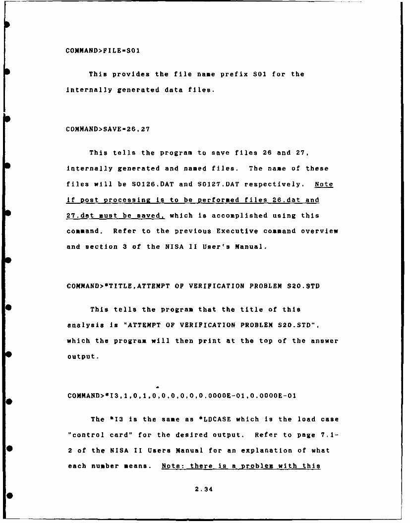
COMMAND>FILE=SO1

This provides the file name prefix SOl for the

internally generated data files.

COMMAND>SAVE=26,27

This tells the program to save files 26 and 27,

internally generated and named files. The name of these

files will be S0126.DAT and S0127.DAT respectively. Note

if post processing is to be performed files 26.dat and

27.dat must be saved, which is accomplished using this

command. Refer to the previous Executive command overview

and section 3 of the NISA II User's Manual.

COMMAND>OTITLE,ATTEMPT OF VERIFICATION PROBLEM S20.STD

* This tells the program that the title of this

analysis is "ATTEMPT OF VERIFICATION PROBLEM S20.STD",

which the program will then print at the top of the answer

output.

*

COMMAND>*I3,1,0,1,0,.0,0,0,0.0OOE-01,0.OOOOE-O1

The *13 is the same as *LDCASE which is the load case

"control card" for the desired output. Refer to page 7.1-

* 2 of the NISA II Users Manual for an explanation of what

each number means. Note: there is a problem with this

2.34

command on the PC version of 88.7. No matter what entry

is placed after "*13," the program automatically changes

it to "0.1.3.0.0.4,0" on the *LDCASE card in the "(file

name).NIS" file. The "(file name).NIS file is the file

that the NISA II program actually uses for the analysis.

Therefore, if different output than what is specified with

"0,1,3,0,0,4,0" is desired, the *LDCASE line in the (file

name).NIS file must be manually changed. This can be

accomplished using a text or line editor like EDLIN.

COMMAND>*14.I,POINT LOAD AT BEAM'S CENTER

The *14 is the same as *LCTITLE which means load case

title. This is the title for the specific load case. In

this example the title "POINT LOAD AT BEAM'S CENTER" is

assigned to load case 1. If there were multiple load

cases, as discussed In "FORCE,ADD,..." above, multiple

load case title cards can be used, one for each load case.

In the description for entry 5 of "FORCEADD..." two

loadings were discussed, one force and one moment. In

that case the input could be:

COMMAND>*f4,1,POINT LOAD

COMMAND>*I4,2,MOMENT

or what ever the desired titles were. The program will

then place the specified title at the heading of the

answers for each load case.

2.35

COMKAND>QUI

Quits the insert mode.

COMMAND>QUI

Quits the DEC mode.

COMMAND>WRI,NIA,SO1.NIS

This takes the above data just input during this

session and writes a "NISA" file called "SOl.NIS" that the

program uses for it's analysis.

COKMAND>WRI,DBSSO1.BIN

This takes the above data and writes a binary data

base file called "SOl.BIN".

COMMAND>END

This ends the session.

Data Base File: At this time the program will ask If a

data base file DISP.BIN is to be written. Since this has

already been done with the WRI.DBS,SO1.BIN command above,

answer no "N".

2.36

The model is now ready to be analyzed. Refer to the

previous section "Program Usage" for guidance on how to

perform the analysis.

2.37

COMMAND INPUT DEMONSTRATION

In an attempt to assist the unfamiliar user with

understanding what the various DISPLAY-PRE commands

actually do, the demonstration below provides a pictorial

description of some of the various commands required in

the previous verification problem. This demonstration

does not contain all required commands only a few to

provide an Idea of how the commands work.

GRD.ADD.1,0/O/O This creates a point at coordinates

(0,0.0).

0I

ORD.TRS.1,2,15 This creates grid #2 by translating

grid #1 15 units in the X direction.

0. 0' 2

2.38

LIN.2GD.I.2.l This creates line #1 between grids *1

and #2.

FEGBAR.1 ...8/13,1/1 This cr-eates 8 elements of NKTP

type *13 along line #1, and assigns MID-i and PID-1. Note

there is a node created at the end of each element.

LINTRS,1,2./-1O This creates line *2 by translating

line *1 -10 units in the Y direction.

2.39

FEG.BAR,2,..8/13 This creates 8 elements of NKTP type

13 along line *2 and allows the program to automatically

number them. Again, as mentlond above, each element has a

node at each end.

•( a-.,) (u%-oJ

ELE.DEL,9T16 This deletes elements 9 through 16.

However, nodes 10 to 18 remain.

0 @0® @0 0 @ 00®

ELE,ADD,9,18/1//2,1/lO This adds element 9, of NKTP

type 18 and PID #2, between nodes 1 and 10.

2.40

ELE.ADD.17.42/1//5.9/18 This adds element 17, of NKTP

type 42 and PID *5 between nodes 9 and 18. Note the steps

to add elements 10 to 16 were not shown. but would

consists of basically the same command.

I I Z 3 v ,1 *

, 2.41

VERIFICATION PROBLEM 5.5 (

* TITLE:Natural frequencies of a simply supported square plate

ELEMENT TYPE:* 3-D general shell element (NKTP - 20, NORDR a 2)

PROBLEM:

The first five natural frequencies of a simply supported square plate, with dimensions as shown inFig. 5.5.1, are to be computed.

0PROPERTIES:

Material:EX - l0.5E6 psi (Modulus of elasticity)NUXY = 0.3333 (PoLiss's ratio)

* DENS a 2.588E-4 b 2i4 (Mass density)

Geomeby:t - l.Oin (t m) ("FINITE ELEMENT MODEL:

The plate is modeled using sixteen j-D general shell elements (W =20, NORDR = 2). The nodes onthe perhery of the plifi are a up- n In the nomal (LM) dreaon. l-plue aw ladou (X ad UY)for all the nodes art conuhubd to obtan only the beai t modes.

* SOLUTION PROCEDURE:Conventonl subspme iteration and lumped mass mamix foumulation ate used to extract the dgeavalues.

RESULTS & COMPARISON:The fim five natural frequencies of the simply supported plate obtained from NISA anm compared to the

* theoretical (Ref. [1]) values in Table 5.5.1. The mode shape plots are shown in Fig. 5.5.2 through 5.5.6.

REFERENCE:

1. S. ibmoshenko, D. H. Young, and W. Weaver, Jr., "Vibration Problem in Engineering". 4th edition,John Wiley & Saos, New York (1974).

04

• 2.42

trAgMVaweC AflhLyMs tJl A venticauo Manual

13 75 77 79 81

551 __ 5 59 61P5- - 1,63

() 48"37 39 141 43 4

-9 -2- 23-50

(I Figure PaIt 'W Ekmaiz blob for a Skupa Saped Sqame'Fla

Figure 5.5.2 Mode No. 1: Frequency -83.979 Hz

2.43

GR), TRS, I , 2, 48LIN,2GD, 1,2,1LIN,TRS,1,2,t 0/48PfAT,2LN, 1,2,1FEG,QUA,l .. ,2/4/4/20

DISFP-,ADD, 1/9/57/65,1 ()/C)/C)/C/ODISP,ADD,2T6/58T64, 1,Ci/0/C'//CiDISP,ADD, IC/14Tl5/2M: 124/2eT29/'37-T3B,/42T43/51r52-./56,1,///DISP,ADD, 11T113/16T*225TC-7/0T3I-:6/.79TA1/44T50/53T.-55, 1.,0/0DECINS(ANAL=E I ENF ILE = EuSAVE=26..27F:ESE=ON

EIGE=SUBES,CONVMASS=L UMPED*LDCASE, 1*E IGCNTL, 5, 0,20, 0, 0. 0, 0. 0,1. OE-*MDDEO, 1,1,1,1*EIGO, 1,1,0,3,1 ,c, 1

QU I

WRI ,NISA,ECI . NISWRI ,DBS,E01 .BINENDN

2.44

E: X 1-,UI I VE

ANAL- I GE-NF LE- 4-(, ISAVE 26,27R:SE ONAUTO ONEI GE=SUBS,CONVMASS=LUMPED*ELTYPE

1, 20, 2*RCTABLE

1, 01 . 00)C00), 1.ocou. .)~:U 009 . 0¢100,) . " -'(: 1 *-:A:;. .:)?' .""

*ELEMEN-", 1, i, 1, 0

6, 2, 3. ii 7 ,'2' 16. ,

1" 17 I,- 1 17, 25Z6, 1. 91, 0

17.., 1i, 19, 26, 27125

*3, 6 7, 13"$ 21. 20. 1'T. 12'-4, 1, 1, 1, 0

19, 20, 21, 27, .5-, 34, 33, 26:,

B,, , , 015, 16, 17, 25, 31, 30, 35, 24,

6, 1, 1, 1, 017, 18, 19, 26, 33, 32, 31, 25,7, 1, 1, 1, 0

19, 20, 21, 27, 35, 34, 33, 26,8, 1, 1, 1, 0

21, 22, 23, 28, 37, 361 35, 27,91, 1, 1, 1, 0

29, 30, 31, 39, 451, 44, 43, 38,10, 1, 1, 1, 031, 32, 33, 40, 47, 46, 45, 39,11, 1, 1, 1, 045, 4, 35, 41, 49, 48, 47, 40,12, 1, 1, 1, 035, 36, 37, 42, 51, 50, 49, 41 ,13, 1, 1, 1, 043, 44, 45, 53, 59, 58, 57, 52,14, 1, 1, 1, 045, 46, 47, 54, 61, 80, 59, 53,15, 1, 1, 1, 04 4, 63, 62, 61, 54,

16, 1, 1, 1, 049, 50, 51 , 56, 65, 64, 63, "NODE S

1 , ,O . 0000) 0.*0000 , 0. 0000 ,

2 , 6. 0000, 1.0000, 0.0000,3 ,,,, 12.0000, 0.0000, 0.0000,4 , ,,, 18. 0000, 0.0000, O. 0000,5 , , 24. 0000, 0.0000, 0. 0000,6 , ,, 30. 0000, 0.0000, 0.0000,7 , ,,, 36. 0000, O.0000, 0. 0000,8 ,,, 42. 0000, O. 0000, O. 0000,9 ,,,, 48.0000, 0.0000, 0.0000,

2.45

. , 9 I I) 111 I I I I II~ I, I I ii i

l '.' s ,t (. (,-r r] p , ()QUO() I ) ( 00

10 , , , , 2. 0 (, 6. 0000, o. - ,12 "24 .000 , O(QOOj C)

1 , ,,6. " J000 6... 00o 0 .

14 , ,) () ,) 48. ( 00 0 6. OCIC, 0O. 00 ,1s , ,, O. O1lO0, 12. c0(10 , 0. ( o00 ,16 , ,,, 6. 0000, 12. 0000, 0. 0000 ,1'7 ,,2, , 1. 0r0,O 12. 000, 0. 000 C),16 , , , , . 0(-000, 12. O000, (. oo0019 ,,,, 24. 0000, 12. 0000, C. 0:000,320 ,,,, 3(1.000, 12. 0000, . OO,

21. .. 3 * " ( "0: 12. Oooo *, 0. .'c'o,22 42. 0000, 12. 0000, C.0000-- , , , *'6*0(0 . 2.o ) ,. C()0(),24 C) UO((). *. 20~ . 0(00,2 . . 2, O *.0011- , 1,. ()(000, C).0(]0

25 ,, *, 12.0000, 1 .000 0 .0000,

24. " ..... c8.000026 , ,, . 6. (303(, 24 (0 .0000,)C

17 ,4. 0000, :1: 24. 0000, t. 000001.0 0.00033"24. 24. 0000, 0000,

.4 , ., . , 0 00 4* 00, 0.00

SQ 24.0000, 0.0000,36 ,,,, 46. 0000" .00, 0.

37 ,1., 8 12.000 24.0000, 0.0000,SB ,,, 0.0000, 24. 0000, 0 .0000,39 ,,, , 2 4. , 00000, 0. 0000,34 ,,,, 24.0000, 24.0000, 0.0000,45 ,,, 36.0000, 24.0000, 0.0000,36 ,,, 42.0000, 24.0000, 0.0000,37 ,,,, 48.0000, 24.0000, 0.00001•38 ,,,, 0.0000, 30.0000, 0.0000,4 ,,,, 12.0000, 30.0000, 0.0000,40 , , , , 24.0000, 30.0000, 0.0000,41 ,,,, Z6.0000, 3.0000, 0.0000,42 ,i, 48.0000, 30.0000, 0.0000,43 ,,,, 0O.0000, 36.0000, 0.0000,44 gig, 6. 0000, 36.0000, 0.0000,45 ,,,, 12.0000, 36.0000, 0.0000,46 ,, ,, 18. 0000, 36.0000, 0.0000,47 ,I , 24.0000, 36.0000, 0.0000,4 , , , , 3:0000, 42.0000, 0.0000,

, ,,, 36.0000, 42.0000, 0.0000,50 ,,,, 48.0000t 36.0000, 0.0000,

* 57 ,,, 4. 0000, 836.0000, 0. 0000,

52 ,, , , 6. 0000, 42. 0000, 0. 0000,53 , , , , 12.00001 42.0000, 0.0000,54 1,,, 24.0000, 42.0000, 0.0000,55 , , , , 24.0000, 42. 0000, 0.0000,56 , , , , 48. 0000, 42. 0000, 0. 0000,57 9,,, 0.00001 4B.O000, 0.0000,

5B , , ,, 6. 00009 48.000, O .000,59 9, ,, 12. 00C), 48.0000, 0 O CO0,60 9,,, 1S. 0000 , 48. 000C0, O.C)0C0O61 ,,,1, 24. 0000, 48. 0000' 0. 0000,62 ,,,, 3"1.00 48. 0000, '. 0000,

•63 ,,, j 9 6.Q0 00C, 4B.0000, 0.0000,

64 ,,,, 42.0000, 48.0000, 0.0000,65 , , , , 48.0000, 48.0000, 0.0000,

2.46

*12t,0 , 20 0), 0. 0 0. 0 ,1 . 0L-5

*SPDISP**SET ID I

I , ROTY , 0.0001 ,ROTX, 0.(:000000CI uz , o. clI(:)oCl:I1 ,UY 0 00C000")I ,ux 0. (10000C)2, ROrY, 0:. CI0CCC:CIC2, UZ C) .cc(:Cc

t li Y

4 , uZ 0. 0I00)(0

5 , uv Y, 0. 000000,lIX 0. 000000

5, OY, 0. 0000005,uX , 0J.C000006,UOY , 0.0000006,UX 0.0000000,ROY, 0.0000006,UZ , 0.0000007,UDY , 0.0000007,LJX 0.0000007,UDY, 0.0000007,UZ 0.0000007,UDY , 0. 0000007,UX 0.0000008 ,DY, 0.000000B,UZ 0.0000008,UOY , 0. 0000(18,UCX , 0.0000009, RTY 0. 0000009 ,ROT 0.0000009,UZ 0.00000010,UY , 0.000000I9,uX 0.000000Cl~10,ROTX 0.00000010 ,U , 0. 0000010,UY , 0.000000i0,UX, 0.000000

$.guy 0.00000012,UY 0.000000123,UX 0.00000013,UY 0.000000

14,RCTX, 0. 00000014,UZ , 0.00000014,UY , 0.00000014,UX , 0.000000

2.47

1 , po-rx , 0. .))(:15 , i" I ,- . () f) 1.) (.1 ()(-

16, UY , ). 00C1,00

17 , UX , C))UU

18 *U Y c o o* ~~~~19, LXC.(xYi:c

19 ,ULX 0 0 0 (1icC)

20 UX C (). CICIC)c

-2 1 , UY Cl* u~lcl:Icl* 21 UX 0. 00000iO

22,U , *y (:)Oo:)c)(ci

2Z ,ROT X, 0. 000C0oiO2Z;, uz C) 00000CcM)(:23 ,UY , 0. 000000

* 23,UX , 0. 00000024,ROTX, 0.00000024,UZ , C.000OC)24,UY 0 .000000o24,UX , 0.00000025,UY 0.000000

* 25,UX , 0.00000026,UY 0 0.00OO026,UX , 0.00000027,UY 0.00000027,UX , 0.00000028,RDTX, 0.0(00000

*28, UZ , 0. 000000(28,UV 0.000000~i28,LJX Cl.ocoo29,ROTX, 0.00000029,UZ , 0.00000c)29,UY 0 c.OO000O

* 29, UX ()i. 00000C'Z30,UY , 0.00000030,UX , C.Ooo7,1 ,UY , 0.000000O1 UX 0. 000000

-32,UY C).000000*32, UX , ) .000000

33 ,UY , Cu). 000000o3 3,U ,x 0. 00000034,UY , 0.OOOOC'0341~UX , 0000000(

2.48

O~JtU q , 1 C). 00000036, UY 0. 000000C2)C

:;6, UX . OOCIO0007 ,F -~o-rx , ) 'OQc 0c)

.:% ,uz ,(-) -0c0c)

Z7, UY 0. U00000037 , UX , 0. 0000:00

"g R rx , ) C))CCc)uz , ().cloooo10

U Y *. ).))).3ux 0000C00)O)C

79U .9w 0.0)C00039I~ , UX U 0 (0000040,UY , C.OO0)040), ux C)o. 0c00041,UY Q'. OO)C)()C(:c41 ,UY 0. 000)OC0042,ROTX, 0.00000042,UZ , 0.00000042,UY , 0.00000042,UX 1 0.00000043,ROTX, 0.00000043,UZ , 0.00000043,UY , 0.00000043,UX , 0.00000044,UY , 0.000000447 UX 0.00000045,UY 0.00000045,UX , 0.00000046,UY , 0.00000046,UX , 0.00000047,UY , 0.00000047,UX , 0.000000

48,UY0.00000048,UX , 0.00000049,UY , 0.00000049,UX , 0.0000005, UY 0C. 000000

so,Lx , 0.00000051 ,ROTX, 0.00000051,UZ , 0.00000051,UY , 40.00000051,UX , 0. 00000052,ROTX, 0.00000052,UZ , 0. 000000C)52,UY , 0.00000052,UX , 0.00000053qUY 0.00000053,UX , 0.00000054,UY , l ('00000054,UX 9 0.000000

2.49

,. u x , 0. (10(1(2 Ot56, ROT X, o 0(200c~l56,UZ , .(000000256,* UY 1) ':0 (1)

5*7,ROTY', 000001".)0(:(c57 ,ROTX , 0.00000))C(:57 UJ Z I CCC(':

597, UY 0 ). 0000

"-;SUY 0. 00000058,U LA 0. (00000

51 , ROTY, 000000091,UZ 0 0.00000C6, UY , 000000061,UX 0 :.0000060,ROTY, 0. 00000060,UZ , 0.00000062,UY , 0.00000060,UX "'I.00000063, ROTY, 0.00000061,UZ , 0.00000061,UY 000061,UX , 0.00000064 ,ROTY, 0. 00000064,UZ 0. 00000064,UY 0.000000629UX , 0.000100065, ROTh', 0. 000000

64,ROTY, 0. olovOOOo64,UZ , 0.00000064,UY 0 .000000

65 ,RLIX, 0.*0000002

*MOD1EO1,1,1,1*E 11O1 , ),3, 1 , I

*ENDDATA

2.50


COMMAND>GRDADD, ,0/0/0

This adds a grid (a point in 3-D space), calls it

grid #1, and puts it at coordinates (0,0,0).


This makes grid *2 by "translating" grid *1 48 units

in the X direction. Actually it translates grid #1 48/0/0

units where the format Is X/Y/Z: since there are no "O"s

typed in. they are automatically assigned. If It was

desired that *2 be placed 48 units in the Y direction, the

Input would be either "GRD,TRS,1,2,0/48" or

"GRD,TRS,1,2,/48". Default values are "0".

COMMAND>LIN,2GD,1.2.1

This creates a line starting at grid *1 and ending at

grid *2, calling it line *1. The format is

"LIN,2GD,starting grid *,ending grid C".a

COMMAND>LIN,TRS,1,2,0/48

This creates line *2 by translating line *1 48 units

in the Y direction. This command could be either be input

as is or as "LIN,TRS,1,2,/48". The format is

2.51

0

"LIN,TRS,3,4,5A/5B/5C" where:

Entry 3 in the line to be translated.

Entry 4 is the line * to be created.

Entry 5 is the direction (X/Y/Z) entry 3 is to

be translated in. Default values in this entry

are "O"s.

COMMAND>PAT,2LN,l,2,1

PAT stands for patch, which is defined as a plate of

defined size in 2 D space or a surface of defined size in

3 D space.. This entry creates patch #1 between lines *1

and #2 with the following format: "PAT,2LN.LINE ID #1.

LINE ID *2, PATCH #". Refer to the example at the end of

verification problem break down for an example of how a

is created and what it looks like.

COMMAND>FEG,QUA,I, ,.2/4/4/20


entry creates a group of 16 quadrilateral shell elements,A

4 elements by 4 elements, in the plate created by the

above patch. This is accomplished with the following

format: "FEGQUA,3,4,5.6A/6B/6C/6D.7A/7B/7C/7D where:

Entry 3 is the patch ID number that is to be

"FEGED".

Entry 4 is element ID list. This is the list of

0 2.52

the element numbers to be created. If left

blank the program will automatically number the

elements being created.

Entry 5 is the list of node numbers to be

created. Like the element entry above if this

entry is left blank the program will

automatically number the nodes.

Entry 6A is the order of the elements to be

created. In this case the elements are second

order shell elements, of NKTP type 20, and

contain 8 nodes per element. Refer to the

Element Section of the DISPLAY II User's Manual.

Entry 6B and 6C are the number of elements to be

generated along the parametric directions Cl and

C2. Parametric directions are internally

assigned by the program to two edges of a patch

and three edges of a hyperpatch and are used by

the program for defining mesh density of the

patch. For example suppose it is desired to

"break" a line 1/3 of the way from the end.

Where is the end and where is the start? The4

program uses parametric directions to show where

the start (where the directions intersect) and

end Is. Refer to pages 2.2-7 to 2.2-10 of the


Entry 6D is the NKTP *, which stands for the

elements type Identification number. Each

0 2.53

element type has a different NKTP F. For an

explanation of exactly what a specific NKTP #


NISA II User's Manual, pages 4.0-1 to 4.120-5.

Entry 7A and 7B are the material and property ID

Vs respectfully. This set of #s. assigned to

one or more elements, is used later in the input

phase for assigning actual properties. If left

blank the program automatically assigns a

material ID * of 1 and a property ID * of 1. In

this case all the elements have the same

material characteristics and property

characteristics and therefore all have the same

MID # and the same PID #.

Entry 7C and 7D are the zoom values to be

assigned along the parametric directions

discussed in entry 6B and 6C above. If left

blank the program assigns zoom - 1 to both.

COMMAND>PROP,ADD,1,1/1/1/1/1/1/1/1

This adds a thickness of 1 unit to all eight

nodes of the elements with PID = 1 with the following

format "PROP.ADD,3,4A/4B/4C..." where:

Entry 3 is the property index * (PID).


defined by tie element type with each different

2.54

property separated by a /. Refer to the

specific element type In the element library

section of the NISA II User's Manual for more

info on what properties are listed here.

COMMAND>MAT,ADD,l,1O.5E6/O.3333////////2.5879E-4

This adds the material properties of modulus of

elasticity (EX) = 10.5E6 psi, Poisson's ratio (NUXY) =

0.333 and mass density = 2.5879E-4 lbs.-sec squared per

inches to the fourth power to all the elements with

material ID #1. This is accomplished with the following

format: MAT,ADD.3,4A/4B/4C..." where:

Entry 3 is the material ID I.




type with each separate property being separated

by a slash "".

COMMAND>DISP,ADD, 1/9/57/65,1.0/0/0/0/0

This constrains nodes 1,9,57, and 65 in the X, Y, Z,

Rotation In X and Rotation in Y. and assigns a constraint

ID * of I with the following f %at:

"DISP,ADD,3A/3B/3C .... 4,5A-5F". where:

Entry 3 is the list of nodes to be constrained.

2.55


* under which the constraints are specified.


are constrained. This is accomplished by

* placing a "0" in the degree of freedom that must


"X/Y/Z/ROTX/ROTY/ROTZ". Consecutive slashes or

* constrained directions not listed, indicate a

null entry which the program either ignores or

places a default value in that place. In this

* case the program ignores the null entries. For

more information on null entries refer to the

general command rules previously addressed in

* this chapter of to pages 2.1-3 to 2.1-6 of the


COMMAND>DEC


* Executive Commands. For more info on executive commands

refer to the previous Executive command overview and page

7.10-1 of the DISPLAY !I User's Manual.

COMMAND>INS

* This places the program in the mode to allow the

insertion of data lines.

2.56

COMMAND>ANAL=EIGEN


performed is an EIGENVALUE analysis.

COMMAND>FILE=EOI

This provides the file name prefix EO for the

internally generated binary data files.

COMMAND>SAVE=26,27

This tells the program to save the internally

generated binary data files 26 and 27. The names of these

files will be EO126.dat and E0127.dat respectively. Note

this command must be used to save the data files 26 and

27. which are required for post-processing or dynamic

analysis.

COMMAND>RESE=ON

This command tells the program to look at the

numbering of the elements and resequence them (ie renumber

them internally) to make the finite element analysis more

efficient. The input of this command is not required as

the program will automatically perform this function.

When creating a finite element model there is definite

"pecking order" of how elements and nodes should be

2.57

numbered. The analysis of a model that does not follow

this order will take longer than one that does. This

command has the program check the model to see If it

conforms to the "pecking order". If the model does not

then the program will internally change the element

numbering so that it does. The change will not effect the

user as it is transparent to the user and the element IDs

that the user uses are not changed. For more info refer

page 5.3-5 of the NISA II User's Manual

COMMAND>AUTO-ON

This command activates the automatic spurious normal

rotation constraint for shells. This Input is not

specifically required as the default mode Is for this to

be on. Nodes In basic shell theory have 5 degrees of

freedom. When transferring a model from the non-global

system to a global system rotation in the theta Z

direction may occur. Additionally rotation perpendicular

to the theta Z direction may occur. If this happens then

the shell (ie model) will not be defined and therefore

cannot be solved. -Having the AUTO CONSTRAINT on will

constrain this perpendicular rotation, thereby allowing

the model to be defined.

2.58

0

COMMAND>EIGE-SUBS,CONV

This command tells the program that the elgenvalue

extraction method is to be conventional subspace. This

command produces some effect on the speed of the analysis.

If the eigenvalues are far apart then having the method be

accelerated subspace will cause the program to

aggressively shift the frequencies in order to speed up

the convergence onto the natural frequencies. Refer to

pages 3.5-1 to 3.5-4 and 5.3-6 in the NISA II User's

Manual.

COMMAND>MASS-LUMPED

This command tells the program to activate the lumped

matrix formulation, ie it tells the program to solve the

stiffness matrix diagonally instead of consistent with the

way the matrix was developed. Refer to page 3.5-5 of the

NISA II User's Manual.

COMMAND>*LDCASE,1

This is the load case "control card" for the desired

output. Refer to page 7.1-2 of the NISA II User's Manual

for an explanation of what the number(s) following the

card heading mean. Note when performing an Eigenvalue

analysis this card Is not applicable. However. using this

card was the only method the author found of "saving" the

2.59

displacement constraints that were input previously. A

more difficult method of inputing the displacement

constraints would be to input them directly into the NIS

file using a text or line editor, like EDLIJN. Therefore

the user should either use this command to save the

displacement constraints and then delete the two specific

load case lines in the NIS file by using a text or line

editor, like EDLIN, or input the displacement constraints

directly into the NIS file. (The NIS file will be

explained below.) The load case lines that need to be

deleted consists of one line containing *LDCASE and a

second line containing the string of numbers input

immediately after the word *LDCASE above.

CONNAND>*EIGCNTL,5,0,20,0,0.0,0.O,1.OE-5

This command tells the program what the control

parameters are for the elgenvalue extraction. Refer to

pages 7.1-5 to 7.1-6a of the NISA II User's Manual for an

explanation of what each number means.

COMMAND>*ODEO,1.1,1,1

This command tells the program what modes the

analysis is required on. The format is "MODEO,2,3,4,5"

where:

Entry 2 is the first mode number to be

2.60

analyzed.

Entry 3 is the last mode number to be analyzed.

Entry 4 is the Increment between the first and

last modes that are to be analyzed.

Entry 5 is the output ID # that refers to the ID

# listed in the output command *EIGO.

For more info refer to page 7.1-15 of the NISA II User's

Manual.

COMMAND>*EIGO.1,1,0,3,1,0,1

This command tells the program what output options

to provide. For an explanation of what each number means

refer to pages 7.5-2 to 7.5-4 of the NISA II User's

Manual.

Note: there seems to be a problem with the MODEO and EIGO

commands beinz accepted by the DISPLAY-PRE program and

then saved in the NIS. file. As a result the above

commands must be inputed directly into the ".NIS" file

using either a text or line editor. This is accomplished

with the following format:

line x: *MODEO

line x+1: modeo data

line x+2: *EIGO

line x+3: eigo data

where line x+4 is the ENDDATA line

2.61

The EIGO line must be the first output line listed. If

any other output is requested (Example REGIONS, the

regions for averaged nodal stresses printout; STRSFIL, the

nodal stress filtering data; etc.; it must be listed after

the EIGO data line. Refer to Section 7.5 OUTPUT CONTROL

DATA of the NISA II User's Manual.

COMMAND>QUI


COMMAND>QUI

Quits the DEC mode.

COMMAND>WRI,NISAEOI.NIS

This takes the above data Just Input during this

session and writes a "NISA" file called "EO1.NIS" that the

program uses for it's analysis.

COMMAND>WRI,DBS,EOI.BIN

This takes the above data and writes a binary data

base file called "EOI.BIN"

2.62

CONKAND>END


Data Base File: At this time the program will ask if a


already been done with the WRI,DBS,EOI.BIN command above,

answer no "N".

The model is now ready to be analyzed. Refer to the

previous section "Program Usage" for guidance on how to

perform the analysis.

2

0

2.83

COMMAND INPUT DEMONSTRATION

In an attempt to assist the unfamiliar user with

understanding what the various DISPLAY-PRE commands

actually do. specifically the creation of a patch, the

demonstration below provides a pictorial description of

some of the various commands required in the previous

verification problem. This demonstration does not contain

all required commands only a few to provide an idea of how

the commands work.

GRDADD,1.0/0/0 This creates a point at coordinat.

(0,0,0).

I

GRD,TRS.1,2,48 This creates point (grid) *2 by

translating grid #1 48 units in the X direction.

2.6

~2.64

LIN.GD.I.2. This creates line *1 between grids #1

and *2.

I

LIN.TRS. 2,0/48 This creates line *2 by

translating line #1 48 units in the Y direction.

2.65

PAT,2LN.1.2.1 This creates patch #1 between lines *1

and *2.

I

PEG,QUA~l.,.2/4/4/20 This creates a group of 16

quadrillateral shell elements of NORDR 2, 4 elements by 4

elements. in the patch created above. Due to space

limitation not all the nodes are numbered.

S7 T so 6# 64

,, 91DY4 1 4& 42 LV ,

Ez1V 31

7.

2.66

I ranUau UlynamIc Analyss NISA Verification Manual

VERIFICATION PROBLEM 6.3 -

TITLE:

Transient response of a beam subjected to distributed load

ELEMENT TYPE:2-D beam element 0(XrP - 13, NORDR - 1)2-D translational spring element (NKTP = 18)

PROBLEM:A beam supported by two springs of stiffness K/2 = n4EI/2L3 at its ends, as shown in Fig. 6.3.1, issubjected to a distributed load given by:

p(x) = 1-2 IxL for -L2 < x S L/2

The variation of the load with time is shown in Fig. 6.3.2. Lateral motion of the beam is constrained. Thenatural frequencies and time history response of the mid-point of the beam are to be computed.

PROPERTIES:

EX W 3.Ox 107 pid 0Mostu aotfmdcky)NUXY = 03 - qdasan'a o)DENS = 0.00072 lbs-sec2 as density)CrostsectloxA = 4.0 (Cru.4ecdml ma)ZZ - 1.3333 in4 (Moment of Iunla about beam Z-ais)

FINITE ELEMENT MODEL:The fim element model is shown in Fig. 6.3.3. Since the aled load and d3, systm are symmetrc, onlyone half of the beam is modeled. Symmetry boundary condos (UX - 0.0. ROTZ = 0.0) e applied atnode 1. Lateralmotionis costrined(UX=0.0 at nodes 2 md 3. and node4is flxed(UX=0.0,UY = 0.0).

SOLUTION PROCEDURE:Consistent mass matrix fbmulaticn and subspace iteration technique is used in evaluating the naturalfrequencies. Fust two symmetric modes are used for the transient dynamic analysis.

RESULTS & COMPARISON:The natural frequencs of the first two symmetric modes are compared to the theoretical values inTable 6.3.1. The peak transient response of the mid-point of tb- beam is compared to the theoretical valuein Table 6.3.2. The displacement history of the mid-point of the beam is shown in Fig. 6.3.4.

2.67

x

ligure 6.3.1 Beam with Distributed Load

P(t)

0.0 0.02 0.04

TDg

ligVr-s 6.3.2 loed-V~I RAM

ligure 6.3.3 Miite 7!lumt Model

2.68

GRD,ADD, 1 ,0/01/0:GRD,TRS, 1,2,40LIN,2GD, 1,2d,1FEG,BAR, 1,,,2/l3, 1/1NOD ,ADD ,4,40)/-4ELE,ADD,3., 18/1//2,-"/4DISP,ADD, 1,1,0/////ODISPIADD,2T3,1I,O)DISP,ADD,4,1I,0/0PROP, ADD, 1, 4. 1i. 333MAT,ADD, ,:.cE7/0.:.////72E-PROP, ADD, 2 Bc) 85E3DECINSANAL=E IGENVALUEAUTOCONSTR I NT=OFFRE SEQUENCING OF ELEMENT6=ONFILE=ETD01SAVE=26 ,27EIGEN EXTRACTION=SUBSPACEMASS MATRIX FORMULATION=CONSISTENT*TITLE,ATTEMPT OF VERIFICATION PROBLEM ET03. STD,*12,59-1 ,2090,0.0,0.0,1.OE-5

WRI ,NISA,ETDO1 .NISWRI ,DBS,ETDO1.BINENDN

2.69

** EXECU" IV'ANAL=E I GENVALUL

* AUTOCONSTRAINT=OFFRESEQUENCING OF ELEMENTS=O!:F ILE=ETDO1SAVE=26,27EIBEN EXTRACTION=SUBSPACEMASS MATRIX FORMULATION=CONSISTENT

**TITLEATTEMPT OF VERIFICATION FROB-FLEM ETO5.STD*ELTYPE

1, 1s, :12, Is, I

* 1, 24 . J ... .....

2. 1380 5.00 00,

*ELEMENT1, 1, 1, 1, C?

* 172, 1 1, 1 , 0

, 0, 2, 2, 03, 4

*NODES• 1 s,,,, 0000, 1.0 0 .'}0

2 , , , , 20 . 0000, . (00(:)0 0.000 ,

3 ,,,, 40.000 , 0.0000, 0.0000,4 ,,,, 40.0000, -4.0000, 0.0000,

*MATERIALEX , 1 , , 0.30000E+08

* NUXY , 1 , ,0.3C000E+00DENS 1 , , 0. 72800E-03

*125-i , 20 ,0o,0o.0o,0. o, I. CE-5

*SPD I SF** SET ID 1

* 1 , ROI Z, 0.00001 , U X , 0. 00:0002,UX , 0. 0000007,Ux , 0. 0000004, UY 0 C.0 0000C,_U4 ,LIX 0 U. 000000

S2*ENDATA

• 2.70


COMMAND>GRDADD,I,0/0/0




This makes grid *2 by "translating" grid *1 40 units

in the X direction. Actu .ly it translates grid *1 40/0/0

units where the format is X/Y/Z: since there are no "O"s

typed in, they are automaticaliy assigned. If it was

desired that *2 be placed 40 units In the Y direction, the

input would be either "GRD,TRS,1.2,0/40" or

"GRD,TRS,1,2,/40". Default values are "0".

COMMAND> LIN,2GD,1,2,1

This creates a line starting at grid *1 and ending at

grid *2, calling it line #1. The format is

"LIN,2GD,starting grid *,ending grid ".

COMMAND>FEG,BAR,l, ,, 2/13,1/1

FEG %ands for "Finite Element Generation". This


ype 13), in the global coordinate system, assigning a

2.71

material ID # of 1 and a property ID * of 1, and a zoom of




"FEGBAR.3,4,5.6A/6B/6C,7A/7B/7C" where:

Entry 3 is the number of lines to be "FEGED".


left blank the program will automatically number

the elements.

Entry 5 is the list of generated nodes. If left


nodes.




element type Identification number. Each

element type has a different NKTP *. For an




Entry 6C is the node * that has a local


This entry is used only If the beam is not to be

defined in the global coordinate system (ie the

Cartesian. Cylindrical, or Spherical systems).

At times it :s more convenient to refer to items

with a local coordinate system, for example a

2.72

force or displacement constraint may be defined

with directions which are not aligned with the

global coordinate system. For more information

on local coordinate systems refer to pages 3.2-1

to 3.2-4 of the NISA II User's Manual.


Vs respectfully. This set of #s, assigned to

one or more elements, is used later in the input



material ID * of I and a property ID * of 1.




etc.) with some of the elements having one

geometric property and others having a different

geometric property. As a result this group of

elements would have one material ID * and two

property ID #s.

Entry 7C is the zoom factor, le the length of

the last element to length of the first element.

If all elements are the same length then the

zoom - 1. If left blank the program


information and a pictorial representation refer

to page B-3 of the DISPLAY II User's Manual.

2.73

COMMAND>NOD,ADD,4,40/-4

This command adds a node at coordinates (40,-4,0) and

calls it node * 4. This is accomplished with the

following format: "NOD,ADD,3,4A/4B/4C/4D" where:

Entry 3 is the node * to be generated.

Entry 4A. 4B, & 4C are the (X/Y/Z) coordinates

of the node.

Entry 4C is the local coordinate system in which

the coordinates are to be specified. If this is

left blank then the node is in the global

system.

COMMAND>ELE,ADD,3,18/1//2,3/4

This adds an element *3 with NKTP = 18, order - 1,

property ID * - 2 between nodes 3 and 4, using the

following format: "ELE,ADD,3,4A/4B/4C/4D,5A/5B,6" where:

Entry 3 is the element * to be added. If this

is left blank the program will automatically

assign a number.


FEG description above).

Entry 4B is the order #. Some elements only

have one order, NORDR-I, others have many

depending on the element type. For a pictorial


to section 4, the "element library" of the NISA

2.74

II User's Manual; specifically NKTP #s

1,2,3,4,5,& 32 provide good examples of some of


Entry 4C Is the material ID *. This # Is used

later in the input phase to assign actual

material properties to this element.

Entry 4D Is the property ID #. (See entry 7B


Entry SA & 5B are the two nodes that define the

element. Most elements require two nodes, one

at each end. However since this particular

element is a mass concentration it only requires

one node.


defined vector used In establishing a local


elements of NKTP - 11, 12, & 38.

COMMAND>DISPADD,I,1.0/////O

This constrains node #1 in the X and ROTZ directions

and assigns a constraint ID * of 1 with the following

format: "DISP.ADD,3A/3B/3C...,4.5A-5F", where:




Entry 5A to 5F nre the degree(s) of freedom that

2.75




"X/Y/i/ROTX/ROTY/ROTZ". Consecutive slashes or

constrained directions not listed, indicate a



case the program ignores the null entries. For



this chapter of to pages 2.1-3 to 2.1-6 of the


COMMAND>PROPADD.1,4./1.3333

This adds a cross sectional area of 4.0 inches

squared and a moment of inertia on 1.3333 inches to the

forth to all the elements with property ID * 1. This is

accomplished with the following format

"PROP,ADD,3,4A/4B/4C..." where:

Entry 3 is the property index * (PID).






into on what properties are listed here.

2.76

COMMAND>MAT,ADD,1,3.0E7/0.3//I//I//7.28E-4

This adds the material properties of Modulus of

elasticity (EX) - 3.0E7 psi, Poisson's ratio (NUXY) - 0.3,

and mass density (DENS) - 7.28E-4 lbs.-sec squared per

inches to the forth. This is accomplished with the

following format:" MAT,ADD,3,4A/4B/4C/..." where:

Entry 3 is the material ID st *.




type.

COMMAND>DEC





COMMAND>INS

This places the program in the mode to allow the4


2.77

COMMAND>ANAL-EIGENVALUE



COMMAND>AUTOCONSTRAINT=OFF

This command deactivates the automatic spurious

normal rotation constraint. Since these elements are

bar/beam elements this command, which basically applies to

shell elements, is not really applicable. However, the

following explanation is provided for what this command

does if it is activated. Nodes in basic shell theory have

5 degrees of freedom. When transferring a model from the

non-global system to a global system rotation in the theta

Z direction may occur. Additionally rotation

perpendicular to the theta Z direction may occur. If this

happens then the shell (ie model) will not be defined and

therefore cannot be solved. Having the AUTO CONSTRAINT on

will constrain this perpendicular rotation, thereby

allowing the model to be defined.

COMMAND>RESEQUENCING OF ELEMENTS-ON

This command tells the program to look at the

numbering of the elements and to resequence them (ie

renumber them internally) to make the finite element

analysis more efficient. This command is not really

2.78

required as the he program is set up to automatically

perform this function. When creating a large finite

element model this process (ie RESE-ON) is usually

necessary because there is a definite "pecking order" of

how elements and nodes should be numbered. The analysis

of a model that does not follow this order will take

longer than one that does. This command has the program

check the model to see if it conforms to the "pecking

order". If the model does not then the program will

internally change the element numbering so that it does.

The change will not effect the user as it is transparent

to the user and the element IDs that the user uses are not

changed. For more info refer page 5.3-5 of the NISA II

User's Manual.

COMMAND>FILE-ETDO1

This provides the file name prefix ETDO1 for the


COMMAND>SAVE=26,27



files will be ETDO126.dat and ETDO127.dat respectively.

Note this command must be used to save the data files 26

and 27. which are required for post-processing or dynamic

2.79

analysis.

COMMAND>EIGEN EXTRACTION=SUBSPACE

This command tells the program that the elgenvalue

extraction method is to be accelerated subspace. The

accelerated selection of the subspace type is the default

setting and therefore the accelerated did not have to be

specified. This command produces some effect on the speed

of the analysis. If the eigenvalues are far apart then

having the method be accelerated subspace will cause the

program to aggressively shift the frequencies In order to

speed up the convergence onto the natural frequencies.

Refer to pages 3.5-1 to 3.5-4 and 5.3-6 in the NISA II

User's Manual.

COMMAND>MASS MATRIX FORMULATION=CONSISTENT

This command tells the program ti activate the

consistent matrix formulation, le it tells the program to

solve the stiffness matrix consistent with the way the

matrix was developed. Using a consistent mass matrix

formulation usually gives more accurate results than the

other method available, which is lumped. Refer to page

3.5-5 of the NISA II User's Manual.

2.80

COMMAND>*TITLE, ATTEMPT OF VERIFICATION PROBLEM ETO3.STD

This command tells the program that the title of this

* analysis is "ATTEMPT OF VERIFICATION PROBLEM ETO3.STD",

which will be printed at the top of the answer output.

COMMAND>*12,5,-1,20,,0.0.0,0.,1.OE-5


parameters are for the eigenvalue extraction. Refer to


explanation of what each number means.

COMMAND>*13,1

• *13 is the same as *LDCASE which is the load case

"control card" for the desired output. Refer to page 7.1-

2 of the NISA II User's Manual for an explanation of what

* the number(s) following the card heading mean. Note when

performing an Eizenvalue analysis this card is not

applicable. However, using this card was the only method

• the author found of "saving" the displacement constraints

that were input previously. A more difficult method of

inputing the displacement constraints would be to input

* them directly into the NIS file using a text or line

editor, like EDLIIN. Therefore the user should either use

this command to save the displacement constraints and then

• delete the two specific load case lines in the NIS file by

2.81

using a text or line editor, like EDLIN, or input the

displacement constraints directly into the NIS file. (The

* NIS file will be explained below.) The load case lines

that need to be deleted consists of one line containing

*LDCASE and a second line containing the string of numbers

input immediately after the word *LDCASE above.

COMMAND>QUI


COMMAND>QUI

Quits the DEC mode.

COMMAND>WRI,NISA,ETDO1.NIS

• This takes the above data just input during this

session and writes a "NISA" file called "ETDO1.NIS" that

the program uses for it's analysis.

COMMAND>WRI,DBS,ETDO1.BIN

* This takes the above data and writes a binary data

base file called "ETDOI.BIN"

2.82

0 == r

CONMAND>END



data base file DISP.BIN Is to be written. Since this has

already been done with the WRIDBS,ETDO1.BIN command

above, answer no "N".

The model is now ready to have an eigenvalue analysis

performed on it. Once this analysis has been completed

a dynamic analysis can be preformed. Remember that files

26.dat and 27.dat must be saved durinfy the eigenvalue

analysis in order to be used to complete the dynamic

analysis. Refer to the previous section "Program Usage"

for guidance on how to perform the analysis.

2.83

0,e, ~ n m wiillm n IIll~

ANAL=TRANS I ENTDAMP=VISCOUSFILE=ETDO1STARTING TIME=0.0DELTA TIME=0.0001ENDTIME=0. 08*TITLEATTEMPT OF VERIFICATION PROBLEM TDO3. STD*MODESECTION

* 1,2,1,1

*DAMP I NGI, C. 0*1" IMEFUNCT IONLINEARLY INCREASING LOAD1001,3,0. 1.0* 0. x.i, 0.0 '.,0. 02 , 1. C),0 :.0C201. 0

*ARR I VALT I ME1 C 1 , o. C)*DPRESSURE1, 1001 ,1o1 , 1, 11 0,C0. 5

I •2,1001,101,1,10.5,0.0*RSET1001,1 ,UY*HISTORY0.0,0.08,1,1, 1001

* *ENDDATA

* 2.84

VERIFICATION PROBLEM 6.3, DYNAMIC INPUT

ANAL-TRANSIENT


performed is a transient dynamic analysis.

DAMP=VISCOUS

*• This tells the program that the model has viscous

damping in it.

FILE-ETDOl

This tells program that the prefix ETD01 is to be

used for the internally generated binary data file. This

prefix must be the same as that used for the eigenvalue

portion of the problem. The reason for this Is because

* the dynamic analysis must use the 26.dat and 27.dat files

generated by the elgenvalue analysis, for the its'

analysis. This command provides the prefix name to look

• for the required data.

STARTING TIME-O.O

This tells the program that the starting time of the

forcing function is 0.0.

2.85

S

DELTA TIME-O.O001

This tells the program to analyze the response of the

system from the starting time to the ending time in 0.0001

time increments. This value must be less than the

difference between the starting time and the ending time

or the program will not provide a response.

ENDTIME=0.08

This tells the program that the ending time of the

forcing function Is 0.08.

From this point on all commands will consists of more than

one line of data. As a result a "*" indicates the start

of a new set of data.

*TITLE

This Is a two line data group. This line tells the

program that the following line of input will be the

analysis title.

ATTEMPT OF VERIFICATION PROBLEM TDO3.STD

This is the title provided to the analysis which the

program will then print at the top of the answer output.

2.86

*MODESECTION

This is a multi line data group. This line tells the

program the following line(s) of input will contain the

data specifying what modes are to be analyzed. This

command is always required, refer to page 8.4-2 of the


S 1,2,1,1

This tells the program that modes I and 2, with an

increment of 1, are to be analyzed with damping ID #1's

damping value. This is accomplished with the following

format: Entry 1.2,3,4 where:

Entry 1 is the first mode to be analyzed.

Entry 2 is the last mode to be analyzed.

Entry 3 is the increment between modes to be

analyzed. Suppose the modes to be analyzed were

modes 1, 5 and 10 then entry 1 would be 1, entry

2 would be 10 and entry 3 would be 2.

Entry 4 is the damping ID # that corresponds to

the damping parameters set previously. The

damping ID * allows a system to be analyzed forA

various damping values without remodeling the

whole system each time. Suppose it was desired

to analyze this problem with two different

damping values, say 30% and 70% of critical. To

2.87

0 . l I N N

do this, two damping data groups would be

required. Part of the damping data input is an

arbitrary ID *. Let's let the 30% damping have

an ID # of 1030-and the 70% have an ID * of 170

(note these numbers are totally arbitrary). Now

to find the response of this system with those

two values Input:

*MODESECTION

1,2,1,1030

1,2,1,170

*TIMEPUNCTION


program that the following lines of input will provide the

data used to specify the time function. This command is

always required for transient dynamic analysis. Refer to

page 8.5-3 of the NISA II User's Manual.

LINEARLY INCREASING LOAD

This is the title used to describe the time function.2

2 .88

1001.3,0,1.0

This tells the program that three points will be used

to define the forcing function in terms of abscissa and

ordinates, has a scale of 1.0, and a time function ID # of

1001. This is accomplished with the following format:

Entry 1,2.3,$,4,5,6 where:

Entry 1 is the time function Ir 5. This is an

arbitrary number that matches the number used in

the *GROUND, *DPRESSURE and/or *DCFORCE data

lines discussed later.

Entry 2 is the number of points used to define

the time function.

Entry 3 provides the definition method. 0- the

time func'.ion Is defined in terms of abscissa

and ordinates. 1= the time function Is defined

at equal Intervals.

; tells the program to skip all entries between

the last one inputed and entry 4.

Entry 4 Is the scale factor used for the time

function. Basically there are two numbers that

can be input here. The correct number depends

on the definition of the time function. TheA

easiest way to explain this is with an example.

Therefore, let the time function - 200 sine 400

theta. Now if the amplitude was based on 200

sine 400 theta (le theta - 0.5236 radians and

2.89

the force m 173.2) then the scale factor is 1.

If the amplitude was based on sine 400 theta (ie

theta = 0.5236 radians and the force - 0.866)

then the scale factor - 200. However any number

can be used as the scale factor as long as the

* user maintains consistency through out the

modal.

Entry 5 is the starting time for the load

function.

Entry 6 is the time increment used for the time

function. If entry 3 is "0" this entry is not

used.

0.0,0.0,0.02,1.0,0.0201,0.0

This defines the time function by using a maximum of

three pairs of numbers per line, with the total number of

pairs equal to the number listed in entry 2 above. The

pairs of numbers consists of the first number referring to

the time at point x and the second number of the pair is

the function value at point x.

*ARRIVALTIME

This is two line data group that tells the program

that the following line of input will specify arrival

times used In ground motion, concentrated forces and/or

2.90

S

pressure data.

101.0.0

This tells the program that arrival time ID * 101 has

an arrival time of 0.0. This Is accomplished with entry 1

being an arbitrary number (referenced in the *GROUND,

*DPRESSURE and/or *DCFORCE data lines) assigned as the ID

# and entry 2 being the arrival time.

*DPRESSURE


program that the following lines of input will contain

data specifying the pressure loading of elements.

1,1001,101, 1,1

This tells the program that there Is one additional

line of input required to complete the pressure loading

data, that the pressure is acting on face 1 of element 1.

and the time function ID # is 1001 and the arrival time ID

i is lei. This is accomplished with the following format:A

Entry 1,2,3,4,5,6,7,$.8 where:

Entry 1 is the element that the pressure is

acting on.

Entry 2 is the time function ID 5.

2.91

Entry 3 is the arrival time ID #. Note: The

parameters that entries 2 and 3 refer to depend

on the type of dynamic analysis being performed.

For example If a frequency response analysis is

to be performed entry 2 refers to the amplitude

spectrum ID # and entry 3 refers to the phase

spectrum ID #. Refer to pages 8.6-2 and 8.6-8

of the NISA II User's Manual.

Entry 4 is the face number that the pressure

acts on.

Entry 5 is the number of additional lines

required to complete the pressure loading data.

Entry 6 is the last element number that the

pressure is acting on.

Entry 7 is the increment between entry 1 and

entry 6 elements the pressure is acting on.

S tells the program to skip all entries between


Entry 8 is the uniform pressure load intensity.

This entry is used only if entry 5 - 0.

1.0,0.5

A

This tells the program that the pressure on the

element referenced above (element *1) varies from a

pressure of 1.0 on the left node to a pressure of 0.5 on

the right node of the element. Refer to page 8.6-9 of the

2.92

NISA I User's Manual.

*RSET


program that the following line(s) of input will define

the nodal/element response quantities that are to be

provided by the program. This command is required. Refer

to page 8.7-2 of the NISA 11 User's Manual.

1001,1,UY

This tells the program that the response at node 1,

in the Y direction, is to be provided with a response ID *

of 1001. This is accomplished with the following format:

Entry 1,2,3,4,5,$,6 where:

Entry 1 is an arbitrarily assigned response ID

Entry 2 is the node or element * to be analyzed.

Entry 3 Is the response to be specifically

provided.

Entry 4 is the last node or element * to be

analyzed. If the response at only one node or

element is required then this entry must be the

same as entry 2. If not the program will state

that there is an error in this data line and not

provide a response.

2.93

Entry 5 Is the node or element increment. If

the response at only one node or element is

required then with entry 4 equaling entry 2 this

entry must be one "1". If not the program will

state that there is an error In this data line

and not provide a response.

S This tells the program to skip all entries

between the last one inputed and entry 6.

Entry 6 is the layer number for composite

elements.

Note: Additional input lines can be used to specify

responses for different nodes/elements and/or different

responses. For example suppose the responses at node 1 in

both the X and Y directions was desired. Then there would

be two lines of input, one with entry 3 containing UX and

one with entry 3 containing UY.

*HISTORY

This is a two line data group. This line tells the

program that the following line of input will request the

response history computation for printout and/or post

processing. The NISA II User's Manual states that this

command group is optional. However the author determined,

by running various analyses, that this command is not

optional. If this command and/or the *RSET command is not

used then the program %'11 have a "fatal" error and will

2.94

provide the following response "PATAL ERROR", "NO RESPONSE

OUTPUT HAS BEEN REQUESTED".

0.0,0.08,1,1,1001

This tells the program that the time history, maximum

values and time of occurrence of maximum values are to be

printed starting at time 0.0, ending at time is 0.08, with

increments of 1, and that the response ID # is 1001. This

is accomplished with the following format:

Entry 1.2,3,4,$,5-14 where:

Entry 1 is the starting time. This entry must

equal the value placed in the "STARTING TIME"

Executive command.

Entry 2 is the ending time. This entry must

equal the value placed in the "ENDTIME"

Executive command.

Entry 3 is the history calculation increment.

This increment must be smaller than the

difference in time between the start time and

the end time. If it is not the program will

not provide a response.

Entry 4 is the printout option. 0 - response

history calculated but not printed. 1 - time

history, maximum values and time of occurrence

of maximum values are printed. 2 - only maximum

values dnd times of occurrence are printed.

2.95

$ tells the program to skip all entries

between the last one Inputed and entry 5.

Entry 5 to 14 are the response set ID #s that

the time history response is required. These

numbers should be referenced in the *RSET input.

*ENDDATA

This tells the program that this is the last line of

data.

Once this file is completed and the eigenvalue analysis

has been performed the model is ready to have the dynamic

analysis performed. To perform the dynamic analysis

access the directory and sub-directory that the above file

is saved in, type "NISA286" and hit the return. Now move

the cursor, using the arrow keys, to the "DYNAMIC"

selection and hit the return. At this time the program

will ask for the input file name. Type In the name of the

file above and hit the return. Now the program will ask

for the output file name. Type in the desired output name

and hit return. Now wait for the analysis.

2.96

I0= i m a i l

* Frequency Response Analysis NISA Verfifcation Manual

VERIFICATION PROBLEM 8.2 (

TITLE:Frequency response analysis of a 2-DOF system

* ELEMENT TYPE:2-D mass clement (NKTP = 25)2-D translational spring (NKTP = 18)

PROBLEM:A 2DOF system (Fig. 8.2.1) is subjected to a harmonic force acting at node 2. Damping is neglected.

The response of the system is to be computed for an exciting frequency range of 0.0 to 7.5 HZ at intervalsof 0.25 HZ.

* PROPERTIES:

Tmesbdmal mos 200 lb. sec2An.Tkanmld l spng tonmmta - 05 lbn,

* FINITE ELEMENT MODEL:The fa clement model coaism of 4 acdve aOds and S eamms (2 um dman md 3 pRingeemms). Zero dsplacmems as pmcUbed a t ad pnia.-

SOLUTION PROCEDURE:An eigenvalue aalysis using lumped mass formatiaon ad cclvewal m itration tehmique iscarried out fMst, ftm which 2 eignvalues and uhnvecn we eotdned. TM fhalgUy ixsae nrn ispeomed and displacemeat mp (=f mwd m s) Is cmpd.

* RESULTS & COMPARISON:The natural frequencies computed by NISA ae compmd wish the fmtcat coas in Tabe 8.2.1. Thedisplacement response results am preserad In Tale $2.2 alng wit thteoreical eults. The unpil eand phase sp =a for the displacement at node 2 ae uown in FIs. 8.2.2 md 8.2.3.

* REFERENCE:1. W.T. 7msm "Theory of Vibration with Applications " Prentice Hall Inc.. Englewood Cliffs, NJ.,

2nd. edition (1981).

* 2.97

1rruQM~y MaqIW AlYAylS NISA Verilcazion Manual

in . 1II in .- mj -- 1 in.

Figure 8.2.1 Two Degrees of Freedom System

a"E S'tSTEt1 "WEO a CO1LKIhO)

MAE

8.6 1.599 3.900 4.590 G.k)WO 7 SSO

FREOUEMIY (Hz)

Figure 8.2.2 Response amlitude Spectrum for x-Displacemantat node 2

2.98

GRD, ADD, 1,90/0/0

LINGD,,2,1

FEG,BAR,l ,, ,3/18, 1/1ELE,ADD,4,25/1/2/2,2ELE,ADD,5,25/1/2/2,3DISPIADD, 1/4,1,0/CiDISF,IADD,2/3, 1,/0PROP,ADD, 1,0.5PROP,ADD,2,200.DECI NSANAL=EIGENF ILE=EF0 1SAVE=26,2*7RESE=OFF@AUTO=QNEl GE=SUB , CONYMASS=LUMPED*LDCSEl 10*EIGCNTL,2,0,20,0,0. 0,C). 0, 1. OE0QU IQu IWRI ,NISA,EFO1.NISWRI ,DBS,EF01 .BINENDN

2.99

**EXECUTIE.

ANAL=E IGENF ILE=EFu 1SAVE=26 ,27RESE=OFFAUTO=ONEIGE=SUBS ,CONYMASS=LUMPED*EL TYPE

1, 18, 129 2, 1

.*RCTABLEI1 1

200. 00002, 1

*ELE ME N F1, 1, 14 1U

21 1

2, 37

.7 1, 1, 1, 09-., 4,

4, . ,,0

5, 2, 2, 2, 0

*NODESI o., C).000, 0. 0000, 0.0000,2 ,,,, 1.0000, 0.0000, 0.0000,

32.0000, 0.0000, 0.0000,4 ,,, 3.0000, 0.0000, 0.0000,*122,C), 20, 0 ,0. 0 ,0.0, 1 .OE-05*SPDISP**SET ID I

1 ,UY , 0.000000IUxm 0.0000002, UY , 0.0000003,UY , 0.C)000004,UY 0. C0000004,UX , 0. 000000

*ENDDATA

2.100


COMMAND>GRDADD,1.O/0/0



COMMAND>GRDTRS,1,2,3

* This makes grid #2 by "translating" grid #1 3 units

in the X direction. Actually it translates grid *1 3/0/0

units where the format is X/Y/Z: since there are no "O"s

0 typed in, they are automatically assigned. If it was

desired that #2 be placed 3 units in the Y direction, the

input would be either "GRDTRS.1,2,0/3" or

0 "GRD,TRS,1.2,/3". Default values are "0".

COMMAND>LIN,2GD,1,2.1

This creates a line starting at grid #1 and ending at

grid #2, calling It line *1. The format Is

"LIN,2GDstarting grid *,ending grid #".

A

COMMAND>FEG.BAR,1,,,3/18.1/1



S type 18), In the global coordinate system, assigning a

2.101

material ID * of 1 and a property ID * of 1, and a zoom of




"FEG,BAR,3,4,5,6A/6B/6C,7A/7B/7C" where:

Entry 3 is the number of lines to be "FEGED".


left blank the program will automatically number

the elements.

Entry 5 Is the list of generated nodes. If left


nodes.




element type Identification number. Each

element type has a different NKTP #. For an




Entry 6C is the node * that has a local


This entry is used only if the beam is not to be

defined in the global coordinate system (ie the

Cartesian, Cylindrical, or Spherical systems).

At times it is more convenient to refer to items

with a local coordinate system, for example a

2.102

force or displacement constraint may be defined

with directions which are not aligned with the

global coordinate system. For more information

on local coordinate systems refer to pages 3.2-1

to 3.2-4 of the NISA II User's Manual.


Vs respectfully. This set of #s, assigned to

one or more elements, is used later in the Input



material ID * of 1 and a property ID * of 1.




etc.) with some of the elements having one

geometric property and others having a different

geometric property. As a result this group of

elements would have one material ID * and two

property ID *s.

Entry 7C is the zoos factor, ie the length of

the last element to length of the first element.

If all elements are the same length then the

zoom - 1. " If left blank the program


information and a pictorial representation refer

to page B-3 of the DISPLAY II User's Manual.

2.103

COMMAND>ELE,ADD,4.25/1/2/2,2

This adds an element *4 with NKTP - 25, order - 1,

* material ID * - 2, property ID # - 2 at node 2, using the

following format: "ELE,ADD,3,4A/4B/4C/4D,5A/SB,6" where:

Entry 3 is the element * to be added. If this

* is left blank the program will automatically

assign a number.


* FEG description above).

Entry 4B is the order *. Some elements only

have one order, NORDR-l. others have many

• depending on the element type. For a pictorial


to section 4, the "element library" of the NISA

* II User's Manual; specifically NKTP *s

1,2,3,4,5,& 32 provide good examples of some of


* Entry 4C is the material ID *. This * is used

later in the input phase to assign actual

material properties to this element.

• Entry 4D is the property ID *. (See entry 7B


Entry 5A O 5B are the two nodes that define the

* element. Most elements require two nodes, one

at each end. However since this particular

element is a mass concentration it only requires

* one node.

2.104

0/I


defined vector used in establishing a local


elements of NKTP - 11, 12, & 38.

COMMAND>DISP,ADD.1/4,1,0/0

This constrains nodes I and 4 In the X and Y

direction and assigns a constraint ID * of 1 with the

following format: "DISP,ADD,3A/3B/3C .... 4,5A-5F", where:








"X/Y/Z/ROTX/ROTY/ROTZ". Consecutive slashes or

constrained directions not listed, indicate a



case the program ignores the null entries. For



this chapter of to pages 2.1-3 to 2.1-6 of the


2.105

COMMAND>PROPADDI,O.5

This adds a translational spring constant of 0.5

lb./in. to all the elements with property ID # 1. This Is

accomplished with the following format

"PROPADD,3,4A/4B/4C..." where:

Entry 3 is the property index # (PID).

Entry 4 Is the list of properties which are





info on what properties are listed here.

COMMAND>DEC

This places the program In the mode to accept




COMMAND>INS

This places th6 program In the mode to allow the


2.106

COMMAND>ANAL-EIGEN



COMMAND>FILEfEFO1

This provides the file name prefix EFOI for the


COMMAND>SAVE=26,27



files will be EF0126.dat and EF0127.dat respectively.

Note this command must be used to save the data files 26

and 27, which are required for post-processing or dynamic

analysis.

COMMAND>RESE-OFF

This command tells the program not to look at the

numbering of the elbments nor to resequence them (ie

renumber them internally) to make the finite element

analysis more officient. The program is set up to

automatically perform this function. Since this model Is

so small the process is not really necessary. However

2.107

when creating a large finite element model this process

(ie RESE-ON) is usually necessary because there is

definite "pecking order" of how elements and nodes should

be numbered. The analysis of a model that does not follow

this order will take longer than one that does. This

command has the program check the model to see if it

conforms to the "pecking order". If the Lodel does not

then the program will internally change the element

numbering so that it does. The change will not effect the

user as it is transparent to the user and the element IDs

that the user uses are not changed. For more info refer

page 5.3-5 of the NISA II User's Manual

COMMAND>AUTO-ON

This command activates the automatic spurious normal

rotation constraint for shells. This input is not

specifically required as the default mode is for this to

be on. Nodes in basic shell theory have 5 degrees of

freedom. When transferring a model from the non-global

system to a global system rotation in the theta Z

direction may occur. Additionally rotation perpendicular

to the theta Z direction may occur. If this happens then

the shell (Is model) will not be defined and therefore

cannot be solved. Having the AUTO CONSTRAINT on will

constrain this perpendicular rotation, thereby allowing

the model to be defined.

2.108

COMMAND>EIGE=SUBSCONV

This command tells the program that the eigenvalue

extraction method is to be conventional subspace. This

command produces some effect on the speed of the analysis.

If the eigenvalues are far apart then having the method be

accelerated subspace will cause the program to

aggressively shift the frequencies In order to speed up

the convergence onto the natural frequencies. Refer to

pages 3.5-1 to 3.5-4 and 5.3-6 in the NISA II User's

Manual.

COMMAND>MASS=LUMPED

This command tells the program to activate the lumped

matrix formulation, ie it tells the program to solve the

stiffness matrix diagonally instead of consistent with the

way the matrix was developed. Refer to page 3.5-5 of the


COMMAND>*LDCASE,1

This is the load case "control card" for the desired

output. Refer to page 7.1-2 of the NISA II User's Manual

for an explanation of what the number(s) folliwing the

card heading mean. Note when performing an Eizenvalue

analysis this card is not applicable. However, using this

2.109

card was the only method the author found of "savinz" the

displacement constraints that were Input previously. A

* more difficult method of inputing the displacement

constraints would be to input them directly Into the NIS

file using a text or line editor, like EDLIIN. Therefore

the user should either use this command to save the

displacement constraints and then delete the two specific

load case lines in the NIS file by using a text or line

• editor, like EDLIN, or input the displacement constraints

directly into the NIS file. (The NIS file will be

explained below.) The load case lines that need to be

deleted consists of one line containing *LDCASE and a

second line containing the string of numbers input

immediately after the word *LDCASE above.

COMMAND>*EIGCNTL2,,0,20,0,0.0,0.0,1.OE-5


parameters are for the eigenvalue extraction. Refer to


* explanation of what each number means.

COMMAND>QUI


2.110

.. . ..0. .m mI I ~ i

COMNAND>QUI

Quits the DEC mode.

COMMAND>WRI,NISAEFO1.NIS

This takes the above data Just input during this

session and writes a "NISA" file called "EFO1.NIS" that

the program uses for it's analysis.

COMMAND>WRI,DBS,EFO1.BIN

* This takes the above data and writes a binary data

base file called "EFOi.BIN"

COMMAND>END




already been done with the WRI,DBS,EFOl.BIN command above,

answer no "N".

The model is now ready to have an eigenvalue analysis

performed on it. Once this analysis has been completed

a dynamic analysis can be preformed. Remember that files

2.111

28.dat and 27.dat must be saved durInff the elifenvalue

analysis in order to be used to coatlete the dynamic

analysis. Refer to the previous section "Program Usage"

for guidance on how to perform the analysis.

2.112

AN.AL..=FREQUENCYDAMP=V ISCOUSFILE=EF01SAVE=26,27FLOW0. 0FUPP=10.0GENF=OFFINPH-LINEARINPO-LINEAR

* MRES=OFF*TITLEATTEMPT OF VEERIF ICA~T ION PROBLEM 8. 2*MODE

*ADDF*0.0 C- 7. 5, 30'r

*SPE CAMPLITUDE SPECTRUM

PHASE SPECTRUM1002,0,3,1.0,0.0*DCFO2,FX, 1001, 1002,$ ,200.C0*RSE T1001 ,2,UX,3, 1*SPOUT

*ENDDATA

* 2.113

VERIFICATION PROBLEM 8.2, DYNAMIC INPUT

ANAL-FREQUENCY


performed is a Frequency Response analysis.

DAMP=VISCOUS

This tells the program that the model has viscous

damping in it.

FILE-EFOl

This tells program that the prefix EFOl is to be used

for the internally generated binary data files. This

prefix must be the same as that used for the eigenvalue

portion of the problem. The reason for this is because

the dynamic analysis must use the 26.dat and 27.dat files

generated by the eigenvalue analysis, for the Its'

analysis. This command provides the prefix name to look

for the required data.

SAVE-26,27

This command tells the program to save the internally

generated data files, 26.dat and 27.dat. Note this

command is not required, as the dynamic program

2.114

automatically saves these two files.

FLOW-0.0

This tells the program that the lower limit of the

exciting frequencies is 0.0 cycles per time.

FUPP-1O.0

This tells the program that the upper limit of the

exciting frequencies is 10.0 cycles per time.

Note: In a Frequency Response analysis the program

determines the response of the system at various exciting

frequencies ranging from the lower limit (FLOW value) to

the upper limit (FUPP value).

GENF-OFF

This command tells the program to suppress the

generation of frequency points between modes. A system

with more than one degree of freedom has more than one

natural frequency. 'The first mode (or fundamental mode)

refers to the mode associated with the lowest natural

frequency. During a frequency response analysis the

program determines the response of the system to

frequencies varying between th-ose set with the upper and

2.115

lower limit commands. With this command set to off

(GENF-OFF) only the response to the natural frequencies

occurring between the upper and lower limits will be

analyzed. However if this command is on (GENF-ON) then

the program will also determine the system's response to

various other frequencies equally spaced between the

natural frequencies within the upper and lower limits.

INPH=LINEAR

This command tells the program that the effect of any

specified phase angle is computed along a linear ordinate

and abscissa. The other choices would be to have the

ordinate and/or the abscissa be logarithmic.

INPO-LINEAR

This command tells the program that the effect of any

specified power spectral density, amplitude spectrum or

shock spectrum is computed along a linear ordinate and

abscissa. The other choices would be to have the

ordinate and/or the abscissa be logarithmic.

WRES-OFF

This tells the program not to (le to suppress modal

response) printout the displacement, velocity and

2.116

acceleration responses for all modes. As a result only

those modes specified will have responses printed.

From this point on all commands will consists of more than

one line of data. As a result a "*" indicates the start

of a new set of data.

*TITLE


program that the following line of input will be the

analysis title.

ATTEMPT OF VERIFICATION PROBLEM 8.2

This is the title provided to the analysis which the

program will then print at the top of the answer output.

*MODE


program that the following line(s) of input will contain

the data specifying'what modes are to be analyzed. This

command is always required, refer to page 8.4-2 of the


2.117

1.2,1

This tells the program that modes I and 2, with an

increment of 1 between them, are to be analyzed with zero

"0" damping. This is accomplished with the following

format: Entry 1,2,3,4 where:

Entry 1 is the first mode to be analyzed.

Entry 2 is the last mode to be analyzed.

Entry 3 is the increment between modes to be

analyzed. Suppose the modes to be analyzed were

modes 1. 5 and 10 then entry 1 would be 1, entry

2 would be 10 and entry 3 would be 2.

Entry 4 is the damping Identification * that

corresponds to the damping parameters set

previously. The damping ID * allows a system to

be analyzed for various damping values without

remodeling the whole system each time. In this

example there Is zero "0" damping. Therefore,

there Is no damping data input. However,

suppose it was desired to analyze this problem

with two different damping values, say 30% and

70% of critical. To do this two damping data

groups would be required. Part of the damping

data input is an arbitrary ID *. Let's let the

30% damping have an ID * of 1030 and the ?0%

have an ID * of 170 (note these numbers are

totally arbitrary). Now to find the response of

this system with those two values input:

2.118

*NODE

1,2,1,1030

1,2,1,170

*ADDF


program that the following line of input will contain the

data specifying the exciting frequencies that are to be

added to the system.

0.0,7.5,30

This tells the program that the system is to be

analyzed for 30 exciting frequencies equally spaced

between 0.0 cycles per time and 7.5 cycles per time. This

is accomplished with the following format: Entry 1,2,3

where:

Entry 1 is the value of the starting frequency.

Entry 2 is the value of the ending frequency.

Entry 3 is the number of equal increments

between entry 1 and 2 that are to be analyzed.

*SPEC

This Is a multi line data group. This line tells the

program that the following lines of input will provide the

2.119

spectrum definition. This Is accomplished with multiple

two line series where the first line provides the spectrum

description and the second line provides the data.

AMPLITUDE SPECTRUM

This tells the program that the following line of

data defines the amplitude spectrum.

1001,0,3,1.0.1.0

This tells the program that the amplitude spectrum

has a constant value of 1.0, a scale factor of 1.0 and an

ID * of 1001. This is accomplished with the following

format: Entry 1,2,3,4,5 where:

Entry 1 is an arbitrarily assigned #.

Entry 2 Is the number of points used to define

the spectrum. If the spectrum is constant this

entry is ignored. If the spectrum is not

constant this entry must be greater than or

equal to two.

Entry 3 is a number between 0 and 3 which is

used to define the input spectrum. "0" -

spectrum is a function of frequency

(cycles/time); "1" - spectrum Is a function of

frequency (radians/time); "2" - spectrum is a

function of period; "3" - spectrum is constant.

2.120

Entry 4 is the scale factor for the spectrum

data.

Entry 5 is the constant spectrum value.

Note if the spectrum Is not constant then the next line(s)

of Input would define the spectrum. This would be

accomplished with each line containing a maximum of three

pairs of numbers. The first number of the pair is the

frequency/period value. The second number is the spectrum

value that corresponds with the frequency/period value.

The total number of pairs must egual the value placed in

entry 2 above.

PHASE SPECTRUM

This tells the program that the following line of

data defines the phase spectrum.

1002.0,3,1.0,0.0

This tells the program that the phase spectrum has a

constant value of 0.0, a scale factor of 1.0 and has an ID

* of 1002. Refer to the above description for format and

entry discussions.

For every line of Amplitude Spectrum data there has to be

a corresPonding line of Phase Spectrum data. The first

entry of the data lines must be different. For example

2.121

suppose there are two dynamic forces being applied to a

model. One of the forces is out of phase with the other

force by 90 degrees. This would be modeled as follows:

Amplitude Spectrum

1001,0,3,1,1

Amplitude Spectrum

1002,0,3,1,1

Phase Spectrum

1003.0,3,1,0

Phase Spectrum

1004,0,3,1,1.571

The description "Amplitude Spectrum" or "Phase Spectrum"

must proceed every line of data. Also the Phase Spectrum

data line 1003 corresponds to Amplitude Spectrum data line

1001 and 1004 corresponds with 1002. Refer to the above

description for an explanation of what each line of data

means.

*DCFO


program that the following line(s) of input will contain

the data used to secify a concentrated nodal force.

2,FX,1001,1002,$,200.0

This tells the program there is a concentrated force

of 200.0 units in the X direction at node 2 for both the

2.122

amplitude and phase spectrums. This is accomplished with

the following format: Entry 1,2,3,4,5,6,$,7 where:

Entry 1 is the node number the force or moment

is applied to.

Entry 2 is the force or moment direction.

Entries 3 & 4 are the ID #s that corresponds to

the amplitude and phase spectrums.

Entry 5 is the last node that the force or

moment is applied to.

Entry 6 is the increment between the first and

last nodes this force or moment will be applied

to.

$ This tells the program to skip all entries

between the last one inputcd and entry 7.

Entry 7 is the value of the force multiplier.

Basically there are two numbers that can be

input here. The correct number depends on the

spectrum definition. The easiest way to explain

this is with an example. Therefore, let the

forcing function = 200 sine 400 theta. Now if

the amplitude definition was based on 200 sine

400 theta (ie theta = 0.5236 radians and the

force = 173.2) then the force multiplier is 1.

However if the amplitude was based on sine 400

theta (le theta - 0.5236 radians and the force =

0.886) then the force multiplier - 200.

However, any number can be used as the force

2. 123

multiplier, as long as the user maintains

consistency through out the modal.

0

*RSET

* This is a multi line data group. This line tells the

program that the following line(s) of input will define

the nodal/element response quantities that are to be

* provided by the program. This command is required and

there must be a minimum of one line of *RSET data for each

line of AMPLITUDE SPECTRUM. Refer to page 8.7-2 of the

* NISA II User's Manual.

1001,2,UX,3,1

This tells the program that the response at nodes 2

and 3, in the X direction. is to be provided with a

* response ID * of 1001. This is accomplished with the

following format: Entry 1,2,3,4,5,$,6 where:

Entry 1 is an arbitrarily assigned response ID

Entry 2 is the node or element * to be analyzed.

Entry 3 ll the response to be specifically

* provided.

Entry 4 is the last node or element # to be

analyzed.

* Entry 5 is the node or element increment

2.124

(between the entry 2 node/element and entry 4

node/element).

This tells the program to skip all entries

between the last one inputed and entry 6.

Entry 6 Is the layer number for composite

elements.

Note: Additional input lines can be used to specify

responses for different nodes/elements and/or different

responses. For example suppose the responses at node 2 in

both the X and Y directions was desired. Then there would

be two lines of input, one with entry 3 containing UX and

* one with entry 3 containing UY.

*SPOUT


program that following line(s) of data will provide the

* required output responses.

1001,0.1,1001

This tells the program that the output spectr,

response maxima and, the frequencies at which they occur

* are to be printed, with a zero "0" phase angle shift, for

response ID set 1001. This output will have an

identification number 1001, which is referenced during

* post processing. This is accomplished with the following

2.125

format: Entry 1.2,3,$,4-13 where:

Entry 1 is the output identification * to be

referenced during post processing.

Entry 2 is the phase angle shift.

Entry 3 is the printout option: "0" - output

* spectra is calculated but only the response

maxima and the frequencies at which they occur

are printed; "1" - output spectra, response

maxima and the frequencies at which they occur

are printed. "2" = the response is printed at

the specified phase angle shift.

* $ tells the program to skip all entries between


Entry 4 to 13 are the response set

* identification number(s) (up to ten) for which

the output Is required. This (these) number(s)

correspond to the response output listed in the

* RSET command.

*ENDDATA

This tells the program that this is the last line of

data.

Once this file is completed and the elgenvalue analysis

has been performed the model is ready to have the dynamic

* analysis performed. To perform the dynamic analysis

2.126

access the directory and sub-directory that the above file

is saved in, type "NISA286" and hit the return. Now move

the cursor, using the arrow keys, to the "DYNAMIC"

selection and hit the return. At this time the program

will ask for the input file name. Type in the name of the

file above and hit the return. Now the program will ask

for the output file name. Type in the desired output name

and hit return. Now wait for the analysis.

2.127

CHAPTER THREE

PROGRAM UTILIZATION AND COMPARISON

iA

INTRODUCTION

Chapter Two provided a user's manual for the NISA II

program as well as a detailed step by step explanation of

how to generate a finite element model and analysis it for

Static, Eigenvalue, Transient Dynamic, and Frequency

Response conditions. This "user's manual" will now be

utilized to model and analyze two different problems, a

rigid frame on a slab on springs and a circular foundation

on a halfspace.

3.1

FRAME WITH SLAB ON SPRINGS

The following example consists of a Rigid frame on a

concrete slab on springs. This example was generated

using DISPLAY II and then analyzed for both a static

response and a frequency response using the NISA II

program. This analysis is presented in the following

order: Model sketch, DISPLAY II input, input explanation,

frequency response input, input explanation, and response

output. A GTSTRUDL response is currently being analyzed

and will be placed into the Appendix D of this report, for

a comparison with NISA II, when It is completed.

3.2

This example consists of a rigid frame on a concrete slab,

on springs. Machinery located in the center of the rigid

frame causes a sinusoidal dynamic force of 60,000 * in the

X direction and 30.000 * in the Z direction. These two

forces are evenly distributed between two points, such

that Fx=30,000 # and Fz=15,000 * at each point, are

occurring at a frequency of 400 rpm, and Fz is 90 degrees

out of phase with Fx. The weight of the machinery is

distributed at the top of the rigid frame as follows:

10K 20K 1OK

10K 20K IOK

Material properties are as follows:

columns (cl)= W18x119 beaus (bl)= W36x230

concrete slab 3ft thick (b2)= W30x173

poissons ratio = 0.17

E = 3.6E6 psi

gamma - 150 pcf

Springs (kips per inch)

KI - 586 K2 - 1170 K3 - 2340 K4 - 2500 K5 - 5000

3.3

sea

"O15

K% K V

$ It

K

IK, ILK K

3.

(3RD ,T'D ,l I C, 4CL3R I _ 2 1 2 , 24

LIN,TRS, I ,2,/180PAT,2LN,1,2,1VEW, AD S, ,jCc)ICPLO

PAT, ~ / /;~c. 20

EL E DE L. 5 T'NOD),ADD 19 '

NOD, ADD,21 "40 /:-.2

ELE,ADD,8, 17/1//2,4/10EL"E,ADD,6,17/1//-_

4 ,2/ 1 1ELE,ADD,71,17/1/132,/12EL-EADD,81,17/1//,/16

ELE,ADD, 12,17/l1/3,8/17ELE,ADD, 11,17/1//2,9/18ELE,ADD,14,17/1//

1 5 , 1 7ELE,ADD,I15, 17/1//62,9/18ELE,ADD, 16,17/11/5,3,21NOD ADD,1,2217/1/60 22C

NOD,ADD,23, 120)/1160NOD,ADD ,24 ,240//180NOD,ADD,25, /180/180NOD,ADD,26, 120/180/180NOD,ADD,27 ,240/180/180ELE,ADD,17, 12/1/2/7,1/22ELE,ADD, 18,12/1/2/7,3/24ELE,ADD, 19,12/1/2/7,7/25ELE7ADD,2), 12/1/2/7,9/27ELE,ADD,21 ,12/1/2/8,22/23ELEAD,22,12/1,2/8 ,23/24

E!-E,ADD,23, 12/1/2/8,25,26ELE.ADD,24,12'1/26,26/27ELE.ADD,2S, 12/1/2/B ,22/25ELE,ADD,26, 12/1/2/8,23 /26ELE,ADD,27, 12/1/2/8,24/27ELE,ADD,28,2/l//10),22ELE,ADD,29,25/1,,l 1,23

ELE , ADD, 301 25/ 1 / / 1 (, 124)

ELE,ADD.32,25-1,//11,26ELE,ADD,::3,2S/1//10,

2 7PRO1,ADD, 1. ,6/7-6/36/36

31.5

MAT, ADD, I .J SbFL6/(. 1/////.2~F'I

PROi , APPI) '2. 5-6E

PR0,ADD,3,2.5E6PRO,ADD,6,5. CE6PRO,ADD,7, 35.1/253/2190PRO,ADD,8167. 6/94)/15000PRO.*ADD.9 .50. 6/598/e2O0

PROIADD, 10,295.88PRO ADD '11,51.76DISI ,ADD, 1T3, 1,0///0/0/0DIS1P,ADD,4T9, 1 ,0/C//0)/0/oD IS~P, DD, I 0T21 , I , 0/0/0/0/0/0I SP, A~DD, 22T 7~ 1, . ./ .C/,10//0

DE~C

I Ns3r~

SAVE=26,27*TITLE,ANALYSlI3 OF CE619--. GTSTRUDL EXA~MPLE*LDCASE, I*EIGCNTL, 170,20,0,0.0,0.0, 1.OE-5*MODE , 1, 20, 1*EIGO9,1 ,l0,3, 1,0,1QU I

WRI ,NISAGTSTAT.N1SWRI,NISA,GTEIGE.NISWRI ,DBS,GTSTAT.BINWRI,DBS,GTEIGE.BINENDN

3.6

The two previous pages contain the commands required to

generate this model using the DISPLAY II program. With

the exception of the following clarifications/explanations

all commands are explained in Chapter Two.

COMMAND>VEW,ABS,-80/O/1O

0 This command tells the program to change the angle

the user is viewing the model with. This actual command

will rotate the model clockwise 80 degrees about the X

axis and 10 degrees counterclockwise about the Z axis

(counterclockwise angles are positive). This "new"

viewing angle will now be used for all future model

0 "plots".

COMNAND>PLO

This command tells the program to erase the current

screen picture and to replot the model. The previous

command changed the viewing angle and this new "plot" will

be with the new viewing angle.

04

COMMAND>FORADD,1,1.//-386.4

The explanations for this command provided in Chapter

Two indicate that this command tells the program that

there is a force on 386.4 units In the -Z direction on

node #1. However upon examining the figure on page 3.4 It

3.7

is noted that node #1 has no such force. Therefore why is

this command added? It was discovered while developine

this model that if a static analysis Is to be performed

considering Just the mass of the model then the command

"BODYFORCE" must be used. However the DISPLAY II program

does not accept this command. As a result the author used

the command "FOR,ADD,..." for two purposes:

1. As a reminder to add the "BODYFORCE" command

to the ".NIS" file created by the DISPLAY II

program.

2. As an easy method of determining the correct

location of inserting the "BODYFORCE" command to

the ".NIS" file. This is accomplished by

changing the "FORCE" data lines in the ".NIS"

file to "BODYFORCE" data lines using a line or

text editor. Refer to page 7.3-11 of the NISA

II User's Manual for the correct "BODYFORCE"

format.

COMMAND>*MODEO,1,20,1,1

This command and the "EIGO" command were both

discussed in Chapter Two. However this is a reminder that

the DISPLAY II program does not accept these commands and

that they must be Inserted Into the ".NIS" file using a

line or text editor.

3.8

COMNAND>WRI ...

All the examples discussed in Chapter Two had one

"WRINISA....2" and one "WRIDBS,... " command. This model

has two of each. This may not be required; however, since

the .NIS file for a static analysis contains a few

different commands than the .NIS file for an eigenvalue

analysis, the author felt that the easiest way to perform

both analyses was to let the DISPLAY II program create two

.NIS files, one for the static analysis and one for the

eigenvalue analysis. Once the two files are created, each

may then be easily tailored using a text or line editor,

for the specific analysis.

3.9

ANAL =-FREQUJENCYDAMP=V ISCOUS

* FILE=GTEIGEGENF=OFF*TITLEFREQUENCY RESPONSE OF CE613 GTSTRUDL EXAMPLE*MODE1 ,1 ,1, 1001

* *DAMP1001'. 1*DDF41.88B*c3FSEC

A~MPL ITUDE SPECT RUM* 1001107I3, 1 .C 0,1.

AMPL ITUDE SPECTRUM1 cl2, 7-: 1 ., 1PHA~SE SPECTRUM1003, 0, 3, 1.* 0, 0PHASE SPECTRUM

* 1004,0,3,1,1.571*DCFO23,FX ,1001, 1003,$,30000.0269FX, 1001, 1003,$,30000. 023, FZ ,1002 ,1004 ,$, 15000.026,FZ, 1002,1004,*, 15000.0*RSET1O)1 ,1,UZ,9,11001 ,22,UZ,27,11002,1 ,UZ,9, I1002,229UZ ,27, 1*SPOUT100110,0,1001

0 1002,0,0,1002*ENDDIATA

3.10

* FREQUENCY RESPONSE INPUT EXPLANATION

All the commands listed in the frequency response input

* have been explained in Chapter Two. Accordingly a line by

line description is not provided. However the following

general description is provided.

This model consists of a rigid frame, on a concrete

-slab, on springs. There are two forces being applied to

* nodes 23 and 26, one in the X direction and one in the Z

direction. The Z direction force is 90 degrees out of

phase with the X direction force. An analysis of the

* displacement is the Z direction for nodes 1 to 9 and 22 to

27 is required.

3.11

CIRCULAR FOUNDATION ON A HALFSPACE

* The following example consists of a circular foundation on

a halfspace. A halfspace has no boundaries along three

edges, typically along the X directions and one of either

• the Y or Z directions. Since an infinite length cannot

really be modeled, a halfspace is modeled by making the

halfspace boundaries many times larger than the diameter

* of the foundation on the halfspace. In this model the

foundation has a diameter of 18 feet and the boundaries

are located 234 feet from the foundation's center.

* Additionally the use of symmetry is used in this model. As

a result only one half of the model is analyzed. This

example was generated using DISPLAY II and then analyzed

* for a frequency response using the NISA II program. The

NISA II analysis was then compared to theoretical analyses

of the same model. This analysis is presented in the

* following order: Model sketch, DISPLAY II input, input

explanation, frequency response input, Input explanation.

Appendix E contains the analyses comparisons, hand

calculations, graphs, and computer printouts used for the

theoretical analysep.

* 3.12

)IV)-n I I V) - -I

11114' 'a

tit Nit ---

3 f9,5

IIts

0 - a -- - -7.T 7

00 Io

It

ate3,0 16.'o $Gi .5 .Reii--da v &"ArA fV ISLV-

// i '1 1.11 px a jr&^ r aV "O" $ALM9 ~ie t

TOW A A#1 TUC A %ft JMM; 7/' f 410M-4" rV~tT~DK446Ai u

06U,00-ft Ajt AC f rJFA SLAwc. ALL "sbift A&.e4 -rg ojyiso vU4Vi,4*. j~w

*AAIL t-*s*#vf Me^~s onor~~a It rag )( Wtv* AmA. v.aft AL -e

3.w. IAjfA..vAm. V.&t^OJ Aaa pb.4S #4%0^ negMsevW #A. &euM TpL *K#

* 3.13

G3RD, ADD, 1, 0/ 0/ 0GRD,T-RS, 1,2,54GRDITRS,1I,3,234LIN,2GD,1 ,2, ILX N , 2D, 2,3,2LIN,TRS, 1,3,/180LIN,2GD, 1,5,/2-,ALINIDEL 2GDLIN,DEL,4LIN,TRS, 1,5,/23-4LIN,TRS,2,4, /180LIN,TRS,2,6,/234GRD,ADD,10,9/234LIN,2GD,6, 10,7LINTRS, 1,6,16

'T, ,2LN, 1, 3, 1PAT,2-:LN ,2,4,2PAT,2LN,: 4,5,3PAT ,2LN,4,6,4PAT12LN,7,8,5FEG,QUA,l ,, ,2/8/3/3, 1/1/8/0.3333FEG,QUA,2,, ,2/3/3/3, 1/1/3/0..333FEG ,QUA,31, ,2/8/8/3, 1/1/8/0. 125FEG,QUA,49, 2/3/8/3, 1/1/3/0.12"5FEG,QUA,5991 2/3/2/3,2/2/3/1NODIMER, IT484NMAT,ADD, 1,&0OE5/0.45////////3.88MATADD,2,5.76E8/0.45////////4.6DISP,ADD,478/474/467/463/344/335/318/309,11,0DISP ,ADD,292/2B3/2"/257/240/231/214/205, 1,0DIBP ,ADD, 198/179/162/153/79/70/53/44,11 0DISP,ADD,27/18/106/1 13/117/124/129/135,1,0DISP,ADD,371/378/382/3B9/393/400/404/41 1,1,0DISP,ADD,415/422/426/433/437/444/448/455, 1,0DISP,ADD,1T17/97T102,190DECINSANAL=EIGENVALUEFILE=SOLIDSAVE=26,27-TITLE,CIRCULAR FDN ON A HALFSPACE*EIGCN,40 ,0,40,0,0. 0,0.0,1. OE-5*LDCASE, 1QUIQU IWRI ,NISA,SOLID.NISWRI ,DE4S,SOLID. BINENDN

3.14

The previous page contains the commands required to

generate this model using the DISPLAY II program. With

the exception of the following clarifications/explanations

all commands are explained in Chapter Two.

COMMAND>NOD,MER,IT484

This command tells the program to review all nodes

between 1 and 484 (all the nodes of the model) and to

combine any two or more nodes together, into one, that are

located within the "default" distance of each other. This

is accomplished with the following format: "NOD,MER,3,4"

where:

Entry 3 is the list of nodes to be merged.

Entry 4 is the "tolerance", ie. the specified

distance between nodes.

If a model was generated with more than one patch this

command must be used to "tie" the patches together. If

this command is not used on a model created by more than

one patch, it cannot be analyzed. Refer to pages 4.3-12 to

4.3-14 of the DISPLAY II User's Manual for more

Information.

COMMAND>N

If no tolerance is specified in the above command the

program will ask if the user would like to modify the

3.15

default tolerance (Y/N)? The author chose to use the

default tolerance for this merge and therefore responded

with "N".

The element type used in this model and analysis was NKTP

3. an axisymmetric solid element. This was the first

analysis the author performed using this type of element

as well as the first model generated using multiple

patches. While performing this model generation and

analysis the following restrictions, not found in any of

the NISA II User's Manuals, were discovered:

The NISA II User's Manual states that "The element

must lie in the right half of the global XY plane where

the global X-axis is the radial direction, and the global

Y-axis is the axis of revolution or axis of symmetry."

The author determined that not only does this element have

to remain in the riiht half of the global XY plane but it

must also remain in the first quadrant of the zlobal

coordinate system, ie all nodal coordinates must be

positive.

All the element meshes must be generated starting

with the patch closest to the origin of the coordinate

system, move left along the X-axis, then move up to the

next layer of patches and move left along the X-axis from

the Y-axis again. The following figure contains 5

patches, blocks 1 to 5. To correctly generate a finite

element mesh from these patches, start with patch I and

3.16

finish with patch 5, completing the generation in

numerical order.

YI

5

3 4

1 2

______ _________--------x

3.17

ANAL=FREQUENCYDAMP=V I SCOUSFILL=SOLIDGENF=OFF*TITLESINUSOIDAL LOADING ON A CIRCULAR FDN ON A HALFSPACE*MODE1,39,1,1001*DAMP1001,0*ADDF4.0,8.0,1*SPECAMIPL I TUDE SPECTRUM

1)1,3 ,1.0,1.0

PHASE SPECTRUM1002g,, 1. 0,0. 0

*DCFO479,FY, 1001, 1002,478,1 50000*RSET

1001,Z44,UY,360,I1002,344,UX,360,1*SPOUT

1001,010,10011002,0,0,1002*ENDDATA

3.18

FREQUENCY RESPONSE INPUT OF A CIRCULAR FOUNDATION ON A

HALFSPACE

All the commands listed in the frequency response input,

shown on the previous page, have been explained in Chapter

Two. Accordingly a line by line description is not

provided. However the following general description is

provided.

This model consists of an 18 foot diameter circular

foundation on a halfspace. The halfspace is modeled by

setting a displacement constraint in the X and Y

direction 234 feet below the base of the foundation and

setting a displacement constraint in the X direction along

the center of the foundation and 234 feet to the right of

the foundation's center. There is one force being applied

to the center of the foundation, node 478, in the Y

direction. An analysis of the displacements in the X and

Y directions for nodes 244 to 360 is required. These

nodes are located on the surface (top) of the halfspace

starting at the center of the foundation and ending 54

feet away.

3.19

CHAPTER FOUR

CONCLUSIONS

The following conclusions can be made based on the results

of this research problem:

1. There are many different Finite Element Analysis

programs available on the market today. One of the

programs available for use on a personal computer is

called NISA II and is produced by Engineering Mechanics

Research Corporation located in Troy Michigan. NISA II is

a very powerful program that is relatively user friendly,

once the user becomes familiar with it, provides rapid

analysis, and is fairly inexpensive to use on a personal

computer. Additionally it provides answers in good

agreement with check cases.

2. Even though a program is considered user friendly, as

in the case of the NISA II program, it still requires an

extensive amount of "user time" for someone who is

unfamiliar with the program to become proficient in its

utilization. A large amount of this user time is

typically spent trying to solve/understand roadblocks

encountered that are not clearly explained in the program

provided user manuals. Once an individual becomes

proficient with a program, "reasonably" correct answers

should be provided.

3. The NISA II User's Manuals provide a broad

explanation on how to use the program. This is fine for

4.1

someone who is familiar with the basics of a finite

element modeling program. This report, on the other hand,

is designed to provide a much more basic user's manual on

how to use the NISA II computer program. As a result this

report gives complete step by step examples on how to

develop and analyze various types of static and dynamic

problems, as well as invaluable hints on where to avoid

problems not discussed in the NISA II User's Manuals.

4. The comparison between NISA and other published

values, of an axisymmetric solid on a halfspace under a

sinusoidal loading, show the following:

A. All values, even those of the published

solutions, tend to have rather large differences.

B. NISA II values tend to compare reasonable well,

not varying any greater than any of the other

solutions.

C. The NISA II values were for a "model" with rigid

boundaries. These boundaries were located so far

away from the loaded solid, that it was presumed they

would have no effect. However as no other finite

element solution was obtained, for a comparison, this

can not be completely determined.

5. When comparing the NISA II solutions to those

calculated using Lysmer it was noted that Lysmer provided

displacements in excess of six times the amount provided

4.2

by NISA II. The following are possible reasons:

A. The NISA II model had rigid boundaries, which may

have allowed energy to bounce off, where as the Lysmer

finite element model had energy adsorbing boundaries.

B. The Lysmer curve of frequency verses displacement

had only one peak. The NISA II curve of frequency verses

displacement gave multiple peaks. The reason for the

multiple peaks could be due to the rigid boundaries and

therefore, this needs to be looked into more.

C. As a result of the above it is highly recommended

that an exact comparison between NISA and another Finite

Element program be accomplished. Based on discussions

between the author and the author's advisor it is

understood that this comparison will be done in the near

future.

4.3

0

0

0

0

* CHAPTER FIVE

BIBLIOGRAPHY

0

0

0

0

0

BIBLIOGRAPHY

1. Gazetas, G., "Summary of Analysis of MachineFoundation Vibrations: State-of-the-Art".Soil Dynamics and Earthquake Engineering, Vol. 2, No. 1,1983.

2. Luco, J.E., and Westmann, R.A., "Dynamic Response ofCircular Footings", UCLA-ENG-7113, April 1971.

3. Lysmer, Report by Lysmer, University of California,Berkley, from CE-6193 Dynamics of Massive Media classnotes.

4. NAVFAC, "Soil Dynamics, Deep Stabilization, andSpecial Geotechnical Construction", NAVFAC DM-7.3

5. Engineering Mechanics Research Corporation, NISA IIUser's Manual, EMRC Troy Michigan 48099.

6. Engineering Mechanics Research Corporation, DISPLAY IIUser's Manual, EMRC Troy Michigan 48099

7. Engineering Mechanics Research Corporation,Verification Problems Manual. EMRC Troy Michigan 48099

5.1

APPENDIX A

* REQUIRED EQUIPMENT

REQUIRED EQUIPMENT

In order to use the NISA II program. version 88.7, on a PC

the following minimum equipment is required:

1. IBM PC-XT or IBM PC-AT compatible Personal

Computer. The author used a HP 386.

2. 640K bytes of central memory.

3. IBM compatible Color Graphics Adaptor (CGA) and

monitor.

4. A 20 MB hard disk with a 360 KB floppy drive.

5. A Math Coprocessor (Intel 8087 of 80287 chip).

6. A 132 character line printer.

7. MS-DOS Version 2.1 of above operating system.

8. A Parallel port for the protection device

supplied by EMRC.

Additionally the following equipment Is Optional:

1. IBM compatible Enhanced Graphics Adaptor (EGA)

and Enhanced Display monitor.

2. IBM compatible Professional Graphics Controller

(PGA) and Professional Display monitor.

3. Ink jet printers (ie Tektronix 4u96) and screen

dump software for EGA and PGA.

The author encountered a problem during the initial set up

A.1

and operation of the program. This problem was due to

the MS-DOS version (DOS 3.3) and all the associated

software requiring too much space. As a result the

hardware did not have 600K bytes of RAM available for the

NISA II and DISPLAY II programs. To over come this

problem the author deleted everything except the main DOS

3.3 from the operating systems start up path. This

resulted in having about 596K of RAM available for the

NISA II and DISPLAY II programs to operate, which was

enough.

A.2

APPENDIX B

RUNNING TIME

0

0

The author used a HP VECTRA QS/16 to perform all analysis

on. The actual time required to perform an analysis

depends more on the type of problem being analyzed than

anything else. However in an attempt to provide some type

of guide to running time the following graphs are

provided. As shown on these graphs, whether it is the log

total time or just cpu time, the number of degrees of

freedom is the controlling factor on length of time

required to perform an analysis.

In addition to the above "guide", the following is

provided. Two eigenvalue analyses were performed on a

model with: 860 DOF, 430 nodes, 127 elements, and a wave

front of 84. One analysis used "accelerated subspace"

elgenvalue extraction and the other analysis used

"inverse" eigenvalue extraction. The accelerated

subspace method took approximately 3993 seconds (about 67

minutes) to provide the first 40 elgenvalues. The inverse

method took approximately 7706 seconds (about 1 1/2 hours)

to extract 30 eigenvalues starting with a frequency of 2

cps.

B.l

C4

+ 0.0E

++

+~~ c~O

z+ MU 0

z +-

cm 0

0+

o4 I

1 V) N '-ID I) '~ I') N V- 0

(spuosnol.±)

B. 2

I00-o

+ 0'o

E2

0c:0%0

0

0 0-0

C-D

C0

z 130

+ +0

0qp- p- V- 0 0 0 0 0 00

(spuon04.N

+~ cl o4

00

+ C3

C4 0CD+ C4 U

S

Z+ * < .44

zy F-CD +0 c

B. 4

00

+0 .

E

0

0

C

w -c0

CDC

7",

+ 0 o<

+ 130

+ 4:1

+ *

+ CIO

B. 5-

APPENDIX C

NISA II EXECUTIVE COMMANDS

Input Data Setup NISA Users Matual

Table 5.2.3 Alphabetical list of at executive commands for all analyses

Ex tive Command Name(") Descriptom AppliesM Anlys Typs

ACUTOFF Range of model coupling RA

ANALYSIS Specify analysis type ALl, ALL2

AUTC CONSTRAINT Spurious normal rotation coinsrsmz ST. EV, DUBLANK COMMON Blank common storage unit ALLI, ALL2DAMPING Type of damping A=DELT TIME Time increment TR

DIRECTION Dimrcona superposition procedure SHO

EIGEN EXTRACTION Eigenvalue exraction method EV, BU

ELEMENT ECHO Echo element input ALLIEXECUTION Select execution/checking nm ALL1, AT2.ENDTM Ending time TRFILWAME Specify NISA Mie prefix ALI. ALL2FLOWER Lower limit of exciting frequency IA. FR

FRQRDF Redi factor for exdong fquu y RA.FR

PSR.LL Fr ey cutoff to wm dam ALL2body modes

FUPPER Upper limit of exdfin frequ , RA. FA

GENPREQUENCY c geomt ratho o n A. FAftw~y -ok

GFACTOR Acceleration due to gravity ALL2INMAL TO ERATURE Define initial temperature THINPOLATION Type of interpol on RA. FR. SIOINPHASE Type of Interpolation for ph q awn FRINTEGRATION Type of integration pfacedve RA

MASSFORMULATION Mass formulation for e genvalue EVanalys

(1) MWnmm abbmvisdoos ae in bold fa .(2) ST: Linear stade EV: Elgenvahe BU: Bucklin

NL: Noolinw static SH: Steady %wheat ander TH Transient ea oanserTR. TrnSientdynmJis FR. Fequeny response RA: Random vibradoSHO, Shock ;PecimunALLI: All static and beat transfer anulyses (ST. EV, BU, NI, SH, T10AL2 All modal dynamic analyses (FR. 1R RA, SHO)

C. 1

...0. a llE

Table S.23 Alphabetical list of all xecutve commads for all analyses (continued)

Ezacutve Command Name(' ) Descrip on Applicable Analysis ypes( ) I

UAXCPU TIa Unit of CPU secods NLMRESPONSE Control primout of modal responses FIXNLTYPE Specify rwdinesr static analysis type NL

NODE ECHO Echo Ide U ALLIORTHOMOPIC Orthotroplc direction definition SH, TH

RESEQ lCE Element resqencing ALLI

RESTART Reart options SH, THSAVE FULE Save specific NISA files ALL. ALL2

SIGMA Stefan-Boltzmnann coefficient SH,TH

SORT STRESS Sort higbest strsm ST

STARM T startig time TR

ITotal nber of stp for beat immer TH

STRUSS SrXF ENDI Sum staU opio ST

(1 WO BWi : issme an: in ow a

NU ,,Ld: er sb SIL Smof sm bu (sdr MY Mad. bt. sa m

ALLI: All awk am b tN anlyes (ST. I, s3oU. N, SMATL11 AD rmbIa dywame CMe MTR PRA. SHO)

c.2

APPENDIX D

NISA II VERSES GTSTRUDL

DISPLACEMENT COMPARISONS

*CIO

J i

47Ifn

001

0~ 0 o4

-e1

to - - a e

SZ x t0 V 3. 0-

-A V. F4 V.) NO

0 o o 0 o o 0 0 I'

P* li %*z4

J

34

t-

kI

"0 m - -l CI 0- • o '

0Z

.,

I 4-

*.

I II4-I4I 1I I I

APPENDIX E

THEORETICAL DISPLACEMENT CALCULATIONS

000,

22

Fr4. *eftU.TD5t.L *

PC, ^PC

wa/Z R&'PiAAS. /Sf~r e.Z /&85 RADI.4,&/,LI

61jl~Ar '3 0, 00 114 fr law~.IIf

'4'

0a003. Cm. 003y -r .0O

a**~ 7IA r- 14C2S)?

fPlt 2CP.J hlI&SA A'fl(r 1)# hb~a.&a U&.j 33r5, ~ fJr

ST~*1'a-' vv AW Z F-).hb#Sr4u VA1L'46 Or OAW S A 4.b

w.4.J 3 .s 7 tps. D-ihE " rde 'LA44 Dipfftels. serwfc*4

7-ME irnbbA. Wrt ;~ Z~: / . 30 % , , u.j.,. *F 0. 1~15#AF RIJ-3,.rJ AA S*.'4 'Itf FbL%-a-wj-6 6""LN

E. 2

f:1

*. I'm cps

*E [

I.03.338613 )O

1.11.80112') WO-3

Ia.?.0 76) /b-i

lof6 36 X/i93

Y. at o-

23 it/% t.,8 s

LI V I -v v mAio

9')b 3 X to

E. 4

EI6EE.4VAL-)FS 'Qset FR 1h4E 2C.PS 014A A.JAI-'/Si*

NUMBER rRAD/SEC CYC,'SEC FA TI 0

1 9 90 1. o+c 0 C.5 60F-0 00.U()U()UE- 01* ~~5. 14 1 ,4CE+-.C 8. 1 2696E-0 . C000-

6. 5C0C89EE+C)0) . ()465(0E+0) 0.CCHEC4I 6 .:)5EAU: 1 . 071 C. 0 8Fo. UOC) E - 1

8 . 70249 1 E+00 1 35 0 4 5E + Ci.000E.i6 8.B0C4094E+oo) 1 . 4oI215E+0C) 0.- 000C)E-C 17 1.,) 1753ZE+C)1 I I.619454E-400 (). OC)OOOOE-O 1a 1 . 1 28642E+0 1 1 . 79629c0E+00 0. OCXE01.9 1. 137774E+01 1 .81C0EM2:3E+ 0C:) C). COOOOOO)CE-C' 1

10 1. 183149E+0I) 1. 883040E+00O 0. - OOOOOE-0 I11 1. 3-48654E+ol 2. 146450)E+00 0. 000000E-0112 1.-3721 17E+01 2. 1837?2E+00 0. COOOOOE-0 113 1 .384859E+0 1 2. 204072E+00 C'. OOOOOOE-0 1

*14 1.448125E+01 2.304763E+oo O-OOOOOOE-0115 1 .S22606E+0 I 2.4 23303E+0-o 0.OOOOOOE-ol

16 _ 1.5~45846E+01 2. 460290E+00 0).000000E-01

17 1.590396E+01 2.531194E+00 O.OOOOOOE-O118 1.131+1 2.574141E+-00 O.OOOOOOE-O119 1.697778E4-01 2. 702097E+00 0.OOOC)OOE-O1

*2r0 1.744101E+01 21.775824E4-00 O.OOOOOOE-0121 1 .847239E+01 2.,939973E+00 0.000000CE-0122 1.8674823E4-01 2. 983873E4-00 0. OOOO0OE-0123 1.*89921 1E+C01 3. 022689E+00 0. OOOOOOE-0124 1. 97le06E+01 3. 138227E+00 0. 0000002-0125 1. 977497E+01 3.1 47284E+00 0. 000000)E-012 26 2. Ci 18043E+C01 3. 211615E+00: 0. 000000E- 0127 2. 0383382+01 I 3-.2441 162+00 0j. 000000E-0 128 2. 100639E+01 3. 343270E4-00 0.0000002-0129 2. 1438192+01 3_:.41 1994E+00 0.0000002-0130 2. 1675.7ZE~ 1 3. 44 9800E+0)0 0). 0C)OOCE-C0 1

31 2.212480E+01 .. 5 212722E+ ()0 0.000000E-O 1*32 2. 225399E+Ci Z .5416332+00 o.0000002-0 1

37. 2. 24 10032Z+01 I 3. 5)66667E+00 0). 0000OOE-0 I

* E.5

I~~-/RpmJA&-r w/ GrA*U'A.% Kt ".Aso

*OA 9.V

I/V IVYy6.L 4lp

It Ift

-- j Y/7t%&- -PA

a. 4-. avct-r /e.~

MOOS Amp S.b

( or

21

Z, 3 0.25

z- ZcJ c 7

A%,~w Lp t+~ *0 AA -%

* E. 6

f~~ 2~~& * *a~. 4 LSya.#4$ ''

.S r. .... .. .. ----

jiiP AP'.g'(rb- /t1hI

2

As

7i ' 4"

E. 7

DYNAMIC ANALYSIS *

* using ' GAZETAS ' METHOD *

• Ear thqua.e engineering vol.'2 nal, 1963 *

* IBM version 1.0 *

* Inour - data ***** ** ****** ****** ** **** ** *************

MASS DENSITY OF SOIL (KIFS-SEC 2/FT4)= .0078S

DEPTH TO BEDROCK: [H3 (FT) = 234

FOUNDATION EMBEDMENT ED] (FT) = 0

SHEAR MODULUS OF SOIL (KSF) = 206

Data for little Ck3 and little CC3 I

HORIZONTAL DYNAMIC STIFFNESS CKH3 - 1

VERTICAL DYNAMIC STIFFNESS EKV3 - .97

ROCKING DYNAMIC STIFFNESS CKR] * .94

TORSIONAL DYNAMIC STIFFNESS [KT3 - .96

HORIZONTAL-ROCKING STIFFNESS CKHR] I

VERTICAL DAMPING COEFFICIENT [CV3 - .84

HORIZONTAL DAMPING COEFFICIENT CCH] = .59

ROCKING DAMPING COEFFICIENT ECR] = .11

HORIZONTAL-ROCKING DAMPING COEFFICIENT ECHR] - 0

TORSIONAL DAMPING COEFFICIENT [CT] = 9.000001E-02

POISSON RATIO = .45

ROCKING MASS OF INERTIA - CG /AXIS X (KIP-SEC^2-FT) - 119.6Z1

TORSION MASS OF INERTIA - CG /AXIS Z (KIP-SEC^2-FT) - 208.388

MASS OF FOUNDATION + MACHINERY (KIP-SEC^2/FT) = 5.145

E.8

TORSIONAL L X.C I I NG rMLN T I- I F' .IHORIZONTAL EXCITING FORCE (lIPS) = o

ROCKING EXCITING MOMENT (FT-VIP) = 0

VERTICAL EXCITING FORCE (KIPS) = 50

EQUIVALENT RADIUS OF FOUNDATION (FT) - 9

OPERATING FREQUENCY OF SYSTEM (RPM) = 120

VERTICAL PHASE ANGLE IN DEGREES - 0

HORIZONTAL PHASE ANGLE IN DEGREES = 0

ROCKING PHASE ANGLE IN DEGREES = 0

TORSIONAL PHASE ANGLE IN DEGrEES = 0

HYSTERETIC MATERIAL DAMPING (W)= 0

DISTANCE FROM CENTER OF GRAVITY TO BASE OF FOUNDATION (FT)=

OUTPUT - DATA *

HORIZONTAL STATIC STIFFNESS (KIP/FT)- 9753.052

VERTICAL STATIC STIFFNESS (KIP/FT)= 26172.78

HORIZONTAL-ROCKING STATIC STIFFNESS (KIP/FT)i 0

TORSIONAL STATIC STIFFNESS (KIP/FT)m 80092.1

ROCKING STATIC STIFFNESS (KIP/FT)= 7327BZ .S

VERTICAL DISPLACEMENT (FT)= 1.862894E-03 E-

VERTICAL PHASE ANGLE (RAD)- -. 4137561

TORSIONAL DISPLACEMENT (FT)- 0

TORSIONAL PHASE ANGLE (RAD)= -4.803612E-02

HORIZONTAL DISPLACEMENT (FT)= 0

HORIZONTAL PHASE ANGLE (RAD)- 1.20483

ROTATIONAL DISPLACEMENT (FT)- 0

ROTATIONAL PHASE ANGLE (RAD)- 1.20483

•**** End of Dynamic Analysis *****

E.9

A.!

(3) - 9R(5) 9R(7) 9R(9) - 9Al (1) = .2895918AI(3) - .4123002

S Al(I) - 5.399169E-02AI(7) - 0AI(9) - 4.417502E-02KII(1) - 9753.052KI(2) - 2824.404KI(3) - 25387.6

* KI(4) = 10791.04KI (5) = 668816.8KI(6) = 79564.24

IM(7) = €KI (8) =K 1(9) = 768891t KI (10) = 35381.02HR= 8940.587 HI= 2824.404 CR=-29259.16 CI=-8473.211 RR= 757702.9 RI=649SZ. 87

NR= 5.806465E+o9 NI= 2.225215E+09 V1= 24575.13 V2=10791.04 V3= 26839.96 V4= .4137561 V5= 1.862894E-03

PV--.4137561 01- 735983.7 02- 35381.02 03- 736833.6 04= 4.803612E-02* 05- 0 PO=-4.803612E-02

RA- 760484.4 RB 8. 555496E-02 CA- 30461.35 CB- 3.423471 HA-9376.106 HB= .3059867

HIm 0 H2- e.555496E-02 H3- 0 H4- 3.423471 H5- 0H6- 0

H7- 0 He- 0 H9- 0 PH- 1.20483I 1- 0 12- 0 13- 0 14- 1.570796 I5- 6.218248E+09

16= 3659669RIm 0 R2- .3059867 R3- 0 R4- 3.423471 R5- 0 R6- 0R7- 0 R9- 0 R90 0Si- 0 62- 0 83M 0 94- 1.570796PRw 1.20483

* End of internal storage data

* E. 10

.. .. .... J , A... .... . f4Jh

4" z p

- I' -', /" .,, CbH^j..r ,M : ?.'./

JT Ii to a 23

*o- (- *) Jl o~AA.

0

) .11

oruD

* a * a0 -

/00

E.1H

AW 6, Ip.

000 1,CP

,MU.

E. 13

* DYNAMIC ANALYSIS a* using ' GAZETAS ' METHOD* Earthquake engineering vol.2 nol.1983 *

• * IBM version 1.0 5

%* . F> H4AS MAS

* Input - data

MASS DENSITY OF SOIL (KIPS-SEC^2/FT^4)- .00388

DEPTH TO BEDROCK [H] (FT) - 234

FOUNDATION EMBEDMENT [0] (FT) - 0

SHEAR MODULUS OF SOIL (KSF) - 206

Data for little [k] and little [c]--- eeeeeeeeeee---------

i* HORIZONTAL DYNAMIC STIFFNESS [KI] - .99

VERTICAL DYNAMIC STIFFESSS [gV] - .6 .

ROCKING DYNAMIC STIFNISS (KR) n .u

* TORSIONAL DYNAMIC STIFFNESS [KTJ - .92

HORIZONTAL-ROCKING STIFFNESS [KNR 1

VERTICAL DAMPING COEFFICIENT [CVI - .85

• HORIZONTAL DAMPING COEFFICIENT ECH] - .6

ROCKING DAMPING COEFFICIENT .[CR] - .1

HORIZONTAL-ROCKING DAMPING COEFFICIENT [CHRI] - 0

* TORSIONAL DAMPING COEFFICIENT [CT] - 9.000001E-02

POISSON RATIO " .45

E.14

. . , . - t u /~. . ~t -btA -ZJ | 206.386

MASS OF FOUNDATION * MACHINERY (KIP-SEC'2/FT) - 5.145

TORSIONAL EXCITING MOMENT tFT-KIP) - 0

HORIZONTAL EXCITING FORCE (KIPS) - 0

ROCKING EXCITING MOMENT (FT-KIP) 0

VERTICAL EXCITING FORCE (KIPS) - 50

EQUIVALENT RADIUS OF FOUNDATION (PT) - 9

OPERATING FREQUENCY OF SYSTEM (RPM) - 180


HORIZONTAL PHASE ANGLE IN DEGREES - 0

ROCKING PHASE ANGLE IN DEGREES - 0

TORSIONAL PHASE ANGLE IN DEGREES 0

HYSTERETIC MATERIAL DAMPING (%)- 0

• DISTANCE FROM CENTER OF GRAVITY TO BASE OF FOUNDATION (FT)- 3

*.esslees*se~se*.ssls88eesssesgieeeeess

0 U T P U T - A T A

HORIZONTAL STATIC STIFFNESS (KIP/?T). 916 86

VERTICAL STATIC STIFFNESS (KIP/FT). 26112.YS

* HORIZONTAL-ROCKING STATIC STIFFNESS (KIP/PT)- 0

TORSIONAL STATIC STIFFNESS (KIP/PT)- 80028.1

ROCKING STATIC STIFFNESS (KIP/FT)- '73273.8

* VERTICAL DISPLACEMENT (FT)- 1.837587E-03

VERTICAL PHASE ANGLE (RAD)- -.6459611

TORSIONAL DISPLACEMENT JFT)- 0

* TORSIONAL PHASE ANGLE (RAD)- -7.989973E-02

HORIZONTAL DISPLACEMENT (PT)- 0

E.15

ROTATIONAL PHASE ANGLE (RAD)- .9749001

**** End of Dynamic Analysis e

VS- 230.4187R(1)- 9

R(5) . 9R(7) * 9R(9) - 9AI(I) .4417502AI(3) .6258128AI(S) 7.362503E-02AI(7) 0AI(9) - 6.626253E-02KI(1) - 9655.521KI(2) - 4308.412KI(3) - 23555.5KI(4) - 16379.26KI(s) - 659505.4KI(6) - 53951.23KI(7) 0K1(8) 0KI(9) 736853.8

* K1(2(0) -53071.52HR- 7827.477 HI- 1S08.412 CR--2S966.57 Cl--129235.24 Rk- 703899.6 RI-92726.94

3R- 4.438253.09 XI- 8.009701.09 - Vl! 21727.45 V2-16379.26 VS- 27209.6 V4-.6469611 VS. 1.6375673-O $PV--.6459611 01. 662612.5 02- 53071.52 03- 64933.6 04- 7.9899731-02

05- 0 Po=-7.989973-02RAO 709980.9 RB- .130979 CA- 31719.45 Cs RD-5.5031669

.210 0' 3- 32.10l ll-0 13,34- S.l6oO'So so- 017- 0 R8- 0 39- 0 PRO .9740001I1- 0 12- 0 I3- 0 14- 1.570796 5s 5.3625011+09

I*- .5958963Ri- 0 R2- .5031669 23- 0 R4- 3.56129 R5- 0 R6- 0R7- 0 Ro- 0 R9- 091- 0 32- 0 83- 0 S4- 1.5707196PR- .9749001End of internal storage data

E. 1b

sAJV~~c./RaLNAIV~~ CPS.~ i A~74

Fbb) 0 MA% FO i )lar

*~LI 3by cps~~..C"F~~M ~

.4.74

aE. 17 -

*rA-t4X. P6404AT460

36u 3 C.S'I 60. &~ 04,% ~o~..s

117 IUD. /f. /S RPuab

G* iii

O-a-pe (."

Itot"

* ~ ~ ~ ~ E 18A. qJ9p *5

*A4.U004 cw

'~~E 19C~ C*

0.7 On

9 0* A V 0w.7571gul

a 3 4 6 7 94 D~IMSIm PRSCk Y.

E02

° DYNAMIC ANALYSIS ** using ' GAZETAS I METHOD 0

* Earthquake engineering vol.2 nol.1983* 0

* •

* * IBM version 1.0 6* 6

* H,.,.. sesesees*esesgeoeeeoesseeosseeeosees

n p u t -d a t a

MASS DENSITY OF SOIL (KIPS-SEC-2/FT-4)- .00388

DEPTH TO BEDROCK [H] (FT) - 234

FOUNDATION EMBEDMENT [D] (FT) - 0

SHEAR MODULUS OF SOIL (KSF) - 206-------------------------- -------------- ------ ---

Data for little [k) amd little Eel t- noes --------------------- -------

* "" HORIZONTAL DYNAMIC STIFFNESS 1KU] - .99• .... .. ... ..

, ' ' VIRTICAL DYNAMIC STIINII"[KY """ -E

ROCKING DYNAMIC STIFVNESS [KR] .

S.... TORSIONAL DYNAMIC STIUTNISS [17] - .92

.ORIZONTAL-ROCKING STIFFNESS [NR3 - 1

VERTICAL DAMPING COEFFICIENT (CV] - .65

HORIZONTAL DAMPING COEFFICIENT ECE] - .6

ROCKING DAMPING COEFFICIENT [CR] - .1

UORIZONTAL-ROCKING DAMPING COEFFICIENT [CNR] - 0

TORSIONAL DAMPING COEFFICIENT [CT] - 9.0000011-02

POISSON RATIO * .45

E.21

MASS OF FOUNDATION * XACHINERY (KIP-SEC'2/FT) - 0

TORSIONAL EXCITING MOMENT (FT-KIP) - 0

HORIZONTAL EXCITING FORCE (KIPS) - 0

ROCKING EXCITING MOMENT (FT-KIP) a 0

VERTICAL EXCITING FORCE (KIPS) - 50

EQUIVALENT RADIUS OF FOUNDATION (FT) - 9

OPERATING FREQUENCY OF SYSTEM (RPM) - 180


HORIZONTAL PHASE ANGLE IN DEGREES - 0

ROCKING PHASE ANGLE IN DEGREES - 0

TORSIONAL PHASE ANGLE IN DEGREES = 0

HYSTERETIC MATERIAL DAMPING (M)- 0

DISTANCE FROM CENTER OF GRAVITY TO BASE OF FOUNDATION (FT)- 3

... .,.. , S.. . SSSSoSe.SSSSSS*SSS.S*S.SS O~eOSSSS*.SOSSS

0' OUTPU 9T - DAT A*eee.s.-s...s•..eeses-oe osss

.- NORIZONTAL STATIC UTIflSISS (NIP/PT)- 9T&8.O5..

VERTICAL STATIC STI S%$$ (KIP/IV)- 04112.1.

HORIZONTAL-ROCKING STATIC STIFFNESS (KIP/PT)- 0

TORSIONAL STATIC STIFFNE2S (KIP/FT)- 8O0S2.1. .. '

ROCKING STATIC STIFFNES8 (KIP/VT)- 7327S.6

VERTICAL DISPLACEMENT (FT)- 1.7427412-03

VERTICAL PHASE ANGLE (RAD)- -. 6075967

TORSIONAL DISPLACEMENT (FT)- 0

TORSIONAL PHASE ANGLE (RAD)- -7.190033E-02

HORIZ %L DISPLACEMENT (FT)m 0

E.22

ROTATIONAL PHASE ANGLE (RAD)- 1.069473

0*000 End of Dynamic Analysis *

VS- 230.4167R(3) - 9R(S) - 9K(s) - 9

R(7) " 9R(9) 9 9Al(1) - .4417802Ar(S) - .6258126AI(5) - 7.362503E-02AI(7) - 0AI(9) - 6.626253E-02KI(1) - 9655.521K1(2) - 4308.412KI(3) - 23555.5KI(4) a 16379.26KI(5) - 659505.4KI(6) a 53951.23KI(7) - 0XI(S) - 0KI(9) - 734853.8XI(10) 53071.52KR- 9655.521 HI- 4301.412 CR--2696.57 Cl--12925.24 RR- 746405.1 RIO92726.94i- 6.1384241.00 31- 3.3623461. " .. :111w 335,5.5 Van16319.26 VS 286i.44 V4- .60759oT v&- l.743Y41W-o

PV--.o07896? 01- 7so865.8 02- 5071.52 03- 7816t1.6 04- 1.29033-OlORO 0 PO--7.1900E-02

RAw 752142.8 RIO .1235981 CAw 31719.45 CI- 3.58129 NA- 10573.15 MD-.4196996 V 7.

HI1 0 33- .1159611' us' 0 7 " s- 017- 0 Ns- 0 3o- 0 Pie 1.1@4?83- "

I- 0 12- 0 13- 0 14- 1.570796 IS. 6.996343E+091S- .5013234

RIO 0 R2w .4196996 R- 0 R4- 3.56129 KS- 0 RS- 0R7- 0 RS- 0 19 0Sl-0 82- 0 $3- 0 S4- 1.570796PR- 1.069473End of iternal storage data

) E. d3

ac kn owl edge ?ient s - defense technical information · pdf fileengineering mechanics...

Documents