achieving an economic leakage level in kinta valley, · pdf fileachieving an economic leakage...

Water Utility Journal 11: 31-47, 2015. © 2015 E.W. Publications

Achieving an economic leakage level in Kinta Valley, Malaysia

J.M.A. Alkasseh1*, M.N. Adlan1, I. Abustan1 and A.B.M. Hanif 2 1 School of Civil Engineering, Universiti Sains Malaysia, 14300 Nibong Tebal, Penang,Malaysia 2 Perak Water Board, Jalan St John, 30000 Ipoh, Perak, Malaysia * e-mail: [email protected]

Abstract: Leakage is one of the major contributors to water loss in water distribution systems. Methods and concepts have been developed over the years to reduce these losses to the economic level of leakage (ELL). Currently there is no study taken to determine the ELL for the Perak Water Board (Lembaga Air Perak, LAP). For that reason, this study will take the initiative to estimate the economic level of non-revenue water operational control in Kinta district for minimizing leakage in water supply system. The estimated water loss for reported leaks and bursts can be calculated using PrimeWorks software (version: 1.5.57.0). Unreported real losses are calculated using economic intervention theory and regression analysis to estimate the average rate of rise of unreported leakage. Consequently, about 95 % of the registered pipe repairs in 2010 were conducted on pipes with small diameters of less than 50 mm which refer to the service pipes and service connections. Results of the study revealed that short-run economic leakage level (SRELL) will be around 17.88 l/service connection/day or 2.0 m3/km mains/day. The application of PrimeWorks produces a powerful tool for better management of the system and so enabling maximization of network efficiency.

Key words: minimum night flow; non-revenue water; PrimeWorks; correlation and regression; water distribution system; economic leakage level.

1. INTRODUCTION

Leakage in water distribution systems (WDSs) is a serious concern of the water companies and their customers. Leakage ranges from low (3–7%) in well-maintained systems to high (50%) in less-maintained systems (Beuken et al. 2006; Puust et al. 2010). For example, technical losses are below 10% in developed rich countries like Germany, Denmark and around 50% in Hungary, Slovenia, Bulgaria and Turkey (Çakmakcı et al. 2007). In developing countries such as many Asian countries, the levels of non-revenue water (water losses plus unbilled authorized consumption) make up an average of 30% of the water produced (Kingdom et al. 2006). In Malaysia, according to Malaysian Water Industry Guide (MWIG), the average percentages of non-revenue water (NRW) in Malaysia and in the state of Perak in 2011 were 36.7 % and 30.4 %, respectively (MWIG 2012).

Water losses can be either real or apparent losses, and real losses are mainly due to leakage from joints in water pipes, service connections, pipe bursts, pipe cracks and overflows from storage tanks (Karadirek et al. 2012). Based on the concepts of Bursts and Background Estimates (BABE), real losses can be categorized as background leakage, reported leaks and bursts, and unreported leaks and bursts (Lambert 2002; Tabesh et al. 2009). All these loss components of real losses can occur in three locations of the supply system: (i) distribution mains and joints, (ii) service line connections and (iii) service line piping (Wyatt 2010). In most well-run systems, the greatest proportion of real losses volume occurs on service connections rather than mains, except in networks characterized by a low density connections (Hamilton et al. 2006; Thornton et al. 2008; Alkasseh et al. 2013). Data on network failures of the City of Palermo (Italy) showed that the most frequent causes of maintenance works were located in the service connections (75%) rather than in the water mains (25%) (Cannarozzo et al. 2006).

Leakage control methodologies can in general be classified into two main groups: passive (reactive) leakage control and active leakage control. The passive leakage control (PLC) is a policy of taking action only to leaks and bursts reported by the public and a company’s own staff (Öztürk

32 J.M.A. Alkasseh et al.

et al. 2007). The active leakage control (ALC) involves management policies and processes to locate and repair unreported leaks from the water company supply system and customer supply pipes (Pearson and Trow 2005). Active leakage policy involves the techniques such as active leakage control, active pressure management, sectorisation and economic intervention (Puust et al. 2010). The benefits of the active leakage control effort will then convert from capital cost (reducing bursts) to operational costs (maintaining a level of bursts) (Crowder et al. 2012). To minimize water loss, Las Vegas Valley Water District has found 540 leakage points on fire hydrants, water gauges, valves and pipeline networks using acoustic leakage monitoring in a period of 12 months. The total amount of water savings corresponds to 93.312 million gal per month, costing about US $2.25 million with treatment and transporting cost (Morgan 2006).

Indeed, partitioning the network into hydraulically independent subsystems or districts, called District Meter Areas (DMAs), can significantly improve water loss detection and pressure management and water safety in WDSs. This can be achieved by installing flow meters and boundary (or gate) valves in the network with one (or more, in exceptional cases) supply point (Di Nardo et al. 2013; Gomes et al. 2013). In most cases, the DMAs are chosen between 3,000 and 5,000 service connections. However, an ideal DMA size is fewer than 1,000 service connections to allow quick identification and repair of new service leaks (Karadirek et al. 2012). If a DMA is larger than 1000 service connections it becomes difficult to differentiate small leaks (e.g., service line leaks) from customer consumption volumes (Thornton et al. 2008).

For example, the leak detection survey, in a DMA (589 service connections) of a Portuguese water utility, reduced real losses (leakage) in approximately 27%, which corresponds to an annual water volume of 130,000 m3 representing a pay-back of € 63,500/year (Covas et al. 2006).

For any distribution system, there is an economic level of leakage (ELL) between the current annual real losses (CARL) and the unavoidable annual real losses (UARL) (Lambert and Lalonde 2005). Four strategies could be adopted to reduce water losses to a minimum, i.e. pressure management, ALC, quality and speed of repairs, and infrastructure improvements. Hence, the ELL for a particular system cannot be achieved or calculated unless the utility commits to effectively applying all the four methods of real losses management (Lambert and Lalonde 2005; Muñoz-Trochez et al. 2010). For example, in the United Kingdom, leakage as a proportion of water supplied has been around 22–23%, as this is close to the ELL using current tools, techniques and technologies (Mounce et al. 2010).

The ideal level of leakage control which is defined as ELL, is derived from the level at which the value of leakage reduction meets the cost saved through investment in aging water main replacement and rehabilitation (Pickard et al. 2008). The ELL can be defined as the level of leakage at which it would cost more to make further reductions than to produce the water from another source, meaning that the total cost to the customer of supplying water is minimized and companies are operating efficiently (Stephens 2003).

ELL can be predicted using BABE component analysis models (Lambert and Fantozzi 2005). For each relevant part of the infrastructure (e.g. mains, service connections), several components of annual real losses volume need to be calculated, using appropriate average flow rates and average run-times, namely, background leakage, reported leaks and bursts, and unreported leaks and bursts, with an economic intervention frequency (Lambert and Fantozzi 2005; Lambert and Lalonde 2005; Pearson and Trow 2005). Furthermore, the short-run economic leakage level (SRELL) is defined as the economic leakage level which should be achieved at the current operating pressure, i.e. by assuming: (i) all reported leaks and bursts are repaired quickly and reliably, (ii) an economic frequency of intervention to locate unreported leaks, (iii) an appropriate assumption is made for background (undetectable) small leaks, and (iv) introducing basic pressure management to reduce excess pressures and surges (Lambert and Lalonde 2005; Fantozzi and Lambert 2007).

In general terms, pressure management may be the most cost effective approach to manage real losses, depending on the system pressures and topography of the service area (Muñoz-Trochez et al. 2010). Moreover, system pressure has significant effects on average leak flow, and on annual numbers of new leaks and bursts. Recent work has shown that a 10% reduction in peak pressure

Water Utility Journal 11 (2015) 33

will equate to a 14% reduction in tendency to leak (Fantozzi and Lambert 2010; Williams 2013). The Fixed and Variable Area Discharges (FAVAD) concept showed that the relationship between pressure and leakage flow rate in a water distribution network varies to the power N1, where N1 can be between 0.5 and 1.5 depending whether the majority of leaks have fixed or expanding paths (Fantozzi and Lambert 2010; Trow and Tooms 2012). Small undetectable leaks at joints and fittings (Background leakage) typically have N1 values around 1.50, as do larger leaks and bursts on plastic pipes. Detectable leaks and bursts from metal pipes normally have N1 values close to 0.50 (Lambert 2002; Fantozzi and Lambert 2007).

The implementation of pressure management in Gold Coast, Australia revealed that water main breaks reduced by approximately 80% and water service breaks by approximately 90%, and a significant water savings was achieved with 89.15 ML (million litres)/year (Girard and Stewart 2007). In Malaysia, in a sample of 34 pressure managed zones with 224 km of mains, new mains break frequency has fallen from more than 300 per 100 km/year to 18 per 100 km/year (Thornton and Lambert 2007).

To achieve ELL for a particular system, a practical approach was developed by Water Losses Task Force members for assessing economic intervention frequency (and associated budgetary and volumetric parameters) for an active leakage control policy based on regular survey (Lambert and Fantozzi 2005). This method defined the economic intervention as the frequency of intervention at which the marginal cost of active leakage control equals, on an average, the variable cost of the leaking water (Lambert and Fantozzi 2005; Lambert and Lalonde 2005). Consequently, the economic annual volume of real losses from unreported bursts can be calculated from three system-specific parameters rate of rise of unreported leakage (RR), variable cost of lost water (CV) and cost of intervention (CI) (Lambert and Fantozzi 2005; Lambert and Lalonde 2005; Fanner and Lambert 2009). The CI is obtained from the repair and detection logs using the costs of workforce and materials, and it does not include the cost of repairing the unreported leaks found since there is no active leak detection. The CV is obtained from the water utility costs database (Muñoz-Trochez et al. 2010). In the case of RR, there are several methods of assessing RR; some (but not all) are based on night flow measurements (Lambert and Lalonde 2005). The average RR is being influenced by several local factors, and can be assessed from periodic night flow measurements at times of year when industrial and irrigation use at night is considered to be minimal (Lambert and Fantozzi 2005; Lambert and Lalonde 2005).

SRELL calculations using BABE component analysis and FAVAD concepts were demonstrated in the study of Lambert and Lalonde (2005) to explain the effect of introducing pressure management options to SRELL calculations. In their approach, Lambert and Lalonde (2005) applied the SRELL calculations to an Australian system, for a policy of regular survey. This system is sectorised with continuous night flow measurements and leak detection using noise loggers. Thus, the SRELL for this system was corresponding to 4.0 m3/km mains/day or 150.9 l/service connection /day, for a policy of regular survey.

Night flow measurements can assess the flow rate (minimum night flow or MNF) supplied to the whole district during night hours, and help identify sectors where leakage levels are higher, allowing prioritizing the activities to locate and repair leaks. Moreover, night flow measurements are also very useful, in districts with a moderate size, to quickly detect unreported leaks (García et al. 2006; Adlan et al. 2013). This technique considers that in a DMA, leakages can be estimated when the flow into the DMA were at its minimum; typically, it is occurred at night between 1:00 am until 4:00 am. During this period, customer demand was also at its minimum and therefore the leakage component was at its largest percentage of the flow (Cheung et al. 2010). In practice, analysis of MNF is the most widely used method for leakage assessment (Mutikanga et al. 2012).

For design purposes, the service life of water mains is often considered to be about 50 to 75 years (Pyzoha 2013). The frequency of pipe burst in water distribution networks increases over the time mainly due to system aging and deterioration. This is because the aging pipes are subjected to erosion and corrosion that decreases their strength against external loadings and make them more vulnerable from physical aspects (Nazif et al. 2013). In the UK, average system age was around 50


years and that average leakage figure around 30%. By contrast, two water companies in Germany, and three in Holland with average systems age of between 20 and 25 years had leakage levels from 2% to 15% (Boxall et al. 2007).

In addition, the rates of pipe breakage increase with pipe diameter and time (Kettler and Goulter 1985). Using pipe breakage data from the city of Winnipeg (Canada), Kettler and Goulter (1985) identified a simple relationship between cast iron pipe sizes ranging from 100 to 300 mm in diameter, and the number of failures per kilometer per year for 6 years and 43.72 km of pipe. Consequently, the relationship showed a decreasing failure rate with increasing pipe diameter.

Furthermore, statistical techniques have been applied by various researchers to predict variations in pipe failure rates in water main pipes with time. Consequently, the number of leaks in a given pipe increases linearly (Shamir and Howard 1979; Kettler and Goulter 1985) and exponentially (Shamir and Howard 1979; Marks and Jeffrey 1985; Andreou et al. 1987) with its age.

Methods for calculating ELL in international situations have been reviewed. With the economic intervention concept, the three components of SRELL can be calculated, for a policy of regular survey, at current operating pressure. As there is no study taken to determine the ELL for the LAP water distribution network, and based on PrimeWorks and using statistical analysis, this study has taken the initiative to estimate the ELL in Kinta district for minimizing leakage in water supply system and to achieve better management of water losses. However, the application of PrimeWorks to assess water loss and to calculate the ELL is not documented in the previous investigations.

2. METHODOLOGY

2.1 The Study Area

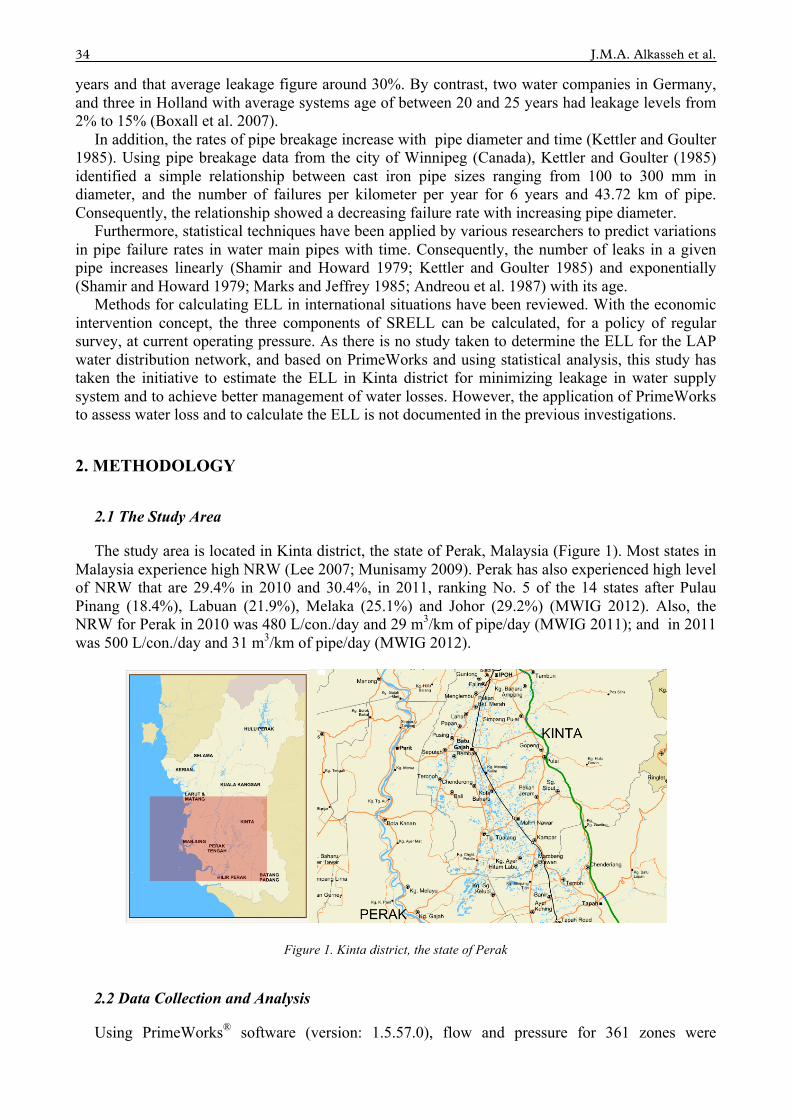
The study area is located in Kinta district, the state of Perak, Malaysia (Figure 1). Most states in Malaysia experience high NRW (Lee 2007; Munisamy 2009). Perak has also experienced high level of NRW that are 29.4% in 2010 and 30.4%, in 2011, ranking No. 5 of the 14 states after Pulau Pinang (18.4%), Labuan (21.9%), Melaka (25.1%) and Johor (29.2%) (MWIG 2012). Also, the NRW for Perak in 2010 was 480 L/con./day and 29 m3/km of pipe/day (MWIG 2011); and in 2011 was 500 L/con./day and 31 m3/km of pipe/day (MWIG 2012).

Figure 1. Kinta district, the state of Perak

2.2 Data Collection and Analysis

Using PrimeWorks® software (version: 1.5.57.0), flow and pressure for 361 zones were


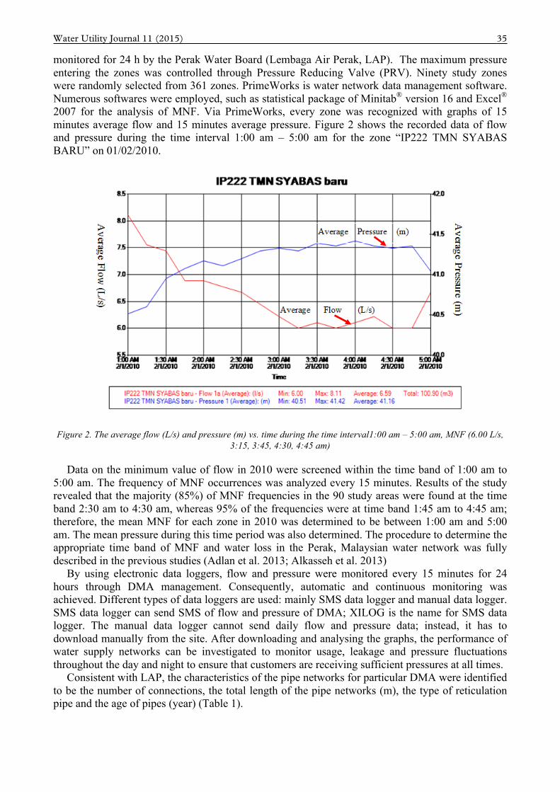
monitored for 24 h by the Perak Water Board (Lembaga Air Perak, LAP). The maximum pressure entering the zones was controlled through Pressure Reducing Valve (PRV). Ninety study zones were randomly selected from 361 zones. PrimeWorks is water network data management software. Numerous softwares were employed, such as statistical package of Minitab® version 16 and Excel® 2007 for the analysis of MNF. Via PrimeWorks, every zone was recognized with graphs of 15 minutes average flow and 15 minutes average pressure. Figure 2 shows the recorded data of flow and pressure during the time interval 1:00 am – 5:00 am for the zone “IP222 TMN SYABAS BARU” on 01/02/2010.

Figure 2. The average flow (L/s) and pressure (m) vs. time during the time interval1:00 am – 5:00 am, MNF (6.00 L/s, 3:15, 3:45, 4:30, 4:45 am)

Data on the minimum value of flow in 2010 were screened within the time band of 1:00 am to 5:00 am. The frequency of MNF occurrences was analyzed every 15 minutes. Results of the study revealed that the majority (85%) of MNF frequencies in the 90 study areas were found at the time band 2:30 am to 4:30 am, whereas 95% of the frequencies were at time band 1:45 am to 4:45 am; therefore, the mean MNF for each zone in 2010 was determined to be between 1:00 am and 5:00 am. The mean pressure during this time period was also determined. The procedure to determine the appropriate time band of MNF and water loss in the Perak, Malaysian water network was fully described in the previous studies (Adlan et al. 2013; Alkasseh et al. 2013)

By using electronic data loggers, flow and pressure were monitored every 15 minutes for 24 hours through DMA management. Consequently, automatic and continuous monitoring was achieved. Different types of data loggers are used: mainly SMS data logger and manual data logger. SMS data logger can send SMS of flow and pressure of DMA; XILOG is the name for SMS data logger. The manual data logger cannot send daily flow and pressure data; instead, it has to download manually from the site. After downloading and analysing the graphs, the performance of water supply networks can be investigated to monitor usage, leakage and pressure fluctuations throughout the day and night to ensure that customers are receiving sufficient pressures at all times.

Consistent with LAP, the characteristics of the pipe networks for particular DMA were identified to be the number of connections, the total length of the pipe networks (m), the type of reticulation pipe and the age of pipes (year) (Table 1).


Table 1. Characteristic of pipe networks for the zone IP222 TMN SYABAS BARU

Name of zone No. of Connection

Total length of pipe networks

(m)

Type of reticulation pipe

Age of pipes

(years) IP222 TMN SYABAS BARU 1,000 4,923 150mm AC 33

137 150mm DI 10

1,456 155mm uPVC 10

434 200mm uPVC 20

1,100 250mm MS 33

235 250mm AC 26 While each pipe in the network has different ages, the term weighted mean is the appropriate

estimate of the mean age of a particular zone (McKenzie and Lambert 2002; Spatz 2010; Alkasseh et al. 2013). For example, the weighted mean age of pipes for the zone IP222 TMN SYABAS BARU is 27.7 year:

Weighted mean age of pipes (year) = ∑=

∑=n

1iLengthi

n

1iAgei*Lengthi (1)

= 4,923 ∗ 33 + 137 ∗ 10 + 1,456 ∗ 10 + 434 ∗ 20 + 1,100 ∗ 33 + 235 ∗ 26

4,923 + 137 + 1,456 + 434 + 1,100 + 235 = 27.7 year

Further, correlation and regression techniques were used to determine interactions of variables.

Correlation (r) provides a unitless measure of association (usually linear) between two numerical measurements made on the same set of subjects and it is represented by correlation coefficient, whereas regression provides a means of predicting one variable (dependent variable) from the other (predictor variable) (Azman et al. 2006; Karthikeyan et al. 2013; Perugu et al. 2013).

2.2.1 Calculation of the economic volume for reported leaks and bursts

According to LAP, the recorded maintenance data include the quantities of water lost per pipe bursts, pipe size of each type of pipe and the location of maintenance. An example of the recorded frequency of repairs of the study zone IP 64 Tmn. Pinji Mewah is presented in Table 2.

Table 2. Frequency of repairs

Zone Code

Zone Name

Date of Complaints

Date of Completed

Type of Pipe

Pipe Size

Type of Leakage Comments

Estimate Loss of

Water (m3)

IP 64 Tmn. Pinji Mewah 31/03/10 09/04/10 GI pipe 20mm Service pipe Corrosion

pipe (hole) 69.12

IP 64 Tmn. Pinji Mewah 31/03/10 09/04/10 GI pipe 20mm Service pipe Corrosion

pipe (hole) 69.12

IP 64 Tmn. Pinji Mewah 31/03/10 19/04/10 HDPE

pipes 25mm Service pipe wound pipes 112.32

IP 64 Tmn. Pinji Mewah 22/06/10 24/06/10 150mm valve block service valve 23.33

IP 64 Tmn. Pinji Mewah 22/06/10 26/06/10 100mm valve block wear rubber 28.51

IP 64 Tmn. Pinji Mewah 22/06/10 23/06/10 HDPE

pipes 25mm Service pipe wound pipes 34.56

Firstly, for main pipe burst, the estimated water loss can be calculated using PrimeWorks

software. The actual amount can be determined by using the following equation:


Water loss = Area of graph during pipe burst (2)

When the pipe burst occurs, the flow jumps up, as can be seen from Figure 3. The latter showed that there was a pipe burst on 3rd July 2012 in the DMA IP 131 KG BARU KUALA KUANG. By zooming to the time of the event, the area of the pipe burst can be calculated, as shown in Figure 4.

Using the same time interval, the total amount of water on 3rd July 2012 will be compared to 2nd July 2012, as shown in Figure 5.

Figure 3. Pipe burst on 3rd July 2012

Figure 4. The exact time of pipe burst (3:30 am – 10:15 am)

From Figure 4, the exact time of the pipe burst is between 3:30 am and 10:15 am, approximately 6 hours and 45 minutes. The total amount of water consumption (loss + consumption) was 1118.36 m3. To get only the amount of water loss, the total amount of water consumption in this time interval will be compared to the previous day (2nd July 2012) using the same time interval. For example, the total amount of water consumption in the same time interval (3:30 am – 10:15 am) in


2nd July 2012 is 529.85 m3. Hence the amount of water loss during the pipe burst is 1118.36 m3 minus 529.85 m3 which is equal to 589 m3.

Figure 5. The total amount of water in 2nd July 2012 (3:30 am – 10:15 am)

According to LAP, the water loss for the service pipe can be calculated using the following equation:

Water loss = [time] X [leakage] (3)

Time = A + B, where A is the time between complain and repair, and B is the time of awareness B = [C or D], where C is the manual data logger (7 days) and D is SMS data logger (1 day) Leakage = K, where K (m3/day) is the water loss which is determined based on the studies on site.

2.2.2 Calculation of the economic volume for background leakage

The coefficients for unavoidable annual real loss (UARL) are suggested by IWA at 1999 which are based on length of main, number of service connection, length of pipe on private land, and pressure (Hyun et al. 2012). Hence, Background (undetectable) leakage is calculated using the relevant UARL parameters– 20 l/km mains/hr and 1.25 l/service connection/hr at 50m pressure. These are then adjusted for actual average pressure using FAVAD concepts with N1 exponent of 1.5 (Lambert and Lalonde 2005; Fanner and Lambert 2009).

Leakage varies with pressure (PN1): ⎟⎟⎠

⎞⎜⎜⎝

⎛=

p

P

LL

N

0

1

1

0

1 (4)

2.2.3 Calculation of the economic volume for unreported leaks and bursts

Methods of locating leaks vary from simple (listening on hydrants) to complex (noise loggers and night flow measurements), and have different costs (Muñoz-Trochez et al. 2010).

Figure 6 shows how the night flow in part of a distribution system (DMA IP222 TMN SYABAS BARU) in 2010 can gradually increase with time, because of ‘unreported’ leaks and bursts.


Figure 6. RR of unreported leakage for the DMA IP222 TMN SYABAS BARU

The economic unreported real losses (EURL) and other economic intervention parameters are calculated using a set of equations based on cost of intervention (CI), variable cost of water (CV), and rate of rise of unreported leakage (RR) (Lambert and Fantozzi 2005; Lambert and Lalonde 2005; Fantozzi and Lambert 2007; AWWA 2009).

If intervention cost (CI) is in RM (Ringgit Malaysia), variable cost (CV) is in RM/m3, and RR is in m3/day, per year, then:

Economic intervention frequency (EIF):

EIF (months) = (0.789 x CI/( S x CV))0.5 (5)

Economic percentage of system (EP):

EP% = 100 x (12/ EIF (months)) (6)

The annual budget for intervention (ABI):

ABI (RM) (excluding repair costs) = EP% x CI (7)

Economic annual volume of unreported real losses (EAVURL):

EAVURL (m3) = ABI/CV = EP x CI/CV (8)

For calculating each of the above parameters, it can be noted that the calculations of EIF, EP% and EAVURL are not highly sensitive to moderate random errors in CI, CV and S, due to the 0.5 exponent, and are independent of the currency units used, due to the use of ratio CI/CV (Lambert and Fantozzi 2005; Lambert and Lalonde 2005; Fanner and Lambert 2009).

2.2.4 LAP experience with economic intervention frequency

According to LAP, economic intervention frequency is equal to 1 time/zone/year. The zones are categorized into 2 types; active zones and passive (safe) zones. They do only detection for the active zones (priority). As for the safe zones, they seldom do leak detection. The basic indicator to determine the active and passive zone is by using the MNF. By doing that kind of monitoring, they are able to go to the zone and do leak detection. Usually, they are using the mechanical listening to carry out the detection. As for advance detection, they used the noise logger.


3. RESULTS AND DISCUSSION

3.1 Calculation of the economic volume for reported leaks and bursts

Based on LAP recorded frequency of repairs, Table 3 summarizes the frequency of repairs for each type of leakage in the ninety DMAs in 2010 including pipe repairs of main and service pipe, and the estimated water loss (m3) for main and service pipes. Table 4 shows the annual volume of water loss through the reported bursts and the estimated water loss per event for reported main burst and for service pipe.

Table 3. The estimated water loss (m3) for main and service pipes

Infrastructure components Burst No. (number) Estimated water loss (m3)

Main pipe 64 24,067.584 Service pipe 1312 58,854.412

Total 1376 82,922.00

Table 4. The annual volume of water loss through the reported bursts

Infrastructure components

Length or number

Burst No. (number)

Estimated water loss per year (m3)

Average rate per event (m3)

m3/h for 1 day

Main pipe (km) 644 64 24,067.584 376.06 15.67 Service pipe 71,185 1312 58,854.412 44.86 1.87

Total 1376 82,922.00 Loss/year from reported bursts = 3.19 l/connection/day* = 0.35 m3/km main/day**

*Loss/year from reported bursts = 82,922/71,185/365days x1000 = 3.19 l/connection/day **Loss/year from reported bursts = 82,922/644/365days = 0.35 m3/km main/day

From Table 4, the estimated water loss per event for reported main burst is about 376.06 m3

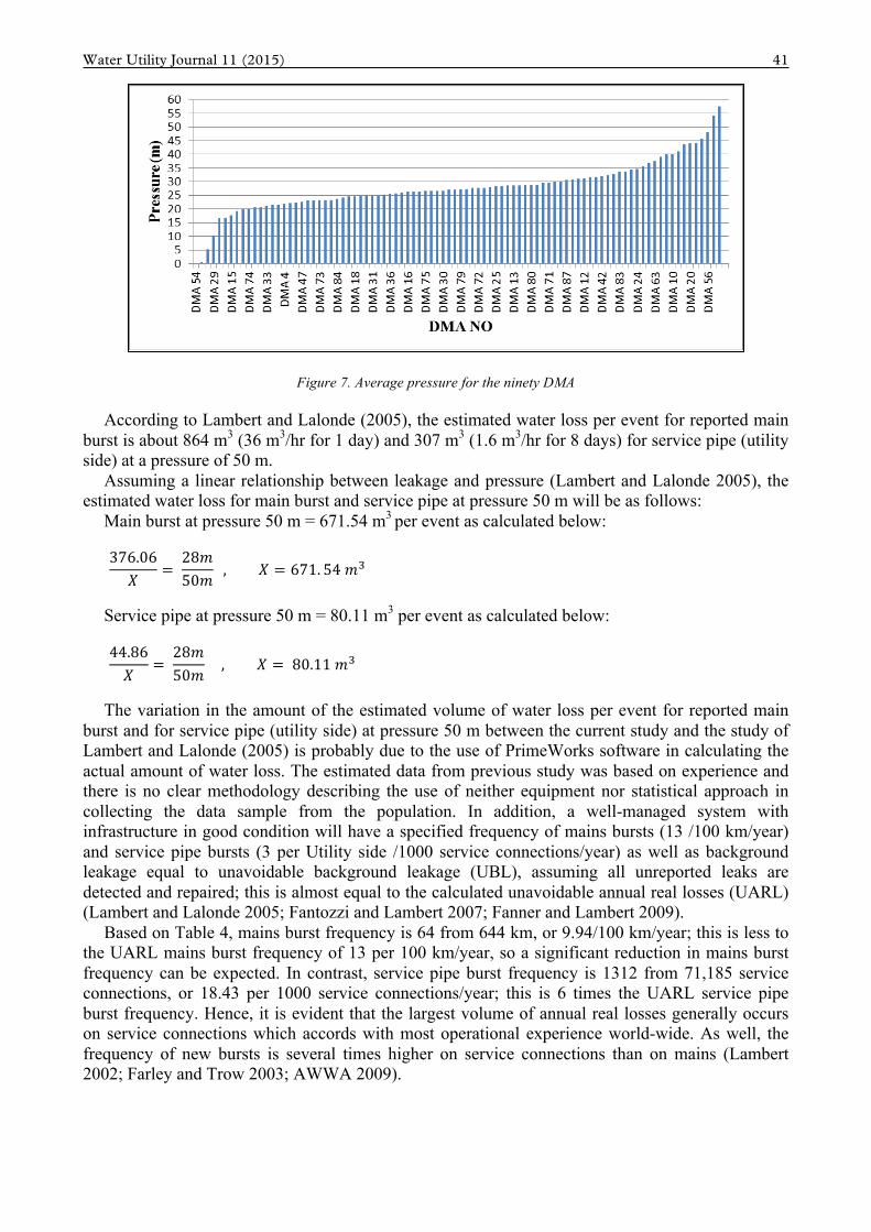
(15.67 m3/h for 1 day) and 44.86 m3 (1.87 m3/h for 1 day) for reported service pipe. Table 5 exhibits the descriptive statistics of the ninety DMAs including the average pressure for the 90 zones which is about 28 m. By referring to Figure 7, the majority of the DMAs (65.6%) have pressure less than or equal to 28 m. Using a significance level of α = 0.05, the correlation between test variables and MNF (l/s) of the 90 zones were carried out. Consequently, the output of the correlation test shows that the relationship between pressure (r = 0.107, p value, 0.315) and the MNF (l/s) was not significant. Also, the results of the correlation test indicate a significant linear relationship between the number of connections (r=0.488, p value < 0.001), reticulation length (r = 0.584, p value < 0.001), weighted mean age of pipe (r = 0.395, p value < 0.001), and MNF (l/s).

Currently, the most effective tools for leakage control in DMAs is the implementation of pressure management, particularly in large networks and in systems with deteriorated infrastructures and with high pressure (Gomes et al. 2012). Also, DMAs allowed a more efficient pressure management with a reduction of average system pressure of up to 20% (Fantozzi et al. 2009). Pressure management may be accomplished by installation of flow control or pressure reducing valves (Nicolini and Zovatto 2009).

Table 5. The descriptive statistics of the ninety DMAs

Descriptive Statistics: MNFmean (L/s), Connection No, Reticulation, ...

Variable N N* Mean Minimum Maximum MNFmean (L/s) 90 0 4.703 0.640 14.590 Connection NO. 90 0 790.9 29.0 3923.0 Reticulation Length (m) 90 0 7152 2310 19790 Weighted Mean of Age (ye 90 0 26.46 4.00 112.00 Pressure (m) 90 0 28.005 0.060 57.480


Figure 7. Average pressure for the ninety DMA

According to Lambert and Lalonde (2005), the estimated water loss per event for reported main burst is about 864 m3 (36 m3/hr for 1 day) and 307 m3 (1.6 m3/hr for 8 days) for service pipe (utility side) at a pressure of 50 m.

Assuming a linear relationship between leakage and pressure (Lambert and Lalonde 2005), the estimated water loss for main burst and service pipe at pressure 50 m will be as follows:

Main burst at pressure 50 m = 671.54 m3 per event as calculated below:

376.06𝑋

= 28𝑚50𝑚

, 𝑋 = 671. 54 𝑚!

Service pipe at pressure 50 m = 80.11 m3 per event as calculated below:

44.86𝑋

= 28𝑚50𝑚

, 𝑋 = 80.11 𝑚!

The variation in the amount of the estimated volume of water loss per event for reported main burst and for service pipe (utility side) at pressure 50 m between the current study and the study of Lambert and Lalonde (2005) is probably due to the use of PrimeWorks software in calculating the actual amount of water loss. The estimated data from previous study was based on experience and there is no clear methodology describing the use of neither equipment nor statistical approach in collecting the data sample from the population. In addition, a well-managed system with infrastructure in good condition will have a specified frequency of mains bursts (13 /100 km/year) and service pipe bursts (3 per Utility side /1000 service connections/year) as well as background leakage equal to unavoidable background leakage (UBL), assuming all unreported leaks are detected and repaired; this is almost equal to the calculated unavoidable annual real losses (UARL) (Lambert and Lalonde 2005; Fantozzi and Lambert 2007; Fanner and Lambert 2009).

Based on Table 4, mains burst frequency is 64 from 644 km, or 9.94/100 km/year; this is less to the UARL mains burst frequency of 13 per 100 km/year, so a significant reduction in mains burst frequency can be expected. In contrast, service pipe burst frequency is 1312 from 71,185 service connections, or 18.43 per 1000 service connections/year; this is 6 times the UARL service pipe burst frequency. Hence, it is evident that the largest volume of annual real losses generally occurs on service connections which accords with most operational experience world-wide. As well, the frequency of new bursts is several times higher on service connections than on mains (Lambert 2002; Farley and Trow 2003; AWWA 2009).


3.2 Calculation of the economic volume for background leakage

Average zone pressure (AZP) and average night zone pressure (ANZP) are often used to calculate the UARL (Muñoz-Trochez et al. 2010). To demonstrate the effect of introducing pressure options to SRELL calculations, the background leakage at the new average pressure (28 metres) can be calculated using the FAVAD equation with an exponent of 1.5, and using the relevant UARL parameters – 20 l/km mains/hr and 1.25 l/service connection/hr at 50m pressure (Lambert and Lalonde 2005; Fantozzi and Lambert 2007; Fanner and Lambert 2009), as shown in Table 6. The coefficients for UARL are suggested by IWA at 1999 (Hyun et al. 2012).

Table 6. Calculation of unavoidable background leakage at current pressure


Length or

number @50 m pressure

@50 m pressure m3/day

@28 m pressure m3/day

@28 m pressure m3/year

Main pipe (km) 644 20 l/km mains/hr 309.12 129.54 47,282.67

Service pipe 71,185 1.25 l/service connection/hr 2135.55 894.94 326,651.49

Total 2,444.67 1,024.48 373,934.17 Unavoidable background

leakage =14.39 l/connection/day* = 1.59 m3/km main/day**

* Unavoidable background leakage = (374000/71185/365) x1000 = 14.39 l/connection/day ** Unavoidable background leakage = 374000/644/365 = 1.59 m3/km main/day

L varies with PN1 and ⎟⎟⎠

⎞⎜⎜⎝

⎛=

p

P

LL

N

0

1

1

0

1

Unavoidable background leakage at current pressure (28 m) for main pipe:

!!"#.!"

= !"!"

!.!, 𝑋 = 129.54 𝑚! /𝑑𝑎𝑦

Unavoidable background leakage at current pressure (28 m) for service pipe:

X2135.55

= 2850

!.!, 𝑋 = 894.94 𝑚! /𝑑𝑎𝑦

Based on BABE methodology, the background leakage has a lower flow rate and is a function of the condition of the network infrastructure. The infrastructure condition factor (ICF) can have a value from 0.5, that means the infrastructure is in good condition, to 2.0, which means the water tightness in the pipes is very poor (Farley 2001). In the present study, there is no reliable information about ICF, so a value of 1.0 is chosen based on the recommendation of Farley (2001). The ICF – the multiplier for UBL is used to adjust the calculated UBL to a value consistent with the leakage remaining immediately after a leak detection intervention & repairs (Lambert and Lalonde 2005). From Table 6, it is evident that the large number of joints and fittings on service connections between the main and the street boundary result in a relatively high value for background leakage in this part of the infrastructure (Lambert 2002; Farley and Trow 2003).

3.3 Calculation of the economic volume for unreported leaks and bursts

Figure 8 illustrates the natural rate of rise of unreported leakage for ninety DMAs.


120100806040200

1400

1200

1000

800

600

400

200

0

Weighted Mean of Age (year)

MNF

mea

n (m

3/da

y)

S 251.562R-Sq 15.6%R-Sq(adj) 14.6%

Fitted Line PlotMNFmean (m3/day) = 200.9 + 7.762 Weighted Mean of Age (year)

Figure 8. RR of unreported leakage for ninety DMAs

Using a significance level of α = 0.05, the outputs of the regression analysis (MNFmean (m3/day) vs. weighted mean of age (year)) of RR of unreported leakage for ninety DMAs are shown in Table 7. The R-square value was 0.156. This value shows that 15.6 % of the variation in the MNF mean (m3/day) could be explained by the model. The adjusted R-square is 0.146. At 5 % significance level, F-value for the model was 16.26. The p value was less than 0.001. Thus, the above regression model was statistically significant. Consequently, the RR for the ninety DMAs is 7.762 m3/day/year. Based on night flow measurements, RR for a small district in Northern Italy (900 service connections; 16 km of mains) was 80.4 m³/day/Year (Lambert and Fantozzi 2005). For an Australian System (16,000 service connections; 603 km of mains), RR was 320 m3/day/year (Lambert and Lalonde 2005).

Table 7. RR of unreported leakage for ninety DMAs: MNFmean (m3/day) vs. weighted mean of age (year)

The marginal (or unit) cost of water is derived by dividing total operating and maintenance costs,

in terms of power, chemicals and possibly labour, by total production (Pearson and Trow 2005; Lee 2007). According to MWIG (2011), Operating Expenditure/Total Production in 2009 and 2010 in Perak was RM 0.37 /m3.

All parameters for economic intervention are as follows: § Rate of rise (RR) = 7.762 m3/day/year.

Regression Analysis: MNFmean (m3/day) versus Weighted Mean of Age (year)

The regression equation is MNFmean (m3/day) = 200.9 + 7.762 Weighted Mean of Age (year) S = 251.562 R-Sq = 15.6% R-Sq(adj) = 14.6% Analysis of Variance Source DF SS MS F P Regression 1 1028851 1028851 16.26 0.000 Error 88 5568930 63283 Total 89 6597781


§ Intervention cost (CI) using noise loggers = € 4,000 (Lambert and Fantozzi 2005) = RM 15,914.24 according to Exchange Currency Converter 2013, as shown in Figure 9.

§ Variable cost of water (CV) = RM 0.37 /m3 (MWIG 2011).

Figure 9. Exchange Rates: Euro↔Malaysian Ringgit

Calculations of the economic unreported real losses (EURL) and other economic intervention parameters for regular survey are as follows:

Economic frequency of intervention (EIF):

EIF (months)=(0.789 x CI/( S x CV))0.5= (0.789x 15,914.24 /(7.762x0.37))0.5=66.122 months ≈ 66 months

Economic Percentage of System (EP):

EP% = 100 x (12/ EIF (months)) = 100x(12/66) = 18% of system each year

The Annual Budget for Intervention (ABI):

ABI (RM) (excluding repair costs) = EP% x CI = 0.18x RM 15,914.24 = RM 2,864.56/year

Economic annual volume of unreported real losses (EAVURL):

EAVURL (m3) = ABI/V = EP x CI/CV = 0.18x RM 15,914.24/0.37 = 7,742.06 m3/year

The appropriate level of intervention to manage unreported real losses can be evaluated in terms of how frequent leak survey are economically effective which is proportional to the cost of leak survey (CI) and inversely proportional to the variable cost of real losses; the higher the cost of water, the shorter the survey frequency. The economic frequency of intervention is also inversely proportional to the rate of rise of unreported leakage from year to year (RR); the more rapid the increase in unreported leakage between surveys, the shorter the frequency (AWWA 2009). Global experiences (German DVGW) recommend intervention from once/year to once/6 years, depending upon leakage level. In England & Wales, companies intervene from 3 times per year to every 3 years in individual districts and AWWA M36 Manual suggests that on average it is economic to intervene every 4 years (Lambert and Lalonde 2005). For large systems, it is preferable to intervene in an appropriate percentage of the system each year, rather than to wait and then intervene in the whole system once every few years (Lambert and Fantozzi 2005; Wyatt 2010).

The economic intervention calculations indicate that the economic frequency of leak survey and repair intervention is around 66 months (5.5 year), and target around 18% of the system to be checked each year. Hence, it is preferable to structure leak survey efforts to cover 18 % of the system each year rather than doing the entire system every 5.5 years.

3.4 Summary of the ELL calculations

Assuming a basic active leakage control policy of regular survey, the SRELL calculations at current operating pressure for the present system are summarised in Table 8. Results of the study revealed that SRELL will be around 17.88 l/service connection/day or 2.0 m3/km mains/day.


Table 8. Summary of ELL calculations, assuming regular survey

Assumed FAVAD N1 for Reported Bursts = 1.0 Assumed FAVAD N1 for Background Leakage = 1.5


Length or number

Real Losses from reported

bursts m3/year

Unavoidable background

leakage m3/year

Economic unreported real losses m3/year

Short -Run Economic Leakage Level SRELL

m3/year

Main pipe (km) 644 24,067.584 47,282.67 7,742.06 464,598.23 Service pipe 71,185 58,854.412 326,651.49 Total 82,922.00 373,934.17 7,742.06 464,598.23

SRELL = 17.88 l/service connection /day 2.0 m3/km mains/day

4. CONCLUSIONS

Many utilities have developed strategies to reduce water losses to an economic or acceptable level. For a policy of regular survey, at current operating pressure, the three components of short-run economic leakage level (SRELL) can be calculated using the economic intervention concept. Thereupon, the real losses from reported bursts are estimated from a number of reported burst repairs using PrimeWorks software (3.19 l/connection/day, 0.35 m3/km main/day); background (undetectable) leakage is evaluated as a multiple of unavoidable background leakage (14.39 l/connection/day, 1.59 m3/km main/day) as well as economic annual volume of unreported real losses is determined using economic intervention theory and regression analysis (7,742.06 m3/year). Consequently, short-run economic leakage level (SRELL) in the Perak, Malaysian water network will be around 17.88 l/service connection /day or 2.0 m3/km mains/day. In conclusion, an acceptable study for calculating ELL should be integrated with PrimeWorks for effective assessment and management of NRW and its components.

ACKNOWLEDGMENTS

The authors are very grateful to the Perak Water Board (Lembaga Air Perak, LAP) for their support and providing the required data for this study and in particular Ministry of Higher Education Malaysia for providing LRGS Grant No. 203/PKT/6726001 - River bank/bed Filtration for Drinking Water Source Abstraction to fund this research. The authors would like to particularly thank the Institute of Postgraduate Studies, Universiti Sains Malaysia, for their valuable assistance.

REFERENCES

Adlan MN, Alkasseh JM, Abustan HI, Hanif ABM (2013) Identifying the appropriate time band to determine the minimum night flow: a case study in Kinta Valley, Malaysia. Water Sci Technol Water Supply 13 (2) 328-336.

Alkasseh JM, Adlan MN, Abustan I, Aziz HA, Hanif ABM (2013) Applying Minimum Night Flow to Estimate Water Loss Using Statistical Modeling: A Case Study in Kinta Valley, Malaysia. Water Resour Manage 27 (5) 1439-1455.

Andreou SA, Marks DH, Clark RM (1987) A new methodology for modelling break failure patterns in deteriorating water distribution systems: Theory. Adv Water Res 10 (1) 2-10.

AWWA (2009) Water Audits and Loss Control Programs. 3rd Edition of Manual of Water Supply Practices M36, American Water Works Association, Denver, USA.

Azman J, Frković V, Bilić-Zulle L, Petrovecki M (2006) Correlation and regression. Acta medica Croatica: c̆asopis Hravatske akademije medicinskih znanosti 60 (1) 81-91.

Beuken R, Lavooij C, Bosch A, Schaap P (2006) Low leakage in the Netherlands confirmed. in Proceedings of the 8th Annual Water Distribution Systems Analysis Symposium ASCE, Cincinnati, USA.

Boxall J, O'hagan A, Pooladsaz S, Saul A, Unwin D (2007) Estimation of burst rates in water distribution mains. in Proceedings of the Institution of Civil Engineers-Water Management, London:[Published for the Institution of Civil Engineers by Thomas Telford Ltd.], c2004-, Department of Probability and Statistics and Department of Civil and Structural Engineering, University of Sheffield, Sheffield, England, pp. 73-82.

Çakmakcı M, Uyak V, Öztürk İ, Aydın AF, Soyer E, Akça L (2007) The Dimension and Significance of Water Losses in Turkey. in Proceedings of IWA Specialist Conference on Water Loss, , Bucharest, Romania,, pp. 464-473.


Cannarozzo M, Criminisi A, Gagliardi M, Mazzola MR (2006) Statistical Analysis of Water Main Failures in the Distribution Network of an Italian Municipality. in 8th Annual Water Distribution Systems Analysis Symposium, , ASCE, Cincinnati, Ohio, USA, pp. 1-18.

Cheung PB, Girol GV, Abe N, Propato M (2010) Night flow analysis and modeling for leakage estimation in a water distribution system. Integrating Water Systems–Maksimovic, Taylor & Francis Group 509-513.

Covas D, Jacob A, Ramos H (2006) Bottom-Up Analysis for Assessing Water Losses: A Case Study. in 8th Annual Water Distribution Systems Analysis Symposium, ASCE, Cincinnati, Ohio, USA, pp. 1-19.

Crowder GS, Hassan SMS, Lee MK (2012) Developing the Network Improvement Plan for Selangor State, Malaysia. in Procceedings of the 7th IWA Water Loss Reduction Specialist Conference, Manila, Philippines, pp. 1-7.

Di Nardo A, Di Natale M, Santonastaso GF, Venticinque S (2013) An Automated Tool for Smart Water Network Partitioning. Water Resour Manage 27 (13) 4493–4508.

Fanner P, Lambert AO (2009) Calculating SRELL with pressure management, active leakage control and leak run-time options, with confidence limits. in Proceedings of 5th IWA Water Loss Reduction Specialist Conference, Cape Town, South Africa: IWA/Specialist Group Efficient Operation and Management., pp. 373–380.

Fantozzi M, Calza F, Lambert A (2009) Experience and results achieved in introducing District Metered Areas (DMA) and Pressure Management Areas (PMA) at Enia utility (Italy). In Water Loss Specialist Conference, International Water Association, Cape Town, South Africa.

Fantozzi M, Lambert A (2007) Including the effects of pressure management in calculations of Short-Run Economic Leakage Levels. in Proceedings of IWA Specialist Conference Water Loss, Bucharest, Romania.

Fantozzi M, Lambert AO (2010) Recent Developments in Pressure Management. in Presented to International Water Loss Conference, Sao Paolo, Brazil.

Farley M (2001) Leakage management and control - A best practice training manual, World Health Organization, Geneva, Switzerland.

Farley M, Trow S (2003) Losses in Water Distribution Networks; A practitioner’s Guide to Assessment, Monitoring and Control., IWA Publishing,, London, UK.

García VJ, Cabrera E, Enrique Cabrera J (2006) The Minimum Night Flow Method Revisited. in 8th Annual Water Distribution Systems Analysis Symposium, ASCE, Cincinnati, Ohio, USA, pp. 1-18.

Girard M, Stewart RA (2007) Implementation of pressure and leakage management strategies on the Gold Coast, Australia: case study. J Water Resour Plann Manage 133(3) 210-217.

Gomes R, Marques AS, Sousa J (2012) Identification of the optimal entry points at District Metered Areas and implementation of pressure management. Urban Water J, Taylor & Francis, DOI:10.1080/1573062X.2012.682589.

Gomes R, Marques AS, Sousa J (2013) District Metered Areas Design Under Different Decision Makers’ Options: Cost Analysis. Water Resour Manage 27 (13) 4527–4543.

Hamilton S, Mckenzie R, Seago C (2006) A Review of Performance Indicators for Real Losses from Water Supply Systems. Voda i sanitarna tehnika 36 (6) 15-24.

Hyun I, Lee K, Dockko S, Choi S, Kim D (2012) A method to determine the average water pressure for the calculation of the UARL. in Procceedings of the 7th IWA Water Loss Reduction Specialist Conference, Manila, Philippines, pp. 1-2.

Karadirek I, Kara S, Yilmaz G, Muhammetoglu A, Muhammetoglu H (2012) Implementation of hydraulic modelling for water-loss reduction through pressure management. Water Resour Manage 26 (9) 2555–2568.

Karthikeyan L, Kumar DN, Graillot D, Gaur S (2013) Prediction of Ground Water Levels in the Uplands of a Tropical Coastal Riparian Wetland using Artificial Neural Networks. Water Resour Manage 27 (3) 871-883.

Kettler AJ, Goulter IC (1985) An analysis of pipe breakage in urban water distribution networks. Can J Civ Eng 12 (2) 286-293. Kingdom B, Liemberger R, Marin P (2006) The challenge of Reducing Non-Revenue Water (NRW) in Developing Countries, Water

Supply and Sanitation Sector Board Discussion Paper Series, Paper No.8. Lambert A (2002) International Report: Water lusses management and techniques. Water Sci Technol Water Supply 1-20. Lambert A, Fantozzi M (2005) Recent advances in calculating economic intervention frequency for active leakage control, and

implications for calculation of economic leakage levels. Water Sci Technol Water Supply 5 (6) 263. Lambert A, Lalonde A (2005) Using practical predictions of Economic Intervention Frequency to calculate Short-run Economic

Leakage Level, with or without Pressure Management. in Proceedings of IWA Specialised Conference ‘Leakage 2005’, Halifax, Nova Scotia, Canada, pp. 310-321.

Lee C (2007) Social policies and private sector participation in water supply–the case of Malaysia. United Nations Research Institute for Social Develeopment (UNRISD).

Marks DH, Jeffrey LA (1985) Predicting urban water distribution maintenance strategies: A case study of New Haven, Connecticut. in Department of Civil Engineering, Massachusetts Institute of Technology, Department of Civil Engineering, USA.

Mckenzie R, Lambert A (2002) ECONOLEAK: economic model for leakage management for water suppliers in South Africa, User Guide. WRC Report TT 169/02, South Africa.

Morgan W (2006) Manager to Manager -- Managing Water Loss. J Am Water Works Assn 98 (2) 32-37. Mounce S, Boxall J, Machell J (2010) Development and verification of an online artificial intelligence system for detection of bursts

and other abnormal flows. J Water Resour Plann Manage 136(3) 309–318. Munisamy S (2009) Efficiency and ownership in water supply: Evidence from Malaysia. International Review of Business Research

Papers 5 (6) 148-260. Muñoz-Trochez C, Smout I, Kayaga S (2010) Incorporating energy use into the economic level of Leakage Model. in World Wide

Workshop for Young Environmental Scientists: 2010 proceedings, Arcueil : France. Mutikanga HE, Sharma SK, Vairavamoorthy K (2012) Review of Methods and Tools for Managing Losses in Water Distribution

Systems. J Water Resour Plann Manage. doi:10.1061/(ASCE)WR.1943-5452.0000245. MWIG (2011) Malaysia Water Industry Guide (2011). in, The Malaysian Water Association (MWA), Kuala Lumpur, Malaysia.


MWIG (2012) Malaysia Water Industry Guide (2012). in, The Malaysian Water Association (MWA), Kuala Lumpur, Malaysia. Nazif S, Karamouz M, Yousefi M, Zahmatkesh Z (2013) Increasing Water Security: An Algorithm to Improve Water Distribution

Performance. Water Resour Manage 27 (8) 2903–2921. Nicolini M, Zovatto L (2009) Optimal location and control of pressure reducing valves in water networks. J Water Resour Plann

Manage 135 178-187. Öztürk İ, Uyak V, Çakmakci M, Akça L (2007) Dimension of water loss through distribution system and reduction methods in

Turkey. in International Congress on River Basin Management, pp. 245-255. Pearson D, Trow S (2005) Calculating the Economic Levels of Leakage. in Proceedings of IWA Specialised Conference 'Leakage

2005', Halifax, Nova Scotia, Canada, pp. 294-309. Perugu M, Singam AJ, Kamasani CSR (2013) Multiple Linear Correlation Analysis of Daily Reference Evapotranspiration. Water

Resour Manage 27 (5) 1489–1500. Pickard BD, Vilagos J, Nestel GK, Fernandez R, Kuhr S, Lanning D (2008) Reducing Non-RevenueWater: A Myriad of Challenges.

FLA WATER RESOUR J 26-32. Puust R, Kapelan Z, Savic D, Koppel T (2010) A review of methods for leakage management in pipe networks. Urban Water J 7 (1)

25-45. Pyzoha DS (2013) An economical and sustainable alternative to open-cut construction for small-diameter water main rehabilitation. J

Am Water Works Assn 105 (7) 64-77. Shamir U, Howard CDD (1979) An analytic approach to scheduling pipe replacement. J Am Water Works Assn 71 (5) 248-258. Spatz C (2010) Basic Statistics: Tales of Distributions, Wadsworth, Cengage Learning, Belmont CA, USA. 487 pp. Stephens I (2003) Regulating Economic Levels of Leakage in England and Wales. in WORLD WATER WEEK, Office of water

(OFWAT), WASHINGTON, DC,. Tabesh M, Yekta Aha, Burrows R (2009) An integrated model to evaluate losses in water distribution systems. Water Resour

Manage 23 (3) 477-492. Thornton J, Lambert A (2007) Pressure management extends infrastructure life and reduces unnecessary energy costs. in Proceedings

of IWA Special Conference 'Water Loss 2007, Bucharest, Romania, 23-27. Thornton J, Sturm R, Kunkel G (2008) Water loss control, McGraw-Hill New York, USA. Trow SW, Tooms S (2012) Deciding on the economic balance between Active Leakage Control and Pressure Management. in

Proceedings of the 7th IWA Water Loss Reduction Specialist Conference, Manila, Philippines, 1-9. Williams P (2013) Information engineering: An integrated approach to water system management. J Am Water Works Assn 105 (6)

61-66. Wyatt AS (2010) Non-Revenue Water: Financial Model for Optimal Management in Developing Countries. RTI Press publication

MR-0018-1006.

achieving an economic leakage level in kinta valley, · pdf fileachieving an economic leakage...

Documents