advance process control i carlos velázquez pharmaceutical engineering research laboratory erc on...
TRANSCRIPT

Advance Process Control I
Carlos VelázquezPharmaceutical Engineering Research Laboratory
ERC on Structured Organic Particulate SystemsDepartment of Chemical Engineering
University of Puerto Rico at Mayaguez

Process Control and Optimization
• Control and optimization are terms that are many times erroneously interchanged.
• Control has to do with adjusting flow rates to maintain the controlled variables of the process at specified setpoints.
• Optimization chooses the values for key setpoints such that the process operates at the “best” economic conditions.

Review of Basic Control

Conservation Equations:Mass, Moles, or Energy Balances
Systemthewithinaction
byGenerationofRate
Systemthe
LeavingRate
Systemthe
EnteringRate
onAccumulati
ofRate
Re
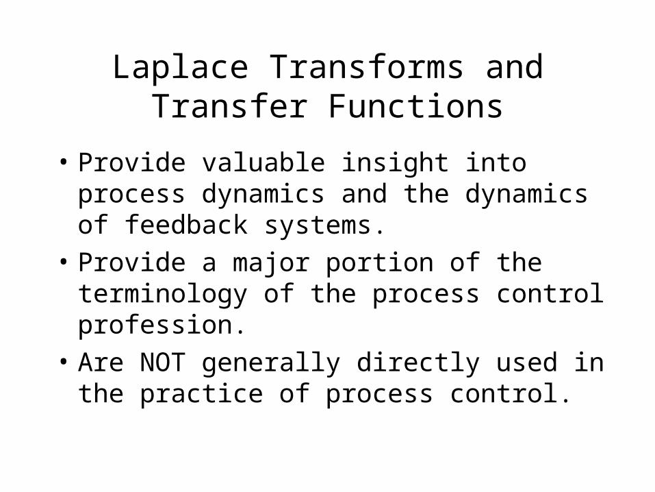
Laplace Transforms and Transfer Functions
• Provide valuable insight into process dynamics and the dynamics of feedback systems.
• Provide a major portion of the terminology of the process control profession.
• Are NOT generally directly used in the practice of process control.

Method for Solving Linear ODE’s using Laplace Transforms
Laplace Domain
Time Domain
dy/dt = f(t,y)
sY(s) - y(0) =F(s,Y)
Y(s) = H(s)
y(t) = h(t)

Transfer Functions
• Defined as G(s) = Y(s)/U(s)
• Represents a normalized model of a process, i.e., can be used with any input.
• Y(s) and U(s) are both written in deviation variable form.
• The form of the transfer function indicates the dynamic behavior of the process.

Example of Derivation of a Transfer Function
)()()()()(
212211 tTFFtTFtTFdt
tdTM • Dynamic model of
CST thermal mixer• Apply equation to the
steady state• Substitute deviation
variables• Equation in terms of
deviation variables.
0220110 TTTTTTTTT
)()(
)()()(
21
2211
tTFF
tTFtTFdt
tTdM
)0()()0()0()0(
212211 TFFTFTFdt
dTM

Derivation of a Transfer Function
21
1
1 )(
)()(
FFsM
F
sT
sTsG
• Apply Laplace transform to each term considering that only inlet and outlet temperatures change.
• Determine the transfer function for the effect of inlet temperature changes on the outlet temperature.
• Note that the response is first order.
21
2211 )()()(
FFsM
sTFsTFsT

What if the Process Model is Nonlinear
• Before transforming to the deviation variables, linearize the nonlinear equation.
• Transform to the deviation variables.
• Apply Laplace transform to each term in the equation.
• Collect terms and form the desired transfer functions.

Use Taylor Series Expansion to Linearize a Nonlinear Equation
...)()()(0
00
xxdx
dyxxxyxy
• This expression provides a linear approximation of y(x) about x=x0.
• The closer x is to x0, the more accurate this equation will be.
• The more nonlinear that the original equation is, the less accurate this approximation will be.
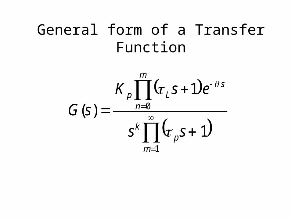
General form of a Transfer Function
1
0
1
1)(
mp
k
sm
nLp
ss
esKsG

Dynamic Modeling Approach for Process Control Systems
Actuator Process Sensorc y y su

Dynamic Model for Sensors• These equations
assume that the sensors behave as a first order process.
• The dynamic behavior of the sensor is described by the time constant since the gain is unity
• T and L are the actual temperature and level.
sTs
s TTdt
dT
1
sLs
s LLdt
dL
1

Dynamic Model for Sensors• The units of KT
depend on the input to the sensor and the type of signal of the sensor.
• For instance, if input is pressure and the signal from the sensor is in mA, then KT = psig/mA
1)(
s
KsH
T
T
• input : concentration,
level, pressure, temperature, force, velocity
• Signals : mA, mV, %TO

Actuator System
• Control Valve– Valve body– Valve actuator
• I/P converter
• Instrument air system

Dynamic Model for Actuators
FFdt
dFspec
v
1
QQdt
dQspec
H
1
• These equations assume that the actuator behaves as a first order process.
• The dynamic behavior of the actuator is described by the time constant since the gain is unity

Dynamic Response of an Actuator (First Order Process)
0 2 4 6 8 10Time (seconds)
Fspec
F
Parameter Estimation


Estimation of Transfer Functions
• Factors involved– Sampling time– Signal-to-noise ratio– Input type

1) Sampling time (T)
• If proper sampling is not used, the data could be corrupted by too much noise (fast sampling) or could lack of enough dynamic data (too slow sampling)
Figure 3.6 Effect of a double pulse and T= 10.0 in the SSE surface of a FO model
K
p
p

Figure 3.7 Effect of a double pulse and T= 100.0 in the SSE surface of a FO model
Kp
p

2) Signal-to-Noise ratio
• Measures how big is the signal of the measured variable compared to the signal of the noise

Figure 3.14 Effect of a double pulse and a S/N = 10:1 in the SSE surface of a FO model, T = 1.0
Kp
p

Figure 3.15 Effect of a double pulse and a S/N = 1:1 in the SSE surface of a FO model, T =1.0
Kp
p

3) Input wave form
• Virtually any type of input can be used. The amplitude of the signal is the key factor for an input to be proper.
0
1
step pulse
0
1
0
1
doublet
-1
0
1
sinusoidal
-1
0
1
PRBS
-1

Figure 3.1 Effect of a step change in the SSE surface of a FO model
Kp
p

Figure 3.2 Effect of a pulse in the SSE surface of a FO model
Kp
p
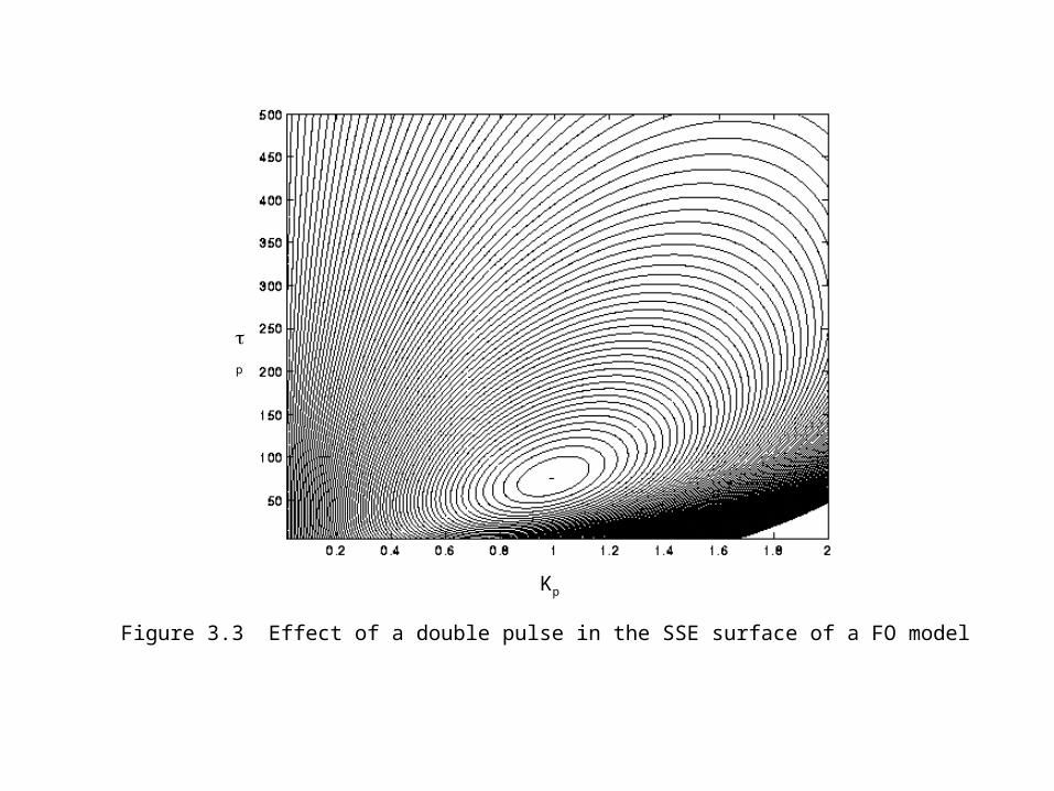
Figure 3.3 Effect of a double pulse in the SSE surface of a FO model
Kp
p

Figure 3.4 Effect of sinusoid in the SSE surface of a FO model
Kp
p
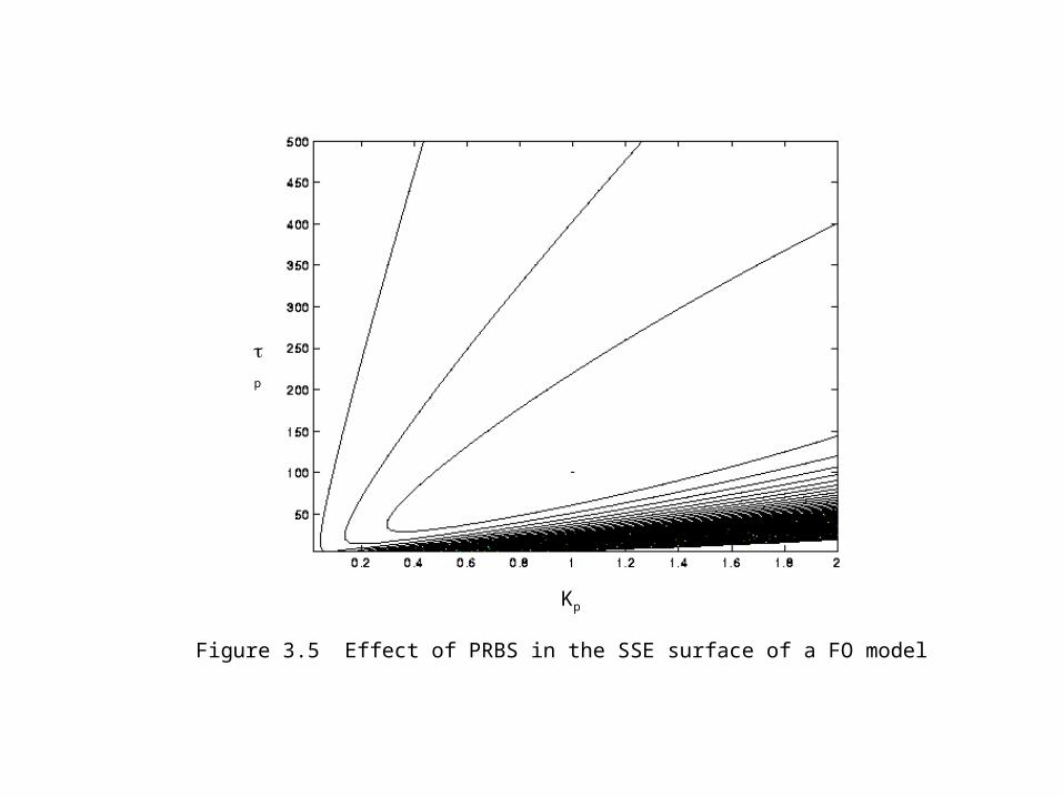
Figure 3.5 Effect of PRBS in the SSE surface of a FO model
Kp
p
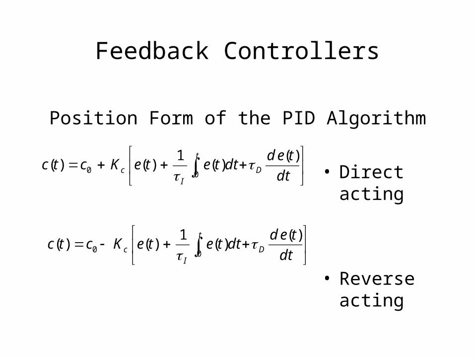
Feedback Controllers
• Direct acting
• Reverse acting
t
DI
c dt
teddtteteKctc
00
)()(
1)()(
t
DI
c dt
teddtteteKctc
00
)()(
1)()(
Position Form of the PID Algorithm

Definition of Terms
• e(t)- the error from setpoint [e(t)=ysp-ys].
• Kc- the controller gain is a tuning parameter and largely determines the controller aggressiveness.
• I- the reset time is a tuning parameter and determines the amount of integral action.
• D- the derivative time is a tuning parameter and determines the amount of derivative action.
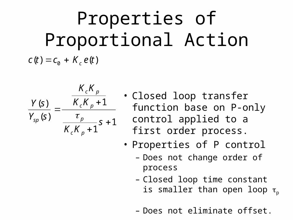
Properties of Proportional Action
11
1
)(
)(
)()( 0
sKK
KK
KK
sY
sY
teKctc
pc
p
pc
pc
sp
c
• Closed loop transfer function base on P-only control applied to a first order process.
• Properties of P control– Does not change order of process
– Closed loop time constant is smaller than open loop p
– Does not eliminate offset.

Offset Resulting from P-only Control
Time
Setpoint1.0
1
2
3
0
Offset

Properties of Integral Action
• Based on first order process
• Properties of I control– Offset is eliminated
– Increases the order by 1
– As integral action is increased, the process becomes faster, but at the expense of more sustained oscillations
pcp
I
pc
pII
pc
I
pc
pIsp
t
I
c
KK
KK
sKK
sKK
sY
sY
dtteK
ctc
2
1
1
1
)(
)(
)()(
2
00

Integral Action for the Response of a PI Controller
Time
ys
ysp

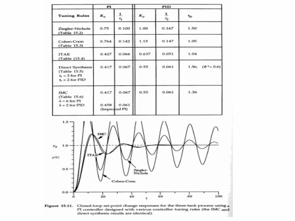
Controller Tuning
• Ziegler-Nichols
• Integral Criteria
• Internal Model Control
• Frequency Techniques

Stability
• Substitution
• Root Locus
• Frequency techniques

Stability of the Control Loop
• For a feedback control loop to be stable, all the roots of its characteristic equation must be either negative real numbers or complex numbers with negative real parts.

Stability of a Controlled System
• Method 1: Direct Substitution– Select a P-Only controller.
– Write the characteristic equation in a polynomial form of s.
– Substitute s=wui and Kc=Kcu
– Solve for Kcu and wu
01)()()()( sGsGsGsG cTpa
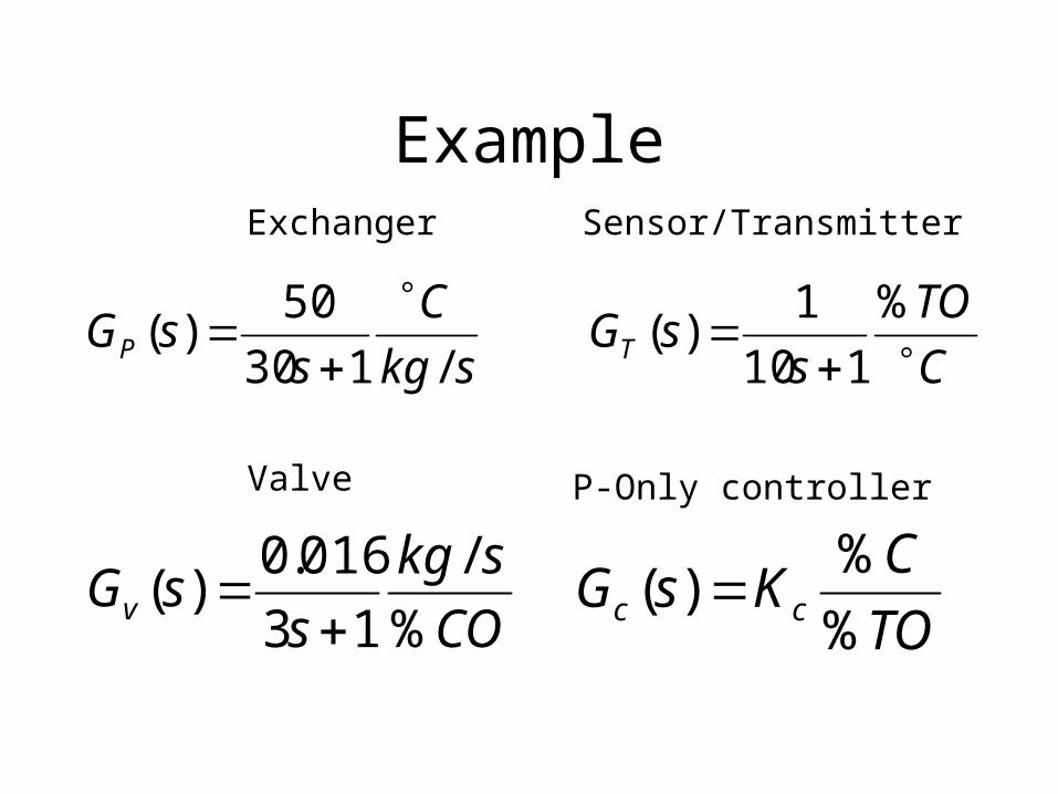
Example
skg
C
ssGP /130
50)(
C
TO
ssGT
%
110
1)(
CO
skg
ssGv %
/
13
016.0)(
TO
CKsG cc %
%)(
Exchanger Sensor/Transmitter
Valve P-Only controller

Solution
0)()()()(1 sGsGsGsG cTPv
013
016.0
130
50
110
11
cK
sss
08.0143420900 23 cKsss
08.0143420900 ,23 ucuuu Kiwiwiw
Characteristicequation
SubstitutingcorrespondingTFs
Rearranging
Substituting s=iwu, and Kc=Kcu

Solution
;%
%8.23/2186.0
;%
%25.10
043900
080.01420
;004390080.01420
3
2
32
TO
COKsradwFor
TO
COKwFor
K
iiK
cuu
cuu
uu
cuu
uucuu
ww
w
www
The real and imaginary parts have to be each one equal to zero to make the equation equal to zero.

Solution
• To determine the correct range, first we need to determine the sign of the multiplication of the gain of the process, sensor, and actuator.
• If KpKTKV is (+) then Kc must be +.
• If KpKTKV is (-) then Kc must be -.
• In this case, Kc must be positive, hence Kc = 23.8 is the only physical sound solution

Feedback advance strategies

Cascade
• Main purpose: Reject disturbances that affect an intermediate controlled variable before it hit the main controlled variable.
• Results: Improve performance in rejecting some process disturbances.

Cascade control scheme

Cascade diagram
Gv
GL2
GM1
GM2
Gc2Gc1Km Gp
GL1
+
-
+
-
+
+
+
+
C1C2PE2
R2E1R1Ysp
L2 L1

Cascade design considerations
)()()()()()()()(1
)()(
)(
)(
11222
2
2
1
sGsGsGsGsGsGsGsG
sGsG
sL
sC
MpccvMcv
Lp
)()()()()()()()(1
)()()(1)(
)(
)(
11222
221
1
1
sGsGsGsGsGsGsGsG
sGsGsGsG
sL
sC
MpccvMcv
McvL
)()()()()()()()(1
)()()()(
)(
)(
11222
1121
sGsGsGsGsGsGsGsG
KsGsGsGsG
sY
sC
MpccvMcv
Mpccv
sp

Comparison for load change

Feedforward Controller Design Based on Dynamic Models
• Objective: Measure important load variables and take corrective action before they upset the process.

Feed-forward
• Main purpose: Reject disturbances that would affect directly the main controlled variable before it hit the process.
• Results: Improved performance in rejecting disturbances compared to simple feedback.

Feedforward Controller Design Based on Dynamic Models

Transfer Function
• Relates the process variable to the disturbance (load)
• Permits the design of the feedforward controller.• Stability of the closed loop system.
2517,1)(
)(
mpvc
pvftL
GGGG
GGGGG
sL
sC

Ideal Feedforward Transfer Function
• If the set point is constant, C(s) should be equal to 0 despite the change in L(s).
• The ideal transfer function could not be physically realizable.
pvt
Lf
pvftL
GGG
GG
GGGGG
0

Time-Delay Compensation
• Time delay occurs because of the presence of distance velocity lags, recycle loops, and dead time from composition analysis.
• Limits performance of a conventional feedback control system by adding phase lag.
• Controller gain must be reduced below the value that could be used if dead time were not present, hence sluggish response would be obtained compared to that of no dead time

Block Diagram of Smith Predictor

Block Diagram of Smith Predictor

Set Point TrackingC
ontr
olle
r ou
tput
Con
trol
ler
outp
ut 70
60
50
40
70
60
50
40
Pro
cess
var
iabl
e/se
t poi
ntP
roce
ss v
aria
ble/
set p
oint
60
55
50
60
55
50

Smith Predictor - PI Comparison

Relationships from the block diagram
)~
(~~
')1918( 211 CCCRCEE
11~~
')2018( CRCEE
Assuming ideal model is perfect and disturbance is zero
)1(1)2118( '
sc
cc eGG
G
E
PG
For the inner loop,
For the closed loop servo transfer function,
GG
eGG
R
C
c
sc
1)2218(
For the closed loop servo transfer function,conventional feedback
sc
sc
eGG
eGG
R
C
1)2318(

Control of Multiple-Input, Multiple-Output Processes

Examples
• One input affects two or more outputs, and one output is affected by two or more inputs.

Compact Representation of MIMO Processes
)()()()()(
)()()()()(
2221212
2121111
sMsGpsMsGpsC
sMsGpsMsGpsC
)(
)()(,)(,
)(
)()(
)()()(
2
1
22
12
21
11
2
1
sM
sMs
G
G
G
Gs
sC
sCs
where
sss
p
p
p
pMGpC
MGpC

Block Diagram

Block Diagram

19.2 Pairing of controlled and manipulated variables
• To determine the best pair of variables to be used within the control strategy.
• Method: Bristol’s Relative gain Array– A measure of process interactions– A recommendation concerning the most
effective pairing of controlled and manipulated variable.

Concept of relative gain
• M means all the M are kept constant except Mj.
• C means all the C are kept constant except Ci.
gainloopclosed
gainloopopen
M
C
M
C
Cj
i
Mj
i
ji

Example
)()()(
)()()(
2221212
2121111
sMKsMKsC
sMKsMKsC
?
2
2
1
1
111
1
C
M
M
C
KM
C

Example
)()(
)()(
0)(
122
2112111
122
212
2
sMK
KKKsC
sMK
KsM
sC
21122211
221111
22
21122211
1
1
2
KKKK
KK
K
KKKK
M
C
C

Example
?
1
1
2
1
122
1
C
M
M
C
KM
C
)()(
)()(
0)(
221
2211121
221
221
2
sMK
KKKsC
sMK
KsM
sC

Example
21122211
211221
2111 1
KKKK
KK
21122211
211212
21
22112112
2
1
2
KKKK
KK
K
KKKK
M
C
C

Example
21122211
2211
21122211
2112
21122211
2112
21122211
2211
KKKK
KK
KKKK
KK
KKKK
KK
KKKK
KK

Summary• Ci should be paired with Mj
• Ci should be paired with Mk=/j
• Indicates interaction between loops, worst interaction =.5
• Too much interaction, closed loop gain is reduced by closing the other control loops
• Gains have different sign, pairing these two variables causes severe interaction
0
1
10
0
1
ij
ij
ij
ij
ij

Example 19.3
110
21
5.1
1
5.1110
2
)(
s
s
s
ssGp
K11
K21
K12
K22
21122211
2211
21122211
2112
21122211
2112
21122211
2211
KKKK
KK
KKKK
KK
KKKK
KK
KKKK
KK

Example 19.3
5.15.122
225.15.122
5.15.1
5.15.122
5.15.15.15.122
22
28.2
28.1
28.1
28.2

19.4 Decoupling Control Systems
• Benefits– Interactions are eliminated and the stability of
the closed-loop system is determined by the stability characteristics of the individual control loops.
– A set point change for one controlled variable has no effect on the other controlled variable.

Decoupling diagram

Ideal Controller
0)()()()( 2221121 sMsGsMsG pp
)()(0)(
)()()(
21222
21222
sMsMsM
but
sMsMsM
0)()()()()(
)()()(
1121221121
112121
sMsDsGsMsG
sMsDsM
Since
pp
)(
)()(
22
2121 sG
sGsD
p
p

Ideal ControllerIn an analogous fashion
• Careful with unrealizable controllers, specially with transfer functions containing delay times
)(
)()(
11
1212 sG
sGsD
p
p

Controller Design by Direct Synthesis

Controller Design by Direct Synthesis
• Assume the process + measurement device + final control element can be represented by
• Assume also that the closed loop behavior follows an ideal
y(s) ggc
1 ggc
yd (s)
y(s) q(s)yd (s)

Controller Design by Direct Synthesis
• where
• The choice of the reference trajectory q(s) depends on the desired closed loop response and the open loop response of the process.
• Next table presents some typical responses
q(s) ggc
1 ggc

Controller Design by Direct Synthesis

Controller Design by Direct Synthesis
• The key question is what if the form of gc(s) that produces the desired response q(s) given the g(s) of the process.
• This can be achieving manipulating the expression of q(s) to obtain
gc (s) 1
g(s)
q(s)
1 q(s)
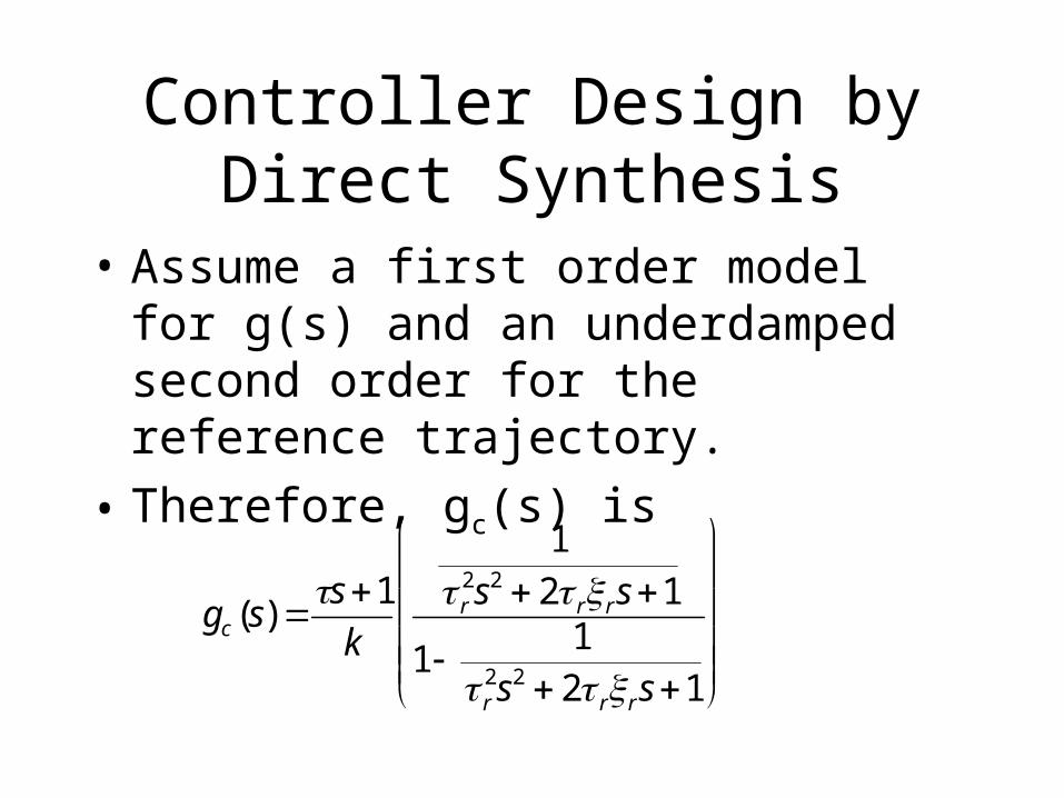
Controller Design by Direct Synthesis
• Assume a first order model for g(s) and an underdamped second order for the reference trajectory.
• Therefore, gc(s) is
gc (s) s1
k
1
r2s2 2 r rs1
1 1
r2s2 2 r rs1

Controller Design by Direct Synthesis
• After some algebra
gc (s) s1
k
1
r2s2 2 r rs

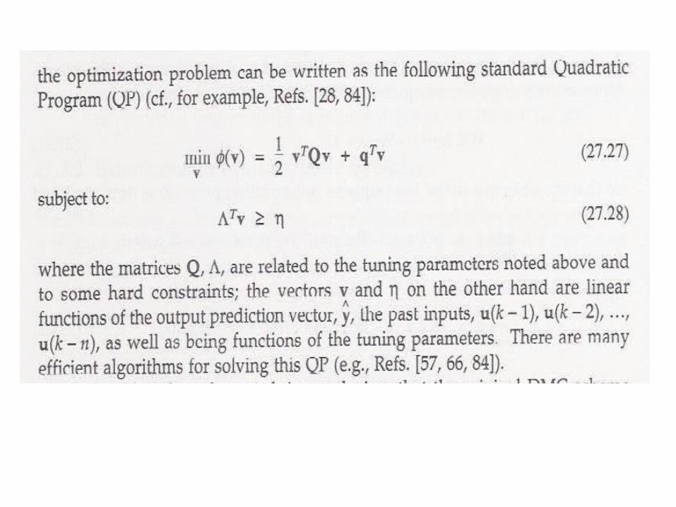
Model Predictive Control

MPC best suited for
• MIMO processes with significant interaction between SISO loops
• Either equal or unequal number of inputs
• Complex and usually problematic dynamics (longtime delays, and inverse response, or unusually large time constant)
• Constraints in inputs and/or outputs

Basic Elements of MPC
1. Trajectory
2. Output Prediction
3. Control Action Sequence
4. Error Prediction
Ogunaike

MPC Architecture
PredictionControl
Calculations
Set-point Calculations
Process
Model +-Model
Output
Residuals
Inputs
InputsPredicted
Output
Set points

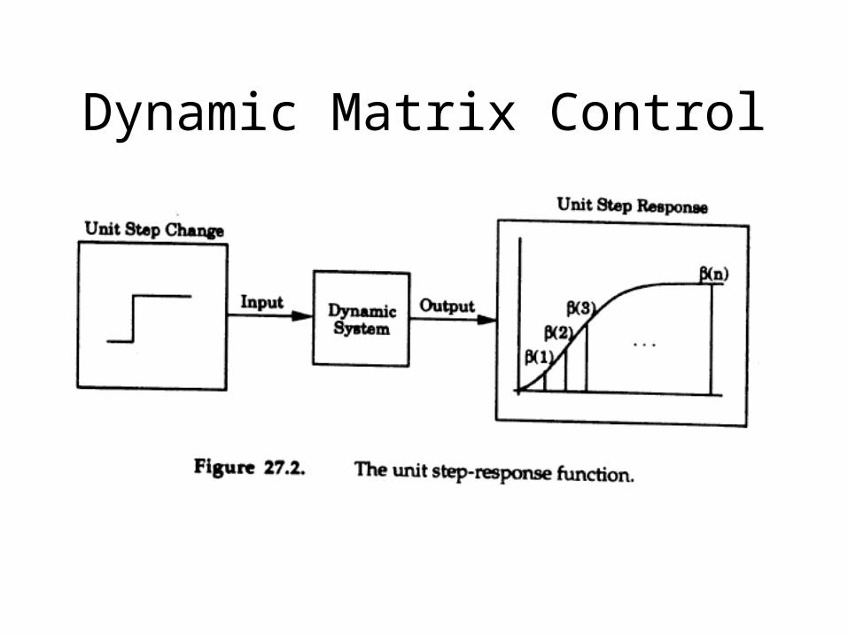
Prediction models• Finite convolution models
– Impulse-Response
– Step-Response
where
y(k) g(i)u(k i)i0
k
y(k) (i)u(k i)i0
k
g(i) (i) (1)
and (i) g( j)j1
i

Prediction models• Discrete State-Space
• Discrete Transfer function
where A(z-1) and B(z-1) are polynomials in z
y(k) a(i)y(k i)i0
k
b(i)u(k i m)i0
k
y(k) z mB(z 1)
A(z 1)u(z)
Dynamic Matrix Control
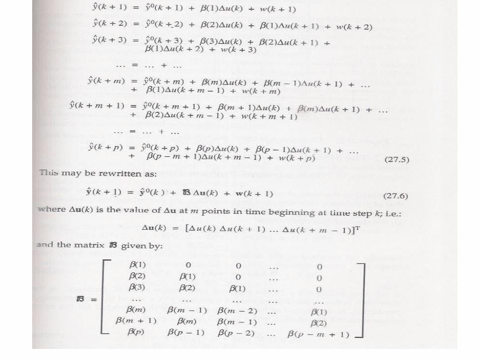


Unconstrained Problem Solution

Unconstrained Problem Solution

Unconstrained Problem solution

Unconstrained Problem solution

Unconstrained Problem solution
• In DMC, it is assumed that there exist disturbances unaccounted for by the model.
• It is further assumed that the best estimate of the values of these disturbances in the future of the elements– w(k+i), i=1,2, …, p of the vector w(k+1) is
estimated as


Model Algorithmic Control
• Similar to DMC with difference in the coefficients of the model and the reference trajectory– Process representation
– u is the actual input
– Output prediction
ˆ y (k 1) ˆ y 0(k)Gu(k) w(k 1)
ˆ y *(k 1) ˆ y 0(k)Gu(k) w(k 1)

Model Algorithmic Control
• In MAC, ŷ*(k+1) is defined typically as a reference trajectory based on the current measured value, y(k), and the current set point ysetpoint(k) as follows
with subsequent values determined according to
y*(k 1) y(k) (1 )ysetpoint(k); 0 < < 1
y*(k i) y(k i 1) (1 )ysetpoint (k); i > 1

Application of MPC to batchfluid bed drying

Modeling and Optimal Control of a FBDProcess Understanding: Drying theory
114
Drying CurveDrying Curve

Preliminaries Results
Dr. Velazquez, PhERL
4.5
5.5
6.5
7.5
8.5
9.5
10.5
1 2 3 4 5 6 7 8 9 10 11Sample number
% M
C
AF 40 T60
AF 50 T60
AF 60 T60
AF*60 T60
AF 70 T60
AF*80 T60
115
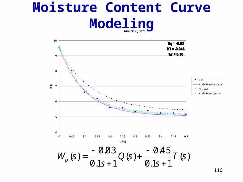
Moisture Content Curve Modeling
)(11.0
45.0)(
11.0
03.0)( sT
ssQ
ssWp
60m³/hr ; 60°C
4
5
6
7
8
9
10
0 0.05 0.1 0.15 0.2 0.25 0.3 0.35 0.4 0.45 0.5
t (hr)
Wp
Exp
Modelo en Laplace
AF1 Ave
Modelo en tiempo
116

In-Line NIR Measurements & Optimization
• Experimental design: 18 experimental combinations.
• Factors studied: bulk mass, air flow, and probe axial position.
• Response variable: residual (static – in-line NIR spectra).
• Region: drying equilibrium point (5 - 6 % H2O).
• Constant air’s inlet temperature = 70 °C
(same as in the calibration) 117

Axial Position Comparison
Analysis of Variance
118

Results
119

120
Results

121
Results

Rewriting of Transfer Function to fit MPC algorithm
• Can be transformed to describe the drying curve parting from any given point of the curve knowing the starting time and the current time of the process. Equation below describes the step wise function

Rewriting of Transfer Function to fit MPC algorithm
• The low order transfer equation proposed can be turned into the matrix form described by

Rewriting of Transfer
Function to fit MPC
algorithm

Closed loop of FBD
NIR
DCS-MPC
HXBlower
AirFlow
AirTemperature
MoistureMeasurement
125

FBD performance under MPC
126

FBD performance under MPC
127

128
FBD performance under MPC

Robustness test for error in modeling
Dr. Velazquez, PhERL 129

Comparison of performance for base and comparison cases

Comparison of performance for base and comparison cases
Conclusions of example• The drying curve can be described accurately with a
first order transfer function.
• The position of the sensor probe is critical for meaningful monitoring data.
• The MPC algorithm demonstrated to be capable of handling the model mismatch.
• The MPC application would minimize the energy consumption when compare to the open loop case. In the comparison case, the minimization decreased compare to the base case.