advanced simulation methods for the reliability analysis ...li/materials/lecture_ncepu.pdf ·...
TRANSCRIPT

Advanced Simulation Methods for the Reliability Analysis of Nuclear Passive Systems
Francesco Di Maio, Nicola Pedroni, Enrico Zio*
Politecnico di Milano, Department of Energy, Nuclear Division*Chaire SSDE-Foundation Europeenne pour l’Energie Nouvelle, EDF
Ecole Centrale Paris and Supelec
Contents
� Objective
� Reliability assessment of T-H passive systems
� Advanced Monte Carlo Simulation (MCS) methods
2
� Fast-running models: � Simplified T-H models� Bootstrapped Artificial Neural Networks (ANNs)
� Safety margins
� Conclusions

Objective 3
TO ADDRESS THE COMPUTATIONAL CHALLENGES RELATED TO THE MODELING AND RELIABILITY RELATED TO THE MODELING AND RELIABILITY
ASSESSMENT OF THERMAL-HYDRAULIC (T-H) PASSIVE SAFETY SYSTEMS

Contents
� Objective
� Reliability assessment of T-H passive systems
� Advanced Monte Carlo Simulation (MCS) methods
4
� Fast-running models: � Simplified T-H models� Bootstrapped Artificial Neural Networks (ANNs)
� Safety margins
� Conclusions

5Reliability assessment of Thermal-Hydraulic (T-H) passive safety systems
Advantages:
� Simplicity
“Passive”= no need of external input (energy source) to operate
“Thermal-Hydraulic” = use of moving working fluids (e.g., naturalcirculation-based decay heat removal)
� Simplicity
� Reduction of human interaction
� Reduction or avoidance of external electrical input of power/signals
Drawbacks:
� Lower economic competitiveness (with respect to active systems)
� UNCERTAINTY IN BEHAVIOR AND MODELING
RELIABILITY (FAILURE PROBABILITY) ASSESSMENT

6Uncertainties in T-H passive system behavior and modeling
Mechanical componentsWELL-KNOWN
W
T3 L3
Г
“Passive” components:the natural elements
(e.g., natural circulation)
Lackof data oroperating experience
Natural forces(gravity) comparable to counter-forces(friction)
BEHAVIOR MODELING
UNCERTAIN
SENSITIVE TO SURROUNDINGS(i.e., to small random variations)
UNCERTAIN PARAMETERS(e.g., heat transfer coefficients)
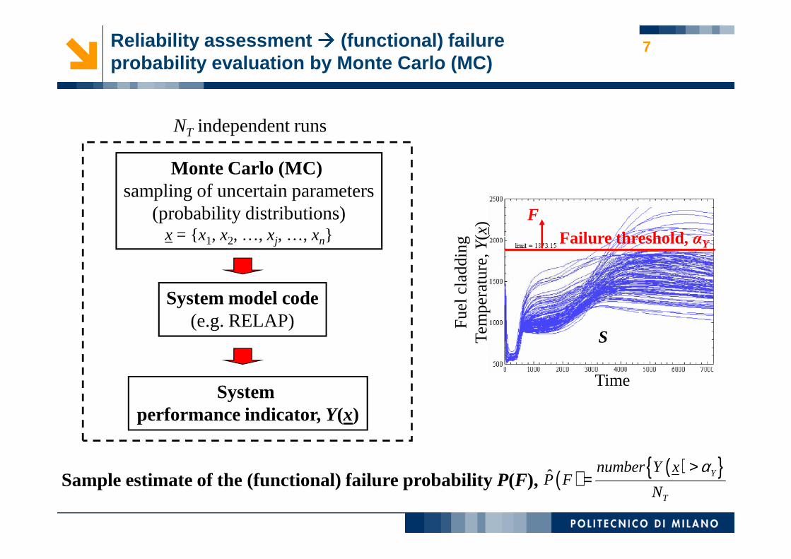
7Reliability assessment ���� (functional) failure probability evaluation by Monte Carlo (MC)
Monte Carlo (MC)sampling of uncertain parameters
(probability distributions)x = {x1, x2, …, xj, …, xn}
NT independent runs
Fue
l cla
ddin
gTe
mpe
ratu
re, Y(x
) FFailure threshold, αY
System model code(e.g. RELAP)
System performance indicator, Y(x)
Sample estimate of the (functional) failure probability P(F), ( ) ( ){ }ˆ Y
T
number Y xP F
N
α>=
Fue
l cla
ddin
gTe
mpe
ratu
re,
Time
S

8The Monte Carlo (MC)-based approach for (functional ) failure probability evaluation: drawbacks
( ) ( ){ }T
Y
N
xYnumberFP
α>=ˆ
SMALL NUMBER FORLONG CALCULATIONS!
SMALL NUMBER FORHIGHLY RELIABLE SYSTEMS!
S+
UNCERTAINTY/CONFIDENCE

9The Monte Carlo (MC)-based approach for (functional ) failure probability evaluation: contributions
ESTIMATION OF THE RELIABILITY (FUNCTIONAL FAILURE P ROBABILITY) OF T-H PASSIVE SYSTEMS
Long calculationsRare failure events Uncertainty/Confidence
1. Subset Simulation (SS)2. Line Sampling (LS)
Advanced MC Simulation methods
Fast-running models
2. Artificial Neural Networks(with bootstrap)
1. Simplified T-H models Order statistics(with bootstrap)
Safety margins
Contents
� Objective
� Reliability assessment of T-H passive systems
� Advanced Monte Carlo Simulation (MCS) methods
10
� Fast-running models: � Simplified T-H models� Bootstrapped Artificial Neural Networks (ANNs)
� Safety margins
� Conclusions

11The Monte Carlo (MC)-based approach for (functional ) failure probability evaluation: contributions
ESTIMATION OF THE RELIABILITY (FUNCTIONAL FAILURE P ROBABILITY) OF T-H PASSIVE SYSTEMS
Rare failure events
Advanced MC Simulation methods
1. Subset Simulation (SS)2. Line Sampling (LS)

121. Subset Simulation (SS)
x2Failure RegionF = F3
Target failure event, F
121 ... FFFFF mm ⊂⊂⊂⊂= −
Markov Chain Monte Carlo
Markov Chain Monte Carlo
(MCMC)
���� P(F3|F2)
m = 3
x1
F1
F2Standard
Monte Carlo Simulation(MCS)
Monte Carlo(MCMC)
���� P(F1)
���� P(F2|F1)
∏−
=+==
1
111 )|()()()(
m
iiim FFPFPFPFP

132. Line Sampling (LS)
x2 Failure Region, F
Key Idea: failure probability (P(F)) estimated using linespointing towards thefailure region F
j~P(F)(j)∑≈
NjFP
NFP )()(
1)(
x1
( )jx~ ~P(F)(j+2)
j+ 2~P(F)(j+1)
j+ 1 IF α ┴ FTHEN
VARIANCE ≈ 0
∑=
≈j
FPN
FP1
)()(
α
x⊥(α)
α = ‘important direction’

14Application: passive decay heat removal system of a Gas-cooled Fast Reactor (GFR)
Nine uncertain parameters, x (Gaussian):• Power• Pressure• Cooler wall temperature• Nusselt numbers (forced, mixed, free)• Friction factors (forced, mixed, free)• Friction factors (forced, mixed, free)
SYSTEM FUNCTIONAL FAILURE
Tout,core
( ){ }CxTx hotcoreout °>1200: ,
( ){ }CxTx avgcoreout °> 850: ,
F=
∩

15Application: results – (functional) failure probability estimation
( )FP̂( )FP̂
compt⋅=
2
1FOM
σ
Nloops= 3 (P(F) = 1.315·10-3)
FOM
Nloops= 4 (P(F) = 1.521·10-5)
FOM
Latin Hypercube Sampling (LHS) = benchmark simulation method in PRAStandard MCS
Comparison with:
( )FP̂( )FP̂ FOM
Standard MCS 1.600·10-3 216.00
SS 1.317·10-3 432.49
FOM
Standard MCS 0 2.31·104
SS 1.580·10-5 2.07·106
LHS 1.400·10-3 1.41·103
LS 1.314·10-3 1.00·106LHS 2.000·10-5 5.63·104
LS 1.510·10-5 9.87·108
E. Zio, N. Pedroni, “Estimation of the Functional Failure Probability of a Thermal-Hydraulic Passive System bySubset Simulation”,Nuclear Engineering and Design,2009, vol. 249(3), pp. 580-599.
E. Zio, N. Pedroni, “Reliability Analysis of Thermal-Hydraulic Passive Systems by Means of Line Sampling”,Reliability Engineering and System Safety, Vol. 9(11), 2009, pp. 1764-1781.
E. Zio, N. Pedroni, “How to effectively compute the reliability of a thermal-hydraulic passive system”,NuclearEngineering and Design, Volume 241, Issue 1, Jan. 2011, pp. 310-327.
NT = 1400 NT = 2300

16
1155 21450
0.5
1
1.5
2
2.5
3
3.5
4
4.5
x 10-3
Cond. level 0
1155 21450
0.5
1
1.5
2
2.5
3
3.5
4
4.5
x 10-3
Parameter x2 - Pressure [kPa]
Cond. level 1
1155 21450
0.5
1
1.5
2
2.5
3
3.5
4
4.5
x 10-3 Cond. level 2
1650 1650 1650
F1 F2 F3 = F
Unconditional PDFs
Conditional PDFs
1.4
1.6
1.8
2
Cond. level 0
1.4
1.6
1.8
2
Cond. level 1
1.4
1.6
1.8
2
Cond. level 2
Pressure, x2
, j = 1, …, 9, i = 1, 2, 3( )ijj Fxq |
( )jj xq , j = 1, …, 9
Application: results – (global) Sensitivity analysis by SS (1)
0.6 1.40
0.5
1
1.5
2
2.5
3
3.5
PD
F
Cond. level 0
0.6 1.40
0.5
1
1.5
2
2.5
3
3.5
Parameter x8 - Friction factor error (mixed convection)
Cond. level 1
0.6 1.40
0.5
1
1.5
2
2.5
3
3.5
Cond. level 2
1 1 1
Unconditional PDFs
Conditional PDFs≠
x2 and x8 are moreimportant than x3
in affecting system failure
72.00 108.000
0.2
0.4
0.6
0.8
1
1.2
1.4
PD
F
72.00 108.000
0.2
0.4
0.6
0.8
1
1.2
1.4
Parameter x3 - Cooler wall temperature [°C]72.00 108.000
0.2
0.4
0.6
0.8
1
1.2
1.4
90.00 90.00 90.00
Friction factormixed, x8
Cooler walltemperature, x3

17
0.1
0.2
0.3
0.4
0.5
0.6
0.7
0.8
0.9
( ) ( )( ) ( )FPxP
FxPxFP
j
jj
|| = , j = 1, …, 9
Global information:� whole range of variability of xj is considered
� all other parameters (xk, k ≠ j) vary as well
Bayes’ theorem:
P(F
| x 2
)
Pressure, x2
Application: results – (global) Sensitivity analysis by SS (2)
1250 1300 1350 1400 1450 1500 1550 1600 16500
0.6 0.7 0.8 0.9 1 1.1 1.2 1.30
0.01
0.02
0.03
0.04
0.05
0.06
0.07
0.08
70 75 80 85 90 95 100 1050
0.01
0.02
0.03
0.04
0.05
0.06
0.07
0.08
P(F
| x 3
)
P(F
| x 8
)
Friction factormixed, x8
Cooler walltemperature, x3

18
α tells which variables are more important in causing system failure
Application: results – (local) Sensitivity analysis by LS
LS important direction, α
Nloops α1 (x1) α2 (x2) α3 (x3) α4 (x4) α5 (x5) α6 (x6) α7 (x7) α8 (x8) α9 (x9)
4 + 0.0774 - 0.9753 + 0.0203 + 0.0032 - 0.1330 + 0.0008 + 0.0026 + 0.1534 - 0.0342
α tells which variables are more important in causing system failure
Agreement with SS and with reference case study of literaturePressure Nusselt mixed Friction mixed
E. Zio, N. Pedroni, “Monte Carlo Simulation-based Sensitivity Analysis of the model of a Thermal-Hydraulic PassiveSystem”, accepted for publication onReliability Engineering and System Safety, 2011.

19Line Sampling: technical issues
1. Determination of the “important direction” α���� additional runs of the T-H model code (↑ overall CPU cost)
Original contributions:� comparison of three literature methods for identifying α� use of Artificial Neural Networks (instead of the T-H code) to reduce
the computational cost associated to the identification of α
2. Efficiency of LS with small sample sizes (e.g., < 100)���� needed with T-H codes requiring hours for a single simulation (Fong et al., 2009)
the computational cost associated to the identification of α� proposal of a new method to determine α, based on the minimizationof
the varianceof the LS failure probability estimator
Original contribution:� challenging the performance of LS in the estimation of small failure
probabilities (~10-4) with a small number of samples drawn (i.e., << 100)

20LS – Technical issue 1: accurate determination of th e ‘important direction’ α – Original method proposed
Constrained minimization of the variance of the LS failure probability estimator

21LS – Technical issue 1: accurate determination of the ‘important direction’ α - Results
Practical case: low number of T-H code simulations
3.45
3.5
3.55
3.6
3.65x 10⁻⁴
Fa
ilure
pro
babi
lity,
P(F
)
Ncode= 100
Accuracy (proposed method) ~ (3 – 7)·Accuracy (literature methods)
3.15
3.2
3.25
3.3
3.35
3.4
Proposed method
Fa
ilure
pro
babi
lity,
MCMC Design point Gradient
Precision (proposed method) ~ (5 – 7)·Precision (literature methods)

22Line Sampling: technical issues
1. Determination of the “important direction” α���� additional runs of the T-H model code (↑ overall CPU cost)
Original contributions:� comparison of three literature methods for identifying α� use of Artificial Neural Networks (instead of the T-H code) to reduce
the computational cost associated to the identification of α
2. Efficiency of LS with small sample sizes (e.g., < 100)���� needed with T-H codes requiring hours for a single simulation (Fong et al., 2009)
the computational cost associated to the identification of α� proposal of a new method to determine α, based on the minimizationof
the varianceof the LS failure probability estimator
Original contribution:� challenging the performance of LS in the estimation of small failure
probabilities (~10-4) with a small number of samples drawn (i.e., << 100)

23LS – Technical issue 2: efficiency with small sample sizes - Results
Very smallsample size (ranging from 5 to 50)
1.2
1 .4
1 .6
1 .8
2x 10
-4
Fa
ilure
pro
babi
lity,
P(F
)
MAE = 5%
0 5 10 15 20 25 30 35 40 45 50 550.6
0 .8
1
Sample size, NT
Fa
ilure
pro
babi
lity,
MAE = 16%
MAE = 5%
MAE = 194%
95% CI = [0, 0.0582]Standard MCS with NT = 50
E. Zio, N. Pedroni, “An optimized Line Sampling method for the estimation of the failure probability of nuclear passivesystems”,Reliability Engineering and System Safety, Volume 95, Issue 12, Dec. 2010, pp. 1300-1313.

24Conclusions – Advanced MC Simulation methods: SS and LS
• SS and LS estimating the (functional) failure probability of T-H passive systems:
� Estimation of small failure probabilities (≤ 10-5)• Comparison with benchmark simulation methodsin PRA (standard MCS and LHS)
– SS and LS much more efficient than benchmark simulation methods in PRA
– LS performance almost independentof the failure probability � wide range of applications to real systems
• Optimization of the LS method → “important direction” based on minimization of the varianceof the LS failure probability estimator
– Combination of soft-computing methods (GA + ANN)
– More accurateand preciseestimates than other literature methods
• Successful LSwith very small sample sizes (5-50)
� Sensitivity analysis
• SS: “global” information based on a large amount of conditional samples
• LS: “local” information based on the “important direction ”

Contents
� Objective
� Reliability assessment of T-H passive systems
� Advanced Monte Carlo Simulation (MCS) methods
25
� Fast-running models: � Simplified T-H models� Bootstrapped Artificial Neural Networks (ANNs)
� Safety margins
� Conclusions

26The Monte Carlo (MC)-based approach for (functional ) failure probability evaluation: contributions
ESTIMATION OF THE RELIABILITY (FUNCTIONAL FAILURE P ROBABILITY) OF T-H PASSIVE SYSTEMS
Long calculations
Fast-running models
2. Artificial Neural Networks(with bootstrap)
1. Simplified T-H models

1. Simplified T-H models
Passive Residual Heat Removal System in theHigh Temperature Reactor Pebble Modular (HTR-PM)[in collaboration with Institute of Nuclear and New Energy Technology (INET)- Tsinghua University, Beijing, China]
Safety Parameter
27
Transparent and fast T-H MATLAB model(embedded within a Monte Carlo-driven fault injection engine to sample component failures)
F. Di Maio, E. Zio, L. Tao, J. Tong, “Passive System Accident Scenario Analysis by Simulation”, proceedings ofPSA2011, pp. 1718-1728,International Topical meeting on Probabilistic Safety Assessment and Analysis, March13-17, 2011, Wilmington, USA.

Application: passive Residual Heat Removal System i n the High Temperature Reactor Pebble Modular (HTR-PM)
N Parameter Distribution Note1 W Normal Residual heat power2 Ta,in Bi-Normal Temperature of inlet air in the air-cooled tower3 xi1 Uniform Resistance coefficient of elbow4 xi2 Uniform Resistance coefficient of header channel5 xiw Uniform Resistance coefficient of the water tank walls6
xia,in UniformSum of the resistance coefficients of inlet shutter and air coolingtower and silk net
7xia,out Uniform
Sum of the resistance coefficients of outlet shutter and air coolingtower and silk net
8 xia,narrow Uniform Resistance coefficient of the narrowest part of the tower9 Pa,in Uniform Pressure of the inlet air in the cooler tower10 dx Uniform Roughness of pipes11 Ha Normal Height of chimney12 La Normal Length of pipes in the exchanger13 Na Normal Total number of pipes in the air cooler14 Af Normal Air flow crossingarein thenarrowestpartof thetower
37 input parameters
14 Af Normal Air flow crossingarein thenarrowestpartof thetower15 Af,in Normal Inlet air flow crossing area in the tower16 Af,out Normal Outlet air flow crossing area from the tower17 Af,narrow Normal Crossing area in the narrowest part of the tower18 S1 Normal Distance between centers of adjacent pipes in horizontal direction19 S2 Normal Distance between centers of adjacent pipes in vertical direction20 S Normal Distance between fins in the ribbed pipe21 Da Normal Pipes inner diameter in the air cooling exchanger22 Do Normal Pipes outer diameter23 Douter Normal Rib outer diameter24 Pw Normal Water pressure in the pipes25 Hw Normal Elevatory height of water26 Nw Discrete Normal Number of water cooling pipes for each loop27 Lw Normal Length of the water cooling pipes28 Dw Normal Inner diameter of the water cooling pipes29 D1 Normal Inner diameter of the in-core and air cooler connecting pipes30 D2 Normal Inner diameter of the in-core header31 LC Normal Length of the in-core and air cooler connecting pipes (“cold leg”)32 LH Normal Length of the in-core and air cooler connecting pipes (“hot leg”)33 Ri Log-normal Thermal resistance of pipes inside of the heat exchanger34 Ro Log-normal Thermal resistance due to the dirt of the pipes fins35 Rg Log-normal Thermal resistance of the gap between fins36 Rf Log-normal Thermal resistance of fins37 lamd Normal Heat transfer coefficient of the pipes
1 output parameter: outlet water temperature
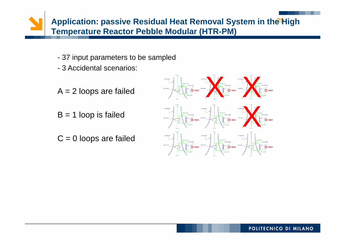
- 37 input parameters to be sampled- 3 Accidental scenarios:
A = 2 loops are failed
B = 1 loop is failed
X XX
29Application: passive Residual Heat Removal System i n the High Temperature Reactor Pebble Modular (HTR-PM)
C = 0 loops are failed
X

Acquire insights on the behavior of the system with respect to how much its output depends on the inputs
Model simplification by sensitivity analysis
Objective:
COMPUTATIONALLY BURDENSOMEDisadvantage:(several model computations)
comparison
30
VARIANCE DECOMPOSITION
SEVERAL MODEL
EVALUATIONS
Fast TH model of
RHR
ANALYTIC HIERARCHY PROCESS
SEVERAL MODEL
EVALUATIONSQualitative
resultsXY. Yu, T. Liu, J. Tong, J. Zhao, F. Di Maio, E. Zio, A. Zhang,“ Variance Decomposition Sensitivity Analysis of a Passive
Residual Heat Removal System Model” , Proceedings ofSAMO2010, Milano, July 2010, Procedia - Social andBehavioral Sciences, Volume 2, Issue 6, 2010, Pages 7772-7773.
Y. Yu, T. Liu, J. Tong, J. Zhao, F. Di Maio, E. Zio, A. Zhang, “Multi-Experts Analytic Hierarchy Process for the SensitivityAnalysis of Passive Safety Systems”,Proceedings of the 10th International Probabilistic Safety Assessment &Management Conference, PSAM10, Seattle, June 2010.
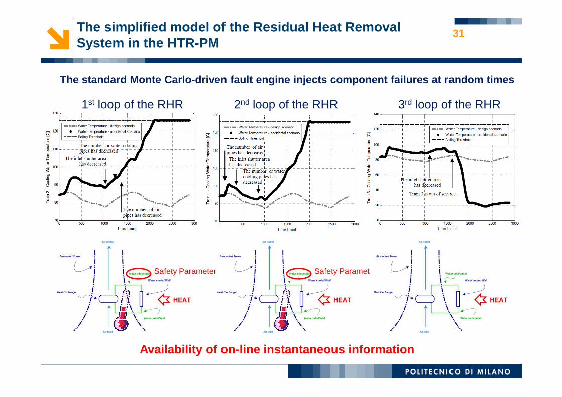
The simplified model of the Residual Heat Removal System in the HTR-PM
The standard Monte Carlo-driven fault engine inject s component failures at random times
1st loop of the RHR 2nd loop of the RHR 3rd loop of the RHR
31
Safety Parameter Safety Parameter
Availability of on-line instantaneous information

The Variance Decomposition Method
1 2( , )y m x x=Model
)]([)]([][ 11 2121XYVarEXYEVarYVar XXXX +=
][
)]([ 121
21
YVar
XYEVar XX=ηIndex of Importance of X1
][
)],([ 21,22,1
321
YVar
XXYEVar XXX=ηIndex of Importance of X1, X2(for a 3 inputs model X1,X2,X3)

Single parameter analysis: Index of importance 2Xη
3 accidental scenarios:
Index of Importance for single parameter contribution to the output variance

Group of parameters: index of Importance
3 accidental scenarios:
2η
Index of Importance for group parameter contribution to the output variance
The group sensitivity analysis allows underlining important physical and modelling aspects related to the system behaviour

The Analytic Hierarchy Process
Experts are asked to independently build the judgment matrix by:- defining the top goal of the hierarchy , e.g., capability of the RHR
system in removing the core decay power- defining the hierarchy structure , e.g.,
35
- comparing pairwise the model inputs with respect to their importance on the top goal, e.g.
- computing the priority vectors , i.e., importance of the inputs
Input 1 Input 2
Input 1 1 3
Input 2 1/3 1
1 = A and B equally important
3 = A slightly more important than B
5 = A strongly more important than B
7 = A very strongly more important than B
9 = A absolutely more important than B

Comparison between Variance Decomposition method and Analytic Hierarchy Process (AHP)
� Power W is importantthe same with AHP� Inlet air temperature Ta,in is
importantthe same with AHP� Water pressure Pw not identified as
important by AHP
N Parameter Variance Decomposition Analytic Hierarchy Process [*]1 W X X2 Ta,in X X3 xi1
4 xi2
5 xiw
6 xia,in
7 xia,out
8 xia,narrow
9 Pa,in
10 dx11 Ha
12 La
13 Na
14 Af
15 Af,in
16 Af,out
17 A
� All other parameters have minor impacts with respect to W and Ta,in
the same with AHP
AHP and Variance Decompositionprovide coherent results
17 Af,narrow
18 S1
19 S2
20 S21 Da
22 Do
23 Douter
24 Pw X25 Hw
26 Nw
27 Lw
28 Dw
29 D1
30 D2
31 LC
32 LH
33 Ri
34 Ro
35 Rg
36 Rf
37 lamd

372. Fast-running empirical regression models: Bootstrapped Artificial Neural Networks (ANNs)
�ANNs = empirical regression models
� generate a reducednumber (50-100) of I/O data examplesby running the T-H code
� train the ANN model to fit the data
� usethe ANN (instead of the T-H code) to calculate the output
�ANNs for practical use in passive system reliability assessment:
ANN REGRESSION MODEL → ADDITIONAL UNCERTAINTYANN REGRESSION MODEL → ADDITIONAL UNCERTAINTY
CONFIDENCE INTERVAL FOR THE QUANTITY OF INTEREST
BOOTSTRAP (ENSEMBLE) OF ANN REGRESSION MODELS
� each modelof the ensemble provides an estimateof the output
� the empirical distribution of the bootstrapped estimates is built
in our work:

38Application: passive decay heat removal system of a Gas-cooled Fast Reactor (GFR)
Nine uncertain parameters, x (Gaussian):• Power• Pressure• Cooler wall temperature• Nusselt numbers (forced, mixed, free)• Friction factors (forced, mixed, free)• Friction factors (forced, mixed, free)
SYSTEM FUNCTIONAL FAILURE
Tout,core
( ){ }CxTx hotcoreout °>1200: ,
( ){ }CxTx avgcoreout °> 850: ,
F=
∩

39Application – Bootstrapped ANNs: functional failure probability estimation
4
5
6
7
8
9
10x 10
-4 ANN-based BBC 95% CIs for P(F)
4
5
6
7
8
9
10x 10
-4 Quadratic RS-based BBC 95% CIs for P(F)
Comparison with quadratic Response Surfaces (RSs)(Arul et al., 2009; Fong et al., 2009; Mathews et al., 2009)
ANNs Quadratic RSs
Fai
lure
pro
bab
ility
, P(F
)
Fai
lure
pro
bab
ility
, P(F
)Reference result obtained by Monte Carlo Simulation with NT = 250000 samples!
(~ 417 h)
Total CPU time (ANN/RS) << 1/100·Total CPU time (T-H model)
10 20 30 40 50 60 70 80 90 100 110
0
1
2
3
4
10 20 30 40 50 60 70 80 90 100 110
0
1
2
3
4
Fai
lure
pro
bab
ility
,
Fai
lure
pro
bab
ility
,
Training sample size Training sample size
N. Pedroni, E. Zio, G. E. Apostolakis, “Comparison of bootstrapped Artificial Neural Networks and quadratic ResponseSurfaces for the estimation of the functional failure probability of a thermal-hydraulic passive system”,ReliabilityEngineering and System Safety, 95(4), 2010, pp. 386-395.

40Bootstrapped ANNs: first-order global Sobol sensitivity indices – Results
0.7
0.75
0.8
0.85
0.9
0.95
1
2
0.7
0.75
0.8
0.85
0.9
0.95
1
2
Pressure, x2Pressure, x2
So
bo
l in
dex
So
bo
l in
dex
ANNs Quadratic RSs
10 20 30 40 50 60 70 80 90 100 1100.6
0.65
p10 20 30 40 50 60 70 80 90 100 110
0.6
0.65
Reference result obtained by Monte Carlo Simulation with NT = 110000 samples!(~ 92 h)
�ANNs produces more accurate and precise estimates than quadratic RSs� CPU time (ANN) ~ 1.5·CPU time (RS)
Training sample size Training sample size
E. Zio, G. E. Apostolakis, N. Pedroni, “Quantitative functional failure analysis of a thermal-hydraulic passive system bymeans of bootstrapped Artificial Neural Networks”,Annals of Nuclear Energy, Volume 37, Issue 5, 2010, pp. 639-649.

41Conclusions - Fast-running models
• Simplified MATLAB T-H model:� dependenceof the system response on the time and magnitude of
components and equipments failures
� influenceof the uncertaintiesand of components and equipments failures on the system function
� accuracyand speed of calculation �required coverage of scenarios for safety
• ANNs for substituting the T-H code in the estimation of the functional • ANNs for substituting the T-H code in the estimation of the functional failure probability of T-H passive systems:� Estimation of small failure probabilities (~ 10-4)
• Small number (20-100) of T-H code runs to build the models → CPU cost ↓ by two orders of magnitude
• Bootstrap of ANN models → uncertainties (confidence intervals)of the estimates
• Estimation of first-order global Sobol sensitivity indices• Comparisonwith quadratic Response Surfaces
– better accuracies and precisions of ANNs
– slightly higher CPU cost associated to ANNs

Contents
� Objective
� Reliability assessment of T-H passive systems
� Advanced Monte Carlo Simulation (MCS) methods
42
� Fast-running models: � Simplified T-H models� Bootstrapped Artificial Neural Networks (ANNs)
� Safety margins
� Conclusions

43The Monte Carlo (MC)-based approach for (functional ) failure probability evaluation: contributions
ESTIMATION OF THE RELIABILITY (FUNCTIONAL FAILURE P ROBABILITY) OF T-H PASSIVE SYSTEMS
Uncertainty/Confidence
Order statistics(with bootstrap)
Safety margins

Safety margin quantification
( )2200MAXcladT F≤ °
( )cladT
Confidence Interval
Confidence Interval
Confidence Interval
44
Uncertainty in safety margins calculation by numerical code• Input values
• Modeling hypotheses
Interval
E. Zio, and F. Di Maio, “Bootstrap and Order Statistics for Quantifying Thermal-Hydraulic Code Uncertainties in theEstimation of Safety Margins”,Science and Technology of Nuclear Installations, Volume 2008, Article ID 340164, 9pages, doi:10.1155/2008/340164

- 37 input parameters to be sampled- 3 Accidental scenarios:
A = 2 loops are failed
B = 1 loop is failed
X XX
AIM: estimates of the 95th percentiles of the safety parameters distributions
45Application: passive Residual Heat Removal System i n the High Temperature Reactor Pebble Modular (HTR-PM)
� Bootstrapped Order Statistics (BOS)Minimum Minimum numbernumber ofof simulationssimulations N N forfor estimatingestimating the the distributiondistribution ofof the the safetysafety parameterparameter withwith a a givengiven confidenceconfidence, , accounting accounting alsoalso forfor the the uncertaintyuncertainty ofof the the empiricalempirical modelmodel usedused toto simulate the simulate the accidentalaccidental scenariosscenarios
COMPUTATIONAL BURDEN
C = 0 loops are failed
X

Results: Two RHR loops are enoughThe 3rd loop can be considered as a redundancy
Number of simulations N for each accidental scenario: 50Number of Bootstrap replications : 100
46Application: passive Residual Heat Removal System i n the High Temperature Reactor Pebble Modular (HTR-PM)
E. Zio, F. Di Maio, J. Tong, “Safety Margins Confidence Estimation for a Passive Residual Heat Removal System”,Reliability Engineering and System Safety,Vol. 95, 2010, pp. 828–836

results in:Similarity of the 95th percentile point- estimates (reliability)
Narrowing the confidence intervals (robustness)
Approaching down the estimates to the true value (conservativeness)
… increasing the number of simulations
47Application: passive Residual Heat Removal System i n the High Temperature Reactor Pebble Modular (HTR-PM)
Contents
� Objective
� Reliability assessment of T-H passive systems
� Advanced Monte Carlo Simulation (MCS) methods
48
� Fast-running models: � Simplified T-H models� Bootstrapped Artificial Neural Networks (ANNs)
� Safety margins
� Conclusions

Conclusions
• Objective:
• Contributions:
� Advanced Monte Carlo Simulation methods:
� SSand LS for the reliability analysis of a T-H passive system
� Optimization of the LS method (variance-minimizing search of “important direction” α)
49
To address the computational challenges related to the reliability analysis of Thermal-Hydraulic (T-H) passive safety systems
� Successful LS performancewith very small sample sizes
� Fast-running models:
� MATLAB implementation of a simplified T-H model
� ANNs for the reliability analysis of a T-H passive system
� ANN regression model uncertainty quantification by bootstrap
� Safety margins
� Percentileestimation by order statistics
� Percentile uncertainty quantification by bootstrap