advanced statistical methods for observational studies

L E C T U R E 0 4

Advanced Statistical Methods for Observational Studies

class management

Projects

Come talk to us.

The idea is you will do a 10 minute presentation (slide deck) for the two of us and we’ll ask you questions. (Last year we held these in David’s office.)

Take home exam will go up on the website this Friday.

Will be due 10 days later (Monday class time).

Physical copies (not electronic).

Questions?

unobserved confounding

There are more things in heaven and earth, Horatio,Than are dreamt of in your philosophy.-Hamlet (1.5.167-8)

Design of Observational Studies: chapter 3.4-3.8

naïve model

Model

Assumptions

Implementation

naïve model: “natural” experiments

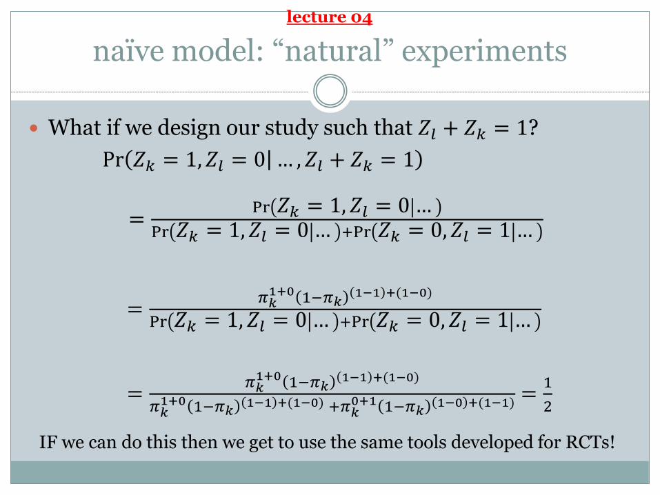
What if we design our study such that 𝑍𝑙 + 𝑍𝑘 = 1?

Pr 𝑍𝑘 = 1, 𝑍𝑙 = 0 … , 𝑍𝑙 + 𝑍𝑘 = 1

=Pr 𝑍𝑘 = 1, 𝑍𝑙 = 0 …

Pr 𝑍𝑘 = 1, 𝑍𝑙 = 0 … +Pr 𝑍𝑘 = 0, 𝑍𝑙 = 1 …

=𝜋𝑘1+0 1−𝜋𝑘

1−1 +(1−0)

Pr 𝑍𝑘 = 1, 𝑍𝑙 = 0 … +Pr 𝑍𝑘 = 0, 𝑍𝑙 = 1 …

=𝜋𝑘1+0 1−𝜋𝑘

1−1 +(1−0)

𝜋𝑘1+0 1−𝜋𝑘

1−1 +(1−0) +𝜋𝑘0+1 1−𝜋𝑘

1−0 +(1−1) =1

2

IF we can do this then we get to use the same tools developed for RCTs!

lecture 04

naïve model: assumption one

Strongly Ignorable Treatment Assignment: Those that look alike (in our data set) are alike

𝜋𝑖 = Pr 𝑍𝑖 = 1 𝑟𝑇𝑖 , 𝑟𝐶𝑖 , 𝒙𝑖 , 𝑢𝑖 = Pr 𝑍𝑖 = 1 𝒙𝑖and

0 < 𝜋𝑖 < 1 for all i = 1, 2, …, n

If two subjects have the same propensity score, then their values of xmay be different.

By SITA, if these two subjects have the same e(x) then the differences in their x are not predictive of treatment assignment (i.e., 𝒙 ⊥ 𝑍|𝑒(𝒙)).

Therefore the mismatches in x will be due to chance and will tend to balance. (more details)

∥

lecture 04

http://biomet.oxfordjournals.org/content/70/1/41.full.pdf+html

naïve model: assumption two

No Interference Between Units (part of SUTVA): the observation on one unit should be unaffected by particular assignment of treatments to other units.

Can be written as:𝑅𝑖(𝑍𝑖 = 𝑧𝑖) = 𝑅𝑖(𝒁

∗)

where 𝑍𝑖 = 𝑧𝑖 indicates the treatment level for the ith unit and 𝒁∗ is a particular randomization from the set of all randomizations that have 𝑍𝑖 = 𝑧𝑖.

Not true for most educational interventions and infectious disease applications.

More details here and here.

http://www.biostat.jhsph.edu/~dscharf/Causal/rubin.journ.psych.ed.pdf

http://www-stat.wharton.upenn.edu/~rosenbap/interference.pdf

naïve model: implementation

Collect a bunch of covariates that are related to treatment level and to the outcome.

Exact match if you can.

You probably can’t exact match so estimate propensity scores and match on a hybrid of pscores and Mahalanobisdistance.

Play around with the matching until you achieve acceptable comparison groups.

Die a little bit inside when you read your critics’ reviews because they point out all of the confounding that could exist. Reevaluate life choices.

sensitivity analysis

Sensitivity models are a means for moving past the “you didn’t do X which could lead to bias” argument.

A useful sensitivity model addresses one assumption at a time, quantifying and making understandable the impact of departures from the assumption being assessed.

We’re going to discuss the Γ sensitivity model which addresses the ignorable treatment assignment (SITA), not interference (SUTVA).

sensitivity analysis

A word of warning: many people find the Γ sensitivity model confusing. This lecture will only give you a sense of what’s going on with this model;

it isn’t intended to be sufficient to fully understand Γ sensitivity.

Read section 3.4-3.8.

If you are so inclined then this might be a very nice place to produce your own framework for sensitivity.

model: sensitivity analysis

Start with two observational units who have probability of treatment 𝜋𝑖 and 𝜋𝑗 (which may not be the same values).

Recall we defined this as 𝜋𝑖 = Pr 𝑍𝑖 = 1 𝑟𝑇𝑖 , 𝑟𝐶𝑖 , 𝒙𝑖 , 𝑢𝑖 .

We can talk about the odds of i receiving treatment:𝜋𝑖

1 − 𝜋𝑖

And we can put the odds into a ratio:𝜋𝑖/(1 − 𝜋𝑖)

𝜋𝑗/(1 − 𝜋𝑗)


Our sensitivity model asserts that we can bound the odds ratio like so:

1

Γ≤𝜋𝑖/(1 − 𝜋𝑖)

𝜋𝑗/(1 − 𝜋𝑗)≤ Γ

whenever 𝒙𝑖 = 𝒙𝑗.

We are making a particular statement about how “far off” the actual treatment probabilities are from the pscore(which only depends on the observed covariates).

If Γ = 1 then this forces 𝜋𝑖 = 𝜋𝑗.

If Γ = 2 then 𝜋𝑖 can depart from 𝜋𝑗 For example: if 𝜋𝑖 = 1/2 and 𝜋𝑗 = 2/3 then

𝜋𝑖/(1 − 𝜋𝑖)

𝜋𝑗/(1 − 𝜋𝑗)=

0.5/(1 − 0.5)

0. 6 /(1 − 0. 6)= 2


With this model in place we can think about “worst case” scenarios regarding violations of SITA.

If someone is willing to give you a particular framework for how the violation must occur (to the exclusion of all other possible ways it can fail) then use that parametric model.

The Γ sensitivity model is non-parametric and we look at the extreme values that might occur when Γ > 1. We’ll get ranges of p-values and estimates

Every study is sensitive to sufficiently large violations of the SITA assumption. Just let Γ → ∞.

If we’re going to make progress then the question becomes what level of Γ is sufficiently large to proceed.

naïve model: “natural” experiments

What if we design our study such that 𝑍𝑙 + 𝑍𝑘 = 1?

Pr 𝑍𝑘 = 1, 𝑍𝑙 = 0 … , 𝑍𝑙 + 𝑍𝑘 = 1

=Pr 𝑍𝑘 = 1, 𝑍𝑙 = 0 …

Pr 𝑍𝑘 = 1, 𝑍𝑙 = 0 … +Pr 𝑍𝑘 = 0, 𝑍𝑙 = 1 …

=𝜋𝑘1+0 1−𝜋𝑘

1−1 +(1−0)

Pr 𝑍𝑘 = 1, 𝑍𝑙 = 0 … +Pr 𝑍𝑘 = 0, 𝑍𝑙 = 1 …

=𝜋𝑘1+0 1−𝜋𝑘

1−1 +(1−0)

𝜋𝑘1+0 1−𝜋𝑘

1−1 +(1−0) +𝜋𝑘0+1 1−𝜋𝑘

1−0 +(1−1) =1

2

IF we can do this then we get to use the same tools developed for RCTs!

lecture 04


If we design our study such that 𝑍𝑙 + 𝑍𝑘 = 1:

Pr 𝑍𝑘 = 1, 𝑍𝑙 = 0 … , 𝑍𝑙 + 𝑍𝑘 = 1 =𝜋𝑖

𝜋𝑖+𝜋𝑗

Combining this with the sensitivity model, and doing some vaguely enjoyable algebra, we get:

1

1 + Γ≤

𝜋𝑖𝜋𝑖 + 𝜋𝑗

≤Γ

1 + Γ

We get ½ if Γ = 1.


The randomization tests we have can be reworked under the understanding that we can vary the odds ratio within

1

1 + Γ≤


≤Γ

1 + Γ

Setting 𝜋𝑖

𝜋𝑖+𝜋𝑗=

Γ

1+Γwill get you one extreme.

Setting1

1+Γ=

𝜋𝑖

𝜋𝑖+𝜋𝑗will get you the other.

For notational purposes, let’s say that the usual Wilcoxon signed rank test (when Γ = 1) is written as 𝑇.

( S E E L E C T U R E 0 4 F O R M O R E D E T A I L )

Wilcoxon rank-sign test

the Wilcoxon signed rank

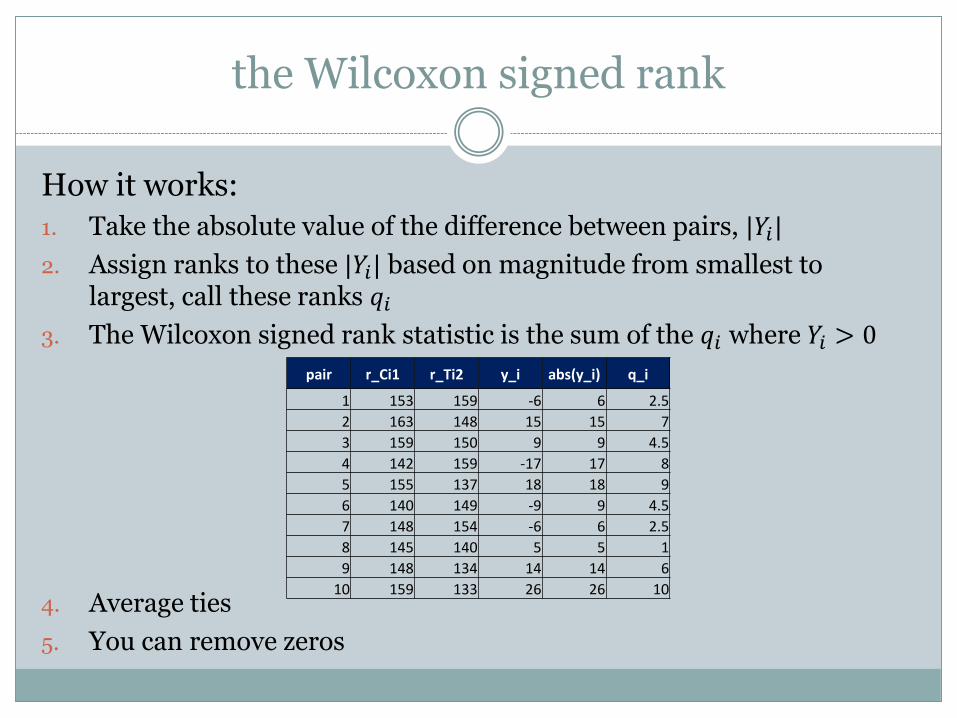
How it works:

1. Take the absolute value of the difference between pairs, |𝑌𝑖|

2. Assign ranks to these |𝑌𝑖| based on magnitude from smallest to largest, call these ranks 𝑞𝑖

3. The Wilcoxon signed rank statistic is the sum of the 𝑞𝑖 where 𝑌𝑖 > 0

4. Average ties

5. You can remove zeros

pair r_Ci1 r_Ti2 y_i abs(y_i) q_i

1 153 159 -6 6 2.5

2 163 148 15 15 7

3 159 150 9 9 4.5

4 142 159 -17 17 8

5 155 137 18 18 9

6 140 149 -9 9 4.5

7 148 154 -6 6 2.5

8 145 140 5 5 1

9 148 134 14 14 6

10 159 133 26 26 10


The randomization tests we have can be reworked under the understanding that we can vary the odds ratio within

1

1 + Γ≤


≤Γ

1 + Γ

Setting 𝜋𝑖

𝜋𝑖+𝜋𝑗=

Γ

1+Γwill get you one extreme.

Setting1

1+Γ=

𝜋𝑖

𝜋𝑖+𝜋𝑗will get you the other.

For notational purposes, let’s say that the usual Wilcoxon signed rank test (when Γ = 1) is written as 𝑇.

Then we’ll write the test statistic under our sensitivity model as 𝑇.

( E N D I N T E R L U D E )

Sensitivity analysis


We can calculate the exact distribution of 𝑇 under either extreme, but for large matched sets it’ll be easier (and not far off) to use an approximation.

The 𝑇 has known expected value and variance

𝐸 𝑇 =Γ

1 + Γ

I(I + 1)

2

𝑣𝑎𝑟( 𝑇) =Γ

1 + Γ 2

I(I + 1)(2I + 1)

6

where I is the number of matched pairs.


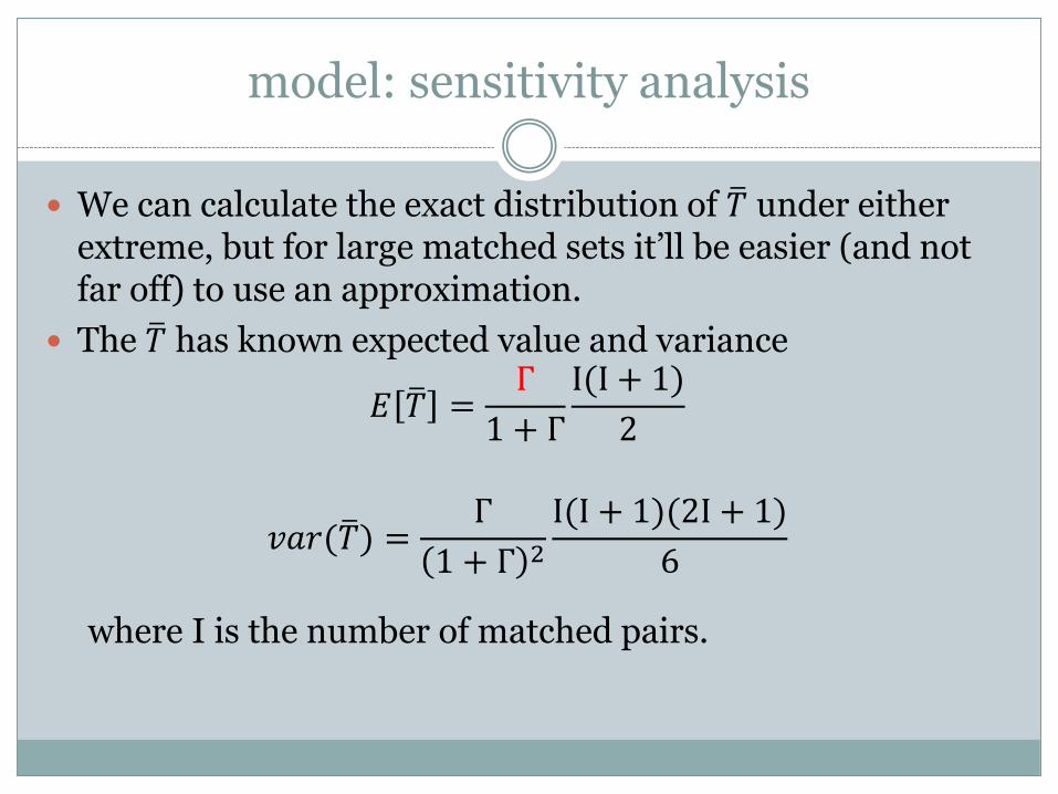
We can calculate the exact distribution of 𝑇 under either extreme, but for large matched sets it’ll be easier (and not far off) to use an approximation.

The 𝑇 has known expected value and variance

𝐸 𝑇 =1

1 + Γ

I(I + 1)

2

𝑣𝑎𝑟( 𝑇) =Γ

1 + Γ 2

I(I + 1)(2I + 1)

6

where I is the number of matched pairs.


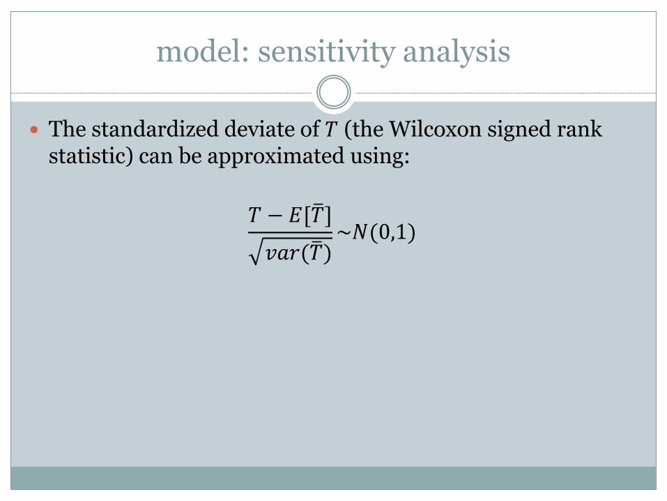
The standardized deviate of 𝑇 (the Wilcoxon signed rank statistic) can be approximated using:

𝑇 − 𝐸[ 𝑇]

𝑣𝑎𝑟( 𝑇)~𝑁(0,1)

example: sensitivity analysis

Similar to data set from lecture 03, but different number of observations and outcome of interest.

obs b_weight gest_age dose hearing

1 2412 36 1 0.12

2 2205 29 1 0.24

3 2569 36 1 0.02

4 2443 34 1 -0.16

5 2569 36 0 0.58

6 2436 35 0 -0.22

7 2461 34 0 -0.07

8 2759 32 0 -0.55

9 2324 27 0 -0.36

10 2667 34 0 0.28… … … … …

500 2349 33 1 -0.55


Outcome of interest: Hearing is some standardized metric with population mean=0 and sd=1.

obs b_weight gest_age dose hearing

1 2412 36 1 0.12

2 2205 29 1 0.24

3 2569 36 1 0.02

4 2443 34 1 -0.16

5 2569 36 0 0.58

6 2436 35 0 -0.22

7 2461 34 0 -0.07

8 2759 32 0 -0.55

9 2324 27 0 -0.36

10 2667 34 0 0.28… … … … …

500 2349 33 1 -0.55


Create 250 pair matches.

Using 𝑇, the usual Wilcoxon signed rank statistic:

We know that E[ 𝑇]=14,835 and sd( 𝑇)=810

Get T=13,250

Using the approximation:

𝑇 − 𝐸[ 𝑇]

𝑣𝑎𝑟( 𝑇)~𝑁(0,1)

13,250−14,835

810= −1.95, which has a p-value close to 0.05.

Interpretation: If there was a small amount of bias Γ = 1.12then this would nullify our qualitative claims.

𝐸 𝑇 =1

1 + Γ

I(I + 1)

2

Set Γ=1.11

implementation: sensitivity analysis

In practice, software will do this for you and you will interpret.

The key to keep in mind is that there are two different way things could go wrong: (i) units could be sorted into treatment or (ii) into control.

This gives rise to three different distributions:

Naïve model: T~N(I I+1

4,I(I+1)(2I+1)

24)

Biased toward one way: T~N(Γ

1+Γ

I I+1

2,

Γ

1+Γ 2

I(I+1)(2I+1)

6)

Biased other way: T~N(1

1+Γ

I I+1

2,

Γ

1+Γ 2

I(I+1)(2I+1)

6)


Use the new distributions to test your statistic to see where its critical values are.

This will lead you to provide wider intervals for everything: If you had a point estimate of (to pick a random number): 5 then, for a

particular Γ, you may end up with a “point estimate” of (4, 6). This new interval is not due to randomness in assignment, it is due to the difference in treatment assignment probabilities.

If you had a p-value of 0.012 , for a particular Γ, you may end up with a p-value interval of (0.032, 0.0001).


In practice, it’s common to just report the value of Γ which nullifies your qualitative conclusions (i.e., goes from significant to insignificant), and to help the reader in interpreting the meaning of Γ.

For example, Γ = 2 means that within a given pair – even though the two matched individuals looked identical in the data set – the actual odds of assignment was up to twice as likely for one member in the pair than the other. Likely this difference is due to the unobserved covariates.

The question then becomes: Is what’s left lingering out there, outside of your data set, enough to cause that level of confounding?

sensitivity analysis: understanding gamma

When you report Gamma, you report the maximal Gamma that still returns a qualitatively similar conclusion (e.g., if you found the treatment positive and significant then you report the value of Gamma that just barely makes the test not-significant).

Note: This says nothing about the case at hand. You are looking at the strength of the argument (i.e., how many in treated need to be switched to control before null). But we haven’t measured the level of unobserved (it’s still unobserved!!).

This is like saying a building can withstand a magnitude 8 earthquake. There is no statement in there about what magnitude earthquake the building will experience.

sensitivity analysis: understanding gamma

Explaining Gamma sensitivity is hard because the concept of confounding is tough.

Confounding (usually) arises from sorting into treatment/control (propensity - Fisher) on variables important in determining the outcome (prognostic – Mill).

Gamma sensitivity is kind of weird because it only focusses on the propensity, and then assumes the worst case for prognostic.

an example

Design of Observational Studies: chapter 5ish

matching on more than one metric

Intuition: matching on just propensity scores is like uniform randomization, whereas a Mahalanobis & pscoresis more like a matched pairs randomization.

example

Example: House examines the patient and wants to treat for sarcoidosis. He is always considering treating for sarcoidosis… but in a way that is unrelated to how sick the patient is.

To make this example easier to follow, let’s consider two data generating functions 1. Treatment:

2. Outcome:

0 1

0 0.5 0.1

1 0.5 0.1A

B

0 1

0 0.1 0.1

1 0.5 0.5A

B

propensity score vs. prognostic score

This departure arises when the variables predictive of treatment differs from the prognostically relevant variables

This insight led to an interesting paper: Bhattacharya & Vogt “Do Instrumental Variables Belong in Propensity Scores?”

Prognostic score is one way to address this: Ben Hansen “The prognostic analog of the propensity score”

http://www.nber.org/papers/t0343

http://biomet.oxfordjournals.org/content/95/2/481.short

The Buffalo

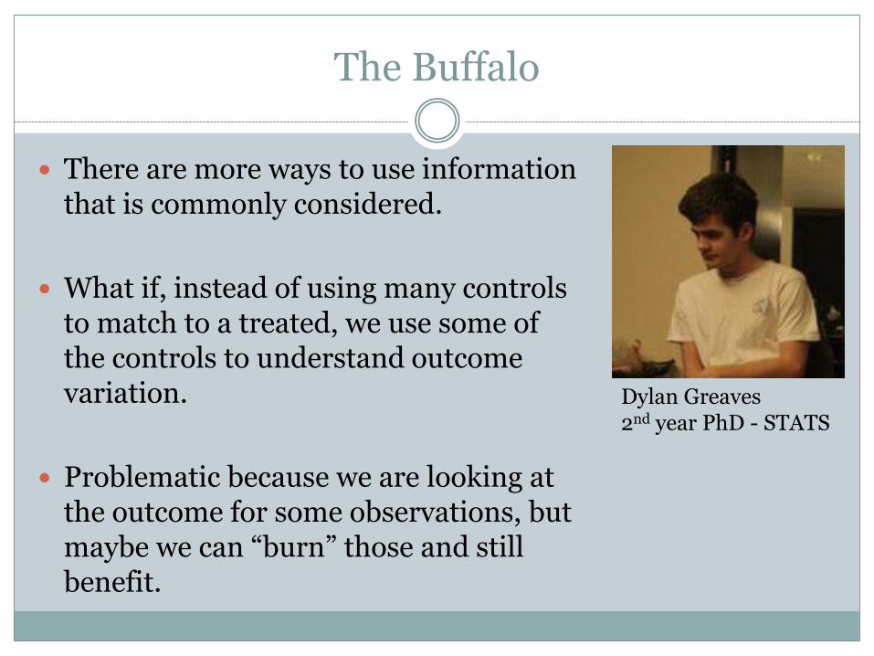
Dylan Greaves2nd year PhD - STATS

There are more ways to use information that is commonly considered.

What if, instead of using many controls to match to a treated, we use some of the controls to understand outcome variation.

Problematic because we are looking at the outcome for some observations, but maybe we can “burn” those and still benefit.

T Y

C

treatment effectp

rop

ensi

ty

treated

control

The Buffalo

takeaway

This toy example highlights that the propensity score focuses on treatment, which may be unrelated to outcomes.

This is OK – the theory of inference is predicated on randomization, not identical units going into the groups (Fisher)

But it is better to start with similar groups (Mill)

a second outcome

Design of Observational Studies: chapter 5.2.3 and 5.2.4Rosenbaum, “The Role of Known Effects in Observational Studies”

http://www.jstor.org/stable/2531497?seq=1#fndtn-page_scan_tab_contents

the structure of the argument: two outcomes

If your theory is well developed then you might be able to locate multiple outcomes that will support your understanding of the mechanism of the intervention.*

Two ways this can happen: The second outcome can be compatible (show violation)

The confirmation of a “null effect” can help rebuff claims of unobserved biases

*Keep this idea separate from “intermediate effects,” not because there’s a deep fundamental difference in these concepts but rather conflating them will tend to confuse discussions.

coherence

(Rough) Definition: A claim is made that an intervention must have a certain form (i.e., there’s a detailed hypothesis). In this situation, coherence means a pattern of observed associations compatible with this anticipated form, and incoherence means a pattern of observed associations incompatible with this form.

Claims of coherence or incoherence are arguable to the extent that the anticipated form of treatment effect is arguable.

If you want to see the technical details of how to build a statistical argument around this then check out Observational Studies, section 17.2 (coherent signed rank statistic).

Y2

X1

X2

X3

Xp

…

P1

P2

P4

P3

coherence

Y1

Y3

= rape

= unplanned

pregnancy

= STI

Y4 = test scores

I

the structure of the argument: null effect outcomes

Basic idea: Suppose that a treatment is known to not change a particular outcome. Then if we see differences between the treatment and control groups on this particular outcome, this must mean that there are differences between the treatment and control group on unmeasured covariates and thus there is hidden bias.

example: methylmercury fish

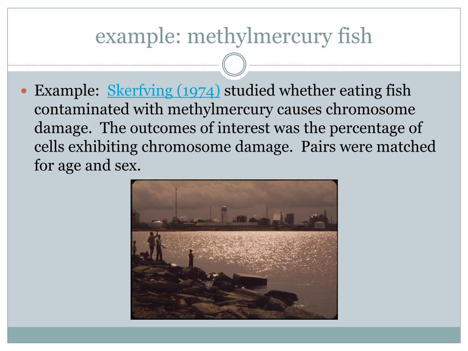
Example: Skerfving (1974) studied whether eating fish contaminated with methylmercury causes chromosome damage. The outcomes of interest was the percentage of cells exhibiting chromosome damage. Pairs were matched for age and sex.

http://www.ncbi.nlm.nih.gov/pubmed/4856767


Example: Skerfving (1974) studied whether eating fish contaminated with methylmercury causes chromosome damage. The outcomes of interest was the percentage of cells exhibiting chromosome damage. Pairs were matched for age and sex.

control.cu.cells <- c(2.7,.5,0,0,5,0,0,1.3,0,1.8,0,0,1,1.8,0,3.1)

exposed.cu.cells <- c(.7,1.7,0,4.6,0,9.5,5,2,2,2,1,3,2,3.5,0,4);

library(exactRankTests)

wilcox.exact(exposed.cu.cells,control.cu.cells,paired=TRUE)

Exact Wilcoxon signed rank test

data: exposed.cu.cells and control.cu.cells

V = 84, p-value = 0.04712

alternative hypothesis: true mu is not equal to 0

http://www.ncbi.nlm.nih.gov/pubmed/4856767


In the absence of hidden bias, there’s evidence that eating large quantities of fish containing methylmercury causes chromosome damage.

Going further, Skerfving described other health conditions of these subjects including other diseases such as (i) hypertension, (ii) asthma, (iii) drugs taken regularly, (iv) diagnostic X-rays over the previous three years, (v) and viral diseases such as influenza.

These can be considered outcomes since they describe the period when the exposed subjects were consuming contaminated fish.

However, it is difficult to imagine that eating fish contaminated with methylmercury causes influenza or asthma, or prompts X-rays of the hip or lumbar spine.


The data control.other.health.conditions <- c(rep(0,8),2,rep(0,3),2,1,4,1)

exposed.other.health.conditions <- c(0,0,2,0,2,0,0,1,1,2,0,9,0,0,1,0)

> wilcox.exact(control.other.health.conditions,exposed.other.health.conditions)

Exact Wilcoxon rank sum test

data: control.other.health.conditions and exposed.other.health.conditions

W = 112.5, p-value = 0.5257

alternative hypothesis: true mu is not equal to 0

There is no evidence of hidden bias.

But absence of evidence is not evidence of absence.


Questions: (1) When does such a test have a reasonable prospect of detecting hidden bias?

(2) If no evidence of hidden bias is found, does this imply reduced sensitivity to bias in the comparisons involving the outcomes of primary interest?

(3) If evidence of bias is found, what can be said about its magnitude and its impact on the primary comparisons?

null effect outcomes

Power of the test of hidden bias: Let y denote the outcome for which there is a known effect of zero. For a particular unobserved covariate u, what unaffected outcome y would be useful in detecting hidden bias from u?

Precise statement of results in: “The Role of Known Effects in Observational Studies”

Basic result: The power of the test of whether y is affected by the treatment increases with the strength of the relationship between y and u. If one is concerned about a particular unobserved covariate u, one should search for an unaffected outcome y that is strongly related to u.

http://www.jstor.org/stable/2531497?seq=1#fndtn-page_scan_tab_contents

takeaway

Having a detailed understanding of how your intervention functions, what the causal pathway includes and excludes, will give you more data sources that may validate or refute your hypothesis.

Coherence is trying to flesh out your hypothesis.

Known null effects may help to address unobserved confounding

T W O P R O B L E M S T W O C O N T R O L S

a second control group

Design of Observational Studies: chapter 5.2.2Rosenbaum, “The Role of a Second Control Group in an Observational Study”

http://projecteuclid.org/euclid.ss/1177013232

structure of argument

In an RCT the control and treatment groups are created from a pool of study participants. The assignment to C or T is due to a researcher-directed mechanism (e.g., flipping a coin, or matched pairs). Importantly: all participants can receive C or T.

In an observational study there are possibly many different reasons for people to have not received the treatment.

In some situations there are discernable subgroups within the non-treatment group, each subgroup being identifiable by the reason for the subgroup not receiving the treatment.

In some subset of these situations these subgroups will be open to critiques of bias when compared to the treatment group, but at least two of the subgroups will differ in the nature of their bias.

The contrast of these two control groups with the treatment group may strengthen your analysis.

second control group: army toxicity

Example: The army is interested in the long term effects of exposure to a list of specific chemical agents that were suspected of being toxic. Relatively few soldiers were exposed to these chemicals.


Example: The army is interested in the long term effects of exposure to a list of specific chemical agents that were suspected of being toxic. Relatively few soldiers were exposed to these chemicals.

At first pass, one might think to compare these exposed (“treated”) service members to service members who were not exposed at all.

Complicating that comparison, though, is that the army sorted people into jobs which exposed them or to jobs which did not.

The army used medical examinations – which were not well documented – to sort some individuals out of high-exposure jobs. This leaves the comparison between exposed and strictly unexposed potentially biased due to baseline conditions.


A second control group was constructed using service members who were in jobs which exposed them to chemical agents, but not the specific list of chemical agents under consideration. These other chemical agents were thought to have little or no longer term effects.


A second control group was constructed using service members who were in jobs which exposed them to chemical agents, but not the specific list of chemical agents under consideration. These other chemical agents were thought to have little or no longer term effects. Thus this group is thought to have received an “ineffective dose” of the exposure.

Each of these control groups is problematic: the first group is open to critiques of baseline differences in medical conditions; the second group has individuals who were potentially exposed to actively toxic chemical agents.

But the first control group is unlikely to suffer from the bias encounter in the second control group, and vice versa.


The hope is that the two control groups will not differ from each other in a meaningful way.

A rejection of a test of equivalency between the control groups is a strong warning sign of potential bias.

A non-rejection may arise for several reasons. A false-negative would be problematic.

The hope is that the control reservoir (i.e., the ratio of controls to treated observations) is large enough that we can reach adequate levels of statistical power for our tests.

Precise statements of how this argument works statistically, as well as a couple more examples from the literature, can be found in “The Role of a Second Control Group in an Observational Study”

http://projecteuclid.org/euclid.ss/1177013232

structure of argument

In an RCT the control and treatment groups are created from a pool of study participants. The assignment to C or T is due to a researcher-directed mechanism (e.g., flipping a coin, or matched pairs). All participants can receive either T or C.

In an observational study there are possibly many different reasons for people to have not received the treatment.

In some situations there are discernable subgroups within the non-treatment group, each subgroup being identifiable by the reason for the subgroup not receiving the treatment.

In some subset of these situations these subgroups will be open to critiques of bias when compared to the treatment group, but at least two of the subgroups will differ in the nature of their bias.

The contrast of these two control groups with the treatment group may strengthen your analysis.

advanced statistical methods for observational studies

Documents