aeroelastic simulation of small wind t urbine using...

Aeroelastic Simulation of SmallWind Turbine using HAWC2

Sudheesh Sureshkumar

Masters in mechanical engineering with emphasis on structuralmechanics

Blekinge Institute of Technology, Sweden

Aeroelastic simulation of smallwind turbine using HAWC2

Sudheesh Sureshkumar

Department of Mechanical Engineering

Blekinge Institute of Technology

Karlskrona, Sweden

2013

Thesis submitted for completion of Master of Science in MechanicalEngineering with emphasis on Structural Mechanics at the Department ofMechanical Engineering, Blekinge Institute of Technology, Karlskrona,Sweden.

Abstract: Horizontal axis wind turbines are subjected to variousstatic and dynamic loads under different load situations. Aeroelasticmodelling is used in wind turbines to couple the aerodynamic andstructural loads acting on the turbine and to analyse the aeroelasticresponse. The small wind turbine Nimbus 1.6 KW has beenmodelled in the Aeroelastic code HAWC2 which uses Multibodydynamics for the structural modelling and BEM theory for theaerodynamic part. The natural frequency and different modes of theturbine has been calculated after the complete modelling inHAWC2.

Keywords: HAWT, Aeroelastic modelling, Multibody dynamics,HAWC2, BECAS.

2

Acknowledgements

The thesis is carried out for the fulfilment of Masters in mechanicalengineering with emphasis on structural mechanics at Department ofMechanical engineering, Blekinge Institute of Technology, Sweden.

The thesis has been carried out at Enbreeze GmbH, Cologne, Germanyspecialized in small wind turbines.

I would like to express my sincere thanks and gratitude to Mr. MartinRiedel, CEO of Enbreeze GmbH, for the opportunity to become a part ofsuch a great and inspiring team of people. I would like to express mysincere thanks to Mr. Jan Dabrowski, CTO of Enbreeze GmbH, andSupervisor of my thesis for his support, guidance and patience throughoutthe thesis. I am very grateful to Mr. Ansel Berghuvud, Department ofMechanical engineering, Blekinge Institute of Technology for the guidanceand support in completing the thesis.

I am also grateful for DTU wind energy for issuing the research license ofsoftware HAWC2 and BECAS to be used in the thesis. I would like toexpress my special thanks to the whole Enbreeze family who supported methroughout my life in Cologne. I would also like to remind with gratitudethe love and care from Ola during the days of my thesis. I would like toexpress my sincere thanks to my mother, father and sister for the supportand patience throughout these days without which I wouldn’t have reachedso far in my academic career.

3

Contents

1 Notation 5

2 Introduction 8

3 Aeroelastic Modelling of Nimbus 1.6 KW HAWT in HAWC2 123.1 Nimbus 5.2 1.6 KW wind turbine 143.2 Aerodynamic Modelling 17

3.2.1 Blade Element Momentum Theory 173.2.2 Free wake panel method. 203.2.3 Aerodynamic modeling in HAWC2 203.2.4 Determination of Polars of rotor blade airfoil Profiles 223.2.5 Enbreeze Rotor blades 24

3.3 Structural Definition 263.3.2 BECAS 383.3.3 Airfoil2Becas 39

3.4 Definition of wind 44

4 Simulation and Natural frequency Analysis 464.1 Simulation and Results 49

4.1.1 Case 1. Fully rigid structure 514.1.2 Case 2. Main bearing activated 51

5 Conclusions 54

6 Future works 56

7 References 57

4

Appendices

A HAWC2 structural input file, fixed rotor.

B Parameter File airfoil2BECAS, rotor blade section 3.

C Wind Turbulence box, HAWC2.

5

1 Notation

A Area

a Axial induction factor

a' Tangential induction factor

Cd Coefficient of drag

Cl Coefficient of lift

c Chord length

c(r) Chord length at radius 'r'

E Young’s modulus

FN Force in the normal direction of the rotor plane

FT Force in the tangential direction of the rotor plane

G Shear modulus

g Acceleration of gravity

J Mass moment of inertia

k Spring coefficient

M Bending Moment

m Mass

N Number of blades

r Radius

Re Reynolds number

t Time

U Free stream velocity

u Velocity in x coordinate

v Velocity in the y direction

Vrel Relative velocity of wind

Vhub Velocity of wind at hub height

α Angle of attack

6

Pitch angle

Strain

Twist angle of the rotor blade

Kinematic viscosity

Wind angle

Angular frequency

7

Abbreviations

BECAS BEam Cross section Analysis Software

BEM Blade Element Momentum

DLL Dynamic Link Library

DTU Danish Technical University

FEM Finite Element Method

HAWT Horizontal Axis Wind Turbine

IEC International Electro technical Commission

NREL National Renewable Energy Laboratory

PET Poly Ethylene Terephthalate

8

2 Introduction

Aeroelasticity of wind turbines is the most important characteristic underresearch concerning wind turbines. The combination of aerodynamic,elastic and inertial forces acting on the wind turbine is very important indetermining the efficiency and safety of wind turbines. Aeroelasticsimulation is tool which helps to investigate the static and dynamicresponse of a wind turbine under various forces of excitation from differentwind conditions. A clear understanding about the aerodynamics, structuraldynamics and the interaction between these two enable the developmentengineers to design light weight highly efficient wind turbines.International Electro technical commission (IEC) has structured rules andstandards which should be used to design and certify small and large windturbines. IEC has also recognized Aeroelastic simulation as a tool whichcan be used to evaluate the forces acting on the turbine. This reduces theeconomic and time resources required for evaluation through experimentaltesting of wind turbines considerably.

According to IEC 61400-2, small wind turbines can be modeled eitherusing a simplified model or with aeroelastic simulation model. The safetyfactor used in the simplified model is 3.3, which accounts for the turbine tobe modeled for 3.3 times the maximum load acting in the worst casescenario. With a suitable aeroelastic model the safety factor can be as smallas 1.1. This can highly influence the size and costs per kilowatt energyproduced by the wind turbine which make the wind energy cheaper andaffordable. The scope of the thesis is to set up a full aeroelastic model ofthe wind turbine and to do the natural frequency analysis. The aeroelasticsimulation model is further used in aerodynamic analysis and loadcalculation studies of the same wind turbine.

The research in the field of Aeroelasticity in the field of wind turbinesstarted in Europe with Friedmann who derived a set of equations for windturbine coupled flag-lag torsional equations of motion [1]. These equationsare written for single wind turbine blade to investigate the aeroelasticstability.

9

Risø-DTU is the leading research institute in the field of developingaeroelastic codes in Europe. The software HAWC2 is one of the mostadvanced softwares for analyzing both offshore and onshore wind turbines.HAWC2 uses Blade Element Momentum (BEM) method for theaerodynamic model, Multibody dynamics is used in the Structural dynamicmodel and wind simulation is done with the help of Wasp engineering.Matlab or Python is used for the post processing of the data [2].

FAST from National Renewable Energy Laboratory, USA is a freeaeroelastic software which is based on Multibody dynamics. It's usedextensively by wind turbine manufacturers and researchers in USA foraeroelastic research. Fast is based in the software interface Pearl, whichuses BEM as the Aerodynamic model and a Model approach is used indetermining the structural dynamics approaches of the wind turbine [3].

Bladed GH is an industry leading aeroelastic tool software from GarradHassan which is certified by Germanischer Lloyd for the certification anddesign of wind turbines. The tool is quite accurate with a simple Graphicaluser interface which uses BEM method for the aerodynamic model andMultibody dynamics for the structural dynamic model. Bladed iscommercial software from Garrad Hassan which is used by various windturbine manufacturers around the globe for the design and optimization ofwind turbines. The software comes with various modules which providecomplete modeling of offshore and onshore wind turbines. The modulesinclude options for Static analysis, analysis of loads and energy capture andinteraction with the electrical network [4].

The other similar aeroelastic codes dealing with wind energy areADAMS/WT which is a Fortran based software using MSc Adams for themultibody dynamics part. The software is developed as a contract forNREL. YawDyn has been developed in University of Utah in associationwith NREL which focuses on the stabilization of yaw using the Adams forthe structural dynamics parts and classical BEM theory for theaerodynamics part [5]. HAWC is an earlier version of HAWC2 fromDanish Technical University using Finite element method instead ofmultibody dynamics. VIDYN is the aeroelastic code developed byTeknikgruppen AB in Sweden which uses BEM for aerodynamic modeland Model analysis for the evaluation of structural stability. PHATAS is an

10

aeroelastic code from ECN which uses frequency domain calculations forintegrated pitch and yaw control.

The aeroelastic research in wind turbines a new and gradually evolvingfield. National Renewable Energy Laboratory, USA and Danish windenergy institute are the top two research institutes working on theaeroelasticity of wind turbines. The other major players in this field includeECN, Netherlands and Garrad Hassan UK. The published papers onaeroelasticity in different countries around the world retrieved from theengineering index are shown in the figure 1.1 [6].

Figure 1.1. Distribution of Research papers on Aeroelasticity in differentcountries published in Engineering index.

Out of these various softwares available for aeroelastic simulations three ofthem are shortlisted for the final evaluation. FAST, BLADED and HAWC2are analyzed in detail to choose the optimum software based on thefollowing parameters.

Validated software with extensive usage in research and Industry.

Availability of the software.

Availability of documentation and services.

11

Ease to use.

FAST, BLADED and HAWC2 are analyzed in detail to choose theoptimum analysis tool for our case.

12

3 Aeroelastic Modelling of Nimbus 1.6KW HAWT in HAWC2

Aeroelasticity is the combination of analysis of different forces likeaerodynamic forces, inertial and elastic forces interacting with each other,aeroelastic softwares are platforms where these three approaches interactwith one another to determine the resultant loads in the turbine. Differentsoftwares or codes use different approaches to analyze each of theseparameters.

HAWC2 has been used in the research process for aeroelastic modeling.The software has been validated and extensively used in researches andindustries all over the world. The software doesn’t have a well defined userinterface, the user is expected to know the coding structure of the programand can make sufficient changes in the htc files which is the interface to theHAWC2 solver. This makes the software extremely flexible which enablesthe user in simulation modelling and creating user defined equations whichcan be then solved using the software. The free student research license ofthe software from the developers from RISOE, Denmark is used for theaeroelastic modeling in this project.

The code is capable of modelling both onshore and offshore wind turbineswith one or multiple blades. The code is capable of modelling the controlsystems in wind turbines. The pitch controlled wind turbine can be modeledand the code can be incorporated with the real active pitch control systemused in the wind turbine with a suitable DLL. This DLL is then connectedto the HAWC2 interface. It can be also used to model traditional stallcontrolled wind turbines as well. The code has well defined structure whichenables the user to model the foundation characteristics like guyed supportstructures, the monopoles, tripods and jackets for offshore wind turbines.The soil module helps to design the soil and the foundation in a morerealistic way. The code has the capability to simulate multiple rotors in onesimulation and also to simulate the floating turbines and mooring lines.

13

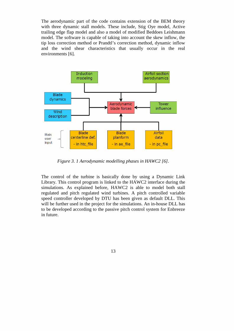
The aerodynamic part of the code contains extension of the BEM theorywith three dynamic stall models. These include, Stig Oye model, Activetrailing edge flap model and also a model of modified Beddoes Leishmannmodel. The software is capable of taking into account the skew inflow, thetip loss correction method or Prandtl’s correction method, dynamic inflowand the wind shear characteristics that usually occur in the realenvironments [6].

Figure 3. 1 Aerodynamic modelling phases in HAWC2 [6].

The control of the turbine is basically done by using a Dynamic LinkLibrary. This control program is linked to the HAWC2 interface during thesimulations. As explained before, HAWC2 is able to model both stallregulated and pitch regulated wind turbines. A pitch controlled variablespeed controller developed by DTU has been given as default DLL. Thiswill be further used in the project for the simulations. An in-house DLL hasto be developed according to the passive pitch control system for Enbreezein future.

14

3.1 Nimbus 5.2 1.6 KW wind turbine

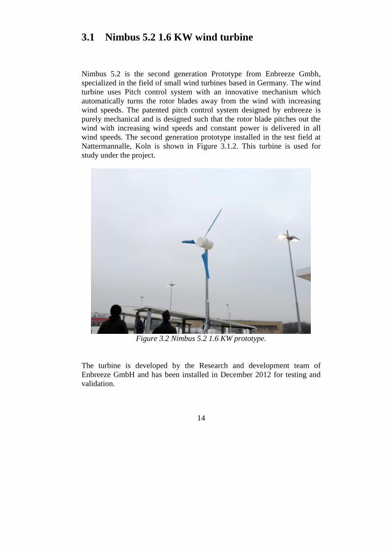
Nimbus 5.2 is the second generation Prototype from Enbreeze Gmbh,specialized in the field of small wind turbines based in Germany. The windturbine uses Pitch control system with an innovative mechanism whichautomatically turns the rotor blades away from the wind with increasingwind speeds. The patented pitch control system designed by enbreeze ispurely mechanical and is designed such that the rotor blade pitches out thewind with increasing wind speeds and constant power is delivered in allwind speeds. The second generation prototype installed in the test field atNattermannalle, Koln is shown in Figure 3.1.2. This turbine is used forstudy under the project.

Figure 3.2 Nimbus 5.2 1.6 KW prototype.

The turbine is developed by the Research and development team ofEnbreeze GmbH and has been installed in December 2012 for testing andvalidation.

15

The specifications of the turbine are shown in the Table 3.1 below

Table 3.1 Specifications of Nimbus 5.2.

Properties Nimbus 5.2 Enbreeze

Rated Power 1.6 KW

Rated speed 7 m/s

Cut in wind speed 3 m/s

Design wind class II (DIN EN 61400-2)

Rotor diameter 5 m

Rotor type Down wind

Blade Material PET

ControlMechanical Pitch

control

Rotor swept area 20 m2

Direction of rotationClockwise in the down

wind direction

Number of blades 3

Pitch angle Variable

Yaw system Passive

Nacelle Tilt 0 degree

Teetering in rotor Non teetered type.

Coning angle 0 degree

Generator Permanent magnetgenerator

Tower height 6 m

Tower top mass 151.2 kg

Tower base diameter 152.4 mm

16

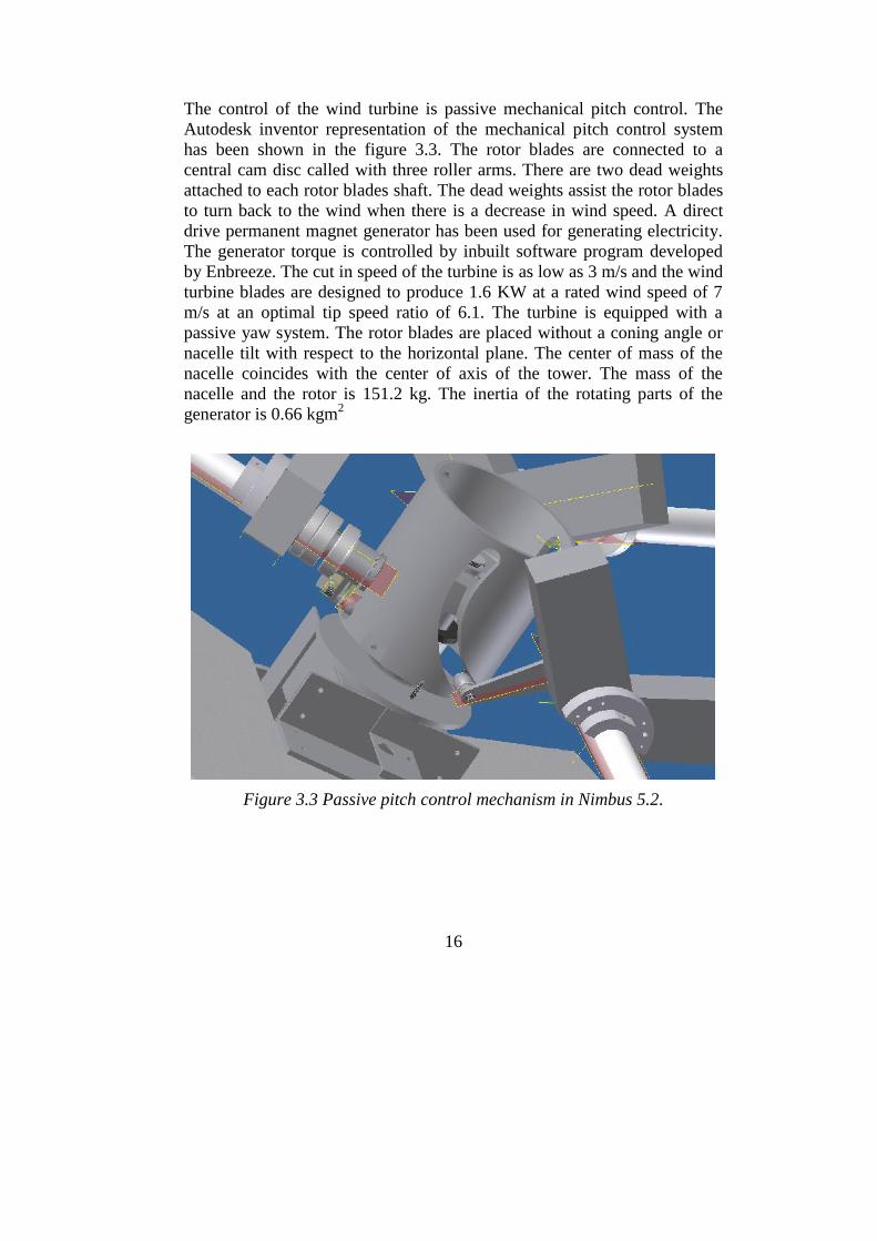
The control of the wind turbine is passive mechanical pitch control. TheAutodesk inventor representation of the mechanical pitch control systemhas been shown in the figure 3.3. The rotor blades are connected to acentral cam disc called with three roller arms. There are two dead weightsattached to each rotor blades shaft. The dead weights assist the rotor bladesto turn back to the wind when there is a decrease in wind speed. A directdrive permanent magnet generator has been used for generating electricity.The generator torque is controlled by inbuilt software program developedby Enbreeze. The cut in speed of the turbine is as low as 3 m/s and the windturbine blades are designed to produce 1.6 KW at a rated wind speed of 7m/s at an optimal tip speed ratio of 6.1. The turbine is equipped with apassive yaw system. The rotor blades are placed without a coning angle ornacelle tilt with respect to the horizontal plane. The center of mass of thenacelle coincides with the center of axis of the tower. The mass of thenacelle and the rotor is 151.2 kg. The inertia of the rotating parts of thegenerator is 0.66 kgm2

Figure 3.3 Passive pitch control mechanism in Nimbus 5.2.

17

3.2 Aerodynamic Modelling

Aerodynamic models are implemented using different aerodynamic theoriesin fluid mechanics such as

Blade Element Momentum theory

Free wake panel method

Among these two, Blade element theory is most widely used because of itscomputational easiness and accurate results with less input. The BEMtheory is discussed below.

3.2.1 Blade Element Momentum Theory

The blade element theory can be used in the aerodynamic modeling of therotor blades. The blade is divided into a number of cross sections along thelength of the blade and the each 2D element is analyzed. The lift and dragin each section along with the thrust and the torque is balanced. Besides theforce balance, the equilibrium of momentum is also considered. Both axialmomentum and angular momentum are applied. The balance of rate ofchange of fluid momentum with the blade forces is established for eachannular area [7].

The lift acting on the wind turbine is given by the equation,

LhubcCVL 2

2

1 (3.1)

The drag force can be found out from the equation,

18

D= DhubcCVL 2

2

1 (3.2)

The rotor blade profiles starts stalling at an angle of attack of 12-15 degreedepends upon the aerodynamic profile and the position of the profile in thespan of the rotor blade. This is due to the increase in turbulence in the upperpart of the blade which decreases lift and increases drag. The force balanceon an airfoil according to the BEM theory is shown in Figure 3.4

Figure 3.4 Force balance on an aerofoil according to BEM [7].

Figure 3.5 Velocity triangle at the aerofoil section [7].

19

The fraction of annular area covered by the control volume is

r

Nrc

2

)( (3.3)

where c(r) is the chord length at the radius r, N, number of blades

r, the radius of the rotor blades.

The Thrust and Torque on the control volume is given by

dT = NFN dr =2

2

sin

)1(

2

1

drcCaUN N (3.4)

where dT is the is the thrust in N ,U∞ is the free stream velocity in m/s, Nis the number of blades, a is the tangential induction factor

FN and FT are the forces per unit length in N/m

dQ= rNFT dr =

cossin

)1()1(

2

1 rdrcCaraU T (3.5)

The two induction factors are defined as

a=1

))(sin(sin41

NC

(3.6)

a'=1

))(cos(sin41

TC

(3.7)

20

tan =)1(

)1(

ar

aU

(3.8)

These set of non linear equations are solved numerically. The blade elementtheory provides accurate results in comparison to the cost of time spent oncomputation. Each control volumes are assumed to be independent andeach strip is computed for the results before starting the computation of thenext radius.

3.2.2 Free wake panel method.

Free wake panel method is another method used for aerodynamic modeling.Free wake modeling is used when the flow is subsonic and viscous effectsare negligible. The method is generally used in aerospace industry forconceptual analysis because of its easiness and less time required for theresults.

Panel method can be used to predict the lift and form drag. It cannot modelviscous effects like boundary layers and flow separation. The Skin Frictiondrag cannot be calculated by this method. A wake is generated on thetrailing edge of the aerofoil for the calculation of lift and drag, The methodis incapable of calculating the lift and the form drag without the wake dueto its inviscid modeling nature.

3.2.3 Aerodynamic modeling in HAWC2

Aerodynamic modeling in HAWC2 uses the classic Blade ElementMomentum theory approach to model the aerodynamic forces acting on theblade. The aerodynamic forces acting on the structure includes the forcesacting on the blades as well the aerodynamic drag forces acting on the

21

tower and the nacelle. The forces are the transferred to the structural modelto calculate the aeroelastic response. The aerodynamic input to HAWC2 isdistributed in 3 main files.

Center line definition of the blade in .htc file

The Profile coefficients (Polars) of the rotor blades sections in the.pc file

The data of the blade Plane form in the .ae file.

The profile coefficients of the blades are obtained by a 2D CFD simulationof the rotor blades. The center line of the blades is defined with respect tothe global coordinates the structural file. The thickness to chord lengthration along the span of the blade is calculated for respective sections and iswritten inside the .ae file.

The aerodynamic modeling in HAWC2 is able to predict the dynamicinflow which occurs when the wind load changes are faster than the timeneeded for the inflow velocity to be in equilibrium with the aerodynamicloads. The design for the skew inflow will take care of the real cases with ayaw misalignment such that the flow is not always axisymmetric. The sheareffects on the blade due to different wind speeds with respect to bladesection height from the ground are taken care into account using a polargrid induction model. When there is very large displacement of the end ofthe rotor blades such that the rotor blades are not perfectly rotating in therotor plane, the thrust on the rotor blades changes and so the inducedvelocities. This effect is considerable in modeling very large wind turbineblades. Prandtl's tip correction model has to overcome BEM theory'sassumption of having infinite number of blades. Glauert's yaw correctionformula is used to derive the resultant induction factors in different yawmisalignment cases [6].

The BEM procedure used in HAWC2 is implemented by discretizing therotor plane into independent concentric annular elements and azimuthalvariation of loading.

The local wind speed is obtained at each point of the polar grid andthe local induced wind speed from the previous iteration is used forthe calculation.

22

The local coefficient of thrust is calculated at two neighboringblades which has the local wind speed and the local induction used.

The Prandtl's tip loss factor which take care of the assumption ofinfinite number of blades in BEM theory has been rectified

The local CT is obtained by interpolating the CT based on 2 bladesand the azimuthal distance between the wind speeds.

The local induction factor 'a' is obtained at the point.

The correction for skew inflow angle is added to the inductionfactor

The tangential induction factor is then calculated

The axial and tangential induction factors are then calculated.

In accordance with the skew inflow angle and axial inductioninfluence, a correction is made for the azimuthal variations of axialinduction.

The tangential u and axial u are updated based on two first orderlow pass filters. This is done such that both near and far wake [8].

These steps are done for each point in the polar grid, after this for eachpoint in the blade the induced velocities are calculated at a radius byazimuthal interpolation of two closest grid points.

3.2.4 Determination of Polars of rotor blade airfoil Profiles

The Aerodynamic part of HAWC2 works on BEM theory. The blade isdefined as different sections starting from the tip of the blade to the rotorcentre. The structural properties, the aerodynamic coefficients and theaerodynamic layout are defined in 3 different data sheets and are linked tothe HAWC2 program.

The aerodynamic layout file contains the data for defining the rotor bladeprofile with respect to the Z axis which starts the last node of the hub. The

23

position of the aerodynamic centre is kept at C1/4 of the Chord, where C isthe chord length with calculated velocities in C3/4 as shown in figure 3.6and in Figure 3.7.

Figure 3.6 Definition of aerodynamic centre on aerofoil section [6].

Figure 3.7 Forces and angle velocity on the rotor blades.

24

3.2.5 Enbreeze Rotor blades

The rotor blades used in the wind turbine has been developed by thecompany named Aerodesign works. It of 2.5 m in diameter and isfabricated with PET. The rotor blades are designed for a rated Power of 1.6KW at 7 m/s. The HAWC2 aerodynamic input requires the Polars of therotor blade from angles of attack range from -180° to +180 ° degrees. Thelift and drag coefficients of the rotor blades at different angle of attack arefound out using Solid works flow simulation student version. Various 2Daerofoil analysis softwares likes Java foil, Aerofoilengineering, X foil, andQblade where used to for the same and the results have been tested for thelift and drag coefficients available and it is found that Solidworks flowsimulation has more stability and better results especially near the stallregion. The simulation setup has been validated for a NACA airfoil and theresults were obtained with an error of ±5 %.

Five Profile sections along the length is selected as shown in the Figure 3.8.

Figure 3.8 Aerofoil sections under analysis at different parts of the blades.

25

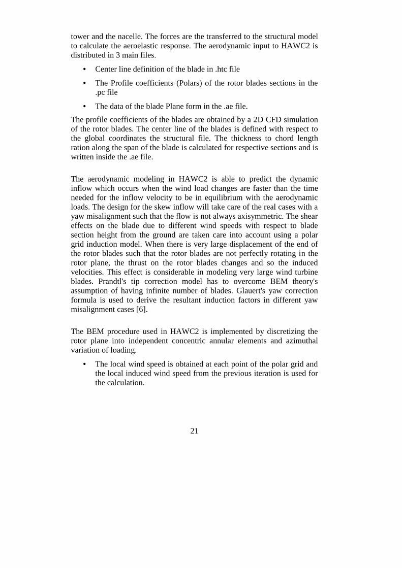
An initial computational mesh of 400*300 is created. A local mesh iscreated in the interface where solid and fluid cells interact. A very highmesh refinement level is given to capture the change in properties wherethe solid and fluid interact as shown in Figure 3.9.

Figure 3.9 Refined partial cells at solid fluid interface.

Symmetric boundary conditions are given at both ends of the Z axis whichis necessary for 2 D flow. The inlet velocity for each section is calculatedbased on a constant Reynolds number. The Reynolds number selected forthe flow is Re=300,000. The inlet velocities for each section are calculatedfrom the formula

vL

Re (3.9)

where Re is the Reynolds number

v is the velocity in m/s

l is the length in m

μ is the kinematic viscosity in Ns/m2

The inlet velocities are defined such that the flow is towards the positive xdirection, and the solid fluid interaction begins at the leading edge and

26

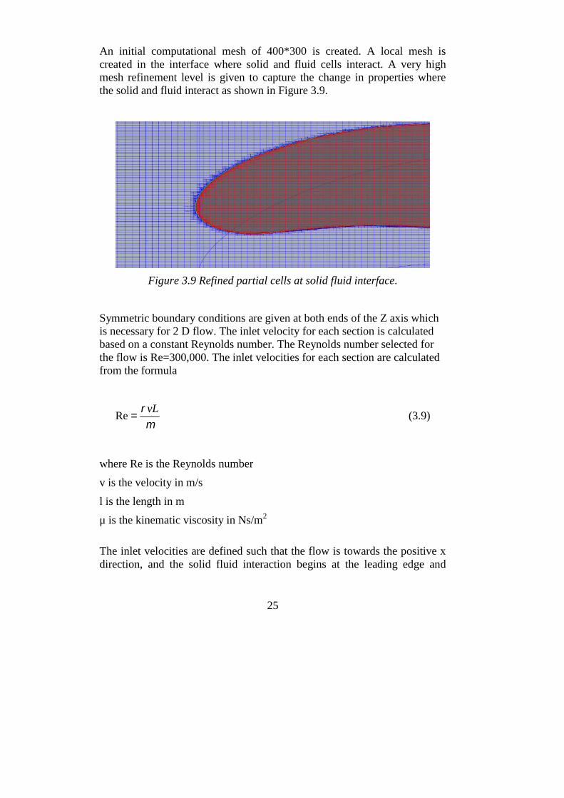
leaves the rotor blade at the trailing edge. A turbulence intensity of 0.1 %and turbulence length of 10 micro meters are selected. The resultant forceson the x direction are equal to the Drag force of the profile and the force inthe y direction is equal to the Lift force. The coefficient of lift and drag arecalculated from the following equations written below. 5 Sets of Batchsimulations were done for different angle of attack starting from 0 to 90degrees. Each batch simulations included 20 simulations. The coefficient oflift versus angle of attack is shown in Figure 3.10 below. It can be seen thatthe most of the rotor blade sections stall at an angle of attack of 18 -20degrees.

Figure 3.10. CL versus angle of attack, section 11

3.3 Structural Definition

Aeroelastic simulation includes aerodynamic and structural simulations.The dynamics of the operation of wind turbine can be understood by thestructural modelling of the HAWT in Multibody dynamics. It can be alsounderstood as floating frame approach. The wind turbine structure isdivided to a number of elements. Each element is considered as aTimoshenko beam element which accounts for both shear and bendingdeformation. Each body has its own coordinate system. The calculation ofinertial loads is based on this coordinate system when the body is moved inspace. This gives the advantage of accommodating for large deflections androtations which is hard to be visualised in FEM method [9].

27

Each element interacts with the neighbouring elements with joints. Theconstraints are imposed in these joints and are implemented as algebraicequations. The HAWC2 is designed such that external loads are applied onthe deformed state and this is very useful in analysing pitch loads and twistof the blades [9]. When the elements are divided accordingly, HAWC2 willbe able to simulate large rotations and also the wind turbine with highlyflexible structures.

3.4 Definition of Tower and Nacelle Components

The main structural components such as Tower, the connection between thetower and the Nacelle, the Yaw bearing, the main rotating shaft and thehub, pitch bearing between the hub and the rotor blades and the rotor bladeshas to be modelled for the aeroelastic analysis of the turbine. The HAWC2models the structural components as Timoshenko beam elements withdefined Centre line of the each components with reference to the local andglobal coordinate system. The definition of the centre line is the first andforemost part of the structural definition. Each structural part is defined asTimoshenko beam element with 19 Structural properties shown in the table3.2. The representation of elements and nodes used in my model is shownin Figure 3.11.

All bodies are modelled as Timoshenko beam elements with 6 Degrees ofFreedom. These 19 parameters define the Timoshenko beam inputparameters for the calculations and these have to be calculated with respectto each node in the each structural body. The structural and materialdamping for these beam elements are also given in the .htc files. Theorientation of each node is also given as input with correspondingconstraints for motion.

Multibody dynamics is used in the structural modelling which uses thefloating frame approach of the reference point. Large deflections(translations) and rotations are calculated on the points where the nodes ofthe main body structures interact while small deflection is calculated withineach main body nodes [9]. The joints for each main body structure havecoupled with each other using algebraic equations. This helps to model nonlinearity like large deflection and rotations being passed from one main

28

body to an another body. The floating frame approach can be visualised inFigure 3.12

3.11. Multibody formulations, elements and nodes in the structure.

29

Table 3.2.1 Structural input for HAWC2.

Value

rCurved length distance from themain_body node 1[m].

m Mass per unit length kg/m

xm, ymxc2 and yc2 coordinate from C1/2 tomass centre [m].

rixRadius of inertial related to elasticcentre.

riyRadius of inertial related to elasticcentre.

xs, ys xc2 and yc2 coordinate from C/2 toshear centre[m].

E Modulus of elasticity, N/m2.

G Shear modulus of elasticity, N/m2.

Ix Area moment of inertia with respect tothe principal bending xe axis [m4].

Iy Area moment of inertia with respect tothe principal bending ye axis.

K Torsional stiffness constant with respectto the ze axis at the shearcentre.[m4/rad].

kx Shear factor for force in principalbending xe direction.

ky shear factor for force in principalbending ye direction

A cross sectional area[m2]

Ɵs Structural pitch with respect to zc2 axis.

xe, ye xc2, yc2coordinate from C1/2 to centreof elasticity[m].

30

Fig. 3.2.2.1 Multibody dynamics approach.

Modelling of the wind turbine is done by breaking down the wind turbine tomain bodies and sub structures. The main bodies in the enbreeze Nimbus5.2 include

Tower.

Connection between tower and Nacelle.

Main rotor shaft.

Hub.

Connection between hub and the rotor blades.

Rotor blades.

Each main body can be divided into a number of sub bodies or substructures. Main bodies are linked to each other with joints.

31

Figure. 3.13. Definition of beam element nodes

The properties of the main bodies are first defined with respect to its owncoordinate system. Each bodies has its own coordinte systems. Thesecoordinate systems have its own orientation with respect to the globalcoordinate system.

32

The tower of enbreeze Nimbus 5.2 is 6 m long in length. The tower ismodeled with 8 elements with the first node of the first element being fixedto the ground and the last element of the 8th node which is connected to theconnection element between the tower and the nacelle. The base node or thefirst node of the tower is fixed and attached to the ground using fix 0constraint in HAWC2 which restricts both translation and rotation at node1. The global coordinate system is kept such that negative x is pointingtowards the increasing tower height and negative y in the direction of windin our down wind case. The structural properties above mentioned in Table3.2 has been calculated for each section and has been updated in the .st filein the HAWC2 data section.

The connection between the tower top and the nacelle is defined with oneelement consisting of the first node attached to the tower top and the secondone at the beginning of the rotating shaft. The Nimbus 5.2 consists of arotary flange with the bearing block which consists of the yaw bearing andsuitable structures for accommodating the slip rings and the othercomponents for instrumentation. The connecting structure is modeled as asingle structure with one beam element. The connecting block is 200 mlong and has the same direction of xyz coordinates as the global case andthe node connecting the tower, but rotated along the x axis with an angle of-90 degrees and the rotated at an angle of 180 degrees on the y axis on thenode connecting to the shaft. The change in orientation at different nodalpoints can be seen in the figure 3.15 below. The second node of this beamelement where the first node of the shaft is attached is the place where themass of the nacelle and inertia of the nacelle is given. The inertia of thestructure is calculated using Autodesk Inventor with respect tocorresponding orgin from the CAD files used in the design and productionprocess.

The main body, the rotor shaft of the wind turbine which connects therotating rotor blade hub to the generator is modeled as a Timoshenko beamwith 5 elements. The shaft is 0.5 m long in our case. The first node of thebeam element of the shaft which links the connection between the shaft andthe tower intermediate structure has given the generator inertia and the lastnode of the 5 beam element has given the mass of the rotating parts whichinclude the hub, the rotor blades, 3 in our case and the dead weights whichare used to assist the rotor blades in the control system when the windspeed decreases so that the rotor blades pitches back to the wind. There are

33

2 bearing in our case, the main rotating shaft bearing and also a bearing inthe middle of the shaft for better stability and also connecting componentslike flexible couplings attaching the rotor shaft and the generator shaft.These components are not directly modelled in our case, but added with thegenerator mass and inertia to consider the effects of the extra mass andinertia of these components. The orientation of the coordinate system ischanged at the last node of the shaft to model the rotor plane. Thecoordinates from the tower top is rotated 90 degrees in the anticlockwisedirection with respect to x axis and then rotated 180 degrees clock wise.

The hub of the enbreeze wind turbine consists of the innovative pitchcontrol system and suitable connection mechanism to connect the rotorblades to the hub. The control of the wind turbine is mechanical pitching ofthe rotor blades in a cam disc. The control of the system has to modelled ina suitable program like C++ or Python and to be linked to the HAWC2program. This has not been done due to the time and economic constraintsat the moment. In the HAWC2 structural input the hub is defined as a mainbody. Three hubs are defined for a 3 bladed wind turbine as a main bodies,with one beam element each. The first node of each hub element is attachedto the last node of the shaft and the second node to the rotor blades.

The coordinates from the tower top is rotated 90 degrees in theanticlockwise direction with respect to x axis and then rotated 180 degreesclock wise for the first hub. For the second and third hub the coordinatessystems from the tower top are then rotated 90 degrees in anticlockwisedirection with respect to y axis and then rotated 60 degree anticlockwisewith respect to the y axis to accommodate 120 degree angle between the 3rotor blade axes. The hub is made of aluminum. The beam elementrepresentation of the whole structural representation can be seen in theFigure 3.13. The eccentricity of the position of rotor blades in coinciding tothe central point in the rotor axis is shown by the Figure 3.14. This featurehelps to reduce the flap wise bending moment in the rotor blades.

The pitching axis of the wind turbine rotor blades are designed such theyusually coincide at the centre of the rotating axis. In our case the axis ofeach rotor blades are kept at an eccentricity of 0.1 m from this axis. Thisfeature has been modeled using suitable function in the HAWC2.

34

Figure 3.14 Hub, Nimbus 1.6 KW Autodesk inventor view.

The rotor blades are attached to the hub. The main body rotor blades aredesigned with 7 beam elements across the length of the rotor blades. Theblades are 2.5 m in length and which consists of cylindrical structure withall the necessary components like flying weights and suitable connectionmechanisms till 1 m and then 1m to 2.5 m composes blade profiles. Theblades are designed for very small wind speeds with an optimal tip speedratio of 6.1. The cut in speed of the rotor blades are as slow as 3 m/s and theoptimal wind speed is 7 m/s, producing a power of 1.6 KW.

The orientation of the coordinates of the rotor blades are similar to the lastnode of the respective hubs they are connected with. The rotor blades of thedown wind turbines are usually provided with a coning angle. The coningangle is the angle between the pithing axis of the rotor blade with respect tothe rotor plane. Studies has showed that coning angle helps the down windturbine to align better with the wind when the wind changes it direction.The coning angle is given 0 degree in our case for preliminary analysis andthe wind turbine nacelle is at 0 degree tilt with respect to the horizontalplane. The structural properties of rotor blades are accurately obtained

35

using a Beam Cross Section Analysis Software called BECAS from DanishTechnical Institute.

Fig. 3.15. Local coordinate system and orientation of main bodies.

The structural properties of each and every body with respect to its localcoordinates and global coordinates have been calculated. As discussedbefore, BECAS is used for complex structures like rotor blades, but for restof the parts it is calculated using basic equations. The orientation of thelocal coordinates at different main bodies is shown in the Figure 3.15. Thecalculation of structural properties of shaft is shown below

mmD 4.152 (3.10)

36

m0.0762=R (3.11)

mm6.3=t (3.12)

mm0.0699=t-R=r (3.12)

37850

m

kg (3.13)

21110.2

m

NEE (3.14)

2108.8

m

NEG (3.15)

20028916.0 mA (3.16)

m

kgAm 6991886.22 (3.17)

444 0000077.0)(4

mrRI x

(3.18)

xIyI (3.19)

42ix 0000077.0R m

A

I x (3.20)

37

42iy 0000077.0R m

A

I x (3.21)

5.0k y xk (3.22)

444 0000155.0)(2

mdDK

(3.23)

Similarly the structural properties are calculated for 8 sections of Tower,one section of tower top, 5 sections of the shaft, 2 sections of each hub.BECAS has been used to find the structural properties of the blades.

Figure 3.16 Definition of blade center lines [6].

38

3.4.1 BECAS

The cross sectional analysis tool called BECAS is used for the sectionanalysis of special structures like rotor blades. The elastic centre, the shearcentre and the mass centre can be determined by the same.

Rotor blades are one of the most important structural elements which haveto be evaluated in the aeroelastic modelling. The static, dynamic andaerodynamic forces acting on the rotor blades make the analysis difficultand time consuming. The material used in most light weight rotor bladesincludes non linear materials like fibre glass or other reinforced plastics.The structural properties depends upon various factors like the materialorientation, the number of layers, the orientation of layers and also the waythe rotor blades are fabricated.

For the analysis of long and slender structures like rotor blades, beammodels are more accurate and computationally efficient compared to that ofusing shell or solid models [10]. The software used for the cross sectionalanalysis is called BECAS, Beam Cross section Analysis Software fromDanish Technical University is used for the same. The software is able tohandle arbitrary cross section geometries, anisotropic materials and materialinduced couplings.

A finite element beam model of the rotor blade sections has been createdusing BECAS. 7 Sections are selected along the length of the rotor bladesfor analysis. The rotor blade sections are taken as the same radius lengthused for finding the Polars such as coefficient of lift, coefficient of drag andcoefficient of Pitch moment used in Solid works flow simulation.

BECAS is a MATLAB based code. The post processing is done inMATLAB. There are two pre-processing tools used to generate input forBECAS. The steps in the process of modelling the aerofoil on BECAS canbe explained as in Figure 3.17

39

Fig 3.17 BECAS steps[12]

3.4.2 Airfoil2Becas

Airfoil2BECAS is a python based script used to generate input to BECAS.It is a pre processing tool which works on NumPy which is numericalPython. The same 7 sections along the length of the rotor blades has beenchosen for analysis. Apart from the airfoil coordinate data which definesthe x and y position which in turn defines the shape, the layup informationof the position of fibres and the material used for the fabrication of rotorblades.

The program generates 2D mesh in the airfoil for the analysis in BECAS inthe suitable format. 9 key points are defined in between the airfoilcoordinates which divides each airfoil section to 8 regions. There is apossibility to assign different material orientation and material propertiesfor different sections. Shear webs are used by wind turbine manufacturersto stabilise the rotor blades and also to decrease the thickness of thefabricating material. A number of shear webs can be defined between thenodal points based on the design of the rotor blades and correspondingmaterial properties are assigned in the airfoil2becas.py python script.

40

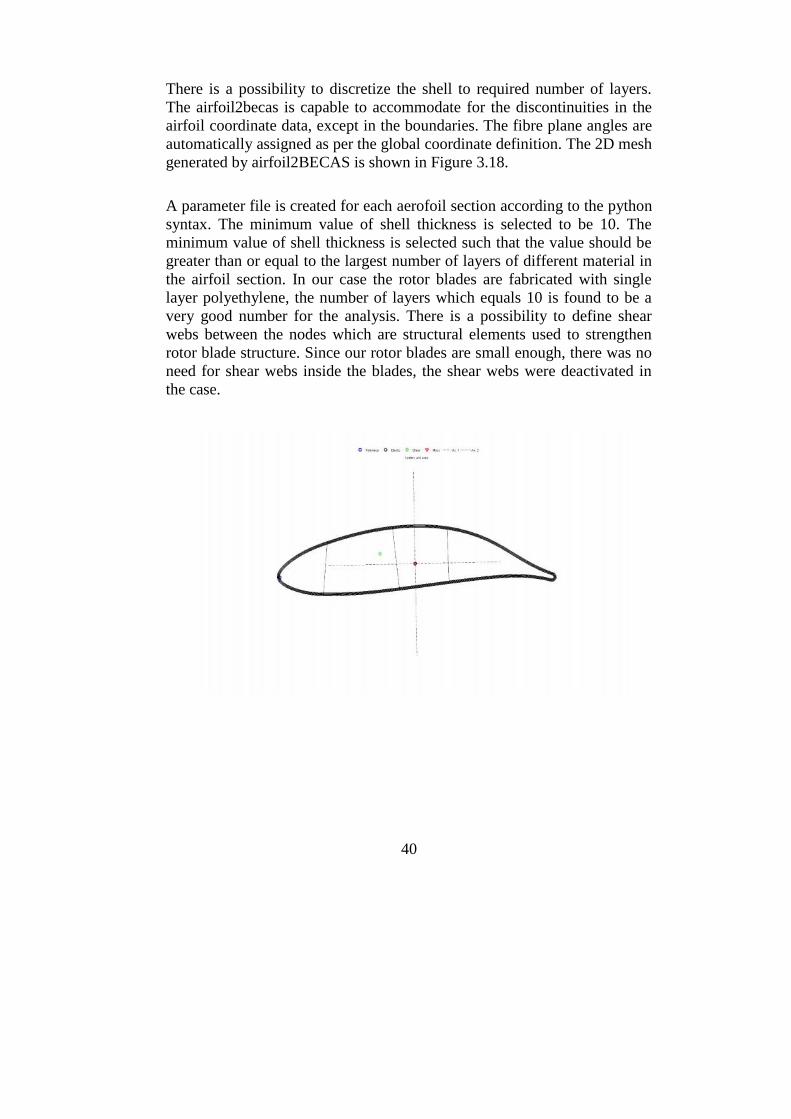
There is a possibility to discretize the shell to required number of layers.The airfoil2becas is capable to accommodate for the discontinuities in theairfoil coordinate data, except in the boundaries. The fibre plane angles areautomatically assigned as per the global coordinate definition. The 2D meshgenerated by airfoil2BECAS is shown in Figure 3.18.

A parameter file is created for each aerofoil section according to the pythonsyntax. The minimum value of shell thickness is selected to be 10. Theminimum value of shell thickness is selected such that the value should begreater than or equal to the largest number of layers of different material inthe airfoil section. In our case the rotor blades are fabricated with singlelayer polyethylene, the number of layers which equals 10 is found to be avery good number for the analysis. There is a possibility to define shearwebs between the nodes which are structural elements used to strengthenrotor blade structure. Since our rotor blades are small enough, there was noneed for shear webs inside the blades, the shear webs were deactivated inthe case.

42

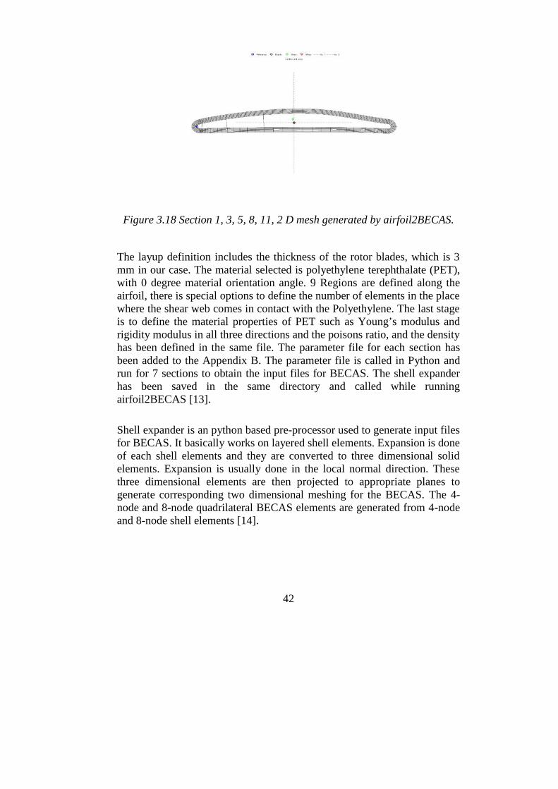
Figure 3.18 Section 1, 3, 5, 8, 11, 2 D mesh generated by airfoil2BECAS.

The layup definition includes the thickness of the rotor blades, which is 3mm in our case. The material selected is polyethylene terephthalate (PET),with 0 degree material orientation angle. 9 Regions are defined along theairfoil, there is special options to define the number of elements in the placewhere the shear web comes in contact with the Polyethylene. The last stageis to define the material properties of PET such as Young’s modulus andrigidity modulus in all three directions and the poisons ratio, and the densityhas been defined in the same file. The parameter file for each section hasbeen added to the Appendix B. The parameter file is called in Python andrun for 7 sections to obtain the input files for BECAS. The shell expanderhas been saved in the same directory and called while runningairfoil2BECAS [13].

Shell expander is an python based pre-processor used to generate input filesfor BECAS. It basically works on layered shell elements. Expansion is doneof each shell elements and they are converted to three dimensional solidelements. Expansion is usually done in the local normal direction. Thesethree dimensional elements are then projected to appropriate planes togenerate corresponding two dimensional meshing for the BECAS. The 4-node and 8-node quadrilateral BECAS elements are generated from 4-nodeand 8-node shell elements [14].

43

Figure 3.19 Finite element shell model in BECAS [14]

The advantage o the beam part is that it is more accurate in predicting theglobal displacements and computationally efficient compared to the shellelements. The BECAS assumes the deformation of the body as acombination of rigid body motions and also warping displacements. Theprinciple of virtual work is used in the formulation of finite elementequations. The three dimensional warping displacements are discretizedusing two dimensional finite elements. The output from BECAS can bedirectly taken to HAWC2.

The BECAS2HAWC2 matlab function is capable of giving these 19calculated values at each section of the rotor blade to the tip section. Thesevalues are taken to the structural definition file of HAWC2 for the rotorblades. BECAS calculations have been done for 7 sections along the lengthof the rotor blade from the centre to the tip. The output fromairfoil2BECAS and shell expander is the input files to BECAS. 7Simulations have been done and the results are exported to HAWC2structural file.

44

3.5 Definition of wind

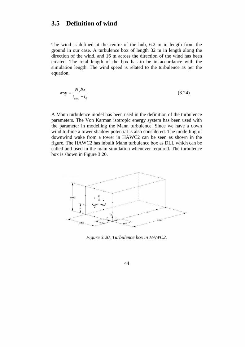
The wind is defined at the centre of the hub, 6.2 m in length from theground in our case. A turbulence box of length 32 m in length along thedirection of the wind, and 16 m across the direction of the wind has beencreated. The total length of the box has to be in accordance with thesimulation length. The wind speed is related to the turbulence as per theequation,

0tt

xNwsp

stop

x

(3.24)

A Mann turbulence model has been used in the definition of the turbulenceparameters. The Von Karman isotropic energy system has been used withthe parameter in modelling the Mann turbulence. Since we have a downwind turbine a tower shadow potential is also considered. The modelling ofdownwind wake from a tower in HAWC2 can be seen as shown in thefigure. The HAWC2 has inbuilt Mann turbulence box as DLL which can becalled and used in the main simulation whenever required. The turbulencebox is shown in Figure 3.20.

Figure 3.20. Turbulence box in HAWC2.

45

For 7 m/s wind speed the turbulence box is created with the followingdimensions, Number of points in the x direction=1024 with Δx is0.41015625. The wind created for the simulation is shown in Figure 3.21.

Figure 3.21. 7 m/s wind inside the turbulence box.

46

4 Simulation and Natural frequencyAnalysis

The dynamic response to a system to an excitation depends upon the naturalfrequency of the system and the damping present in the structures. Thestructural security of a wind turbine can be increased using stiff structures,but the production costs of main components like tower and rotor bladeswill increase the production cost. The aeroelastic modelling of the turbinegives the understanding about the structural dynamic response of the windturbine under various forces of excitation when the wind turbine isoperating the under various environmental conditions. This make the designengineers to choose more flexible, light weight structures in designing thewind turbine which makes the wind energy more economical.

The response of a structure when subjected to an external excitation forcecan be of three types [15].Quasi static, when the frequency of excitation ofthe system is well below the natural frequency of the wind turbine. In thiscase the response of the system will be similar to the excitation force butwith a phase lag. Resonance happens when the frequency of excitation iscloser to the natural frequency of the system, within a narrow region wherethe wind turbine response may be several times magnified compared toresponse under static load case. This can even lead to catastrophic failuresof the wind turbine since the magnitude of amplification of the responsewill be very high and unpredictable.

The amplitude depends upon the damping of the structure since both theinertial and spring forces cancel each other. When the excitation frequencyis way above the natural frequency of the structure the mass will not be ableto respond to the frequency causing a low response. The response of systemto the same force applied at different frequencies of excitation is shown inFigure 4.1, Figure 4.2 and Figure 4.3. In dynamics the frequency of load isas important as the magnitude of the loads. In case of wind turbine, itexperiences time varying loads in different wind conditions. The responseof the wind turbine as we can see from the figure to a particular type ofexcitation will be similar to excitation of the force but with a differentmagnitude and phase.

47

Figure 4.1. Quasi static response Solid Line F(t), Dashed line Response.

Figure 4.2 Resonance Solid line: F(t) Dashed line: Simulated response.

Figure 4.3 Inertia dominated response line: F(t) Dashed line: Simulatedresponse [15].

48

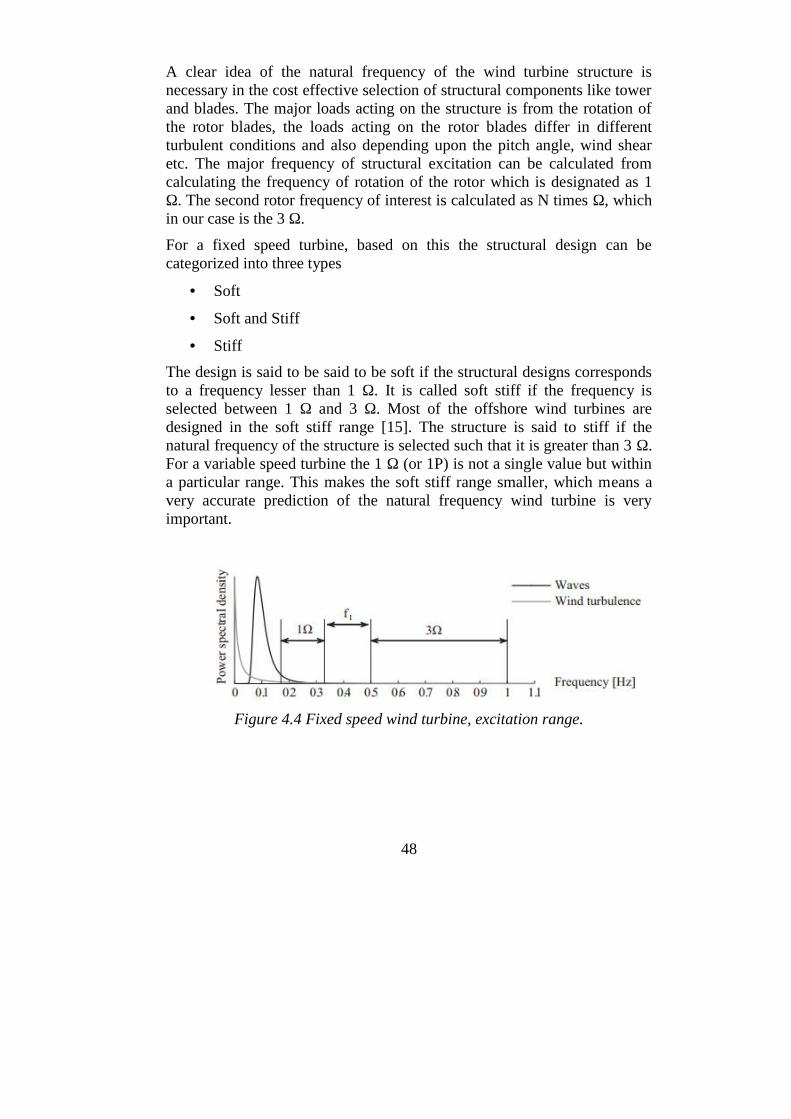
A clear idea of the natural frequency of the wind turbine structure isnecessary in the cost effective selection of structural components like towerand blades. The major loads acting on the structure is from the rotation ofthe rotor blades, the loads acting on the rotor blades differ in differentturbulent conditions and also depending upon the pitch angle, wind shearetc. The major frequency of structural excitation can be calculated fromcalculating the frequency of rotation of the rotor which is designated as 1Ω. The second rotor frequency of interest is calculated as N times Ω, whichin our case is the 3 Ω.

For a fixed speed turbine, based on this the structural design can becategorized into three types

Soft

Soft and Stiff

Stiff

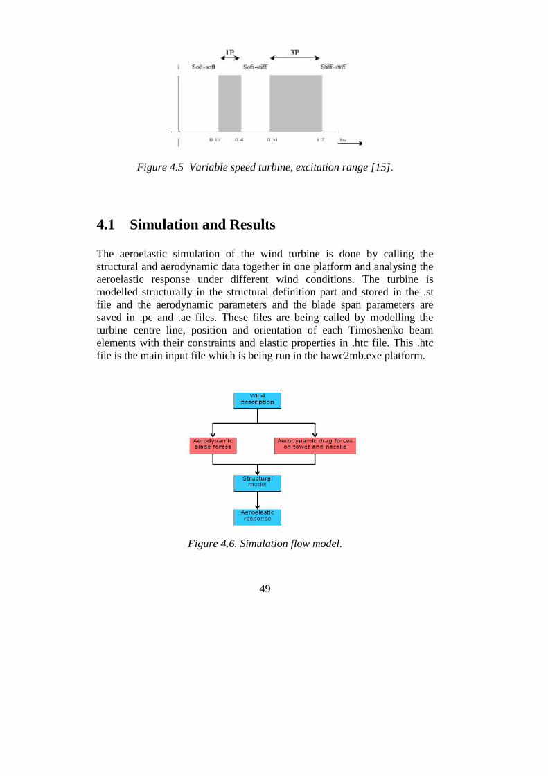
The design is said to be said to be soft if the structural designs correspondsto a frequency lesser than 1 Ω. It is called soft stiff if the frequency isselected between 1 Ω and 3 Ω. Most of the offshore wind turbines aredesigned in the soft stiff range [15]. The structure is said to stiff if thenatural frequency of the structure is selected such that it is greater than 3 Ω.For a variable speed turbine the 1 Ω (or 1P) is not a single value but withina particular range. This makes the soft stiff range smaller, which means avery accurate prediction of the natural frequency wind turbine is veryimportant.

Figure 4.4 Fixed speed wind turbine, excitation range.

49

Figure 4.5 Variable speed turbine, excitation range [15].

4.1 Simulation and Results

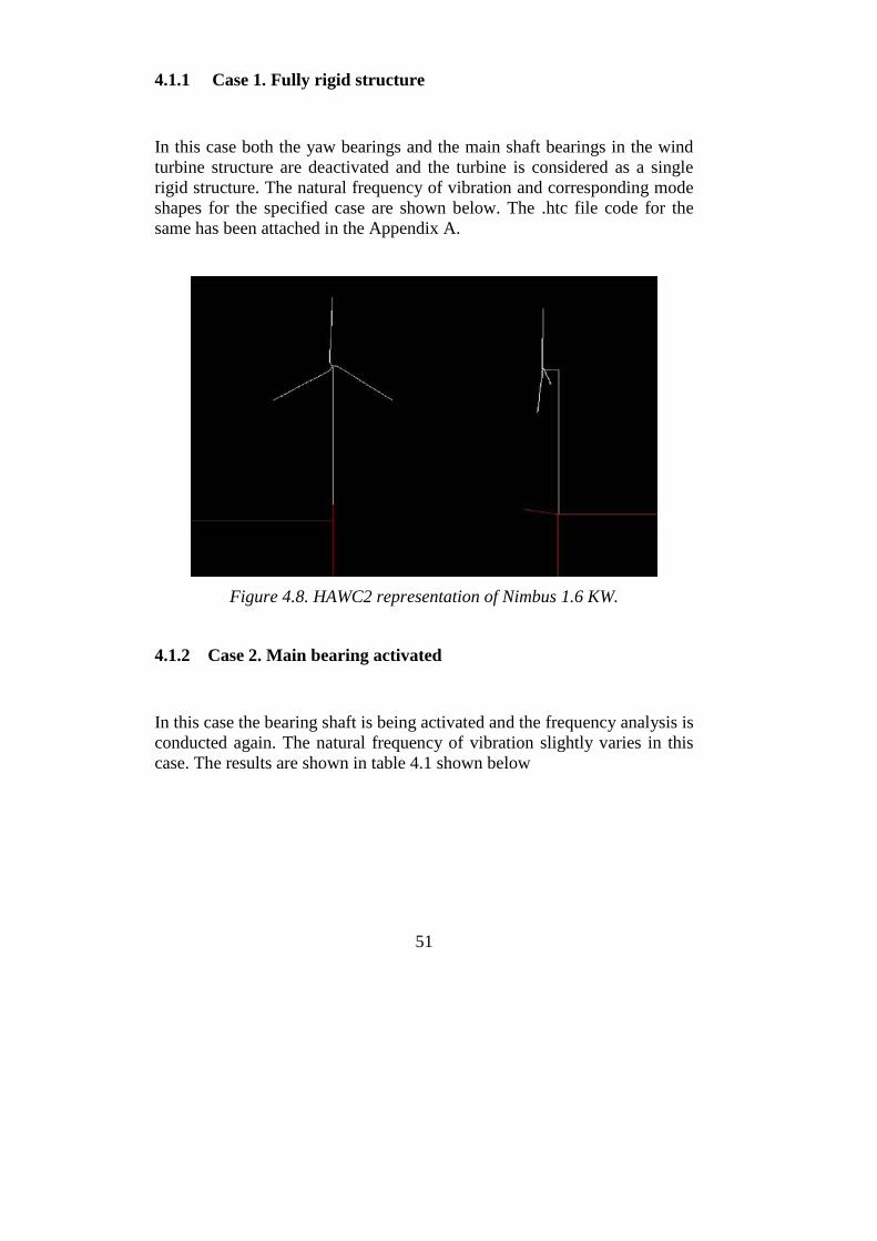
The aeroelastic simulation of the wind turbine is done by calling thestructural and aerodynamic data together in one platform and analysing theaeroelastic response under different wind conditions. The turbine ismodelled structurally in the structural definition part and stored in the .stfile and the aerodynamic parameters and the blade span parameters aresaved in .pc and .ae files. These files are being called by modelling theturbine centre line, position and orientation of each Timoshenko beamelements with their constraints and elastic properties in .htc file. This .htcfile is the main input file which is being run in the hawc2mb.exe platform.

Figure 4.6. Simulation flow model.

50

The results of the simulation include an animation file which can be used tovisualise the turbine working and characteristics like bending, frequency ofvibrations etc. The basic flow diagram of HAWC2 simulation can berepresented as shown in the Figure 4.7

Figure 4.7 HAWC2 Program Structure [6].

.

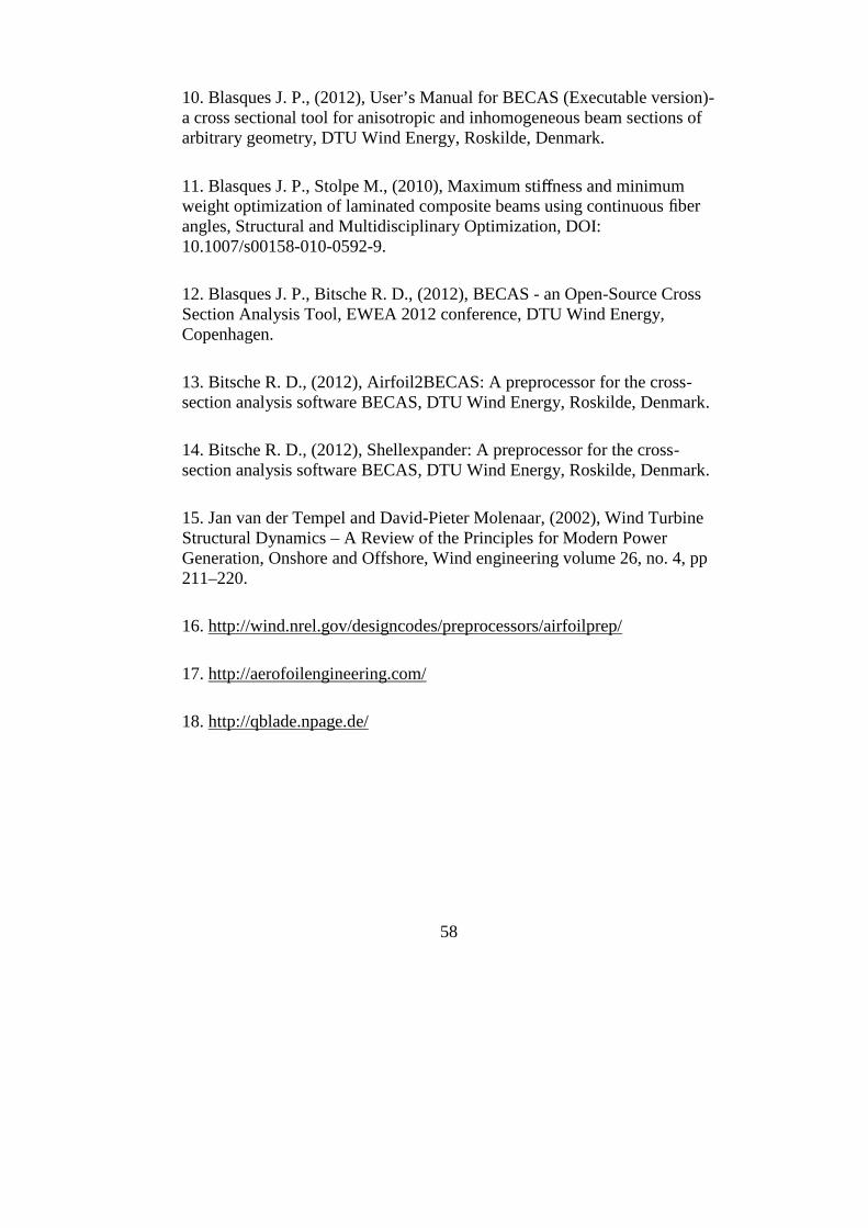
The animation of the fully modelled Nimbus 5.2 is shown in the Figure 4.8.The natural frequency analysis is done by the simulation in HAWC2. Themode shapes and Eigen frequencies of the whole turbine structure havebeen calculated. The natural frequencies of each main body are alsocalculated. The first 5 natural frequencies of the whole turbine structure areshown in the table below. The natural frequencies are evaluated in 2 cases.

51

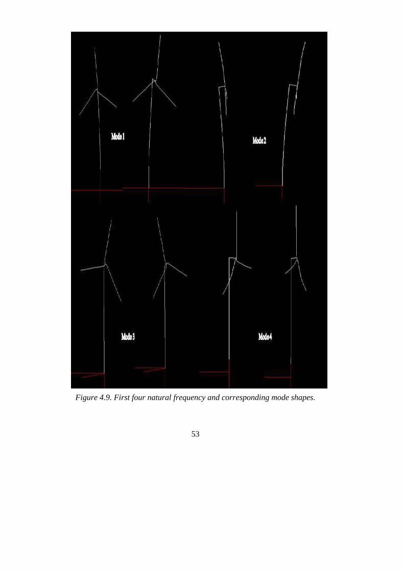
4.1.1 Case 1. Fully rigid structure

In this case both the yaw bearings and the main shaft bearings in the windturbine structure are deactivated and the turbine is considered as a singlerigid structure. The natural frequency of vibration and corresponding modeshapes for the specified case are shown below. The .htc file code for thesame has been attached in the Appendix A.

Figure 4.8. HAWC2 representation of Nimbus 1.6 KW.

4.1.2 Case 2. Main bearing activated

In this case the bearing shaft is being activated and the frequency analysis isconducted again. The natural frequency of vibration slightly varies in thiscase. The results are shown in table 4.1 shown below

52

Table 4.1. Natural frequency of the structure

Mode Shapes Case 1. Fixed Shaft

Natural Frequency(Hz)

Case2. Bearing Shaft

Natural Frequency(Hz)

1st tower transverse 1.29174E+00 1.29220E+00

1st tower longitudinal 1.31710E+00 1.31723E+00

1st rotor torsion 2.02101E+00 2.02314E+00

1st asymmetric rotorflap/yaw

2.87379E+00 2.87908E+00

1st asymmetric rotorflap

2.99097E+00 2.99822E+00

1st rotor edge 1 4.74724E+00 4.74725E+00

1st rotor edge 2 5.96903E+00 5.97965E+00

53

Figure 4.9. First four natural frequency and corresponding mode shapes.

54

5 Conclusions

The estimation of natural frequency of the system has been done withsuitable linearisation of the whole system. The damping of the system hasnot been tuned to obtain the the damped frequency of the system. It isimportant to find the damped frequency and correspondonding mode shapesbased on the need of the requirements of the study. The damping in the realstructure can be far more different from the damping in the real case whichdepends upon the material , the material plane orientation, the frictionacting between the layers etc. The more precise estimation of dampingrequires experience with usage of the material and suitable experimentalcase. Another way of addressing this problem is to estimate the requireddamping and give the design engineers the amount of damping correspondsto the particular mode shapes. Designers can achieve this value by tunedmass damper by distributing the mass accordingly or to choose fixationpoints which dissipate enough energy to insert sufficient damping.

Its very important to understand that how linearisation has been done in thedesign process. As we can see that the rotor blades are placed such that thefirst rotor blade is kept exactly vertical and the other two rotor blades at anangle of 120 degrees apart. This can be visualised in a clock as 0, 4 and 8O’clock configurations. The mass of the rotor blades are distributed in thismanner will be different when the rotor blades starts rotating. To taken thisinto account the eigen frequencies of the HAWT has been analysed bykeeping the two rotor blades up and the third one, when we look in a clockits like, 2 O’clock, 6 O’clock and 10 O’clock.

This configuration is then analysed and it is found that the naturalfrequencies remains the same. The changes of the natural frequency inbetween these two configurations is given below. It has been found that thenatural frequency of the structure has no change with respect to thedifferent configurations depending upon how the rotor mass is beingdistributed at any instant of time. This can been interpreted from the factthat the mass of the rotor blades are very less compared to the mass of thebig structural components like the tower or the hub mass.

55

Figure 5.1. (a) 2 O’clock, 6 O’clock and 10 O’clock configuration(b)3O’clock, 7 O’clock and 11 O’clock configuratin

Modeshapes

Naturalfrequency

FN (Hz)Default

Naturalfrequency FN

(Hz)Configuration 2

Naturalfrequency FN

(Hz)Configuration 3

Mode nr: 1 1.29174E+00 1.29174E+00 1.29174E+00

Mode nr: 2 1.31710E+00 1.31710E+00 1.31710E+00

Mode nr: 3 2.02101E+00 2.02101E+00 2.02101E+00

Mode nr: 4 2.87379E+00 2.87379E+00 2.87379E+00

Mode nr: 5 2.99097E+00 2.99097E+00 2.99097E+00

56

6 Future works

The structural and aerodynamic modelling of the whole wind turbine iscompleted. The wind is modelled inside the turbulence box and the windturbine is being positioned inside the turbulence box and has beensimulated. It can be seen that at some instant of the simulation thesimulation colapses due to the hitting of the rotor blades into the tower.This is due to the the lack of time in estimating the correct damping in thestructure. As discussed before it is really hard to estimate the real dampingin the structure due to its complex behaviour in the real structures comparedto theoretical model. The major future works required are

Estimation of real damping in the structures and implementing inthe model.

Tuning of damping for 3% logarithimic decrement between modeshapes as per RISOE DTU HAWC2 program developers method.

Implementing Enbreeze pitch control mechanism DLL and connectit to the HAWC2 interface

IEC simulations for certifications procedures.

Modelling of Soil and foundation.

57

7 References

1. Friedmann P P, (1976), Aeroelastic modeling of large wind turbines,

Journal of the American Helicopter Society, 21(4).

2. Larsen T J, Madsen H A, Hansen A M, Thomsen K, (2005),Investigations of stability effects of an offshore wind turbine using the newaeroelastic code HAWC2, http://wind.nrel.gov/public/SeaCon/Proceedings/Copenhagen.Offshore.Wind.2005/documents/papers/Poster/T.J.Larsen_Investigationofstabilityeffectsofano.pdf

3. Jonkman, J. M., and Buhl, M. L., Jr., (2004), FAST User's Guide,”NREL/EL-500-29798, Golden, CO: National Renewable EnergyLaboratory.

4. Bossanyi E A, (1996), GH Bladed Theory and User Manuals. England:

Garrad Hassan and Partners Limited.

5. Hansen A C, Laino D J, (1998), YawDyn and AeroDyn for ADAMS,http://wind.nrel.gov/designcodes/papers/ydguide11.Pdf.

6. Torben J. Larsen, Anders M. Hansen, (2012), How to HAWC2, theuser’s manual. Tech. Rep. Risø-R-1597(ver.4-3) (EN), DTU Wind Energy,Roskilde, Denmark.

7. A. Ahlstrom, (2002) Simulating Dynamical Behaviour of Wind PowerStructures. Technical Report:11, Royal Institute of Technology,Department of Mechanics, Licentiate Thesis, Stockholm, Sweden.

8. Torben J. Larsen, (2013), Introduction to HAWC2, Presentation onHAWC2, DTU Wind Energy, Roskilde, Denmark.

9. www.hawc2.dk.

58

10. Blasques J. P., (2012), User’s Manual for BECAS (Executable version)-a cross sectional tool for anisotropic and inhomogeneous beam sections ofarbitrary geometry, DTU Wind Energy, Roskilde, Denmark.

11. Blasques J. P., Stolpe M., (2010), Maximum stiffness and minimumweight optimization of laminated composite beams using continuous fiberangles, Structural and Multidisciplinary Optimization, DOI:10.1007/s00158-010-0592-9.

12. Blasques J. P., Bitsche R. D., (2012), BECAS - an Open-Source CrossSection Analysis Tool, EWEA 2012 conference, DTU Wind Energy,Copenhagen.

13. Bitsche R. D., (2012), Airfoil2BECAS: A preprocessor for the cross-section analysis software BECAS, DTU Wind Energy, Roskilde, Denmark.

14. Bitsche R. D., (2012), Shellexpander: A preprocessor for the cross-section analysis software BECAS, DTU Wind Energy, Roskilde, Denmark.

15. Jan van der Tempel and David-Pieter Molenaar, (2002), Wind TurbineStructural Dynamics – A Review of the Principles for Modern PowerGeneration, Onshore and Offshore, Wind engineering volume 26, no. 4, pp211–220.

16. http://wind.nrel.gov/designcodes/preprocessors/airfoilprep/

17. http://aerofoilengineering.com/

18. http://qblade.npage.de/

59

A. HAWC2 structural input file, fixedrotor

begin Simulation;

time_stop 0.1;

solvertype 1 ; (newmark)

on_no_convergence continue ;

convergence_limits 1E3 1.0 0.7 ;

logfile ./logfiles/structure_enbreeze.log ;

begin newmark;

deltat 0.02;

end newmark;

end simulation;

;

begin new_htc_structure;

beam_output_file_name ./logfiles/structure_beam_enbreeze.dat; Optional - Calculated beamproperties of the bodies are written to file

body_output_file_name ./logfiles/structure_body_enbreeze.dat; Optional - Body initial position andorientation are written to file

body_eigenanalysis_file_name ./eigenfrq/structure_body_eigen_enbreeze.dat;

structure_eigenanalysis_file_name ./eigenfrq/structure_strc_eigen_enbreeze.dat;

;----------------------------------------------------------------------------------------------------------------------------------------------------------------

begin main_body; tower 87m

name tower ;

type timoschenko ;

nbodies 1 ;

node_distribution c2_def ;

damping_posdef 8.142E-04 8.14E-04 4.0E-03 4.3E-04 4.3E-04 4.3E-03 ; Mx My Mz Kx Ky Kz , M´s raisesoverall level, K´s raises high freguency level

begin timoschenko_input;

filename ./data/NREL_5MW_st_enbreeze.txt ;

set 1 2 ;

end timoschenko_input;

begin c2_def; Definition of centerline (main_body coordinates)

nsec 8;

60

sec 1 0.0 0.0 0.0 0.0 ; x,y,z,twist

sec 2 0.0 0.0 -1.0 0.0 ;

sec 3 0.0 0.0 -2.0 0.0 ;

sec 4 0.0 0.0 -3.0 0.0 ;

sec 5 0.0 0.0 -4.0 0.0 ;

sec 6 0.0 0.0 -5.0 0.0 ;

sec 7 0.0 0.0 -5.5 0.0 ;

sec 8 0.0 0.0 -6.0 0.0 ;

end c2_def ;

end main_body;

;

begin main_body;

name towertop ;

type timoschenko ;

nbodies 1 ;


; damping_posdef 9.025E-06 9.025E-06 8.0E-05 8.3E-06 8.3E-06 8.5E-05 ;

damping 2.50E-04 1.40E-04 2.00E-03 3.00E-05 3.00E-05 2.00E-04 ;

concentrated_mass 2 0.0 0.0 0.0 242.3 34.50 32.64 29.06



set 2 2 ;



nsec 2;

sec 1 0.0 0.0 0.0 0.0 ; x,y,z,twist

sec 2 0.0 0.0 -0.2 0.0 ;

end c2_def ;

end main_body;

;

begin main_body;

name shaft ;

type timoschenko ;

nbodies 1 ;


; damping_posdef 7.00E-3 7.00E-03 7.00E-02 3.48E-04 3.48E-04 1.156E-03 ;

61

damping_posdef 7.00E-3 7.00E-03 7.00E-02 6.5E-04 6.5E-04 1.84E-02 ;

concentrated_mass 1 0.0 0.0 0.0 0.0 0.0 0.0 0.066 ;generator equivalent slow shaft

concentrated_mass 5 0.0 0.0 0.0 90.8 0.0 0.0 25.09 ; hub mass and inertia;



set 3 2 ;



nsec 5;

sec 1 0.0 0.0 0.0 0.0 ; Tower top x,y,z,twist

sec 2 0.0 0.0 0.15 0.0 ;

sec 3 0.0 0.0 0.25 0.0 ;

sec 4 0.0 0.0 0.35 0.0 ; Main bearing

sec 5 0.0 0.0 0.50 0.0 ; Rotor centre

end c2_def ;

end main_body;

;

begin main_body;

name hub1 ;

type timoschenko ;

nbodies 1 ;


damping_posdef 2.00E-05 2.00E-05 2.00E-04 3.00E-06 3.00E-06 2.00E-05;



set 4 2 ;



nsec 2;

sec 1 0.0 0.0 0.0 0.0 ; x,y,z,twist

sec 2 -0.1 0.0 0.141 0.0 ;

end c2_def ;

end main_body;

;

begin main_body;

name hub2 ;

62

copy_main_body hub1;

end main_body;

;

begin main_body;

name hub3 ;

copy_main_body hub1 ;

end main_body;

;

begin main_body;

name blade1 ;

type timoschenko ;

nbodies 1 ;

node_distribution c2_def;

; damping_posdef 1.16e-4 5.75e-5 6.1e-6 6.5e-4 5.1e-4 6.4e-4 ;

damping_posdef 3.1E-03 2.1E-03 3.6E-05 1.45E-03 2.3E-03 4.5E-05 ;

begin timoschenko_input ;


set 5 2 ; set subset



nsec 7 ;

sec 1 0.0000 0.0000 0.000 0.000 ;x.y.z. twist

sec 2 0.0000 0.0000 0.700 -0.000;

sec 3 0.13086 0.001 1.000 -8.56449;

sec 4 0.09687 0.008 1.300 -5.40606;

sec 5 0.08149 0.011 1.600 -3.33675;

sec 6 0.07216 0.012 2.050 -1.56943;

sec 7 0.03336 0.006 2.500 0.00000;

end c2_def ;

end main_body;

;

begin main_body;

name blade2 ;

copy_main_body blade1;

end main_body;

;

63

begin main_body;

name blade3 ;

copy_main_body blade1 ;

end main_body;

;----------------------------------------------------------------------------------------------------------------------------------------------------------------

begin orientation;

;

begin base;

body tower;

inipos 0.0 0.0 0.0 ; initial position of node 1

body_eulerang 0.0 0.0 0.0;

end base;

;

begin relative;

body1 tower last;

body2 towertop 1;

body2_eulerang 0.0 0.0 0.0;

end relative;

;

begin relative;

body1 towertop last;

body2 shaft 1;


body2_eulerang 0.0 0.0 0.0; 0 deg tilt angle

body2_ini_rotvec_d1 0.0 0.0 -1.0 0.2 ; body initial rotation velocity x.y.z.angle velocity[rad/s] (body 2coordinates)

; body2_ini_rotvec_d1 0.0 0.0 -1.0 0.9424 ; body initial rotation velocity x.y.z.angle velocity[rad/s] (body 2coordinates)

end relative;

;

begin relative;

body1 shaft last;

body2 hub1 1;

body2_eulerang -90.0 0.0 0.0;


body2_eulerang 0.0 0.0 0.0; 0deg cone angle

end relative;

64

;

begin relative;

body1 shaft last;

body2 hub2 1;


body2_eulerang 0.0 -60.0 0.0;


end relative;

;

begin relative;

body1 shaft last;

body2 hub3 1;




end relative;

;

begin relative;

body1 hub1 last;

body2 blade1 1;

body2_eulerang 0.0 0.0 0;

end relative;

;

begin relative;

body1 hub2 last;

body2 blade2 1;


end relative;

;

begin relative;

body1 hub3 last;

body2 blade3 1;


end relative;

;

end orientation;

65

begin constraint;

;

begin fix0; fixed to ground in translation and rotation of node 1

body tower;

end fix0;

;

begin fix1;

body1 tower last ;

body2 towertop 1;

end fix1;

; ;

; begin bearing1; free bearing

; name shaft_rot;

; body1 towertop last;

; body2 shaft 1;

; bearing_vector 2 0.0 0.0 -1.0; x=coo (0=global.1=body1.2=body2) vector in body2 coordinates wherethe free rotation is present

; end bearing1;

; ;

;

; begin bearing3; fixed speed bearing

; name shaft_rot ;

; body1 tower last;

; body2 shaft 1;

; bearing_vector 2 0.0 0.0 -1.0; x=coo (0=global,1=body1,2=body2) vector in body2 coordinates wherethe free rotation is present

; omegas 0.93245 ;

; end bearing3;

;

begin fix1;

body1 towertop last ;

body2 shaft 1;

end fix1;

;

begin fix1;

body1 shaft last ;

body2 hub1 1;

66

end fix1;

;

begin fix1;

body1 shaft last ;

body2 hub2 1;

end fix1;

;

begin fix1;

body1 shaft last ;

body2 hub3 1;

end fix1;

;

begin bearing2;

name pitch1;

body1 hub1 last;

body2 blade1 1;

bearing_vector 2 0.0 0.0 -1.0;

end bearing2;

;

begin bearing2;

name pitch2;

body1 hub2 last;

body2 blade2 1;


end bearing2;

;

begin bearing2;

name pitch3;

body1 hub3 last;

body2 blade3 1;


end bearing2;

end constraint;

;

end new_htc_structure;

exit;

67

B. Parameter File airfoil2BECAS, rotorblade section 3.

# This is a sample parameter filed to be used with airfoil2becas.py

# #################################################################

# Name of the directory for storing results

# #################################################################

outputdir = "testairfoil_BECAS_input_section3"

# The directory will be generated in the current working directory.

# If the directory already exists, it is deleted.

# Name of the file containing the x-y-coordinates of the airfoil

# #################################################################

airfoilfilename = "testairfoil_section3.dat"

# The number of elements used to discretize the shell thickness.

# The minimum value is the largest number of layers of different material

# anywhere in the airfoil.

element_layers = 10

# Shear Webs

# #################################################################

# Shear webs are defined as straight lines connecting two airfoil

# nodes. Any number of shear webs can be defined. The syntax is:

# shear_webs = [ [web1_from_node, web1_to_node],

# [web2_from_node, web2_to_node] ]

# If no shear webs should be generated, an empty list must be defined:

# shear_webs = []

# The corresponding regions for layup assignment are:

# REGION09, REGION10, ...

shear_webs = [ [25, 73],

[30, 68],

[40, 60] ]

68

# Layup defintion

# #################################################################

# The layup is defined as a list of lists using the following syntax:

# [ [layerthickness1, int. points1, materialname1, orientationangle1, plyname1],

# [layerthickness2, int. points2, materialname2, orientationangle2, plyname2],

# [layerthickness3, int. points3, materialname3, orientationangle3, plyname3] ]

# The first layer is the outer most layer.

# The second item ("int. points") and the fifth item ("plyname") are not

# relevant. The are kept for compatibility with the ABAQUS input syntax.

layup_of_elset = {} # initialize empty dictionary

layup_of_elset['REGION01'] = [ [0.003, 3, 'PE', 0.0, 'Ply01'] ]

layup_of_elset['REGION02'] = layup_of_elset['REGION01']

layup_of_elset['REGION03'] = [ [0.003, 3, 'PE', 0.0, 'Ply05'] ]






layup_of_elset['REGION09'] = [ [0.00000001, 3, 'PE', 0.0, 'Ply09'],

[0.00000001, 3, 'PE', 0.0, 'Ply10'],

[0.00000001, 3, 'PE', 0.0, 'Ply11'] ]



# Number of elements in each shear web

# #################################################################

# The "height" of the elements representing the web must be larger

# than the thickness of the cap.

# Check the mesh at the intersection of the shear web and the cap.

# A list of integer numbers (one for each shear web) must be given.

# e.g. number_of_web_elements = [10, 12, 8]

# If no shear webs should be generated, an empty list must be defined:

# number_of_web_elements = []

number_of_web_elements = [5, 5, 3]

69

# Reverse normals

# Should the normals be reversed? That is, should the material

# layers be added in the other direction? Default: False

# WARNING: Only set this to True if you exactely know what you

# are doing!

reverse_normals = False

# Material Parameters

# #################################################################

# The definition of an orthotropic material requires 9 elastic constants:

# E1, E2, E3, nu12, nu13, nu23, G12, G13, G23.

# In the case of an isotropic material use:

# E1 = E2 = E3 = E

# nu12 = nu13 = nu23 = nu

# G12 = G13 = G23 = E/(2*(1+nu))

# 'rho' is the mass density

material_properties = {} # initialize empty dictionary

material_properties['PE'] = {

'E1': 900E6,

'E2': 900E6,

'E3': 900E6,

'nu12': 0.46,

'nu13': 0.46,

'nu23': 0.46,

'G12': 308E+6,

'G13': 308E+6,

'G23': 308E+6,

'rho': 958 }

70

C. Wind Turbulence Box, HAWC2

begin wind ;

density 1.225 ; to be checked

wsp 7 ;

tint 0.2 ;

horizontal_input 1 ; 0=false, 1=true

windfield_rotations -0.0 0.0 0.0 ; yaw, tilt, rotation

center_pos0 0.0 0.0 -6.2 ;

shear_format 3 0.2 ;0=none,1=constant,2=log,3=power,4=linear

turb_format 1 ; 0=none, 1=mann,2=flex

tower_shadow_method 1 ; 0=none, 1=potential flow, 2=jet

; scale_time_start 0 ;

; wind_ramp_factor 0.0 [t0] [wsp factor] 1.0 ;

; [gust] iec_gust [gust_type] [gust_A] [gust_phi0] [gust_t0] [gust_T] ;

;

begin mann;

create_turb_parameters 29.4 1.0 3.7 1 1.0 ; L, alfaeps,gamma,seed, highfrq compensation

filename_u ./turb/u.bin ;

filename_v ./turb/v.bin ;

filename_w ./turb/w.bin ;

box_dim_u 1024 0.410155625 ;

box_dim_v 32 0.5;

box_dim_w 32 0.5;

std_scaling 1.0 0.7 0.5 ;

end mann;

;

begin tower_shadow_potential;

tower_offset 0.0 ;

nsec 2;

radius 0.0 0.076 ;

radius -6.0 0.076 ;

end tower_shadow_potential;

end wind;

aeroelastic simulation of small wind t urbine using...

Documents