affine relationships among variables of a program
TRANSCRIPT
Acta Informatica 6, 133--151 (1976) �9 by Springer-Vedag t976
Affine Relationships Among Variables of a Program*
Michael Kar r
Received May 8, 1974
Summary. Several optimizations of programs can be performed when in certain regions of a program equality relationships hold between a linear combination of the variables of the program and a constant. This paper presents a practical approach to detecting these relationships by considering the problem from the viewpoint of linear algebra. Key to the practicality of this approach is an algorithm for the calculation of the " s u m " of linear subspaces.
1. Problems in Need of a Solution
A class of problems in the optimization of programs centers around the need to relate affine combinations of program variables (linear combinations plus a constant). In the development of the IVTRAN compiler for the ILLIAC IV, for instance, much effort is spent in the "parallelizing" of nested DO loops. One requirement is tha t the upper and lower limits for a given loop be expressible as a function of the index variables of containing DO loops. In practice, these rela- tionships are almost invariably affine (linear plus a constant) in the other index combinations. Because of FORTRAN syntax restrictions, expressions cannot appear as DO loop limits; this directly gives us the problem of the determination of whether, at a given point in a program, a variable is some affine combination of other variables.
Naturally, the above problem could be solved most of the t ime by an ad hoc analyzer built especially for the purpose of recognizing the common situations. However, a seemingly unrelated problem m a y be expressed in the same terms. A common optimization known as "reduction in operator s t rength" occurs in source code, because wise programmers often know that their particular compiler does not do the transformation for them. This optimization converts a sequence of "expensive" operations--multiplications of a loop index by a constant - - in to a series of " cheape r " operat ions--addit ions of the constant to a "co-index". On serial machines, this transformation is indeed an optimization; however, on a parallel machine, it is preferable to do ** multiplications at the same t ime than to perform n successive additions. Thus, the transformation must be reversed. This problem m a y at first seem difficult, and the usual suggestion is to find a "heur is t ic" which will solve it most of the time. But observe tha t such a trans- formation always stems from some linear expression involving a loop index, and
*~ This research was supported by the Advanced Research Projects Agency of the Department of Defense and was monitored by U. S. Army Research Office--Durham under Contract No. DAHC04-70-C-O023.
134 M. Karr
hence always introduces some affine relationship between the variable to be incremented by the series of additions (the co-index) and the loop index. Again, a knowledge of affine relationships among variables would enable us to solve a problem.
The above problems arise from the standpoint of optimization by paraUelizing. Even in more classical optimization problems, a knowledge of affine relationships is applicable. For instance, constant propagation may be viewed as the recognition of such facts as I----t at some point in a program (i.e., that statement is true every time flow of control is at the point). Such a relationship is a special case of an affine relationship among variables. This suggests that we could do a more general form of constant recognition, that is, we could recognize when linear forms are constants (even though their constituents might not be). Further, if in the detection of affine relationships, we make full use of the content of decision nodes, the constant detection machinery will thereby have a natural way of using the content of decision nodes in the detection of constants. For example, if the flow- block beginning at t00 is uniquely accessible from the statement IF (I .EQ. 0) GO TO 100, then all occurrences of I in that flowblock may be replaced by 0.
Another application is in the recognition of common subexpressions which are not identical formally, but are the same because of relationships among variables. If these relationships are affine, then we can detect otherwise overlooked common subexpressions.
The existence of the common thread running through the above problems suggests at least making an at tempt to develop a general technique for analyzing affine relationships among program variables. This paper shows that a unified approach to these problems is indeed feasible.
2. Representation of Affine Relationships
2.1 Choices Involved
Suppose that the scalar variables of a program are denoted by ~; let V----- (V 1 . . . . . V~). Each variable has values in a field F, which in practice may be the rationals or the reals. From a mathematical point of view, to say that a given affine relationship holds among the values of the variables at a given point in the program is to say that for any execution of the program, when the flow of control reaches the given point, then the vector of values V always lies in some fixed affine subspace 1 of F ~. As the affine relations become more numerous, the subspace has smaller and smaller dimension. If the subspace has dimension O, then V is a con- stant, with each V~ taking on the value of the i th coordinate of the point. If the relations are contradictory, then the subspace is the null set, and may be thought of as having dimension --co. At the other end, if there are no affine relationships, then the corresponding subspace is the entire space F ' , and has dimension n.
If we wish to make use of affine relationships, we must have a scheme for the finite representation of these (possibly infinite) spaces. There are basically two
t Intuitively, an affine subspace is a point, line, plane, etc., not necessarily passing through the origin. See Ill, Chapter XII for details.
Affine Relationships Among Variables of a Program t 3 5
methods for representing affine subspaces. One way is to represent a subspace by a basis of its linear component, plus an offset vector. A second way is to represent the space as the kernel of an affine transformation ~ from F ~ to F • for appropriate m. Luckily: there is no real debate over which method to choose, when we consider the fact tha t in most programs, the number of affine relationships will be small--i .e. , the subspace will be large. The first method of representation requires as many basis elements as the dimension of the subspace.
In the second method, the representation is inverse!y related to the size of the space. Suppose tha t there are m independent affine relationships. These can be represented by a m • n matr ix A, and a vector e of length m, where the map is:
(A, e ) : F" - , F ~
(2.t) V ~ A V - - e
ker (A, e) ~ ( V ] A V = e , i.e., AV--e----0}.
The kernel of this map has dimension n - - m. Thus, if there are no relations at all, the matr ix and vector are "empty"; the more relations there are, the more rows the matr ix A must have, but then that much more useful information has been extracted from the program. There is one affine subspace which cannot be re- presented by a matr ix-vector pair, namely the null set; it may be represented by a reserved symbol, say ~.
2.2 Canonical Form
There is a further issue in the representation of affine relationships. Several different matr ix-vector pairs m a y represent essentially the same set of relation- ships; viewed as maps as in (2A), their kernel is the same. We shall see tha t it is important tha t identical predicates have identical matr ix-vector pairs representing them. Elementary linear algebra fortunately provides us with a " canonical fo rm" for this problem. The proper ty we require of this form is:
(2.2) Let (Ai, ei) , i = t , 2 be two matr ix-vector pairs in canonical form. Then:
ker (A v c l ) = k e r (A v c2)r 1 = A 2 and e x =c~.
The particular canonical form which is appropriate for our purposes is" normalized reduced row-echelon form". Our reference on this is [2], to which the reader is referred for proofs; we shall present t he definitions, because they are useful later in this paper.
def (2.3) The matr ix A is in row-echelon form r
(a) Every row of A has at least one non-zero entry.
(b) For any row i o, let J0 be the first column with a non-zero entry of the row. Then for all i > i o,/" _~ is, A~j = 0.
Row operations, namely those which mult iply a row by a non-zero scalar, or which add a row to another row, or which permute two rows, m a y be used to
2 An affine transformation maps affine subspaces to affine subspaces. Its kernel is the set of elements mapped to the origin, and is itself an affine subspace.
t 36 M. Karr
transform any matrix A so that it satisfies (2.3 b). When performing row opera- tions on (A, e~, e is t reated as the n + t st column; such operations leave the kernel of (A, e ) unchanged. The kernel is also unchanged if an entire row of zeros is deleted from (A, e~. If the i m row of A is zero, but c i ~= 0, then the kernel of (A, e ) is null, and the space would be represented by ~. Hence, we can transform a pair (A, e~ until the matr ix is in row-echelon form, or the kernel is discovered to be null. (Deletions of zero rows may result in an "empty" matrix-vector pair, whose kernel is all of F~-- this is different from ~, which is none o f /~ , )
(2.4) Let A be in row-echelon form. Then the column index of the first non-zero entry of row i is denoted Pi. The columns whose indices are {Pi}~=l are called the dependent columns. The rest are the independent columns.
Notice that if i 1 > is, then Pil > Q~,. The motivat ion for the names of column groupings comes from the theory of the solution of simultaneous linear equations.
def (2.5) The matr ix A is in reduced row-echelon form r
(a) A is in row-echelon form, and
(b) If i< io then A~p~, = 0 .
Any matrix-vector pair satisfying (2.3) may be made to satisfy (2.5) simply by applying appropriate row operations. At this stage, there is no possibility that the kernel m a y be discovered to be null.
(2.6) The matr ix A is said to be normalized ~=~ the first non-zero element o f each row of A is t.
Clearly, any matr ix m a y be normalized by the row operations of multiplications by suitable non-zero elements of F. In practice, it may be more convenient to use other normalization conditions; the above is the most convenient for purposes of this paper.
3. Deriving Valid Relationships
Following Floyd [3], we shall a t tach our particular form of assertions to the arcs of a program graph: on arc x, the s ta tement of affine relationships will be represented by (A,, e,) . The subject of this paper will not be the algorithm for "push ing" assertions around the program graph. Wegbreit [4] points out that this problem can be considered independently of the nature of the particular assertions which one is pushing. In this paper, we shall follow the basic outlines of [4]. The termination and correctness of proofs of that paper apply to the specific case analyzed here.
For purposes of exposition, we shall view the program graph as having three types of nodes: assignment, decision, and merge. No computation is contained in merge nodes, which have only one exit arc, as do assignment nodes. The computa- tion of the right-hand side of an assignment s tatement and of the expression in a decision node are assumed not to affect the values of any variables. Thus, all side-effect phenomena must be modeled as assignment statements,
Affine Relationships Among Variables of a Program t 3 7
The basic idea of Wegbreit 's algorithm as applied to affine relationships is to start with some (A, e ) on the entry arc to the program, which represents what is known about the variables at the start of execution. This is typically the empty matrix-vector pair (representing that nothing is known), though if the variables are initialized to 0, then the pair ( I , 0) is appropriate, where I is the identity matrix. All of the other arcs are initialized to # .
For each of the three different types of nodes, we shall describe a transforma- tion which specifies affine space(s) for the output arc.(s) of the node in terms of t) the affine space(s) on the input arc(s) to the node, and 2) where relevant, the content of the node. The transformations all have the property that if the input assertions are all true (for every execution of the program which passes through the arc) then the output assertions are true. The algorithm of E4] consists of applying these transformations until all the assertions are "stabi l ized" --i.e., the application of a transformation at any node results in no change in the assertions on the output arcs.
The proof in [41 that this algorithm terminates is, for affine assertions, due to t h e " ascending chain condition" which holds for finite-dimensional affine spaces-- namely, any properly ascending chain of sub-spaces:
is finite. This is obvious, for each of the subspaces U i must have a dimension of at least one greater than Ui- v Since the dimension of any Ui is limited by n, such a sequence cannot continue indefinitely.
The rest of this paper deals with the transformations at each of the three different kinds of nodes, and with the details of the calculations involved in carrying out these transformations. In the examples, we shall use the algorithm described loosely above, in more detail in [4].
4. Node Functions
4.1 Decision Nodes
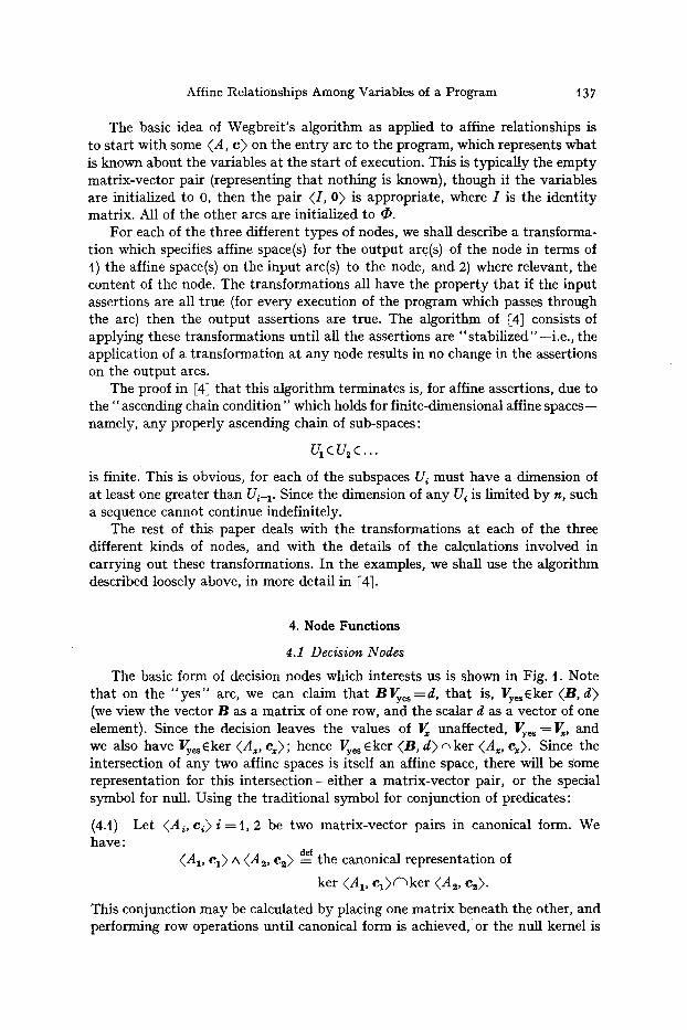
The basic form of decision nodes which interests us is shown in Fig. t . Note that on the " y e s " arc, we can claim that BVyes=d, that is, Vy~Eker (B, d) (we view the vector B as a matrix of one row, and the scalar d as a vector of one element). Since the decision leaves the values of V~ unaffected, Vy~ = V~, and we also have VyesEker (Az, ex); hence Vyes Eker (B, d) ~ ker (Ax, ex). Since the intersection of any two affine spaces is itself an affine space, there will be some representation for this intersection--either a matrix-vector pair, or the special symbol for null. Using the traditional symbol for conjunction of predicates:
(4.t) Let (A o e~) i = 1, 2 be two matrix-vector pairs in canonical form. We have:
(A 1, e l ) ^ (A~, e~) de f the canonical representation of
ker (Ax, el)(-hker (A~, e~).
This conjunction may be calculated by placing one matrix beneath the other, and performing row operations until canonical form is achieved, o r the null kernel is
138 M. Karr
oo[ Fig. I
yes
detected. This gives us the appropriate predicate to be placed on the "yes" arc:
(A,, e,) ^ (B, d).
The predicate for the "no" arc cannot directly incorporate the affine non- equality. If (A,, e,) ^ (B, d) = (A,, e,), then ker (B, d) _(ker (A,, e,) and flow always leaves through the " y e s " arc; in this case �9 is a valid predicate for Ano. Otherwise, we cannot add any information to (A,, e,), and must be content with that predicate itself on the "no" arc. In summary, the predicate for the "no" arc is:
if (A~, e~) is the predicate for the " y e s " arc;
(A,, e,) otherwise.
In ESl, a general s tudy is made of how best to handle decision nodes which are not of the simple form of Fig. t. For purposes of this paper, we may handle such nodes merely by placing (A~, e~) on each of the output arcs. This is certainly valid, but it may not be as much information as could be gathered.
4.2 Assignment Nodes
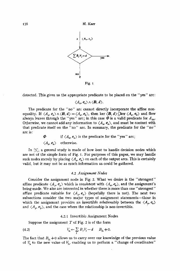
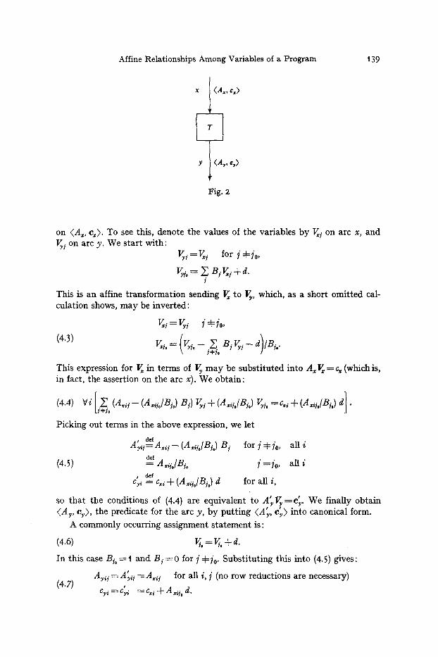
Consider the assignment node in Fig. 2. What we desire is the "strongest" affine predicate (Ay, ey) which is consistent with (A,, e,), and the assignment's being made. We also are interested in whether there is more than one "strongest" affine predicate suitable for (Ay, ey) (hopefully there is not). The next two subsections consider the two major types of assignment statements--those in which the assignment provides an invertible relationship between the (Ax, e,) and (Ay, ey), and the case where the relationship is non-invertible.
4.2.t Invertible Assignment Nodes
Suppose the assignment T of Fig. 2 is of the form
(4.2) ~.<- Z B j ~ + d Bi. 4:0. i
The fact that Bio 4:0 allows us to carry over our knowledge of the previous value of ~0 to the new value of ~0, enabling us to perform a "change of coordinates"
Affine Relationships Among Variables of a Program
~ , rx)
139
y <A,, *,>
Fig. 2
on (A,,, e~). To see this, denote the values of the variables by V~ i on arc x, and Vyj on arc y. We start with:
~; =V~ for i * i o ,
5i. = ~ Bi V~i + d. i
This is an affine transformation sending ~ to Vy, which, as a short omitted cal- culation shows, may be inverted:
v, i = v~; i * io ,
(4.3) V, = (V,q _ j~. B, V~i_ d)/Bi..
This expression for ~ in terms of ~ may be substituted into A~ V x = c~ (which is, in fact, the assertion on the arc x). We obtain:
(4.4) Vi[ E ( A , , j - (A,,io/Bio) Bi) Vy i + (A,,io/Bio) Vyi. =c,,, + (A,ai~ d] . ki*io ]
Picking out terms in the above expression, we let
t d e f
A#i=A,q - - (A~ io /B i . ) B i for i4 : io , a l l i d e f
(4.5) = A,iio/Bio f =fo, all i t d e f
cy~ = c~i + (A~ii./Bj~ d for all i,
t t so that the conditions of (4.4) are equivalent to AyVy =ey. We finally obtain r t
(Ay, %), the predicate for the arc y, by putting (Ay, ey) into canonical form.
A commonly occurring assignment statement is:
(4.6) v,.~ = vj. + d.
In this case Bi~ and B i = 0 for i 4=/'o. Substituting this into (4.5) gives: t
Ayi i ~-A~ii ~-A,~ i for all i, i (no row reductions are necessary ) (4.7)
cy i ---c~ = c:i + A Xqo d.
t40 M. Karr
Furthermore, if d - -0 , we have ey-----e,, which is reassuring: if the assignment changes nothing, the affine space carries over unchanged.
4.2.2 Non-Invertible Assignment Nodes
If the assignment statement is not of the form of (4.1), then it appears that we cannot solve for V, in terms of Vy, and we have " los t " some information by the assignment to 4~ This loss has to do with the fact that old relationships involving 40 and other variables no longer hold true. If the 1'~ column of Ax is entirely zero, then (A x, e,> is independent of the value of V/o, and is thus valid for the arc y. Otherwise, we must remove the dependence of (Ax, e~) on ~ . The obvious way to do this is to remove the rows of A~ which have a non-zero entry in the i th column (and the corresponding elements of e,). A better way is to:
(4.8) Let i o be the last row in which the ~'o th entry is non-zero. Reduce rows 1, . . . , i o -- 1 by row i 0 to make the 1'~ entry zero (rows i o + t . . . . . m already have zeros as the ?'~ entry, by canonical form). Then, remove row i 0 and call the result <A~, cy>.
The reader may verify that the (Ay, ey) thus produced is in canonical form, and that its 1"~ column is zero. Nevertheless, the rule seems arbitrary, since it appears that the resulting space might be different if we had picked another row to reduce by, and then to eliminate; it might also depend upon column order (which affects canonical form). In fact, these fears are groundless, and (4.8) may be shown to be, in some sense, the unique " b e s t " that can be done under the circumstances. This analysis, which also shows an underlying connection between the invertible and non-invertible case, is unfortunately too lengthy and general for inclusion here; the reader is referred to [5].
Once we have weakened the predicate, if necessary, to delete information about 4~ we again examine the right-hand side of the assignment. If it is some non-affine function of the other program variables, then we may make no new statements of affine relationship. If, however, the statement is of the form:
(4.9) 4 < - ~ B j ~ +d . i.i~
then we may add to our list of other relationships the statement
, , I - -Bi if /4=/0 ~ B iVii=d where Bi----t t otherwise J" ?
Applying (4.t), the better definition for this case is: def
(4.10) (Ay, cy) = <B', d>A <A',, e',)
where (A',, c'x> is the matrix-vector pair obtained in (4.8).
4.3 Merge Nodes
I t is in this section that the most difficult problem is confronted. Consider Fig. 3. On each of the input arcs x, we have some affine space (A x, ex). What is
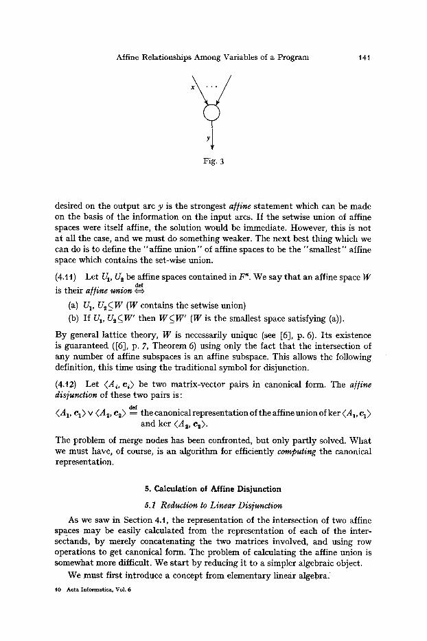
Affine Relationships Among Variables of a Program
Fig. 3
14t
desired on the output arc y is the strongest affine statement which can be made on the basis of the information on the input arcs. If the setwise union of affine spaces were itself affine, the solution would be immediate. However, this is not at all the case, and we must do something weaker. The next best thing which we can do is to define the "affine union" of affine spaces to be the "smallest" affine space which contains the set-wise union.
(4.t t) Let U1, U 2 be affine spaces contained i n /~ . We say that an affine space W def
is their a]fine union r
(a) U 1, U, ( W (W contains the setwise union)
(b) If U1, U2(_W" then W(_W' (W is the smallest space satisfying (a)).
By general lattice theory, W is necessarily unique (see [6], p. 6). Its existence is guaranteed ([6], p. 7, Theorem 6) using only the fact that the intersection of any number of affine subspaces is an affine subspace. This allows the following definition, this time using the traditional symbol for disjunction.
(4.t2) Let (Ai, e~) be two matrix-vector pairs in canonical form. The a]]ine disjunction of these two pairs is:
(A v ca) v (A ~, e2) de~ the canonical representation of the affine union of ker (Ax, e x) and ker (A2, e2).
The problem of merge nodes has been confronted, but only part ly solved. What we must have, of course, is an algorithm for efficiently computing the canonical representation.
S. Calculation of Affine Disjunction
5.1 Reduction to Linear Disjunction
As we saw in Section 4.t, the representation of the intersection of two affine spaces may be easily calculated from the representation of each of the inter- sectands, by merely concatenating the two matrices involved, and using row operations to get canonical form. The problem of calculating the affine union is somewhat more difficult. We start by reducing it to a simpler algebraic object.
We must first introduce a concept from elementary linear algebra.
10 Acta Informatica, Vol. 6
142 M. Karr
(5.t) A linear subspace of F" is an affine subspace which contains the origin. (This is hardly the traditional definition, but is convenient here.)
We may represent a linear subspace by a matrix, similarly to the way in which a matrix-vector pair represents an affine subspace.
(5.2) For an m X n matrix A, view
A: F~-~F m
V ~ A V .
ker A d,f {V]AV=O}.
Analogous to the situation in 2.2, there is a one-one correspondence between linear subspaces of F ~, and matrices in reduced row echelon form.
Observe that the affine union of two linear subspaces is again linear; this is traditionally called the sum of the two subspaces, and is denoted by + . The correspondence between linear subspaces and matrices in canonical form thus induces an operation on these matrices, analogous to (4.t2). We shall again use v to denote this operation; context will distinguish this "linear disjunction" from the "affine disjunction" which previously used the same symbol. The two opera- tions are in fact closely related. To see how, let
(5.3) (A, e) ae~ the m x (n + t) matrix formed from the m • n matrix A by adjoining the m-element vector e as the n + t st column.
Quite conveniently, linear sum in F s+t corresponds to affine union in F ' :
(5.4) Let A 1, A s be n-column matrices in canonical form, and e a, e 2 be vectors of the proper lengths. Let (A, c ) be the matrix-vector pair defined by (Ax, th) v (A 2, c2). Then
(A, c) ----- (A 1, cl) v (A s, cz).
In other words, the n + t-column matr ix produced by linear disjunction, and that produced by affine disjunction, are the same.
(A proof may be found in the Appendix.) This reduces the problem of affine dis- junction to that of linear disjunction, which we consider next.
5.2 Calculation o/ the Linear Disjunction
We shall give here an efficient algorithm, in terms of both time and space, for the calculation of the matrix which represents the union of two linear subspaces, given the two matrices which represent the subspaces whose union is to be taken.
We shall assume that the matrices A and B are given in canonical form, and we shall produce a matrix C, again in canonical form, which represents the union. The algorithm consists of n steps, where n is the number of columns. I t proceeds by modifying the original natrices A and B so that at the end of step s, the first s columns of the modified A and B are the same. At the end of n steps, both matrices
Affine Relationships Among Variables of a Program t43
are the same; the affine union of identical spaces is of course the space itself, and so we will have arrived at the desired result. The algorithm is started by:
(5.5) ACO) d~ ACoO ) d~ A ; BCo} de~ B~Ol d~ . . . . B; C I~ is the "ma t r ix with no rows or columns".
For any matrix D, [DI de~ the number of rows of D.
At the completion of step s, the following four conditions will hold
(5.6.t) ker A (~) + ker B I~l = ker A + ker B (sum of linear subspaces)
(5.6.2) A I'l = ( - ~ A{oSl) ; B (s} = (C~*)[ B~S)).
(Unlabelled submatrices of a parti t ion are assumed to be filled with zeros. A~ ~), B~ ~1 are defined to be submatrices of A {'~, B Is} respectively, consisting of of columns s + I . . . . . n.)
(5.6.3) A Cs), B Is} and C csl are all in canonical form
(5.6.4) C Is} is s columns wide. (We will also have 0 ~ [C(Sl[ _~ s, where the fact that it has no rows but s columns means that the first s columns of A {s) and B {s} are zero.)
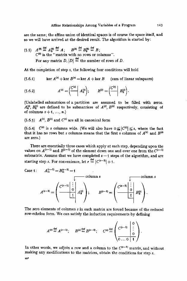
There are essentially three cases which apply at each step, depending upon the values on A Is-~} and B {s-l} of the element down one and over one from the C {s-l} submatrix. Assume that we have completed s - - l steps of the algorithm, and are
starting step s. For convenience, let r ~ [Cr + t.
Case I : Acs-1} R(s-1) = I
column s ~ column s
The zero elements of columns s in each matr ix are forced because of the reduced row-echelon form. We can satisfy the induction requirements by defining
o
\ o . . . o
In other words, we adjoin a row and a column to the C (s-ll matrix, and without making any modifications to the matrices, obtain the conditions for step s.
t 0 "
t44 M. Karr
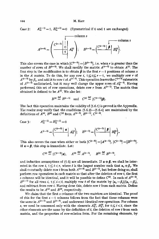
A ( S - Z ) ~ 4 R{s-1) Case 2: --,s . . . . ,~ = 0 (Symmetr ica l if 0 and I are exchanged)
A (s-l) ~__
column s column s
This also covers the case in which [C(*-xl[ = IB('-I)I, i.e. when r is grea ter t han the number of rows of B (s-l). We shall modi fy the ma t r i x A I*-~) to obta in A (~1. The first s tep in the modif icat ion is to obta in p in the first r - - t posi t ions of column s in the A mat r ix . To do this, for any row i, t < i < r - - t , we mul t ip ly row r of A (,-11 b y flo and add it to row i of A('-*I. This opera t ion leaves the C (~-~) submat r ix of A (*-1) undis turbed, bu t it m a y well change the uppe r rows of A~ '-xl. Hav ing per fo rmed this set of row operat ions, delete row r f rom A ('-x). The ma t r i x thus ob ta ined is defined to be A I*l. We also let:
B(,) d,f ]~) = B (~-1) and C(,) d,f (C(,_1) .
The fact this opera t ion main ta ins the va l id i ty of (5.6.t) is p roved in the Appendix. The reader m a y ver i fy t ha t the condit ions (5.6.2)--(5.5.4) are ma in ta ined b y the definitions of A (*), B (*) and C l0 f rom A (~-1), B (~-1), C (*-x).
A (s-Z) _ _ R(s-1) _ _ n Case 3 : --,s -- ~rs - - ~
1,__(C" 1',' I This also covers the case when ei ther or bo th [C(S-1) I "= [A(S-1)l, [C(S-1) I = [B(*-*']. I f = = / L this s tep is immedia te . Let :
C(,) def___ (C(,_X)la), A( 0 aa= A(,_z) ' B(~) da= B(,_I) '
and induct ion assumpt ions of (5.6) are all immedia te . I f = :#~, we shall be inter- ested in the row t, t =< t < r, where t is the largest n u m b e r such t ha t ott :#fit. We shall eventua l ly delete row t f rom both A (s-l} and B (s-x), bu t before doing so, shall per form row operat ions in each ma t r i x so t ha t a f ter the deletion of row t, the first s columns will be identical, and it will be possible to define C (s). In each of A (s-l), B (s-l) for all rows i, t ~ i < t, mul t ip ly row t of the ma t r i x b y (oq--fl~)[(ot t --fit), and sub t rac t f rom row i. Hav ing done this, delete row t f rom 6ach mat r ix . Define the results to be A C*) and B (s), respectively.
We claim tha t the first s columns of the two matr ices are identical. The proof of this for the first s - t columns follows f rom the fact t ha t those columns were the same in A (s-ll and B (s-ll, and underwent ident ical row operations. For column s, we need be concerned only wi th the elements A~ I, B~ I, for t ~ i < t, since the o ther elements are the same b y the definit ion of t, the deletion of row t f rom each mat r ix , and the proper t ies of row-echelon form. For the remaining elements, b y
Affine Relationships Among Variables of a Program 145
virtue of the row operations we performed, we have:
A~ ) = o q - - \ c r -- cot--fit = f l i \ cr ] ~ ' t=
Thus, we can define C (') to be the submatr ix of either A (s) or B (s) consisting of the first s columns of the first r - 2 rows.
(It is in this case tha t we m a y arrive at a mat r ix C I') with no rows, but s columns. See (5.6.4).)
Given the above definitions of A (*), B ('), and C I'), the "continued correctness of (5.5.t) will be shown in the Appendix, and (5.6.2)--(5.6.4) are left to the reader.
6. Some Examples
6.1 Pathological Flow Properties
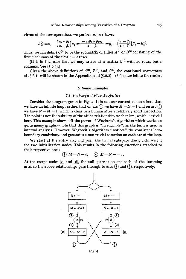
Consider the program graph in Fig. 4. I t is not our current concern here that we have an infinite loop; rather, tha t on arc (~) we have M -- N = t and on arc (~) we have N -- M = t, which is clear to a human after a relatively short inspection. The point is not the subtlety of the affine relationship mechanism, which is trivial here. This example shows off the power of Wegbreit 's Algorithm which works on quite messy graphs- -note tha t this graph is " irreducible", as the te rm is used in interval analysis. However, Wegbreit 's Algorithm "no t ices" the consistent loop- boundary conditions, and generates a non-trivial assertion on each arc of the loop.
We s tar t at the entry arc, and push the trivial subspace down until we hit the two initialization nodes. This results in the following assertions at tached to their respective arcs:
(~ M - - N = 1 , (~) M - - N : - - t .
At the merge nodes [ ] and I-d], the null space is on one each of the incoming ares, so the above relationships pass through to arcs C) and ~), respectively.
[]
I .... I I .... I
[M~-N+I ] [ N,-M+I I
/ \ j|
Fig. 4
[]
t46 M. Karr
| Fig. 5
Using the formula (4.7), we get:
from node I-a-I: c| = t + t �9 (--2) = --1,
from node I-b]: c~ = - - t + ( - - t ) (--2) = t .
Thus we get assertions
(~ M--N----I, @ M - - N = t .
Now, we are at the point where we must perform affine unions at [ ] and [~].
D : <(t, - t ) , 1> ~ <(1, - t ) , t> [ ] :<0, - t ) , - t > ~ <(t, - t ) , -1>.
I t is obvious what we get as unions here, so we postpone an example of the com- putation for a more enlightening case. Note that the unions specify the affine assertions which are already on arcs (~) and (~) respectively, so that the algorithm terminates.
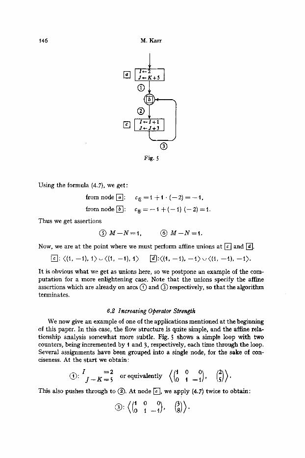
6.2 Increasing Operator Strenglh We now give an example of one of the applications mentioned at the beginning
of this paper. In this case, the flow structure is quite simple, and the aifine rela- tionship analysis somewhat more subtle. Fig. 5 shows a simple loop with two counters, being incremented by I and 3, respectively, each time through the loop. Several assignments have been grouped into a single node, for the sake of con- ciseness. At the start we obtain:
J--K-----5 or equivalently t -- ' "
This also pushes through to (2"). At node [~], we apply (4.7) twice to obtain:
o _~
Affine Relationships Among Variables of a Program t47
Then, we are back at node [~], where we must perform the disjunction of the predicates on arcs ~ ) and ~), i.e.
(loO o t - - 1 v t - - t "
We now run through the algorithm of Section 5.4. Two quick applications of case t, followed by the trivial application of case 3 leave A 181 and B c8) equal to the original A and B, respectively. We have
At column four, we have a non-trivial case 3. In the notation of that section,
e = ( 2 , 5 ) and ~ ---- (3, 8).
The last row on which ~ and p differ is given by t ---- 2. Observe :
(~, - , r - , 8 , ) = (2 - 3)/(5 - 8 ) = t /3.
In each of the matrices, we multiply the second row by t/3, and subtract it from the first row. We then delete the second row:
(I -113 tl3 2-513) v(1 - t / 3 t/3 3 - 8 / 3 ) = ( t - t / 3 t/3 t/3).
Thus the assertion on ~ ) is:
Q : ((t - t / 3 t/3), t /3 ) or equivalently 3 I - J + K - - t .
Now we consider the effect of the assignment node at [7]. For clarity, we now consider the assignments one at a time. After I<--I + t, we have:
c = 1/3 + t �9 t = 4/3, A is unchanged.
However, after J , , - J + 3, we have:
c = 4/3 + ( - - t/3) �9 3 = t13, A is unchanged.
In other words, the two assignments have a combined effect of nil on the assertion, and we also obtain:
O : ((t - t / 3 t/3), 1/3).
We are at node [ ] a third time, and must calculate the linear disjunction:
o (t - t / 3 t/3 t /3)v I - t "
For s ---- t , we apply case 1, but with s ---= 2, we must use case 2. This requires tha t in the second argument, we subtract one third times the second row from the first, and delete the second. This yields:
(t -113 tl3 2 -5 /3 )=0 - t / 3 t/3 t/3).
148 M: Karr
For s ----3 and 4 we have trivial applications of case 3, so that we again wind up with the same result for (.2~, and may terminate the algorithm.
Hence, except for the undrawn arc internal to node e~), inside the loop have the relationship:
3 I - - J + K = t , i.e., J = K + 3 I - - I ,
This has been done without having to intelligently hypothesize an invariant relationship; affine disjunction takes care of this.
6.3 Constant Detection
Given the relationships (A, e ) on a given arc, in order to determine whether a linear form B - V is a constant, merely a t tempt to express B as a linear combina- tion of the rows of A. If this is not possible, then we cannot conclude, at least on the basis of VEker (A, e ) , tha t B �9 V is a constant. This is a direct consequence of the theory of the general solution of simulataneous equations, which says that under this linear independence, the system
(6,/
has fewer solutions than ( A , e ) , i.e. there are two solutions V x, V~ for ( A , e ) which differ: B V 1 =VBV,, so that at most one is a solution to (6.1). On the other hand, if
B - ~ ~, ~iAi (m = n u m b e r of rows of A), i = 1
then
B . V = 2 i A i �9 V = ).i(Ai �9 V) = ;tic i, i i=1 i=1
so tha t B �9 V is an obvious constant.
Since A is in row-echelon form, trying to find the desired linear combination is trivial: merely append (B, 0) to (A, e ) and do row reductions. If the last row goes to zero in the first n entries, the negative of the desired constant,
- - ~, )tic~, i = 1
appears in the n + t st column; otherwise, a new dependent column emerges, and B is linearly independent of the rows of A. In particular, a variable, ~, is a con- s tant r j is a dependent variable of A, and the (unique) row i in which column/" is non-zero (i =0-1(i)) is 0 everywhere except the ~.th position. The constant is given in the special case by:
cdA ~ j.
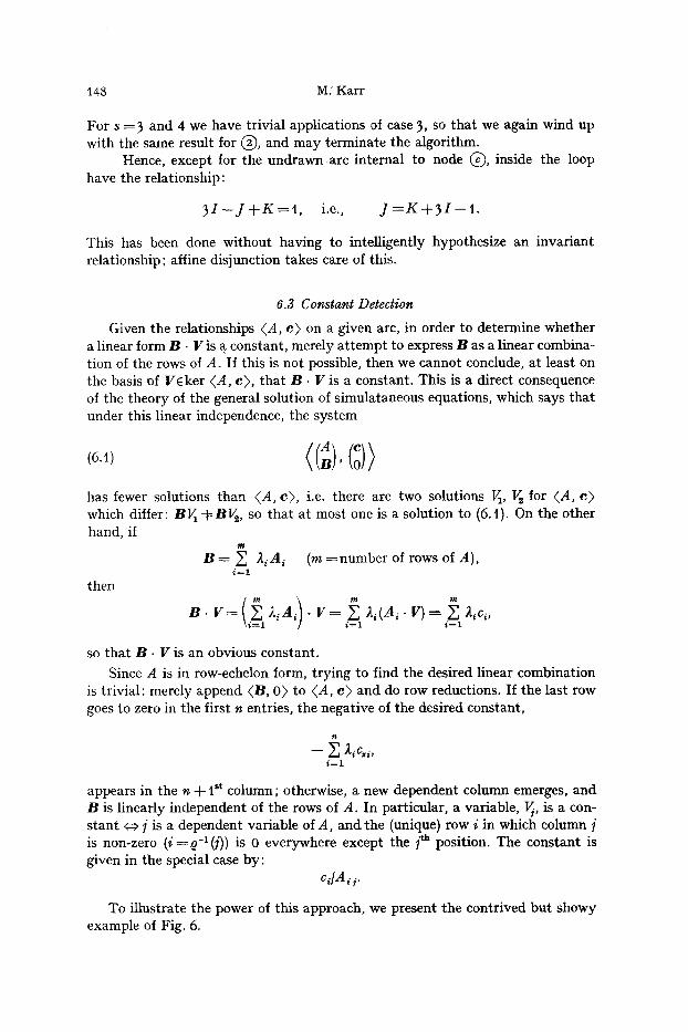
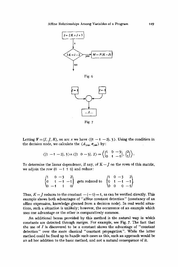
To illustrate the power of this approach, we present the contrived but showy example of Fig. 6.
Affine Relationships Among Variables of a Program
[I~2K+J+3 l X
n o
149
Fig. 6
Fig. 7
Letting V=(I, J, K), on arc x we have ((t - - t --2) , 3). Using the condition in the decision node, we calculate the (Ayes, eyes) by:
( ( t - - t - - 2 ) , 3 ) ^ ( ( t 0 - - 3 ) , 2 ) = ( ( t 0 0 ,
To determine the linear dependence, if any, of K - J on the rows of this matrix, we adjoin the row (0 --1 I 0) and reduce:
(i !) (io i) t - - t - - gets reduced to t - - t . - - t 1 0 0
Thus, K - J reduces to the constant - - ( - - t) = t , as can be verified directly. This example shows both advantages of "affine constant detect ion" (constancy of an affine expression, knowledge gleaned from a decision node). In real world situa- tions, such a situation is unlikely; however, the occurrence of an example which uses one advantage or the other is comparat ively common.
An additional bonus provided by this method is the natural way in which constants are detected through merges. For example, see Fig. 7. The fact tha t the use of I is discovered to be a constant shows the advantage of "cons tan t detect ion" over the more classical "cons tan t propagat ion" . While the lat ter method could be fixed up to handle such cases as this, such an approach would be an ad hoc addition to the basic method, and not a natural consequence of it.
t50 M. Karr
A p p e n d i x
Proo/ o/ (6.4) Let (A o, Co) de~ (A1, oi)i V (A2, c~). To show that (Ao, Co) = (A, e), we merely show that the kernels are equal. For any B, d, and VEker (B, d):
(t) ker (B, d) ={~<V, - - t> + WIWEker B, 2EF}.
To prove this, note that ker (B, d) is at least this big, and that the set is closed under addition and under multiplication from F.
Pick any V~Eker <Ai, ci>, i =1 , 2. Then ohVa+co~V~Eker <A, c>, because affine spaces (in particular, the union) are closed under weighted average ([t], p. 422). Generalizing the above formula slightly, we observe that:
(2) ker (A, c ) - -{2(o~1~ +co~ V ~, - - t ) + l ~ t +H721W~Eker A ~, ~tEF}.
Again, the kernel may be seen to be at least this big; and the above set is a linear subspace. But since --1 = --oJ x --o J2, we have:
ker (A, e) = [;tcoi (~ , -- t ) + l~d I $t~Eker Ai, 2 ~F
-----{X1 + X , IXiEker (Ai, e~)}
--ker (Ao, co).
The first equality is mere rearrangement of (2), the second uses (t), and the third is a property of the sum of linear subspaces ([t], p. t98). The identity of the kernels completes the proof.
Validity o/ (5.6.1) /or Cases 2 and 3 We first observe that removing rows from the matrices enlarges the spaces,
so that we immediately see that
ker A (s-i) + ker B (*-1} (ke r A (s) + ker B (sl
If we can prove equality here, induction will immediately give us (5.6A). Equality may be proved by showing that the dimensions are equal, which in turn may be shown by proving that the ranks of the matrices are equal. Using (5.6.3), we must show:
IA I*-xl v B(s-x) I = IA('I v BI')[
In case 2, view the deleted row as a one row matrix D, and observe that:
A Is-x) =AI')^ D,
(*) IAI') ̂ D[ ----IaC')l + t .
Notice that column s will be an independent column of AI')A B('); since D has a t in this column and 0 in previous columns,
(?) IAISl ̂ Bt') ̂ DI =IAr ^ BC') I + t .
Affine Relationships Among Variables of a Program 15t
Hence
[A(,-1) v B(,-1)I _ ]A(,-1) v B(,) I ----- [A('-x)[ + [ B (s)] --]At~)A n A B ts)]
=IA~')I +a + I B ( ' ) I - (IA(S)A B (*)] +4)
= [A (') v B(') I
(because B (') = B Is-t))
(dimension formula, (,))
(by (,), (t))
(cancellation of ones, dimension formula).
(The required dimension formula may be found in [t ], p. 235, Corollary 2.) This proves equality ior case 2.
For case 3, the reasoning is quite similar. Let D be the row removed from A Cs-ll and E be the row removed from B Is-x). In addition to (.), we have:
B ('-1) = B (s) A E,
(**) I BC') ̂ E I --[B(')[ +4. Observe that both column s and column q-1 (t) (the position of the first dement of this row in C (s-l~) are independent columns of A (~) and B(S); also, that tile two columns will be dependent columns of D A E (think about doing the row reductions necessary to put this in canonical form). We conclude that:
(r [A(~)^B(~)ADAEI=[A(S)^B(S)[+[D^EI=IA(OAB(~[+2. Thus,
IAI,-~) v Bt'-*~I --I(A, ~'~ ̂ D) v (B ~'} A E)l
=IAr + t + IB(')I + a - ( I a ( ' l ^ B(') I + 2 ) = [AO~v B(O I
(by (,), (**))
(dim. formula, (,), (**), (tt))
(cancellation, dimension formula).
This completes the proof that the algorithm for linear disjunction is correct.
R e f e r e n c e s
1. MacLane, S., Birkhoff, G. : Algebra. New York: MacMillan 1967 2. Munkres, J. R. : Elementary linear algebra. Reading (Mass.): Addison-Wesley
t964 3. Floyd, R. : Assigning meanings to programs. In: Schwartz, J. (ed.): Mathematical
aspects of computer science 19. Providence (R.I.): American Mathematical Society t967, p. t9--32
4. Wegbreit, Ben: Property extraction in well-Founded property sets. Center for Research in Computing Technology, Harvard University, Cambridge (Mass.) and Computer Science Division, Bolt, Beranek, and Newman, Inc., Cambridge (Mass.), February a973
5. Karr, M.: Gathering information about Programs. Massachusetts Computer Associates, Inc., (In preparation)
6. Birkhoff, G. : Lattice theory. Colloquium Publication XXV, 3. Ed., Providence (R.I.): American Mathematical Society t973
Michael Karr Massachusetts Computer Associates Inc. Lakeside Office Park Wakefield, Mass. 0t 880 U.S.A.