lecture 3-2 summarizing relationships among variables ©
TRANSCRIPT

Lecture 3-2Lecture 3-2
Summarizing Summarizing Relationships Relationships
among variablesamong variables
©
Numerical measures of Numerical measures of summarizing the summarizing the
relationship between two relationship between two variablesvariables
To think of what numerical measures we need to represent relationships between variables, see the following three pairs of scatter plots.
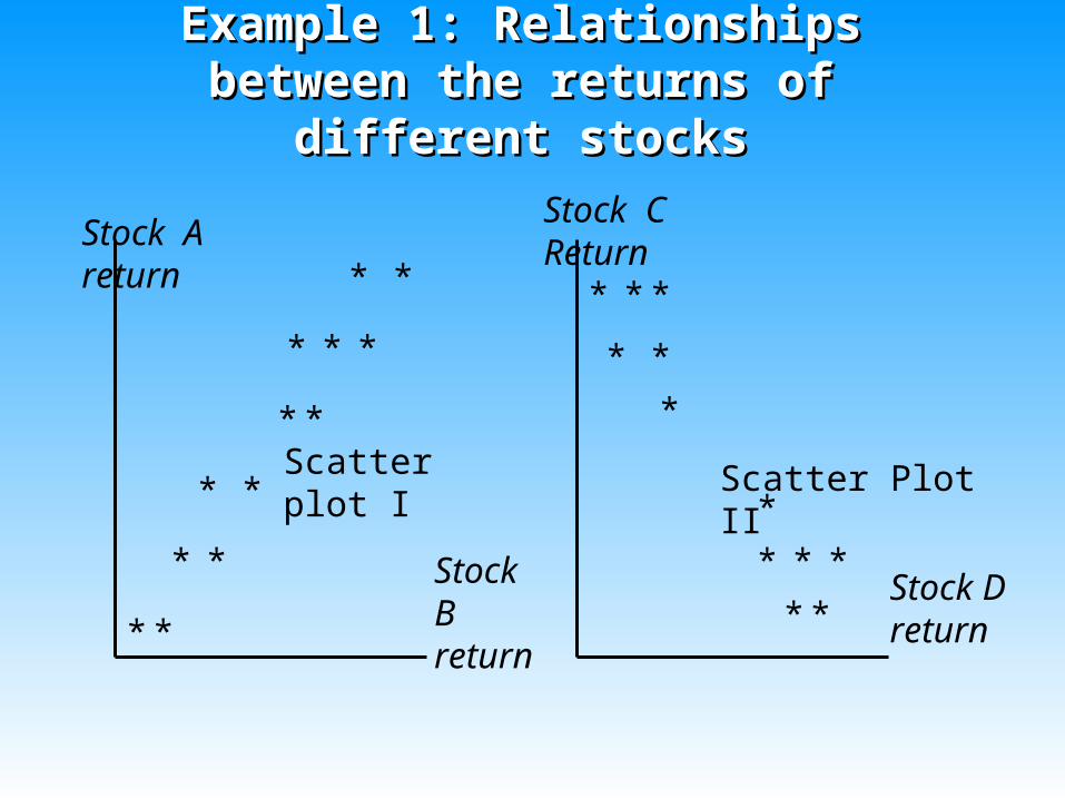
Example 1: Relationships Example 1: Relationships between the returns of different between the returns of different
stocksstocks
Stock B return
Stock A return *
* *
*
*
*
*
*
*
*
*
*
*
Stock D return
Stock C Return
*
* *
*
*
*
*
*
*
*
*
*Scatter plot I Scatter Plot II

Example 1 (Continued)Example 1 (Continued) Scatter Plot I shows a positive
relationship while scatter plot II shows a negative relationship.
We need a numerical measure that shows the direction of the relationship.
For this purpose, we use “Covariance”

Example 2: Relationships Example 2: Relationships between advertisement between advertisement spending and revenuespending and revenue
Advertisement and revenue product I
0
10000
20000
30000
40000
50000
60000
70000
80000
0 50 100 150 200
Advertisement spending
Rev
enue
Advertisement and revenue Product II
0
5000
10000
15000
20000
25000
30000
35000
0 20 40 60 80 100 120
Advertisement spending
Rev
enue
Product I shows a clear linear relationship between the advertisement spending and revenue, while product II does not show much of a relationship. We need to have a numerical measure that shows the strength of linear relationship between two variables. We use “Correlation Coefficient”

Example 3: Number of Example 3: Number of promotion and salespromotion and salesProduct A: Promotion and sales
0
500,000
1,000,000
1,500,000
2,000,000
2,500,000
0 5 10 15 20 25
Number of promotions
Sal
es
Product B: Promotion and Sales
0
500,000
1,000,000
1,500,000
2,000,000
2,500,000
0 5 10 15 20 25
Number of promotions
Sal
es
Promotion seems to be more effective for Product A than product B in the sense that additional promotion brings greater increase in revenue (i.e., the “slope” is steeper). To measure the effectiveness of the promotion, we use “Regression Analysis”
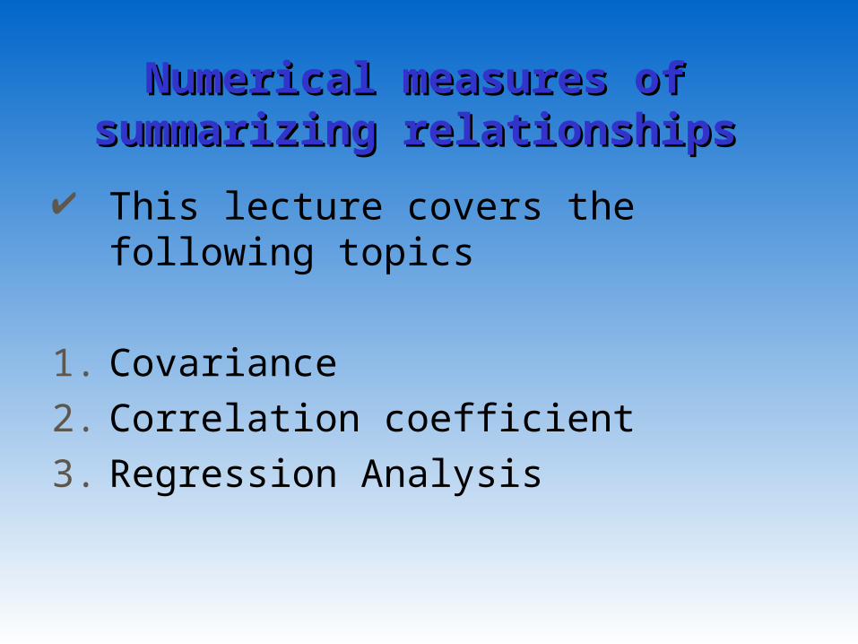
Numerical measures of Numerical measures of summarizing relationshipssummarizing relationships
This lecture covers the following topics
1. Covariance2. Correlation coefficient3. Regression Analysis

CovarianceCovariance Covariance is a numerical measure that
shows the direction of the relationship between two variables.
Covariance is one of the most fundamental numerical measures of the relationship between two variables. It will appear in many areas (i.e., computation of returns of a portfolio of stocks)
In the following slides, we will learn the logic behind the derivation of covariance.
How to measure the How to measure the direction of the relationshipdirection of the relationship
X
Y
x
y*
* *
*
*
*
*
*
*
*
*
*
*
Positive Relationship
W
Z
w
z
*
* *
*
*
*
*
*
*
*
*
*
Negative relationship
*
**
*
**
Box I
Box IIBox III
Box IVBox I
Box IIBox III
Box IV

How to measure the How to measure the direction of the relationshipdirection of the relationship
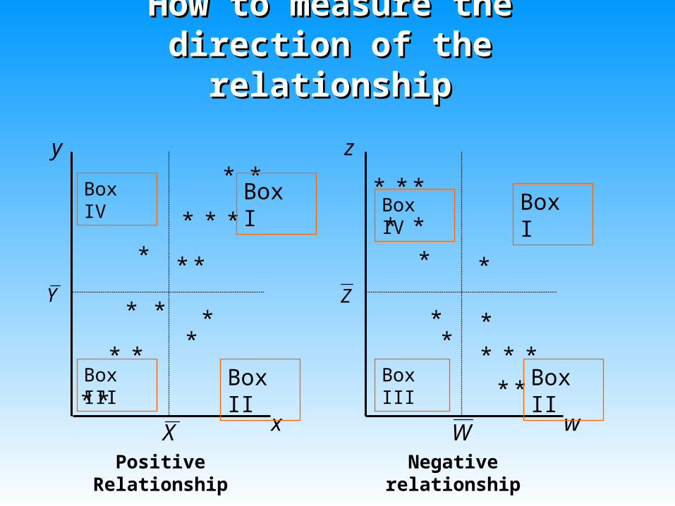
From the previous two scatter plots, notice that:
1. When two variables show a positive relationship, there are more data points in Box I and Box III, than in Box II and Box IV
2. When two variables show a negative relationship, there are more data points in Box II and Box IV, than Box I and Box III.
We use these facts to measure the direction of the relationship.
How to measure the How to measure the direction of the relationship: direction of the relationship:
ExampleExample
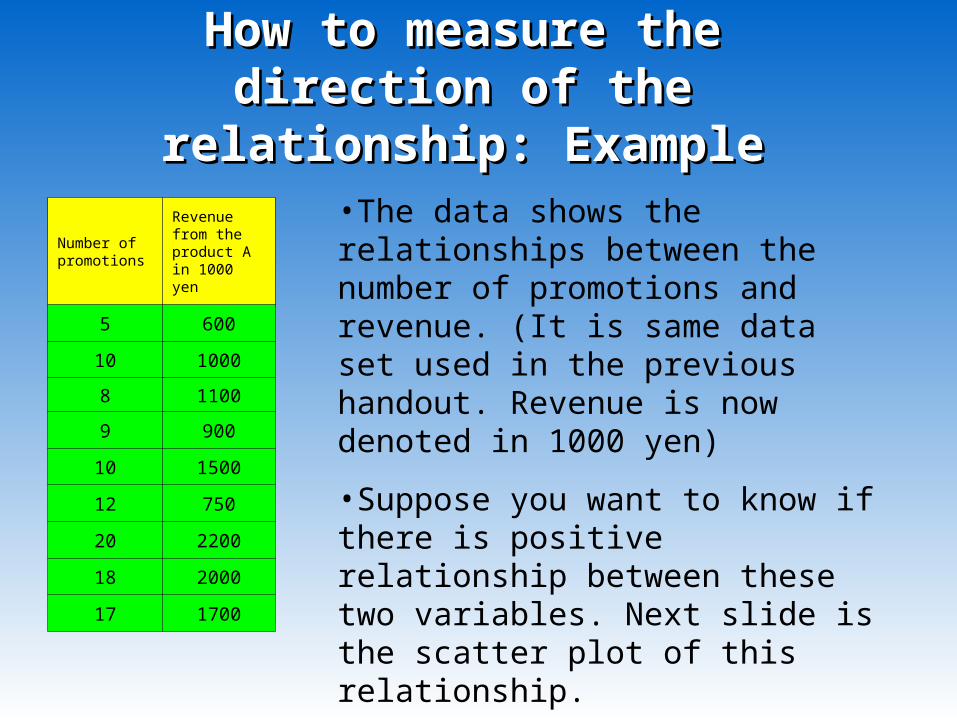
Number of promotions
Revenue from the product A in 1000 yen
5 600
10 1000
8 1100
9 900
10 1500
12 750
20 2200
18 2000
17 1700
•The data shows the relationships between the number of promotions and revenue. (It is same data set used in the previous handout. Revenue is now denoted in 1000 yen)
•Suppose you want to know if there is positive relationship between these two variables. Next slide is the scatter plot of this relationship.

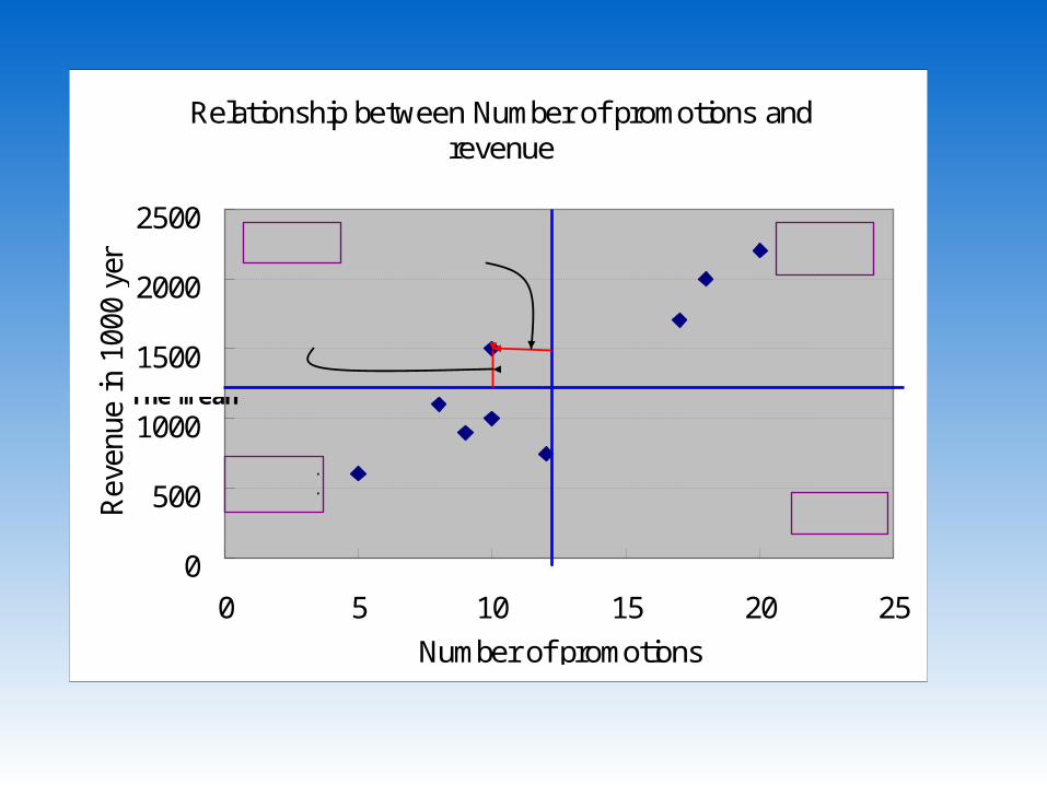
How to measure the How to measure the direction of the relationship: direction of the relationship:
Example, contdExample, contd
Relationship between Number of promotions andrevenue from product A
0
500
1000
1500
2000
2500
0 5 10 15 20 25
Number of promotions
Reve
nue
in 1
000
yen
Box I
Box II
Box IV
Box III
The mean=12.11
The mean = 1305.6
• Number of promotions and revenue appears to have a positive relationship.
• Notice that most of the data points are either in Box I or Box III
• What can we say about Box I and Box III? See the next slide

How to measure the How to measure the direction of the relationship: direction of the relationship:
Example, contdExample, contdRelationship between Number of promotions and
revenue
0
500
1000
1500
2000
2500
0 5 10 15 20 25
X: Number of promotions
Y: R
even
ue in
100
0 ye
n
Box I
Box II
Box IV
Box III
The mean of X=12.11
The mean of Y =1305.6
• For each data point, you can compute the distances from the means.
• Then we can notice that, for any data points in Box I, both of the distances are positive.
• For any data points in Box III, both of the distances are negative.
See the next slide
Distance from the mean of X = (X- the mean of X)
Distance from the mean of Y = (Y- the mean of Y)

Relationship between Number of promotions andrevenue
0
500
1000
1500
2000
2500
0 5 10 15 20 25
Number of promotions
Rev
enue
in 1
000
yen
Box I
Box II
Box IV
Box III
The mean of X
The mean of Y
Box I Distances from themeans are both positive
Box III: Distances fromthe means are bothnegative

How to measure the How to measure the direction of the relationship: direction of the relationship:
Example, contdExample, contd For a data point in Box I, distances from the
means are both positive. That is, both (X- ) and (Y- ) are positive.
Therefore, if we multiply the two distances together, we will have a positive number
For a data point in Box III, distance from the means are both negative. That is (X- ) and (Y- ) are both negative.
Therefore, if we multiply the two distances together, we will again have a positive number.
Now, what we can say about Box II and Box IV? See next slide.
YX
XY
Relationship between Number of promotions andrevenue
0
500
1000
1500
2000
2500
0 5 10 15 20 25
Number of promotions
Rev
enue
in 1
000
yen
Box I
Box II
Box IV
Box III
The mean
The mean
Positive distance
Negativedistance

How to measure the How to measure the direction of the relationship: direction of the relationship:
Example, contdExample, contd
For any points in box II and box IV, one distance will be positive and the other distance will be negative. So if we multiply them together, we will have a negative number.

How to measure the How to measure the direction of the relationship: direction of the relationship:
Example, contdExample, contd Consider, for each data point, you compute the
distances from the means, then multiply them together. Further, consider you sum all the multiplied distances together. If the resulting number is positive, this roughly indicates that there are more data points in Box I and Box III than Box II and Box IV. This in turn indicates that the data shows positive relationship. If the resulting number is negative, this indicates a negative relationship.
This is the basic idea of measuring the direction of the relationship between two variables, and this is the first step to compute “Covariance”.

Computation of the Sample Computation of the Sample CovarianceCovariance
The sample covariance is computed in the following way.
1. Compute the mean for each variable.2. For each observation, and for each variable,
compute the distances from the means, i.e. compute (X- ) and (Y- ). Then multiply them together.
3. Sum all the multiplied differences.4. Divide the sum of the multiplied differences by
n-1, (that is the number of observations minus 1).
XY
Computation of Sample Computation of Sample covariancecovarianceExerciseExercise
Open “Computation of Covariance” data set.
Using data on the sheet “data 1”, compute the covariance between the number of promotions and the revenue.

Exercise, contdExercise, contd
The covariance between the number of promotions and revenue is 2561.8
Positive covariance indicates that the number of promotions and revenue have a positive relationship.
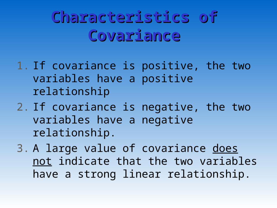
Characteristics of Characteristics of CovarianceCovariance
1. If covariance is positive, the two variables have a positive relationship
2. If covariance is negative, the two variables have a negative relationship.
3. A large value of covariance does not indicate that the two variables have a strong linear relationship.

A note on CovarianceA note on Covariance
One may be tempted to conclude that if the covariance is larger, the relationship between two variables is stronger (in the sense that they have stronger linear relationship)
However, this is not true. To see this, go over the next example.

A note on Covariance, A note on Covariance, example example
Open the data “Computation of Covariance”, work sheet “data 2”. Compute the covariance between variable X and Y.
(The data 2 is in fact the same as data 1. Only the difference is, the revenue is measure in 1000 yen for data 1, while it is measure in 1 yen for data 2.)

Example, contdExample, contd
The covariance for data 2 is 2561805. This compares the covariance for data 1 which was 2561.8.
Even if data 1 and data 2 show exactly the same relationship, covariance for data 2 is much larger. This is simply because the unit of measurement for revenue is different between data 1 and data2.
This shows that a larger covariance does not mean a stronger relationship. (In this particular example, relationship is exactly the same.)
To show the strength of the relationship, we use “Correlation coefficient”.

Sample Correlation Sample Correlation CoefficientCoefficient
The measure of the strength The measure of the strength of linear relationshipof linear relationship
Correlation coefficient between X and Y, denoted as rxy, is computed as
Y) ofdeviation (Standard*X) ofdeviation (Standard
Y) and Xbetween e(Covariancxyr

Characteristics of Characteristics of Correlation CoefficientCorrelation Coefficient
1. The correlation coefficient ranges from –1 to +1 with,• rxy = +1 indicates a perfect positive linear relationship:
the X and Y points would plot an increasing straight line.• rxy = 0 indicates no linear relationship between X and Y.• rxy = -1 indicates a perfect negative linear relationship:
the X and Y points would plot a decreasing straight line.2.2. Positive correlationsPositive correlations indicate positive or increasing
linear relationships with values closer to +1 indicating data points closer to a straight line and closer to 0 indicating greater deviations from a straight line.
3.3. Negative correlationsNegative correlations indicate decreasing linear relationships with values closer to –1 indicating points closer to a straight line and closer to 0 indicating greater deviations from a straight line.
4. Correlation coefficient is not the slope of the relationship.

Correlation CoefficientCorrelation CoefficientExerciseExercise
Open “Computation of Covariance”. Compute correlation coefficient between the number of promotion and revenue for both data 1 and data 2.
Correlation Coefficient Correlation Coefficient exercise exercise
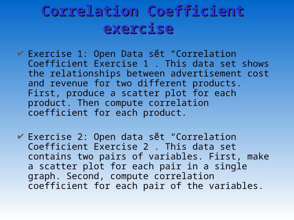
Exercise 1: Open Data set “Correlation Coefficient Exercise 1”. This data set shows the relationships between advertisement cost and revenue for two different products. First, produce a scatter plot for each product. Then compute correlation coefficient for each product.
Exercise 2: Open data set “Correlation Coefficient Exercise 2”. This data set contains two pairs of variables. First, make a scatter plot for each pair in a single graph. Second, compute correlation coefficient for each pair of the variables.

Exercise 1, AnswerExercise 1, AnswerProduct I; Advertisement cost and Revenue
0
10000
20000
30000
40000
50000
60000
70000
80000
0 50 100 150 200
Ad cost
Rev
enue
CorrelationCoefficient=0.95
Product II: Advertisement Cost and revneue
0
5000
10000
15000
20000
25000
30000
35000
0 20 40 60 80 100 120
Ad cost
Rev
enue
CorrelationCoefficient = 0.05
Product I shows strong positive linear relationship between advertisement cost and revenue. Correlation coefficient is 0.95, which is close to 1. Product II does not show much linear relationship. The correlation coefficient is close to 0.05, which is close to 0.

Exercise 2 (Answer)Exercise 2 (Answer)Correlation Coefficient Exercise 2
-30
-20
-10
0
10
20
30
0 2 4 6 8 10 12 14 16 18
Pair IPair II
Correlation Coefficient=-1
Correlation Coefficient =- 1

Correlation Coefficient Correlation Coefficient Exercise 2 (Answer)Exercise 2 (Answer)
First, for both pairs, the correlation coefficients are -1. This means that the relationships are perfectly (negatively) linear for both pairs of variables.
Also note that, even though the slope for the pair I is much steeper, the correlation coefficients are the same for both pairs. This shows that correlation coefficient is not the slope of the relationship.

Correlation CoefficientCorrelation Coefficient
To have more idea about the coefficient correlation, see the following slides

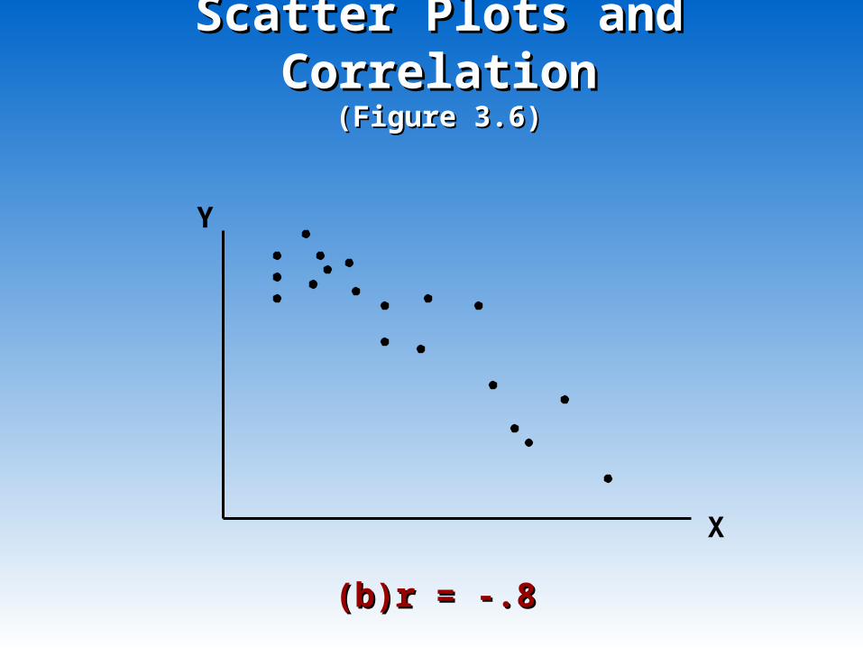
Scatter Plots and Scatter Plots and CorrelationCorrelation
(Figure 3.6)(Figure 3.6)
X
Y
(a) r = .8(a) r = .8
X
Y
(b)r = -.8(b)r = -.8
Scatter Plots and Scatter Plots and CorrelationCorrelation
(Figure 3.6)(Figure 3.6)

Scatter Plots and Scatter Plots and CorrelationCorrelation
(Figure 3.6)(Figure 3.6)
X
Y
(c) r = 0(c) r = 0
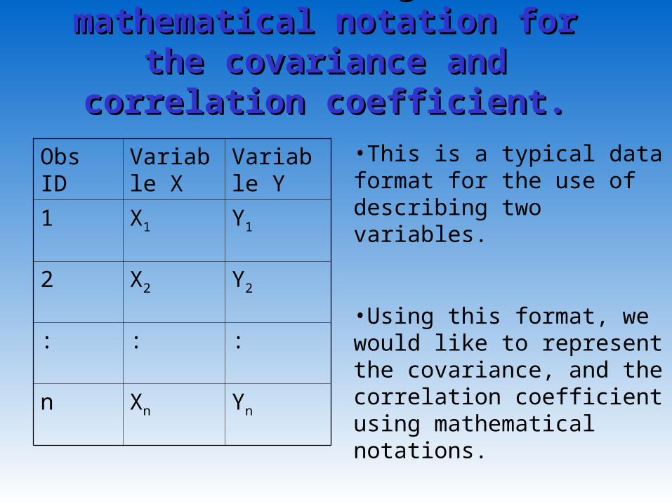
Understanding the Understanding the mathematical notation for mathematical notation for
the covariance and the covariance and correlation coefficient.correlation coefficient.
Obs ID Variable X
Variable Y
1 X1 Y1
2 X2 Y2
: : :
n Xn Yn
•This is a typical data format for the use of describing two variables.
•Using this format, we would like to represent the covariance, and the correlation coefficient using mathematical notations.
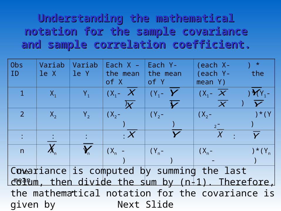
Understanding the mathematical Understanding the mathematical notation for the sample covariance notation for the sample covariance and sample correlation coefficient.and sample correlation coefficient.
Obs ID
Variable X
Variable Y
Each X –the mean of X
Each Y- the mean of Y
(each X- ) * (each Y- the mean Y)
1 X1 Y1 (X1- ) (Y1- ) (X1- )*(Y1- )
2 X2 Y2 (X2- ) (Y2- ) (X2- )*(Y2- )
: : : : :
n Xn Yn (Xn - ) (Yn- ) (Xn- )*(Yn- )
The mean
XXX
X
XXX
Y
Y
Y
Y
Y
Y
Y
Covariance is computed by summing the last colum, then divide the sum by (n-1). Therefore, the mathematical notation for the covariance is given by Next Slide

Mathematical Notation for Mathematical Notation for the sample covariancethe sample covariance
1
))((
1
))(())(())((),(
1
2211
n
YyXx
n
YyXxYyXxYyXxsyxCov
n
iii
nnxy
X
The mathematical notation for covariance between variable X and variable Y, denoted by either Cov(X,Y) or sxy, is given as
where xi and yi are the observed values, and are the sample means, and n is the sample size.
Y

Mathematical Notation for Mathematical Notation for the sample correlation the sample correlation
coefficientcoefficient
yxxy ss
yxCovr
),,(
The sample correlation coefficient, rsample correlation coefficient, rxyxy, , is computed by the equation
Sx is the standard deviation of variable X. Sy is the standard deviation for variable Y.

3. Ordinary Least Square 3. Ordinary Least Square estimationestimation
-A Regression Analysis--A Regression Analysis-
0
500,000
1,000,000
1,500,000
2,000,000
2,500,000
0 5 10 15 20 25Number of promotions
Rev
enue
Product AProduct BProduct CProduct A trendProduct B TrendProduct C Trend
•This is the scatter plot we saw in Lecture 3-1. From the graph, we can see that promotion is more effective for product A than product B.
•Then, how do we measure the effectiveness of promotions?
•Correlation coefficient cannot be used for this purpose since it is not the measure of the slope

Ordinary Least Square Ordinary Least Square estimationestimation
A Regression AnalysisA Regression Analysis
0
500,000
1,000,000
1,500,000
2,000,000
2,500,000
0 5 10 15 20 25Number of promotions
Reve
nue
Product AProduct BProduct CProduct A trendProduct B TrendProduct C Trend
To measure the effectiveness of promotion for each product, we use regression analysis.
In this handout, we will talk about a type of regression analysis called “Ordinary Least Square Estimation”

Ordinary Least Square Ordinary Least Square EstimationEstimation
Product A: Promotion and sales
0
500,000
1,000,000
1,500,000
2,000,000
2,500,000
0 5 10 15 20 25
Number of promotions
Reve
nue
Product A: Promotion and sales
y = 99060x + 105827
0
500,000
1,000,000
1,500,000
2,000,000
2,500,000
0 5 10 15 20 25
Number of promotions
Reve
nue
•Ordinary Least Square (OLS) estimation is a method to find a linear equation that best fits the data. Left hand graph is a simple scatter plot of the relationship between the number of promotions and the revenue from product A. The right hand side graph shows the OLS estimation of the linear relationship between the number of promotion and revenue for the product A.
•Next several slides show the logic behind the OLS estimation.

Ordinary Least Square Ordinary Least Square EstimationEstimation
(Two variable case)(Two variable case)Ordinary Least Square EstimationOrdinary Least Square Estimation assume that the number of promotions and the revenue from the product has the following relationship.
More generally, ordinary least square estimation assume that, between variable Y and variable X, there is a following linear relationship.
An equation, like this, that describes a relationship among variables is called a “model”, or “regression equation”. The model above contains two parameters, 0 and 1. They are called the model coefficients. The coefficient 0, is the intercept on the Y-axis and the coefficient 1 is the slope. (The slope is the change in Y for every unit change in X.)
XY 10
)promotions ofNumber ((Revenue) 10
Ordinary Least Square Ordinary Least Square EstimationEstimation
(Two variable case)(Two variable case)
Ordinary Least Square Estimation is a method to find (estimate) the values for β0 and β1 that fit the equation to the data “best”.
The criteria to choose (estimate) the values for β0 and β1 is described in the following slides.

Ordinary Least Square EstimationOrdinary Least Square EstimationCriteria to estimate the parameter valuesCriteria to estimate the parameter values
X (number of promotion)
Y (Sales from Product A)
ei
XY 10
(xi, yi)
Vertical distance from the equation to ith data point
We choose (estimate) the values for β0 and β1 so that the sum of the squared (vertical) distances from the equation to each data point is minimized. (Therefore, this estimation is called ordinary least square estimation.) Excel automatically estimates these values.

Ordinary Least Square Ordinary Least Square Estimation Using Excel, Estimation Using Excel,
ExampleExampleProduct A: Promotion and sales
y = 99060x + 105827
0
500,000
1,000,000
1,500,000
2,000,000
2,500,000
0 5 10 15 20 25
Number of promotions
Rev
enue
Excel can estimate the linear equation model, and draw the line at the same time. The estimated β0 =105827, and β1=99060.
Exercise: Open Data “OLS Exercise 1-Promotion and Sales” and reproduce this figure.

Things we can do with Things we can do with OLSOLS
Using the estimated equation, we can
1. Find the effect of promotion on the revenue for product A.
2. Forecast revenue for different number of promotions.
3. Find the number of promotions necessary to achieve your sales goal.

Effect of promotion on the Effect of promotion on the sales of product Asales of product A
Product A: Promotion and sales
y = 99060x + 105827
0
500,000
1,000,000
1,500,000
2,000,000
2,500,000
0 5 10 15 20 25
Number of promotions
Rev
enue
The estimated slope parameter β1 is the estimated effect of promotion on the revenue from product A. β1=99,060 means that if you increase the number of promotion by one, the revenue would increase by 99,060 on average.

Forecasting RevenueForecasting Revenue
Estimated equation can be used to forecast revenue for different number of promotions.
Suppose that you would like to know what would be the expected revenue from product A if the number of promotions is 12. Then expected revenue given the number of promotion equal 12 can be computed as
(Expected revenue when number of promotion is 12) =99060*12 +105827 =1,294,547
So you would expect the revenue to be roughly 1.3 million yen.
Product A: Promotion and sales
y = 99060x + 105827
0
500,000
1,000,000
1,500,000
2,000,000
2,500,000
0 5 10 15 20 25
Number of promotions
Revenue

Finding the number of Finding the number of promotions that achieve promotions that achieve
sales goalsales goal
Suppose that you would like achieve the sales of 3,000,000. How many promotions are necessary to achieve this goal?
To answer this question, simply solve the following equation for X.
3,000,000=99060X+105827 X=29.2 Therefore, if you would like to achieve at least 3,000,000,
you would need to utilize promotion 30 times.
Product A: Promotion and sales
y = 99060x + 105827
0
500,000
1,000,000
1,500,000
2,000,000
2,500,000
0 5 10 15 20 25
Number of promotions
Reve
nue

ExerciseExercise Open data “OLS Exercise 1-Promotion and Sales”.
Plot the relationship between number of promotion and revenue for product A and product B.
Estimate the following equation (revenue)= β0+β1(number of promotion) separately for product A and Product B using OLS. Are the effect of promotion different for product A
and Product B? What would be the revenue from Product B if the
number of promotion is 12. Suppose the sale goal from product B is
1,000,000.How many promotions are necessary to achieve this goal?

More Topics on Ordinary More Topics on Ordinary Least Square EstimationsLeast Square Estimations
Advertisement and revenue Product II
y = 13.451x + 15440
0
5000
10000
15000
20000
25000
30000
35000
0 20 40 60 80 100 120
Advertisement spending in 1000 yen
Revenue in 1
000 y
en
•Above graph shows a relationship between advertisement cost and revenue along with the estimated linear equation.
•The estimated slope coefficient is 13.4, which means that every 1000 yen you spend on advertisement, revenue increases by 13.4 thousand yen. Next Page

More Topics on Ordinary More Topics on Ordinary Least Square EstimationsLeast Square Estimations
Advertisement and revenue Product II
y = 13.451x + 15440
0
5000
10000
15000
20000
25000
30000
35000
0 20 40 60 80 100 120
Advertisement spending in 1000 yen
Revenue in 1
000 y
en
However, the graph seems to indicate that there is not much relationship between advertisement spending and revenue.
When we estimate linear equation, we typically would like to know if advertisement has any effect on the revenue at all. To answer such a question, just estimating β0 and β1 is not enough. We need more information.

More Topics on Ordinary More Topics on Ordinary Least Square EstimationsLeast Square Estimations
Advertisement and revenue Product II
y = 13.451x + 15440
0
5000
10000
15000
20000
25000
30000
35000
0 20 40 60 80 100 120
Advertisement spending in 1000 yen
Revenue in 1
000 y
en
To answer the following question, “Would the advertisement have any impact on the revenue?”, we use the concept of “hypothesis testing” using “t-statistics”. This is the topic for the next class.

Topics to be covered next Topics to be covered next weekweek
We will cover several more topics on ordinary least square estimation, which include
1. Testing whether advertisement spending has any effect on revenue, using t-statistics.
2. Ordinary Least Square estimation when there are more explanatory variables.
3. Ordinary Least Square estimation when you have a panel data ( repeated observations over time)
4. Analyzing the effect of a policy change (i.e, a new introduction of tax, change in compensation scheme etc) using OLS.