afftc briefing template statistical defense course part 2
TRANSCRIPT

1
Statistical Defense
Course #3
May 2011
Air Force Flight Test Center
Arnon Hurwitz & Todd Remund
812 TSS/EN
Edwards AFB, CA 93524
I n t e g r i t y - S e r v i c e - E x c e l l e n c e
Approved for public release; distribution is unlimited. AFFTC-PA No.: PA-10900
War-Winning Capabilities … On Time, On Cost

2
Statistical Defense!
Picture Courtesy of the U.S. Air Force Official Web Site
Screaming Eagle created by Ken Chandler

• Introduction
• Observational Studies and
Experimental Design (DOE)
Statistical Modeling
• Bayesian Techniques
3
Defensible Statistics

ITEA Short Course
“Statistically Defensible
Testing”
Session Instructor: Todd
Remund
III. Statistical Modeling

“Essentially, all models are
wrong, but some are useful.”
George E.P. Box
A. What Are Models?
• A model furnishes you with an equation or relationship that helps you:
– Answer questions about or,
– Predict the behavior of a phenomenon of interest.
• A model is not:
– The truth,
– Usually not one of a kind,
– Is not the same from sample to sample.
• It is meant to reduce data down to numbers that answer questions, while accounting for uncertainty.

Why Do I Care?
• Would you rather stare at a matrix of
numbers?
• Or would you rather have a reduced
summary of what is happening in the
data?—this is statistics…
Model #1
Simple Linear Regression

Simple Linear Regression
• Not connect the dots—but draw a line
through the dots.
• Which line do we use?
• Why do we want to draw/estimate a line?
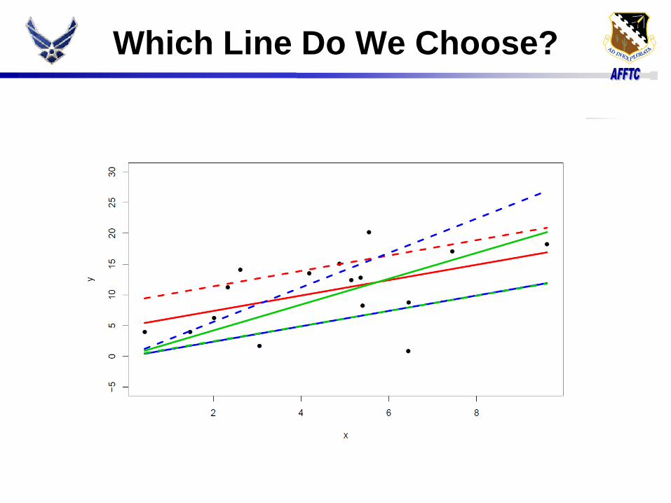
Which Line Do We Choose?

The Line That Minimizes The Errors.

Ramsey, F., Schaffer, D., The Statistical Sleuth, Brooks-Cole, Belmont ,
California, page 180.

Why Do We Fit A Line?
• We then have an estimate of how a
predictor affects the response.
• A formal statistical test also shows
evidence supporting an effect.
• We can predict for values not observed
but within the limits of the data.
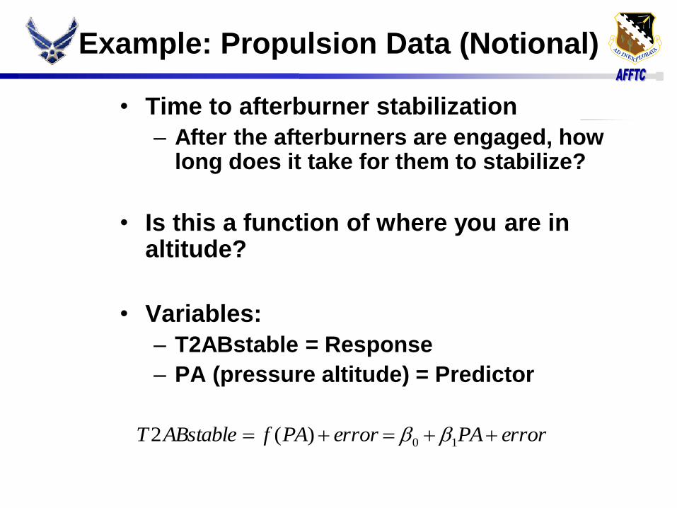
Example: Propulsion Data (Notional)
• Time to afterburner stabilization
– After the afterburners are engaged, how long does it take for them to stabilize?
• Is this a function of where you are in altitude?
• Variables:
– T2ABstable = Response
– PA (pressure altitude) = Predictor
errorPAerrorPAfABstableT 10)(2

Propulsion Regression

Propulsion Regression
• At sea level (intercept) the time to
• stabilization is 5.14 seconds.
• Every unit of pressure altitude after sea level adds 0.00009 seconds to stabilize the afterburner.
• @ Alt = 25,000, T2ABstable = 7.47 sec – I‟m 95% confident that the time to stabilization
will be between 5.65 and 9.28 seconds for future applications of the afterburner.
Estimate Std. Error t value P-value
Intercept 5.13900 0.26510 19.38 < 2e-16
Slope 0.00009 0.00001 10.24 7.08E-14

Model #2
Multiple Linear Regression

Multiple Linear Regression
• An extension of Simple Linear Regression
– Just add more predictors or functions of already used predictors.
• Quadratic, Cubic, and other functions of predictors:
• Interactions
• Additional predictors
• Remember T2ABstable vs. PA…
– Maybe we need more in this model.

Linear vs. Quadratic
Note: this is still linear regression—linear in the
coefficients.
PATABstable 00009.014.5 2910*47.1000018.018.5 PAPATABstable

Is More Complexity Better Here?
• Testing difference of models, we get:
– P-value=0.05692
– General Rule/Philosophy: If p-value < 0.05, then significant.
– Close, but by the 0.05 rule, there is no difference.
– It depends on your own philosophy.

Model #3
GLM - Generalized Linear Models

GLM—Generalized Linear Models
• Suppose we have yes/no (0,1) data for the response.
• Regression finds the mean of the data across X.
• Taking the mean of 0‟s and 1‟s gives us a probability.
– Mean of [0,1,0,0,1] is 0.4, or 40%.
• A link function puts the 0/1 data in a situation where a linear regression can be applied.
Xg 10

Model #3A
Logistic Regression is a GLM
(Logistic Regression is most useful
of GLM‟s)
Logistic Regression

Logistic Regression
• If we fit the regular simple linear
regression we have problems:
– non-normal data,
– and can produce predictions/estimates that
are outside (0,1) interval.
• What is a probability of 1.1, or -0.2?
• What does this look like?

Blip to Scan Ratio: Probability of
Detection
• A radar scans/sweeps an area to detect
objects.
• Blip to Scan Ratio is the ratio of times the
scan detected something to the number of
scans performed.

Blip Scan Fit w/ Linear Regression
(Notional)
Uh Oh! Strange
probabilities… Pr(Blip) >1
Pr(Blip) <0

Blip Scan (Notional)
• For a given slant range, when do we „blip‟:
50% of the time?
80% of the time?
• We use the following link function, the
logit:
)Pr(
1log)(log 10
Blipp
RangeSlantX
Xp
ppit

Logistic Regression—For Probability
of Detect

Model #4
Monte Carlo Methods And
Resampling
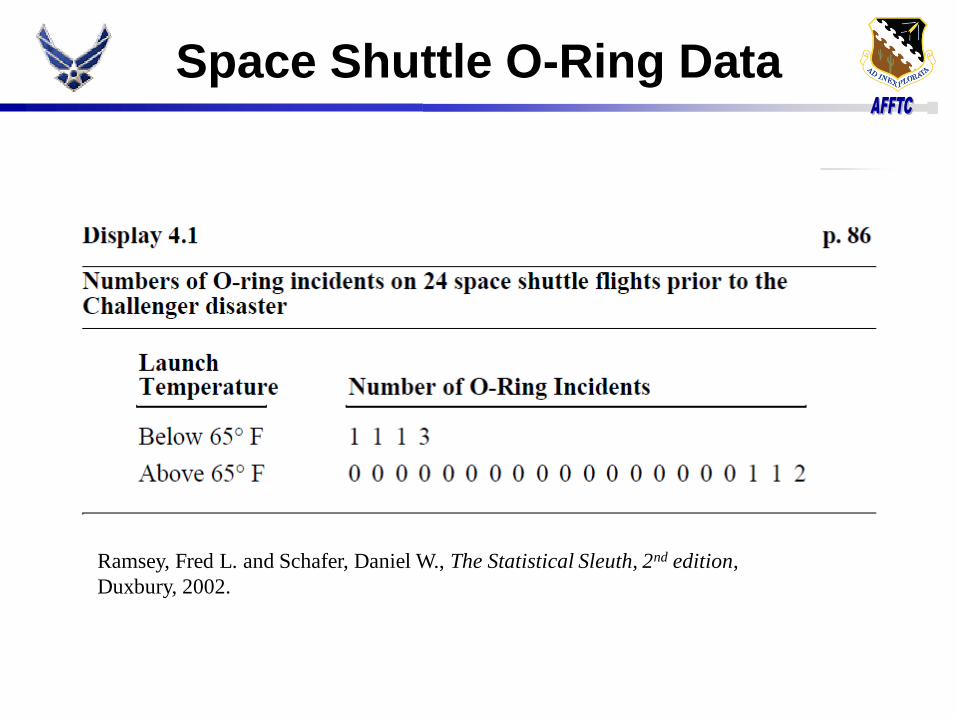
Space Shuttle O-Ring Data
Ramsey, Fred L. and Schafer, Daniel W., The Statistical Sleuth, 2nd edition,
Duxbury, 2002.

The Routine 2 Sample t-test
1. Compute a t-statistic:
wcSE
dwcstatt
Note: If is really equal
to zero, then the t-stat’s
distribution should be Student’s
t distribution.
wc
2. Check to see how likely
this is…
Hypotheses:
H0: μc = μw (OR) d = μc-μw = 0
HA: μc > μw (OR) d = μc-μw > 0
Sometimes this is the
wrong distribution…

Alternate Two Sample Comparison
• IF there is no difference between the two
groups of data,
– Then it wouldn‟t matter if we trade back
and forth between them, the mean for each
group wouldn‟t drastically change.
Compute t-stat Do t-
test…
Can’t, data is not normal, in
more ways than one.
Students t distribution
doesn’t support the t-statistic
anymore. We’ll build our own
distribution using
resampling.

Resampling the O-Ring Data
• Combined O-Ring Data:
– [1 1 1 3 0 0 0 0 0 0 0 0 0 0 0 0 0 0 0 0 0 1 1 2]
• Scramble it up: – [0 0 0 1 0 0 0 1 3 0 0 0 0 1 2 0 1 0 0 1 0 0 0 0]
• Split into two groups: – Cool = [0 0 0 1 ]
– Warm = [0 0 0 1 3 0 0 0 0 1 2 0 1 0 0 1 0 0 0 0]
• If there really isn‟t any difference between the two groups, this re-assignment won‟t matter…

Resampling the O-Ring Data
• Compute the t-statistic for the resampled
set:
o t-stat = -0.4627
• Save this value in a vector.
• Repeat 9,999 times,
o Now we have our custom distribution for
the t-statistic.

Custom Distribution

Outcome
• Compute t-statistic,
– t = 2.5316
– Pr(resampled >= t) = p-value = 0.0033
– If we assume the null (H0) hypothesis is
true, there is a 0.0033 chance that the t
statistic from above could have been
produced.
– The p-value supports the hypothesis that
the cool flights have greater mean number
of incidences.

Other Monte Carlo Methods
• There are vast possibilities with Monte Carlo methods.
• They can range from complex to simple.
• All are helpful in tight spots.
• This provides a whole avenue to follow…Bayesian stats.

1
Statistical Defense
Course #4
May 2011
Air Force Flight Test Center
Arnon Hurwitz & Todd Remund
812 TSS/EN
Edwards AFB, CA 93524
I n t e g r i t y - S e r v i c e - E x c e l l e n c e
Approved for public release; distribution is unlimited. AFFTC-PA No.: PA-10900
War-Winning Capabilities … On Time, On Cost

2
Statistical Defense!
Picture Courtesy of the U.S. Air Force Official Web Site
Screaming Eagle created by Ken Chandler

• Introduction
• Observational Studies and
Experimental Design (DOE)
• Statistical Modeling
Bayesian Techniques
3
Defensible Statistics

Statistically Defensible Analyses-
Part IV: Bayesian
Q. What is the Bayesian Conspiracy? A. The Bayesian Conspiracy is a multinational, interdisciplinary, and shadowy group of statisticians and test engineers who control publication and funding for DT&E, OT&E analyses. The best way to be accepted into the Bayesian Conspiracy is to join the Campus Crusade for Bayes in high school or college, and gradually work your way up to the inner circles. It is rumored that at the upper levels of the Bayesian Conspiracy exist nine silent figures known only as the Bayes Council.
4
Bayesian Statistics In Flight Test,
ITEA, Las Vegas NV, May 2011.

Topics:
• What is Bayesian analysis?
• Why Bayesian analysis
• Bayes vs. Frequentist
• Examples
– discrete: balls in an urn
– continuous (using OpenBUGS): logistic
regression
• Summary: Bayes- the good and the bad
5
Bayesian Statistics In Flight Test,
ITEA, Las Vegas NV, May 2011.

What is “Bayes” Analysis?
• Different approach from frequentist analyses:
– Frequentist:
• throw away any previous information we may have
• estimate a parameter, an unknown constant.
– Bayesian:
• use any previous information we may have
• estimate a distribution for a random variable
• admit hierarchical models
6
Bayesian Statistics In Flight Test,
ITEA, Las Vegas NV, May 2011.
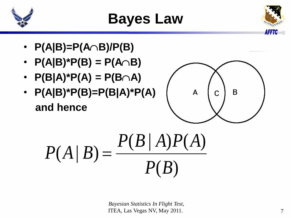
Bayes Law
• P(A|B)=P(AB)/P(B)
• P(A|B)*P(B) = P(AB)
• P(B|A)*P(A) = P(BA)
• P(A|B)*P(B)=P(B|A)*P(A)
and hence
Bayesian Statistics In Flight Test,
ITEA, Las Vegas NV, May 2011.
7
)(
)()|()|(
BP
APABPBAP

Bayes vs. Frequentist
• Frequentist:
– Analysis based on a model
– No prior information
– Estimate an unknown constant (parameter)
– Hypothesis test, p-value, confidence
intervals
– Confidence interval is backwards: 95% CI
doesn’t mean “probability the parameter in
the interval is 0.95. “
8
Bayesian Statistics In Flight Test,
ITEA, Las Vegas NV, May 2011.

Bayes vs. Frequentist
• Bayesian:
– Use hierarchical models
– Estimate a random variable, get a density function
– Incorporate prior information
– Clean interpretation:
• No hypothesis tests, no p-values
• No type I, type II errors-
• Conclusions driven by posterior density
• 95% Credibility Interval means 95% probability the RV is in the interval
9
Bayesian Statistics In Flight Test,
ITEA, Las Vegas NV, May 2011.

Bayes Approach:
– General Bayes Law:
p(θ|x1, x2,…,xk) p(x1, x2,…,xk |θ) * p(θ)
– Θ a vector of RVs- defining the posterior
probability density (Θ = (σx , σy , CEP, CE90
… )T )
– Θ can be a single value, or a vector
10
Bayesian Statistics In Flight Test,
ITEA, Las Vegas NV, May 2011.

Bayes In (4) Easy Steps
• Step 1. Admit you’re a Bayesian. “Hello, my name is Jim, and I’m a Bayesian.”
• Step 2. Atone for all the times you misled clients with a p-value and a confidence interval
– Quick Quiz: the 95% confidence interval for the resistance in ohms of a component is (37.5 , 42.7 )
– T/F I pick a component at random then I’m 95% confident that it will have resistance between 37.5 and 42.7
11
Bayesian Statistics In Flight Test,
ITEA, Las Vegas NV, May 2011.

Resistance in
• FALSE! The resistance either is or is not
in the CI: the probability is either 0 or 1
• The Frequentist CI requires 1000’s of
alternative universes, in each of which a
CI is computed; then the true value is in
95% of all those CI’s. (all different)
• BTW, if you said TRUE, you were thinking
like a Bayesian
Bayesian Statistics In Flight Test,
ITEA, Las Vegas NV, May 2011. 12

Bayes- 4 Easy Steps:
• Step 1: I need a likelihood function; i.e. a
probability density for the x1, x2,…,xk
observations given θ
• Likelihood L(x1, x2,…,xk |θ) = f(x1|θ)f(x2|θ)
… f(xk|θ), pair wise independence of the
xi’s given θ
13
Bayesian Statistics In Flight Test,
ITEA, Las Vegas NV, May 2011.
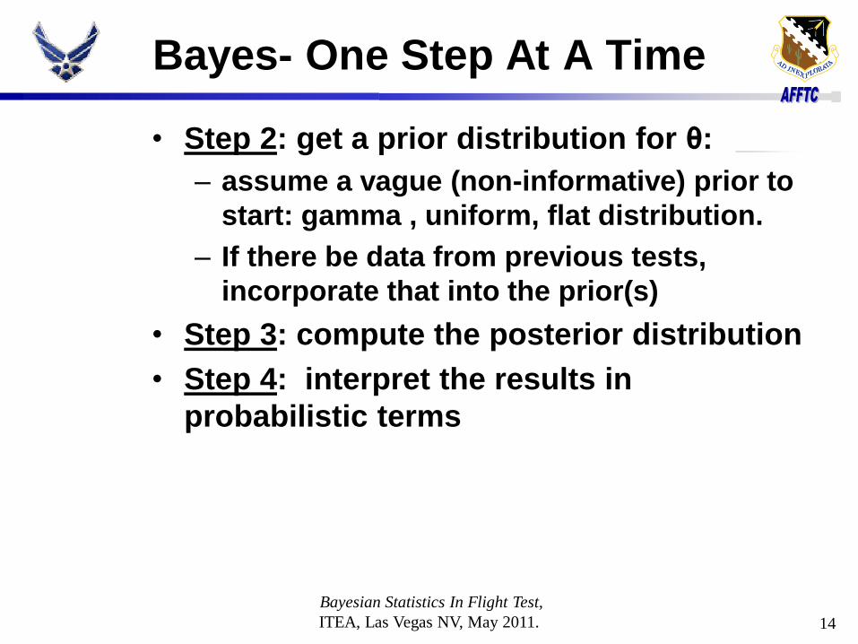
Bayes- One Step At A Time
• Step 2: get a prior distribution for θ:
– assume a vague (non-informative) prior to
start: gamma , uniform, flat distribution.
– If there be data from previous tests,
incorporate that into the prior(s)
• Step 3: compute the posterior distribution
• Step 4: interpret the results in
probabilistic terms
14
Bayesian Statistics In Flight Test,
ITEA, Las Vegas NV, May 2011.

Bayes’ Law
• posterior = likelihood * prior
• p(θ | data) = p(data | θ) * p(θ)
– p(θ | data) ! This is what I want! I.e., what
do I know about θ given the data
• Today’s posterior distribution is
tomorrow’s prior
– Bayes recursion: use the last posterior
distribution as present prior

Discrete Example:
• I have an urn within which there are 12
balls; an unknown number of red balls
and an unknown number of white balls
• I draw a sample of 5 balls from the urn
(without replacement) and observe 2 red
balls. How many red balls are there in the
urn?

Likelihood
• The likelihood of “x” red balls in the
sample, given that there are r red balls in
the urn, and sample size n is:
• Hypergeometric:
n
xn
r
x
r
12
12

Maximum Likelihood Estimate
• If I observe x = 2 red balls in a sample of
size n then the value of “r” that maximizes
Is the maximum likelihood estimator of r.
n
n
rr
12
2
12
2
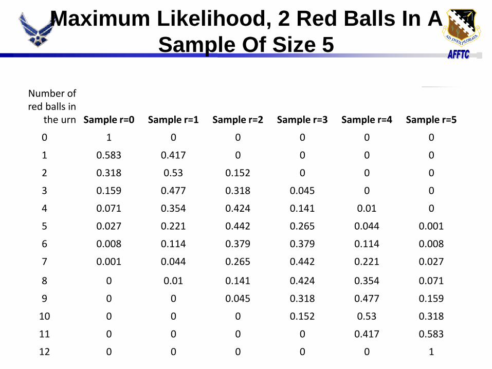
Maximum Likelihood, 2 Red Balls In A
Sample Of Size 5
Number of red balls in
the urn Sample r=0 Sample r=1 Sample r=2 Sample r=3 Sample r=4 Sample r=5
0 1 0 0 0 0 0
1 0.583 0.417 0 0 0 0
2 0.318 0.53 0.152 0 0 0
3 0.159 0.477 0.318 0.045 0 0
4 0.071 0.354 0.424 0.141 0.01 0
5 0.027 0.221 0.442 0.265 0.044 0.001
6 0.008 0.114 0.379 0.379 0.114 0.008
7 0.001 0.044 0.265 0.442 0.221 0.027
8 0 0.01 0.141 0.424 0.354 0.071
9 0 0 0.045 0.318 0.477 0.159
10 0 0 0 0.152 0.53 0.318
11 0 0 0 0 0.417 0.583
12 0 0 0 0 0 1

Likelihood
• So let L(x| n, r) be the likelihood:
n
xn
r
x
r
rnxL12
12
),|(
L(x|n,r)=likelihood of x red balls in the sample, given sample size is n,
and r red balls in the urn

Back To Bays Law- How
About a Prior?
• p(r) = L(x|n,r)*p0(r) = posterior distribution
of the number r of red balls in the urn
• Roll two dice, put r (= sum of the
numbers) red balls in the urn: then p0(r)
(prior probability of r red balls in the urn)
looks like:
r 0 1 2 3 4 5 6 7 8 9 10 11 12
P(r) 0 0 1/
36
2/
36
3/
36
4/
36
5/
36
6/
36
5/
36
4/
36
3/
36
2/
36
1/
36

And Get The Bayesian Estimate
• p(r) = L(2|5,r) * p0(r)
Number of red balls in the urn Prior Likelihood Product Posterior
0 0 0 0 0 1 0 0 0 0 2 0.028 0.152 0.004 0.018 3 0.056 0.318 0.018 0.078 4 0.083 0.424 0.035 0.155 5 0.111 0.442 0.049 0.216 6 0.139 0.379 0.053 0.231 7 0.167 0.265 0.044 0.194 8 0.139 0.141 0.02 0.086 9 0.111 0.045 0.005 0.022
10 0.083 0 0 0 11 0.056 0 0 0 12 0.028 0 0 0

Graphically..
Bayesian Statistics In Flight Test,
ITEA, Las Vegas NV, May 2011. 23
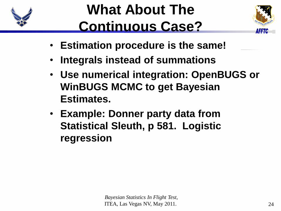
What About The
Continuous Case?
• Estimation procedure is the same!
• Integrals instead of summations
• Use numerical integration: OpenBUGS or
WinBUGS MCMC to get Bayesian
Estimates.
• Example: Donner party data from
Statistical Sleuth, p 581. Logistic
regression
Bayesian Statistics In Flight Test,
ITEA, Las Vegas NV, May 2011. 24

Donner Party Data
Person Sex Age Survival
1 M 23 No
2 F 40 Yes
3 M 40 Yes
4 M 30 No
…
45 F 25 Yes
Bayesian Statistics In Flight Test,
ITEA, Las Vegas NV, May 2011. 25
Logit(p[i]) = alpha + bsex * sex[i] + bage * age[i]
Logit(p[i])defined as: log(p[i]/(1-p[i]), log odds
Estimate alpha, bsex, bage

Logistic Model
• BUGS model for logistic regression:
• log(p[i]/(1-p[i]) = alpha + bsex*sex[i] +
bage*age[i]
• survive[i] ~ dbern(p[i])
• Priors:
– alpha ~ dnorm(0.0, 1.0E-4)
– bsex ~ dnorm(0.0, 1.0E-4)
– bage ~ dnorm(0.0, 1.0E-4)
• Model in R: glm(survival~age+sex, family=binomial)
26
Bayesian Statistics In Flight Test,
ITEA, Las Vegas NV, May 2011.
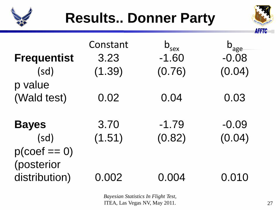
Results.. Donner Party
Constant bsex bage
Frequentist 3.23 -1.60 -0.08 (sd) (1.39) (0.76) (0.04)
p value
(Wald test) 0.02 0.04 0.03
Bayes 3.70 -1.79 -0.09 (sd) (1.51) (0.82) (0.04)
p(coef == 0)
(posterior
distribution) 0.002 0.004 0.010
Bayesian Statistics In Flight Test,
ITEA, Las Vegas NV, May 2011. 27

Bayes And “glm” From R
Bayesian Statistics In Flight Test,
ITEA, Las Vegas NV, May 2011. 28
Red line : GLM
estimate of
coefficient

Conclusions- Bayesian Estimates:
Some Good, Some Bad
• The Good: – Same results as frequentist, but more information,
easier to explain
– Increasingly used: Bayes analysis in epidemiology, medical research, and Bayesian recursive filtering: KEEP UP
– Test efficiency: incorporate data from previous tests: prior distributions, hierarchical models
– Because Bayesian results in a probability distribution • no p-values,
• no hypothesis tests,
• no type I and type II errors,
• no need for thousands of alternative universes to interpret a result
29
Bayesian Statistics In Flight Test,
ITEA, Las Vegas NV, May 2011.

Conclusions- Bayesian Estimations:
Some Good, Some Bad
• The Bad:
– Steep learning curve on R, hierarchical
models and OpenBUGS.
– Numerical aspects of MCMC algorithms:
• Estimating the posterior f(θ| x1, x2,…,xk):
may have convergence problems
• OpenBUGS does not have all distributions,
all mathematical functions: user may have
to supply these
– Issue with priors: what prior to use?
30
Bayesian Statistics In Flight Test,
ITEA, Las Vegas NV, May 2011.
CONGRATULATIONS: You Are Now An
Initiate Of The Bayesian Conspiracy
31
Bayesian Statistics In Flight Test,
ITEA, Las Vegas NV, May 2011.

Post Script..
• Remember: friends don’t let friends
compute p-values.
• Get Help from a Statistician
32
Bayesian Statistics In Flight Test,
ITEA, Las Vegas NV, May 2011.