airborne hyperspectral imaging - fred sigernes

F. Sigernes, Airborne hyperspectral imaging

UNIVERSITY CENTRE ON SVALBARD – P.O.BOX 156 – N 9171 LONGYEARBYEN NORWAY

1

AIRBORNE HYPERSPECTRAL IMAGING F. SIGERNES

1. Introduction The rapid development of imaging detectors, especially the twodimensional silicon Charge Coupled Device (CCD), has resulted in a new generation of imaging spectrographs. In contrast to the use of a photomultiplier tube as detector, the imaging detector provides information on the spatial distribution of the photon intensity along the entrance slit of the spectrograph. The ability of the CCD to image the entrance slit in different wavelengths and intensity has been used to reconstruct the image of the target object with high spectral and spatial resolution.

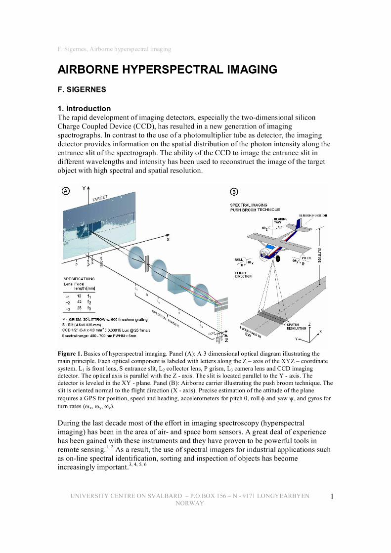
Figure 1. Basics of hyperspectral imaging. Panel (A): A 3 dimensional optical diagram illustrating the main principle. Each optical component is labeled with letters along the Z – axis of the XYZ – coordinate system. L1 is front lens, S entrance slit, L2 collector lens, P grism, L3 camera lens and CCD imaging detector. The optical axis is parallel with the Z axis. The slit is located parallel to the Y axis. The detector is leveled in the XY plane. Panel (B): Airborne carrier illustrating the push broom technique. The slit is oriented normal to the flight direction (X axis). Precise estimation of the attitude of the plane requires a GPS for position, speed and heading, accelerometers for pitch θ, roll φ and yaw ψ, and gyros for turn rates (ωx, ωy, ωz).

During the last decade most of the effort in imaging spectroscopy (hyperspectral imaging) has been in the area of air and space born sensors. A great deal of experience has been gained with these instruments and they have proven to be powerful tools in remote sensing. 1, 2 As a result, the use of spectral imagers for industrial applications such as online spectral identification, sorting and inspection of objects has become increasingly important. 3, 4, 5, 6



2

2. Main principle of hyperspectral imaging In Fig.1 panel (A) shows the optical components of a typical spectrograph. The essential parts are one entrance slit (S), a collector lens (L2), a dispersive element (P) – the grating / prism (grism), a camera lens (L3) and the detector (CCD). The main purpose of a spectrograph is that it generates images of the entrance slit as a function of color. The number of colored slit images on the CCD depends on the width of the entrance slit and the dispersive element’s ability to spread – diffract the colors, and is directly connected to the spectral resolution of the instrument. Focusing light from a target by a front lens (L1) onto the slit plane, forces the instrument to accept structure of the target along the slit. The resulting image (spectrogram) recorded by the CCD is the intensity distribution as a function of wavelength (color) and position along the slit. The spectrogram contains both spectral and spatial information along a thin track of the target object. In our case the target is the ground surface.

Next, in order to obtain the object's full spatial extent, it is necessary to sample the whole object. This requires that the instrument must be moved relative to the target. The whole idea is to record spectrograms for each track of the object as the image at the entrance plane is moved across the slit. Our movement is created by the airplane itself. See Fig.1 panel (B). We are in other word pushing / recording spectrograms as we fly over the ground target. Depending on the application, the relative movement between sensor and target may be obtained by rotating the whole instrument, use of scanning mirrors as front optics, or moving the target itself. The target may for example be located on a conveyor belt or on a sliding table with the sensor mounted to a microscope.

Please note that the use of lenses instead of mirrors is no limitation in implementation of the above idea. The use of a transmitting grating combined with a prism increases the resolution especially in the blue part of the spectrum. In addition, each optical element is aligned along the optical axis (on –axis), reducing geometrical aberrations such as astigmatism and coma. This is the main reason why this type of instrument is one of the most popular designs in the field of hyperspectral imaging. 7

3. Basic imaging spectroscopy In order to calculate both the spectral and spatial resolution of our instrument, it is necessary to look into some basic concepts of spectroscopy. 8

3.1 The modified grating equation As noted above, the spectral resolution depends on the dispersive elements ability to diffract light. Combining a prism and a transmitting grating (grism), requires a two step procedure to calculate the resolution. First light will be diffracted by the grating. Secondly, the prism refracts the light. The light diffracted by the grating is bent back in line by the refracting effect of the prism, or vise versa. A typical grism configuration is shown in Fig. 2.



3

Figure 2. The grating prism (grism). G is grating, P prism, α the incident angle and β the diffracted angle. n is the refractive index.

The grating equation is modified by using Snell’s law

( ) β α λ sin sin + = n a m , [nm] [1]

where m is the spectral order, λ is the wavelength, a the groove spacing, α the incident angle and β the diffracted angle.

n is the refractive index of the prism given by the formula of Cauchy

2 λ B A n + = . [2]

A and B are constants according to substance of the glass material used.

3.2 The dispersion of a grism Angular dispersion is calculated by differentiating equation (1) and (2)

+

=

3

sin 2 cos

λ α

β β λ

B a m

a d d . [nm/degree] [3]

Since dx = f3 dβ then linear dispersion is defined as

=

3

1 f d

d dx d

β λ λ , [nm/mm] [4]

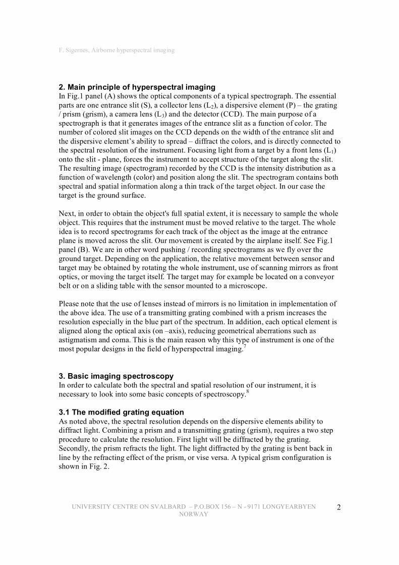
where f3 is the focal length of the camera lens, L3. Linear dispersion gives the spread in wavelength per unit distance in xaxis detector direction. Table 1. shows how the linear dispersion changes with wavelength for our instrument in Fig.1.

It should be noted that the linear dispersion is about 16 nm larger at 400 nm if the prism is removed, using only the grating. Correspondingly, at 800 nm the difference becomes only 4 nm. The grism improves the linear dispersion compared to using only a grating, especially in the blue part of the spectrum. The straight through wavelength of the system is about 480 nm where α = β.



4

Wavelength λ [nm]

Refractive index n

Diffracted angle β [deg.]

Linear dispersion dλ/dx [nm/mm]

300 1.61829 38.9872 37.9174 400 1.58942 33.6908 48.0392 500 1.57606 29.2111 53.9186 600 1.56880 25.1126 57.7198 700 1.56442 21.2360 60.3967 800 1.56158 17.5051 62.3734 900 1.55963 13.8757 63.8542

Table 1. Linear dispersion using a grism with φ = α = 30 o , grating groove spacing a = 1666.667 nm (a 600 lines / mm), spectral order m = 1, and a detector lens with focal length of f3 = 25 mm. Cauchy’s index of refraction constants are A = 1.5523 and B = 5939.39 nm for Borate flint glass.

3.3 Geometrical extent and magnification The geometrical extent (etendue) of the instrument is defined as area of the entrance slit times the effective solid angle that the light propagates into. Or more generally, it is a function of the area, dS, of the emitting source and the solid angle, dQ, into which the light propagates. The etendue at the entrance slit is then

( )

⋅ × = × = 2

2

cos f

G h w dQ dS G A α , [mm 2 sr] [5]

where w and h are the width and height of the entrance slit, respectively. GA cos α is the effective illuminated area of the grism as seen from the entrance slit and f2 is the focal length of lens L2. G characterizes the maximum beam size an instrument can accept, and is a pure geometrical property limited by the size of the different components used. The etendue should be optimized in order to allow light to pass freely through the instrument. The etendue in the exit plane (CCD) is

( )

⋅ ′ × ′ = ′

2 3

cos f

G h w G A β . [mm 2 sr] [6]

An optimal system requires that G G ′ = . Since the grism has no effect on the light in the yaxis direction or along the slit height, magnification or demagnification of the slit height h is only generated by the lenses

h f f

h ×

= ′

2

3 . [mm] [7]

In our case the slit height image is mm h 68 . 2 = ′ . The slit width magnification or demagnification can now be solved from equations (5), (6) and (7)

= ′

2

3

cos cos

f f

w w β α . [mm] [8]



5

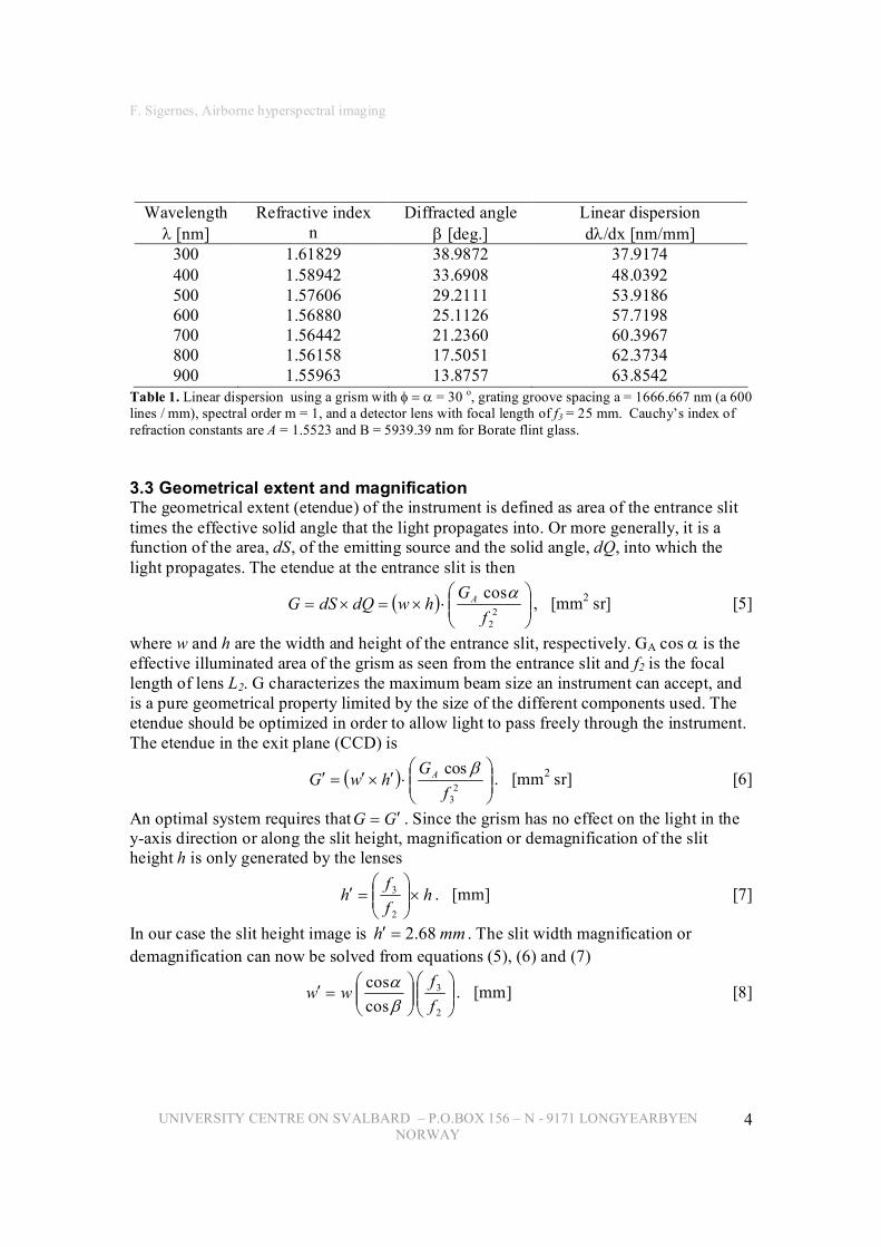
3.4 The instrumental profile and bandpass The instrument’s response to an infinitely narrow monochromatic emission line (real line) with intensity B(λ) will produce a trapezoidal profile F(λ), as a result of a convolution with the instrumental line profile P(λ)

) ( ) ( ) ( λ λ λ P B F ⊗ = . [mW/m 2 nm] [9]

The shape of the P is controlled by the convolution of two rectangular functions with widths equal to the width of the entrance slit image, 1 λ ∆ , and the width of the exit slit

2 λ ∆ , or one pixel in the case of a multichannel detector (CCD), respectively. The natural line width is neglected since it is usually not resolved. We assume no degrade due to aberrations and diffraction effects. The two slit functions are rectangular as illustrated in Fig.3.

Finally, The Full Width at Half Maximum (FWHM) is determined by either the image of the entrance slit or the exit slit, whichever is greater. If the slits are perfectly matched then the line profile will be triangular and the FWHM equals half of the width at the base

Figure 3. The instrumental profile – a convolution of the entrance slits image with the exit slit. The exit slit is in our case just one pixel wide.

of the peak. The spectral bandpass (BP) of the instrument is then calculated as the linear dispersion times the exit slit width

w dx d FWHM BP ′ × ≈ = λ . [nm] [10]

BP is the ability of an instrument to separate adjacent spectral lines. Two emission lines are considered resolved if the distance in wavelength is such that the maximum of one falls on the first minima of the other (Rayleigh criteria). Note that it is normal to allocate at least 3 pixels per bandpass in the detector plane. This number is known as pixels per bin.

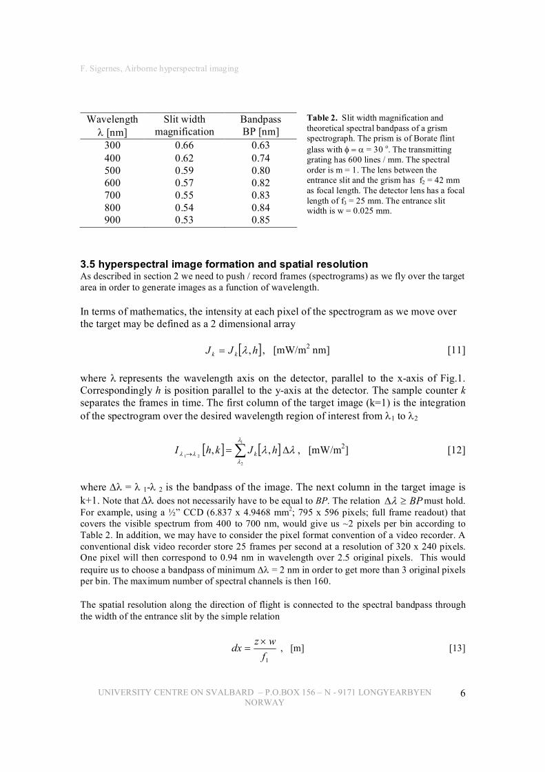
The maximum number of color planes or spectral channels that a hyperspectral imager can produce depends on the spectral bandpass (BP) of the instrument, not the number of pixels along the wavelength axis of the detector (xaxis). Table 2. shows the slit width magnification and the bandpass of our instrument.



6

Wavelength λ [nm]

Slit width magnification

Bandpass BP [nm]

300 0.66 0.63 400 0.62 0.74 500 0.59 0.80 600 0.57 0.82 700 0.55 0.83 800 0.54 0.84 900 0.53 0.85

Table 2. Slit width magnification and theoretical spectral bandpass of a grism spectrograph. The prism is of Borate flint glass with φ = α = 30 o . The transmitting grating has 600 lines / mm. The spectral order is m = 1. The lens between the entrance slit and the grism has f2 = 42 mm as focal length. The detector lens has a focal length of f3 = 25 mm. The entrance slit width is w = 0.025 mm.

3.5 hyperspectral image formation and spatial resolution As described in section 2 we need to push / record frames (spectrograms) as we fly over the target area in order to generate images as a function of wavelength.

In terms of mathematics, the intensity at each pixel of the spectrogram as we move over the target may be defined as a 2 dimensional array

[ ] h J J k k , λ = , [mW/m 2 nm] [11]

where λ represents the wavelength axis on the detector, parallel to the xaxis of Fig.1. Correspondingly h is position parallel to the yaxis at the detector. The sample counter k separates the frames in time. The first column of the target image (k=1) is the integration of the spectrogram over the desired wavelength region of interest from λ1 to λ2

[ ] [ ] λ λ λ

λ λ λ ∆ = ∑ →

1

2

2 1 , , h J k h I k , [mW/m 2 ] [12]

where ∆λ = λ 1λ 2 is the bandpass of the image. The next column in the target image is k+1. Note that ∆λ does not necessarily have to be equal to BP. The relation BP ≥ ∆λ must hold. For example, using a ½” CCD (6.837 x 4.9468 mm 2 ; 795 x 596 pixels; full frame readout) that covers the visible spectrum from 400 to 700 nm, would give us ~2 pixels per bin according to Table 2. In addition, we may have to consider the pixel format convention of a video recorder. A conventional disk video recorder store 25 frames per second at a resolution of 320 x 240 pixels. One pixel will then correspond to 0.94 nm in wavelength over 2.5 original pixels. This would require us to choose a bandpass of minimum ∆λ = 2 nm in order to get more than 3 original pixels per bin. The maximum number of spectral channels is then 160.

The spatial resolution along the direction of flight is connected to the spectral bandpass through the width of the entrance slit by the simple relation

1 f w z dx ×

= , [m] [13]



7

where z is the distance to the target in meters, and f1 is the focal length in millimeters of the front lens L1. Since the plane is moving with velocity v, the spatial resolution is modified as

t v dx x ∆ ⋅ + = ∆ . [m] [14]

The exposure time ∆t of the images does not include the readout time of the detector, τ . The distance moved during readout τ ⋅ v must be less than dx. If not the case, the instrument will miss samples of the target area (under sampling).

Normal to the flight direction the resolution is calculated simply as

N f h z y

× ×

= ∆ 1

, [m] [15]

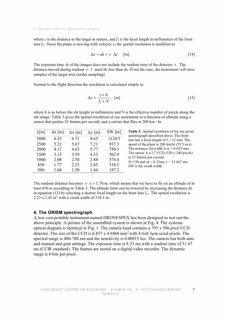
where h is as before the slit height in millimeters and N is the effective number of pixels along the slit image. Table 3 gives the spatial resolution of our instrument as a function of altitude using a sensor that pushes 25 frames per second, and a carrier that flies at 200 km / hr.

z[m] dx [m] ∆x [m] ∆y [m] SW [m] 3000 6.25 6.71 8.65 1124.5 2500 5.21 5.67 7.21 937.3 2000 4.17 4.63 5.77 750.1 1500 3.13 3.59 4.33 562.9 1000 2.08 2.54 2.88 374.4 850 1.77 2.23 2.45 318.5 500 1.04 1.50 1.44 187.2

Table 3. Spatial resolution of for our grism spectrograph described above. The front lens has a focal length of f 1=12 mm. The speed of the plane is 200 km/hr (55.5 m/s). The entrance slit width is w = 0.025 mm. The sensor is a ½” CCD (320 x 240 pixels) at 25 frames per second. N=130 and ∆t = 8.33ms, τ = 31.667 ms. SW is the swath width.

The readout distance becomes 76 . 1 = ⋅τ v m, which means that we have to fly on an altitude of at least 850 m according to Table 3. The altitude limit can be lowered by increasing the distance dx in equation (13) by selecting a shorter focal length on the front lens L1. The spatial resolution is 2.23 x 2.45 m 2 with a swath width of 318.5 m.

4. The GRISM spectrograph A low cost portable instrument named DRONESPEX has been designed to test out the above principle. A picture of the assembled system is shown in Fig. 4. The systems optical diagram is identical to Fig. 1. The camera head contains a 795 x 596 pixel CCD detector. The size of the CCD is 6.837 x 4.9468 mm 2 with 8.6x8.3µm sized pixels. The spectral range is 400700 nm and the sensitivity is 0.00015 lux. The camera has both auto and manual and gain settings. The exposure time is 8.33 ms with a readout time of 31.67 ms (CCIR standard). The frames are stored on a digital video recorder. The dynamic range is 8 bits per pixel.



8

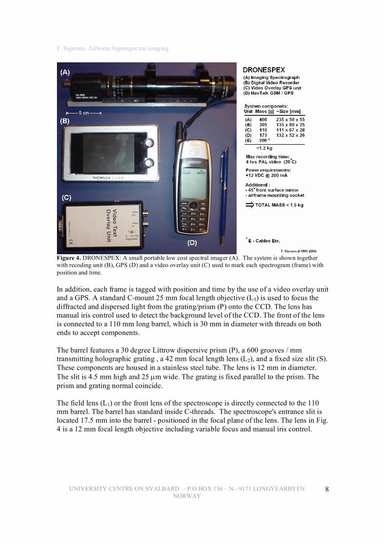
Figure 4. DRONESPEX: A small portable low cost spectral imager (A). The system is shown together with recoding unit (B), GPS (D) and a video overlay unit (C) used to mark each spectrogram (frame) with position and time.

In addition, each frame is tagged with position and time by the use of a video overlay unit and a GPS. A standard Cmount 25 mm focal length objective (L3) is used to focus the diffracted and dispersed light from the grating/prism (P) onto the CCD. The lens has manual iris control used to detect the background level of the CCD. The front of the lens is connected to a 110 mm long barrel, which is 30 mm in diameter with threads on both ends to accept components.

The barrel features a 30 degree Littrow dispersive prism (P), a 600 grooves / mm transmitting holographic grating , a 42 mm focal length lens (L2), and a fixed size slit (S). These components are housed in a stainless steel tube. The lens is 12 mm in diameter. The slit is 4.5 mm high and 25 µm wide. The grating is fixed parallel to the prism. The prism and grating normal coincide.

The field lens (L1) or the front lens of the spectroscope is directly connected to the 110 mm barrel. The barrel has standard inside Cthreads. The spectroscope's entrance slit is located 17.5 mm into the barrel positioned in the focal plane of the lens. The lens in Fig. 4 is a 12 mm focal length objective including variable focus and manual iris control.



9

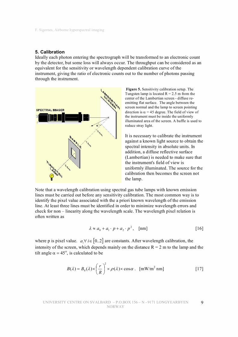
5. Calibration Ideally each photon entering the spectrograph will be transformed to an electronic count by the detector, but some loss will always occur. The throughput can be considered as an equivalent for the sensitivity or wavelength dependent calibration curve of the instrument, giving the ratio of electronic counts out to the number of photons passing through the instrument.

Figure 5. Sensitivity calibration setup. The Tungsten lamp is located R = 2.5 m from the center of the Lambertian screen diffuse re emitting flat surface. The angle between the screen normal and the lamp to screen pointing direction is α = 45 degree. The field of view of the instrument must be inside the uniformly illuminated area of the screen. A baffle is used to reduce stray light.

It is necessary to calibrate the instrument against a known light source to obtain the spectral intensity in absolute units. In addition, a diffuse reflective surface (Lambertian) is needed to make sure that the instrument's field of view is uniformly illuminated. The source for the calibration then becomes the screen not the lamp.

Note that a wavelength calibration using spectral gas tube lamps with known emission lines must be carried out before any sensitivity calibration. The most common way is to identify the pixel value associated with the a priori known wavelength of the emission line. At least three lines must be identified in order to minimize wavelength errors and check for non – linearity along the wavelength scale. The wavelength pixel relation is often written as

2 2 1 0 p a p a a ⋅ + ⋅ + ≈ λ , [nm] [16]

where p is pixel value. [ ] 2 .. 0 ∈ ∀ i a i are constants. After wavelength calibration, the intensity of the screen, which depends mainly on the distance R = 2 m to the lamp and the tilt angle α = 45 ο , is calculated to be

α λ ρ λ λ cos ) ( ) ( ) ( 2

0 × ×

× = R r B B . [mW/m 2 nm] [17]



10

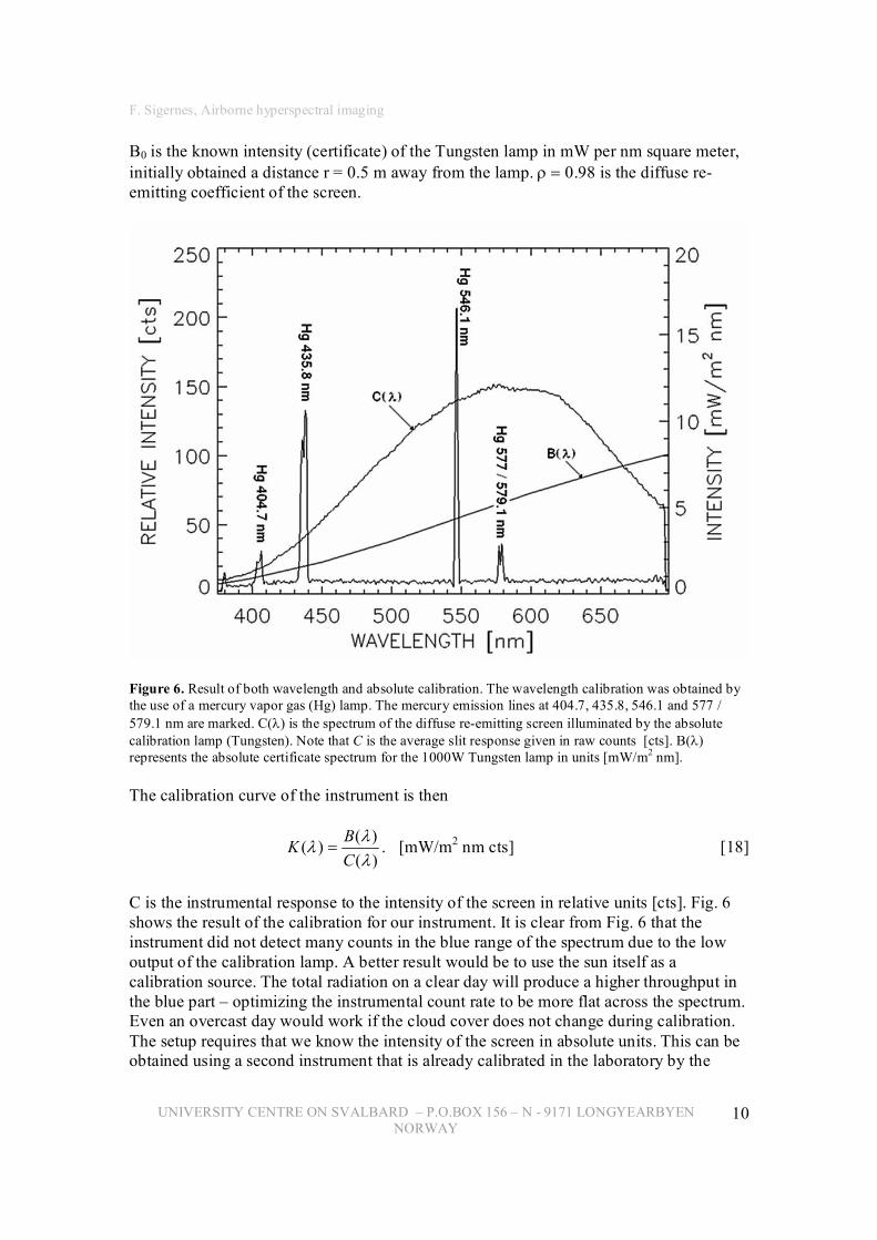
B0 is the known intensity (certificate) of the Tungsten lamp in mW per nm square meter, initially obtained a distance r = 0.5 m away from the lamp. ρ = 0.98 is the diffuse re emitting coefficient of the screen.

Figure 6. Result of both wavelength and absolute calibration. The wavelength calibration was obtained by the use of a mercury vapor gas (Hg) lamp. The mercury emission lines at 404.7, 435.8, 546.1 and 577 / 579.1 nm are marked. C(λ) is the spectrum of the diffuse reemitting screen illuminated by the absolute calibration lamp (Tungsten). Note that C is the average slit response given in raw counts [cts]. B(λ) represents the absolute certificate spectrum for the 1000W Tungsten lamp in units [mW/m 2 nm].

The calibration curve of the instrument is then

) ( ) ( ) (

λ λ λ

C B K = . [mW/m 2 nm cts] [18]

C is the instrumental response to the intensity of the screen in relative units [cts]. Fig. 6 shows the result of the calibration for our instrument. It is clear from Fig. 6 that the instrument did not detect many counts in the blue range of the spectrum due to the low output of the calibration lamp. A better result would be to use the sun itself as a calibration source. The total radiation on a clear day will produce a higher throughput in the blue part – optimizing the instrumental count rate to be more flat across the spectrum. Even an overcast day would work if the cloud cover does not change during calibration. The setup requires that we know the intensity of the screen in absolute units. This can be obtained using a second instrument that is already calibrated in the laboratory by the



11

procedure outlined above. The second instrument does not need to have imaging or hyperspectral capability – a regular spectrograph with a line array detector sensitive in the blue will be sufficient.

6. Example applications A whole range of possible applications can be investigated using hyperspectral imaging. Each spectral image represents how effectively a target scene absorbs, reflects or scatters light at the selected centre wavelength. A set of spectral images will produce a unique spectral finger print for each object within a target scene. This type of data becomes ideal as input for sorting of objects by the use of image processing algorithms like classification. 9

Data from our airborne campaigns in the arctic cover application such as mapping of

1. Ocean colour and algae’s 2. Vegetation and rocks 3. Sea ice and leads 4. Snow cover.

In the following examples, a commercial twin engine aeroplane of type Dornier228, operated by the company Lufttransport AS with base in Longyearbyen, Svalbard (78 o N, 15 o E), has been used as carrier of the instruments. The pointing direction of the imagers is 30 degrees to nadir (side view). For each mission a sliding door has been mounted on the plane, which can be opened during flight when approaching the target area. Position and speed is obtained by using the external GPS antenna of the plane. The attitude (pitch, roll and yaw) is estimated by using realtime data from 3 axis accelerometers and electronic turn rate sensors. A Kalman estimator is used to process the attitude data.

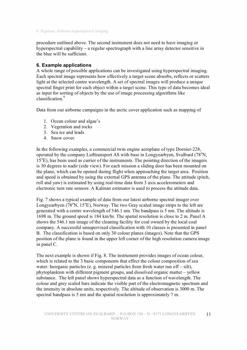
Fig. 7 shows a typical example of data from our latest airborne spectral imager over Longyearbyen (78 o N, 15 o E), Norway. The two Gray scaled image strips to the left are generated with a centre wavelength of 546.1 nm. The bandpass is 5 nm. The altitude is 1698 m. The ground speed is 184 km/hr. The spatial resolution is close to 2 m. Panel A shows the 546.1 nm image of the cleaning facility for coal owned by the local coal company. A successful unsupervised classification with 10 classes is presented in panel B. The classification is based on only 30 colour planes (images). Note that the GPS position of the plane is found in the upper left corner of the high resolution camera image in panel C.

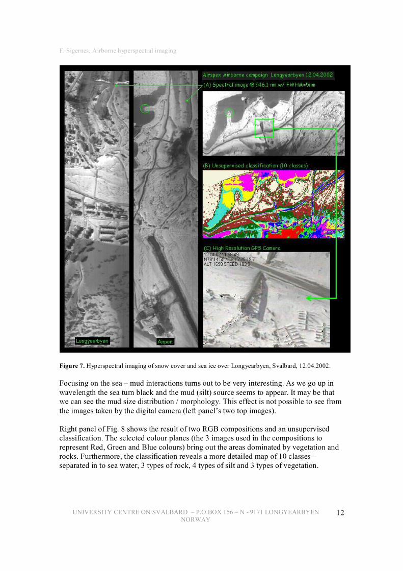
The next example is shown if Fig. 8. The instrument provides images of ocean colour, which is related to the 3 basic components that effect the colour composition of sea water: Inorganic particles (e. g. mineral particles from fresh water run off – silt), phytoplankton with different pigment groups, and dissolved organic matter – yellow substance. The left panel shows hyperspectral data as a function of wavelength. The colour and grey scaled bars indicate the visible part of the electromagnetic spectrum and the intensity in absolute units, respectively. The altitude of observation is 3000 m. The spectral bandpass is 5 nm and the spatial resolution is approximately 7 m.



12

Figure 7. Hyperspectral imaging of snow cover and sea ice over Longyearbyen, Svalbard, 12.04.2002.

Focusing on the sea – mud interactions turns out to be very interesting. As we go up in wavelength the sea turn black and the mud (silt) source seems to appear. It may be that we can see the mud size distribution / morphology. This effect is not possible to see from the images taken by the digital camera (left panel’s two top images).

Right panel of Fig. 8 shows the result of two RGB compositions and an unsupervised classification. The selected colour planes (the 3 images used in the compositions to represent Red, Green and Blue colours) bring out the areas dominated by vegetation and rocks. Furthermore, the classification reveals a more detailed map of 10 classes – separated in to sea water, 3 types of rock, 4 types of silt and 3 types of vegetation.



13

Figure 8. Hyperspectral imaging of ocean colour, vegetation and rocks over the bays of Collinderodden and Blixodden close to the mining town of Svea, Svalbard, 25.07.2000.

Note that a supervised classification would improve and optimize the above results, but that requires insitu observations on the ground. In many cases this can prove to be difficult due to logistics and access to the target area. Nevertheless, it is clearly evident that it is indeed necessary to combine insitu observations to support and understand the airborne data better.



14

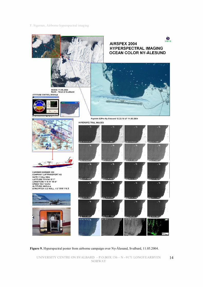
Figure 9. Hyperspectral poster from airborne campaign over NyÅlesund, Svalbard, 11.05.2004.



15

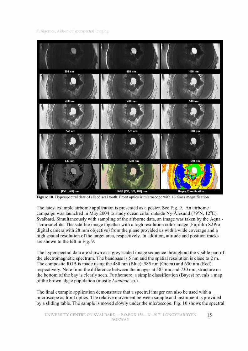
Figure 10. Hyperspectral data of sliced seal tooth. Front optics is microscope with 16 times magnification.

The latest example airborne application is presented as a poster. See Fig. 9. An airborne campaign was launched in May 2004 to study ocean color outside NyÅlesund (79 o N, 12 o E), Svalbard. Simultaneously with sampling of the airborne data, an image was taken by the Aqua Terra satellite. The satellite image together with a high resolution color image (Fujifilm S2Pro digital camera with 28 mm objective) from the plane provided us with a wide coverage and a high spatial resolution of the target area, respectively. In addition, attitude and position tracks are shown to the left in Fig. 9.

The hyperspectral data are shown as a grey scaled image sequence throughout the visible part of the electromagnetic spectrum. The bandpass is 5 nm and the spatial resolution is close to 2 m. The composite RGB is made using the 480 nm (Blue), 585 nm (Green) and 630 nm (Red), respectively. Note from the difference between the images at 585 nm and 730 nm, structure on the bottom of the bay is clearly seen. Furthemore, a simple classification (Bayes) reveals a map of the brown algae population (mostly Laminae sp.).

The final example application demonstrates that a spectral imager can also be used with a microscope as front optics. The relative movement between sample and instrument is provided by a sliding table. The sample is moved slowly under the microscope. Fig. 10 shows the spectral



16

images from 390 to 690 nm of a sliced seal to. The bandpass of the images is 15 nm. The slice is 1 mm thick. The magnification was set to 16 times on the microscope. The light source is located under the sample light is transmitted through the sliced tooth. A processed image showing the difference between the 450 and 570 nm images reveals structure, and a composite RGB shows the colour image. Classification sorts out 8 different classes. Note that there is a small mix or miss classification. This is mainly due to cracks in the tooth and that the sample itself is glued to the sample glass (seen as a transparent area in the centre of the images). Nevertheless, the age rings of the tooth are clearly identified with the colour red. The seal was two years old.

7. Future remark on hyperspectral imaging Optics is one of the oldest branches of physics. Spectroscopy started when Newton decided to celebrate the colors of life with a prism back in the late 1700. Even today optics is one of the fastest growing fields of physics, and is extending its use to other branches of science. The advances in electronics and new materials have resulted in detectors that are able to sense light outside the visible part of the spectrum. The recent development of Acoustic Optical Tunable Filters (AOTF) will revolutionize spectroscopy just as the arrival of blazed gratings did back in the 50’s. UV imagers and near to far infrared imagers will soon be available even on the commercial market to a reasonable price. These spectral imagers will open our eyes to things we have never seen before.

References 1. G. Vane, ed., Imaging Spectroscopy II, Proc. SPIE 834 (1988).

2. W.L. Wolfe, Introduction to Imaging Spectrometers, Vol. TT25 of Tutorial Text Series (SPIE Press, Bellingham, Wash., 1997), pp. 1147.

3. E. Herrala, and J. Okkonen, Imaging spectrograph and camera solutions for industrial applications, International Journal of Pattern Recognition and Artificial Intelligence, 10 (1), 4354, 1996.

4. T. Hyvarinen, E. Herrala, and A. Dall'Ava, Direct sight imaging spectrograph: a unique addon component brings spectral imaging to industrial applications, (SPIE Symposium on Electronic Imaging, Paper 330221, San Jose, California, January 2530, 1998).

5. F. Sigernes, K. Heia, H. Nilsen, and T. Svenøe, Imaging spectroscopy applied in the fish industry?, Norwegian Society for Image Processing and Pattern Recognition, 2, 16 24, 1998.

6. Nilsen, H., Esaiassen, M., Karsten, H., and Sigernes, F., VIS/NIR spectroscopy a new tool for the evaluation of fish freshness?, Journal of Food Science, 67, No. 5, 1821 1826, 2002.



17

7. Sigernes, F., Lorentzen, D.A., Heia, K., and Svenøe, T., A multipurpose spectral imager, 39, N0.18, 3143, (front cover issue), Applied Optics, 2000.

8. C. Palmer, Diffraction Gratings Handbook, 5 th ed. Thermo RGL (Richardson Grating Laboratory, 2002), pp. 142 – 144.

9. W. Niblack, An Introduction to digital image processing, Vol. 1 (Prentice / Hall international (UK) Ltd., 1986), pp. 168181.

airborne hyperspectral imaging - fred sigernes

Documents