UNIT 5.8 POLYNOMIAL UNIT 5.8 POLYNOMIAL MODELS IN THE REAL WORLDMODELS IN THE REAL WORLD

Warm UpFind a line of best fit for the data.

y = 5.45x + 36.12

1.

2.

y = –1.28x + 132.66

x 2 8 15 21 24

y 70 62 80 190 160

x 38 42 44 35 49

y 92 80 75 81 68

Use finite differences to determine the degree of a polynomial that will fit a given set of data.

Use technology to find polynomial models for a given set of data.

Objectives

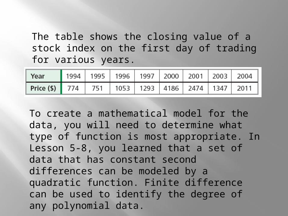
The table shows the closing value of a stock index on the first day of trading for various years.

To create a mathematical model for the data, you will need to determine what type of function is most appropriate. In Lesson 5-8, you learned that a set of data that has constant second differences can be modeled by a quadratic function. Finite difference can be used to identify the degree of any polynomial data.

Use finite differences to determine the degree of the polynomial that best describes the data.

Example 1A: Using Finite Differences to Determine Degree

The x-values increase by a constant 2. Find the differences of the y-values.

x 4 6 8 10 12 14

y –2 4.3 8.3 10.5 11.4 11.5

y –2 4.3 8.3 10.5 11.4 11.5

First differences: 6.3 4 2.2 0.9 0.1 Not constant Second differences: –2.3 –1.8 –1.3 –0.8 Not constant

The third differences are constant. A cubic polynomial best describes the data.

Third differences: 0.5 0.5 0.5 Constant

Use finite differences to determine the degree of the polynomial that best describes the data.

Example 1B: Using Finite Differences to Determine Degree

The x-values increase by a constant 3. Find the differences of the y-values.

x –6 –3 0 3 6 9

y –9 16 26 41 78 151

y –9 16 26 41 78 151

First differences: 25 10 15 37 73 Not constant Second differences: –15 5 22 36 Not constant

The fourth differences are constant. A quartic polynomial best describes the data.

Third differences: 20 17 14 Not constant Fourth differences: –3 –3 Constant

Check It Out! Example 1

Use finite differences to determine the degree of the polynomial that best describes the data.

The x-values increase by a constant 3. Find the differences of the y-values.

x 12 15 18 21 24 27

y 3 23 29 29 31 43

y 3 23 29 29 31 43

Second differences: –14 –6 2 10 Not constant

The third differences are constant. A cubic polynomial best describes the data.

Third differences: 8 8 8 Constant

First differences: 20 6 0 2 12 Not constant

Once you have determined the degree of the polynomial that best describes the data, you can use your calculator to create the function.

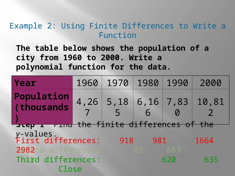
Example 2: Using Finite Differences to Write a Function

The table below shows the population of a city from 1960 to 2000. Write a polynomial function for the data.

Step 1 Find the finite differences of the y-values.

Year 1960 1970 1980 1990 2000

Population (thousands)

4,267 5,185 6,166 7,830 10,812

Second differences: 63 683 1318 Third differences: 620 635 Close

First differences: 918 981 1664 2982

Example 2 Continued

Step 2 Determine the degree of the polynomial.

Because the third differences are relatively close, a cubic function should be a good model.

Step 3 Use the cubic regression feature on your calculator.

f(x) ≈ 0.10x3 – 2.84x2 + 109.84x + 4266.79

Check It Out! Example 2

The table below shows the gas consumption of a compact car driven a constant distance at various speed. Write a polynomial function for the data.

Step 1 Find the finite differences of the y-values.

Speed 25 30 35 40 45 50 55 60

Gas (gal) 23.8 25 25.2 25 25.4 27 30.6 37

Second differences: –1 –0.4 0.6 1.2 2 2.8Third differences: 0.6 1 0.6 0.8 0.8Close

First differences: 1.2 0.2 –0.2 0.4 1.6 3.6 6.4

Check It Out! Example 2 Continued

Step 2 Determine the degree of the polynomial.

Because the third differences are relatively close, a cubic function should be a good model.

Step 3 Use the cubic regression feature on your calculator.

f(x) ≈ 0.001x3 – 0.113x2 + 4.134x + 24.867

Often, real-world data can be too irregular for you to use finite differences or find a polynomial function that fits perfectly. In these situations, you can use the regression feature of your graphing calculator. Remember that the closer the R2-value is to 1, the better the function fits the data.

Example 3: Curve Fitting Polynomial ModelsThe table below shows the opening value of a stock index on the first day of trading in various years. Use a polynomial model to estimate the value on the first day of trading in 2000.

Step 1 Choose the degree of the polynomial model.Let x represent the number of years since 1994. Make a scatter plot of the data.The function appears to be cubic or quartic. Use the regression feature to check the R2-values.

Year 1994 1995 1996 1997 1998 1999

Price ($) 683 652 948 1306 863 901

cubic: R2 ≈ 0.5833 quartic: R2 ≈ 0.8921The quartic function is more appropriate choice.

Step 2 Write the polynomial model. The data can be modeled by f(x) = 32.23x4 – 339.13x3 + 1069.59x2 – 858.99x + 693.88

Step 3 Find the value of the model corresponding to 2000.

2000 is 6 years after 1994. Substitute 6 for x in the quartic model.

Example 3 Continued

f(6) = 32.23(6)4 – 339.13(6)3 + 1069.59(6)2 – 858.99(6) + 693.88

Based on the model, the opening value was about $2563.18 in 2000.

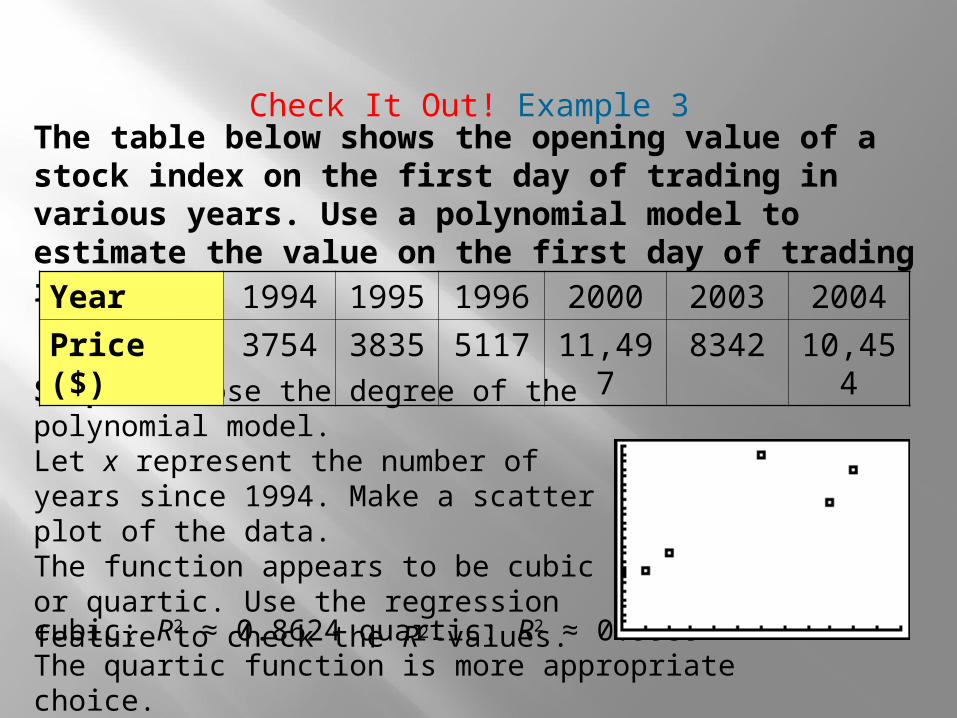
Check It Out! Example 3 The table below shows the opening value of a stock index on the first day of trading in various years. Use a polynomial model to estimate the value on the first day of trading in 1999.

Step 1 Choose the degree of the polynomial model.Let x represent the number of years since 1994. Make a scatter plot of the data.The function appears to be cubic or quartic. Use the regression feature to check the R2-values.

Year 1994 1995 1996 2000 2003 2004

Price ($) 3754 3835 5117 11,497 8342 10,454

cubic: R2 ≈ 0.8624 quartic: R2 ≈ 0.9959The quartic function is more appropriate choice.

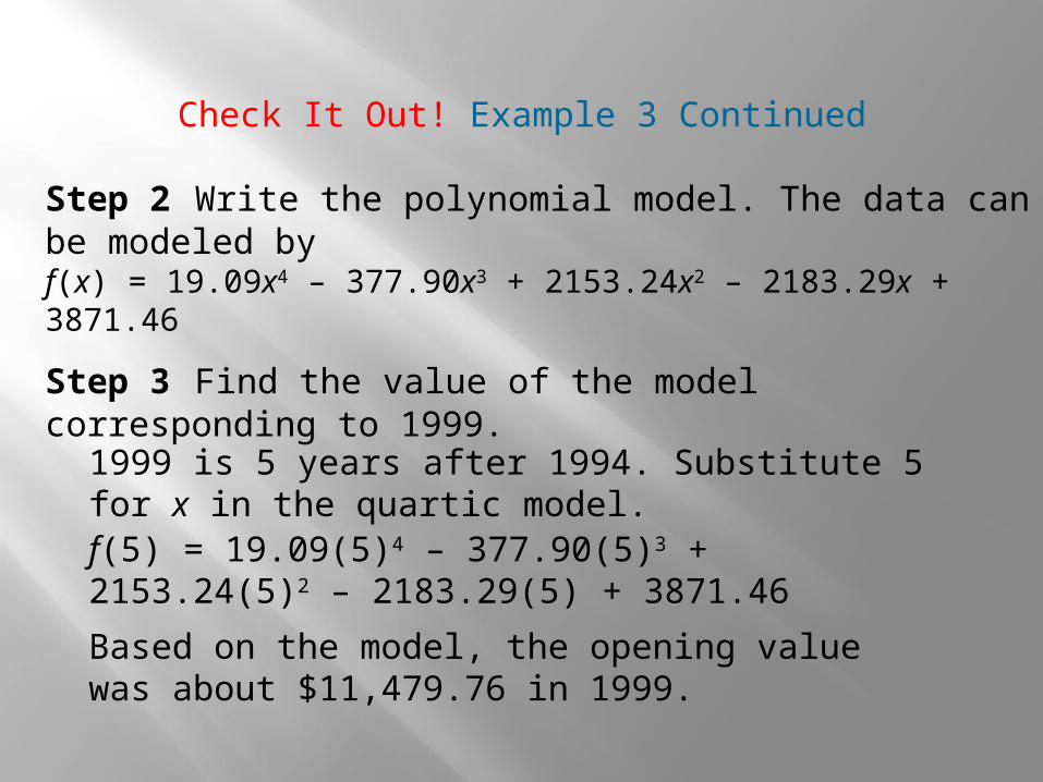
Check It Out! Example 3 Continued

Step 2 Write the polynomial model. The data can be modeled by f(x) = 19.09x4 – 377.90x3 + 2153.24x2 – 2183.29x + 3871.46

Step 3 Find the value of the model corresponding to 1999.

1999 is 5 years after 1994. Substitute 5 for x in the quartic model. f(5) = 19.09(5)4 – 377.90(5)3 + 2153.24(5)2 – 2183.29(5) + 3871.46

Based on the model, the opening value was about $11,479.76 in 1999.

Lesson Quiz: Part I

1. Use finite differences to determine the degree of the polynomial that best describes the data.

cubic

x 8 10 12 14 16 18

y 7.2 1.2 –8.3 –19.1 –29 –35.8

2.

Lesson Quiz: Part II

f(x) = 7.08x4 – 126.92x3 + 595.95x2 – 241.81x + 2780.54; about $3003.50

The table shows the opening value of a stock index on the first day of trading in various years. Write a polynomial model for the data and use the model to estimate the value on the first day of trading in 2002.

Year 1994 1996 1998 2000 2001 2004

Price ($) 2814 3603 5429 3962 4117 3840

All rights belong to their respective owners.Copyright Disclaimer Under Section 107 of the Copyright Act 1976, allowance is made for "fair use" for purposes such as criticism,

comment, news reporting, TEACHING, scholarship, and research.

Fair use is a use permitted by copyright statute that might otherwise be infringing.

Non-profit, EDUCATIONAL or personal use tips the balance in favor of fair use.