algebraic topology - florida atlantic universitymath.fau.edu/yiu/algebraic topology 2006.pdf ·...
TRANSCRIPT
Algebraic Topology
Paul Yiu
Department of MathematicsFlorida Atlantic University
Summer 2006
Wednesday, June 7, 2006
Monday 5/15 5/22 *** 6/5 6/12 6/19Wednesday 5/17 5/24 5/31 6/7 6/14 6/21Friday 5/19 5/26 6/2 6/9 6/16 6/23

Contents
1 General topology 1011.1 Separation axioms . . . . . . . . . . . . . . . . . . . . 1021.2 Compactness . . . . . . . . . . . . . . . . . . . . . . . 1021.3 Connectedness and path-connectedness . . . . . . . . . 1031.4 Compact-open topology on function spaces . . . . . . . 103
2 Homeomorphism 1052.1 Homeomorphism . . . . . . . . . . . . . . . . . . . . 1052.2 The unit cube, unit disk, and standard n-simplex . . . . 1062.3 The sphere S
n . . . . . . . . . . . . . . . . . . . . . . 1072.3.1 Stereographic projection . . . . . . . . . . . . . 108
3 Quotient topology and one-point compactification 1093.1 Quotient space . . . . . . . . . . . . . . . . . . . . . . 1093.2 The projective spaces . . . . . . . . . . . . . . . . . . 109
3.2.1 Complex projective spaces . . . . . . . . . . . . 1103.3 Collapsing a closed subspace . . . . . . . . . . . . . . 1103.4 One-point compactification . . . . . . . . . . . . . . . 110
4 Homotopy 2014.1 Homotopy equivalence . . . . . . . . . . . . . . . . . 2024.2 Nullhomotopy of S
m −→ Sn for m < n . . . . . . . . 203
5 Homotopy functors and their applications 2055.1 Categories and functors . . . . . . . . . . . . . . . . . 205
5.1.1 Covariant and contravariant functors . . . . . . . 2055.2 An example: Brouwer’s fixed point theorem . . . . . . 206
iv CONTENTS
6 Euclidean spaces and their linear maps 2096.1 Linear maps on euclidean spaces . . . . . . . . . . . . 210
6.1.1 The matrix of a linear map . . . . . . . . . . . . 2106.1.2 The adjoint of a linear map . . . . . . . . . . . . 2106.1.3 Determinant . . . . . . . . . . . . . . . . . . . . 211
6.2 The spectral theorem on self-adjoint linear maps . . . . 2116.3 Isometries of Rn . . . . . . . . . . . . . . . . . . . . . 2126.4 The orthogonal groups . . . . . . . . . . . . . . . . . . 212
6.4.1 The hyperplane reflection map . . . . . . . . . . 213
7 The quaternions and the octonions 3017.1 The quaternions . . . . . . . . . . . . . . . . . . . . . 3017.2 The octonions . . . . . . . . . . . . . . . . . . . . . . 3027.3 The Cayley-Dickson algebras . . . . . . . . . . . . . . 303
7.3.1 Commutators and associators in Cayley-Dicksonalgebras . . . . . . . . . . . . . . . . . . . . . . 304
7.4 Appendix: zero divisors in A4 . . . . . . . . . . . . . . 305
8 Quaternions and isometries in R4 307
9 Normed bilinear maps and their Hopf constructions 3099.1 Hurwitz’s theorem . . . . . . . . . . . . . . . . . . . . 3099.2 Normed bilinear maps and Hopf construction . . . . . . 310
9.2.1 The classical Hopf maps . . . . . . . . . . . . . 3109.2.2 Tabulation of a bilinear map . . . . . . . . . . . 3119.2.3 A normed bilinear map R10 × R10 −→ R16 . . . 311
9.3 Appendix: Hurwitz-Radon theorem and the normed bi-linear map problem . . . . . . . . . . . . . . . . . . . 312
10 Polynomial maps between spheres 40110.1 Wood’s theorem . . . . . . . . . . . . . . . . . . . . . 401
10.1.1 Proof of Wood’s theorem: homogeneous case . . 40110.1.2 Proof of Wood’s theorem: general case . . . . . 403
10.2 Appendix: Pfister’s theorem . . . . . . . . . . . . . . . 403
11 Nonsingular bilinear maps 40511.1 Nonsingular bilinear maps on euclidean spaces . . . . . 405
11.1.1 Imbedding of real projective spaces . . . . . . . 40611.1.2 Hopf-Stiefel theorem . . . . . . . . . . . . . . . 40611.1.3 A nonsingular bilinear map R
16 × R16 −→ R23 . 407
CONTENTS v
11.2 The Hopf construction of a nonsingular bilinear map . . 407
12 Quadratic forms between euclidean spheres 40912.1 Quadratic forms between euclidean spaces . . . . . . . 40912.2 Quadratic forms between euclidean spheres . . . . . . . 40912.3 Hidden normed bilinear maps . . . . . . . . . . . . . . 41012.4 The hidden normed bilinear maps of a monomial bilin-
ear map . . . . . . . . . . . . . . . . . . . . . . . . . . 41312.5 Appendix: An application . . . . . . . . . . . . . . . . 413
13 Spaces of similarities 50113.1 The space Hom(Rs,Rn) of linear maps . . . . . . . . . 501
13.1.1 Similarities . . . . . . . . . . . . . . . . . . . . 50113.2 Spaces of similarities and normed bilinear maps . . . . 502
14 Isoclinic n-planes in R2n 50314.1 Angles between two n-planes in R2n . . . . . . . . . . 50314.2 Maximal sets of isoclinic n-planes in R2n . . . . . . . . 504
15 Hurwitz-Radon Theorem 50515.1 Normed bilinear maps and systems of anticommuting
skew symmetric matrices . . . . . . . . . . . . . . . . 50515.2 (r, s)-families of similarities . . . . . . . . . . . . . . . 506
15.2.1 Proof of subspace lemma . . . . . . . . . . . . . 50715.2.2 Proof of shift and expansion lemmas . . . . . . . 50815.2.3 Proof of shift lemma . . . . . . . . . . . . . . . 50815.2.4 Proof of expansion lemma . . . . . . . . . . . . 50915.2.5 Proof of reduction lemma . . . . . . . . . . . . 51015.2.6 Proof of upper bound theorem . . . . . . . . . . 510
15.3 Hurwitz-Radon theorem . . . . . . . . . . . . . . . . . 511
16 Fundamental group 60116.1 The loop space Ω(X, x0) and the fundamental group
π1(X, x0) . . . . . . . . . . . . . . . . . . . . . . . . . 60116.1.1 Conjugacy of fundamental groups . . . . . . . . 603
16.2 The fundamental group of the circle . . . . . . . . . . . 60416.3 Fundamental theorem of algebra . . . . . . . . . . . . 605
vi CONTENTS
17 Covering spaces 60717.1 Covering maps . . . . . . . . . . . . . . . . . . . . . . 60717.2 Covering spaces and fundamental groups . . . . . . . . 60817.3 Universal covering . . . . . . . . . . . . . . . . . . . . 60917.4 Borsuk-Ulam theorem for S2 . . . . . . . . . . . . . . 610
18 Calculation of fundamental groups 61118.1 Van Kampen theorem . . . . . . . . . . . . . . . . . . 61118.2 Fundamental group from triangulations . . . . . . . . . 612
19 Group structures on [X, Y ] 70119.1 Topological groups . . . . . . . . . . . . . . . . . . . 70119.2 H-spaces . . . . . . . . . . . . . . . . . . . . . . . . . 701
19.2.1 The space of loops . . . . . . . . . . . . . . . . 70419.3 Co-H-spaces and suspensions . . . . . . . . . . . . . . 704
19.3.1 The reduced suspension . . . . . . . . . . . . . 70519.4 Homotopy groups . . . . . . . . . . . . . . . . . . . . 707
20 The homotopy groups 70920.1 Higher homotopy groups . . . . . . . . . . . . . . . . 70920.2 Relative homotopy groups . . . . . . . . . . . . . . . . 71020.3 Alternative description of homotopy groups . . . . . . 71020.4 The homotopy exact sequence of a pair . . . . . . . . . 71120.5 Appendix: calculations with exact sequences . . . . . . 713
21 Homotopy exact sequence 71521.1 Locally trivial bundles . . . . . . . . . . . . . . . . . . 71521.2 Homotopy exact sequence of a locally trivial bundle . . 71621.3 Applications of the homotopy exact sequence . . . . . 716
21.3.1 πn(S1) = 0 for n > 1 . . . . . . . . . . . . . . . 716
21.3.2 πm(RPn) ≈ πm(Sn) for m ≥ 2 . . . . . . . . . 716
22 Some homotopy groups of spheres 71722.1 Stable homotopy groups of spheres . . . . . . . . . . . 71722.2 The 0-stem . . . . . . . . . . . . . . . . . . . . . . . . 71722.3 π3(S
2) = Z . . . . . . . . . . . . . . . . . . . . . . . . 718
23 Smooth manifolds 80123.1 Smooth maps . . . . . . . . . . . . . . . . . . . . . . 80123.2 Smooth manifolds . . . . . . . . . . . . . . . . . . . . 801
CONTENTS vii
23.3 Examples of smooth manifolds . . . . . . . . . . . . . 80223.3.1 Smooth connected 1-manifolds . . . . . . . . . . 80223.3.2 The sphere . . . . . . . . . . . . . . . . . . . . 80223.3.3 The real projective spaces . . . . . . . . . . . . 80223.3.4 The Grassman manifolds . . . . . . . . . . . . . 80323.3.5 Spaces of matrices of constant rank . . . . . . . 803
23.4 Appendix: Milnor’s proof of the fundamental theoremof algebra . . . . . . . . . . . . . . . . . . . . . . . . 804
24 Mappings between manifolds 80524.1 Tangent space . . . . . . . . . . . . . . . . . . . . . . 80524.2 Approximation of continuous map by a smooth one . . 80624.3 Regular and critical values . . . . . . . . . . . . . . . . 806
24.3.1 Sets of measure zero . . . . . . . . . . . . . . . 80624.3.2 Sard’s theorem . . . . . . . . . . . . . . . . . . 807
25 Hopf’s theorem 80925.1 Orientable manifolds . . . . . . . . . . . . . . . . . . 809
25.1.1 Orientation of a vector space . . . . . . . . . . . 80925.1.2 Orientation of a manifold . . . . . . . . . . . . . 80925.1.3 The oriented spheres . . . . . . . . . . . . . . . 80925.1.4 Orientability of RPn . . . . . . . . . . . . . . . 810
25.2 The degree of a map between oriented manifolds of thesame dimension . . . . . . . . . . . . . . . . . . . . . 810
25.2.1 The degree of the antipodal map Sn −→ Sn . . . 81025.2.2 The degree of pn+1 ρ : Sn −→ Sn . . . . . . . 810
26 Vector fields on spheres 90126.1 The tangent and normal bundles of an imbedded manifold90126.2 The normal bundle of S
n ⊂ Rn+1 . . . . . . . . . . . . 902
26.3 The tangent bundle of Sn . . . . . . . . . . . . . . . . 90226.3.1 Spheres which are parallelizable . . . . . . . . . 90226.3.2 The hairy ball theorem . . . . . . . . . . . . . . 90326.3.3 Linearly independent tangent vector fields on Sn 903
27 Some fibre bundles over Sn 90527.1 The bundle pn+1 . . . . . . . . . . . . . . . . . . . . . 905
27.1.1 Stability of πk(O(n)) . . . . . . . . . . . . . . . 90527.1.2 Cross sections of pn+1 . . . . . . . . . . . . . . 906
27.2 Stiefel manifolds . . . . . . . . . . . . . . . . . . . . . 906

viii CONTENTS
27.3 Characteristic element of a bundle over Sn . . . . . . . 90627.4 Characteristic element of pn+1 . . . . . . . . . . . . . . 907
28 The Stiefel manifold Vn+1,2 90928.1 The unit tangent bundle of the sphere . . . . . . . . . . 909
Chapter 1
General topology
The topology of a space determines which functions from or into thespace are continuous. It consists of a family of subsets called open setssubject to the condition conditions:(1) the intersection of a finite number of open sets is open;(2) the union of an arbitrary number of open sets is open.
The complements of open sets are called closed sets. A function f :X Y between two topological spaces is continuous if f−1(U) is openin X for every open set U ⊂ Y .
A topology on X is usually defined by specifying(i) a neighborhood system Ux : x ∈ X at each point X ∈ X , aneighborhood of x ∈ X being a set containing an open set containing x,or(ii) a basis, a collection of (basic) open sets whose arbitrary unions giveall the open sets, or(iii) a subbasis consisting of a collection of (subbasic) open sets whosefinite intersections constitute a basis.
The topology of the real line, for example, is defined as follows. Asubset U ⊂ R is open if for every x ∈ U there exists ε > 0 such that theopen interval (x− ε, x+ ε) is contained in U . A subset U ⊂ R is openif and only if it is a countable union of disjoint open intervals.
More generally, a metric space (X, d) has a natural metric topology:a subset U ⊂ X is open if for each x ∈ U , there is a disk Dx(r) := y ∈X : d(x, y) < r which is contained in U . For n ≥ 2, in the euclideantopology of Rn,(i) the family of open disks, Dx(r) := y ∈ Rn : ||x− y|| < r, is abasis,
102 General topology
(ii) the family of open cuboids, ∏nj=1[aj , bj ] : aj ≤ bj is also a basis.
1.1 Separation axioms
A topological space is(1) T1 if every singleton subset x is closed;(2) Hausdorff (T2) if it is T1 and for distinct x, y ∈ X are are disjointopen sets U , V containing x, y separately;(3) regular (T3) if it is T1 and if C is a closed set not containing x, thereare disjoint open sets U and V containing x and C separately;(4) normal (T4) if it is T1 and if C and C ′ are disjoint closed sets, thereare disjoint open sets U and V containing C and C ′ separately.
T4 ⇒ T3 ⇒ T2 ⇒ T1.
Proposition 1.1. (1) [Urysohn lemma] Let A0 and A1 be disjoint closedsubsets of a normal space X . There exists a continuous function f :X [0, 1] such that f(A0) = 0 and f(A1) = 1.
(2) [Tietze extension theorem Let A be a closed subspace of a normalspace X . Every continuous function A [0, 1] has an extension overX .
1.2 Compactness
Let X be a topological space. A subset K ⊂ X is compact if everyopen cover has a finite subcover. In a metric space, a compact set isa sequentially compact: every infinite sequence contains a convergentsubsequence.
Proposition 1.2. (1) A subset of Rn is compact if and only if it is closedand bounded.
(2) A continuous map from a compact space to a Hausdorff space isa closed map.
(3)(Lebesque covering lemma) Every open cover of a compact subsetof a metric space has a positive Lebesque number, i.e., if Ui : i ∈ I isan open cover of a compact subset A in a metric space X , there existsε > 0 such that every subset of A of diameter < ε is contained in someUi, i ∈ I .

1.3 Connectedness and path-connectedness 103
1.3 Connectedness and path-connectedness
Let X be a topological space. A subset C ⊂ X is disconnected if it is theunion of two disjoint nonempty open set. A connected set of the real lineR1 is an interval. X is path-connected if every two points x, y ∈ X canbe joined by a path, i.e., there exists a continuous map α : [0, 1] Xsuch that α(0) = x and α(1) = y. A path-connected space is connected.But the converse is not true.
1.4 Compact-open topology on function spaces
Given topological spaces X and Y , denote by Y X the set of continuousfunctions X Y . The compact-open topology on Y X is defined bytaking as a subbasis the family
N(C,U) : C ⊂ X compact, U ⊂ Y openof subsets. Here,
N(C,U) := f ∈ Y X : f(C) ⊂ U.
Thus, an open set of Y X is a union of finite intersections of sets ofthe form N(C,U).
Proposition 1.3. (1) Given a map g : Y Z, the maps(i) gX : XZ XY defined by gX(f) = f g, and(ii) gX : Y X ZX defined by gX(f) = g f are continuous.
(2) If Y is locally compact, Hausdorff, the evaluation map ev : Z Y ×Y Z defined by
ev(f, y) = f(y)
is continuous.(3) If X and Y are Hausdorff and Y is locally compact, the exponen-
tial map e : ZX×Y (ZY )X given by
e(f)(x)(y) = f(x, y)
is a homeomorphism.

104 General topology
Chapter 2
Homeomorphism
2.1 Homeomorphism
Two topological spaces X and Y are homeomorphic if there are con-tinuous maps f : X Y and g : Y X such that the compositesg f : X X and f g : Y Y are both identities.
Examples
(1) Any two open intervals are homeomorphic. Here is a homeomor-phism between (a, b) and (a′, b′):
f(x) = a′ +b′ − a′
b− a(x− a).
Likewise, any two closed intervals are homemorphic.(2) The intervals [0, 1] and (0, 1) are not homeomorphic, since one is
compact, and the other is not.(3) For fixed positive integers r and s, let Mr,s be the set of all r × s
matrices over R. There is an obvious bijection Mr,s Rrs, which we
use to endow Mr,s with the euclidean topology. 1
Let X be a topological space. A subset A ⊂ X is said to inherit thesubspace topology of X (or simply a subspace of X) if its open sets areof the form U ∩ A for U open in X .
Proposition 2.1. If f : X Y is a homeomorphism, and U ⊂ X , thenf induces a homeomorphism X \ U Y \ f(U).
1This means that we shall regard Mr,s as homeomorphic to Rrs.
106 Homeomorphism
In this course, most of the spaces we consider are subspaces of eu-clidean spaces, or constructed from such in some natural ways. Oneof the fundamental theorems on euclidean spaces is the classification ofeuclidean spaces according to their dimensions.
THEOREM (Invariance of dimension). The euclidean spaces Rm andRn are homeomorphic (if and) only if m = n.
A key idea of algebraic topology is to translate such a geometric (ortopological) problem into an algebraic problem, and to show, by calcu-lations, that the algebraic problem has no solution.
2.2 The unit cube, unit disk, and standard n-simplex
We consider three fundamental subspaces of Rn with their boundaries.(1) The unit cube
In := (x1, . . . , xn) ∈ Rn : 0 ≤ xi ≤ 1, i = 1, 2, . . . , n
with boundary
∂In := (x1, . . . , xn) ∈ In : xi = 0 or 1 for some i = 1, 2, . . . , n.
(2) The standard n-simplex
∆n := (x1, · · · , xn) ∈ Rn : 0 ≤ x1, . . . , xn, x1 + · · ·+ xn ≤ 1
with boundary
∂∆n := (x1, . . . , x1) ∈ ∆n : x1 + · · ·+ xn = 1 or xi = 0 for some i.
(3) The unit disk
Dn := x ∈ R
n : ||x|| ≤ 1with its boundary sphere
Sn−1 := x ∈ R
n : ||x|| = 1.
2.3 The sphere Sn 107
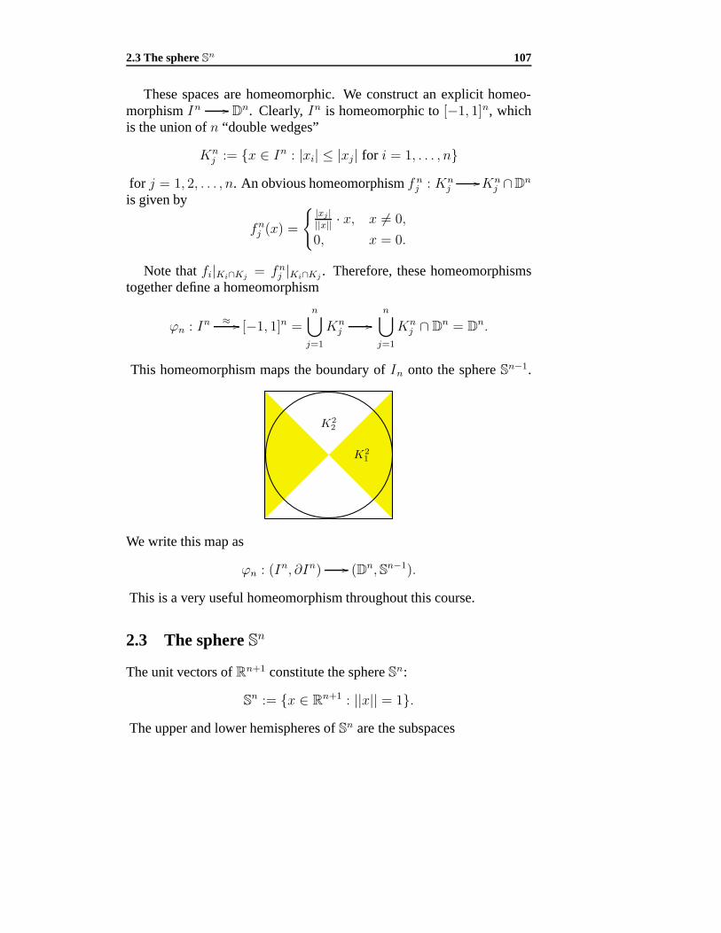
These spaces are homeomorphic. We construct an explicit homeo-morphism In Dn. Clearly, In is homeomorphic to [−1, 1]n, whichis the union of n “double wedges”
Knj := x ∈ In : |xi| ≤ |xj | for i = 1, . . . , n
for j = 1, 2, . . . , n. An obvious homeomorphism f nj : Kn
jKn
j ∩Dn
is given by
fnj (x) =
|xj |||x|| · x, x = 0,
0, x = 0.
Note that fi|Ki∩Kj= fn
j |Ki∩Kj. Therefore, these homeomorphisms
together define a homeomorphism
ϕn : In≈ [−1, 1]n =
n⋃j=1
Knj
n⋃
j=1
Knj ∩ D
n = Dn.
This homeomorphism maps the boundary of In onto the sphere Sn−1.
K21
K22
We write this map as
ϕn : (In, ∂In) (Dn, Sn−1).
This is a very useful homeomorphism throughout this course.
2.3 The sphere Sn
The unit vectors of Rn+1 constitute the sphere Sn:
Sn := x ∈ R
n+1 : ||x|| = 1.The upper and lower hemispheres of Sn are the subspaces
108 Homeomorphism
En+ := (x1, . . . , xn+1) ∈ S
n : xn+1 ≥ 0,E
n− := (x1, . . . , xn+1) ∈ S
n : xn+1 ≤ 0.Clearly,
En+ ∪ E
n− = S
n, En+ ∩ E
n− = S
n−1.
Each of these is homeomorphic to Dn. In each case, the projectiononto “the equatorial subspace” is a homeomorphism.
p± : (En±, S
n−1) (Dn, Sn−1).
The inverse homeomorphisms fε : Dn En±, ε = ±1, are given by
fε(x) = (x, ε√
1− ||x||2).
2.3.1 Stereographic projection
Stereographic projection from the “north pole” en+1 ∈ Sn onto the“equatorial” hyperplane gives a homeomorphism. Every point on Sn \en+1 is uniquely of the form cos θ · en+1 + sin θ · v for some unit vec-tor v ∈ e⊥n+1. Stereographic projection from en+1 sends this vector tocot θ
2· v.
Chapter 3
Quotient topology and one-pointcompactification
3.1 Quotient space
Let X be a topological space with an equivalence relation R. The quo-tient topology on X/R is characterized by the following: a functionX/R Y is continuous if and only if the composite X X/R Yis continuous. 1
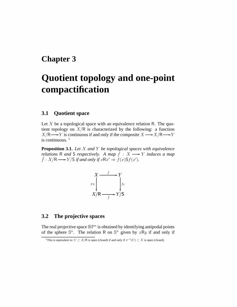
Proposition 3.1. Let X and Y be topological spaces with equivalencerelations R and S respectively. A map f : X Y induces a mapf : X/R Y/S if and only if xRx′ ⇒ f(x)Sf(x′).
X/R Y/Sf
X
X/R
pX
X Yf Y
Y/S
fY
3.2 The projective spaces
The real projective space RPn is obtained by identifying antipodal pointsof the sphere S
n. The relation R on Sn given by xRy if and only if
1This is equivalent to: U ⊂ X/R is open (closed) if and only if π−1(U) ⊂ X is open (closed).
110 Quotient topology and one-point compactification
x = ±y is an equivalence relation. Each equivalence class consists of apair of antipodal points x, −x ⊂ S
n.The real projective space RPn can also be viewed as the space of
(punctured) lines in Rn+1. This means that on Rn+1 \ 0 we definea relation R′ by xR′y if and only if x = ky for some nonzero k ∈ R.This is an equivalence relation. The inclusion map Sn Rn+1 respectsthe relation R: clearly, xRy in Sn implies xR′y in Rn+1. This induces abijection Sn/R Rn+1/R′, which is a homeomorphism.
3.2.1 Complex projective spaces
On the complex vector space Cn+1 the equivalence relation
z R z′ if and only if z = kz′ for some nonzero k ∈ C
yields the complex projective space CPn.The complex projective space CP1 is homeomorphic to S2.
3.3 Collapsing a closed subspace
Let A ⊂ X be a closed subspace. By identifying points in A we obtaina space X/A with the quotient topology. 2
Proposition 3.2. En+/S
n−1 is homeomorphic to Sn.
Proof. Every point in En+ can be written as cos θen+1 + sin θv for a
unit vector v ∈ Sn−1, and unique θ ∈ [0, π2]. The map which sends
this to cos 2θen+1 + sin 2θv maps the equator in −en+1, and induces acontinuous bijection En
+/Sn−1 Sn, which is necessarily a homemor-
phism.
3.4 One-point compactification
Let X be a topological space, The one-point compactification of X is
X∞ := X ∪ ∞, ∞ /∈ X,
topologized by stipulating that U ∈ X∞ is open if(i) ∞ /∈ U and U is open in X , or(ii) ∞ ∈ U and X∞ \ U is closed and compact in X .
2This means that we define a relation on X by xRy if and only if either x, y ∈ A or x, y /∈ A. This isan equivalence relation. The equivalence classes are the set A, and points in X \A.
3.4 One-point compactification 111
Then X∞ is compact, and X is dense in X∞.
Proposition 3.3. (Rn)∞ ≡ Sn.
Proof. Consider Rn imbedded in Rn+1 and take as ∞ the “north pole”of Sn, namely, N = (0, . . . , 0, 1). The stereographic projectionf : (Rn)∞ Sn given by
f(x) =
1
||x||2+1(2x, ||x||2 − 1) , x = N,
N, x = N,
is a continuous bijection from a compact space to a Hausdorff space.Hence it is a homeomorphism. It is enough to check the continuity atthe “infinite point”. If U is an open neighbourhood of N ⊂ Sn, itscomplement is a closed subset of Sn not containing N , and is compact.Under f , this corresponds to a compact subset of R
n. This shows that fis continuous at N .
Proposition 3.4. (1) X∞ is Hausdorff if X is locally compact and Hau-dorff.
(2) If X is compact Hausdorff and x ∈ X , then (X \ x)∞ ≡ X .
Proposition 3.5. If X is Haudorff and regular 3, U ⊂ X open, and Ucompact, then
X/(X \ U) ≡ U∞.
Proof. We construct a homeomorphism f : U∞ X/(X\U) by setting
f |U = U⊂ X
p X/(X \ U)
and f(∞) = [X \U ]. Clearly, f is a bijection. Since it maps a compactspace to a Hausdorff space, it is a homeomorphism if it is continuous.To prove this, we need only check the neighborhoods of [X \ U ]. If Vis an open neighborhood of [X \ U ], then W = p−1(V ) is an open setin X , and U \W is compact, being a closed set in the compact space U .Now,
f−1(V ) \ ∞ = W ∩ U = U \ (U \W )
is open in U . This shows that f−1(V ) is open in U∞, and f is continu-ous.
3A space is regular if each neighborhood of a point contains a closed neighborhood of the point. Acompact Hausdorff space is regular.
112 Quotient topology and one-point compactification
For example, if U is a bounded open subset of Rn, then
U∞ ≡ Rn/(Rn \ U).
Proposition 3.6.D
n/Sn−1 ≡ Sn.
Proof.
Dn/Sn−1 ≡In/∂In = In/(In \ intIn) ≡ (intIn)∞ ≡ (Rn)∞ ≡ S
n.
Chapter 4
Homotopy
Two maps f, g : X Y are homotopic if there exists a continuous mapH : X × I Y (called a homotopy) such that
H(x, 0) = f(x), H(x, 1) = g(x)
for x ∈ X .
Proposition 4.1. Homotopy is an equivalence relation on Y X .
[X, Y ] denotes the set of homotopy classes of maps from X to Y .
Examples
(1) If Y is a one-point space, there is only one mapping f : X Y ,and [X, Y ] is a singleton.
(2) If X is a one-point space, Y X is homemorphic to Y . Two mapsf, g : X Y are homotopic if and only if f(x) and g(x) are in the samepath component of Y . [X, Y ] is in one-to-one correspondence with thepath components of Y .
(3) Every map f : R Y is homotopic to a constant map. Here isa null-homotopy H : R × I Y :
H(x, t) = f(tx), x ∈ R, t ∈ I.
The same reasoning shows that every map Rn Y is null-homotopic(or homotopically trivial).
202 Homotopy
4.1 Homotopy equivalence
A map f : X Y is a homotopy equivalence if there exists a mapg : Y X such that
g f ∼ ιX and f g ∼ ιY .
In this case, g is said to be a homotopy inverse of f , and the spaces Xand Y are said to be homotopy equivalent.
A space is contractible if it is homotopy equivalent to a one-pointspace. Show that X is contractible if and only if every map f : X Yis homotopic to a constant map. Every euclidean space Rn is con-tractible.
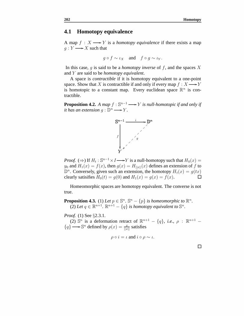
Proposition 4.2. A map f : Sn−1 Y is null-homotopic if and only ifit has an extension g : Dn Y .
Sn−1 Dni Sn−1
Y
f
Dn
Y
g
Proof. (⇒) If Ht : Sn−1×I Y is a null-homotopy such that H0(x) =y0 and H1(x) = f(x), then g(x) = H||x||(x) defines an extension of f toD
n. Conversely, given such an extension, the homotopy Ht(x) = g(tx)clearly satisifies H0(t) = g(0) and H1(x) = g(x) = f(x).
Homeomorphic spaces are homotopy equivalent. The converse is nottrue.
Proposition 4.3. (1) Let p ∈ Sn. S
n − p is homeomorphic to Rn.
(2) Let q ∈ Rn+1. Rn+1 − q is homotopy equivalent to Sn.
Proof. (1) See §2.3.1.(2) S
n is a deformation retract of Rn+1 − q, i.e., ρ : R
n+1 −q Sn defined by ρ(x) = x
||x|| satisfies
ρ i = ι and i ρ ∼ ι.
4.2 Nullhomotopy of Sm −→ Sn for m < n 203
4.2 Nullhomotopy of Sm −→ Sn for m < n
Theorem 4.4. If m < n, every map f : Sm −→ S
n is nullhomotopic.
Proof. Regard Sm as the boundary ∂K of an (m+1)-simplex. Subdivide∂K by iterated barycentric subdivision until each closed (n+1)-simplexis mapped into an open hemisphere of Sn. This is possible by the Lebe-gue covering theorem. Let ∂K be this subdivision. We construct a mapg : ∂K ′ Sn agreeing with f on the vertices, such that g is a homeo-morphism on each face of ∂K ′ and g ∼ f .
First, define h : ∂K ′ Rn+1 by f on vertices and extend linearlyover each simplex, i.e., for x =
∑li=1 λiei, put h(x) =
∑li=1 λif(ei).
Then define g(x) = h(x)||h(x)|| . Note that h(x) is never zero since the simplex
[f(e1), . . . , f(el)] is contained in an open hemisphere and its convexhull avoids the origin.
It is easy to construct a homotopy f ∼ g. In fact,
Ht(x) =(1− t)f(x) + tg(x)
||(1− t)f(x) + tg(x)||will do. We need only make sure that it is well defined. Since f(x) andg(x) lie in the same open hemisphere, the segment joining them avoidsthe origin.
Since g is a homeomorphism on each simplex of ∂K ′, its image isa finite union of m-cells and cannot be Sn if m < n. Let z ∈ Sn be apoint on in its image. Then g factors through a contractible space and isnullhomotopic. This shows that f is nullhomotopic.
THEOREM. The spheres Sm−1 and Sn−1 are homotopy equivalent ifand only if m = n.

204 Homotopy
Chapter 5
Homotopy functors and theirapplications
5.1 Categories and functors
Here are some examples of categories. Each consists of objects andmorphisms between them.
Category Objects MorphismsSet sets functionsTop topological spaces continuous functionsTop0 topological spaces with basepoints basepoint preserving mapsGrp groups homomorphismsAb abelian groups homomorphismsRing rings homomorphisms
vector spaces over R linear mapsVect(R) real vector bundles bundle maps
5.1.1 Covariant and contravariant functors
Let C and D be categories. A covariant functor F : C D is definedby(i) F(X) ∈ D for each object X ∈ C, and(ii) f∗ : F(X) F(Y ) in D for each f : X Y in C.
These are subject to(iii) (g f)∗ = g∗ f∗,(iv) (ιX)∗ = ιF(X).
There are also contravariant functors defined analogously, with (ii)
206 Homotopy functors and their applications
and (iii) replaced by(ii’) f ∗ : F(Y ) F(X) in D for each f : X Y in C;(iii) (g f)∗ = f ∗ g∗.
A functor F : Top0D is a homotopy functor if f ∼ g ⇒ f∗ = g∗.
Here are some examples of homotopy functors between such cate-gories.
Functor between categoriesFundamental group π1 : Top0
GrpHomotopy πn : Top0
AbHomology Hn : Top Abcohomology H∗ : Top Ring contravariant
5.2 An example: Brouwer’s fixed point theorem
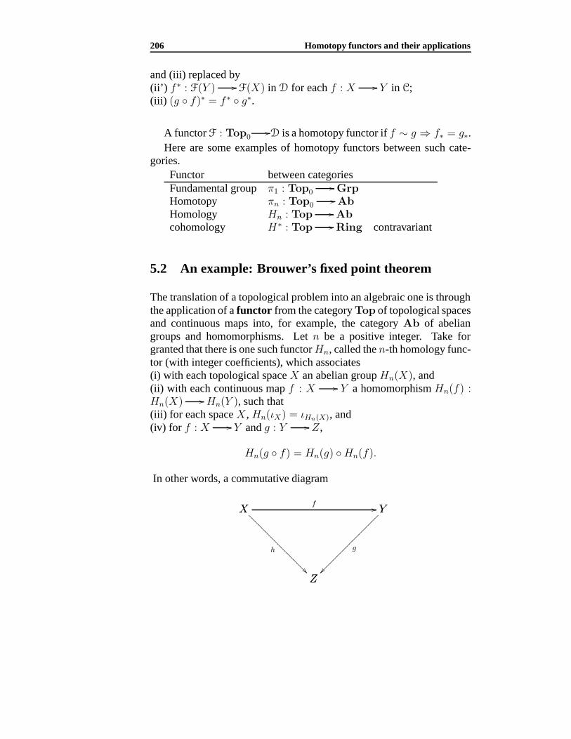
The translation of a topological problem into an algebraic one is throughthe application of a functor from the category Top of topological spacesand continuous maps into, for example, the category Ab of abeliangroups and homomorphisms. Let n be a positive integer. Take forgranted that there is one such functor Hn, called the n-th homology func-tor (with integer coefficients), which associates(i) with each topological space X an abelian group Hn(X), and(ii) with each continuous map f : X Y a homomorphism Hn(f) :Hn(X) Hn(Y ), such that(iii) for each space X , Hn(ιX) = ιHn(X), and(iv) for f : X Y and g : Y Z,
Hn(g f) = Hn(g) Hn(f).
In other words, a commutative diagram
X
Z
h
X Y
f Y
Z
g

5.2 An example: Brouwer’s fixed point theorem 207
in topology induces one in algebra:
Hn(X)
Hn(Z)
Hn(h)
Hn(X) Hn(Y )
Hn(f) Hn(Y )
Hn(Z)
Hn(g)
It is known that
Hn(Sm) =
Z, m = 0, n;
0, otherwise.
Also,Hn(D
m) = 0.
Theorem 5.1 (Brouwer’s fixed point theorem). Every map f : Dn+1 Dn+1
must have a fixed point.
Proof. Suppose, for a contradiction, that f : Dn+1 Dn+1 does not
have a fixed point. We can define a map g : Dn+1 Sn by letting g(x)be the intersection of the boundary sphere with the half line joining f(x)to the distinct point x.
x
f(x)
g(x)
Clearly, g(x) = x for x ∈ Sn. This means we have a commutativediagram
Sn
Sn
ι
Sn Dn+1g Dn+1
Sn
i
208 Homotopy functors and their applications
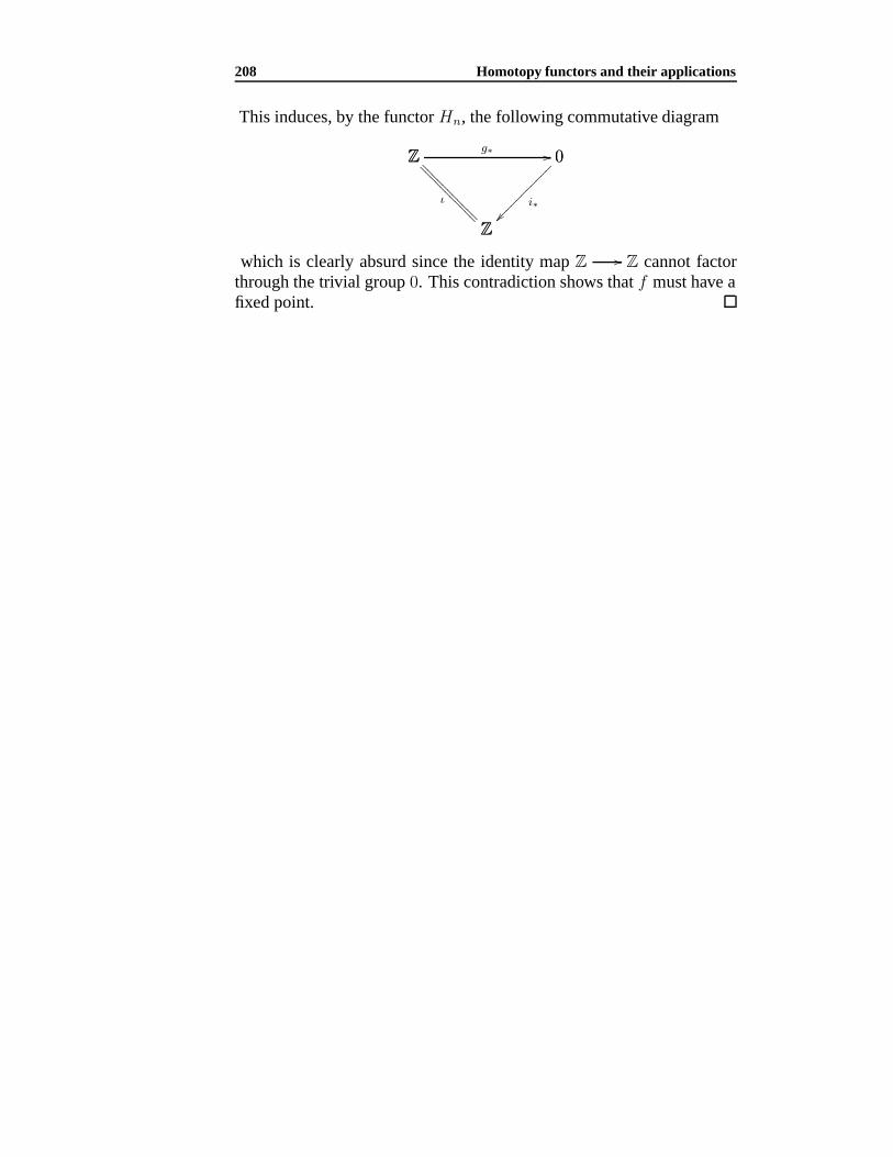
This induces, by the functor Hn, the following commutative diagram
Z
Z
ι
Z 0
g∗ 0
Z
i∗
which is clearly absurd since the identity map Z Z cannot factorthrough the trivial group 0. This contradiction shows that f must have afixed point.
Chapter 6
Euclidean spaces and theirlinear maps
We shall consider the euclidean space Rn equipped with an inner product
〈x, y〉 := xyt
for x, y ∈ Rn. Two vectors x, y ∈ R
n are orthogonal if 〈x, y〉 = 0.A basis of Rn consisting of mutually orthogonal unit vectors is calledan orthonormal basis. A most convenient orthonormal basis of Rn is thecanonical basis
e1, e2, . . . , en
in which, for k ≤ n, ek is the vector in Rn with a single nonzero entry 1
in its k-th position. Thus,
e1 =(1, 0, . . . , 0),
e2 =(0, 1, . . . , 0),
...
en =(0, 0, . . . , 0).
For k ≤ m ≤ n, we shall identify ek in Rm as ek in Rn. In fact, thereis a filtration of euclidean spaces
R1 ⊂ R
2 ⊂ · · · ⊂ Rn ⊂ · · ·
for which we can speak of the (co-)limit
R∞ :=
⋃n≥1
Rn
210 Euclidean spaces and their linear maps
consisting of vectors each of finitely many nonzero components. Thespace R
∞ is given the colimit topology. 1
6.1 Linear maps on euclidean spaces
6.1.1 The matrix of a linear map
Let f : Rm Rn be a linear map, with
f(ei) =
n∑j=1
ai,jej , i = 1, 2, . . . , m.
It is conveniently represented by the m× n matrix
A =
a1,1 a1,2 . . . a1,n
a2,1 a2,2 . . . a2,n
· · ·am,1 am,2 . . . an,n
If x =
∑mi=1 xiei is abbreviated to the 1×m matrix x =
(x1 x2 . . . xm
),
then f(x) = xA.
6.1.2 The adjoint of a linear map
The adjoint of f is the linear map f# : Rn Rm defined by
〈f(x), y〉 = 〈x, f#(y)〉, x ∈ Rm, y ∈ R
n.
The adjoint f# is represented by the transpose matrix of A.A map f : Rn Rn is self-adjoint if
〈f(x), y〉 = 〈x, f(y)〉, x, y ∈ Rn.
A self-adjoint map is represented by a symmetric matrix, i.e., ai,j = aj,ifor 1 ≤ i, j ≤ n.
1This means that a map f : R∞ Y is continuous if and only if each f ιn : R
n R∞ Yis continuous.

6.2 The spectral theorem on self-adjoint linear maps 211
6.1.3 Determinant
The determinant of a linear map f : Rn Rn is the unique real numberdet f satisfying
f(v1) ∧ · · · ∧ f(vn) = det f · (v1 ∧ · · · ∧ vn).
6.2 The spectral theorem on self-adjoint linear maps
Theorem 6.1. Let A be a real n × n symmetric matrix. There is anorthonormal basis of eigenvectors v1, . . . , vn with corresponding realeigenvalues.
Proof. Consider the real valued function F : Sn−1 R defined by
F (x) = 〈xA, x〉.Since the domain is compact, F assumes a maximum value λ, say, atv ∈ Sn−1. We show that vA = λv (so that v is an eigenvector with realeigenvalue λ). From f(v) = λ, we have 〈vA− λv, v〉 = 0. This meansvA = λv + w for some w ⊥ v. Since A is symmetric,
〈wA, v〉 = 〈w, vA〉 = 〈w, λv + w〉 = 〈w, w〉.
If w = 0, then for arbitrary t ∈ R, F (v + tw) ≤ λ implies
t2〈wA, w〉 ≤ (λt2 − 2t)〈w, w〉for arbitrary t ∈ R. Consequently, 〈w, w〉 = 0 and w = 0, contradictingthe assumption w = 0.
This shows that w = 0, vA = λv, and v is a unit eigenvector of A.The same reasoning applied to the orthogonal complement of v shows
that there is an eigenvector v2 of A corresponding to an eigenvalue λ2
which is the maximum of F restricted to Sn−1 ∩ v⊥. By induction, weobtain an orthonormal basis v1, v2, . . . , vn of unit eigenvectors of Awith corresponding eigenvalues λ1 ≥ λ2 ≥ · · · ≥ λn such that λ1 isthe maximum of F , and for k = 2, . . . , n, λk is the maximum of F onSn−1 ∩ span(v1, . . . , vk−1)
⊥.
212 Euclidean spaces and their linear maps
6.3 Isometries of Rn
Let τ : Rn Rn be an isometry, i.e., ||τ(x)|| = ||x|| for every x ∈ Rn.The only possible real eigenvalues of τ are ε = ±1. For each ε, we
have an invariant subspace Vε := x ∈ Rn : τ(x) = εx.V := V+
⊕V− is also an invariant subspace of τ . If V = Rn, then
τ has a complex (non-real) eigenvalue, corresponding to which is aninvariant 2-plane with an orthonormal basis u, v such that
τ(u) = cos θ · u+ sin θ · v,τ(v) =− sin θ · u+ cos θ · v,
for some θ ∈ R.
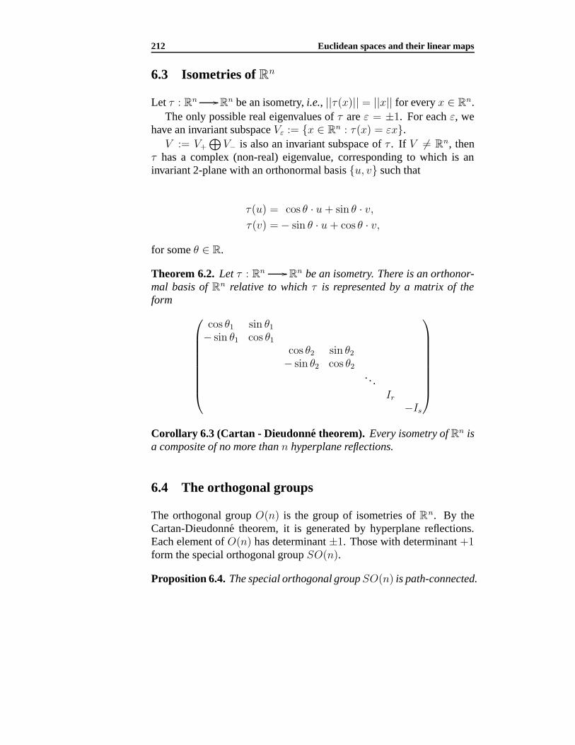
Theorem 6.2. Let τ : Rn Rn be an isometry. There is an orthonor-
mal basis of Rn relative to which τ is represented by a matrix of theform
cos θ1 sin θ1
− sin θ1 cos θ1
cos θ2 sin θ2
− sin θ2 cos θ2
. . .Ir
−Is
Corollary 6.3 (Cartan - Dieudonne theorem). Every isometry of R
n isa composite of no more than n hyperplane reflections.
6.4 The orthogonal groups
The orthogonal group O(n) is the group of isometries of Rn. By theCartan-Dieudonne theorem, it is generated by hyperplane reflections.Each element of O(n) has determinant ±1. Those with determinant +1form the special orthogonal group SO(n).
Proposition 6.4. The special orthogonal groupSO(n) is path-connected.
6.4 The orthogonal groups 213
6.4.1 The hyperplane reflection map
Let x ∈ Rn be a unit vector. We consider the reflection in the hyperplanewhich is the orthogonal complement of x in Rn. This is the isometryρx : Rn Rn defined by
ρx(y) = y − 2〈x, y〉x.This is an orientation reversing isometry and so has determinant −1.
The hyperplane reflection map ρ : Sn−1 O(n) given by ρ(x) = ρx isa very important map in this course.
Chapter 7
The quaternions and theoctonions
7.1 The quaternions
The quaternions are generalizations of the complex numbers. Let C bethe field of complex numbers, with the notions of conjugation and norm.The quaternion algebra is H = C ⊕ C with conjugation and multiplica-tion defined by
(u, v) := (u, −v),(u1, v1)(u2, v2) := (u1u2 − v2v1, v1u2 + v2u1).
(7.1)
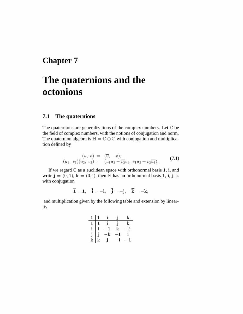
If we regard C as a euclidean space with orthonormal basis 1, i, andwrite j = (0, 1), k = (0, i), then H has an orthonormal basis 1, i, j, kwith conjugation
1 = 1, i = −i, j = −j, k = −k,
and multiplication given by the following table and extension by linear-ity
1 1 i j k1 1 i j ki i −1 k −jj j −k −1 ik k j −i −1
302 The quaternions and the octonions
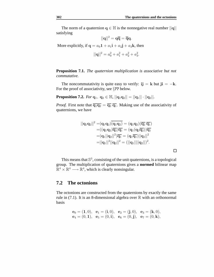
The norm of a quaternion q ∈ H is the nonnegative real number ||q||satisfying
||q||2 = qq = qq.
More explicitly, if q = a01 + a1i + a2j + a3k, then
||q||2 = a20 + a2
1 + a22 + a2
3.
Proposition 7.1. The quaternion multiplication is associative but notcommutative.
The noncommutativity is quite easy to verify: ij = k but ji = −k.For the proof of associativity, see §?? below.
Proposition 7.2. For q1, q2 ∈ H, ||q1q2|| = ||q1|| · ||q2||.Proof. First note that q1q2 = q2 q1. Making use of the associativity ofquaternions, we have
||q1q2||2 =(q1q2)(q1q2) = (q1q2)(q2 q1)
=((q1q2)q2)q1 = (q1(q2q2))q1
=(q1||q2||2)q1 = (q1q1)||q2||2=||q1||2||q2||2 = (||q1||||q2||)2.
This means that S3, consisting of the unit quaternions, is a topologicalgroup. The multiplication of quaternions gives a normed bilinear mapR4 × R4 −→ R4, which is clearly nonsingular.
7.2 The octonions
The octonions are constructed from the quaternions by exactly the samerule in (7.1). It is an 8-dimensional algebra over R with an orthonormalbasis
e0 = (1, 0), e1 = (i, 0), e2 = (j, 0), e3 = (k, 0),e4 = (0, 1), e5 = (0, i), e6 = (0, j), e7 = (0,k),
7.3 The Cayley-Dickson algebras 303
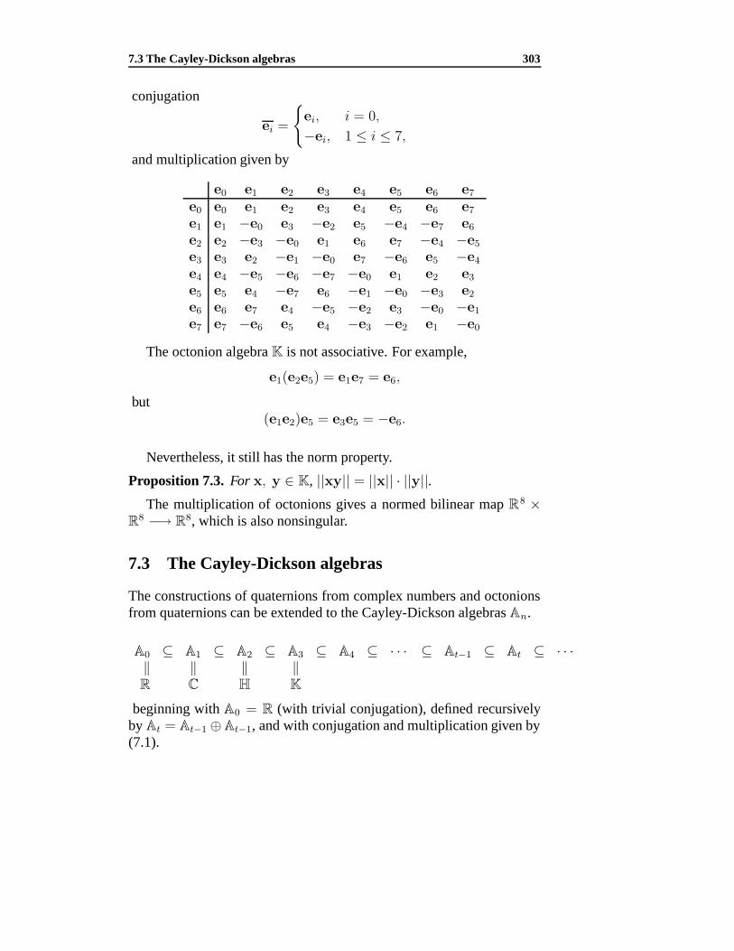
conjugation
ei =
ei, i = 0,
−ei, 1 ≤ i ≤ 7,
and multiplication given by
e0 e1 e2 e3 e4 e5 e6 e7
e0 e0 e1 e2 e3 e4 e5 e6 e7
e1 e1 −e0 e3 −e2 e5 −e4 −e7 e6
e2 e2 −e3 −e0 e1 e6 e7 −e4 −e5
e3 e3 e2 −e1 −e0 e7 −e6 e5 −e4
e4 e4 −e5 −e6 −e7 −e0 e1 e2 e3
e5 e5 e4 −e7 e6 −e1 −e0 −e3 e2
e6 e6 e7 e4 −e5 −e2 e3 −e0 −e1
e7 e7 −e6 e5 e4 −e3 −e2 e1 −e0
The octonion algebra K is not associative. For example,
e1(e2e5) = e1e7 = e6,
but(e1e2)e5 = e3e5 = −e6.
Nevertheless, it still has the norm property.
Proposition 7.3. For x, y ∈ K, ||xy|| = ||x|| · ||y||.The multiplication of octonions gives a normed bilinear map R8 ×
R8 −→ R8, which is also nonsingular.
7.3 The Cayley-Dickson algebras
The constructions of quaternions from complex numbers and octonionsfrom quaternions can be extended to the Cayley-Dickson algebras An.
A0 ⊆ A1 ⊆ A2 ⊆ A3 ⊆ A4 ⊆ · · · ⊆ At−1 ⊆ At ⊆ · · ·‖ ‖ ‖ ‖R C H K
beginning with A0 = R (with trivial conjugation), defined recursivelyby At = At−1 ⊕ At−1, and with conjugation and multiplication given by(7.1).

304 The quaternions and the octonions
7.3.1 Commutators and associators in Cayley-Dickson algebras
An element x in a Cayley-Dickson algebra At is pure if x+ x = 0. Thepure part of x is the element x := 1
2(x− x). Let x, y, z ∈ At.
(1) [x, y] := xy−yx is called the commutator of x and y. The algebraA is commutative if all commutators are zero.
(2) (x, y, z) := (xy)z − x(yz) is called the associator of x, y, z. Thealgebra A is associative if all associators are zero.
(3) At is said to be alternative if (x, x, y) = (y, x, x) = 0 for allx, y ∈ At.
Proposition 7.4. The commutators and associators of At are related tothose of At−1 as follows.
[(x1, y1), (x2, y2)] = ([x1, x2]− [y1, y2], 2(y2x1 − y1x2)).
((x1, y1), (x2, y2), (x3, y3)) = (Φ,Ψ),
where
Φ = (x1, x2, x3)− (x3, y2, y1) + (x2, y3, y1)− (y3, y2, x1) + (y3, y1, x2)+[x1, y3y2]− [x2, y3y1] + [x3, y2y1];
Ψ = (y1, y2, y3) + (y1, x2, x3)− (y3, x2, x1) + (y2, x3, x1)− (y2, x1, x3)+y1[x2, x3]− y2[x1, x3] + y3[x1, x2]− y3[y2, y1]− [y3, y1y2].
Proposition 7.5. The Cayley-Dickson algebra At is(i) alternative if and only if At−1 is associative;(ii) associative if and only if At−1 is associative and commutative.
Here is the multiplication table of the Cayley-Dickson algebra A4.
+e0 +e1 +e2 +e3 +e4 +e5 +e6 +e7 +e8 +e9 +e10 +e11 +e12 +e13 +e14 +e15+e1 −e0 +e3 −e2 +e5 −e4 −e7 +e6 +e9 −e8 −e11 +e10 −e13 +e12 +e15 −e14+e2 −e3 −e0 +e1 +e6 +e7 −e4 −e5 +e10 +e11 −e8 −e9 −e14 −e15 +e12 +e13+e3 +e2 −e1 −e0 +e7 −e6 +e5 −e4 +e11 −e10 +e9 −e8 −e15 +e14 −e13 +e12+e4 −e5 −e6 −e7 −e0 +e1 +e2 +e3 +e12 +e13 +e14 +e15 −e8 −e9 −e10 −e11+e5 +e4 −e7 +e6 −e1 −e0 −e3 +e2 +e13 −e12 +e15 −e14 +e9 −e8 +e11 −e10+e6 +e7 +e4 −e5 −e2 +e3 −e0 −e1 +e14 −e15 −e12 +e13 +e10 −e11 −e8 +e9+e7 −e6 +e5 +e4 −e3 −e2 +e1 −e0 +e15 +e14 −e13 −e12 +e11 +e10 −e9 −e8+e8 −e9 −e10 −e11 −e12 −e13 −e14 −e15 −e0 +e1 +e2 +e3 +e4 +e5 +e6 +e7+e9 +e8 −e11 +e10 −e13 +e12 +e15 −e14 −e1 −e0 −e3 +e2 −e5 +e4 +e7 −e6
+e10 +e11 +e8 −e9 −e14 −e15 +e12 +e13 −e2 +e3 −e0 −e1 −e6 −e7 +e4 +e5+e11 −e10 +e9 +e8 −e15 +e14 −e13 +e12 −e3 −e2 +e1 −e0 −e7 +e6 −e5 +e4+e12 +e13 +e14 +e15 +e8 −e9 −e10 −e11 −e4 +e5 +e6 +e7 −e0 −e1 −e2 −e3+e13 −e12 +e15 −e14 +e9 +e8 +e11 −e10 −e5 −e4 +e7 −e6 +e1 −e0 +e3 −e2+e14 −e15 −e12 +e13 +e10 −e11 +e8 +e9 −e6 −e7 −e4 +e5 +e2 −e3 −e0 +e1+e15 +e14 −e13 −e12 +e11 +e10 −e9 +e8 −e7 +e6 −e5 −e4 +e3 +e2 −e1 −e0
7.4 Appendix: zero divisors in A4 305
7.4 Appendix: zero divisors in A4
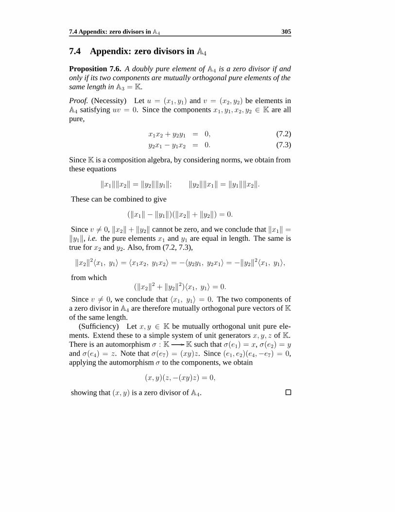
Proposition 7.6. A doubly pure element of A4 is a zero divisor if andonly if its two components are mutually orthogonal pure elements of thesame length in A3 = K.
Proof. (Necessity) Let u = (x1, y1) and v = (x2, y2) be elements inA4 satisfying uv = 0. Since the components x1, y1, x2, y2 ∈ K are allpure,
x1x2 + y2y1 = 0, (7.2)
y2x1 − y1x2 = 0. (7.3)
Since K is a composition algebra, by considering norms, we obtain fromthese equations
‖x1‖‖x2‖ = ‖y2‖‖y1‖; ‖y2‖‖x1‖ = ‖y1‖‖x2‖.These can be combined to give
(‖x1‖ − ‖y1‖)(‖x2‖+ ‖y2‖) = 0.
Since v = 0, ‖x2‖+ ‖y2‖ cannot be zero, and we conclude that ‖x1‖ =‖y1‖, i.e. the pure elements x1 and y1 are equal in length. The same istrue for x2 and y2. Also, from (7.2, 7.3),
‖x2‖2〈x1, y1〉 = 〈x1x2, y1x2〉 = −〈y2y1, y2x1〉 = −‖y2‖2〈x1, y1〉,from which
(‖x2‖2 + ‖y2‖2)〈x1, y1〉 = 0.
Since v = 0, we conclude that 〈x1, y1〉 = 0. The two components ofa zero divisor in A4 are therefore mutually orthogonal pure vectors of K
of the same length.(Sufficiency) Let x, y ∈ K be mutually orthogonal unit pure ele-
ments. Extend these to a simple system of unit generators x, y, z of K.There is an automorphism σ : K K such that σ(e1) = x, σ(e2) = yand σ(e4) = z. Note that σ(e7) = (xy)z. Since (e1, e2)(e4,−e7) = 0,applying the automorphism σ to the components, we obtain
(x, y)(z,−(xy)z) = 0,
showing that (x, y) is a zero divisor of A4.

306 The quaternions and the octonions
Chapter 8
Quaternions and isometries inR
4
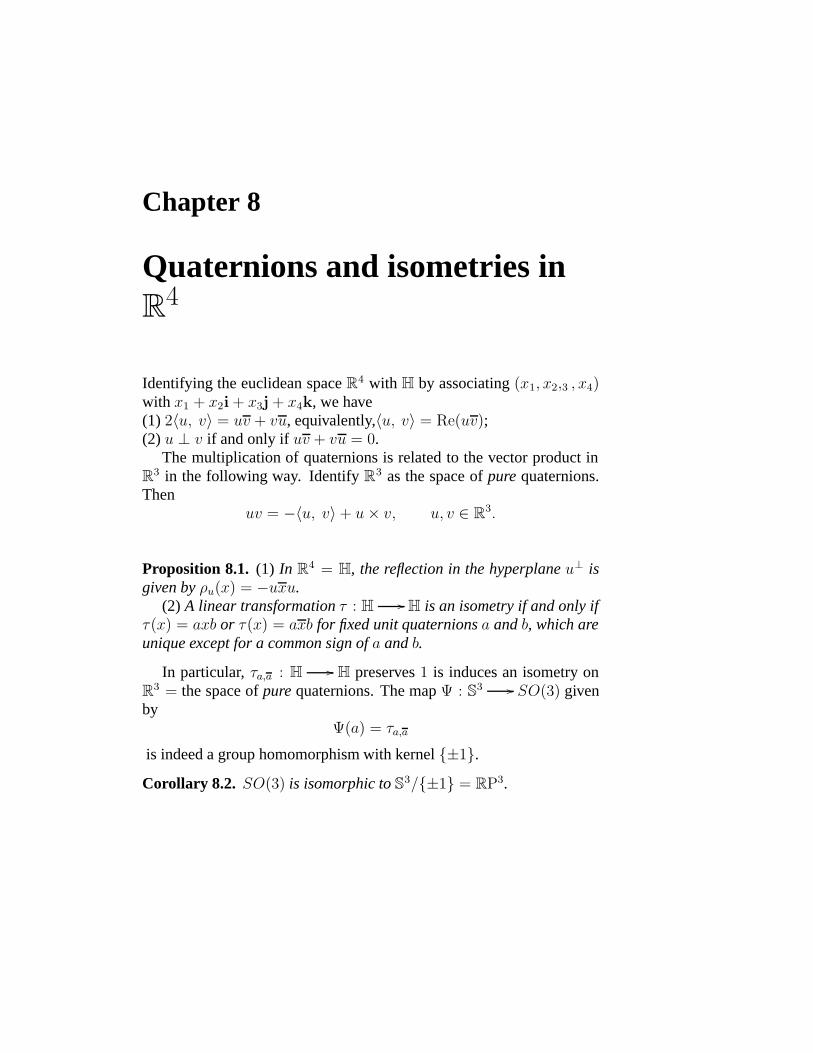
Identifying the euclidean space R4 with H by associating (x1, x2,3 , x4)with x1 + x2i + x3j + x4k, we have(1) 2〈u, v〉 = uv + vu, equivalently,〈u, v〉 = Re(uv);(2) u ⊥ v if and only if uv + vu = 0.
The multiplication of quaternions is related to the vector product inR
3 in the following way. Identify R3 as the space of pure quaternions.
Thenuv = −〈u, v〉+ u× v, u, v ∈ R
3.
Proposition 8.1. (1) In R4 = H, the reflection in the hyperplane u⊥ isgiven by ρu(x) = −uxu.
(2) A linear transformation τ : H H is an isometry if and only ifτ(x) = axb or τ(x) = axb for fixed unit quaternions a and b, which areunique except for a common sign of a and b.
In particular, τa,a : H H preserves 1 is induces an isometry onR
3 = the space of pure quaternions. The map Ψ : S3 SO(3) given
byΨ(a) = τa,a
is indeed a group homomorphism with kernel ±1.
Corollary 8.2. SO(3) is isomorphic to S3/±1 = RP3.

308 Quaternions and isometries in R4
Chapter 9
Normed bilinear maps and theirHopf constructions
9.1 Hurwitz’s theorem
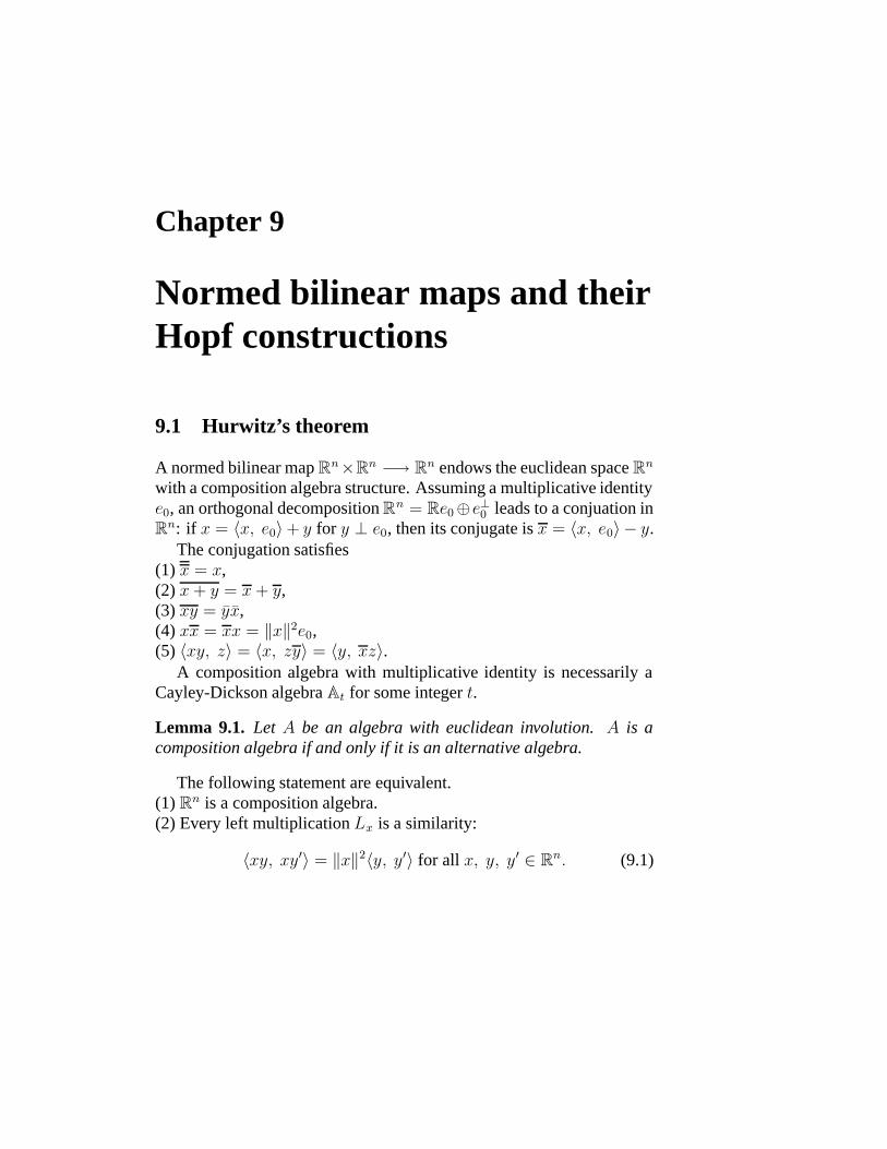
A normed bilinear map Rn×Rn −→ Rn endows the euclidean space Rn
with a composition algebra structure. Assuming a multiplicative identitye0, an orthogonal decomposition R
n = Re0⊕e⊥0 leads to a conjuation inRn: if x = 〈x, e0〉+ y for y ⊥ e0, then its conjugate is x = 〈x, e0〉 − y.
The conjugation satisfies(1) x = x,(2) x+ y = x+ y,(3) xy = yx,(4) xx = xx = ‖x‖2e0,(5) 〈xy, z〉 = 〈x, zy〉 = 〈y, xz〉.
A composition algebra with multiplicative identity is necessarily aCayley-Dickson algebra At for some integer t.
Lemma 9.1. Let A be an algebra with euclidean involution. A is acomposition algebra if and only if it is an alternative algebra.
The following statement are equivalent.(1) Rn is a composition algebra.(2) Every left multiplication Lx is a similarity:
〈xy, xy′〉 = ‖x‖2〈y, y′〉 for all x, y, y′ ∈ Rn. (9.1)

310 Normed bilinear maps and their Hopf constructions
(2’) Every right multiplication Ry is a similarity:
〈xy, x′y〉 = ‖y‖2〈x, x′〉 for all x, x′, y ∈ Rn. (9.2)
(3) For all x, y, x′, y′ ∈ Rn,
〈xy, x′y′〉+ 〈xy′, x′y〉 = 2〈x, x′〉〈y, y′〉. (9.3)
Theorem 9.2 (Hurwitz). The euclidean space Rn has a compositionalgebra structure if and only if n = 1, 2, 4, 8.
9.2 Normed bilinear maps and Hopf construction
A bilinear map f : Rr × Rs −→ Rn is said to be normed if
||f(x, y)|| = ||x|| · ||y||, x ∈ Rr, y ∈ R
s.
A normed bilinear map is nonsingular. Such a map gives a genuine mapbetween euclidean spheres.
Proposition 9.3. A normed bilinear map f : Rr ×Rs −→ Rn induces ahomogeneous quadratic map F : Sr+s−1 −→ Sn via the Hopf construc-tion
F (x, y) = (||x||2 − ||y||2, 2f(x, y)), x ∈ Rr, y ∈ R
s.
Proof. For x ∈ Rr, y ∈ Rs,
||F (x, y)||2 =(||x||2 − ||y||2)2 + ||2f(x, y)||2=(||x||2 − ||y||2)2 + 4||x||2||y||2=(||x||2 + ||y||2)2.
Therefore, (x, y) ∈ Sr+s−1 ⇒ F (x, y) ∈ Sn.
9.2.1 The classical Hopf maps
Applying the Hopf construction to normed bilinear maps Rn × Rn −→Rn for n = 1, 2, 4, 8, we obtain the following Hopf maps.
normed bilinear map Hopf mapR1 × R1 −→ R1 2 : S1 −→ S1
R2 × R2 −→ R2 η : S3 −→ S2
R4 × R4 −→ R4 ν : S7 −→ S4
R8 × R8 −→ R8 σ : S15 −→ S8
9.2 Normed bilinear maps and Hopf construction 311
The maps η, µ, σ are called the classical Hopf maps.
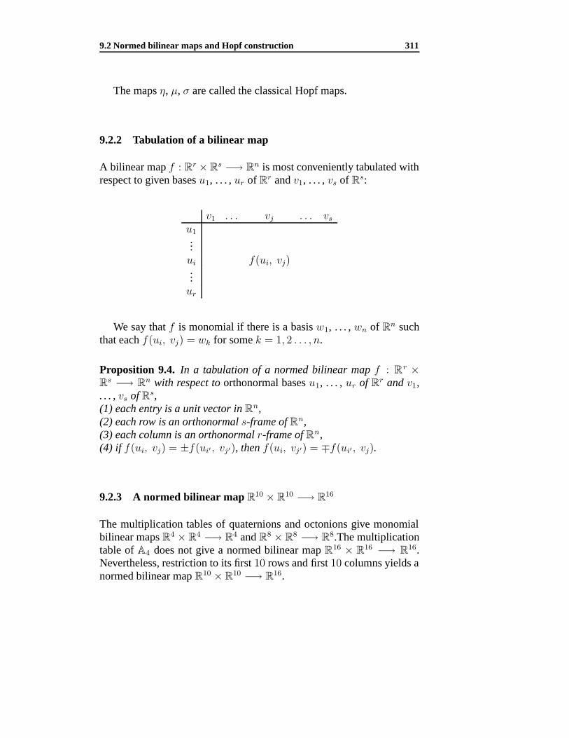
9.2.2 Tabulation of a bilinear map
A bilinear map f : Rr × Rs −→ Rn is most conveniently tabulated withrespect to given bases u1, . . . , ur of Rr and v1, . . . , vs of Rs:
v1 . . . vj . . . vsu1...ui f(ui, vj)...ur
We say that f is monomial if there is a basis w1, . . . , wn of Rn suchthat each f(ui, vj) = wk for some k = 1, 2 . . . , n.
Proposition 9.4. In a tabulation of a normed bilinear map f : Rr ×Rs −→ Rn with respect to orthonormal bases u1, . . . , ur of Rr and v1,. . . , vs of Rs,(1) each entry is a unit vector in Rn,(2) each row is an orthonormal s-frame of Rn,(3) each column is an orthonormal r-frame of Rn,(4) if f(ui, vj) = ±f(ui′, vj′), then f(ui, vj′) = ∓f(ui′, vj).
9.2.3 A normed bilinear map R10 × R10 −→ R16
The multiplication tables of quaternions and octonions give monomialbilinear maps R4 × R4 −→ R4 and R8 × R8 −→ R8.The multiplicationtable of A4 does not give a normed bilinear map R16 × R16 −→ R16.Nevertheless, restriction to its first 10 rows and first 10 columns yields anormed bilinear map R10 × R10 −→ R16.
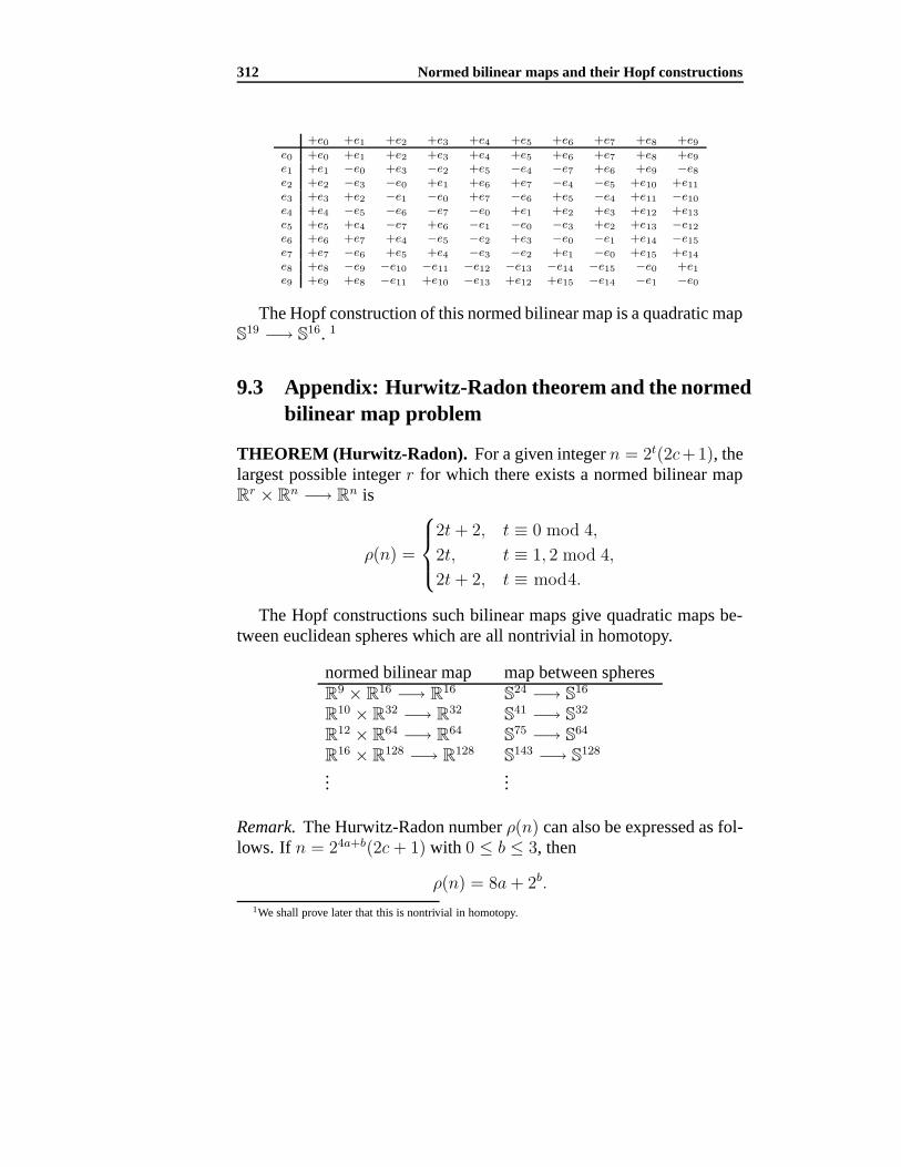
312 Normed bilinear maps and their Hopf constructions
+e0 +e1 +e2 +e3 +e4 +e5 +e6 +e7 +e8 +e9e0 +e0 +e1 +e2 +e3 +e4 +e5 +e6 +e7 +e8 +e9e1 +e1 −e0 +e3 −e2 +e5 −e4 −e7 +e6 +e9 −e8e2 +e2 −e3 −e0 +e1 +e6 +e7 −e4 −e5 +e10 +e11e3 +e3 +e2 −e1 −e0 +e7 −e6 +e5 −e4 +e11 −e10e4 +e4 −e5 −e6 −e7 −e0 +e1 +e2 +e3 +e12 +e13e5 +e5 +e4 −e7 +e6 −e1 −e0 −e3 +e2 +e13 −e12e6 +e6 +e7 +e4 −e5 −e2 +e3 −e0 −e1 +e14 −e15e7 +e7 −e6 +e5 +e4 −e3 −e2 +e1 −e0 +e15 +e14e8 +e8 −e9 −e10 −e11 −e12 −e13 −e14 −e15 −e0 +e1e9 +e9 +e8 −e11 +e10 −e13 +e12 +e15 −e14 −e1 −e0
The Hopf construction of this normed bilinear map is a quadratic mapS19 −→ S16. 1
9.3 Appendix: Hurwitz-Radon theorem and the normedbilinear map problem
THEOREM (Hurwitz-Radon). For a given integer n = 2t(2c+1), thelargest possible integer r for which there exists a normed bilinear mapRr × Rn −→ Rn is
ρ(n) =
2t+ 2, t ≡ 0 mod 4,
2t, t ≡ 1, 2 mod 4,
2t+ 2, t ≡ mod4.
The Hopf constructions such bilinear maps give quadratic maps be-tween euclidean spheres which are all nontrivial in homotopy.
normed bilinear map map between spheresR9 × R16 −→ R16 S24 −→ S16
R10 × R32 −→ R32 S41 −→ S32
R12 × R64 −→ R64 S75 −→ S64
R16 × R128 −→ R128 S143 −→ S128
......
Remark. The Hurwitz-Radon number ρ(n) can also be expressed as fol-lows. If n = 24a+b(2c+ 1) with 0 ≤ b ≤ 3, then
ρ(n) = 8a+ 2b.
1We shall prove later that this is nontrivial in homotopy.
9.3 Appendix: Hurwitz-Radon theorem and the normed bilinear map problem313
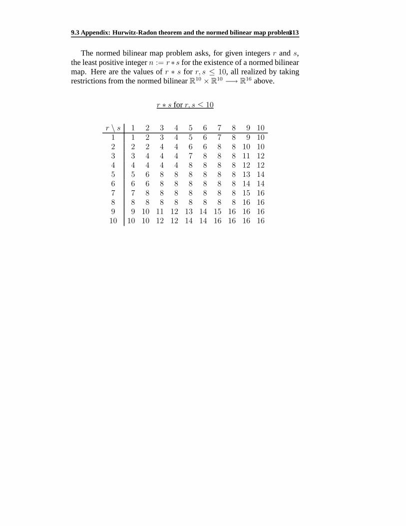
The normed bilinear map problem asks, for given integers r and s,the least positive integer n := r ∗s for the existence of a normed bilinearmap. Here are the values of r ∗ s for r, s ≤ 10, all realized by takingrestrictions from the normed bilinear R10 × R10 −→ R16 above.
r ∗ s for r, s ≤ 10
r \ s 1 2 3 4 5 6 7 8 9 101 1 2 3 4 5 6 7 8 9 102 2 2 4 4 6 6 8 8 10 103 3 4 4 4 7 8 8 8 11 124 4 4 4 4 8 8 8 8 12 125 5 6 8 8 8 8 8 8 13 146 6 6 8 8 8 8 8 8 14 147 7 8 8 8 8 8 8 8 15 168 8 8 8 8 8 8 8 8 16 169 9 10 11 12 13 14 15 16 16 1610 10 10 12 12 14 14 16 16 16 16
Chapter 10
Polynomial maps betweenspheres
We consider mappings between euclidean spheres whose componentfunctions of polynomials. A polynomial map F : Rm+1 → Rn+1 re-stricts to a map f : Sm → Sn if
F1(x)2 + F2(x)
2 + · · ·+ Fn+1(x)2 = 1
whenever ||x||2 = x21 + x2
2 + · · ·+ x2m+1 = 1. If the component func-
tions are homogeneous polynomials of degree d, this condition becomes||F (x)||2 = ||x||2d.
10.1 Wood’s theorem
Theorem 10.1 (Wood). If m ≥ 2t > n for some integer t, then everypolynomial map Sm −→ Sn must be constant.
We shall make use of two beautiful theorems discovered in the 1960’s.
THEOREM (Cassels). x21 + x2
2 + · · ·+ x2n cannot be written as a sum
of fewer than n squares of rational functions in x1, x2, . . . , xn.
Theorem 10.2 (Pfister). In a field of characteristic = 2, the product oftwo sums of 2t squares is again a sum of 2t squares.
10.1.1 Proof of Wood’s theorem: homogeneous case
It is enough to take m = 2t and n = 2t−1 and show that the assumptionof a homogeneous map F : Sm −→ Sn of degree d leads to a contradic-
402 Polynomial maps between spheres
tion. Such a map satisfies ||F (x)||2 = ||x||2d for every x ∈ Sm. Writex = (y, z) for y ∈ R
m, z ∈ R, and separate F into two parts, onecontaining even powers of z and the other odd powers of z:
F (x) = P (x) +Q(x)z,
where the components of P (x) and Q(x) are polynomials containingonly even powers of z. Since ||F (x)||2 = ||x||2d, we have
(||y||2 + z2)d =||P (x) +Q(x)z||2=||P (x)||2 + ||Q(x)||2z2 + 2z〈P (x), Q(x)〉.
Matching odd and even powers of z, we conclude
||P (x)||2 + ||Q(x)||2z2 =(||y||2 + z2)d, (10.1)
〈P (x), Q(x)〉 =0. (10.2)
Since P (x) and Q(x) contain only even powers of z, it makes senseto substitute z2 by −||y||2 in (10.1) and (10.2) so that P (x) and Q(x)become p(y) and q(y) for polynomials p and q satisfying
||p(y)||2 − ||q(y)||2||y||2 =0, (10.3)
〈p(y), q(y)〉 =0. (10.4)
From (10.3), we have
||y||2 = ||p(y)||2||q(y)||2 . (10.5)
Note that this expresses a sum of m = 2t squares as a quotient (henceproduct) of two sums of m = 2t squares. This is in conformity withPfister’s theorem. However, Wood observed a contradiction by addingz2 to both sides:
||y||2 + z2 =||p(y)||2||q(y)||2 + z2
=||p(y)||2 + ||q(y)||2z2
||q(y)||2
=||p(y) + q(y)z||2
||q(y)||2 .
This expresses y21 + y2
2 + · · ·+ y2m + z2 as a quotient (hence product) of
two sums of 2t squares, which by Pfister’s theorem, is a sum of m = 2t
squares, contradicting Cassels’ theorem.
10.2 Appendix: Pfister’s theorem 403
10.1.2 Proof of Wood’s theorem: general case
We reduce this to the homogeneous case. If all monomials in F haveeven degrees, with 2d the maximum of these degrees, then F can bemade homogeneous, without change in value, by multiplying each mono-mial of degree 2e by ||x||2(d−e). Such a map must be constant. Therefore,F is constant.
Suppose F contains some monomials of odd degree. The compositeF ′ = F α : Sm → Sm → Sn, where
α(x1, x2, . . . , xm+1) = (x21 − x2
2 − · · · − x2m+1, 2x1x2, · · · , 2x1xm+1)
has all monomials of even degrees. Such an F must be constant. Sinceα is surjective, F must be a constant map.
10.2 Appendix: Pfister’s theorem
An identity of the form
(x21 + x2
2 + · · ·+ x2n)(y
21 + y2
2 + · · ·+ y2n) = z2
1 + z22 + · · ·+ z2
n
in which z1, z2, . . . , zn are linear in y1, y2, . . . , yn is equivalent to ann× n matrix M satisfying
M tM = (x21 + · · ·+ x2
n)In.
Note that this entails MM t = (x21 + · · ·+ x2
n)In. It is well known thatsuch a matrix M exists for n = 1, 2, 4, 8, in which the entries are linearforms in x1, x2, . . . , xn. Assuming such matrices of order n, in whichthe entries are rational functions of x1, . . . , xn, we show that a matrix oforder 2n also exists satisfying
T tT = (x21 + · · ·+ x2
n + x2n+1 + · · ·+ x2
2n)I2n. (10.6)
Let M1 and M2 be n× n matrices satisfying
M t1M1 = M1M
t1 =(x2
1 + · · ·+ x2n)In,
M t2M2 = M2M
t2 =(x2
n+1 + · · ·+ x22n)In.
We try to find a matrix X such that T =
(M1 M2
M2 X
)satisfies (10.6).
404 Polynomial maps between spheres
The condition
T tT =
(M t
1 M t2
M t2 X t
)(M1 M2
M2 X
)=
(M t
1M1 +M t2M2 M t
1M2 +M t2X
M t2M1 +X tM2 M t
2M2 +X tX
).
We require the off-diagonal blocks to be zero. These both lead toM t
2X = −M t1M2. Explicitly,
X =
( −1
x2n+1 + · · ·+ x2
2n
)M2M
t1M2.
From this,
(M t2X)t(M t
2X) = (−M t2M1)(−M t
1M2)
⇒X t(M2Mt2)X = M t
2(M1Mt1)M2
⇒(M2Mt2)(X
tX) = (M t2M2)(M1M
t1)
⇒X tX = (x21 + · · ·+ x2
n)In,
and (10.6) follows.
Chapter 11
Nonsingular bilinear maps
11.1 Nonsingular bilinear maps on euclidean spaces
A bilinear map f : Rr × Rs −→ Rn is said to be nonsingular iff(x, y) = 0 ⇒ x = or y = 0. Normed bilinear maps are nonsingu-lar.
Examples
1. There is an obvious nonsingular bilinear map Rr × Rs −→ Rrs in-duced by matrix multiplication:
f(x, y) = xyt.
2. This example can be improved by lowering the dimension of therange, by making use of polynomial multiplications. Identify R
∞ withthe polynomial ring R[T ]. Polynomial multiplication clearly induces anonsingular bilinear map R∞ × R∞ −→ R∞. This retricts to a non-singular bilinear map Rr × Rs −→ Rr+s−1 since the product of twopolynomials of degree r − 1 and s− 1 is one of degree r + s− 2.
3. By replacing the field of real numbers R by the field of complexnumbers C, we have nonsingular bilinear maps
R2r × R
2s −→ R2r+2s−2.
406 Nonsingular bilinear maps
4. There are further improvements by replacing the complex numberswith quaternions and octonians (also known as Cayley numbers):
R4r × R
4s −→ R4r+4s−4,
R8r × R
8s −→ R8r+8s−8.
For r = s, these give examples of symmetric nonsingular bilinearmaps.
11.1.1 Imbedding of real projective spaces
Theorem 11.1. If there is a symmetric nonsingular bilinear map Rr ×Rr −→ Rn, then the real projective space RPr−1 imbeds in euclideanspace Rn−1.
Proof. Let f : Rr × Rr −→ Rn be a symmetric nonsingular bilinearmap. Define g : RPr−1 Rn \ 0 by
g([x]) = f(x, x), x ∈ Sr−1.
This is clearly well-defined and nonzero. It is injective since 0 =g([x])− g([y]) = f(x, x)− f(y, y) = f(x+ y, x− y) implies x+ y = 0or x − y = 0, y = ±x and [x] = [y]. The same reasoning shows thatif g([x]) = λg([y]) for λ > 0, then x and y are linearly dependent, and[x] = [y]. Thus, the composite
RPn−1 Rn \ 0 Sn−1
is injective. It clearly cannot be surjective, for otherwise, it is a home-omorphism. Thus this map is an imbedding into Sn−1 \ point ≡Rn−1.
11.1.2 Hopf-Stiefel theorem
One of the earliest applications of algebraic topology is the followingremarkable theorem.
THEOREM (Hopf-Stiefel). If there is a nonsingular bilinear mapRr × Rs −→ Rn, then the binomial coefficients
(nk
)are all even for
n− s < k < r.
The nonsingular bilinear map problem asks, for given integers rand s, the smallest integer n := r#s for which there exists a nonsingularbilinear map Rr × Rs −→ Rn.
11.2 The Hopf construction of a nonsingular bilinear map 407
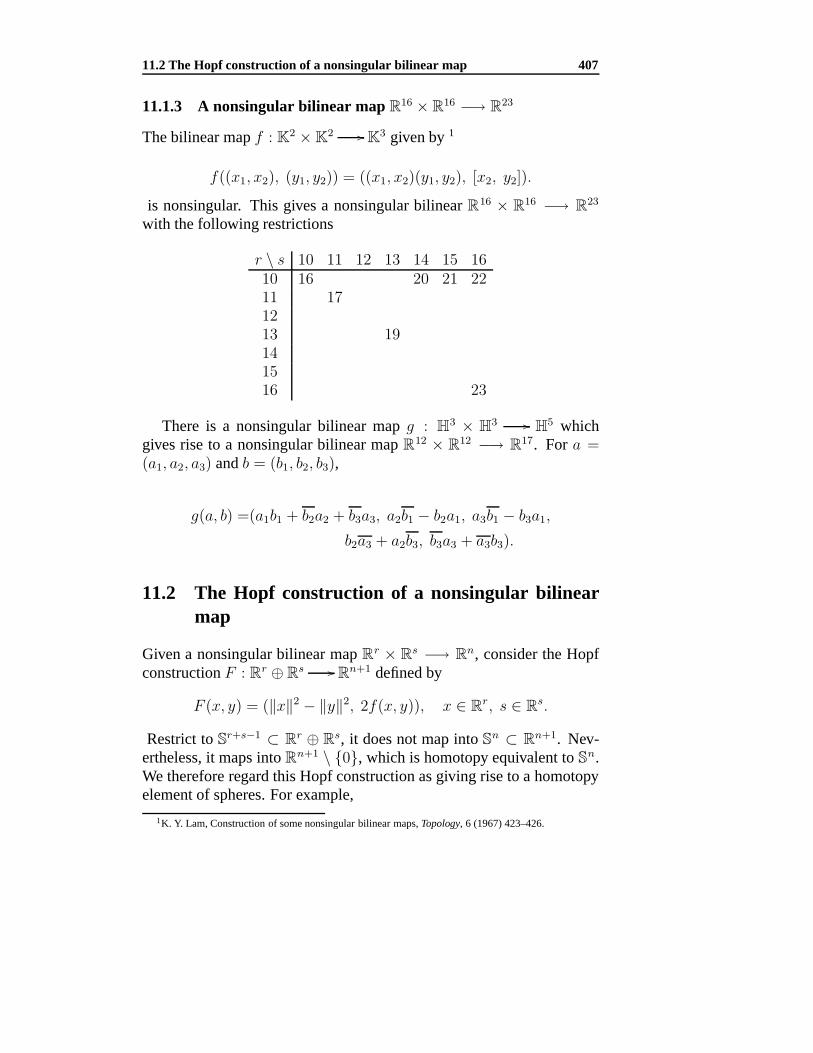
11.1.3 A nonsingular bilinear map R16 × R16 −→ R23
The bilinear map f : K2 × K
2 K3 given by 1
f((x1, x2), (y1, y2)) = ((x1, x2)(y1, y2), [x2, y2]).
is nonsingular. This gives a nonsingular bilinear R16 × R16 −→ R23
with the following restrictions
r \ s 10 11 12 13 14 15 1610 16 20 21 2211 171213 19141516 23
There is a nonsingular bilinear map g : H3 × H3 H5 whichgives rise to a nonsingular bilinear map R12 × R12 −→ R17. For a =(a1, a2, a3) and b = (b1, b2, b3),
g(a, b) =(a1b1 + b2a2 + b3a3, a2b1 − b2a1, a3b1 − b3a1,
b2a3 + a2b3, b3a3 + a3b3).
11.2 The Hopf construction of a nonsingular bilinearmap
Given a nonsingular bilinear map Rr × Rs −→ Rn, consider the Hopfconstruction F : R
r ⊕ Rs Rn+1 defined by
F (x, y) = (‖x‖2 − ‖y‖2, 2f(x, y)), x ∈ Rr, s ∈ R
s.
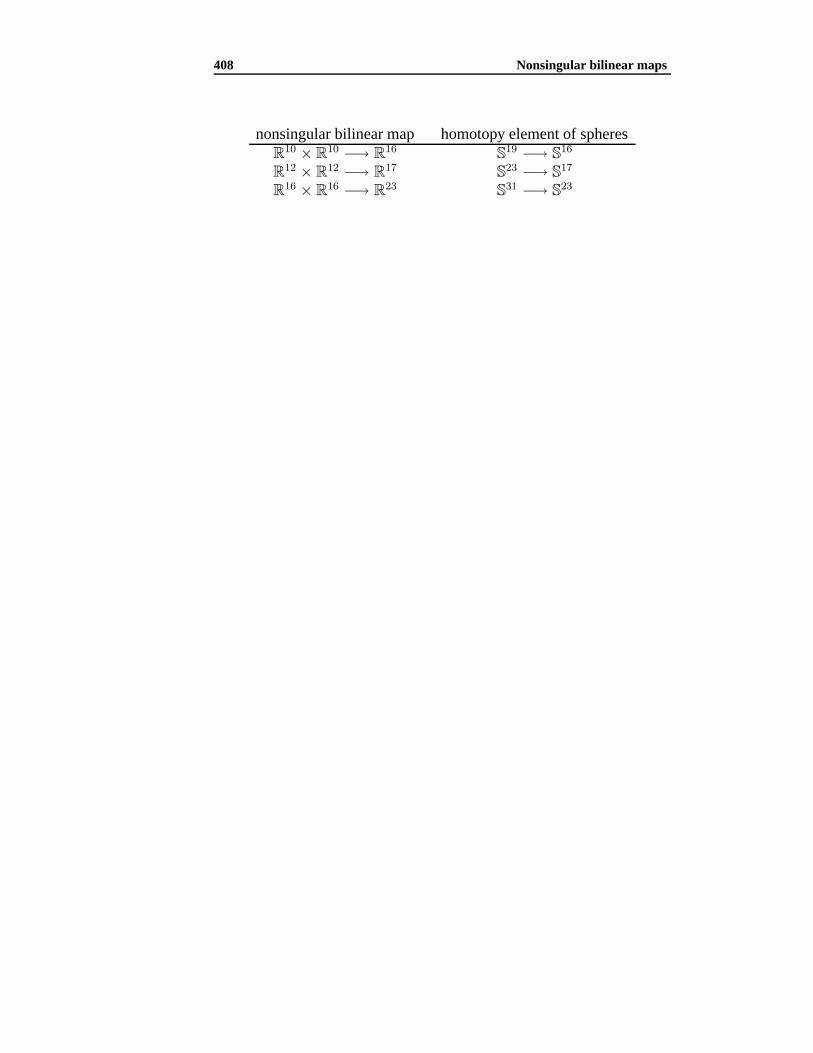
Restrict to Sr+s−1 ⊂ Rr ⊕ Rs, it does not map into Sn ⊂ Rn+1. Nev-ertheless, it maps into Rn+1 \ 0, which is homotopy equivalent to Sn.We therefore regard this Hopf construction as giving rise to a homotopyelement of spheres. For example,
1K. Y. Lam, Construction of some nonsingular bilinear maps, Topology, 6 (1967) 423–426.
408 Nonsingular bilinear maps
nonsingular bilinear map homotopy element of spheresR
10 × R10 −→ R
16S
19 −→ S16
R12 × R12 −→ R17 S23 −→ S17
R16 × R16 −→ R23 S31 −→ S23
Chapter 12
Quadratic forms betweeneuclidean spheres
12.1 Quadratic forms between euclidean spaces
A quadratic form between euclidean spaces is a map g : Rm Rn
whose components are homogeneous quadratic functions (of coordinatesof points in the domain). Associated with a quadratic form is a symmet-ric bilinear map B : Rm × Rm Rn satisfying
g(av + bv′) = a2g(v) + b2g(v′) + 2abB(v, v′).
As a smooth map, g has differentials dgx : Rm Rn given by
dgx(y) = 2B(x, y).
12.2 Quadratic forms between euclidean spheres
A map f : Sm −→ Sn is quadratic if it is the restriction of a homoge-neous quadratic map F : R
m+1 Rn+1. Consider two orthogonal unitvectors v, v′ ∈ Sm ⊂ Rm+1.(1) If F (v) = F (v′) = q, then F maps the great circle through v and v ′
to the point q ∈ Sn.(2) If F (v) = F (v′), then F “wraps” the great circle through v and
v′ uniformly twice around a circle on Sn which has F (v) and F (v′) asendpoints of a diameter. This follows from
410 Quadratic forms between euclidean spheres
F (cos θ · v + sin θ · v′)− F (v) + F (v′)2
=F (v)− F (v′)
2· cos 2θ +B(v, v′) · sin 2θ.
Proposition 12.1. If F : Sm −→ S
n is a homogeneous quadratic map,then for every q ∈ Sn, the inverse image F−1(q) is a great sphere in Sm,being the intersection of Sm with a linear subspace
Wq = ker(B∗v Bv − 4pv) ⊂ R
m+1, v ∈ F−1(q).
12.3 Hidden normed bilinear maps
Consider a quadratic form F : Sm Sn with associated bilinear mapB : Rm+1 × Rm+1 −→ Rn+1. We show that corresponding to everypoint q ∈ Im F , there is a restriction of B to a nonsingular bilinearmap, whose Hopf construction represents the same homotopy class ofspheres as F does. Furthermore, this nonsingular bilinear map ‘hidden’at q can be deformed in a canonical way, via nonsingular bilinear maps,into a normed bilinear map, so that we can actually speak of the ‘normedbilinear map hidden at’ q.
Proposition 12.2. For any q ∈ Sn in the image of F , the restriction ofB to
Bq : Wq ×W⊥q −→ τq(S
n)
is a nonsingular bilinear map.
Proof. The bilinearity of Bq is clear. Let v be a unit vector in Wq and v′ aunit vector in W⊥
q . By Corollary 1.4, Bq(v, v′) = B(v, v′) is orthogonal
to q. This vector cannot be zero, for otherwise, F (v ′) = f(v) and v′ ∈Wq, a contradiction. This shows that Bq is nonsingular.
We call this the nonsingular bilinear map hidden (inside the quadraticform F ) at the point q ∈ S
n. The Hopf construction of this map can bedeformed, by normalization, into a map between spheres, and hence rep-resents a homotopy element of spheres. We show that this must representthe same homotopy class of the quadratic form F . Bypassing details ofnormalizations, it is enough to prove
12.3 Hidden normed bilinear maps 411
Proposition 12.3. Let q be a point in the image of F . There is a homo-topy Ht : S(V1) V2 \ 0 such that H0 = F (regarded as a map intoV2 \ 0) and H1 = the Hopf construction of Bq with poles ±q.
Proof. The hidden nonsingular bilinear map Bq is given by
Bq(v, v′) =
1
2(F (v + v′)− F (v′)− ‖v‖2q).
The Hopf construction of this map with poles ±q is the map Fq : Sm =S(Wq ⊕W⊥
q ) −→ Rn+1 given by
Fq(v, v′) = (‖v‖2 − ‖v′‖2)q + 2Bq(v, v
′)= F (v + v′)− F (v′)− ‖v′‖2q.
Define a homotopy Ht : Sm Rn+1, 0 ≤ t ≤ 1, by
Ht(v, v′) = F (v + v′)− tF (v′)− t‖v′‖2q.
Note that Ht(v, v′) = 0 for any t ∈ [0, 1]. To see this, observe that
Ht(v, v′) = 0 implies
2B(v, v′) + (1− t)F (v′) + (‖v‖2 − t‖v′‖2)q = 0.
Since, by Corollary 1.3, B(v, v′) is orthogonal to both q and F (v ′), sucha linear dependence is impossible unless v = 0 and v ′ = 0. Thus, eachHt, t ∈ [0, 1], maps into V2 \ 0, and the proposition follows by notingthat H0 = F and H1 = Fq.
Remark. In fact, the proof above can be slightly modified to show thatthe homotopy Ht takes place in the orthogonal complement of q.
Let f : Rr × Rs −→ Rn be a bilinear map. For each x ∈ Rr,let fx : Rs Rn denote the linear map induced by f . Suppose f isnonsingular. Then, for each nonzero x ∈ R
r,(i) the linear map fx is injective;(ii) the endomorphism gx := f ∗
x fx is self - adjoint, and has positiveeigenvalues;(iii) y ∈ Rs is an eigenvector of gx = f ∗
x fx corresponding to aneigenvalue λ if and only if
〈f(x, y), f(x, y′)〉 = λ〈y, y′〉for every y′ ∈ Rs;(iv) if y1, . . . , ys are orthogonal unit eigenvectors of gx, then f(x, y1), . . . , f(x, ys)are mutually orthogonal in Rn.
412 Quadratic forms between euclidean spheres
Lemma 12.4. Let f : Rr × Rs −→ Rn be a nonsingular bilinear map.Suppose the endomorphism gx is independent of x ∈ S
r−1. Then, fcan be homotoped via nonsingular bilinear maps into a normed bilinearmap.
Proof. Let E = (ε1, . . . , εs) be an orthonormal basis of (common) uniteigenvectors of gx with positive eigenvalues λ1, . . . , λs. Take an or-thonormal basis E = (e1, . . . , er) of X and tabulate the bilinear mapf by the matrix Mf := (f(ei, εj)). Note that by the choice of the basisE of Y , for each i = 1, . . . , r, the vectors f(ei, εj), j = 1, . . . , s aremutually orthogonal.
For each t ∈ [0, 1], let Mt be the matrix
Mt =
(1√
1− t+ tλj
f(ei, εj)
).
This tabulates a bilinear map ft : X × Y Z which is nonsingular,since every induced linear map ft,x : Y Z, x ∈ X , is injective, beinggiven by
ft,x(εj) =1√
1− t+ λj
f(x, εj), 1 ≤ j ≤ s,
and extension by linearity. The family ft, 0 ≤ t ≤ 1, is, therefore, ahomotopy of nonsingular bilinear maps. Furthermore,
‖f1,x(εj)‖ = ‖ 1√λj
f(x, εj)‖ = 1, 1 ≤ j ≤ s.
Thus, M1 tabulates a normed bilinear map, and is obtained simply bynormalizing each vector in the matrix M0 = Mf .
Proposition 12.5. Every hidden nonsingular bilinear map of a quadraticform between spheres can be homotoped via nonsingular bilinear mapsinto a normed bilinear map.
Proof. For any q in the image of F , choose an orthonormal basis w1, . . . , wm+1−k
of W⊥q . By Proposition 2.3,
〈Bq(v, wi, Bq(wj)〉 = 〈B∗v Bv(wi), wj〉 = 1
2(〈wi, wj〉−〈q, B(wi, wj)〉
is independent of the choice of v ∈ F−1(q) = S(Wq). The result nowfollows from ?.
12.4 The hidden normed bilinear maps of a monomial bilinear map 413
We call the normed bilinear map obtained by effecting the above ho-motopy to the nonsingular bilinear map Bq the normed bilinear map Bq
hidden at q. We shall find a simple description of this map in the nextsection. We summarize the results in the present section by
Theorem 12.6. Let F : Sm Sn be a nonconstant quadratic form. Foreach point q in the image of F , there is a hidden normed bilinear map oftype [k,m− k + 1, n], m− n+ 1 ≤ k = dimWq ≤ n, representing thesame homotopy class of F .
12.4 The hidden normed bilinear maps of a monomialbilinear map
Let f : Rr × Rs −→ Rn be a monomial normed bilinear map, withrespect to orthonormal bases e1, . . . , er or Rr, ε1, . . . , εs of Rs, and c1,. . . , cn of Rn. This means that each f(ei, εj) = ck for some k. Let c beone of these. The hidden normed bilinear at c can easily found from atabulation of f . Suppose
f(e1, ε1) = · · · = f(ek, εk) = c,
and f is tabulated by the matrix(A BC D
).
Then the normed bilinear map hidden at c is the one tabulated by(A B Ct
).
12.5 Appendix: An application
We consider the problem of mapping a euclidean sphere of given dimen-sion via a quadratic form into one of lowest possible dimension. Let
q(m) := minn : ∃ nonconstant quadratic form Sm −→ S
n.Analogously, we also consider
p(n) := maxm : ∃ nonconstant quadratic form Sm −→ S
n.
414 Quadratic forms between euclidean spheres
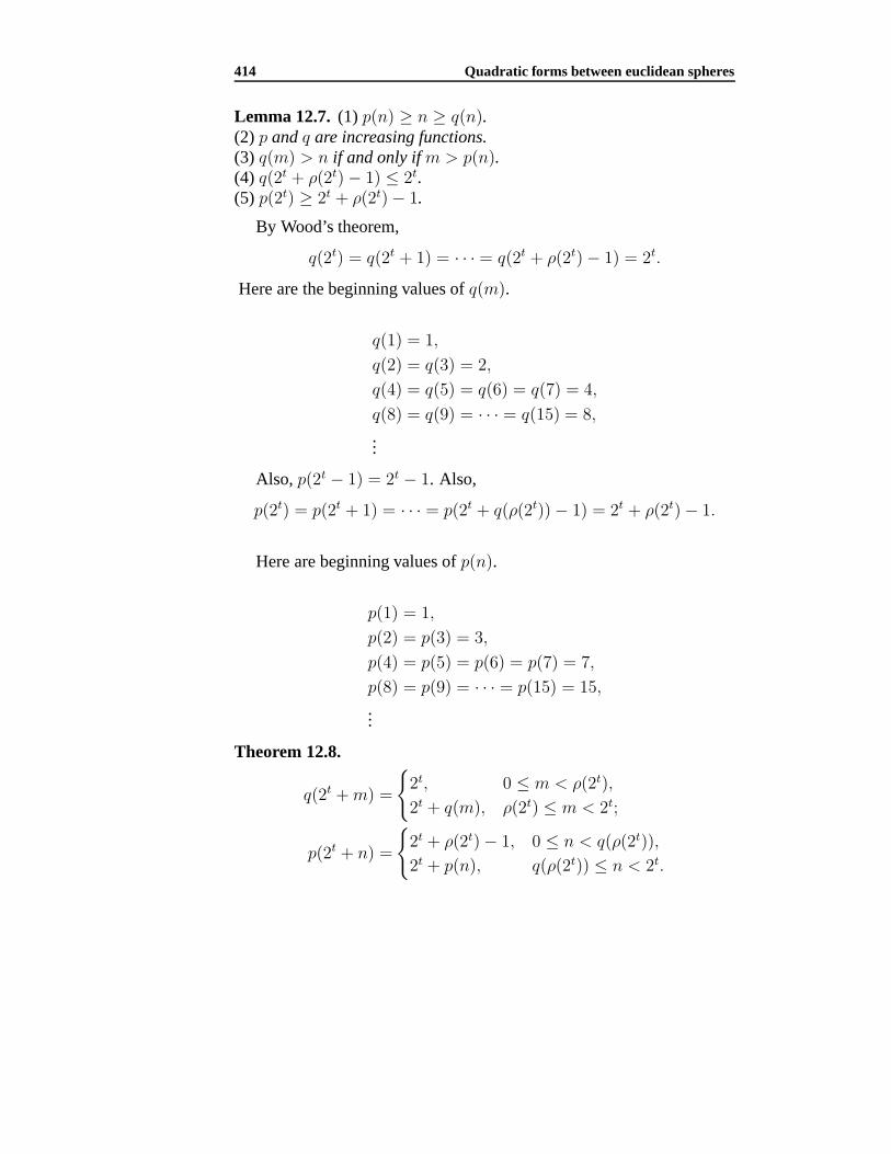
Lemma 12.7. (1) p(n) ≥ n ≥ q(n).(2) p and q are increasing functions.(3) q(m) > n if and only if m > p(n).(4) q(2t + ρ(2t)− 1) ≤ 2t.(5) p(2t) ≥ 2t + ρ(2t)− 1.
By Wood’s theorem,
q(2t) = q(2t + 1) = · · · = q(2t + ρ(2t)− 1) = 2t.
Here are the beginning values of q(m).
q(1) = 1,
q(2) = q(3) = 2,
q(4) = q(5) = q(6) = q(7) = 4,
q(8) = q(9) = · · · = q(15) = 8,
...
Also, p(2t − 1) = 2t − 1. Also,
p(2t) = p(2t + 1) = · · · = p(2t + q(ρ(2t))− 1) = 2t + ρ(2t)− 1.
Here are beginning values of p(n).
p(1) = 1,
p(2) = p(3) = 3,
p(4) = p(5) = p(6) = p(7) = 7,
p(8) = p(9) = · · · = p(15) = 15,
...
Theorem 12.8.
q(2t +m) =
2t, 0 ≤ m < ρ(2t),
2t + q(m), ρ(2t) ≤ m < 2t;
p(2t + n) =
2t + ρ(2t)− 1, 0 ≤ n < q(ρ(2t)),
2t + p(n), q(ρ(2t)) ≤ n < 2t.
12.5 Appendix: An application 415
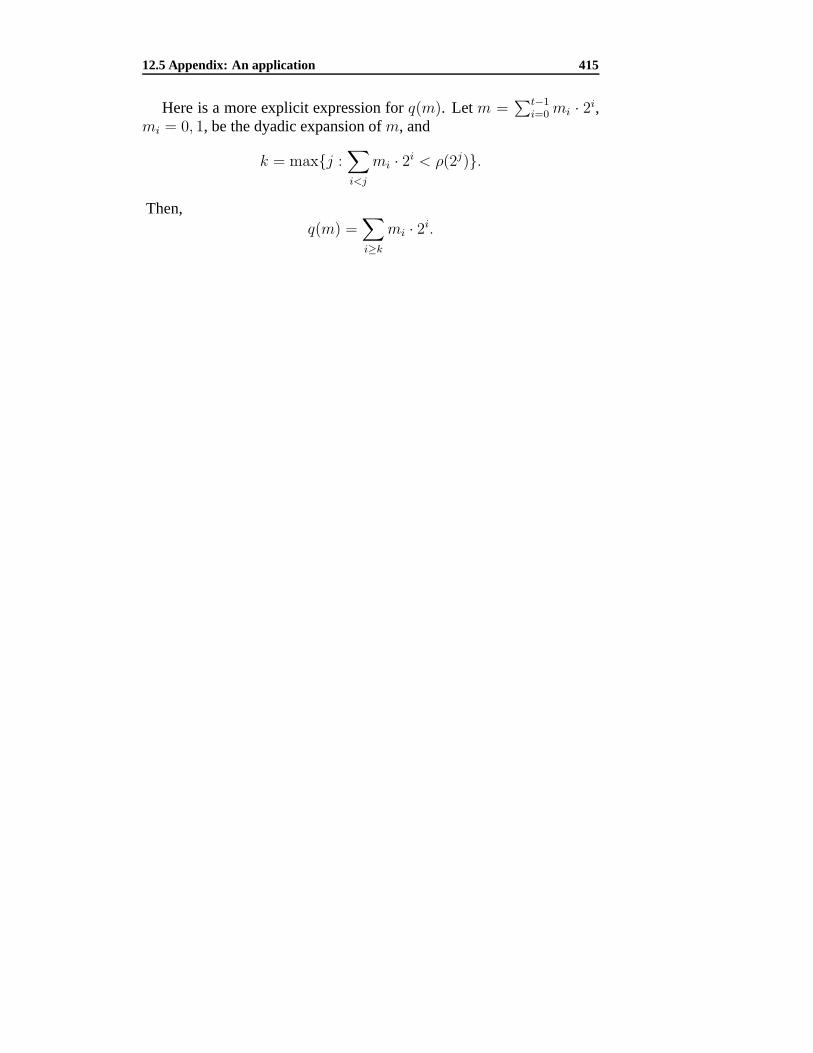
Here is a more explicit expression for q(m). Let m =∑t−1
i=0 mi · 2i,mi = 0, 1, be the dyadic expansion of m, and
k = maxj :∑i<j
mi · 2i < ρ(2j).
Then,q(m) =
∑i≥k
mi · 2i.
Chapter 13
Spaces of similarities
13.1 The space Hom(Rs,Rn) of linear maps
The space of linear maps Hom(Rs,Rn) has dimension sn. It has a basisµi,j : Rs Rn, 1 ≤ i ≤ s, 1 ≤ j ≤ n defined by
µi,j(ek) = δi,kej , 1 ≤ k ≤ s.
We endow it with an inner product by taking µi,j, 1 ≤ i ≤ s, 1 ≤ j ≤ nas an orthonormal basis. Thus, if we represent linear maps Rs Rn
by s×n matrices, the space of matrices Ms,n has an inner product givenby
〈A, B〉 = 1
s· Tr(ABt).
13.1.1 Similarities
A linear map τ : Rs Rn is a similarity if there exists a(τ) ∈ R suchthat
〈τ(y), τ(y′)〉 = a(τ)〈y, y′〉for all y, y′ ∈ Rn. a(τ) is called the similarity factor of τ . It follows
from the polarization identity
〈u, v〉 = 1
2
(||u+ v||2 − ||u||2 − ||v||2)that τ is a similarity with factor b2 if ||τ(y)|| = b||y|| for every y ∈ Rn.
An isometry is a similarity with factor 1.
502 Spaces of similarities
A linear map τ : Rs Rn has a dual τ ∗ : Rn Rs defined by
〈x, τ ∗(y)〉 = 〈τ(x), y〉, x ∈ Rs, y ∈ R
n.
τ ∈ Hom(Rs,Rn) is a similarity if and only if τ ∗ τ = kι for somek ∈ R.
Let τ : Rs Rn be a similarity with factor k represented by an s×nmatrix A. The matrix A satisfies AAt = kIs, and is called a similaritymatrix.
13.2 Spaces of similarities and normed bilinear maps
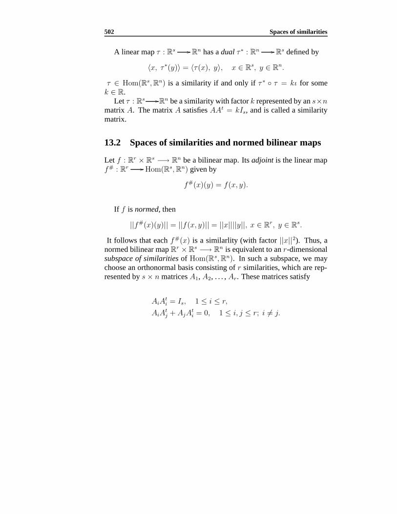
Let f : Rr × Rs −→ Rn be a bilinear map. Its adjoint is the linear mapf# : R
r Hom(Rs,Rn) given by
f#(x)(y) = f(x, y).
If f is normed, then
||f#(x)(y)|| = ||f(x, y)|| = ||x||||y||, x ∈ Rr, y ∈ R
s.
It follows that each f#(x) is a similarlity (with factor ||x||2). Thus, anormed bilinear map Rr × Rs −→ Rn is equivalent to an r-dimensionalsubspace of similarities of Hom(Rs,Rn). In such a subspace, we maychoose an orthonormal basis consisting of r similarities, which are rep-resented by s× n matrices A1, A2, . . . , Ar. These matrices satisfy
AiAti = Is, 1 ≤ i ≤ r,
AiAtj + AjA
ti = 0, 1 ≤ i, j ≤ r; i = j.
Chapter 14
Isoclinic n-planes in R2n
14.1 Angles between two n-planes in R2n
Consider R2n = Rn ⊕ Rn, and write elements of R2n as (x, y) withx, y ∈ Rn. Let O be the n-plane y = 0, and O⊥ the one with equationx = 0. An n-plane A can be represented by an equation y = xA for ann× n matrix A if and only if A ∩ O⊥ = 0.
Consider two n-planes with equations A : y = xA and B : y = xBfor n × n matrices A and B. The orthogonal projection of a vector(u, uA) ∈ A in the n-plane B is the vector (v, vB) with
v = u(I + ABt)(I +BBt)−1.
Consequently, the angle θ(u) between (u, uA) ∈ A and its orthogonalprojection in B is given by
cos2 θ = f(u) :=uPut
uQut,
where P = (I+ABt)(I+BBt)−1(I+BAt) and Q = I+AAt. There aren critical values of f(u), which are the roots of the polynomial equation
det(P − λQ) = 0.
The corresponding values of θ ∈ [0, π2
]are the angles between the two
n-planes A and B.The two n-planes are said to be isoclinic if these angles are all equal
to θ, equivalently, P = λQ for λ = cos2 θ.
504 Isoclinic n-planes in R2n
14.2 Maximal sets of isoclinic n-planes in R2n
Consider a set of mutually isoclinic n-planes in R2n. Without loss of
generality we consider one of these to be O. The n-plane O⊥ is clearlyisoclinic to O, and every n-plane isoclinic to O is also isoclinic to O⊥.Let A : y = xA be one such n-plane, then
The only n-plane isoclinic to O that cannot be written in the formy = xA is O⊥. The matrix A satisfies AAt = σI for some σ ∈ R, i.e., Ais a similarity matrix.
Let A : y = xA and B : y = xB be both isoclinic to O. ThenAAt = λ1I and BBt = λ2I for λ1, λ2 ∈ R. The n-planes A and B arethemselves isoclinic if and only if (A + B)(A + B)t = λI for some λ.Equivalently, every linear combination of A and B is a similarity matrix.
Theorem 14.1 (Wong). A maximal set of mutually isoclinic n-planes inR2n is equivalent to a subspace of similarities of Rn.
Chapter 15
Hurwitz-Radon Theorem
15.1 Normed bilinear maps and systems of anticom-muting skew symmetric matrices
A normed bilinear map f : Rr × Rn −→ Rn is equivalent to a subspaceof similarities (in the euclidean space of linear transformations) of R
n.For a given integer n, we determine the largest possible dimension of asubspace of similarities of Hom(Rn,Rn).
Let V be an r-dimensional subspace of similarities of Rn. A familyf1, . . . , fr ∈ Hom(Rn,Rn) form an orthonormal basis of V if and onlyif
f ∗i fi = ι, 1 ≤ i ≤ r,
f ∗i fj + f ∗
j fi = 0, 1 ≤ i, j ≤ r, i = j.
If ι ∈ V , and τ1 = ι, τ2, . . . , τr form an orthonormal basis of V , then
τ ∗i =− τi, 2 ≤ i ≤ r,
τ 2 =− ι, 2 ≤ i ≤ r,
τiτj =− τjτi, i = j, 2 ≤ i, j ≤ r.
Therefore, a normed bilinear map Rr × Rn −→ Rn is equivalent toa system of r − 1 mutually anticommutating skew symmetric matrices(of order n) each squaring to −In. We determine the Hurwitz-Radonfunction
ρ(n) := maxr : ∃ normed bilinear map Rr × R
n −→ Rn.
506 Hurwitz-Radon Theorem
15.2 (r, s)-families of similarities
Two subspaces V , W of similarities are said to be amicable if τ ∗ ϕ =ϕ∗ τ for τ ∈ V and ϕ ∈ W .
Lemma 15.1. If V and W are amicable and have orthonormal basesι, τ2, . . . , τr for V andϕ1, . . . , ϕs for W , then(i) τ2, . . . , τr are skew and τ 2
i = −ι for 2 ≤ i ≤ r;(ii) ϕ1, . . . , ϕs are symmetric, and ϕ2 = ι for 1 ≤ j ≤ s;(iii) τ2, . . . , τr, ϕ1, . . . , ϕs mutually anticommute.
We shall call a collection of isometries
ι, τ2, . . . , τr; ϕ1, . . . , ϕs
satisfying these conditions an (r, s)-family (of isometries on Rn).
Lemma 15.2. (a) If τ : Rn Rn is a linear map satisfying τ 2 = −ι,then n must be even.
(b) If τ2, τ3 : Rn Rn are anticommuting linear maps satisfyingτ 22 = τ 2
3 = −ι, then n must be divisible by 4.
Proof. (a) Let V+ := x + τ(x) : x ∈ Rn and V− := x − τ(x) : x ∈
Rn. It is easy to check that τ maps V+ into V− and V− into V+. Sinceτ 2 = −ι, the composites V+
V− V+ and V− V+ V− are
both −ι. This shows that V+ and V− are isomorphic. Since V+ ⊕ V− =Rn, n must be even. 1
(b) Let V+ := x+τ2(x) : x ∈ Rn and V− := x−τ2(x) : x ∈ Rn.From (a), τ2 interchanges V+ and V−. It is easy to check that τ3 alsointerchanges V+ and V−. It follows that τ := τ2τ3 is an endomorphismon V+. Note that τ = τ1τ2 satisfies τ 2 = −ι. This means that dim V+ iseven, and n must be divisible by 4.
Lemma 15.3 (Construction lemma). Given an (r, s)-family
ι, τ2, . . . , τr; ϕ1, . . . , ϕs
1Alternatively, the determinant of an odd order skew symmetric matrix is zero.
15.2 (r, s)-families of similarities 507
on Rn, there is an (r + 1, s+ 1)-family on R2n(ι
ι
),
(τ2
τ2
), . . . ,
(τr
τr
),
( −ιι
);(
ϕ1
ϕ1
), . . . . . . ,
(ϕs
ϕs
),
(ι
ι
).
Lemma 15.4 (Subspace lemma). If there is an (r, s)-family on Rn withr ≥ 2, s ≥ 1, then n is even, say n = 2m, and there is an (r−1, s−1)-family on Rm.
Lemma 15.5 (Shift lemma). Suppose there is an (r, s)-family on Rn.If r > 4, then there is an (r − 4, s+ 4)-family on Rn,If s ≥ 4, then there is an (r + 4, s− 4)-family on Rn.
Lemma 15.6 (Expansion lemma). Suppose there is an (r, s)-family onRn.If r− s ≡ 3 mod 4, then this can be expanded into an (r + 1, s)-familyon Rn,If r − s ≡ 1 mod 4, then this can be expanded into an (r, s+ 1)-familyon Rn.
Lemma 15.7 (Reduction lemma). If ρ(n) ≥ 9, then n is divisible by16, and ρ
(n16
) ≥ ρ(n)− 8.
Proposition 15.8 (Upper bound theorem). Let n = 2t(2c+ 1).(a) ρ(n) ≤ 2t+ 2.(b) The maximum possible value of r + s for an (r, s)-family on Rn is2t+ 2.
15.2.1 Proof of subspace lemma
Letι, τ2, . . . , τr; ϕ1, . . . , ϕs
be an (r, s)-family on Rn. Consider h := τrϕs. Note that(i) h2 = ι,(ii) hτr = −τrh, and(iii) h commutes with each of τ2, . . . , τr−1, ϕ1, . . . , ϕs−1. From (i), thereis an orthogonal decomposition
Rn = V+ ⊕ V−,
508 Hurwitz-Radon Theorem
where
V+ := x+ h(x) : x ∈ Rn,
V− := x− h(x) : x ∈ Rn.
In fact, V+ and V− are respectively the eigenspaces of h correspondingto the eigenvalues +1 and −1. We show that τr interchanges V+ and V−.For x ∈ V+,
τr(x) = τr(h(x)) = −hτr(x).
Therefore, τr(x) ∈ V−. Similarly, τr(x) ∈ V+ for x ∈ V−. It followsthat dimV+ = dimV−, and n must be even. We write n = 2m.
From (iii), each of τ2, . . . , τr−1, and ϕ1, . . . , ϕs−1 preserves V+ (andV−). Identifying V+ with Rm, we have an (r − 1, s− 1)-family on Rm.
15.2.2 Proof of shift and expansion lemmas
Let A be a noncommutative ring with unit. Consider in A distinct pair-wise anticommuting elements a1, . . . , ah. Put a = a1 · · ·ah.
(1) a anticommutes with each of a1, . . . , ah if and only if h is even.(2) Suppose ai = ε = ±1. Then a2 = (−1)
12h(h−ε). In other words,
(i) if each a2i = −1, then
a2 =
1, h ≡ 0, 3 mod 4,
−1, h ≡ 1, 2 mod 4;
(ii) if each a2i = 1, then
a2 =
1, h ≡ 0, 1 mod 4,
−1, h ≡ 2, 3 mod 4.
(3) If a1, a2, a3, a4 are anticommuting elements of A and a = a1a2a3a4.Put a′i = aai for i = 1, 2, 3, 4. Then a′1, a′2, a′3, a′4 are anticommuting,and each a′i
2 = −1 if and only if each a2i = 1.
(4) Suppose a1, . . . , ah and b1, . . . , bk are all distinct and mutuallyanticommute. Let a = a1 · · ·ah and b = b1 · · · bk. Then ab = (−1)hkba.
15.2.3 Proof of shift lemma
Letι, τ2, . . . , τr; ϕ1, . . . , ϕs

15.2 (r, s)-families of similarities 509
be an (r, s)-family on Rn. If r > 4, let τ = τr−3τr−2τr−1τr, and
ϕs+1 = ττr−3, ϕs+2 = ττr−2, ϕs+3 = ττr−1, ϕs+4 = ττr.
We have an (r − 4, s+ 4)-family
ι, τ2, . . . , τr−4; ϕ1, . . . , ϕs, ϕs+1, ϕs+2, ϕs+3, ϕs+4.
The proof for an (r + 4, s− 4)-family given s ≥ 4 is similar.
15.2.4 Proof of expansion lemma
Letι, τ2, . . . , τr; ϕ1, . . . , ϕs
be an (r, s)-family on Rn. Consider
z = τ2 · · · τrϕ1 · · ·ϕs.
Note that this contains r + s − 1 factors. By (1), z anticommutes witheach of τ2, . . . , τr, ϕ1, . . . , ϕs if and only if r + s− 1 is even. Write
τ = τ2 · · · τr, ϕ = ϕ1 · · ·ϕs.
Note that
z2 =(τϕ)2
=(−1)(r−1)sτ 2ϕ2
=(−1)(r−1)s+ 12(r−1)r+ 1
2s(s−1)ι
=(−1)12(r+s−1)2+ 1
2(r−s−1)ι.
Assuming r + s− 1 even, we easily see that
z2 =
ι, if r − s− 1 ≡ 0 mod 4,
−ι, if r − s− 1 ≡ 2 mod 4.
Therefore, we obtain an (r + 1, s)-family
ι, τ2, . . . , τr, z; ϕ1, . . . , ϕs
if r − s ≡ −1 mod 4, and an (r, s+ 1)-family
ι, τ2, . . . , τr; z, ϕ1, . . . , ϕs
if r − s ≡ 1 mod 4.
510 Hurwitz-Radon Theorem
15.2.5 Proof of reduction lemma
Let r ≥ 9 and there be an (r, 0)-family on Rn.
(r, 0)− family on Rn
⇒(r − 4, 4)− family on Rn
⇒(r − 8, 0)− family on Rn16
15.2.6 Proof of upper bound theorem
(a) For t ≥ 4, ρ(2t(2c+1)) ≥ 2t+3 ⇒ ρ(2t−4(2c+1)) ≥ 2(t− 4)+ 3by the reduction lemma. We need only consider t ≤ e3. For t = 0, 1,this follows from Lemma 15.2. In fact, ρ(2(2c+ 1)) ≤ 2.
For t = 2, if ρ(4(2c + 1)) ≥ 7, we have by restriction a (5, 0)-family. By the expansion lemma, there is a (5, 1)-family on R
4(2c+1). Bythe subspace lemma, there is a (4, 0)-family on R2(2c+1), contradictingρ(2(2c+ 1)) ≤ 2.
For Tt = 3, if ρ(8(2c+ 1)) ≥ 9, we have a (9, 0)-family on R8(2c+1).By the expansion lemma, there is a (9, 1)-family. By the subspace lemma,there is a (8, 0) family on R4(2c+1), contradicting ρ(4(2c+ 1)) ≤ 6.
(b) Beginning with a (2, 2)-family on R2,(1
1
),
( −11
);
(1
1
),
(1
−1
),
on R2, we easily construct a (t + 1, t + 1)-family on R2t, and so on
R2t(2c+1).To show that r+ s ≤ 2t+2 we use induction. This is clearly true for
t = 1, and for n = 2(2c+ 1) more generally.Suppose there is an (r, s)-family on R
n with r + s = 2t+ 3. By (a),r ≤ 2t + 2. It follows that s ≥ 1, and r ≥ 2. By the subspace lemmathere is an (r − 1, s − 1)-family on R2t−1(2c+1) with (r − 1) + (s −1) = 2(t − 1) + 3. Continuing, we obtain an (r, s)-family on R2(2c+1)
with r + s = 5. This is a contradiction since r ≤ 2. If r = 1, froma (1, 4)-family, we obtain a (5, 0)-family, an impossibility by the shiftlemma. If r = 2, from a (2, 3)-family, we obtain a (1, 2)-family onR2c+1. This is an impossibility since the existence of anticommuting ϕ1
and ϕ2 satisfying ϕ21 = ϕ2
2 = ι requires the dimension to be even.
15.3 Hurwitz-Radon theorem 511
15.3 Hurwitz-Radon theorem
Theorem 15.9 (Hurwitz-Radon). For a given integer n = 2t(2c + 1),the largest possible value of r for which there exists a normed bilinearmap Rr × Rn −→ Rn is
ρ(n) =
2t+ 1, t ≡ 0 mod 4,
2t, t ≡ 1, 2 mod 4,
2t+ 2, t ≡ 3 mod 4.
Proof. By the upper bound theorem (Proposition 15.8) ρ(n) ≤ 2t + 2.Indeed, if an (r, 0)-family on Rn is extended to an (r, s)-family for somes, r + s ≤ 2t+ 2. Note that there is a (t+ 1, t + 1)-family on Rn. Weexamine 4 cases.
t ≡ 3 mod 4
If t ≡ 3 mod 4, by the shift lemma, there is a (2t+ 2, 0)-family on Rn.Therefore, there is a (2t+ 2, 0)-family, and
ρ(n) = 2t+ 2 if t ≡ 3 mod 4.
t ≡ 0 mod 4
By the shift lemma, there is a (2t + 1, 1)-family on Rn. We claim thatρ(n) = 2t + 1, for if ρ(n) ≥ 2t + 2, then by the reduction lemma,ρ(2c+ 1) = ρ
(n2t
) ≥ 2, a contradiction.
t ≡ 1 mod 4
By the shift lemma, there is a (2t, 2)-family on Rn. We claim that ρ(n) =
2t, for if ρ(n) ≥ 2t + 1, then by the reduction lemma, ρ(2(2c + 1)) =ρ(
n2t−1
) ≥ (2t+ 1)− (2t− 2) = 3, a contradiction.
t ≡ 2 mod 4
We need only consider t > 4. By the shift lemma, there is a (2t− 1, 3)-family. By restriction we have a (2t− 1, 0)-family. Since (2t− 1)− 0 ≡3 mod 4, by the expansion lemma, we can extend this to a (2t, 0)-family.
512 Hurwitz-Radon Theorem
We claim that ρ(n) = 2t, for if ρ(n) ≥ 2t + 1, then by the reductionlemma, ρ(4(2c+1)) = ρ
(n
2t−2
) ≥ (2t+1)−2(t−2) = 5, a contradiction.
Chapter 16
Fundamental group
16.1 The loop space Ω(X, x0) and the fundamental groupπ1(X, x0)
Let X be a topological space with a basepoint x0 ∈ X . The space ofpaths in X emanating from x0 is the space
P (X, x0) := ω ∈ XI : ω(0) = x0.The space of loops based at x0 is the subspace
Ω(X, x0) := ω ∈ XI : ω(0) = ω(1) = x0.There is a natural addition of loops: for ω1, ω2 ∈ Ω(X, x0), their con-
catenation ω1 · ω2 = ω is given by
ω(t) =
ω1(2t), 0 ≤ t ≤ 1
2,
ω2(2t− 1), 12≤ t ≤ 1.
Two loops ω0 and ω1 are homotopic if there is a path in Ω(X, x0)connecting ω0 to ω1, i.e., a homotopy H : I × I X satisfying
H(t, 0) = ω0(t), H(t, 1) = ω1(t);H(0, s) = x0, H(1, s) = x0.
The set of homotopy classes of loops in X with basepoint x0 is de-noted by π1(X, x0). The following proposition justifies calling this thefundamental group of X (with basepoint x0).
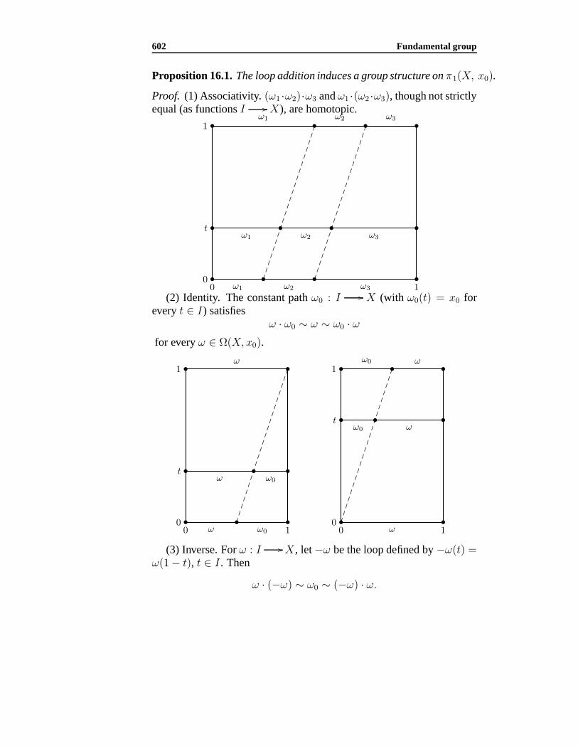
602 Fundamental group
Proposition 16.1. The loop addition induces a group structure on π1(X, x0).
Proof. (1) Associativity. (ω1 ·ω2)·ω3 and ω1 ·(ω2 ·ω3), though not strictlyequal (as functions I X), are homotopic.
ω1 ω2 ω3
ω1 ω2 ω3
ω1 ω2 ω3
0
t
1
0 1(2) Identity. The constant path ω0 : I X (with ω0(t) = x0 for
every t ∈ I) satisfiesω · ω0 ∼ ω ∼ ω0 · ω
for every ω ∈ Ω(X, x0).
ω ω0
ω
ω ω0
0
t
1
0 1 ω
ω0 ω
ω0 ω
0
t
1
0 1
(3) Inverse. For ω : I X , let −ω be the loop defined by −ω(t) =ω(1− t), t ∈ I . Then
ω · (−ω) ∼ ω0 ∼ (−ω) · ω.
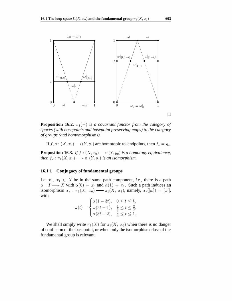
16.1 The loop space Ω(X, x0) and the fundamental group π1(X, x0) 603
ω0 = ω|1
ω −ω
ω|[0,t]
ω|t
ω|[t,0]
0
t
1
0 1 ω0 = ω|1
−ω ω
ω|[1,1−t]
ω|1−t
ω|[1−t,1]
0
t
1
0 1
Proposition 16.2. π1(−) is a covariant functor from the category ofspaces (with basepoints and basepoint preserving maps) to the categoryof groups (and homomorphisms).
If f, g : (X, x0) (Y, y0) are homotopic rel endpoints, then f∗ = g∗.
Proposition 16.3. If f : (X, x0) (Y, y0) is a homotopy equivalence,then f∗ : π1(X, x0) π1(Y, y0) is an isomorphism.
16.1.1 Conjugacy of fundamental groups
Let x0, x1 ∈ X be in the same path component, i.e., there is a pathα : I X with α(0) = x0 and α(1) = x1. Such a path induces anisomorphism α∗ : π1(X, x0) π1(X, x1), namely, α∗([ω]) = [ω′],with
ω(t) =
α(1− 3t), 0 ≤ t ≤ 1
3,
ω(3t− 1), 13≤ t ≤ 2
3,
α(3t− 2), 23≤ t ≤ 1.
We shall simply write π1(X) for π1(X, x0) when there is no dangerof confusion of the basepoint, or when only the isomorphism class of thefundamental group is relevant.
604 Fundamental group
A connected space X is simply connected if π1(X) = 0. Clearly,a contractible space is simply connected. Also, S
n is simply connectedwhen n ≥ 2.
16.2 The fundamental group of the circle
The first nontrivial example of fundamental group is that of the circle.We take as basepoint of S1 the complex number 1.
Theorem 16.4. π1(S1, 1) is isomorphic to the additive group of integers.
Proof. Consider the exponential map exp : R S1 given by
exp(t) = e2πit, t ∈ R.
Clearly, exp−1(1) = Z.A loop in Ω(S1, 1) is given by a map ω : I S1 satisfying ω(0) =
ω(1) = 1. Such a loop is the image under exp of a unique path ω :I R with initial point ω(0) = 0. Note that ω(1) is an integer, whichwe denote by deg(ω), and call the degree of ω.
(1) deg(ω) depends only on the homotopy class of ω. In other words,if ω′ ∈ Ω(S1, 1) is homotopic to ω rel endpoints, then deg(ω ′) =deg(ω). Therefore we have a function deg : π1(S
1, 1) Z.(2) Clearly, every integer n is equal to deg(ω) for some loop ω in S1.
If n = 0, the path fn : I R given by fn(t) = nt clearly projectsunder exp into a loop in S1 (which winds around the circle n times,counterclockwise or clockwise according as n is positive or negative).If n = 0, we simply take the constant loop. This shows that deg issurjective.
(3) On the other hand, deg is injective. This follows from the fact thatany two paths in R with the same endpoints are homotopic rel endpoints.Therefore, deg : π1(S
1, 1) Z is a bijection.(4) Consider two loops ω1 and ω2 in Ω(S1, 1). If these are “covered”
under exp by paths ω1, ω2 with ω1(1) = m and ω2(1) = n, then the loopω1 ·ω2 is covered by the path which is the “concatenation” of ω1 and ω2:
ω(t) =
ω1(2t), 0 ≤ t ≤ 1
2,
m+ ω2(2t− 1), 12≤ t ≤ 1.
Clearly,
deg([ω1]·[ω2]) = deg([ω1·ω2]) = ω(1) = m+n = deg([ω1])+deg([ω2]).
16.3 Fundamental theorem of algebra 605
This means that deg : π1(S1, 1) Z is a homomorphism. Since deg
is bijective, it is an isomorphism.
16.3 Fundamental theorem of algebra
Theorem 16.5. Every nonconstant polynomial with complex coefficientshas a zero in C.
Proof. We deduce a contradiction by assuming a polynomial
p(z) = zn + a1zn−1 + · · ·+ an−1z + an
without zero. Considered the polynomial as a map p : S1 C − 0.
Write p(z) = zn + f(z). We show that for sufficiently large r > 0, if||z|| = r, zn + tf(z) is nonzero for t ∈ [0, 1]. This follows from
||zn + tf(z)|| >||z||n − t||f(z)||>||z||n − ||f(z)||
>||z||n −n∑
k=1
||akzn−k||
>||z||n −(
n∑k=1
||ak||)||z||n−1 assuming ||z|| > 1
=
(r −
n∑k=1
||ak||)
rn−1,
which is nonzero if we choose r = max(∑n
k=1 ||ak||, 1).Thus, via the homotopy pt : S1 × [0, 1] C−0 given by pt(z) =
(rz)n + tf(rz), the maps z "→ p(rz) and z "→ (rz)n are homotopic.Regarded as a map S1 S1, the latter map clearly has degree n. Thisis a contradiction since the map z "→ p(rz) is homotopic to the constantmap z "→ an via the homotopy z "→ p(trz).

606 Fundamental group
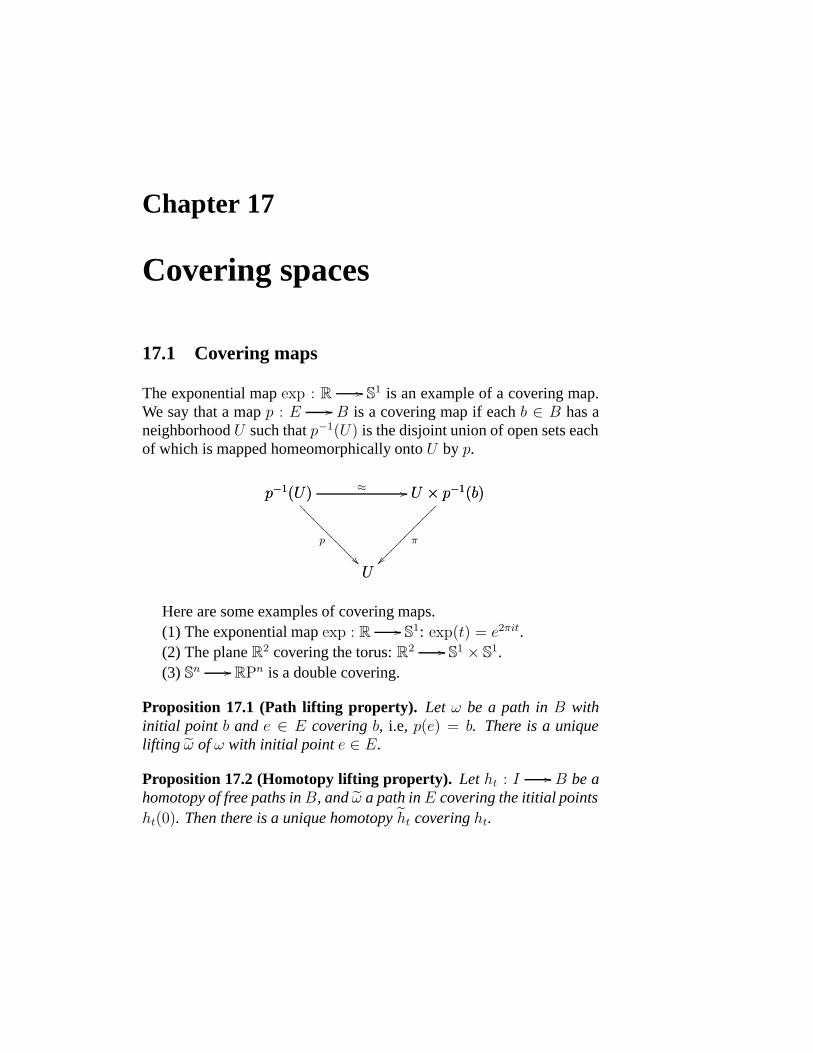
Chapter 17
Covering spaces
17.1 Covering maps
The exponential map exp : R S1 is an example of a covering map.We say that a map p : E B is a covering map if each b ∈ B has aneighborhood U such that p−1(U) is the disjoint union of open sets eachof which is mapped homeomorphically onto U by p.
p−1(U)
U
p
p−1(U) U × p−1(b)≈ U × p−1(b)
U
π
Here are some examples of covering maps.(1) The exponential map exp : R S1: exp(t) = e2πit.(2) The plane R2 covering the torus: R2 S1 × S1.(3) Sn RPn is a double covering.
Proposition 17.1 (Path lifting property). Let ω be a path in B withinitial point b and e ∈ E covering b, i.e, p(e) = b. There is a uniquelifting ω of ω with initial point e ∈ E.
Proposition 17.2 (Homotopy lifting property). Let ht : I B be ahomotopy of free paths in B, and ω a path in E covering the ititial pointsht(0). Then there is a unique homotopy ht covering ht.
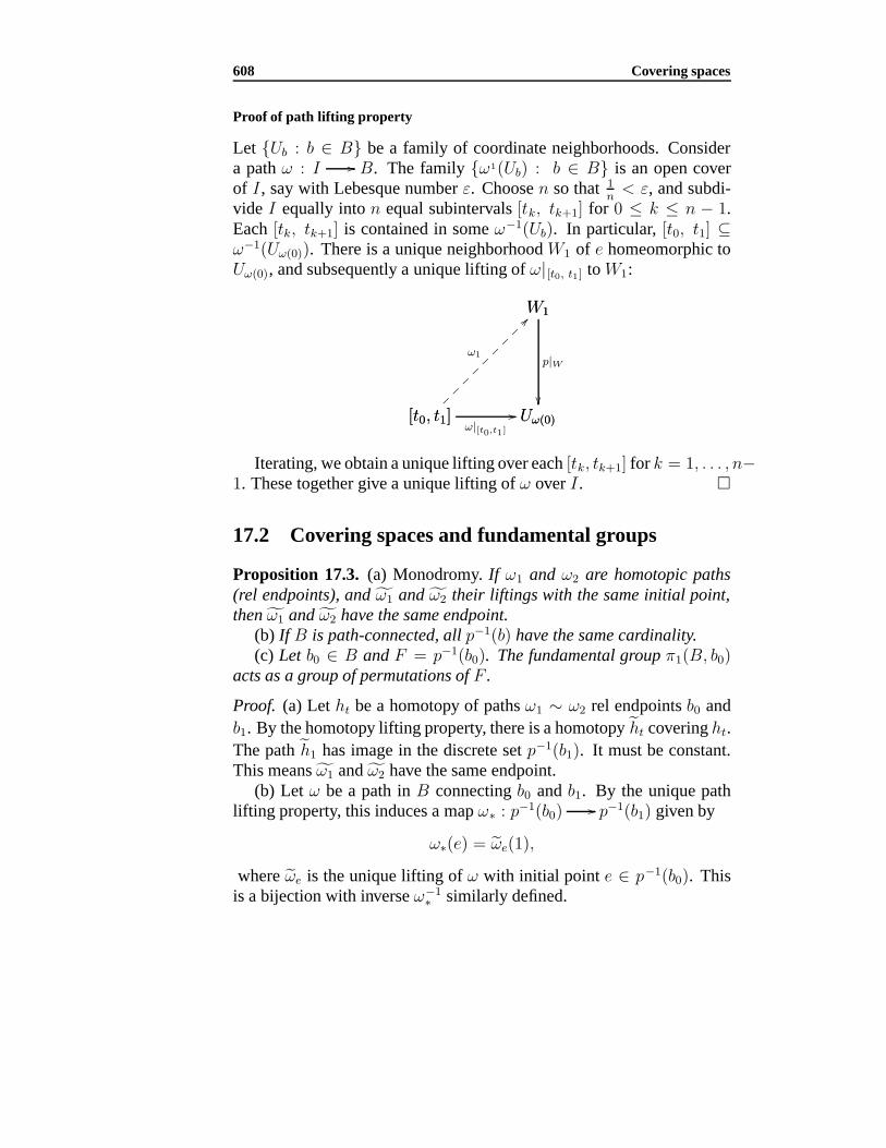
608 Covering spaces
Proof of path lifting property
Let Ub : b ∈ B be a family of coordinate neighborhoods. Considera path ω : I B. The family ω1(Ub) : b ∈ B is an open coverof I , say with Lebesque number ε. Choose n so that 1
n< ε, and subdi-
vide I equally into n equal subintervals [tk, tk+1] for 0 ≤ k ≤ n − 1.Each [tk, tk+1] is contained in some ω−1(Ub). In particular, [t0, t1] ⊆ω−1(Uω(0)). There is a unique neighborhood W1 of e homeomorphic toUω(0), and subsequently a unique lifting of ω|[t0, t1] to W1:
[t0, t1] Uω(0)ω|[t0,t1]
W1
[t0, t1]
ω1
W1
Uω(0)
p|W
Iterating, we obtain a unique lifting over each [tk, tk+1] for k = 1, . . . , n−1. These together give a unique lifting of ω over I .
17.2 Covering spaces and fundamental groups
Proposition 17.3. (a) Monodromy. If ω1 and ω2 are homotopic paths(rel endpoints), and ω1 and ω2 their liftings with the same initial point,then ω1 and ω2 have the same endpoint.
(b) If B is path-connected, all p−1(b) have the same cardinality.(c) Let b0 ∈ B and F = p−1(b0). The fundamental group π1(B, b0)
acts as a group of permutations of F .
Proof. (a) Let ht be a homotopy of paths ω1 ∼ ω2 rel endpoints b0 andb1. By the homotopy lifting property, there is a homotopy ht covering ht.The path h1 has image in the discrete set p−1(b1). It must be constant.This means ω1 and ω2 have the same endpoint.
(b) Let ω be a path in B connecting b0 and b1. By the unique pathlifting property, this induces a map ω∗ : p−1(b0) p−1(b1) given by
ω∗(e) = ωe(1),
where ωe is the unique lifting of ω with initial point e ∈ p−1(b0). Thisis a bijection with inverse ω−1
∗ similarly defined.
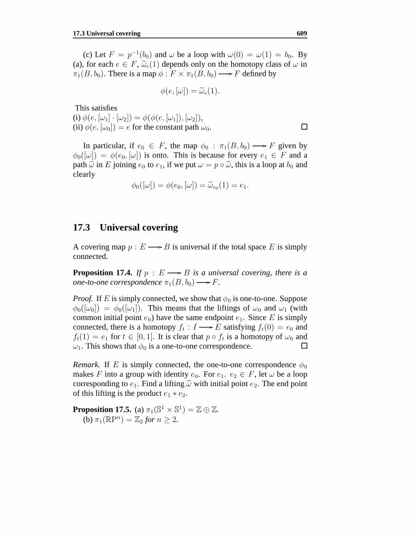
17.3 Universal covering 609
(c) Let F = p−1(b0) and ω be a loop with ω(0) = ω(1) = b0. By(a), for each e ∈ F , ωe(1) depends only on the homotopy class of ω inπ1(B, b0). There is a map φ : F × π1(B, b0) F defined by
φ(e, [ω]) = ωe(1).
This satisfies(i) φ(e, [ω1] · [ω2]) = φ(φ(e, [ω1]), [ω2]),(ii) φ(e, [ω0]) = e for the constant path ω0.
In particular, if e0 ∈ F , the map φ0 : π1(B, b0) F given byφ0([ω]) = φ(e0, [ω]) is onto. This is because for every e1 ∈ F and apath ω in E joining e0 to e1, if we put ω = p ω, this is a loop at b0 andclearly
φ0([ω]) = φ(e0, [ω]) = ωe0(1) = e1.
17.3 Universal covering
A covering map p : E B is universal if the total space E is simplyconnected.
Proposition 17.4. If p : E B is a universal covering, there is aone-to-one correspondence π1(B, b0) F .
Proof. If E is simply connected, we show that φ0 is one-to-one. Supposeφ0([ω0]) = φ0([ω1]). This means that the liftings of ω0 and ω1 (withcommon initial point e0) have the same endpoint e1. Since E is simplyconnected, there is a homotopy ft : I E satisfying ft(0) = e0 andft(1) = e1 for t ∈ [0, 1]. It is clear that p ft is a homotopy of ω0 andω1. This shows that φ0 is a one-to-one correspondence.
Remark. If E is simply connected, the one-to-one correspondence φ0
makes F into a group with identity e0. For e1, e2 ∈ F , let ω be a loopcorresponding to e1. Find a lifting ω with initial point e2. The end pointof this lifting is the product e1 ∗ e2.
Proposition 17.5. (a) π1(S1 × S1) = Z ⊕ Z.
(b) π1(RPn) = Z2 for n ≥ 2.
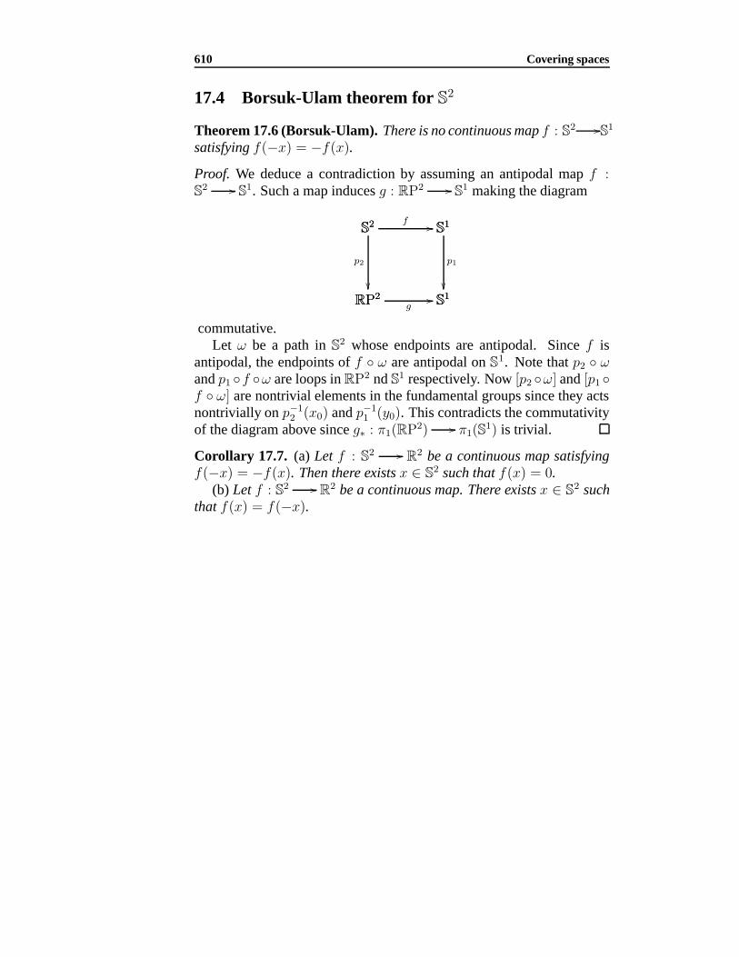
610 Covering spaces
17.4 Borsuk-Ulam theorem for S2
Theorem 17.6 (Borsuk-Ulam). There is no continuous map f : S2 S1
satisfying f(−x) = −f(x).
Proof. We deduce a contradiction by assuming an antipodal map f :S
2 S1. Such a map induces g : RP2 S1 making the diagram
RP2S
1g
S2
RP2
p2
S2 S1f S1
S1
p1
commutative.Let ω be a path in S2 whose endpoints are antipodal. Since f is
antipodal, the endpoints of f ω are antipodal on S1. Note that p2 ω
and p1 f ω are loops in RP2 nd S1 respectively. Now [p2 ω] and [p1 f ω] are nontrivial elements in the fundamental groups since they actsnontrivially on p−1
2 (x0) and p−11 (y0). This contradicts the commutativity
of the diagram above since g∗ : π1(RP2) π1(S1) is trivial.
Corollary 17.7. (a) Let f : S2 R2 be a continuous map satisfyingf(−x) = −f(x). Then there exists x ∈ S2 such that f(x) = 0.
(b) Let f : S2 R2 be a continuous map. There exists x ∈ S2 suchthat f(x) = f(−x).
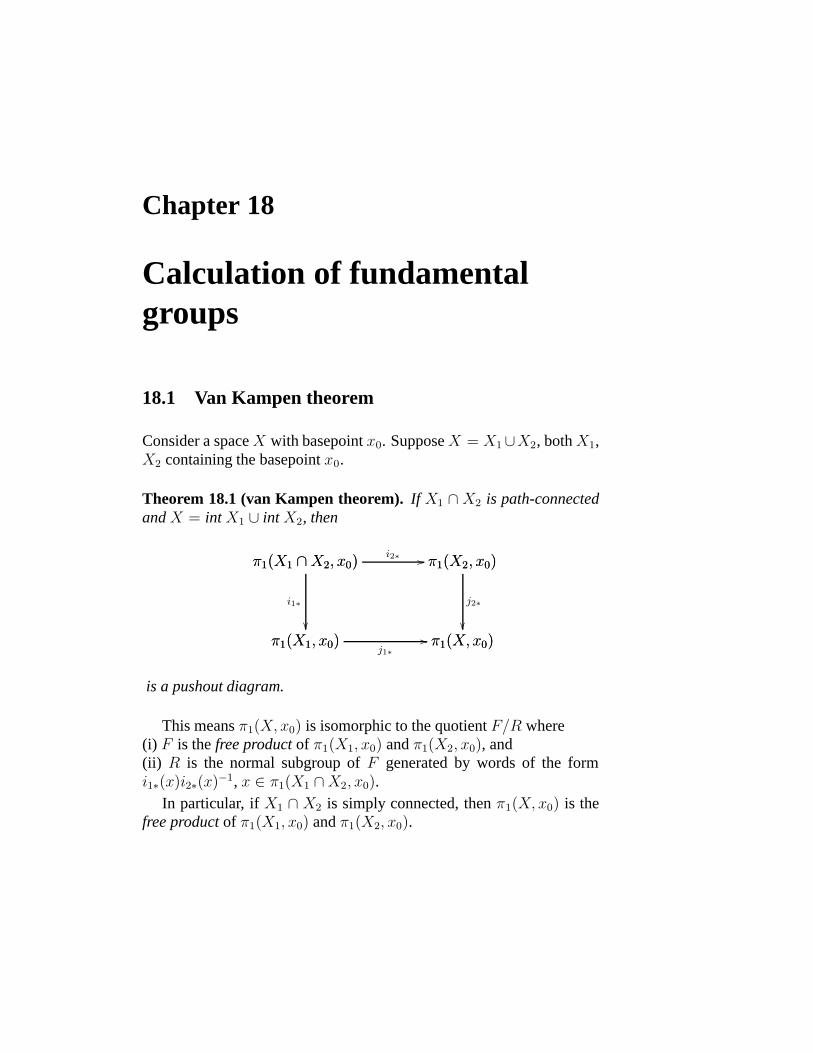
Chapter 18
Calculation of fundamentalgroups
18.1 Van Kampen theorem
Consider a space X with basepoint x0. Suppose X = X1∪X2, both X1,X2 containing the basepoint x0.
Theorem 18.1 (van Kampen theorem). If X1 ∩ X2 is path-connectedand X = int X1 ∪ int X2, then
π1(X1, x0) π1(X, x0)j1∗
π1(X1 ∩X2, x0)
π1(X1, x0)
i1∗
π1(X1 ∩X2, x0) π1(X2, x0)i2∗ π1(X2, x0)
π1(X, x0)
j2∗
is a pushout diagram.
This means π1(X, x0) is isomorphic to the quotient F/R where(i) F is the free product of π1(X1, x0) and π1(X2, x0), and(ii) R is the normal subgroup of F generated by words of the formi1∗(x)i2∗(x)−1, x ∈ π1(X1 ∩X2, x0).
In particular, if X1 ∩ X2 is simply connected, then π1(X, x0) is thefree product of π1(X1, x0) and π1(X2, x0).

612 Calculation of fundamental groups
Examples
(1) Consider the one-point union of two circles, S1∨S1. The fundamentalgroup π1(S
1 ∨ S1) is the free group on 2 generators.
≈
(2) π1(Sn) = 0 for n ≥ 2.
18.2 Fundamental group from triangulations
Chapter 19
Group structures on [X,Y ]
Let X and Y be given spaces with basepoints x0 and y0. We shall writesimply [X, Y ] for the set of homotopy classes of basepoint preservingmaps f : (X, x0) (Y, y0). We consider the possibility of endowingwith [X, Y ] a natural group structure.
19.1 Topological groups
A topological group is a group with a topology in which the multiplica-tion and inversion maps are continuous. Examples abound.
1. The real line R.2. The spheres S
n for n = 1, 3. S7 is not a topological group; it is an
H-space.3. The general linear groups GL(n).4. The orthogonal groups O(n) and special groups SO(n).If Y is a topological group, then for every X , the function space Y X
is a topological group: (f · g)(x) = f(x) · g(x) for x ∈ X . This inducesa group operation on [X, Y ]:
[f ] · [g] = [f · g].
19.2 H-spaces
Let (Y, y0) be a space with basepoint. Denote by d : Y Y × Y thediagonal map d(x) = (x, x). We say that Y is an H-space if there are
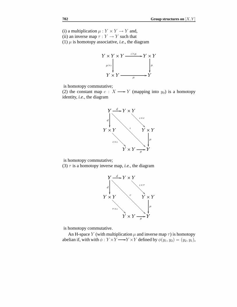
702 Group structures on [X, Y ]
(i) a multiplication µ : Y × Y → Y and,(ii) an inverse map τ : Y → Y such that(1) µ is homotopy associative, i.e., the diagram
Y × Y Yµ
Y × Y × Y
Y × Y
µ×ι
Y × Y × Y Y × Yι×µ Y × Y
Y
µ
is homotopy commutative;(2) the constant map c : X Y (mapping into y0) is a homotopyidentity, i.e., the diagram
Y Y × Yd Y
Y × Y
d
Y × Y
Y × Y
ι×c
Y × Y
Y
µ
Y
Y
ι
Y × Y
Y × Y
c×ι
Y × Y Yµ
is homotopy commutative;(3) τ is a homotopy inverse map, i.e., the diagram
Y Y × Yd Y
Y × Y
d
Y × Y
Y × Y
ι×τ
Y × Y
Y
µ
Y
Y
c
Y × Y
Y × Y
τ×ι
Y × Y Yµ
is homotopy commutative.An H-space Y (with multiplication µ and inverse map τ ) is homotopy
abelian if, with with φ : Y ×Y Y ×Y defined by φ(y1, y2) = (y2, y1),

19.2 H-spaces 703
the diagram
Y × Y
Y
µ
Y × Y Y × Yφ Y × Y
Y
µ
is homotopy commutative. If Y is homotopy abelian, then the group[X, Y ] is abelian.
Let (Y1, µ1) and (Y2, µ2) be H-spaces. A map f : Y1 Y2 is called
an H-map if the diagram
Y1 Y2f
Y1 × Y1
Y1
µ1
Y1 × Y1 Y2 × Y2f×f Y2 × Y2
Y2
µ2
is homotopy commutative.
Proposition 19.1. Let Y be a space with basepoint y0. Then [−, Y ] is afunctor into the category of groups if and only if Y is an H-space.
Proof. It is enough to prove the necessity part. Assume that the functor[−, Y ] : Top Set lifts into Grp, i.e., there is a natural groupstructure on each [X, Y ]. We show this assumption uniquely determinesan H-space structure on Y . Let p1, p2 : Y × Y Y be the projectionsfrom the first and second factors respectively. Choose(i) µ : Y × Y Y such that
[µ] = [p1] + [p2]
in [Y × Y, Y ], 1
(ii) τ : Y Y such that [τ ] = −[ιY ].We show that for any space X with basepoint x0, the group structure
on [X, Y ] is determined by µ:
[µ(u× v)] =(u× v)∗([p1] + [p2])
=(u× v)∗([p1]) + (u× v)∗([p2])
=[u] + [v].
1Note that the choice of [µ] giving rise to a fixed operation is unique since [p1]+ [p2] = [µ(p1 ×p2)] =[µ].
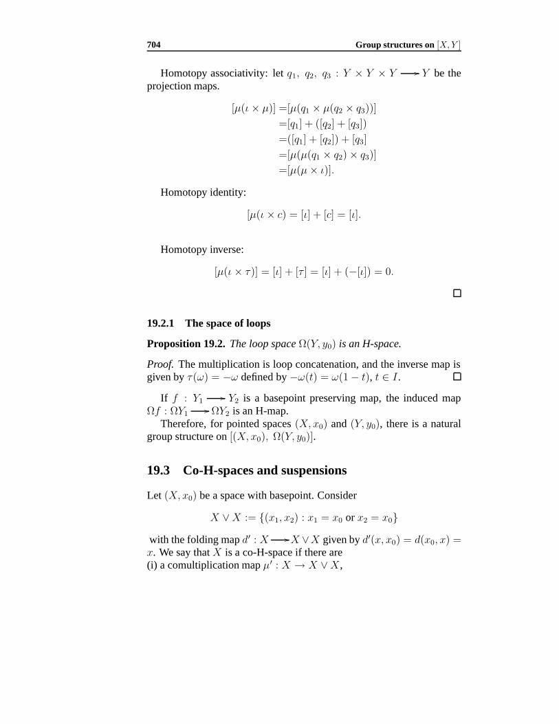
704 Group structures on [X, Y ]
Homotopy associativity: let q1, q2, q3 : Y × Y × Y Y be theprojection maps.
[µ(ι× µ)] =[µ(q1 × µ(q2 × q3))]
=[q1] + ([q2] + [q3])
=([q1] + [q2]) + [q3]
=[µ(µ(q1 × q2)× q3)]
=[µ(µ× ι)].
Homotopy identity:
[µ(ι× c) = [ι] + [c] = [ι].
Homotopy inverse:
[µ(ι× τ)] = [ι] + [τ ] = [ι] + (−[ι]) = 0.
19.2.1 The space of loops
Proposition 19.2. The loop space Ω(Y, y0) is an H-space.
Proof. The multiplication is loop concatenation, and the inverse map isgiven by τ(ω) = −ω defined by −ω(t) = ω(1− t), t ∈ I .
If f : Y1 Y2 is a basepoint preserving map, the induced map
Ωf : ΩY1 ΩY2 is an H-map.
Therefore, for pointed spaces (X, x0) and (Y, y0), there is a naturalgroup structure on [(X, x0), Ω(Y, y0)].
19.3 Co-H-spaces and suspensions
Let (X, x0) be a space with basepoint. Consider
X ∨X := (x1, x2) : x1 = x0 or x2 = x0with the folding map d′ : X X ∨X given by d′(x, x0) = d(x0, x) =x. We say that X is a co-H-space if there are(i) a comultiplication map µ′ : X → X ∨X ,
19.3 Co-H-spaces and suspensions 705
(ii) an inverse map τ ′ : X X such that(1) µ′ is homotopy associative, i.e., the diagram
X ∨X X ∨X ∨Xι∨µ′
X
X ∨X
µ′
X X ∨Xµ′
X ∨X
X ∨X ∨X
µ′∨ι
is homotopy associative;(2) the constant map c : X X is a homotopy identity, i.e., the diagram
X X ∨Xµ′
X
X ∨X
µ′
X ∨X
X ∨X
ι∨c
X ∨X
X
d′
X
X
ι
X ∨X
X ∨X
c∨ι
X ∨X Xd′
is homotopy commutative;(iii) τ ′ is a homotopy inverse, i.e., the diagram
X X ∨Xµ′
X
X ∨X
µ′
X ∨X
X ∨X
ι∨τ ′
X ∨X
X
d′
X
X
c
X ∨X
X ∨X
τ ′∨ι
X ∨X Xd′
is homotopy commutative.
19.3.1 The reduced suspension
Let (X, x0) be a pointed space. The reduced suspension of X is thespace
ΣX := X × I/(X × 0, 1 ∪ x0 × I).
706 Group structures on [X, Y ]
It has basepoint [x0, t] = [x, 0] = [x, 1], t ∈ [0, 1]. ΣX has a naturalcomultiplication
µ′([x, t]) =
[x, 2t], ∗, 0 ≤ t ≤ 1
2,
∗, [x, 2t− 1], 12≤ t ≤ 1.
τ ′[x, t] =[x, 1− t].
This makes ΣX into a co-H-space.
Proposition 19.3. For every space Y , there is a natural group structureon [ΣX, Y ].
Proposition 19.4. [ΣX, Y ] and [X, ΩY ] are naturally isomorphic.
Proof. There is a homeomorphism Θ : Y ΣX (ΩY )X given by
Θ(f)(x)(t) = f [x, t].
This induces an isomorphism [ΣX, Y ] [X, ΩY ].
Proposition 19.5. If X is co-H-space and Y an H-space, then the groupstructures induced on [X, Y ] are the same, and are abelian.
Proof. Denote by + the group operation on [X, Y ] induced by the H-space structure of Y , and by +′ that induced by the co-H-space structureof X . Let p, q, r, s : X Y be arbitrary maps.
([p] + [q]) +′ ([r] + [s]) =d′(µ(p× q)d ∨ µ(r × s)d)µ′,=d′(µ ∨ µ)((p× q) ∨ (r × s)(d ∨ d)µ′;
([p] +′ [r]) + ([q] +′ [s]) =µ(d′(p ∨ r)µ′ × d′(q ∨ s)µ′)d,=µ(d′ × d′)((p ∨ r)× (q ∨ s))(µ′ ∨ µ′)d.
The result
([p] + [q]) +′ ([r] + [s]) = ([p] +′ [r]) + ([q] +′ [s])
follows from the homotopy commutativity of the diagram
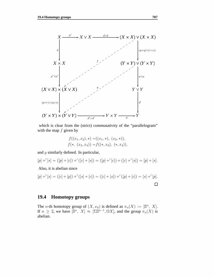
19.4 Homotopy groups 707
X X ∨Xµ′
X ∨X (X ×X) ∨ (X ×X)d∨d X
X ×X
d
X ×X
(X ∨X)× (X ∨X)
µ′∨µ′
(X ∨X)× (X ∨X)
(Y × Y )× (Y ∨ Y )
(p∨r)×(q∨s)
(Y × Y )× (Y ∨ Y ) Y × Y
d′×d′ Y × Y Yµ
(X ×X) ∨ (X ×X)
(Y × Y ) ∨ (Y × Y )
(p×q)∨(r×s)
(Y × Y ) ∨ (Y × Y )
Y ∨ Y
µ∨µ
Y ∨ Y
Y
d′
(X ×X) ∨ (X ×X)
(X ∨X)× (X ∨X)
f
(Y × Y ) ∨ (Y × Y )
(Y × Y )× (Y ∨ Y )
g
which is clear from the (strict) commutativity of the “parallelogram”with the map f given by
f((x1, x2), ∗) =((x1, ∗), (x2, ∗)),f(∗, (x3, x4)) =f((∗, x3), (∗, x4)),
and g similarly defined. In particular,
[p]+′ [s] = ([p]+ [c])+′ ([c]+ [s]) = ([p]+′ [c])+ ([c]+′ [s]) = [p]+ [s].
Also, it is abelian since
[p]+′ [s] = ([c]+ [p])+′ ([s]+ [c]) = ([c]+ [s])+′ ([p]+ [c]) = [s]+′ [p].
19.4 Homotopy groups
The n-th homotopy group of (X, x0) is defined as πn(X) := [Sn, X].If n ≥ 2, we have [Sn, X] ≈ [ΣSn−1,ΩX], and the group πn(X) isabelian.
708 Group structures on [X, Y ]
Examples
(1) If X is contractible, then πn(X) = 0 for every n ≥ 1.(2) If m < n, then πm(S
n) = 0.
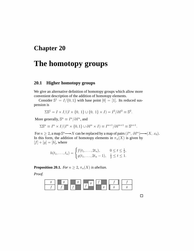
Chapter 20
The homotopy groups
20.1 Higher homotopy groups
We give an alternative definition of homotopy groups which allow moreconvenient description of the addition of homotopy elements.
Consider S1 = I/0, 1 with base point [0] = [1]. Its reduced sus-pension is
ΣS1 = I × I/(I × 0, 1 ∪ 0, 1 × I) = I2/∂I2 ≡ S
2.
More generally, Sn ≡ In/∂In, and
ΣSn ≡ In × I/(In × 0, 1 ∪ ∂In × I) ≡ In+1/∂In+1 ≡ S
n+1.
For n ≥ 2, a map Sn X can be replaced by a map of pairs (In, ∂In) (X, x0).In this form, the addition of homotopy elements in πn(X) is given by[f ] + [g] = [h], where
h(t1, . . . , tn) =
f(t1, . . . , 2tn), 0 ≤ t ≤ 1
2,
g(t1, . . . , 2tn − 1), 12≤ t ≤ 1.
Proposition 20.1. For n ≥ 2, πn(X) is abelian.
Proof.
f
g
f
g
f
g
fg f
g
f
g
f
g
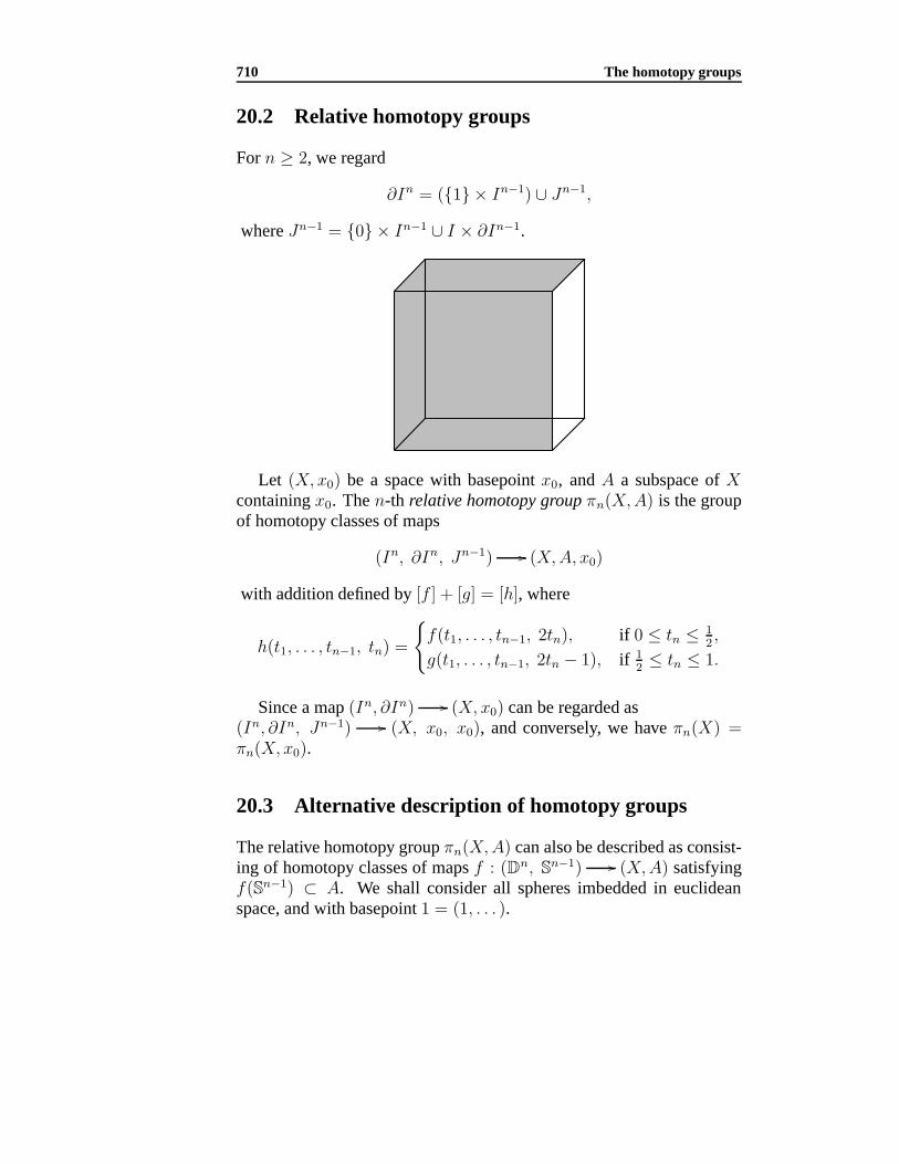
710 The homotopy groups
20.2 Relative homotopy groups
For n ≥ 2, we regard
∂In = (1 × In−1) ∪ Jn−1,
where Jn−1 = 0 × In−1 ∪ I × ∂In−1.
Let (X, x0) be a space with basepoint x0, and A a subspace of Xcontaining x0. The n-th relative homotopy group πn(X,A) is the groupof homotopy classes of maps
(In, ∂In, Jn−1) (X,A, x0)
with addition defined by [f ] + [g] = [h], where
h(t1, . . . , tn−1, tn) =
f(t1, . . . , tn−1, 2tn), if 0 ≤ tn ≤ 1
2,
g(t1, . . . , tn−1, 2tn − 1), if 12≤ tn ≤ 1.
Since a map (In, ∂In) (X, x0) can be regarded as(In, ∂In, Jn−1) (X, x0, x0), and conversely, we have πn(X) =πn(X, x0).
20.3 Alternative description of homotopy groups
The relative homotopy group πn(X,A) can also be described as consist-ing of homotopy classes of maps f : (Dn, Sn−1) (X,A) satisfyingf(Sn−1) ⊂ A. We shall consider all spheres imbedded in euclideanspace, and with basepoint 1 = (1, . . . ).
20.4 The homotopy exact sequence of a pair 711
The sum of homotopy elements can be determined as follows. Let En+
and En− be the northern and southern hemispheres respectively. There are
homotopies ι ∼ θ± : Dn Dn such that
θ+(x1, . . . , xn) =1, if xn ≤ 0;
θ−(x1, . . . , xn) =1, if xn ≥ 0.
Then for f, g : (Dn, Sn−1) (X,A), the homotopy class [f ] + [g]is represented by h : (Dn, Sn−1) (X,A), where
h(x1, . . . , xn) =
f θ+(x1, . . . , xn), if xn ≤ 0;
f θ−(x1, . . . , xn), if xn ≥ 0.
Lemma 20.2. A map f : Sn X is nullhomotopic if and only if it canbe extended to g : Dn+1 X .
Lemma 20.3. A map f : (Dn, Sn−1) (X,A) represents the zeroelement in πn(X,A) if and only if there is a homotopy ft : Dn Xsuch that f0 = f and f1(D
n) ⊂ A.
Proof. (⇐) It is enough to assume f(Dn) ⊂ A. Since Dn is contractible,there is a homotopy gt : Dn A with g0 = f and g1 = c constant map.This can be regarded as a homotopy gt : (D
n, Sn−1) (X,A).(⇒) We begin with a homotopy f ∼ c : (Dn, Sn−1) (X,A) as a
map defined on the cone with base Dn × 0 and vertex (0, 1) ∈ R
n × I .We may assume that the “surface” of the cone is mapping into A. Thismap can be extended to the cyclinder Dn × I by “laying radii alonggenerators” to give a homotopy satisfying the requirement.
20.4 The homotopy exact sequence of a pair
Given a pair (X,A), we consider the inclusion mapsi : A X and j : (X, x0) (X, A). These induce, for each n ≥ 0,homomorphismsi∗ : πn(A) πn(X) and j∗ : πn(X) πn(X,A).
There is also a family of boundary homomorphisms∂n : πn(X,A) πn−1(A) defined geometrically by
∂n([f ]) := [f |1×In−1] for every f : (In, ∂In, Jn−1) (X,A, x0),
712 The homotopy groups
or∂n([f ]) = [f |Sn−1]
if f is represented by (Dn, Sn−1) (X,A).
Theorem 20.4. In the sequence
· · · πn(A)i∗ πn(X)
j∗ πn(X,A)∂n πn−1(A)
i∗ πn−1(X) · · · ,(1) ker j∗ = Im i∗,
(2) ker ∂n = Im j∗,(3) ker i∗ = Im ∂n.
This is summarized by saying the sequence above is exact. We callthis the homotopy exact sequence of the pair (X,A).
Proof. (1a) First note that j∗ i∗ = 0 by Lemma 20.3 since for everyf : (Dn, Sn−1) (A, x0), j∗i∗[f ] = [j i f ] is represented by a map
(Dn, Sn−1) (A, x0) (X, x0) (X,A)
whose image is in A. Therefore, Im j∗ ⊂ ker i∗.(1b) Suppose f : (Dn, Sn−1) (X, x0) satisfies j∗([f ]) = 0 ∈
πn(X,A). There is a homotopy gt : (Dn, Sn−1) (X,A) with
(i) g1(Dn) ⊂ A,
(ii) gt|Sn−1 = j f |Sn−1 for every t ∈ I , i.e., gt(Dn) = x0. Therefore,there is a factorization
g1 : (Dn, Sn−1)
g (A, x0)i (X, x0)
j (X,A).
Now, g1 ∼ j f ⇒ i g ∼ f ⇒ i∗([g]) = [f ]. This means thatker j∗ ⊂ Im i∗.
(2a) For any g : (Dn, Sn−1) (X, x0), clearly j g|Sn−1 is theconstant map. This means ∂n(j∗([g])) = 0 and Im j∗ ⊂ ker ∂n.
(2b) Suppose f : (Dn, Sn−1) (X,A) satisfies [f |Sn−1 ] = 0. Thereis a map H : Dn × 0 ∪ Sn−1 × I X for which H(Sn−1 × 1) = x0.This can be extended to a map H : D
n × I X with
H1 : (Dn, Sn−1)
h (X, x0)j (X,A).
Clearly, [f ] = [H1] = j∗([h]). This shows that ker ∂n ⊂ Im j∗.
20.5 Appendix: calculations with exact sequences 713
(3a) Consider f : (Dn, Sn−1) (A,A). The homotopy classi∗∂n([f ]) is represented by the composite
(Sn−1, 1)f |
Sn−1 (A, x0)( X, x0).
This is nullhomotopic since it can be extended to Dn. This shows thatIm ∂n ⊂ ker i∗.
(3b) Let g : Sn−1 A be a map with i g : Sn−1 A Xnullhomotopic. Extend this to f : D
X , which can be regarded as a
map f : (Dn, Sn−1) (X,A). Clearly, ∂n([f ]) = [g]. This shows thatker i∗ ⊂ Im ∂n.
Example 20.1. πm(Dn, Sn−1).
Since Dn+1 is contractible and πm(D
n+1) = 0 for every m ≥ 0,from the homotopy exact sequence of the pair (Dn+1, Sn), we have anisomorphism : πm(D
n+1, Sn) ≈ πm−1(S
n).
20.5 Appendix: calculations with exact sequences
A sequence of (abelian) groups and homomorphisms
(E) : · · · αn+2
An+1 αn+1
An αn An−1 αn−1
An−2 · · ·
is exact if for every n, Im αn+1 = kerαn.
Proposition 20.5. In the exact sequence (E), the following are equiva-lent.(i) αn+1 is an epimorphism.(ii) αn = 0.(iii) αn−1 is a monomorphism.
Proposition 20.6. Consider a short exact sequence
0 Af B
g C 0.
The following statements are equivalent.(i) B ≈ A⊕ C.(ii) g has a right inverse.(iii) f has a left inverse.
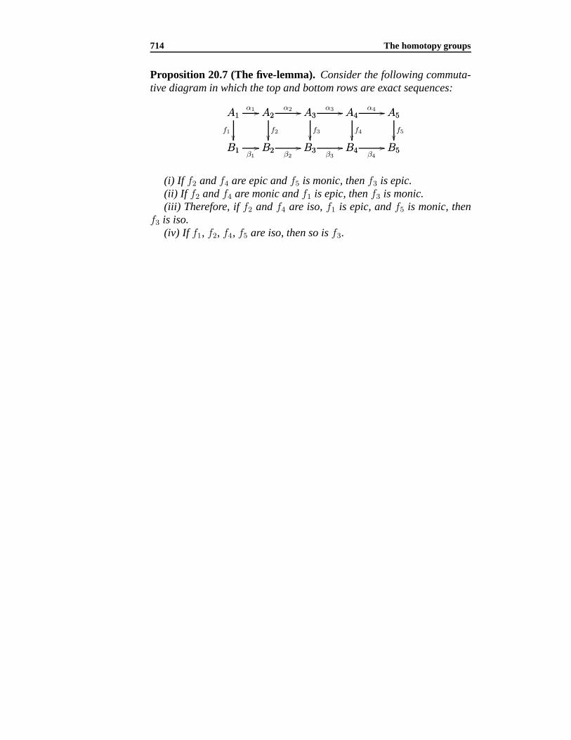
714 The homotopy groups
Proposition 20.7 (The five-lemma). Consider the following commuta-tive diagram in which the top and bottom rows are exact sequences:
B1 B2β1
A1
B1
f1
A1 A2α1 A2
B2
f2
B3β2
A3α2 A3
B3
f3
B4β3
A4α3 A4
B4
f4
B5β4
A5α4 A5
B5
f5
(i) If f2 and f4 are epic and f5 is monic, then f3 is epic.(ii) If f2 and f4 are monic and f1 is epic, then f3 is monic.(iii) Therefore, if f2 and f4 are iso, f1 is epic, and f5 is monic, then
f3 is iso.(iv) If f1, f2, f4, f5 are iso, then so is f3.
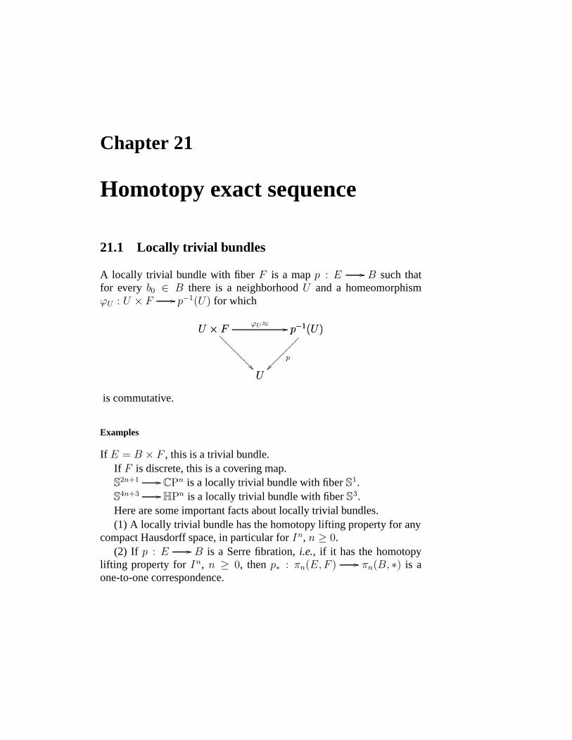
Chapter 21
Homotopy exact sequence
21.1 Locally trivial bundles
A locally trivial bundle with fiber F is a map p : E B such thatfor every b0 ∈ B there is a neighborhood U and a homeomorphismϕU : U × F p−1(U) for which
U × F
U
U × F p−1(U)
ϕU≈ p−1(U)
U
p
is commutative.
Examples
If E = B × F , this is a trivial bundle.If F is discrete, this is a covering map.S2n+1 CPn is a locally trivial bundle with fiber S1.S4n+3 HPn is a locally trivial bundle with fiber S3.Here are some important facts about locally trivial bundles.(1) A locally trivial bundle has the homotopy lifting property for any
compact Hausdorff space, in particular for In, n ≥ 0.(2) If p : E B is a Serre fibration, i.e., if it has the homotopy
lifting property for In, n ≥ 0, then p∗ : πn(E,F ) πn(B, ∗) is aone-to-one correspondence.
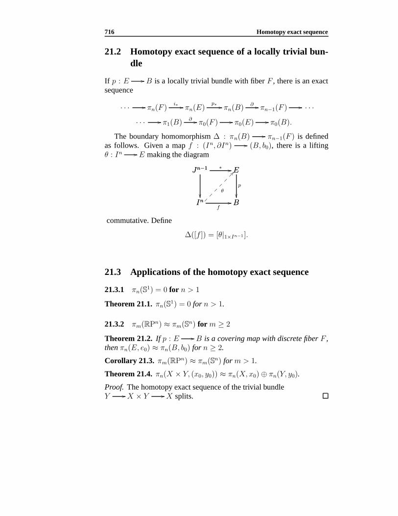
716 Homotopy exact sequence
21.2 Homotopy exact sequence of a locally trivial bun-dle
If p : E B is a locally trivial bundle with fiber F , there is an exactsequence
· · · πn(F )i∗ πn(E)
p∗ πn(B)∂ πn−1(F ) · · ·
· · · π1(B)∂ π0(F ) π0(E) π0(B).
The boundary homomorphism ∆ : πn(B) πn−1(F ) is definedas follows. Given a map f : (In, ∂In) (B, b0), there is a liftingθ : In E making the diagram
In Bf
Jn−1
In
Jn−1 E∗ E
B
p
θ
commutative. Define
∆([f ]) = [θ|1×In−1 ].
21.3 Applications of the homotopy exact sequence
21.3.1 πn(S1) = 0 for n > 1
Theorem 21.1. πn(S1) = 0 for n > 1.
21.3.2 πm(RPn) ≈ πm(Sn) for m ≥ 2
Theorem 21.2. If p : E B is a covering map with discrete fiber F ,then πn(E, e0) ≈ πn(B, b0) for n ≥ 2.
Corollary 21.3. πm(RPn) ≈ πm(Sn) for m > 1.
Theorem 21.4. πn(X × Y, (x0, y0)) ≈ πn(X, x0)⊕ πn(Y, y0).
Proof. The homotopy exact sequence of the trivial bundleY X × Y X splits.
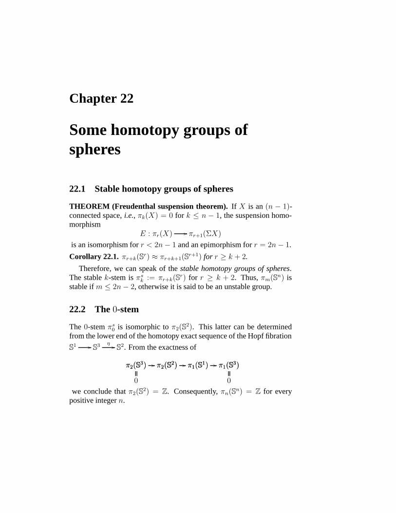
Chapter 22
Some homotopy groups ofspheres
22.1 Stable homotopy groups of spheres
THEOREM (Freudenthal suspension theorem). If X is an (n − 1)-connected space, i.e., πk(X) = 0 for k ≤ n − 1, the suspension homo-morphism
E : πr(X) πr+1(ΣX)
is an isomorphism for r < 2n− 1 and an epimorphism for r = 2n− 1.
Corollary 22.1. πr+k(Sr) ≈ πr+k+1(S
r+1) for r ≥ k + 2.
Therefore, we can speak of the stable homotopy groups of spheres.The stable k-stem is πs
k := πr+k(Sr) for r ≥ k + 2. Thus, πm(S
n) isstable if m ≤ 2n− 2, otherwise it is said to be an unstable group.
22.2 The 0-stem
The 0-stem πs0 is isomorphic to π2(S
2). This latter can be determinedfrom the lower end of the homotopy exact sequence of the Hopf fibration
S1 S3 η S2. From the exactness of
π2(S3) π2(S
2) π2(S2) π1(S
1) π1(S1) π1(S
3)π2(S3)
0
π1(S3)
0
we conclude that π2(S2) = Z. Consequently, πn(S
n) = Z for everypositive integer n.
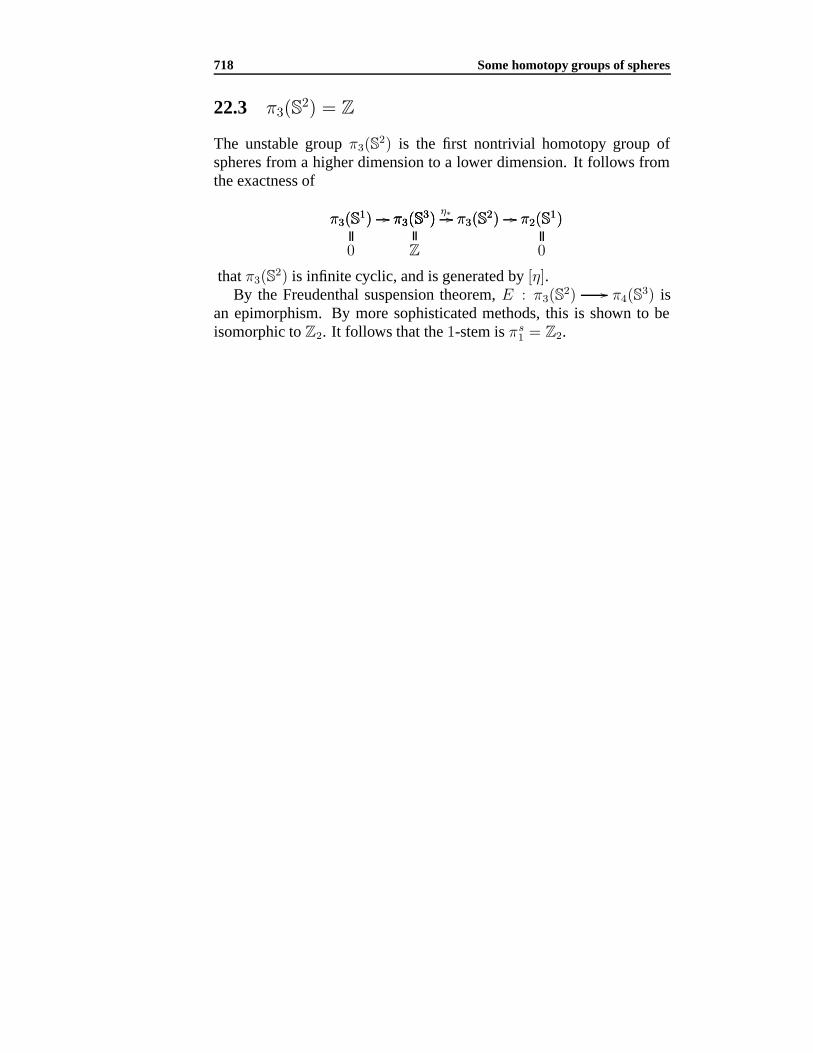
718 Some homotopy groups of spheres
22.3 π3(S2) = Z
The unstable group π3(S2) is the first nontrivial homotopy group of
spheres from a higher dimension to a lower dimension. It follows fromthe exactness of
π3(S1) π3(S
3) π3(S3) π3(S
2)η∗ π3(S
2) π2(S1)π3(S
1)
0
π2(S1)
0
π3(S3)
Z
that π3(S2) is infinite cyclic, and is generated by [η].
By the Freudenthal suspension theorem, E : π3(S2) π4(S
3) isan epimorphism. By more sophisticated methods, this is shown to beisomorphic to Z2. It follows that the 1-stem is πs
1 = Z2.
Chapter 23
Smooth manifolds
23.1 Smooth maps
Let X ⊂ Rk, Y ⊂ Rn and f : X Y be a continuous map.(1) If X is open in R
k, we say that f is smooth if all partial derivativesexist and are continuous.
(2) More generally, if X is not necessarily open in Rk, we say that f
is smooth at x ∈ X if it is the restriction of a smooth map on an openset Wx ⊂ Rk, i.e., there exists an open set Wx ⊂ Rk and a smooth mapF : Wx
Rn that F |W∩X = f |Wx∩X . Finally, f is smooth if it issmooth at each x ∈ X .
f : X Y is called a diffeomorphism if(i) it is a homeomorphism,(ii) both f and f−1 are smooth maps.
X ⊂ Rk and Y ⊂ R
n are diffeomorphic if there is a diffeomorphismbetween them.
Diffeomorphism is an equivalence relation.
23.2 Smooth manifolds
M ⊂ Rk is called a smooth manifold of dimension m if each pointx ∈ M has a neighborhood diffeomorphic to an open subset of Rm, i.e.,for each x ∈ M , there are(i) an open set Wx ⊂ Rk with x ∈ Wx ∩M ,(ii) an open set U ⊂ Rm, and(iii) a diffeomorphism ϕx : U Wx∩M called a local parametrizationat x ∈ M .
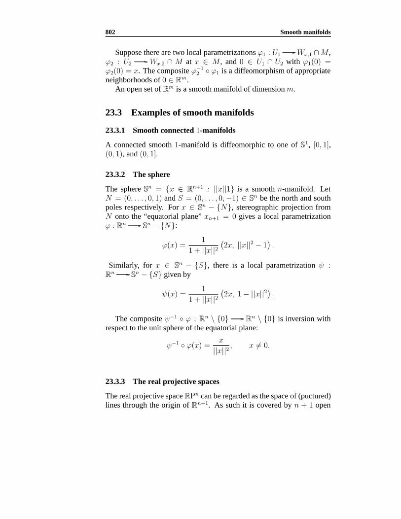
802 Smooth manifolds
Suppose there are two local parametrizations ϕ1 : U1 Wx,1 ∩M ,
ϕ2 : U2 Wx,2 ∩ M at x ∈ M , and 0 ∈ U1 ∩ U2 with ϕ1(0) =
ϕ2(0) = x. The composite ϕ−12 ϕ1 is a diffeomorphism of appropriate
neighborhoods of 0 ∈ Rm.An open set of Rm is a smooth manifold of dimension m.
23.3 Examples of smooth manifolds
23.3.1 Smooth connected 1-manifolds
A connected smooth 1-manifold is diffeomorphic to one of S1, [0, 1],(0, 1), and (0, 1].
23.3.2 The sphere
The sphere Sn = x ∈ Rn+1 : ||x||1 is a smooth n-manifold. LetN = (0, . . . , 0, 1) and S = (0, . . . , 0,−1) ∈ Sn be the north and southpoles respectively. For x ∈ Sn − N, stereographic projection fromN onto the “equatorial plane” xn+1 = 0 gives a local parametrizationϕ : Rn Sn − N:
ϕ(x) =1
1 + ||x||2(2x, ||x||2 − 1
).
Similarly, for x ∈ Sn − S, there is a local parametrization ψ :Rn Sn − S given by
ψ(x) =1
1 + ||x||2(2x, 1− ||x||2) .
The composite ψ−1 ϕ : Rn \ 0 Rn \ 0 is inversion withrespect to the unit sphere of the equatorial plane:
ψ−1 ϕ(x) =x
||x||2 , x = 0.
23.3.3 The real projective spaces
The real projective space RPn can be regarded as the space of (puctured)lines through the origin of Rn+1. As such it is covered by n + 1 open
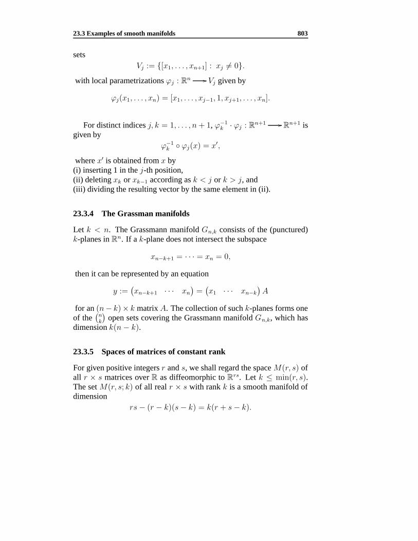
23.3 Examples of smooth manifolds 803
setsVj := [x1, . . . , xn+1] : xj = 0.
with local parametrizations ϕj : Rn Vj given by
ϕj(x1, . . . , xn) = [x1, . . . , xj−1, 1, xj+1, . . . , xn].
For distinct indices j, k = 1, . . . , n+ 1, ϕ−1k · ϕj : R
n+1 Rn+1 isgiven by
ϕ−1k ϕj(x) = x′,
where x′ is obtained from x by(i) inserting 1 in the j-th position,(ii) deleting xk or xk−1 according as k < j or k > j, and(iii) dividing the resulting vector by the same element in (ii).
23.3.4 The Grassman manifolds
Let k < n. The Grassmann manifold Gn,k consists of the (punctured)k-planes in Rn. If a k-plane does not intersect the subspace
xn−k+1 = · · · = xn = 0,
then it can be represented by an equation
y :=(xn−k+1 · · · xn
)=(x1 · · · xn−k
)A
for an (n− k)× k matrix A. The collection of such k-planes forms oneof the
(nk
)open sets covering the Grassmann manifold Gn,k, which has
dimension k(n− k).
23.3.5 Spaces of matrices of constant rank
For given positive integers r and s, we shall regard the space M(r, s) ofall r × s matrices over R as diffeomorphic to R
rs. Let k ≤ min(r, s).The set M(r, s; k) of all real r × s with rank k is a smooth manifold ofdimension
rs− (r − k)(s− k) = k(r + s− k).

804 Smooth manifolds
23.4 Appendix: Milnor’s proof of the fundamental the-orem of algebra
Consider the sphere S2 with stereographic projections ϕ and ψ from thenorth and south poles respectively. Let P : C C be a polynomial ofdegree n.
Conjugating P by ϕ, we obtain a smooth map f : S2 S2. Furtherconjugating f by ψ−1 we have a map g smooth in a neighborhood of 0.Indeed,
g(z) =zn
a0 + a1z + · · ·+ anzn.
Therefore, f is smooth in a neighborhood of the north pole.Now, f has a finite number of critical points. The set of regular values
of f is S2 with a finite number of points removed. It is connected. Since
#f−1(y) is locally constant for the regular values, it is actually constant.Since this number cannot be zero everywhere, it is zero nowhere. Thismeans that f is surjective and P must have a zero.
Chapter 24
Mappings between manifolds
24.1 Tangent space
Let M ⊂ Rk be a smooth manifold of dimension m. Consider x ∈ M .For every local parametrization ϕx : U Wx ∩ M ⊂ Rk, the imageof the differential dϕx : Rm Rk is independent of the choice of Uand ϕ, and is defined to be the tangent space of M at x, denoted τx(M).Note that dim τx(M) = m.
Let Mm ⊂ Rk and Nn ⊂ R2 be smooth manifolds, and f : M Na smooth map. For every x ∈ M , there is an induced map
dfx : τx(M) τf(x)(N)
called the differential of f at x, defined as follows. Choose an open setWx ∈ Rk and a smooth map F : Wx
R2 agreeing with f on Wx∩M ,and set dfx(u) = dFx(u) for every u ∈ τx(M).
(i) dfx(u) ∈ τf(x)(N) and is independent of the choice of Wx and F .(ii) dfx : τx(M) τf(x)(N) is a linear map.
Proposition 24.1 (The Chain rule). If f : M N and g : N Pare smooth maps between smooth manifolds, then for every x ∈ M ,
d(g f)x = dgf(x) dfx.
Theorem 24.2 (Inverse function theorem). Let f : M N a smoothmap. If dfx : τx(M) τf(x)(N) is an isomorphism, then f is a localdiffeomorphism.
Remark. Let ϕ : U M and ψ : V N be local parametrizations atx ∈ M and f(x) ∈ N respectively with ϕ(0) = x and ψ(0) = f(x). dfx
806 Mappings between manifolds
is an isomorphism if and only if the Jacobian of ψ f ψ−1 : U Vhas nonzero determinant at 0 ∈ U .
Theorem 24.3 (Inverse image theorem). Let f : M N be a smoothmap. If y ∈ N is a regular value in the sense that dfx : τx(M) τf(x)(N)is surjective for every x ∈ f−1(y) (assumed nonempty), then f−1(y) is asubmanifold of M , of dimension m− n.
24.2 Approximation of continuous map by a smooth one
1. Every compact manifold N can be given a Riemannian metric, i.e.,a positive definite inner product on each tangent space, which induces ametric ρ on N .
2. For compact manifolds M , N , the function space C(M,N) is ametric space:
ρ(f, g) = maxx∈M
ρ(f(x), g(x))
3. Let M , N be compact manifolds. Given a metric on N , there existsε > 0 such that two continuous maps f, g : M N are homotopicwhenever ρ(f, g) < ε.
4. Given a continuous map f : M N and ε > 0, there exists asmooth map g : M N such that ρ(f, g) < ε.
Theorem 24.4. (A) Every continuous map f : M N between com-pact, smooth manifolds is homotopic to some smooth map g : M N .
(B) If f, g : M N are homotopic smooth maps, they are smoothlyhomotopic.
24.3 Regular and critical values
24.3.1 Sets of measure zero
A cube in Rn is a product of intervals∏n
i=1[an, bn], and has volume(measure)
∏ni=1(bi − ai). A subset A ⊂ Rn has measure zero if it can be
covered by a countable collection of cubes having arbitrarily small totalvolume.
Let Mm be a smooth manifold of dimension m. A subset A ⊂ M hasmeasure zero if for any local parametrization ϕ : U M , ϕ−1(A) hasmeasure zero in Rm.
24.3 Regular and critical values 807
24.3.2 Sard’s theorem
Let f : M N be a smooth map.(i) x ∈ M is critical point f if dfx : τ(M) τf(x)(N) is not surjective.(ii) y ∈ N a critical value of f if y = f(x) for some critical point x ∈ M .
THEOREM (Sard). The set of critical values a smooth map has mea-sure zero.
Corollary 24.5. If m ≥ n, then every surjective smooth map f : Mm Nn
must have regular values. In fact, regular values are dense.

808 Mappings between manifolds
Chapter 25
Hopf’s theorem
25.1 Orientable manifolds
25.1.1 Orientation of a vector space
Let X be a vector space X of dimension n. An orientation of X isdetermined by an ordered basis. We say that two basis u1, . . . , un andv1, . . . , vn determine the same orientation if the linear map f : X Xgiven by f(ui) = vi, 1 ≤ i ≤ n, has positive determinant; otherwise theorientations are opposite.
25.1.2 Orientation of a manifold
A smooth manifold Mn is orientable if it is possible to choose an orien-tation of each tangent space τx(M) and also of Rn (containing the coor-dinate neighborhoods) such that these orientations correspond under alllocal parametrizations ϕ : U Wx ∩ M . Otherwise, the manifold isnon-orientable.
If a manifold is non-orientable, there is an epimorphism π1(M) ±1.Therefore, a simple connected space is always orientable.
25.1.3 The oriented spheres
Let v1 ∧ · · · ∧ vn be an oriented basis of the tangent space τx(Sn), so
that x ∧ v1 ∧ · · · ∧ vn is a basis of τx(Rn+1). Transporting this orientedbasis along a path joining x to −x on the sphere induces an orientationon each tangent space along the path. In particular at the antipodal point−x, the tangent space has orientation −v1 ∧ · · · ∧ vn.

810 Hopf’s theorem
25.1.4 Orientability of RPn
An orientation of RPn comes from one on Sn, namely, ∧v1 ∧ · · · ∧ vn,which satisfies
(−x) ∧ (−v1) ∧ · · · ∧ (−vn) = x ∧ v1 ∧ · · · ∧ vn.
This is possible if and only if n is odd.
25.2 The degree of a map between oriented manifoldsof the same dimension
Let f : M N be a smooth map between oriented manifolds of thesame dimension. We assume M compact, N connected, and both with-out boundary.
Let y ∈ N be a regular value. Then f−1(y) is a finite set. For eachx ∈ f−1(y), the differential dfx : τx(M) τy(N) is an isomorphismand must have nonzero determinant. We define the degree of f to be theinteger
deg f :=∑
x∈f−1(y)
sgndfx.
This degree does not depend on the choice of the regular value y ∈ N .
THEOREM (Hopf). If Mn is a compact oriented manifold, two mapsf, g : M Sn are homotopic if and only if deg f = deg g.
THEOREM. deg : πn(Sn) Z is an isomorphism.
25.2.1 The degree of the antipodal map Sn −→ Sn
Consider the antipodal map f : Sn Sn given by f(x) = −x. Let
v1, . . . , vn be an orthonormal basis of τx(Sn). Correspondingly, −v1,
. . . , −vn is an orthonormal basis of the τ−x(Sn). Now, if τx(S
n) hasorientation v1∧v2 · · ·∧vn, τ−x(S
n) should have orientation −v1∧v2 · · ·∧vn. It follows that deg f = (−1)n+1.
25.2.2 The degree of pn+1 ρ : Sn −→ Sn
Let f = pn+1 ρ : Sn O(n + 1) Sn be the composite of thehyperplane reflection map ρ : Sn O(n+1) and the projection pn+1 :
25.2 The degree of a map between oriented manifolds of the same dimension 811
O(n + 1) Sn which selects the “last” vector from an orthonormalbasis. Thus,
f(x) = en+1 − 2〈x, en+1〉x.The differential Dfx is given by
Dfx(v) = −2(〈x, en+1〉v + 〈v, en+1〉x), v ∈ τx(Sn).
To compute the degree of f , we choose y = −en+1 with an orientedbasis v1 ∧ · · · ∧ vn of τy(S
n). Note that f−1(y) = ±y, and τ−y hasorientation −v1 ∧ · · · ∧ vn.
Since Dfy(v) = 2v, for every v ∈ τy(Sn), we have
sgn(dfy) = 1.
On the other hand, from Df−y(v) = −2v for each v ∈ τ−y(Sn), we
havesgn(df−y) = (−1)n+1.
It follows thatdeg f = 1 + (−1)n+1.
Chapter 26
Vector fields on spheres
26.1 The tangent and normal bundles of an imbeddedmanifold
Let M be a smooth m-manifold imbedded in Rk. Consider the tangentbundle
τ(M) := (x, v) ∈ M × Rk : v ∈ τx(M).
(1) This is an m-dimensional vector bundle over M .(2) τ(M) is a smooth 2m-manifold.We also consider the normal bundle of the imbedding M n ⊂ Rk
ν(M) := (x, v) ∈ M × Rk : v ∈ τx(M)⊥.
This is a (k −m)-dimensional vector bundle.There is a basic relation between the tangent and normal bundles.
Their Whitney sum, formed by taking the orthogonal direct sum of thetangent space and the normal space at each x ∈ M , is a trivial bundle,in the sense that the total space of τ(M) ⊕ ν(M) is simply the productM × Rk. We call this latter the trivial k-plane bundle on M , and write
τ(M)⊕ ν(M) = kε.
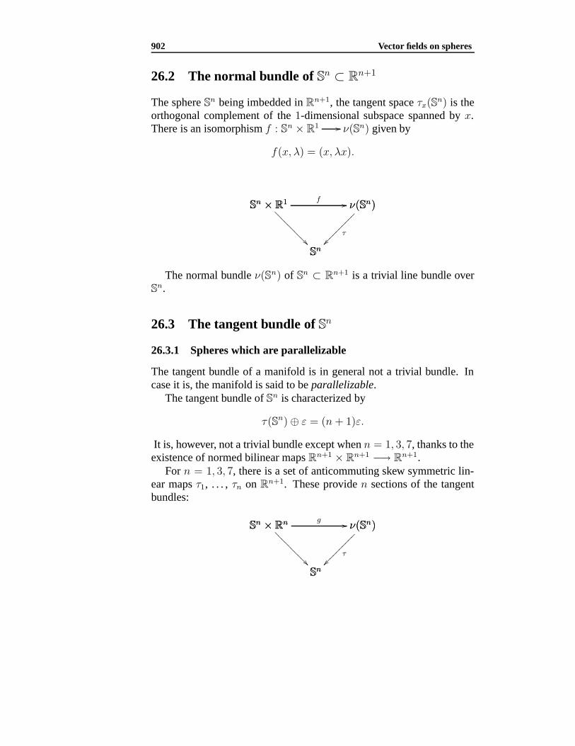
902 Vector fields on spheres
26.2 The normal bundle of Sn ⊂ Rn+1
The sphere Sn being imbedded in Rn+1, the tangent space τx(Sn) is the
orthogonal complement of the 1-dimensional subspace spanned by x.There is an isomorphism f : Sn × R1 ν(Sn) given by
f(x, λ) = (x, λx).
Sn × R1
Sn
Sn × R1 ν(Sn)f ν(Sn)
Sn
τ
The normal bundle ν(Sn) of Sn ⊂ Rn+1 is a trivial line bundle overSn.
26.3 The tangent bundle of Sn
26.3.1 Spheres which are parallelizable
The tangent bundle of a manifold is in general not a trivial bundle. Incase it is, the manifold is said to be parallelizable.
The tangent bundle of Sn is characterized by
τ(Sn)⊕ ε = (n + 1)ε.
It is, however, not a trivial bundle except when n = 1, 3, 7, thanks to theexistence of normed bilinear maps Rn+1 × Rn+1 −→ Rn+1.
For n = 1, 3, 7, there is a set of anticommuting skew symmetric lin-ear maps τ1, . . . , τn on Rn+1. These provide n sections of the tangentbundles:
Sn × Rn
Sn
Sn × Rn ν(Sn)g ν(Sn)
Sn
τ
26.3 The tangent bundle of Sn 903
g(x, t1, . . . , tn) := t1τ1(x) + · · ·+ tnτn(x).
The nontriviality of τ(Sn) is a deep theorem proved in the late 1950’s.
THEOREM (Kervaire-Milnor). The sphere Sn is parallelizable if andonly if n = 1, 3, 7.
26.3.2 The hairy ball theorem
Theorem 26.1. If n is even, there is no nonzero vector field on Sn.
Proof. Suppose Sn admits a nonzero vector field. We may assume itis a unit tangent vector field τ(x), so that (x, τ(x)) are orthogonal unitvectors for every x ∈ Sn. Consider the homotopy ht : Sn Sn givenby
ht(x) = x · cos tπ + τ(x) · sin tπ.
Clearly, h0 is the identity map on Sn. On the other hand, h1 is theantipodal map. These two maps being homotopic, they should have thesame degree. It follows that 1 = (−1)n+1 and n must be odd.
26.3.3 Linearly independent tangent vector fields on Sn
For odd values of n, the tangent bundle of Sn may contain trivial sub-
bundles.
THEOREM (Adams). The maximum number of linearly independenttangent vector fields on Sn is ρ(n + 1)− 1.

904 Vector fields on spheres
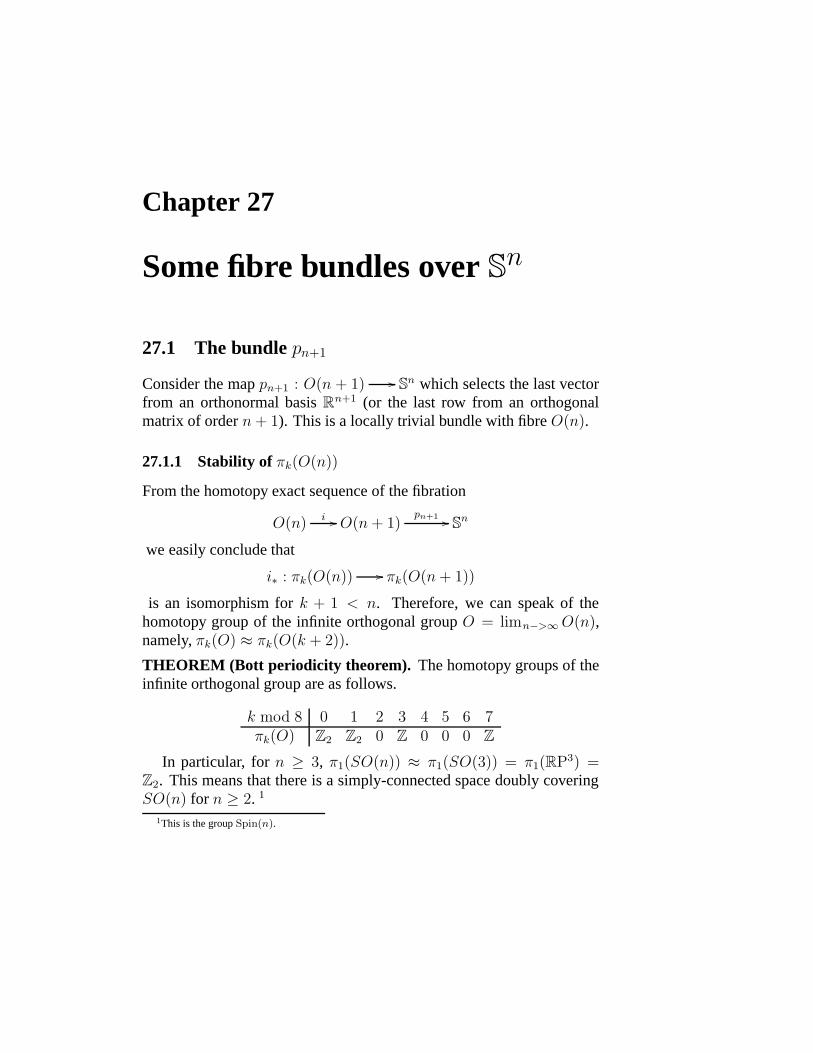
Chapter 27
Some fibre bundles over Sn
27.1 The bundle pn+1
Consider the map pn+1 : O(n + 1) Sn which selects the last vectorfrom an orthonormal basis Rn+1 (or the last row from an orthogonalmatrix of order n+ 1). This is a locally trivial bundle with fibre O(n).
27.1.1 Stability of πk(O(n))
From the homotopy exact sequence of the fibration
O(n) i O(n+ 1)pn+1 Sn
we easily conclude that
i∗ : πk(O(n)) πk(O(n+ 1))
is an isomorphism for k + 1 < n. Therefore, we can speak of thehomotopy group of the infinite orthogonal group O = limn−>∞ O(n),namely, πk(O) ≈ πk(O(k + 2)).
THEOREM (Bott periodicity theorem). The homotopy groups of theinfinite orthogonal group are as follows.
k mod 8 0 1 2 3 4 5 6 7πk(O) Z2 Z2 0 Z 0 0 0 Z
In particular, for n ≥ 3, π1(SO(n)) ≈ π1(SO(3)) = π1(RP3) =Z2. This means that there is a simply-connected space doubly coveringSO(n) for n ≥ 2. 1
1This is the group Spin(n).

906 Some fibre bundles over Sn
27.1.2 Cross sections of pn+1
A cross section of the bundle pn+1 is a map s : Sn O(n+1) such thats pn+1 = ιSn . This is equivalent to a continuous orthonormal frame ofthe tangent bundle of Sn. If such a framing is possible, we say that thesphere Sn is parallelizable. 2
27.2 Stiefel manifolds
The Stiefel manifold Vn,k is the space of orthonormal k-frames in Rn:
Vn,k := (v1, . . . , vk) : v1, . . . , vk are mutually orthogonal unit vectors in Rn.
It can also be regarded as the subspaces of k × n real matrices A satis-fying AAt = Ik.
There is a fibre bundle
Vn, k Vn+1, k+1
pn+1,k+1 Sn
in which the map pn+1,k+1 selects the last vector from an orthonormal(k + 1)-frame in Rn+1.
From the homotopy exact sequence, we have isomorphisms
i∗ : πm(Vn, k) πm(Vn+1, k+1)
for m+ 1 < n.A cross section of the bundle pn+1,k+1 is equivalent to k linearly in-
dependent tangent vector fields on Sn. 3
27.3 Characteristic element of a bundle over Sn
Consider a bundle p : E Sn with fibre F . From the homotopy exactsequence, we easily conclude that the injection i∗ : πk(F ) πk(E) isan isomorphism for k < n − 1 and an epimorphism for k = n − 1. 4
From
· · · πn(Sn)
∆∗ πn−1(F )i∗ πn−1(E) 0,
2See the Kervaire-Milnor theorem (Theorem 26.3.1) in §26.3See Adams’ theorem (Theorem 26.3.3) in §264This fact is often summarized by saying that i : F E is an n-equivalence.
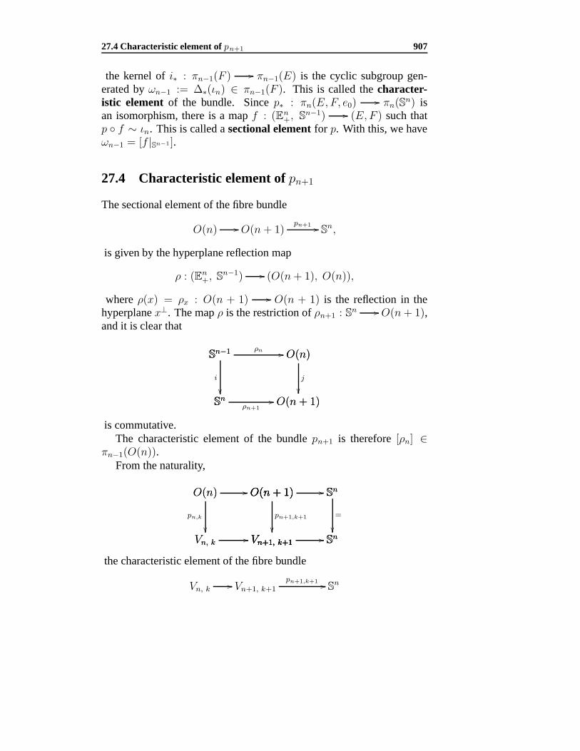
27.4 Characteristic element of pn+1 907
the kernel of i∗ : πn−1(F ) πn−1(E) is the cyclic subgroup gen-erated by ωn−1 := ∆∗(ιn) ∈ πn−1(F ). This is called the character-istic element of the bundle. Since p∗ : πn(E,F, e0) πn(S
n) isan isomorphism, there is a map f : (En
+, Sn−1) (E,F ) such thatp f ∼ ιn. This is called a sectional element for p. With this, we haveωn−1 = [f |Sn−1].
27.4 Characteristic element of pn+1
The sectional element of the fibre bundle
O(n) O(n+ 1)pn+1 Sn,
is given by the hyperplane reflection map
ρ : (En+, S
n−1) (O(n+ 1), O(n)),
where ρ(x) = ρx : O(n + 1) O(n + 1) is the reflection in thehyperplane x⊥. The map ρ is the restriction of ρn+1 : Sn O(n+ 1),and it is clear that
Sn O(n+ 1)ρn+1
Sn−1
Sn
i
Sn−1 O(n)ρn O(n)
O(n+ 1)
j
is commutative.The characteristic element of the bundle pn+1 is therefore [ρn] ∈
πn−1(O(n)).From the naturality,
Vn, k Vn+1, k+1
O(n)
Vn, k
pn,k
O(n) O(n+ 1) O(n+ 1)
Vn+1, k+1
pn+1,k+1
Vn+1, k+1 Sn
O(n+ 1)
Vn+1, k+1
O(n+ 1) Sn Sn
Sn
=
the characteristic element of the fibre bundle
Vn, k Vn+1, k+1
pn+1,k+1 Sn

908 Some fibre bundles over Sn
is the homotopy class of
ρn,k = pn,k ρn : Sn−1 Vn, k
in πn−1(Vn, k).
Proposition 27.1. The sphere Sn admits k linearly independent tangentvector fields if and only if ρn,k : Sn−1 Vn, k is trivial.
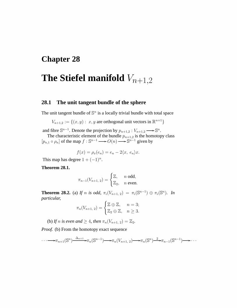
Chapter 28
The Stiefel manifold Vn+1,2
28.1 The unit tangent bundle of the sphere
The unit tangent bundle of Sn is a locally trivial bundle with total space
Vn+1,2 := (x, y) : x, y are orthogonal unit vectors in Rn+1
and fibre Sn−1. Denote the projection by pn+1,2 : Vn+1,2 Sn.
The characteristic element of the bundle pn+1,2 is the homotopy class[pn,1 ρn] of the map f : Sn−1 O(n) Sn−1 given by
f(x) = ρx(en) = en − 2〈x, en〉x.This map has degree 1 + (−1)n.
Theorem 28.1.
πn−1(Vn+1, 2) =
Z, n odd,
Z2, n even.
Theorem 28.2. (a) If n is odd, πi(Vn+1, 2) = πi(Sn−1) ⊕ πi(S
n). Inparticular,
πn(Vn+1, 2) =
Z ⊕ Z, n = 3;
Z2 ⊕ Z, n ≥ 3.
(b) If n is even and ≥ 4, then πn(Vn+1, 2) = Z2.
Proof. (b) From the homotopy exact sequence
· · · πn+1(Sn)
∆n+1 πn(Sn−1) πn(Vn+1, 2) πn(S
n) 2 πn−1(Sn−1) · · ·
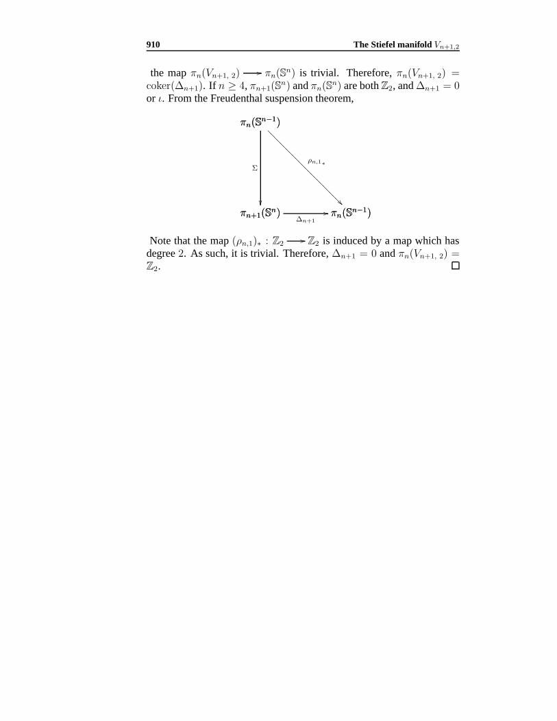
910 The Stiefel manifold Vn+1,2
the map πn(Vn+1, 2) πn(Sn) is trivial. Therefore, πn(Vn+1, 2) =
coker(∆n+1). If n ≥ 4, πn+1(Sn) and πn(S
n) are both Z2, and ∆n+1 = 0or ι. From the Freudenthal suspension theorem,
πn+1(Sn) πn(S
n−1)∆n+1
πn(Sn−1)
πn+1(Sn)
Σ
πn(Sn−1)
πn(Sn−1)
ρn,1∗
Note that the map (ρn,1)∗ : Z2 Z2 is induced by a map which has
degree 2. As such, it is trivial. Therefore, ∆n+1 = 0 and πn(Vn+1, 2) =Z2.