Algebraic Topology

DRAFT 2013 - U.T.

Contents

0 Introduction 2

1 Chain complexes 2

2 Simplicial homology 4

3 Singular homology 6

4 Chain homotopy and homotopy invariance 84.1 Chain homotopy . . . . . . . . . . . . . . . . . . . . . . . . . . . . . . . . . . . . . . . 84.2 Homotopy invariance . . . . . . . . . . . . . . . . . . . . . . . . . . . . . . . . . . . . 9

5 The Snake Lemma and relative homology 10

6 The Five Lemma and excision 126.1 A tool . . . . . . . . . . . . . . . . . . . . . . . . . . . . . . . . . . . . . . . . . . . . . 126.2 Excision . . . . . . . . . . . . . . . . . . . . . . . . . . . . . . . . . . . . . . . . . . . . 136.3 Locality . . . . . . . . . . . . . . . . . . . . . . . . . . . . . . . . . . . . . . . . . . . . 146.4 Mayer-Vietoris sequence . . . . . . . . . . . . . . . . . . . . . . . . . . . . . . . . . . . 15

7 The degree of a map of spheres 15

8 Cellular homology 17

9 Cohomology and the Universal Coefficient Theorem 209.1 Cohomology . . . . . . . . . . . . . . . . . . . . . . . . . . . . . . . . . . . . . . . . . . 209.2 Universal Coefficient Theorem . . . . . . . . . . . . . . . . . . . . . . . . . . . . . . . 21

10 The Kunneth Theorem and products 2310.1 Algebraic Kunneth formula . . . . . . . . . . . . . . . . . . . . . . . . . . . . . . . . . 2310.2 The cup product . . . . . . . . . . . . . . . . . . . . . . . . . . . . . . . . . . . . . . . 2310.3 Product spaces . . . . . . . . . . . . . . . . . . . . . . . . . . . . . . . . . . . . . . . . 25

11 Manifolds and fundamental classes 26

12 Duality 2812.1 Poincare duality . . . . . . . . . . . . . . . . . . . . . . . . . . . . . . . . . . . . . . . 2812.2 Leftschetz duality . . . . . . . . . . . . . . . . . . . . . . . . . . . . . . . . . . . . . . 2912.3 Alexander duality . . . . . . . . . . . . . . . . . . . . . . . . . . . . . . . . . . . . . . 29

1

0 Introduction

We study topological spaces by associating algebraic objects which are invariant under homotopy(deformation).

Sets: number of path components π0

Numbers: Euler characteristic χwinding number w(γ)

Groups: fundamental group π1

Graded abelian groups: Homology H∗Graded rings: Cohomology H∗

This course will introduce and study homology and cohomology.

Why?

• Nonabelian groups are difficult to work with

• π1 only tells us something about the 2-skeleton of a space

• higher dimensional analogues, πn = {homotopy classes of based maps from Sn to the spaceof interest}, are very hard to compute. Even πn(Sk) are not all know for n > k.

Homology, H∗, is a refinement of the Euler characteristic and still relatively easy to compute.

References

Everything contained in this course is covered in

• chapters 2 and 3 of ‘Algebraic Topology’ by Allen Hatcher, available online athttp://www.math.cornell.edu/∼hatcher/

1 Chain complexes

Definition 1.1. Let C0,C1, . . . be abelian groups (or vector spaces) and let ∂n ∶ Cn → Cn−1 behomomorphisms (or linear maps). Assume that ∂n ○ ∂n+1 = 0 for all n. Then

(C●, ∂●) ..= ⋯ ∂3ÐÐ→ C2∂2ÐÐ→ C1

∂1ÐÐ→ C0∂0=0ÐÐÐ→ 0

is a chain complex. Furthermore define

• n-chains: Cn

• n-cycles: Zn ..= ker(∂n)

• n-boundaries: Bn ..= im(∂n+1)

Sometimes we refer to a chain complex as C● for simplicity.

Note 1.2. As ∂n ○ ∂n+1 = 0, Bn ⊆ Zn.

2

Definition 1.3. The n-th homology of a chain complex (C●, ∂●) is

Hn(C●, ∂●) ..= Zn/Bn = ker(∂n)/ im(∂n+1).

C● is called exact at Cn if Hn = 0, i.e. if ker(∂n) = im(∂n+1). C● is called exact if it is exact atCn for all n ≥ 0.

Example 1.4. Let

0Ð→ AαÐÐ→ B

βÐÐ→ C Ð→ 0

be a short exact sequence of abelian groups, then

ker(α) = im(0) = {0}ker(β) = im(α) = Aker(0) = C = im(β)

Ô⇒ α is injective

Ô⇒ β is surjective

Thus C is isomorphic to the quotient B/A. Note that the group B is not determined by A andC. For example, when A = Z and C = Z/2Z then B could be Z or Z⊕Z/2Z. On the otherhand,if in a short exact sequence of vector spaces where A, B and C are finite dimensional and allmaps are linear, B is determined by A and C upto isomorphism: dim(B) = dim(A) + dim(C).

Definition 1.5. A chain map φ ∶ (C●, ∂●)→ (C●, ∂●) is a collection of homomorphisms φn ∶ Cn → Cnsuch that the following diagram commutes.

⋯ // C2∂2 //

φ2��

C1∂1 //

φ1��

C0∂0 //

φ0��

0

⋯ // C2

∂2 // C1

∂1 // C0

∂0 // 0

That is, such that φn−1 ○ ∂n = ∂n ○ φn for all n ≥ 0.

Proposition 1.6. φ ∶ C● → C● induces a homomorphism φ∗ ∶ Hn(C●) → Hn(C●) for all n ≥ 0

by φ∗([x]) = [φn(x)] where [x] = x +Bn ∈ Zn/Bn =Hn(C●).

Proof. We show that the map is well-defined:Let [x] = [x′], then x = x′ + b for some b ∈ Bn. So φn(x) = φn(x′ + b) = φn(x′) + φn(b). We needφn(b) ∈ Bn, then [φn(x)] = [φn(x′)].

Cn+1

φn+1

��

∂n+1 //

b′� //

Cn

φn

��

∂n //

b_

��

Cn−1

φn−1

��

Cn+1

∂n+1 // Cn∂n //

φn(b)Cn−1

Since b ∈ Bn, there is a b′ ∈ Cn+1 such that ∂n+1(b′) = b.Then, by commutativity,

φn(b) = φn(∂n+1(b′))= ∂n+1 ○ φn+1(b′)∈ Bm = im(∂n+1).

Finally, one checks that φn(x) ∈ Zn: as x is a cycle, ∂n ○ φn(x) = φn−1 ○ ∂n(x) = 0.

We will study three different notions of homology groups Hn(X) for a topological space X,which will agree when defined.

3

Simplicial Homology easy to compute and good geometric intuitionSingular Homology good for theoretical workCellular Homology better for computations and applications

Through out the course we will use freely the following result from algebra.

Theorem 1.7. Any finitely generated abelian group is isomorphic to

Zr ⊕ (Z/pn11 Z)⊕ (Z/pn2

2 Z)⊕⋯⊕ (Z/pnkk Z)

for some r ∈ Z≥0, k ∈ Z≥0, each pi is prime (possibly with pi = pj for i ≠ j) and each ni ∈ Z>0.Moreover, r, k, pi and ni are unique up to reordering.

Example 1.8. (1) Z/6Z ≅ Z/2Z⊕Z/3Z(2) Z/9Z ≇ Z/3Z⊕Z/3Z

2 Simplicial homology

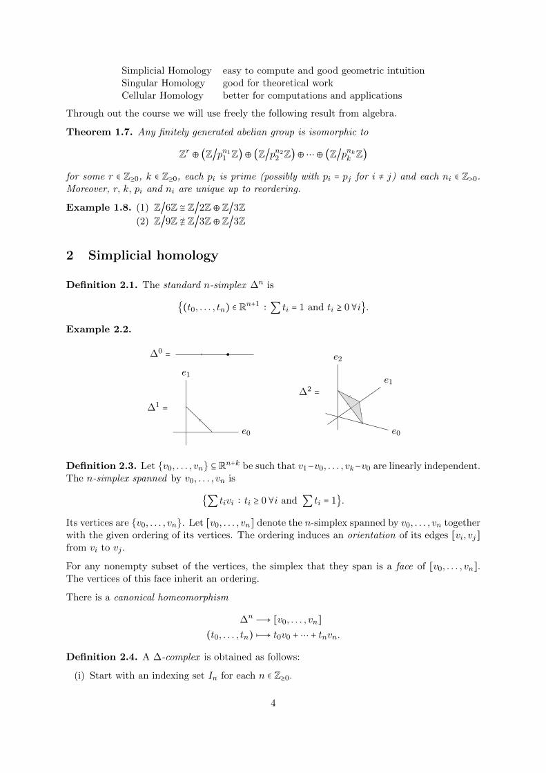
Definition 2.1. The standard n-simplex ∆n is

{(t0, . . . , tn) ∈ Rn+1 ∶ ∑ ti = 1 and ti ≥ 0∀i}.

Example 2.2.

∆0 =

∆1 =

e0

e1

∆2 =

e2

e1

e0

Definition 2.3. Let {v0, . . . , vn} ⊆ Rn+k be such that v1−v0, . . . , vk−v0 are linearly independent.The n-simplex spanned by v0, . . . , vn is

{∑ tivi ∶ ti ≥ 0∀i and ∑ ti = 1}.

Its vertices are {v0, . . . , vn}. Let [v0, . . . , vn] denote the n-simplex spanned by v0, . . . , vn togetherwith the given ordering of its vertices. The ordering induces an orientation of its edges [vi, vj]from vi to vj .

For any nonempty subset of the vertices, the simplex that they span is a face of [v0, . . . , vn].The vertices of this face inherit an ordering.

There is a canonical homeomorphism

∆n Ð→ [v0, . . . , vn](t0, . . . , tn)z→ t0v0 +⋯ + tnvn.

Definition 2.4. A ∆-complex is obtained as follows:

(i) Start with an indexing set In for each n ∈ Z≥0.

4

(ii) For each α ∈ In take a copy σnα of the standard n-simplex.

(iii) Form the disjoint union of all these simplices over all n ∈ Z≥0: ∐n∈Z≥0∐α∈In σnα.

(iv) We require that for each (n−1)-dimensional face of each n-simplex σnα there is an associated(n − 1)-simplex σn−1

β for some β ∈ In−1.

(v) Form the quotient space by identifying each (n − 1)-dimensional face of each σnα with theassociated simplex σn−1

β using the canonical homeomorphism. These homeomorphismspreserve the ordering of the vertices.

Example 2.5. The torus admits the structure of a ∆-complex with

one 0-simplexthree 1-simplicestwo 2-simplices

Note 2.6. The following is not a well-defined ∆-complex becausethe vertices of each 2-simplex are not totally ordered.

Remark 2.7. Any simplicial complex is a ∆-complex, but in a ∆-complex an n-simplex may notbe uniquely determined by its vertices as in Example 2.5.

Definition 2.8. Let X● be a ∆-complex. The n-th chain group C∆n (X●) of X● is the free abelian

group generated by the set of n-simplices Xn of X●. An element of C∆n (X●) is ∑α∈In cασ

nα, where

each cα ∈ Z and only finitely many of the cα’s are non-zero. The boundary homomorphism is

∂n ∶ C∆n (X●)Ð→ C∆

n−1(X●)[v0, . . . , vn]z→∑

i

(−1)i[v0, . . . , vi, . . . , vn]

where [v0, . . . , vi, . . . , vn] ..= [v0, . . . , vi−1, vi+1, . . . , vn].

Example 2.9.

∂1

⎛⎜⎝ v0

v1 ⎞⎟⎠=⎛⎜⎝ −v0

+v1 ⎞⎟⎠

∂2

⎛⎜⎜⎜⎝ v0 v1

v2 ⎞⎟⎟⎟⎠=⎛⎜⎜⎝ ×1

×−1 ×1 ⎞⎟⎟⎠

Key Lemma 2.10. ∂n−1 ○ ∂n = 0 ∀n

Proof.

∂n−1 ○ ∂n([v0, . . . , vn]) = ∂n−1(∑i

(−1)i[v0, . . . , vi, . . . , vn])

=∑j<i

(−1)i(−1)j[v0 . . . , vj , . . . , vi, . . . , vn]

+∑j>i

(−1)i(−1)j−1[v0 . . . , vi, . . . , vj , . . . , vn]

= 0.

5

Definition 2.11. For n ≥ 0 the n-th simplicial homology group H∆n (X●) is the n-th homology

group of the chain complex

⋯Ð→ C∆n+1(X●)

∂n+1ÐÐ→ C∆n (X●)

∂nÐÐ→ C∆n−1(X●)Ð→ ⋯

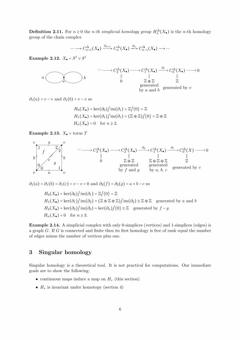
Example 2.12. X● = S1 ∨ S1

av

b

⋯ // C∆2 (X●) // C∆

1 (X●)∂1 // C∆

0 (X●) // 0

0 Z⊕Z Zgeneratedby a and b

generated by v

∂1(a) = v − v and ∂1(b) = v − v so

H0(X●) = ker(∂0)/ im(∂1) = Z/{0} = ZH1(X●) = ker(∂1)/ im(∂1) = (Z⊕Z)/{0} = Z⊕ZHn(X●) = 0 for n ≥ 2.

Example 2.13. X● = torus T

v

v

v

v

b b

a

a

c

00

1

1 22

g

f⋯ // C∆

3 (X●) // C∆2 (X●)

∂2 // C∆1 (X●)

∂1 // C∆0 (X) // 0

0 Z⊕Z Z⊕Z⊕Z Zgeneratedby f and g

generatedby a, b, c

generated by v

∂1(a) = ∂1(b) = ∂1(c) = v − v = 0 and ∂2(f) = ∂2(g) = a + b − c so

H0(X●) = ker(∂0)/ im(∂1) = Z/{0} = ZH1(X●) = ker(∂1)/ im(∂2) = (Z⊕Z⊕Z)/ im(∂2) ≅ Z⊕Z generated by a and b

H2(X●) = ker(∂2)/ im(∂3) = ker(∂n)/{0} ≅ Z generated by f − gHn(X●) = 0 for n ≥ 3.

Example 2.14. A simplicial complex with only 0-simplices (vertices) and 1-simplices (edges) isa graph G. If G is connected and finite then its first homology is free of rank equal the numberof edges minus the number of vertices plus one.

3 Singular homology

Singular homology is a theoretical tool. It is not practical for computations. Our immediategoals are to show the following:

• continuous maps induce a map on H∗ (this section)

• H∗ is invariant under homotopy (section 4)

6

Definition 3.1. Let X be a topological space. A continuous map σ ∶ ∆n = [e0, . . . , en] → X iscalled a singular n-simplex. The singular n-chains are the elements of the free abelian groupgenerated by the n-simplices:

Cn(X) ..= {∑α

aασα ∶ aα ∈ Z with only finitely many ≠ 0, σα ∶ ∆n →X}

The boundary operator is defined on generators by

∂n ∶ Cn(X)Ð→ Cn−1(X)

σ z→ ∂nσ ..=n

∑i=0

(−1)iσ∣[e0,...,ei,...,en]

Lemma 3.2. ∂n−1 ○ ∂n = 0 ∀n

Proof. Heuristically, ∂n restricts a singular simplex σ to its boundary ∂n[e0, . . . , en]. The bound-ary has no boundary. So ∂n−1(∂nσ) restricts σ restricted to the empty set and ∂n−1(∂n[e0, . . . , en]) = 0.For a formal proof imitate the proof of Key Lemma in section 2.

Definition 3.3. Singular homology Hn(X) ..=Hn(C●(X)).

Remark 3.4. For a simplicial complex X●, the map that assigns to an n-simplex α its canon-ical homeomorphism σα ∶ ∆n → α induces a chain map C∆

● (X●) → C●(X) which induces anisomorphism of homology groups as we will see later.

Example 3.5. X = pt. For each n there is only one map cn ∶ ∆n →X.

∂n(cn) =n

∑i=0

(−1)icn∣[e0,...,ei,...,en]

=⎧⎪⎪⎨⎪⎪⎩

0 if n is odd

cn−1 if n is even

Ô⇒ C● = ⋯1Ð→ Z 0Ð→ Z 1Ð→ Z 0Ð→ Z 0Ð→ 0

Ô⇒ Hn(pt) =⎧⎪⎪⎨⎪⎪⎩

Z n = 0

0 n ≠ 0

Naturality. Let f ∶X → Y be a continuous maps. Define

f♯ ∶ Cn(X)Ð→ Cn(Y )σ z→ f ○ σ ∶ ∆n →X → Y.

Note that ∂n ○ f♯(σ) = f♯ ○ ∂n(σ). Hence f♯ induces a map of chain complexes and hence ahomomorphism of homology groups:

f∗ ∶Hn(X)Ð→Hn(Y ) for all n.

Furthermore, if g ∶ Y → Z is another continuous map then

(g ○ f)♯ = g♯ ○ f♯ and (g ○ f)∗ = g∗ ○ f∗(idX)♯ = idC●(X) and (idX)∗ = idHn for all n

where idX ∶X →X is the identity map.

7

Aside 3.6. ( Optional) This says that homology is a functor from the category of topologicalspaces and continuous maps to the category of graded abelian groups and homomorphisms thatpreserve the grading:

X z→H∗(X) =⊕n≥0

Hn(X).

4 Chain homotopy and homotopy invariance

We will first establish a criterion (chain homotopy) for when two chain maps induce the samehomomorphism in homology. Then we will show that a homotopy between two continuous mapsinduces such a chain homotopy and hence the two maps induce the same homomorphism inhomology.

4.1 Chain homotopy

Definition 4.1. Two maps of chain complexes φ●, ψ● ∶ (C●, ∂●)→ (C●, ∂●) are chain homotopic

if there exist homomorphisms hn ∶ Cn → Cn+1 such that

∂n+1 ○ hn + hn−1 ○ ∂n = φn − ψn.

h● is called a chain homotopy.

Proposition 4.2. If φ● and ψ● are chain homotopic then

φ∗ = ψ∗ ∶Hn(C●)Ð→Hn(C●).

Proof. Let z ∈ Zn = ker∂n. Then

φn(z) − φn(z) = (∂n+1 ○ hn + hn−1 ○ ∂n)(z) as z ∈ Zn= (∂n+1 ○ hn)(z) ∈ Bn = im ∂n+1.

Hence, φ∗([z]) = [φn(z)] = [ψn(z)] = ψ∗([z]).

Cn+1// Cn

hn

yyssssssssss

φ−ψ��

∂n // Cn−1

hn−1yysssssssssss

Cn+1∂n+1

// Cn// Cn−1

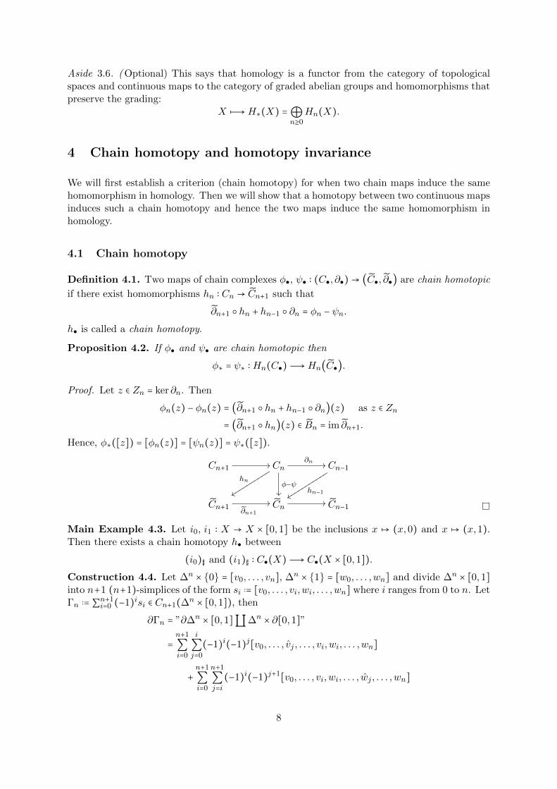
Main Example 4.3. Let i0, i1 ∶ X → X × [0,1] be the inclusions x ↦ (x,0) and x ↦ (x,1).Then there exists a chain homotopy h● between

(i0)♯ and (i1)♯ ∶ C●(X)Ð→ C●(X × [0,1]).

Construction 4.4. Let ∆n × {0} = [v0, . . . , vn], ∆n × {1} = [w0, . . . ,wn] and divide ∆n × [0,1]into n+1 (n+1)-simplices of the form si ..= [v0, . . . , vi,wi, . . . ,wn] where i ranges from 0 to n. LetΓn ..= ∑n+1

i=0 (−1)isi ∈ Cn+1(∆n × [0,1]), then

∂Γn = ”∂∆n × [0,1]∐∆n × ∂[0,1]”

=n+1

∑i=0

i

∑j=0

(−1)i(−1)j[v0, . . . , vj , . . . , vi,wi, . . . ,wn]

+n+1

∑i=0

n+1

∑j=i

(−1)i(−1)j+1[v0, . . . , vi,wi, . . . , wj , . . . ,wn]

8

Terms i = j cancel except for [w0, . . . ,wn] − [v0, . . . , vn]. Terms i ≠ j are ”Γ(∂∆n × [0,1])”.

v0 v1

w0 w1

ÿ

⟲

Γ1 = [v0,w0,w1] − [v0, v1,w1]

∂Γ1 = [w0,w1] −����[v0,w1] + [v0,w0]− [v1,w1] +����[v0,w1] − [v0, v1]

Let (σ ∶ ∆n →X) ∈ Cn(X) and σ × 1 ∶ ∆n × [0,1]→X × [0,1], (x, t)↦ (σ(x), t). Define

h ∶ Cn(X)Ð→ Cn+1(X × [0,1])σ z→ (σ × 1)♯(Γn)

Then

∂h(σ) = ∂(σ × 1)♯(Γn)= (σ × 1)♯∂(Γn)= (i1)♯(σ) − h∂(σ) − (i0)♯(σ)

and so ∂●h● + h●∂● = (i1)♯ − (i0)♯.

4.2 Homotopy invariance

Definition 4.5. Two continuous maps f0, f1 ∶X → Y are homotopic if there exists a continuousmap

F ∶X × [0,1]Ð→ Y such thatF (x,0) = f0(x)F (x,1) = f1(x).

F is called a homotopy and we write f0 ∼ f1. If A is a subset of X and f0∣A = f1∣A and thehomotopy F satisfies F (x, t) = f0(x) = f1(x) for all x ∈ A and all t ∈ [0,1], then f0 and f1 aresaid to be homotopic relative to A.

Note 4.6. Homotopy is an equivalence relation.

Definition 4.7. Two spaces X and Y are homotopy equivalent if there exist maps

f ∶X Ð→ Y

g ∶ Y Ð→Xsuch that

g ○ f ∼ idX

f ○ g ∼ idY .

X is called contractible if it is homotopy equivalent to a point.

Example 4.8. Rn is contractible. f ∶ Rn → ∗, g ∶ ∗→ 0 ∈ Rn. Then f ○ g = id∗ and

F ∶ Rn × [0,1]Ð→ Rn

(x, t)z→ txwith

F (x,0) = 0 = g ○ f(x)F (x,1) = x = idRn(x)

Theorem 4.9 (Homotopy invariance). If f0 ∼ f1, then (f0)∗ = (f1)∗ ∶Hn(X)→Hn(Y ).

9

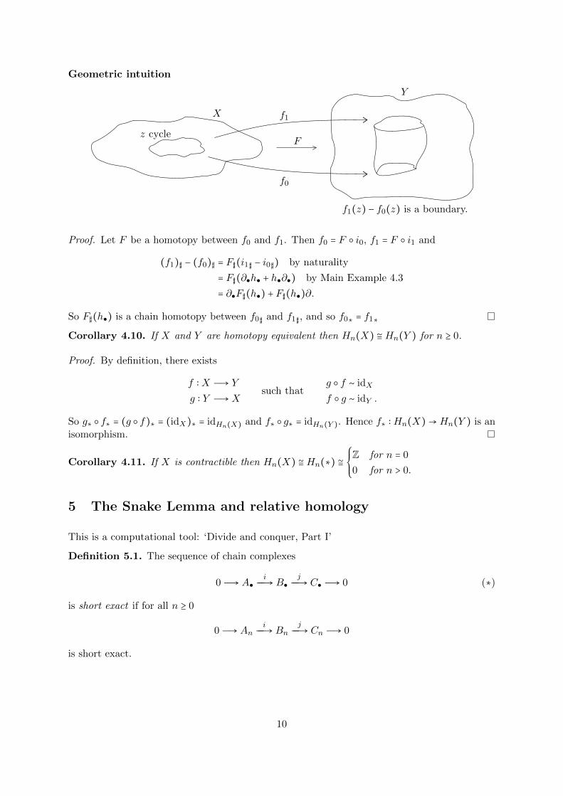
Geometric intuition

z cycle

f1

f0

X

Y

F

f1(z) − f0(z) is a boundary.

Proof. Let F be a homotopy between f0 and f1. Then f0 = F ○ i0, f1 = F ○ i1 and

(f1)♯ − (f0)♯ = F♯(i1♯ − i0♯) by naturality

= F♯(∂●h● + h●∂●) by Main Example 4.3

= ∂●F♯(h●) + F♯(h●)∂.

So F♯(h●) is a chain homotopy between f0♯ and f1♯, and so f0∗ = f1∗

Corollary 4.10. If X and Y are homotopy equivalent then Hn(X) ≅Hn(Y ) for n ≥ 0.

Proof. By definition, there exists

f ∶X Ð→ Y

g ∶ Y Ð→Xsuch that

g ○ f ∼ idX

f ○ g ∼ idY .

So g∗ ○ f∗ = (g ○ f)∗ = (idX)∗ = idHn(X) and f∗ ○ g∗ = idHn(Y ). Hence f∗ ∶Hn(X)→Hn(Y ) is anisomorphism.

Corollary 4.11. If X is contractible then Hn(X) ≅Hn(∗) ≅⎧⎪⎪⎨⎪⎪⎩

Z for n = 0

0 for n > 0.

5 The Snake Lemma and relative homology

This is a computational tool: ‘Divide and conquer, Part I’

Definition 5.1. The sequence of chain complexes

0Ð→ A●iÐÐ→ B●

jÐÐ→ C● Ð→ 0 (∗)

is short exact if for all n ≥ 0

0Ð→ AniÐÐ→ Bn

jÐÐ→ Cn Ð→ 0

is short exact.

10

Theorem 5.2 (The Snake Lemma). Given a short exact sequence of chain complexes (∗) thereexist connecting homomorphisms

δ ∶Hn(C●)Ð→Hn−1(A●)

such that the following sequence is long exact:

⋯ δÐÐ→Hn(A●)i∗ÐÐ→Hn(B●)

j∗ÐÐ→Hn(C●)δÐÐ→Hn−1(A●)Ð→ ⋯Ð→H0(B●)Ð→H0(C●)Ð→ 0

Proof. Definition of δ:Let c ∈ Zn(C●). Since j is a surjection there exists b ∈ Bn such that j(b) = c. Then ∂b ∈ Bn−1

and j(∂b) = ∂j(b) = ∂c = 0. By exactness there exists a ∈ An−1 such that i(a) = ∂b. Defineδ[c] ..= [a].

Well-defined:

(1) a is a cycle: i(∂a) = ∂(i(a)) = ∂(∂b) = 0, and so ∂a = 0 as i is injective.

(2) Independence of choice of c: assume [c] = [c′]

b′′ //

��

b − b′ + i(e)

��

c′′ // c − c′

Ô⇒ c′ − c = ∂c′′ and c′′ = j(b′′)Ô⇒ ∂b′′ = b − b′ + i(e) and as ∂∂b′′ = 0

Ô⇒ ∂i(e)) = i(∂e) = ∂b − ∂b′ = ia − ia′

Ô⇒ [a] = [a′] ∈Hn−1(A●).

Exactness at Hn(C●): im j∗ ⊆ ker δ: let [c] ∈ im j∗, then there exists b such that j∗[b] = [c]. Inparticular ∂b = 0 so if i(a) = ∂b then a = 0 so δ[c] = 0.im j∗ ⊇ ker δ: let δ[c] = [a] = 0

a′ // a

��

b //

��

∂b

��

c // 0

Ô⇒ ∃a′ ∶ ∂a′ = aÔ⇒ ∂ia′ = i∂a′ = ia = ∂b where jb = cput b′ = b − ia′

note jb′ = jb − jia′ = jb = cÔ⇒ ∂b′ = ∂b − ∂ia′ = ∂b − ∂b = 0

Ô⇒ [c] = [jb′] = j∗[b′].Exactness at Hn(A●) and Hn(B●) follow in a similar way.

Note 5.3. If A● ⊂ B● and C● = B●/A● with ∂(b +An) = ∂b +An−1 then δ[b +An] = [∂b].

Let (X,A) be a pair of spaces, i.e. a space X and a subspace A. Then the inclusion A ↪ Xinduces an inclusion of chain complexes C●(A)↪ C●(X). Define the relative homology of (X,A)as

Hn(X,A) ..=Hn(C●(X)/C●(A)).

Note 5.4. A cycle in C●(X,A) ..= C●(X)/C●(A) is a chain x ∈ Cn(X) with ∂x ∈ Cn−1(A) andδ[x] = [∂x].

A

11

It will be convenient to introduce the reduced homology of a space, which is defined to beHn(X) ..= ker(Hn(X)→Hn(pt)). Note that Hn(X) = Hn(X) for n > 0. Furthermore, acontinuous map f ∶X → Y defines a map of reduced homology groups.

Corollary 5.5. There is a long exact sequence in reduced homology

⋯Ð→ H1(A)Ð→ H1(X)Ð→ H1(X,A) δÐÐ→ H0(A)Ð→ H0(X)Ð→H0(X,A)Ð→ 0.

Proof. By the Snake Lemma

⋯Ð→H1(X,A) δÐÐ→H0(A)Ð→H0(X)Ð→H0(X,A)Ð→ 0

is exact. It is an exercise to show that H0(A) → H0(X), and that A ↪ X maps Z ≅Ð→ Zin H0(A) = H0(A) ⊕ Z and H0(X) = H0(X) ⊕ Z. So the sequence in reduced homology isexact.

Example 5.6. (X,A) = (Dk, Sk−1). Note Dk ≃ ∗ and so Hn(X) = 0 for all n ≥ 0 so

Hn(Dk, Sk−1) ≅ Hn−1(Sk−1)

for all n ≥ 0.

Let (X,A) and (Y,B) be two pairs of spaces. A map of pairs of spaces is a continuous mapf ∶X → Y such that f(A) ⊂ B.

Proposition 5.7. A map of pairs of spaces induces a map of long exact sequences.

Proof. This is left as an exercise.

6 The Five Lemma and excision

Excision distinguishes homology from homotopy and makes the former more accessible to com-putations.

6.1 A tool

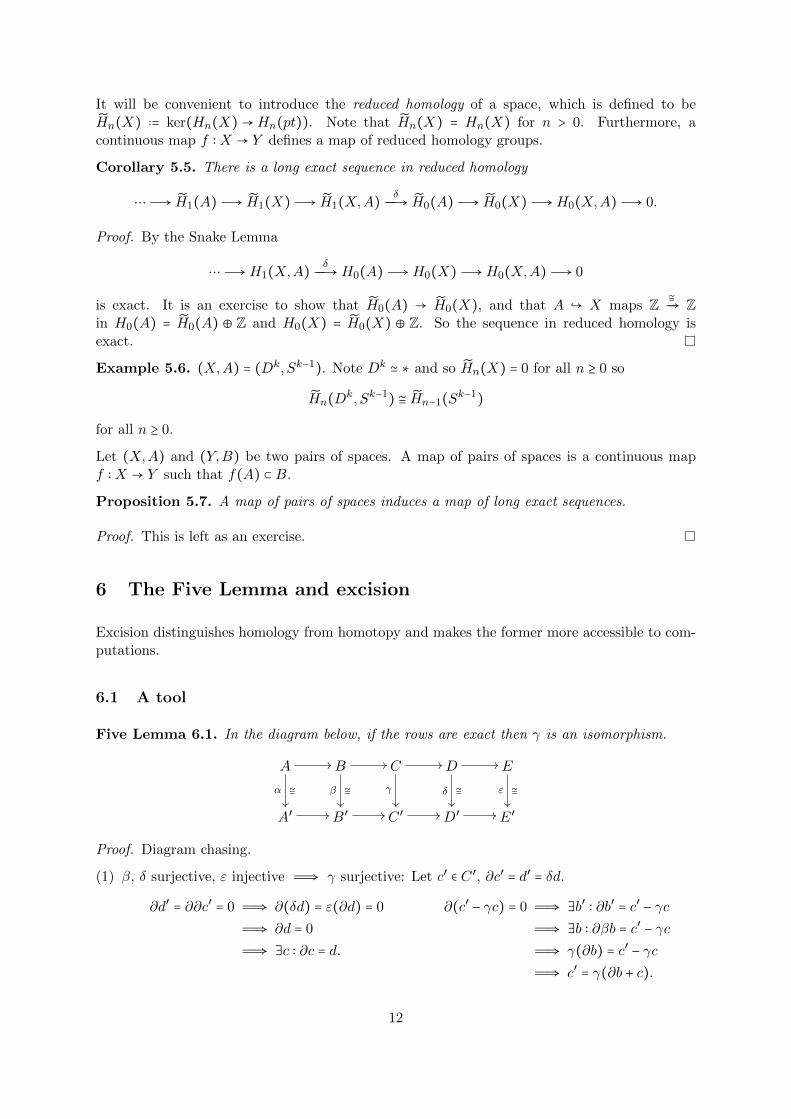
Five Lemma 6.1. In the diagram below, if the rows are exact then γ is an isomorphism.

A //

≅α

��

B //

≅β��

C //

γ

��

D //

≅δ��

E

≅ε

��

A′ // B′ // C ′ // D′ // E′

Proof. Diagram chasing.

(1) β, δ surjective, ε injective Ô⇒ γ surjective: Let c′ ∈ C ′, ∂c′ = d′ = δd.

∂d′ = ∂∂c′ = 0 Ô⇒ ∂(δd) = ε(∂d) = 0

Ô⇒ ∂d = 0

Ô⇒ ∃c ∶ ∂c = d.

∂(c′ − γc) = 0 Ô⇒ ∃b′ ∶ ∂b′ = c′ − γcÔ⇒ ∃b ∶ ∂βb = c′ − γcÔ⇒ γ(∂b) = c′ − γcÔ⇒ c′ = γ(∂b + c).

12

(2) β, δ injective, α surjective Ô⇒ γ injective: similarly.

Example 6.2. Assume 0 // Gα // H

β// K //

γii i_U 0 is split exact with β ○ γ = id. Ap-

plying the Five Lemma to

0 // G // H // K // 0

0 // G // G⊕K //

α⋅γOO

K // 0

gives H ≃ G⊕K.

6.2 Excision

Definition 6.3. Let A ⊂ X be a subspace. A map r ∶ X → X is a retract onto A if r(X) = Aand r∣A = idA (so r2 = r). If r is a homotopy equivalence (rel A) then r is a deformation retract.

A pair (X,A) is called good if A is a non-empty, closed subset of X suchthat it is a deformation retract of some neighbourhood V of A in X. A

X

V

Define the quotient X/A as the quotient under the equivalence relation x ∼ y iff (x ∈ A andy ∈ A) or (x = y).

Example 6.4. X = S1 ∨ S1 ⊇ A = S1 V = X/A ≃ with [A] =

Example 6.5. X =Dk ⊇ A = Sk−1 V = X/A ≃ Sk with [Sk−1] = a point.

Theorem 6.6 (Excision and relative homology as the homology of a space). Let A ⊂ V ⊂X besubspaces of X such that A ⊂ V . Then the map of pairs (X ∖A,V ∖A) → (X,V ) induces an

isomorphism Hn(X ∖A,V ∖A) ≅Ð→Hn(X,V ) for all n ≥ 0.

Corollary 6.7. For a good pair (X,A), the quotient map (X,A) → (X/A,∗) induces an iso-

morphism Hn(X,A) ≅Ð→Hn(X/A,∗) = Hn(X/A) for all n ≥ 0.

Proof of corollary. As (X,A) is good there exists V ⊃ A such that A ↪ V is a homotopyequivalence. Consider the following commutative diagram.

Hn(X,A) ≅ //

q

��

Hn(X,V )

q

��

Hn(X ∖A,V ∖A)≅oo

q

Hn(X/A,A/A) ≅ // Hn(X/A,V /A) Hn(X/A ∖A/A,V /A ∖A/A)≅oo

Using Proposition 5.7 and the Five Lemma one shows that the left horizontal arrows are isomor-

phisms since A≃Ð→ V and A/A ≃Ð→ V /A are homotopy equivalences. The right horizontal arrows

are isomorphisms by excision and the right vertical arrow is the identity as X/A∖A/A =X ∖A.The diagram commutes and therefore also the other two vertical arrows are isomorphisms.

Example 6.8. (Dk, Sk−1) is good Ô⇒ Hn(Dk, Sk−1) ≅ Hn(Dk/Sk−1) ≅ Hn(Sk).

13

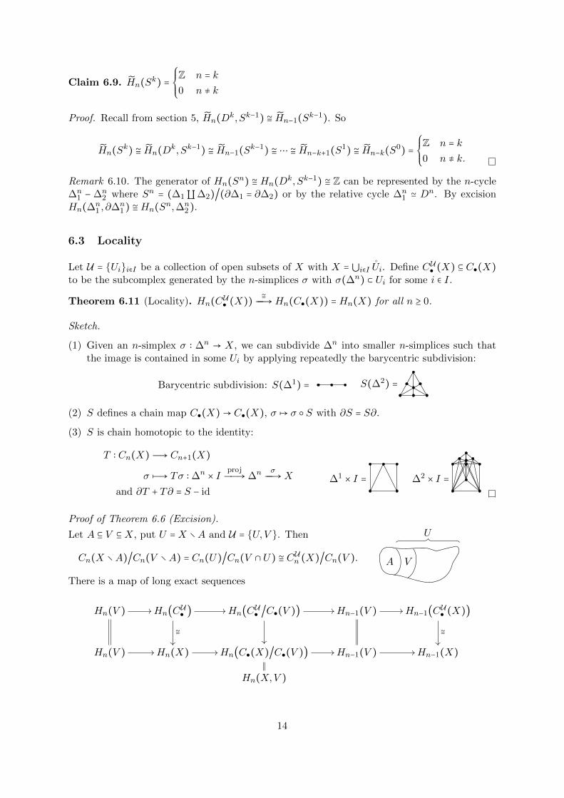
Claim 6.9. Hn(Sk) =⎧⎪⎪⎨⎪⎪⎩

Z n = k0 n ≠ k

Proof. Recall from section 5, Hn(Dk, Sk−1) ≅ Hn−1(Sk−1). So

Hn(Sk) ≅ Hn(Dk, Sk−1) ≅ Hn−1(Sk−1) ≅ ⋯ ≅ Hn−k+1(S1) ≅ Hn−k(S0) =⎧⎪⎪⎨⎪⎪⎩

Z n = k0 n ≠ k.

Remark 6.10. The generator of Hn(Sn) ≅ Hn(Dk, Sk−1) ≅ Z can be represented by the n-cycle∆n

1 − ∆n2 where Sn = (∆1∐∆2)/(∂∆1 = ∂∆2) or by the relative cycle ∆n

1 ≃ Dn. By excisionHn(∆n

1 , ∂∆n1) ≅Hn(Sn,∆n

2).

6.3 Locality

Let U = {Ui}i∈I be a collection of open subsets of X with X = ⋃i∈I Ui. Define CU● (X) ⊆ C●(X)to be the subcomplex generated by the n-simplices σ with σ(∆n) ⊂ Ui for some i ∈ I.

Theorem 6.11 (Locality). Hn(CU● (X)) ≅ÐÐ→Hn(C●(X)) =Hn(X) for all n ≥ 0.

Sketch.

(1) Given an n-simplex σ ∶ ∆n → X, we can subdivide ∆n into smaller n-simplices such thatthe image is contained in some Ui by applying repeatedly the barycentric subdivision:

Barycentric subdivision: S(∆1) = S(∆2) =

(2) S defines a chain map C●(X)→ C●(X), σ ↦ σ ○ S with ∂S = S∂.

(3) S is chain homotopic to the identity:

T ∶ Cn(X)Ð→ Cn+1(X)

σ z→ Tσ ∶ ∆n × IprojÐÐ→∆n σÐÐ→X

and ∂T + T∂ = S − id∆1 × I = ∆2 × I =

Proof of Theorem 6.6 (Excision).

Let A ⊆ V ⊆X, put U =X ∖A and U = {U,V }. Then

Cn(X ∖A)/Cn(V ∖A) = Cn(U)/Cn(V ∩U) ≅ CUn (X)/Cn(V ).

There is a map of long exact sequences

A V

U

Hn(V ) // Hn(CU● ) //

≅��

Hn(CU● /C●(V )) //

��

Hn−1(V ) // Hn−1(CU● (X))

≅��

Hn(V ) // Hn(X) // Hn(C●(X)/C●(V )) // Hn−1(V ) // Hn−1(X)

Hn(X,V )

14

So by the Five Lemma:

Hn(X ∖A,V ∖A) ≅Hn(CU● /C●(V )) ≅Hn(X,V ).

6.4 Mayer-Vietoris sequence

‘Divide and conquer: Part II’

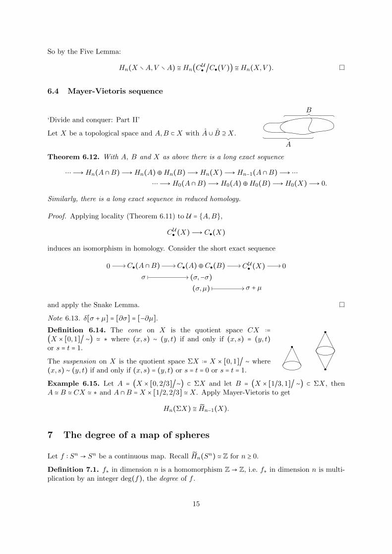
Let X be a topological space and A,B ⊂X with A ∪ B ⊇X.

B

A

Theorem 6.12. With A, B and X as above there is a long exact sequence

⋯Ð→Hn(A ∩B)Ð→Hn(A)⊕Hn(B)Ð→Hn(X)Ð→Hn−1(A ∩B)Ð→ ⋯⋯Ð→H0(A ∩B)Ð→H0(A)⊕H0(B)Ð→H0(X)Ð→ 0.

Similarly, there is a long exact sequence in reduced homology.

Proof. Applying locality (Theorem 6.11) to U = {A,B},

CU● (X)Ð→ C●(X)

induces an isomorphism in homology. Consider the short exact sequence

0 // C●(A ∩B) // C●(A)⊕C●(B) // CU● (X) // 0

σ � // (σ,−σ)(σ,µ) � // σ + µ

and apply the Snake Lemma.

Note 6.13. δ[σ + µ] = [∂σ] = [−∂µ].Definition 6.14. The cone on X is the quotient space CX ..=(X × [0,1]/ ∼) ≃ ∗ where (x, s) ∼ (y, t) if and only if (x, s) = (y, t)or s = t = 1.

The suspension on X is the quotient space ΣX ..= X × [0,1]/ ∼ where(x, s) ∼ (y, t) if and only if (x, s) = (y, t) or s = t = 0 or s = t = 1.

Example 6.15. Let A = (X × [0,2/3]/∼) ⊂ ΣX and let B = (X × [1/3,1]/ ∼) ⊂ ΣX, thenA ≃ B ≃ CX ≃ ∗ and A ∩B =X × [1/2,2/3] ≃X. Apply Mayer-Vietoris to get

Hn(ΣX) ≅ Hn−1(X).

7 The degree of a map of spheres

Let f ∶ Sn → Sn be a continuous map. Recall Hn(Sn) ≃ Z for n ≥ 0.

Definition 7.1. f∗ in dimension n is a homomorphism Z → Z, i.e. f∗ in dimension n is multi-plication by an integer deg(f), the degree of f .

15

Note 7.2. (i) deg(idSn) = 1 as (idSn)∗ = idHn(ii) deg(f ○ g) = deg(f) ⋅ deg(g) as (f ○ g)∗ = f∗ ○ g∗

(iii) f ≃ g Ô⇒ deg(f) = deg(g) as f∗ = g∗(iv) f ≃ ∗ Ô⇒ deg(f) = 0 as f∗ = 0.

Example 7.3.

(1) f is induced by the reflection in Rni × {0} ⊂ Rn+1, thendeg(f) = −1:Hn(Sn) = ⟨∆1 − ∆2⟩, f interchanges ∆1 and ∆2. Sof∗(∆1 −∆2) = (∆2 −∆1) = −(∆1 −∆2).

01

2

(2) f is the antipodal map Sn → Sn, x↦ −x, then deg(f) = (−1)n+1:

f is induced by −I ∶ Rn+1 → Rn+1, −I = (−1 0 ⋯ 00 1 0⋮ ⋱ ⋮0 0 ⋯ 1

)(1 0 ⋯ 00 −1 0⋮ ⋱ ⋮0 0 ⋯ 1

)⋯(1 ⋯ 0 0⋮ ⋱ ⋮0 1 00 ⋯ 0 −1

).

Each of the n+ 1 matrices on the right hand side is a reflection homotopic to the one in (1)hence, using (ii) and (iii), deg(f) = (−1)n+1.

Application 7.4. A continuous function v ∶ Sn → Rn+1 definesa tangent vector field on Sn if v(x) ⊥ x for all x ∈ Sn. Sn has acontinuous nowhere zero tangent vector field if and only if n is odd.

Proof. Suppose v ∶ Sn → Rn+1 is continuous with v(x) ⊥ x for all x. Suppose further v(x) ≠ 0

for all x. Consider F ∶ Sn × [0,1]→ Sn given by F (x, t) = (cosπt)x + (sinπt) v(x)∣v(x)∣ .

Note F (x,0) = x and F (x,1) = −x. Hence F defines a homotopyfrom the identity map to the antipodal map. Hence they must havethe same degree (by (iii)) and 1 = (−1)n+1. So n must be odd.

Conversely, if n is odd, define

v ∶ Sn Ð→ Rn+1

(x1, . . . , x2k)z→ (−x2, x1, . . . ,−x2k, x2k−1).

x−x

v(x)∣v(x)∣

Corollary 7.5 (Hairyi ball theorem). You cannot comb a hairy ball (S2).

Definition 7.6. Let f(x) = y and U ∋ x, V ∋ y be open neighbourhoods of x and y respectivelysuch that

f ∶ (U,U ∖ x)Ð→ (V,V ∖ y) (∗)

i.e. the only point in U mapping to y is x.

From the relative long exact sequence and excision we have

Z ≅ Hn(Sn) ≅Hn(Sn, Sn ∖ x) ≅Hn(U,U ∖ x)(f ∣x)∗ÐÐÐ→Hn(V,V ∖ y) ≅ Hn(Sn) ≅ Z.

Then (f ∣x)∗ is multiplication by an integer deg(f ∣x), the local degree of f at x.

16

Proposition 7.7. Assume f−1(y) = {x1, . . . , xk} and for eachi = 1, . . . , k there exist disjoint open sets Ui ∋ xi each satisfyingcondition (∗). Then

deg(f) =k

∑i=1

deg(f ∣xi).

If f−1(y) = ∅ then deg(f) = 0.

x1x2

y

Proof. The proposition follows from the following commutative diagram:

Hn(Sn)f∗

//

q

��

Hn(Sn)

≅��

Hn(Sn, Sn ∖ {x1, . . . , xk})f∗

//

≅��

Hn(V,V ∖ y)

⊕ki=1Hn(Ui, Ui ∖ xi)

∑i(f ∣xi)∗

44jjjjjjjjjjjjjjj

Example 7.8. Let f ∶ S2 = C ∪ {∞} → S2 be define by f(z) = zn. Let y = 1, thenf−1(y) = {e2πki/n ∶ k = 1, . . . n}. Since f is orientation preserving and is a homeomorphism neareach root of unity, deg(f ∣e2πki/n) = 1. Hence deg(f) = n.

• For p an arbitrary polynomial of degree n, p ≃ f (via a homotopy that moves all zeros to0). Hence deg(p) = n.

• deg(f ∣0) = n.

8 Cellular homology

Definition 8.1 (CW-complex). Inductive construction:

(1) Start with X0, a disjoint set (X−1 = ∅).

(2) Let Dnα be an n-disk and φα ∶ ∂Dn

α ≃ Sn−1 → Xn−1 be a continuous map. For a collection{Dn

α, φα} construct Xn from Xn−1 by Xn ..=Xn−1∐αDnα/x ∼ φα(x) for all x ∈ ∂Dn

α.

(3) X = ⋃nXn is given the weak topology (A ⊂ X is open if and only if A ∩Xn is open for alln).

Dnα = enα is called an n-cell. Each cell has a characteristic map enα ↪X.

Example 8.2.

X0 = ptX1 =X2 = ⋃

φ

D2 φ ∶ S1 → S1 of degree 3

17

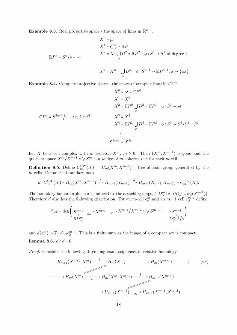
Example 8.3. Real projective space - the space of lines in Rn+1.

RPn = Sn/v ∼ −v

X0 = ptX1 = = RP 1

X2 =X1⋃φ

D2 = RP 2 φ ∶ S1 → S1 of degree 2

⋮Xn =Xn−1⋃

φ

Dn φ ∶ Sn−1 → RPn−1, x↦ {±x}

Example 8.4. Complex projective space - the space of complex lines in Cn+1.

CPn = S2n+1/v ∼ λv, λ ∈ S1

X0 = pt = CP 0

X1 =X0

X2 = CP 0⋃φ

D2 = CP 1 φ ∶ S1 → pt

X3 =X2

X4 = CP 1⋃φ

D4 = CP 2 φ ∶ S3 → S3/S1 ≃ S2

⋮X2k+1 =X2k

Let X be a cell complex with m skeleton Xm, m ≥ 0. Then (Xm,Xm−1) is good and thequotient space Xm/Xm−1 ≃ ⋁Sm is a wedge of m-spheres, one for each m-cell.

Definition 8.5. Define CCWm (X) ..= Hm(Xm,Xm−1) = free abelian group generated by the

m-cells. Define the boundary map

d ∶ CCWm (X) =Hm(Xm,Xm−1) δÐ→Hm−1(Xm−1)qÐ→Hm−1(Xm−1,Xm−2) = CCWm−1(X).

The boundary homomorphism δ is induced by the attaching maps, δ[Dmα ] = [∂Dm

α ≡ φα(Sm−1)].Therefore d also has the following description. For an m-cell emα and an m − 1 cell em−1

β define

dαβ ..= deg( Sm−1φα

// Xm−1q

// Xm−1/Xm−2 ≃ ⋁Sm−1 // Sm−1

∂Dmα Dm−1

β /∂

)

and d(emα ) ..= ∑β dαβem−1β . This is a finite sum as the image of a compact set is compact.

Lemma 8.6. d ○ d = 0

Proof. Consider the following three long exact sequences in relative homology.

Hm+1(Xm+1,Xm) δ // Hm(Xm)

jjjjjjjjjjjjj

jjjjjjjjjjjjj// Hm(Xm+1) //

// Hm(Xm) q∗// Hm(Xm,Xm−1) δ // Hm−1(Xm−1)

jjjjjjjjjjjjj

jjjjjjjjjjjjj

// Hm−1(Xm−1) q∗// Hm−1(Xm−1,Xm−2)

(∗∗)

18

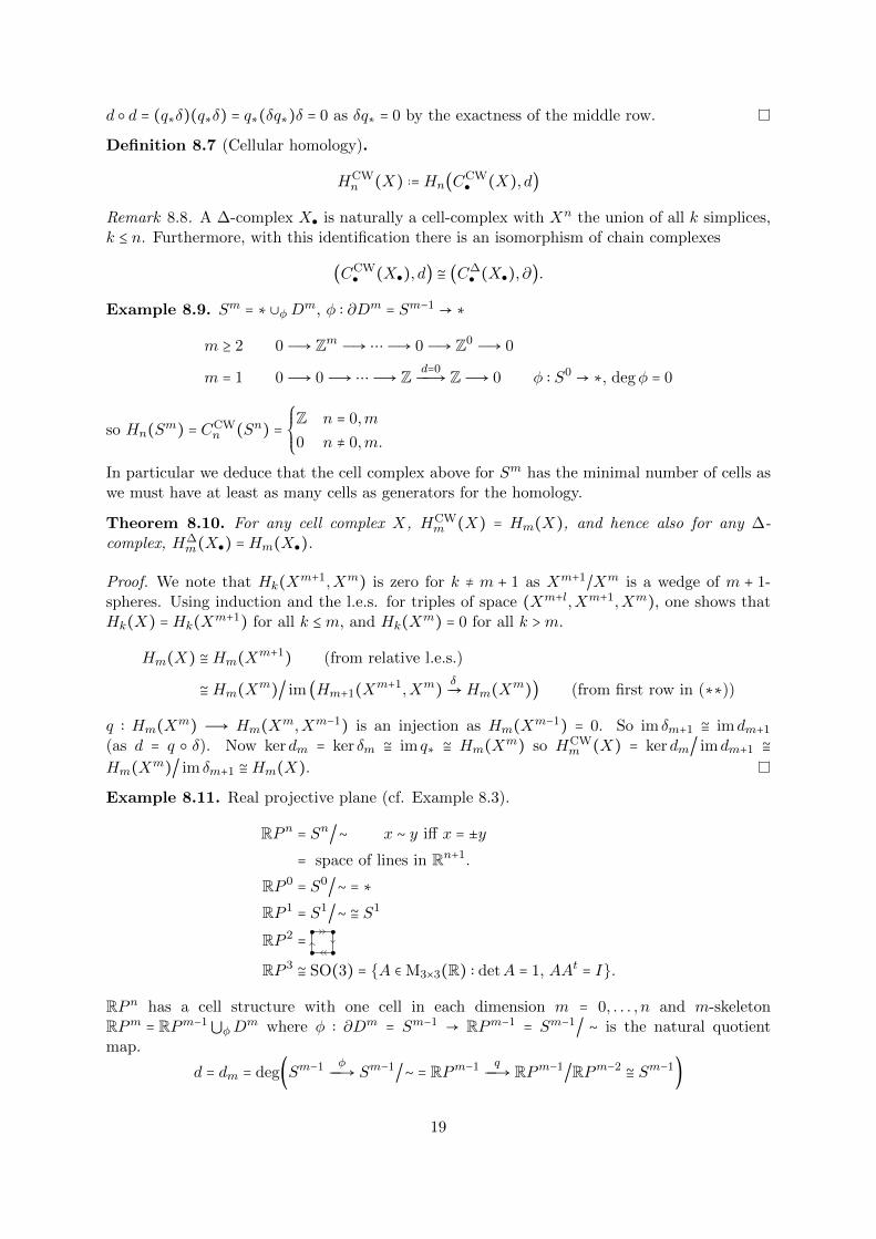
d ○ d = (q∗δ)(q∗δ) = q∗(δq∗)δ = 0 as δq∗ = 0 by the exactness of the middle row.

Definition 8.7 (Cellular homology).

HCWn (X) ..=Hn(CCW

● (X), d)

Remark 8.8. A ∆-complex X● is naturally a cell-complex with Xn the union of all k simplices,k ≤ n. Furthermore, with this identification there is an isomorphism of chain complexes

(CCW● (X●), d) ≅ (C∆

● (X●), ∂).

Example 8.9. Sm = ∗ ∪φDm, φ ∶ ∂Dm = Sm−1 → ∗

m ≥ 2 0Ð→ Zm Ð→ ⋯Ð→ 0Ð→ Z0 Ð→ 0

m = 1 0Ð→ 0Ð→ ⋯Ð→ Z d=0ÐÐ→ ZÐ→ 0 φ ∶ S0 → ∗, degφ = 0

so Hn(Sm) = CCWn (Sn) =

⎧⎪⎪⎨⎪⎪⎩

Z n = 0,m

0 n ≠ 0,m.

In particular we deduce that the cell complex above for Sm has the minimal number of cells aswe must have at least as many cells as generators for the homology.

Theorem 8.10. For any cell complex X, HCWm (X) = Hm(X), and hence also for any ∆-

complex, H∆m(X●) =Hm(X●).

Proof. We note that Hk(Xm+1,Xm) is zero for k ≠ m + 1 as Xm+1/Xm is a wedge of m + 1-spheres. Using induction and the l.e.s. for triples of space (Xm+l,Xm+1,Xm), one shows thatHk(X) =Hk(Xm+1) for all k ≤m, and Hk(Xm) = 0 for all k >m.

Hm(X) ≅Hm(Xm+1) (from relative l.e.s.)

≅Hm(Xm)/ im (Hm+1(Xm+1,Xm) δÐ→Hm(Xm)) (from first row in (∗∗))

q ∶ Hm(Xm) Ð→ Hm(Xm,Xm−1) is an injection as Hm(Xm−1) = 0. So im δm+1 ≅ imdm+1

(as d = q ○ δ). Now kerdm = ker δm ≅ im q∗ ≅ Hm(Xm) so HCWm (X) = kerdm/ imdm+1 ≅

Hm(Xm)/ im δm+1 ≅Hm(X).

Example 8.11. Real projective plane (cf. Example 8.3).

RPn = Sn/∼ x ∼ y iff x = ±y= space of lines in Rn+1.

RP 0 = S0/∼ = ∗RP 1 = S1/∼ ≅ S1

RP 2 =

RP 3 ≅ SO(3) = {A ∈ M3×3(R) ∶ detA = 1, AAt = I}.

RPn has a cell structure with one cell in each dimension m = 0, . . . , n and m-skeletonRPm = RPm−1⋃φDm where φ ∶ ∂Dm = Sm−1 → RPm−1 = Sm−1/ ∼ is the natural quotientmap.

d = dm = deg(Sm−1 φÐÐ→ Sm−1/∼ = RPm−1 q

ÐÐ→ RPm−1/RPm−2 ≅ Sm−1)

19

q ○φ∣∆+ , q ○φ∣∆− are homeomorphisms onto their images which are related to each other via theantipodal map.

Ô⇒ d = dm = deg(q ○ φ) = deg(id) + deg(antipodal map)= 1 + (−1)m

Ô⇒ CCW● (RPn) =

⎧⎪⎪⎨⎪⎪⎩

0Ð→ Z 0ÐÐ→ Z 2ÐÐ→ ⋯ 2ÐÐ→ Z 0ÐÐ→ Z 0ÐÐ→ 0 m odd

0Ð→ 00ÐÐ→ Z 2ÐÐ→ ⋯ 2ÐÐ→ Z 0ÐÐ→ Z 0ÐÐ→ 0 m even

Ô⇒ Hm(RPn) =

⎧⎪⎪⎪⎪⎪⎪⎪⎨⎪⎪⎪⎪⎪⎪⎪⎩

Z m = 0

Z/2 m odd and m < nZ m = n odd

0 otherwise.

9 Cohomology and the Universal Coefficient Theorem

9.1 Cohomology

Definition 9.1. Let (C●, ∂●) be a chain complex of free Z-modules (or F-vector spaces). Define

• n-cochains: Cn ..= Hom(Cn,Z), group of group homomorphisms (or the dual vector space)

• coboundary map: ∂n ∶ Cn → Cn+1, φ↦ φ ○ ∂

• n-cocycle: Zn = ker(∂n)

• n-coboundary: Bn = im(∂n−1)

• n-th cohomology group: Hn(C,∂) ..=Hn(C●, ∂●) = Zn/Bn.

We note that Hom(Zn,Z) ≃ Zn, and if a matrix A represents an element in Hom(Zn,Zm thenthe dual map is represented by its transpose.

Example 9.2. The cellular chain complex for RP 3 is

0Ð→ Z 0ÐÐ→ Z 2ÐÐ→ Z 0ÐÐ→ ZÐ→ 0.

As Hom(Z,Z) ≅ Z the dual complex is

0←Ð Z 0←ÐÐ Z 2←ÐÐ Z 0←ÐÐ Z←Ð 0.

Hence

Hn(RP 3) =

⎧⎪⎪⎪⎪⎪⎪⎪⎪⎪⎪⎨⎪⎪⎪⎪⎪⎪⎪⎪⎪⎪⎩

Z n = 0

0 n = 1

Z/2 n = 2

Z n = 3

0 n > 3.

Induced Homomorphism. f ∶X Ð→ Y induces

f♯ ∶ Cn(X)Ð→ Cn(Y ) and hence

f ♯ ∶ Cn(Y )Ð→ Cn(X), φz→ φ ○ f♯f∗ ∶Hn(Y )Ð→Hn(X)

20

Lemma 9.3. If f●, g● ∶ (C●, ∂●) → (C●, ∂●) are chain homotopic then so are f●, g● ∶ (C●, ∂●) →(C●, ∂●) and f● = g● ∶Hn(C●, ∂●)→Hn(C●, ∂●).

Proof. If f● − g● = ∂●h● + h●∂● then f● − g● = h●∂● + ∂●h●.

Homotopy Invariance. If f ≃ g ∶X → Y then f∗ = g∗ ∶Hn(Y )→Hn(X).

Lemma 9.4. If 0 → A●i●Ð→ C●

j●Ð→ B● → 0 is an exact sequence of free chain complexes then so

is 0← A● i●←Ð C● j●←Ð B● ← 0.

Proof. Consider 0 → An → Cn → Bn → 0. As Bn is free there is a splitting s ∶ Bn → Cn and

Cni⊕sÐÐ→≅ An ⊕Bn. Hence

Cn = Hom(Cn,Z) ≅ Hom(An,Z)⊕Hom(Bn,Z) ≅ An ⊕Bn

φ↦ ((φ ○ i), (φ ○ s))

and ker i∗ = im j∗.

Excision. If Z ⊂ A ⊂X then Hn(X,A) i∗Ð→≅ Hn(X ∖Z,A ∖Z).

Long Exact Relative Cohomology Sequence. For any (X,A) there is a long exact se-quence

⋯←ÐH1(X,A) δ1←ÐÐH0(A)←ÐH0(X)←ÐH0(X,A)←Ð 0.

Mayer-Vietoris. For A ∪ B =X there is a long exact sequence

⋯←ÐH1(X) δ1←ÐÐH0(A ∩B)←ÐH0(A)⊕H0(B)←ÐH0(X)←Ð 0.

9.2 Universal Coefficient Theorem

Relating H∗ to H∗.

Let (C●, ∂●) be a chain complex of free abelian groups (or vector spaces). Then Cn, Bn and Znare all free. Hence the short exact sequence

0Ð→ Zn Ð→ Cn∂nÐÐ→ Bn−1 Ð→ 0 (9.1)

gives rise to a short exact sequence of dual chain complexes

0 Znoo Cnoo Bn−1∂noo 0oo

0 Zn−1

∂n=0

OO

oo Cn−1

∂n

OO

oo Bn−2

∂n−1=0

OO

∂n−1oo 0oo

21

and a long exact sequence in homology

⋯←Ð Bn ←Ð Zn ←ÐHn(C●)←Ð Bn−1 ←Ð Zn−1 ←Ð ⋯

so there are short exact sequences

0 ker inoo66S _ kHn(C●)oo coker inoo 0oo (∗)

and ker in = {φ ∈ Zn ∶ φ∣Bn ≅ 0} = {φ ∈ (Zn/Bn)∗} = (Hn(C●))∗.

If we are working over a field and assuming that Hn(C●) is finite dimensional, coker in = 0 asevery f ∈ Bn−1 can be extended to f ∈ Zn−1.

Theorem 9.5. If (C●, ∂●) is a chain complex of vector spaces with finite dimensional cohomol-ogy, then Hn(C●) = (Hn(C●))∗.

Corollary 9.6. For any space X of finite type and any field F, Hn(X;F) ≅ (Hn(X;F))∗.

Let (C●, ∂●) now be a chain complex of free, finitely generated abelian groups. Then

in−1 =

⎛⎜⎜⎜⎜⎜⎝

d1⋱dk

1⋱

10 ⋯ ⋯ ⋯ ⋯ 0⋮ ⋮0 ⋯ ⋯ ⋯ ⋯ 0

⎞⎟⎟⎟⎟⎟⎠

∶ Bn−1 Ð→ Zn−1

and hence Hn−1 = Zl ⊕ (Z/d1Z)⊕⋯⊕ (Z/dkZ). Also

in−1 = (d1

⋱1

0 ⋯ 0

)t

=⎛⎜⎜⎝

d1 0 ⋯ 0⋱ ⋮ ⋮dk ⋮ ⋮

1 ⋮ ⋮⋱ ⋮ ⋮

1 0 ⋯ 0

⎞⎟⎟⎠

andcoker in−1 = Bn−1/ im in−1 ≅ (Z/d1Z)⊕⋯⊕ (Z/dkZ) ≅ Tor(Hn−1)

Theorem 9.7. If (C●, ∂●) is a chain complex of finitely generated free abelian groups then

Hn(C●) ≅ (Hn(C●))∗ ⊕Tor(Hn−1(C●))

Corollary 9.8. For a cell complex of finite type, i.e. a complex with finitely many cells in eachdimension,

Hn(X) ≅ (Hn(X)/Tor(Hn(X)))⊕Tor(Hn−1(X)).

Furthermore, (Hn(C●))∗ is free and so the short exact sequence (∗) splits.

Remark 9.9. A map of chain complexes C● → C● induces a map of exact sequences in (∗).However, the splitting in Theorem 9.7 does not correspond, i.e. the splitting may not be natural.

Example 9.10.

H0(RP 3) = ZH0(RP 3) = Z

H1(RP 3) = Z/2ZH1(RP 3) = 0

H2(RP 3) = 0

H2(RP 3) = Z/2ZH3(RP 3) = ZH3(RP 3) = Z

22

10 The Kunneth Theorem and products

10.1 Algebraic Kunneth formula

Definition 10.1. If A and B are abelian group (or F vector spaces) define their tensor productA⊗B to be the abelian group generated by {a⊗ b}a∈A,b∈B subject to the relation

(1) a⊗ (b + b′) = (a⊗ b) + (a⊗ b′) for a ∈ A and b, b′ ∈ B

(2) (a + a′)⊗ b = (a⊗ b) + (a′ ⊗ b) for a, a′ ∈ A and b ∈ B

(3) na⊗ b = a⊗ nb for a ∈ A, b ∈ B and n ∈ Z (or n ∈ F).

Example 10.2.

(i) Z/nZ⊗Z ≅ Z/nZ as 1⊗ k = k ⊗ 1

(ii) Z/2Z⊗Z/4Z ≅ Z/2Z

(iii) Z/2Z⊗Z/3Z ≅ 0

(iv) Zn ⊗Zm ≅ Znm

If C● and C● are two chain complexes of abelian groups (or F vector spaces) then define theirtensor product as

(C● ⊗ C●)n..=

n

∑k=0

Ck ⊗ Cn−k and ∂(c⊗ c) ..= ∂c⊗ c + (−1)deg cc⊗ ∂c.

Check:

• ∂ ○ ∂ = 0

• Zk ⊗Zn−k ⊆ Zn(C● ⊗ C●)

• Zk ⊗Bn−k, Bk ⊗Zn−k ⊆ Bn(C● ⊗ C●)

Proposition 10.3. If C● ⊗ C● is a chain complex and there are natural maps

Hk(C●)⊗Hn−k(C●)Ð→Hn(C● ⊗ C●).

Theorem 10.4. (Algebraic Kunneth formula) Assume Ck and Hk(C●) are finitely generatedand free. Then

n

⊕k=0

Hk(C●)⊗Hn−k(C●)≅ÐÐ→Hn(C● ⊗ C●).

10.2 The cup product

Let X be a space and let (C●(X), ∂●) be its singular (or simplicial) cochain complex. Forϕ ∈ Ck(X) = Hom(Ck(X),Z) and ψ ∈ C l(X), the cup product ϕ ⌣ ψ ∈ Ck+l(X) is the cochainthat maps σ ∶ ∆k+l →X to

(ϕ ⌣ ψ)(σ) = ϕ(σ∣[v0,...,vk]) ⋅ ψ(σ∣[vk,...,vk+l]).

Lemma 10.5. ∂●(ϕ ⌣ ψ) = ∂●ϕ ⌣ ψ + (−1)kϕ ⌣ ∂●ψ.

23

Proof. Let σ ∶ ∆k+l+1 →X be a singular simplex. Then

∂●(ϕ ⌣ ψ)(σ) = (ϕ ⌣ ψ)(∂σ)

= (ϕ ⌣ ψ)(k+l+1

∑i=0

(−1)iσ∣[v0,...,vi,...,vk+l+1])

=k

∑i=0

(−1)iϕ(σ∣[v0,...,vi,...,vk+1]) ⋅ ψ(σ∣[vk+1,...,vk+l+1])

+k+l+1

∑i=k+1

(−1)iϕ(σ∣[v0,...,vk]) ⋅ ψ(σ∣[vk,...,vi,...,vk+l+1])

= (∂●ϕ ⌣ ψ)(σ) + (−1)k(ϕ ⌣ ∂●ψ)(σ)

Corollary 10.6. The cup product induces an associative and distributive multiplication in co-homology

Hk(X) ×H l(X)Ð→Hk+l(X).

Note 10.7. The cup product is graded commutative in the sense that

[ϕ] ⌣ [ψ] = (−1)kl[ψ] ⌣ [φ].

Proof. Well-defined:

ϕ ∈ Zk, ψ ∈ Z l Ô⇒ ∂●(ϕ ⌣ ψ) ∈ Zk+l by the lemma

ϕ = ϕ + β, β ∈ Bk Ô⇒ ϕ ⌣ ψ = ϕ ⌣ ψ + β ⌣ ψ

but β = ∂●γ, so β ⌣ ψ = ∂●γ ⌣ ψ = ∂●(γ ⌣ ψ)

hence [ϕ ⌣ ψ] = [ϕ ⌣ ψ].

Unit:Let ε ≡ 1 ∈ C0(X) be the constant map to 1. For a 1-simplex σ

(∂●ε)(σ) = ε(σ∣[v1]) − ε(σ∣[v0])

hence [ε] ∈H0(X) is the unit in cohomology and

H0(X) ×Hn(X)--ZZZZZ (m[ε], ϕ) � ,,XXXXXHn(X) mφ

Hn(X) ×H0(X)11ddddd

(ϕ,m[ε])& 22fffff

Proposition 10.8. If f ∶ X → Y then f ♯(ϕ ⌣ ψ) = f ♯(ϕ) ⌣ f ♯(ψ), i.e. f ♯ commutes with cupproducts. Hence f∗ ∶H∗(Y )→H∗(X) is a map of rings.

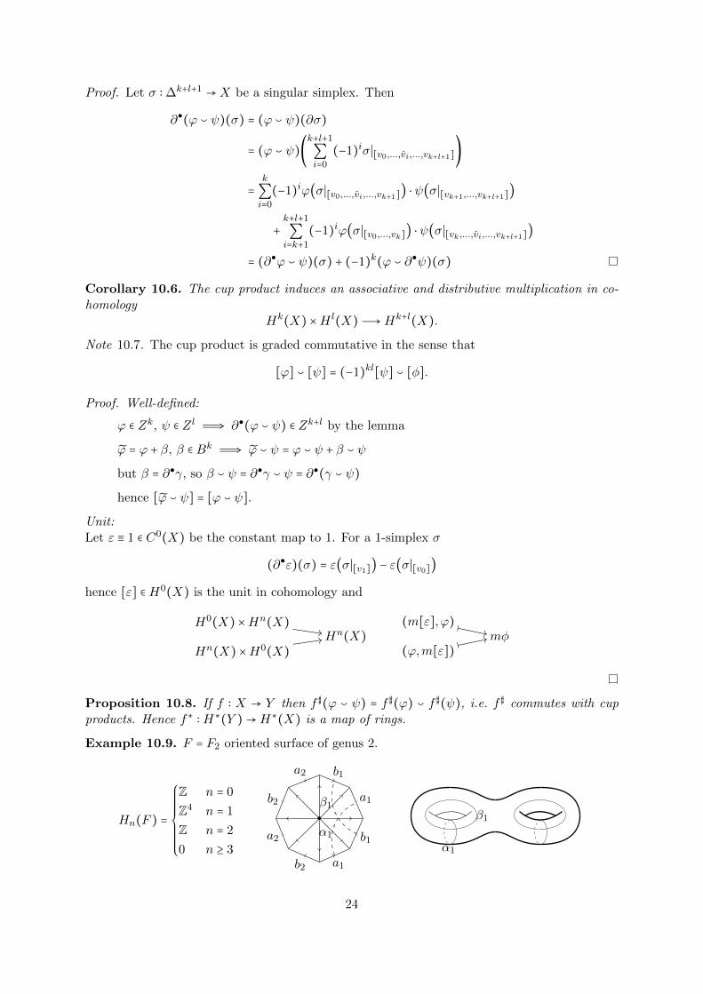
Example 10.9. F = F2 oriented surface of genus 2.

Hn(F ) =

⎧⎪⎪⎪⎪⎪⎪⎪⎨⎪⎪⎪⎪⎪⎪⎪⎩

Z n = 0

Z4 n = 1

Z n = 2

0 n ≥ 3

a1

b1

a1

b1

a2

b2

a2

b2

α1

β1

α1

β1

24

So Hn(F ) ≅Hn(F ) by the Universal Coefficient Theorem. For dimensional reasons, all productsare either multiplication by a constant (above) or zero, with the exception of

H1(F ) ×H1(F )Ð→H2(F )

H1(F ) = (H1(F ))∗ = Z4 is generated by a∗1 , b∗1 , a

∗2 , b

∗2 . H2(F ) = (H2(F ))∗ is generated by c∗.

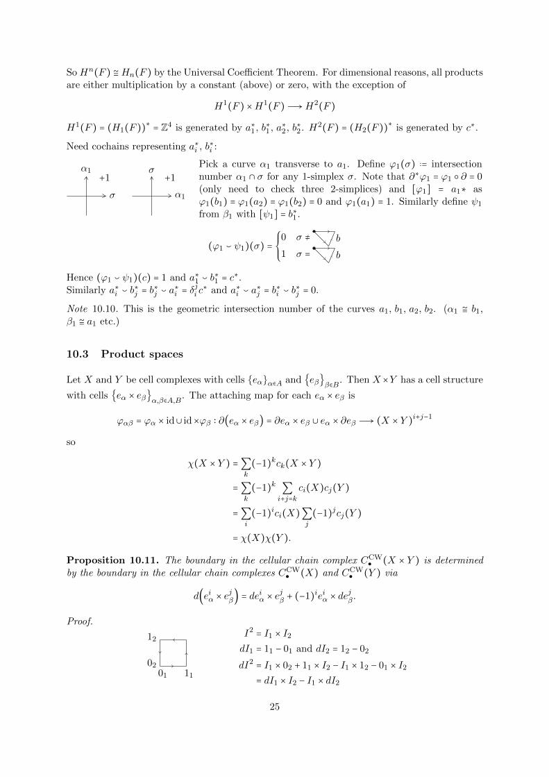
Need cochains representing a∗i , b∗i :

α1

σ

+1σ

α1

+1

Pick a curve α1 transverse to a1. Define ϕ1(σ) ..= intersectionnumber α1 ∩ σ for any 1-simplex σ. Note that ∂∗ϕ1 = ϕ1 ○ ∂ = 0(only need to check three 2-simplices) and [ϕ1] = a1∗ asϕ1(b1) = ϕ1(a2) = ϕ1(b2) = 0 and ϕ1(a1) = 1. Similarly define ψ1

from β1 with [ψ1] = b∗1 .

(ϕ1 ⌣ ψ1)(σ) =⎧⎪⎪⎨⎪⎪⎩

0 σ ≠ b

1 σ = b

Hence (ϕ1 ⌣ ψ1)(c) = 1 and a∗1 ⌣ b∗1 = c∗.Similarly a∗i ⌣ b∗j = b∗j ⌣ a∗i = δ

ji c∗ and a∗i ⌣ a∗j = b∗i ⌣ b∗j = 0.

Note 10.10. This is the geometric intersection number of the curves a1, b1, a2, b2. (α1 ≅ b1,β1 ≅ a1 etc.)

10.3 Product spaces

Let X and Y be cell complexes with cells {eα}α∈A and {eβ}β∈B. Then X ×Y has a cell structure

with cells {eα × eβ}α,β∈A,B. The attaching map for each eα × eβ is

ϕαβ = ϕα × id∪ id×ϕβ ∶ ∂(eα × eβ) = ∂eα × eβ ∪ eα × ∂eβ Ð→ (X × Y )i+j−1

so

χ(X × Y ) =∑k

(−1)kck(X × Y )

=∑k

(−1)k ∑i+j=k

ci(X)cj(Y )

=∑i

(−1)ici(X)∑j

(−1)jcj(Y )

= χ(X)χ(Y ).

Proposition 10.11. The boundary in the cellular chain complex CCW● (X × Y ) is determined

by the boundary in the cellular chain complexes CCW● (X) and CCW

● (Y ) via

d(eiα × ejβ) = de

iα × e

jβ + (−1)ieiα × de

jβ.

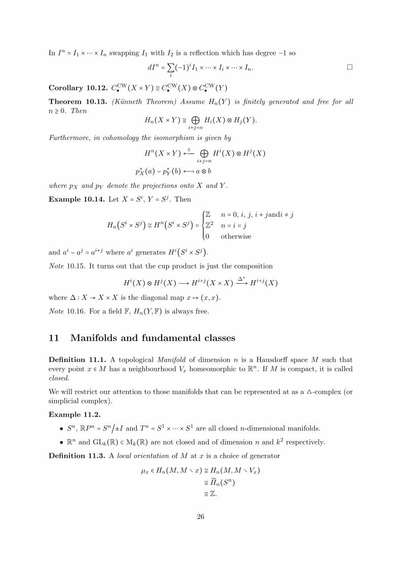
Proof.

01 11

02

12I2 = I1 × I2

dI1 = 11 − 01 and dI2 = 12 − 02

dI2 = I1 × 02 + 11 × I2 − I1 × 12 − 01 × I2

= dI1 × I2 − I1 × dI2

25

In In = I1 ×⋯ × In swapping I1 with I2 is a reflection which has degree −1 so

dIn =∑i

(−1)iI1 ×⋯ × Ii ×⋯ × In.

Corollary 10.12. CCW● (X × Y ) ≅ CCW

● (X)⊗CCW● (Y )

Theorem 10.13. (Kunneth Theorem) Assume Hn(Y ) is finitely generated and free for alln ≥ 0. Then

Hn(X × Y ) ≅ ⊕i+j=n

Hi(X)⊗Hj(Y ).

Furthermore, in cohomology the isomorphism is given by

Hn(X × Y ) ≅←ÐÐ ⊕i+j=n

H i(X)⊗Hj(X)

p∗X(a) ⌣ p∗Y (b)←Ð [ a⊗ b

where pX and pY denote the projections onto X and Y .

Example 10.14. Let X = Si, Y = Sj . Then

Hn(Si × Sj) ≅Hn(Si × Sj) =

⎧⎪⎪⎪⎪⎨⎪⎪⎪⎪⎩

Z n = 0, i, j, i + jandi ≠ jZ2 n = i = j0 otherwise

and ai ⌣ aj = ai+j where ai generates H i(Si × Sj).

Note 10.15. It turns out that the cup product is just the composition

H i(X)⊗Hj(X)Ð→H i+j(X ×X) ∆∗ÐÐ→H i+j(X)

where ∆ ∶X →X ×X is the diagonal map x↦ (x,x).

Note 10.16. For a field F, Hn(Y,F) is always free.

11 Manifolds and fundamental classes

Definition 11.1. A topological Manifold of dimension n is a Hausdorff space M such thatevery point x ∈M has a neighbourhood Vx homeomorphic to Rn. If M is compact, it is calledclosed.

We will restrict our attention to those manifolds that can be represented at as a △-complex (orsimplicial complex).

Example 11.2.

• Sn, RPn = Sn/±I and Tn = S1 ×⋯ × S1 are all closed n-dimensional manifolds.

• Rn and GLk(R) ⊂ Mk(R) are not closed and of dimension n and k2 respectively.

Definition 11.3. A local orientation of M at x is a choice of generator

µx ∈Hn(M,M ∖ x) ≅Hn(M,M ∖ Vx)≅ Hn(Sn)≅ Z.

26

An orientation of M is a locally consistent choice of x↦ µx:

Hn(M,M ∖ Vx)≅

yyrrrrrrr ≅%%LLLLLLL

Hn(M,M ∖ x) ≅ // Hn(M,M ∖ x)µx � // µy

xy Vx

M is called orientable if there exists an orientation for M .

Example 11.4. Sn is orientable but RP 2 = Mobius Band ∪ϕD2 is not.

Theorem 11.5. If M is orientable, closed and path connected of dimension n then

Hn(M) ≅Hn(M,M ∖ x) ≅ Z.

If M is not orientable and closed of dimension n then

Hn(M) = 0 and Hn(M ;F2) ≅ F2.

Proof. Let M be given as a ∆-complex. As M is closed, it is compact and hence it has onlyfinitely many n-simplices: γ1, . . . , γN . Define [M] ..= ∑i γi.

Over F2 each (n − 1)-simplex will appear twice in ∑i γi so ∂[M] = ∑i ∂γi = 0.

If M is orientable, the orientations of γi can be chosen such that over Z, ∂[M] = 0.

Definition 11.6. [M] is called the fundamental class of M if [M]↦ µx under the restriction

Hn(M) ≅ÐÐ→Hn(M,M ∖ x).

Example 11.7. [S2] = α+ − α− or [S2] = α− − α+α+↺

α−↺

Example 11.8. [F2] = ±(γ11 + γ12 − γ13 − γ14 + γ21 + γ22 − γ23 − γ24)γ11

γ12γ13

γ14

γ21

γ22 γ23

γ24

Example 11.9. [RP 2] = α + β ∈ C∆2 (RP 2;F2)

α

β

Definition 11.10. If f ∶M → N is a map between two n-dimensional oriented, closed manifolds,then the degree of f , deg(f) is determined by

f∗([M]) = deg(f)[N].

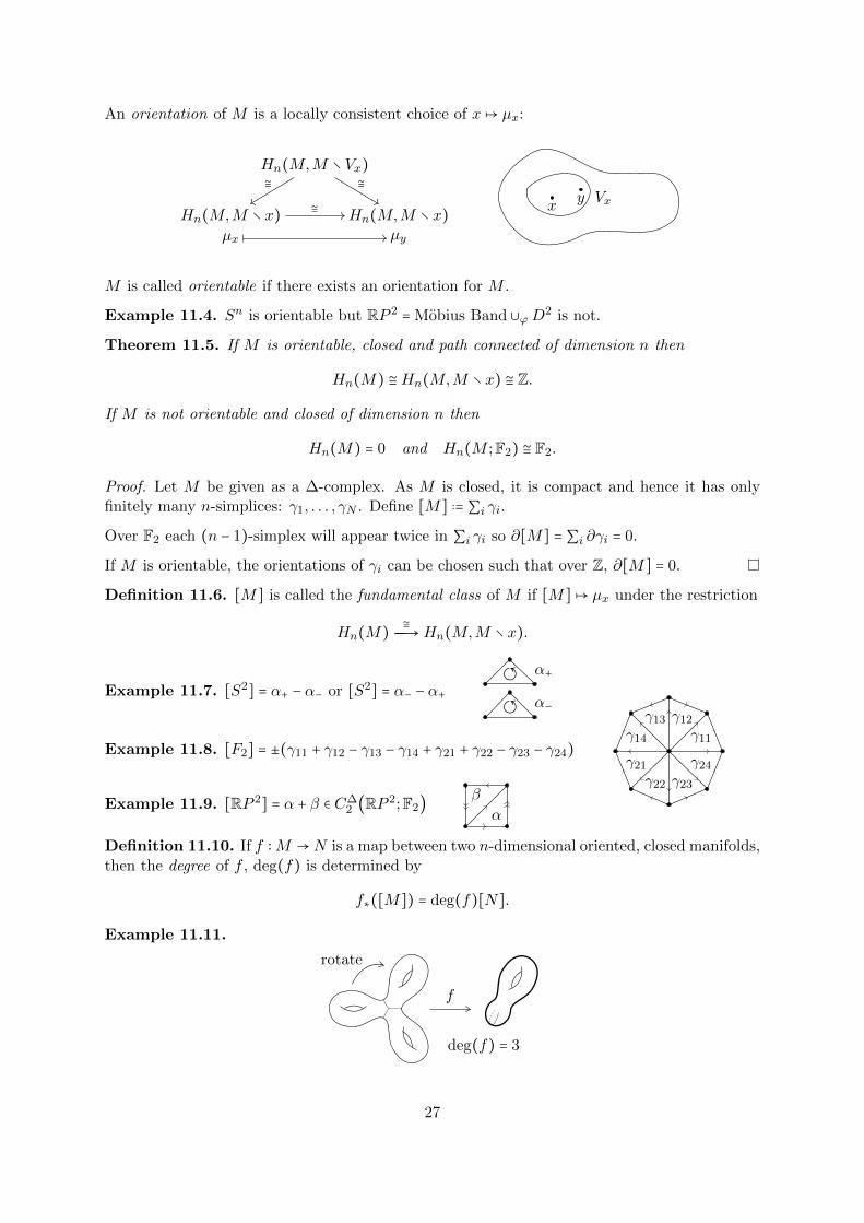
Example 11.11.

f

rotate

deg(f) = 3

27

Note 11.12. deg(f) is determined by the local degree.

Hn(M) f∗//

≅��

Hn(N)

≅��

Hn(M,M ∖ x)f∗∣x

// Hn(N,N ∖ f(x))

12 Duality

12.1 Poincare duality

Theorem 12.1. (Poincare duality) Let M be a closed, connected, oriented manifold of dimen-sion n. Then there exists an isomorphisms D ∶Hk(M)→Hn−k(M).

If M is closed, connected but not necessarily oriented, then there exists an isomorphism D ∶Hk(M ;Z/2)→Hn−k(M ;Z/2).

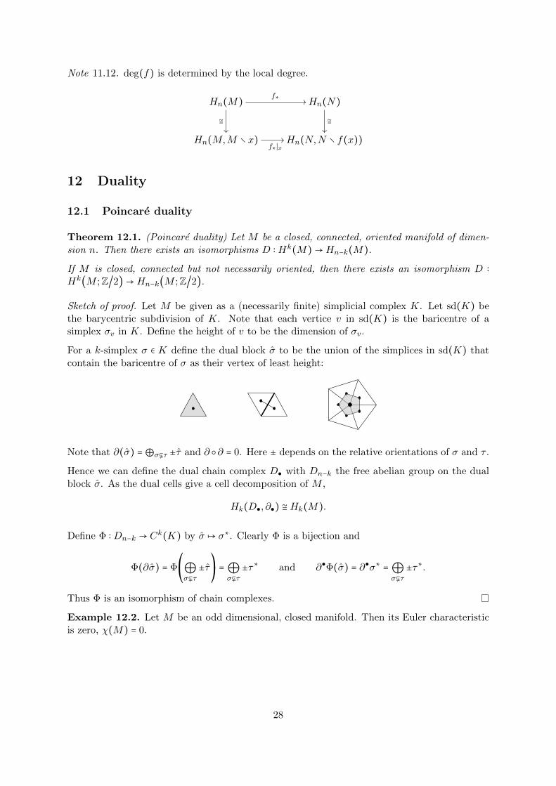
Sketch of proof. Let M be given as a (necessarily finite) simplicial complex K. Let sd(K) bethe barycentric subdivision of K. Note that each vertice v in sd(K) is the baricentre of asimplex σv in K. Define the height of v to be the dimension of σv.

For a k-simplex σ ∈ K define the dual block σ to be the union of the simplices in sd(K) thatcontain the baricentre of σ as their vertex of least height:

Note that ∂(σ) =⊕σ⊊τ ±τ and ∂ ○∂ = 0. Here ± depends on the relative orientations of σ and τ .

Hence we can define the dual chain complex D● with Dn−k the free abelian group on the dualblock σ. As the dual cells give a cell decomposition of M ,

Hk(D●, ∂●) ≅Hk(M).

Define Φ ∶Dn−k → Ck(K) by σ ↦ σ∗. Clearly Φ is a bijection and

Φ(∂σ) = Φ⎛⎝⊕σ⊊τ

±τ⎞⎠=⊕σ⊊τ

±τ∗ and ∂●Φ(σ) = ∂●σ∗ =⊕σ⊊τ

±τ∗.

Thus Φ is an isomorphism of chain complexes.

Example 12.2. Let M be an odd dimensional, closed manifold. Then its Euler characteristicis zero, χ(M) = 0.

28

12.2 Leftschetz duality

Definition 12.3. A manifold with boundary is a Hausdorff space M where every point x ∈Mhas an open neighbourhood homeomorphic to Rn or Rn−1 ×R≥0. Points with a neighbourhoodof the second form are boundary points and form the boundary ∂M of M .

Theorem 12.4. (Leftschetz duality) For n-dimensional manifolds with boundary there are iso-morphisms

Hn−k(M,∂M) ≅Hk(M) and Hn−k(M) ≅Hk(M,∂M).

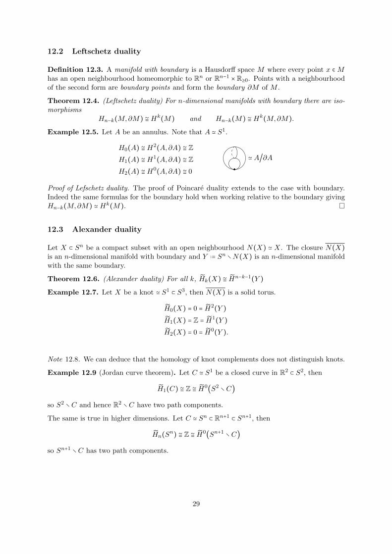
Example 12.5. Let A be an annulus. Note that A ≃ S1.

H0(A) ≅H2(A,∂A) ≅ ZH1(A) ≅H1(A,∂A) ≅ ZH2(A) ≅H0(A,∂A) ≅ 0

≃ A/∂A

Proof of Lefschetz duality. The proof of Poincare duality extends to the case with boundary.Indeed the same formulas for the boundary hold when working relative to the boundary givingHn−k(M,∂M) ≃Hk(M).

12.3 Alexander duality

Let X ⊂ Sn be a compact subset with an open neighbourhood N(X) ≃ X. The closure N(X)is an n-dimensional manifold with boundary and Y ..= Sn ∖N(X) is an n-dimensional manifoldwith the same boundary.

Theorem 12.6. (Alexander duality) For all k, Hk(X) ≅ Hn−k−1(Y )

Example 12.7. Let X be a knot ≃ S1 ⊂ S3, then N(X) is a solid torus.

H0(X) = 0 = H2(Y )H1(X) = Z = H1(Y )H2(X) = 0 = H0(Y ).

Note 12.8. We can deduce that the homology of knot complements does not distinguish knots.

Example 12.9 (Jordan curve theorem). Let C ≃ S1 be a closed curve in R2 ⊂ S2, then

H1(C) ≅ Z ≅ H0(S2 ∖C)

so S2 ∖C and hence R2 ∖C have two path components.

The same is true in higher dimensions. Let C ≃ Sn ⊂ Rn+1 ⊂ Sn+1, then

Hn(Sn) ≅ Z ≅ H0(Sn+1 ∖C)

so Sn+1 ∖C has two path components.

29

Proof of Alexander Duality. Let k < n − 1, then

Hn−k−1(Y ) =Hn−k−1(Y )=Hk+1(Y, ∂Y ) by Lefschetz duality

=Hk+1(Sk,N(X)) by excision

= Hk(N(X)) by long exact sequence as k < n − 1

= Hk(X)

Let k = n − 1, then

H0(Y )⊕Z =H0(Y )=Hn(Y, ∂Y ) by Lefschetz duality

=Hn(Sk,N(X)) by excision

= Hn − 1(N(X))⊕Z by (∗)

= Hn−1(X)⊕Z

0 // Hn(Sn)≅

''OOOOOOOOOOOOO// Hn(Sn,N(X))

��

// Hn−1(N(X)) // 0

Hn(Sn, Sn ∖∞)

(∗)

Let k ≥ n, then Hn−k−1(Y ) = 0 but so is Hk(X) ≅Hk(N(X)) as every component of N(X) has

non-empty boundary.

30