notes on the course “algebraic topology”botvinn/course.pdf · notes on the course “algebraic...
TRANSCRIPT

NOTES ON THE COURSE “ALGEBRAIC TOPOLOGY”
BORIS BOTVINNIK
Contents
1. Important examples of topological spaces 6
1.1. Euclidian space, spheres, disks. 6
1.2. Real projective spaces. 7
1.3. Complex projective spaces. 8
1.4. Grassmannian manifolds. 9
1.5. Flag manifolds. 9
1.6. Classic Lie groups. 9
1.7. Stiefel manifolds. 10
1.8. Surfaces. 11
2. Constructions 13
2.1. Product. 13
2.2. Cylinder, suspension 13
2.3. Glueing 14
2.4. Join 16
2.5. Spaces of maps, loop spaces, path spaces 16
2.6. Pointed spaces 17
3. Homotopy and homotopy equivalence 20
3.1. Definition of a homotopy. 20
3.2. Homotopy classes of maps 20
3.3. Homotopy equivalence. 20
3.4. Retracts 23
3.5. The case of “pointed” spaces 24
4. CW -complexes 25
Date:1

2 BORIS BOTVINNIK
4.1. Basic definitions 25
4.2. Some comments on the definition of a CW -complex 27
4.3. Operations on CW -complexes 27
4.4. More examples of CW -complexes 28
4.5. CW -structure of the Grassmanian manifolds 28
5. CW -complexes and homotopy 33
5.1. Borsuk’s Theorem on extension of homotopy 33
5.2. Cellular Approximation Theorem 35
5.3. Completion of the proof of Theorem 5.5 37
5.4. Fighting a phantom: Proof of Lemma 5.6 37
5.5. Back to the Proof of Lemma 5.6 39
5.6. First applications of Cellular Approximation Theorem 40
6. Fundamental group 43
6.1. General definitions 43
6.2. One more definition of the fundamental group 44
6.3. Dependence of the fundamental group on the base point 44
6.4. Fundamental group of circle 44
6.5. Fundamental group of a finite CW -complex 46
6.6. Theorem of Seifert and Van Kampen 49
7. Covering spaces 52
7.1. Definition and examples 52
7.2. Theorem on covering homotopy 52
7.3. Covering spaces and fundamental group 53
7.4. Observation 54
7.5. Lifting to a covering space 54
7.6. Classification of coverings over given space 56
7.7. Homotopy groups and covering spaces 57
7.8. Lens spaces 58
8. Higher homotopy groups 60
8.1. More about homotopy groups 60
8.2. Dependence on the base point 60
NOTES ON THE COURSE “ALGEBRAIC TOPOLOGY” 3
8.3. Relative homotopy groups 61
9. Fiber bundles 65
9.1. First steps toward fiber bundles 65
9.2. Constructions of new fiber bundles 67
9.3. Serre fiber bundles 70
9.4. Homotopy exact sequence of a fiber bundle 73
9.5. More on the groups πn(X,A; x0) 75
10. Suspension Theorem and Whitehead product 76
10.1. The Freudenthal Theorem 76
10.2. First applications 80
10.3. A degree of a map Sn → Sn 80
10.4. Stable homotopy groups of spheres 80
10.5. Whitehead product 80
11. Homotopy groups of CW -complexes 86
11.1. Changing homotopy groups by attaching a cell 86
11.2. Homotopy groups of a wedge 88
11.3. The first nontrivial homotopy group of a CW -complex 88
11.4. Weak homotopy equivalence 89
11.5. Cellular approximation of topological spaces 93
11.6. Eilenberg-McLane spaces 94
11.7. Killing the homotopy groups 95
12. Homology groups: basic constructions 98
12.1. Singular homology 98
12.2. Chain complexes, chain maps and chain homotopy 99
12.3. First computations 100
12.4. Relative homology groups 101
12.5. Relative homology groups and regular homology groups 104
12.6. Excision Theorem 107
12.7. Mayer-Vietoris Theorem 108
13. Homology groups of CW -complexes 110
13.1. Homology groups of spheres 110
4 BORIS BOTVINNIK
13.2. Homology groups of a wedge 111
13.3. Maps g :∨
α∈ASnα→
∨
β∈BSnβ 111
13.4. Cellular chain complex 112
13.5. Geometric meaning of the boundary homomorphism ∂≀
q 115
13.6. Some computations 117
13.7. Homology groups of RPn 117
13.8. Homology groups of CPn , HPn 118
14. Homology and homotopy groups 120
14.1. Homology groups and weak homotopy equivalence 120
14.2. Hurewicz homomorphism 122
14.3. Hurewicz homomorphism in the case n = 1 124
14.4. Relative version of the Hurewicz Theorem 125
15. Homology with coefficients and cohomology groups 127
15.1. Definitions 127
15.2. Basic propertries of H∗(−;G) and H∗(−;G) 128
15.3. Coefficient sequences 129
15.4. The universal coefficient Theorem for homology groups 130
15.5. The universal coefficient Theorem for cohomology groups 132
15.6. The Kunneth formula 136
15.7. The Eilenberg-Steenrod Axioms. 139
16. Some applications 141
16.1. The Lefschetz Fixed Point Theorem 141
16.2. The Jordan-Brouwer Theorem 143
16.3. The Brouwer Invariance Domain Theorem 146
16.4. Borsuk-Ulam Theorem 146
17. Cup product in cohomology. 149
17.1. Ring structure in cohomology 149
17.2. Definition of the cup-product 149
17.3. Example 152
17.4. Relative case 153
NOTES ON THE COURSE “ALGEBRAIC TOPOLOGY” 5
17.5. External cup product 154
18. Cap product and the Poincare duality. 159
18.1. Definition of the cap product 159
18.2. Crash course on manifolds 160
18.3. Poincare isomorphism 162
18.4. Some computations 165
19. Hopf Invariant 166
19.1. Whitehead product 166
19.2. Hopf invariant 166
20. Elementary obstruction theory 171
20.1. Eilenberg-MacLane spaces and cohomology operations 171
20.2. Obstruction theory 173
20.3. Proof of Theorem 20.3 177
20.4. Stable Cohomology operations and Steenrod algebra 179
21. Cohomology of some Lie groups and Stiefel manifolds 180
21.1. Stiefel manifolds 180
6 BORIS BOTVINNIK
1. Important examples of topological spaces
1.1. Euclidian space, spheres, disks. The notations Rn , Cn have usual meaning through-out the course. The space Cn is identified with R2n by the correspondence
(x1 + iy1, . . . , yn + ixn)←→ (x1, y1, . . . , xn, yn).
The unit sphere in Rn+1 centered in the origin is denoted by Sn , the unit disk in Rn by Dn ,and the unit cube in Rn by In . Thus Sn−1 is the boundary of the disk Dn . Just in case wegive these spaces in coordinates:
(1)
Sn−1 = (x1, . . . , xn) ∈ Rn | x21 + · · ·+ x2
n = 1 ,
Dn = (x1, . . . , xn) ∈ Rn | x21 + · · ·+ x2
n ≤ 1 ,
In = (x1, . . . , xn) ∈ Rn | 0 ≤ xj ≤ 1, j = 1, . . . , n .The symbol R∞ is a union (direct limit) of the embeddings
R1 ⊂ R2 ⊂ · · · ⊂ Rn ⊂ · · · .Thus a point x ∈ R∞ is a sequence of points x = (x1, . . . , xn, . . .), where xn ∈ R and xj = 0for j greater then some k . Topology on R∞ is determined as follows. A set F ⊂ R∞ isclosed, if each intersection F ∩Rn is closed in Rn . In a similar way we define the spaces C∞
and S∞ .
Exercise 1.1. Let x(1) = (a1, 0, . . . , 0, . . .), . . ., x(n) = (0, 0, . . . , an, . . .), . . . be a sequence ofelements in R∞ . Prove that the sequence
x(n)
converges in R∞ if and only if the sequenceof numbers an is finite.
Probably you already know the another version of infinite-dimensional real space, namely theHilbert space ℓ2 (which is the set of sequences xn so that the series
∑n xn converges). The
space ℓ2 is a metric space, where the distance ρ(xn , yn) is defined as
ρ(xn , yn) =√∑
n(yn − xn)2.
Clearly there is a natural map R∞ −→ ℓ2 .
Remark. The optional exercises are labeled by ∗ .
Exercise 1.2. Is the above map R∞ −→ ℓ2 homeomorphism or not?
Consider the unit cube I∞ in the spaces R∞ , ℓ2 , i.e. I∞ = xn | 0 ≤ xn ≤ 1 .Exercise 1.3. Prove or disprove that the cube I∞ is compact space (in R∞ or ℓ2 ).
We are going to play a little bit with the sphere Sn .
Claim 1.1. A punctured sphere Sn \ x0 is homeomorphic to Rn .
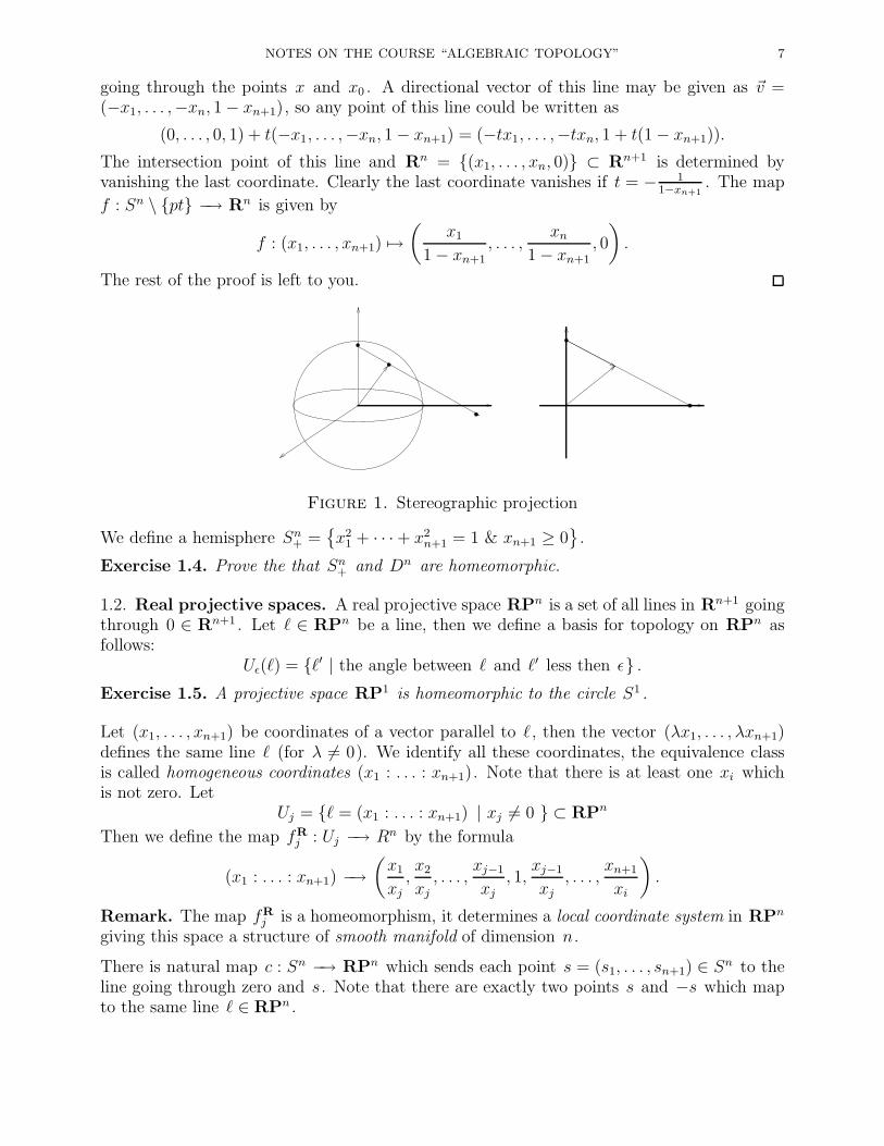
Proof. We construct a map f : Sn \x0 −→ Rn which is known as stereographic projection.Let Sn be given as above (1). Let the point x0 be the North Pole, so it has the coordinates(0, . . . , 0, 1) ∈ Rn+1 . Consider a point x = (x1, . . . , xn+1) ∈ Sn , x 6= x0 , and the line
NOTES ON THE COURSE “ALGEBRAIC TOPOLOGY” 7
going through the points x and x0 . A directional vector of this line may be given as ~v =(−x1, . . . ,−xn, 1− xn+1), so any point of this line could be written as
(0, . . . , 0, 1) + t(−x1, . . . ,−xn, 1− xn+1) = (−tx1, . . . ,−txn, 1 + t(1− xn+1)).
The intersection point of this line and Rn = (x1, . . . , xn, 0) ⊂ Rn+1 is determined byvanishing the last coordinate. Clearly the last coordinate vanishes if t = − 1
1−xn+1. The map
f : Sn \ pt −→ Rn is given by
f : (x1, . . . , xn+1) 7→(
x1
1− xn+1, . . . ,
xn1− xn+1
, 0
).
The rest of the proof is left to you.
Figure 1. Stereographic projection
We define a hemisphere Sn+ =x2
1 + · · ·+ x2n+1 = 1 & xn+1 ≥ 0
.
Exercise 1.4. Prove the that Sn+ and Dn are homeomorphic.
1.2. Real projective spaces. A real projective space RPn is a set of all lines in Rn+1 goingthrough 0 ∈ Rn+1 . Let ℓ ∈ RPn be a line, then we define a basis for topology on RPn asfollows:
Uǫ(ℓ) = ℓ′ | the angle between ℓ and ℓ′ less then ǫ .Exercise 1.5. A projective space RP1 is homeomorphic to the circle S1 .
Let (x1, . . . , xn+1) be coordinates of a vector parallel to ℓ, then the vector (λx1, . . . , λxn+1)defines the same line ℓ (for λ 6= 0). We identify all these coordinates, the equivalence classis called homogeneous coordinates (x1 : . . . : xn+1). Note that there is at least one xi whichis not zero. Let
Uj = ℓ = (x1 : . . . : xn+1) | xj 6= 0 ⊂ RPn
Then we define the map fR
j : Uj −→ Rn by the formula
(x1 : . . . : xn+1) −→(x1
xj,x2
xj, . . . ,
xj−1
xj, 1,
xj−1
xj, . . . ,
xn+1
xi
).
Remark. The map fR
j is a homeomorphism, it determines a local coordinate system in RPn
giving this space a structure of smooth manifold of dimension n.
There is natural map c : Sn −→ RPn which sends each point s = (s1, . . . , sn+1) ∈ Sn to theline going through zero and s. Note that there are exactly two points s and −s which mapto the same line ℓ ∈ RPn .
8 BORIS BOTVINNIK
We have a chain of embeddings
RP1 ⊂ RP2 ⊂ · · · ⊂ RPn ⊂ RPn+1 ⊂ · · · ,
we define RP∞ =⋃n≥1 RPn with the limit topology (similarly to the above case of R∞ ).
1.3. Complex projective spaces. Let CPn be the space of all complex lines in the complexspace Cn+1 . In the same way as above we define homogeneous coordinates (z1 : . . . : zn+1)for each complex line ℓ ∈ CPn , and the “local coordinate system”:
Ui = ℓ = (z1 : . . . : zn) | zi 6= 0 ⊂ CPn.
Clearly there is a homemorphism fC
i : Ui −→ Cn+1 .
Exercise 1.6. Prove that the projective space CP1 is homeomorphic to the sphere S2 .
Consider the sphere S2n+1 ⊂ Cn+1 . Each point
z = (z1, . . . , zn+1) ∈ S2n−1, |z1|2 + · · ·+ |zn+1|2 = 1
of the sphere S2n+1 determines a line ℓ = (z1 : . . . : zn+1) ∈ CPn . Observe that the pointeiϕz = (eiϕz1, . . . , e
iϕzn+1) ∈ S2n+1 determines the same complex line ℓ ∈ CPn . We havedefined the map g(n) : S2n+1 −→ CPn .
Exercise 1.7. Prove that the map g(n) : S2n+1 −→ CPn has a property that g(n)−1(ℓ) = S1
for any ℓ ∈ CPn .
The case n = 1 is very interesting since CP1 = S2 , here we have the map g(1) : S3 −→ S2
where g(1)−1(x) = S1 for any x ∈ S2 . This map is the Hopf map, it gives very importantexample of nontrivial map S3 −→ S2 . Before this map was discovered by Hopf, peoplethought that there are no nontrivial maps Sk −→ Sn for k > n (“trivial map” means a maphomotopic to the constant map).
Exercise 1.8. Prove that RPn , CPn are compact and connected spaces.
Besides the reals R and complex numbers C there are quaternion numbers H . Recall thatq ∈ H may be thought as a sum q = a + ib + jc + kd , where a, b, c, d ∈ R , and the symbolsi, j, k satisfy the identities:
i2 = j2 = k2 = −1, ij = −ji = k, jk = −kj = i, ki = −ik = j.
Then two quaternions q1 = a1 + ib1 +jc1 +kd1 and q2 = a2 + ib2 +jc2 +kd2 may be multipliedusing these identies. The product here is not commutative, however one can choose left orright multiplication to define a line in Hn+1 . A set of all quaternionic lines in Hn+1 is thequaternion projective space HPn .
Exercise 1.9. Give details of the above definition. In particular, check that the space HPn
is well-defined. Identify the quaternionic line HP1 with some well-known topological space.
NOTES ON THE COURSE “ALGEBRAIC TOPOLOGY” 9
1.4. Grassmannian manifolds. These spaces generalize the projective spaces. Indeed, thespace G(n, k) is a space of all k -dimensional vector subpaces of Rn with natural topology.Clearly G(n, 1) = RP1 . It is not difficult to introduce local coordinates in G(n, k). Letπ ∈ G(n, k) be a k -plane. Choose k linearly independent vectors v1, . . . , vk generating πand write their coordinates in the standard basis e1, . . . , en of Rn :
A =
a11 · · · a1n...
......
ak1 · · · akn
Since the vectors v1, . . . , vk are linearly independent there exist k columns of the matrix Awhich are linearly independent as well. In other words, there are indices i1, . . . , ik so that aprojection of the plane π on the k -plane 〈ei1 , . . . , eik〉 generated by the coordinate vectorsei1 , . . . , eik is a linear isomorphism. Now it is easy to introduce local coordinates on theGrassmanian manifold G(n, k). Indeed, choose the indices i1, . . . , ik , 1 ≤ i1 < · · · < ik ≤ n,and consider all k -planes π ∈ G(n, k) so that the projection of π on the plane 〈ei1 , . . . , eik〉is a linear isomorphism. We denote this set of k -planes by Ui1,...,ik .
Exercise 1.10. Construct a homeomorphism fi1,...,ik : Ui1,...,ik −→ Rk(n−k) .
The result of this exercise shows that the Grassmannian manifold G(n, k) is a smooth manifoldof dimension k(n−k). The projective spaces and Grassmannian manifolds are very importantexamples of spaces which we will see many times in our course.
Exercise 1.11. Define a complex Grassmannian manifold CG(n, k) and construct a localcoordinate system for CG(n, k). In particular, find its dimension.
We have a chain of spaces:
G(k, k) ⊂ G(k + 1, k) ⊂ · · · ⊂ G(n, k) ⊂ G(n + 1, k) ⊂ · · · .Let G(∞, k) be the union (inductive limit) of these spaces. The topology of G(∞, k) isgiven in the same way as to R∞ : a set F ⊂ G(∞, k) is closed if and only if the intersectionF ∩G(n, k) is closed for each n. This topology is known as a topology of an inductive limit.
Exercise 1.12. Prove that the Grassmannian manifolds G(n, k) and CG(n, k) are compactand connected.
1.5. Flag manifolds. Here we just mention these examples without further considerations(we are not ready for this yet). Let 1 ≤ k1 < · · · < ks ≤ n− 1. A flag of the type (k1, . . . , ks)is a chain of vector subspaces V1 ⊂ · · · ⊂ Vs of Rn such that dimVi = ki . A set of flags ofthe given type is the flag manifold F (n; k1, . . . , ks). Hopefully we shall return to these spaces:they are very interesting and popular creatures.
1.6. Classic Lie groups. The first example here is the group GL(Rn) of nondegeneratedlinear transformations of Rn . Once we choose a basis e1, . . . , en of Rn , each element A ∈GL(Rn) may be identified with an n× n matrix A with detA 6= 0. Clearly we may identifythe space of all n × n matrices with the space Rn2
. The determinant gives a continuousfunction det : Rn2 −→ R , and the space GL(Rn) is an open subset of Rn2
:
GL(Rn) = Rn2 \ det−1(0).

10 BORIS BOTVINNIK
In particular, this identification defines a topology on GL(Rk). In the same way one mayconstruct an embedding GL(Cn) ⊂ Cn2
. The orthogonal and special orthogonal groups O(k),SO(k) are subgroups of GL(Rk), and the groups U(k), SU(k) are subgroups of GL(Ck).(Recall that O(n) (or U(n)) is a group of those linear transformations of Rn (or Cn ) whichpreserve a Euclidian (or Hermitian) metric on Rn (or Cn ), and the groups SO(k) and SU(k)are subgroups of O(k) and U(k) of matrices with the determinant 1.)
Exercise 1.13. Prove that SO(2) and U(1) are homeomorphic to S1 , and that SO(3) ishomeomorphic to RP3 .
Hint: To prove that SO(3) is homeomorphic to RP3 you have to analyze SO(3): the keyfact is the geometric description of an orthogonal transformation α ∈ SO(3), it is given byrotating a plane (by an angle ϕ) about a line ℓ perpendicular to that plane. You should use theline ℓ and the angle ϕ as major parameters to construct a homeomorphism SO(3)→ RP3 ,where it is important to use a particular model of RP3 , namely a disk D3 where one identifiesthe opposite points on S2 = ∂D3 ⊂ D3 .
Exercise 1.14. Prove that the spaces O(n), SO(n), U(n), SU(n) are compact.
Exercise 1.15. Prove that the space O(n) has two path-connected components, and that thespaces SO(n), U(n), SU(n) are path-connected.
Exercise 1.16. Prove that each matrix A ∈ SU(2) may be presented as:
A =
(α β−β α
),where α, β ∈ C, |α|2 + |β|2 = 1
Use this presentation to prove that SU(2) is homeomorphic to S3 .
It is important to emphasize that the classic groups O(n), SO(n), U(n), SU(n) are allmanifolds, i.e. for each point α there there exists an open neighborhood homeomorphic to aEuclidian space.
Exercise 1.17. Prove that the space for any point α ∈ SO(n) there exists an open neighbor-
hood homeomorphic to the Euclidian space of the dimension n(n−1)2
.
Exercise 1.18. Prove that the spaces U(n), SU(n) are manifolds and find their dimension.
The next set of examples is also very important.
1.7. Stiefel manifolds. Again, we consider the vector space Rn . We call vectors v1, . . . , vka k -frame if they are linearly independent. A k -frame v1, . . . , vk is called an orthonormalk -frame if the vectors v1, . . . , vk are of unit length and orthogonal to each other. The spaceof all orthonormal k -frames in Rn is denoted by V (n, k). There are analogous complex andquaternionic versions of these spaces, they are denoted as CV (n, k) and HV (n, k) respec-tively. Here is an exercise where your knowledge of basic linear algebra may be crucial:
Exercise 1.19. Prove the following homeomorphisms: V (n, n) ∼= O(n), V (n, n − 1) ∼=SO(n), CV (n, n) ∼= U(n), CV (n, n − 1) ∼= SU(n), V (n, 1) ∼= Sn−1 , CV (n, 1) ∼= S2n−1 ,HV (n, 1) ∼= S4n−1 .

NOTES ON THE COURSE “ALGEBRAIC TOPOLOGY” 11
We note that the group O(n) acts on the spaces V (n, k) and G(n, k): indeed, if α ∈ O(n)and v1, . . . , vk is an orthonormal k -frame, then α(v1), . . . , α(vk) is also an orthonormal k -frame. As for the Grassmannian manifold, one can easily see that α(Π) is a k -dimensionalsubspace in Rn if Π is.
The group O(n) contains a subgroup O(j) which acts on Rj ⊂ Rn , where Rj = 〈e1, . . . , ej〉is generated by the first j vectors e1, . . . , ej of the standard basis e1, . . . , en of Rn . SimilarlyU(n) acts on the spaces CG(n, k) and CV (n, k), and U(j) is a subgroup of U(n).
Exercise 1.20. Prove the following homeomorphisms:
(a) Sn−1 ∼= O(n)/O(n− 1) ∼= SO(n)/SO(n− 1),
(b) S2n−1 ∼= U(n)/U(n− 1) ∼= SU(n)/SU(n− 1),
(c) G(n, k) ∼= O(n)/O(k)×O(n− k),
(c) CG(n, k) ∼= U(n)/U(k) × U(n− k).
We note here that O(k)× O(n− k) is a subgroup of O(n) of orthogonal matrices with twodiagonal blocks of the sizes k × k and (n− k)× (n− k) and zeros otherwise.
There is also the following natural action of the orthogonal group O(k) on the Stieffelmanifold V (n, k). Let v1, . . . , vk be an orthonormal k -frame then O(k) acts on the spaceV = 〈v1, . . . , vk〉 , in particular, if α ∈ O(k), then α(v1), . . . , α(vk) is also an orthonormalk -frame. Similarly there is a natural action of U(k) on CV (n, k).
Exercise 1.21. Prove that the above actions of O(k) on V (n, k) and of U(k) on CV (n, k)are free.
Exercise 1.22. Prove the following homeomorphisms:
(a) V (n, k)/O(k) ∼= G(n, k),
(b) CV (n, k)/U(k) ∼= CG(n, k).
There are obvious maps V (n, k)p−→ G(n, k), CV (n, k)
p−→ CG(n, k) (where each orthonor-mal k -frame v1, . . . , vk maps to the k -plane π = 〈v1, . . . , vk〉 generated by this frame). It iseasy to see that the inverse image p−1(π) may be identified with O(k) (in the real case) andU(k) (in the complex case). We shall return to these spaces later on. In particular, we shalldescribe a cell-structure of these spaces and compute their homology and cohomology groups.
1.8. Surfaces. Here I refer to Chapter 1 of Massey, Algebraic topology, for details. I wouldlike for you to read this Chapter carefully even though most of you have seen this materialbefore. Here I briefly remind some constructions and give exercises. The section 4 of thereffered Massey book gives the examples of surfaces. In particular, the torus T 2 is describedin three different ways:
(a) A product S1 × S1 .

12 BORIS BOTVINNIK
(b) A subspace of R3 given by:
(x, y, z) ∈ R3 | (√x2 + y2 − 2)2 + z2 = 1
.
(c) A unit square I2 = (x, y) ∈ R2 | 0 ≤ x ≤ 1, 0 ≤ y ≤ 1 with the identification:
(x, 0) ≡ (x, 1) (0, y) ≡ (1, y) for all 0 ≤ x ≤ 1, 0 ≤ y ≤ 1.
Exercise 1.23. Prove that the spaces described in (a), (b), (c) are indeed homeomorphic.
T 2 RP2
⇐⇒aa
b
b
aa
b
b
Figure 2. Torus and projective plane
The next surface we want to become our best friend is the projective space RP2 . Earlier wedefined RP2 as a space of lines in R3 going through the origin.
Exercise 1.24. Prove that the projective plane RP2 is homeomorphic to the following spaces:
(a) The unit disk D2 = (x, y) ∈ R2 | x2 + y2 ≤ 1 with the opposite points (x, y) ≡(−x,−y) of the circle S1 = (x, y) ∈ R2 | x2 + y2 = 1 ⊂ D2 have been identified.
(b) The unit square, see Fig. 3, with the arrows a and b identified as it is shown.(c) The Mebius band which boundary (the circle) is identified with the boundary of the
disk D2 , see Fig. 3.
M e D2
aa a a
b
b
The Klein bottleFigure 3
Here the Mebius band is constructed from a square by identifying the arrows a. The Kleinbottle Kl2 may be described as a square with arrows identified as it is shown in Fig. 3.
Exercise 1.25. Prove that the Klein bottle Kl2 is homeomorphic to the union of two Mebiusbands along the circle.
Massey carefully defines connected sum S1#S2 of two surfaces S1 and S2 .
Exercise 1.26. Prove that Kl2#RP2 is homeomorphic to RP2#T 2 .
Exercise 1.27. Prove that Kl2#Kl2 is homeomorphic to Kl2 .
Exercise 1.28. Prove that RP2#RP2 is homeomorphic to Kl2 .
NOTES ON THE COURSE “ALGEBRAIC TOPOLOGY” 13
2. Constructions
2.1. Product. Recall that a product X × Y of X , Y is a set of pairs (x, y), x ∈ X, y ∈ Y .If X , Y are topological spaces then a basis for product topology on X × Y is given by theproducts U × V , where U ⊂ X , V ⊂ Y are open. Here are the first examples:
Example. The torus T n = S1 × · · · × S1 . Note that the torus T n may be identified withU(1)× · · · × U(1) ⊂ U(n) (diagonal orthogonal complex matrices).
Exercise 2.1. Consider the surface X in S5 , given by the equation
x1x6 − x2x5 + x3x4 = 0
(where S5 ⊂ R6 is given by x21 + · · ·+ x2
6 = 1). Prove that X ∼= S2 × S2 .
Exercise 2.2. Prove that the space SO(4) is homeomorphic to S3 ×RP3 .
Hint: Consider carefully the map SO(4) −→ S3 = SO(4)/SO(3) and use the fact that S3
has a natural group structure: it is a group of unit quaternions. It should be emphasized thatit is not true that SO(n) ∼= Sn−1 × SO(n− 1) if n > 4.
We note also that there are standard projections X × Y prX−−→ X and X × Y prY−−→ Y , and togive a map f : Z −→ X×Y is the same as to give two maps fX : Z −→ X and fY : Z −→ Y .
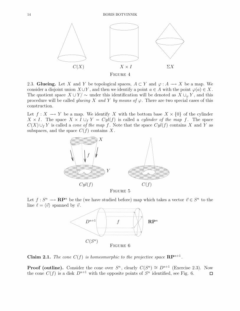
2.2. Cylinder, suspension. Let I = [0, 1] ⊂ R . The space X × I is called a cylinder overX , and the subspaces X × 0 , X × 1 are the bottom and top “bases”. Now we willconstruct new spaces out of the cylinder X × I .
Remark: quotient topology. Let “∼” be an equivalence relation on the topological spaceX . We denote by X/ ∼ the set of equivalence classes. There is a natural map (not continuosso far) p : X −→ X/ ∼. We define the following topology on X/ ∼: the set U ⊂ X/ ∼ isopen if and only if p−1(U) is open. This topology is called a quotient topology.
The first example: let A ⊂ X be a closed set. Then we define the relation “∼” on X asfollows ([ ] denote an equivalence class):
[x] =
x if x /∈ A,A if x ∈ A.
The space X/ ∼ is denoted by X/A.
The space C(X) = X × I/X ×1 is a cone over X . A suspention ΣX over X is the spaceC(X)/X × 0.
Exercise 2.3. Prove that the spaces C(Sn) and ΣSn are homeomorphic to Dn+1 and Sn+1
respectively.
Here is a picture of these spaces:
14 BORIS BOTVINNIK
C(X) X × I ΣX
Figure 4
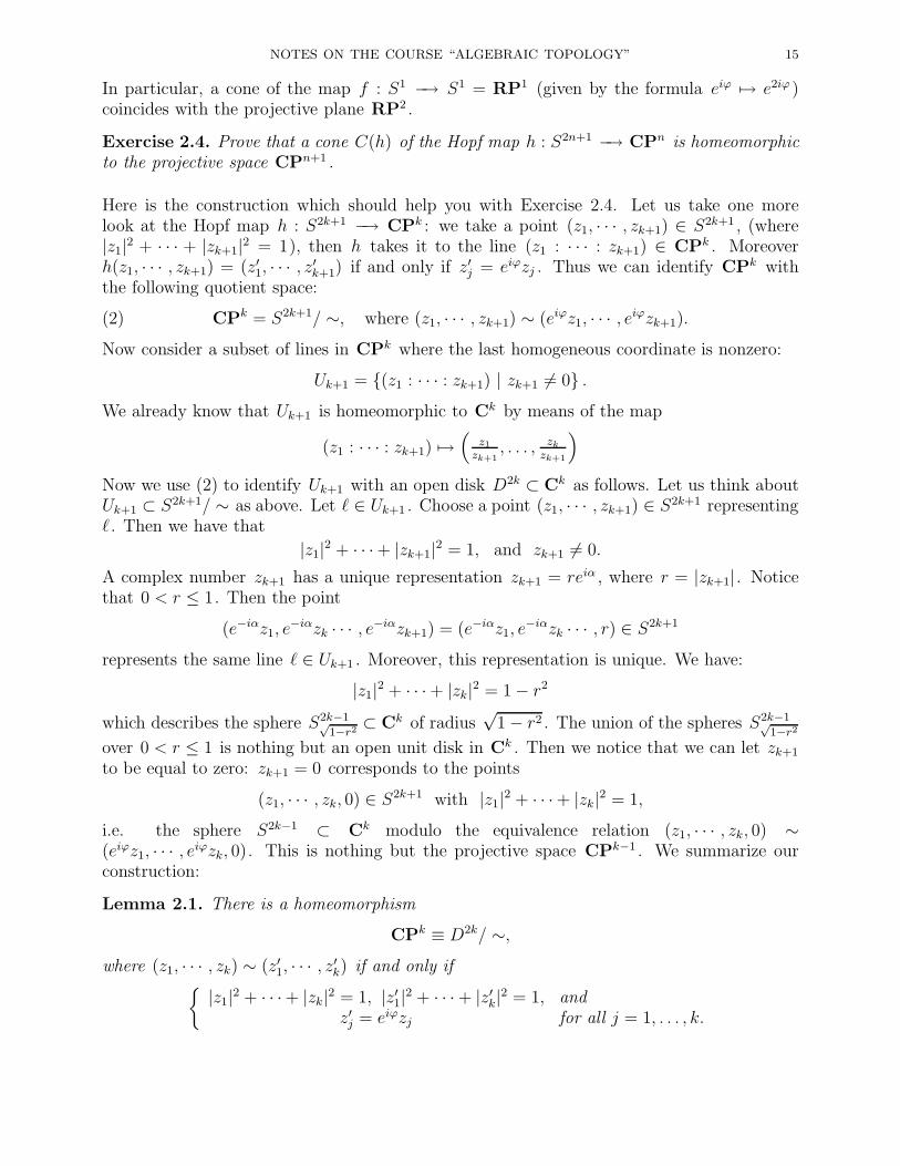
2.3. Glueing. Let X and Y be topological spaces, A ⊂ Y and ϕ : A −→ X be a map. Weconsider a disjoint union X∪Y , and then we identify a point a ∈ A with the point ϕ(a) ∈ X .The quotient space X ∪ Y/ ∼ under this identification will be denoted as X ∪ϕ Y , and thisprocedure will be called glueing X and Y by means of ϕ . There are two special cases of thisconstruction.
Let f : X −→ Y be a map. We identify X with the bottom base X × 0 of the cylinderX × I . The space X × I ∪f Y = Cyl(f) is called a cylinder of the map f . The spaceC(X)∪f Y is called a cone of the map f . Note that the space Cyl(f) contains X and Y assubspaces, and the space C(f) contains X .
Y
X
f
Cyl(f) C(f)
Figure 5
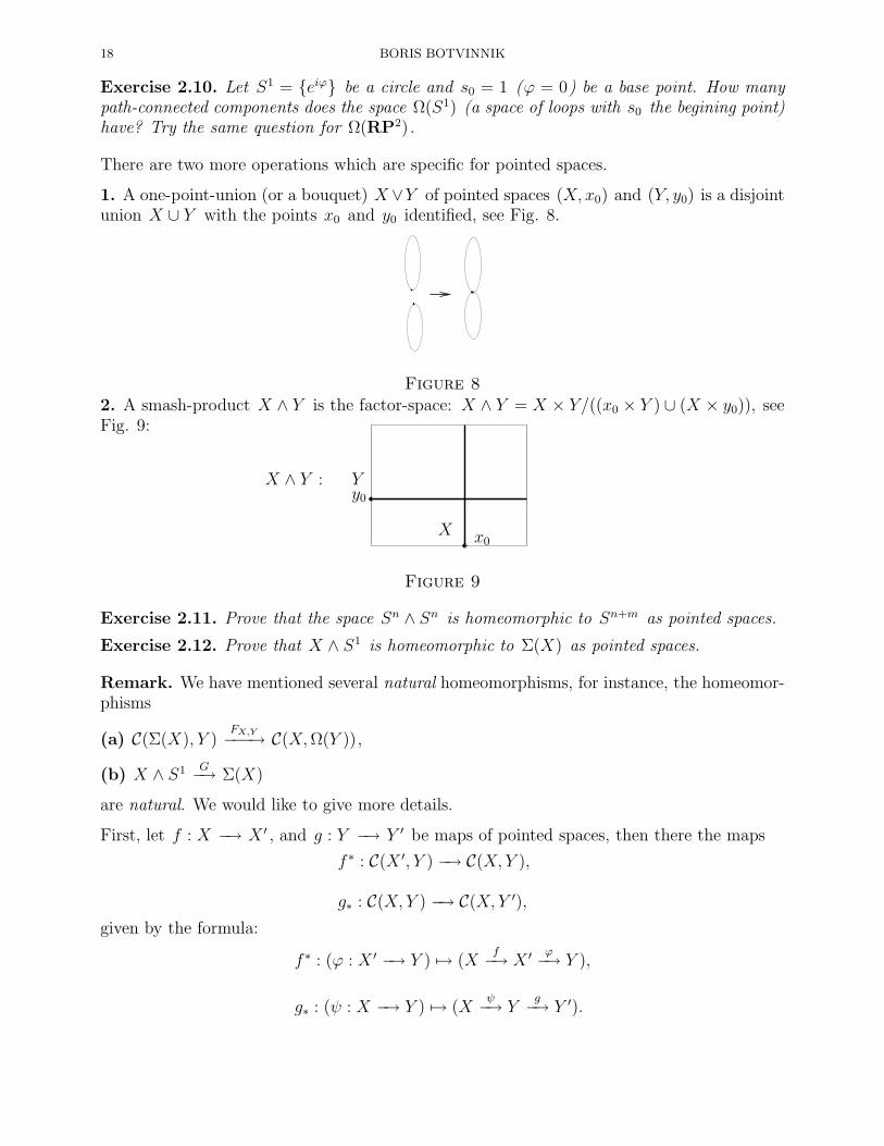
Let f : Sn −→ RPn be the (we have studied before) map which takes a vector ~v ∈ Sn to theline ℓ = 〈~v〉 spanned by ~v .
Dn+1
C(Sn)
f RPn
Figure 6
Claim 2.1. The cone C(f) is homeomorphic to the projective space RPn+1 .
Proof (outline). Consider the cone over Sn , clearly C(Sn) ∼= Dn+1 (Exercise 2.3). Nowthe cone C(f) is a disk Dn+1 with the opposite points of Sn identified, see Fig. 6.
NOTES ON THE COURSE “ALGEBRAIC TOPOLOGY” 15
In particular, a cone of the map f : S1 −→ S1 = RP1 (given by the formula eiϕ 7→ e2iϕ )coincides with the projective plane RP2 .
Exercise 2.4. Prove that a cone C(h) of the Hopf map h : S2n+1 −→ CPn is homeomorphicto the projective space CPn+1 .
Here is the construction which should help you with Exercise 2.4. Let us take one morelook at the Hopf map h : S2k+1 −→ CPk : we take a point (z1, · · · , zk+1) ∈ S2k+1 , (where|z1|2 + · · · + |zk+1|2 = 1), then h takes it to the line (z1 : · · · : zk+1) ∈ CPk . Moreoverh(z1, · · · , zk+1) = (z′1, · · · , z′k+1) if and only if z′j = eiϕzj . Thus we can identify CPk withthe following quotient space:
(2) CPk = S2k+1/ ∼, where (z1, · · · , zk+1) ∼ (eiϕz1, · · · , eiϕzk+1).
Now consider a subset of lines in CPk where the last homogeneous coordinate is nonzero:
Uk+1 = (z1 : · · · : zk+1) | zk+1 6= 0 .We already know that Uk+1 is homeomorphic to Ck by means of the map
(z1 : · · · : zk+1) 7→(
z1zk+1
, . . . , zk
zk+1
)
Now we use (2) to identify Uk+1 with an open disk D2k ⊂ Ck as follows. Let us think aboutUk+1 ⊂ S2k+1/ ∼ as above. Let ℓ ∈ Uk+1 . Choose a point (z1, · · · , zk+1) ∈ S2k+1 representingℓ. Then we have that
|z1|2 + · · ·+ |zk+1|2 = 1, and zk+1 6= 0.
A complex number zk+1 has a unique representation zk+1 = reiα , where r = |zk+1| . Noticethat 0 < r ≤ 1. Then the point
(e−iαz1, e−iαzk · · · , e−iαzk+1) = (e−iαz1, e
−iαzk · · · , r) ∈ S2k+1
represents the same line ℓ ∈ Uk+1 . Moreover, this representation is unique. We have:
|z1|2 + · · ·+ |zk|2 = 1− r2
which describes the sphere S2k−1√1−r2 ⊂ Ck of radius
√1− r2 . The union of the spheres S2k−1√
1−r2over 0 < r ≤ 1 is nothing but an open unit disk in Ck . Then we notice that we can let zk+1
to be equal to zero: zk+1 = 0 corresponds to the points
(z1, · · · , zk, 0) ∈ S2k+1 with |z1|2 + · · ·+ |zk|2 = 1,
i.e. the sphere S2k−1 ⊂ Ck modulo the equivalence relation (z1, · · · , zk, 0) ∼(eiϕz1, · · · , eiϕzk, 0). This is nothing but the projective space CPk−1 . We summarize ourconstruction:
Lemma 2.1. There is a homeomorphism
CPk ≡ D2k/ ∼,where (z1, · · · , zk) ∼ (z′1, · · · , z′k) if and only if
|z1|2 + · · ·+ |zk|2 = 1, |z′1|2 + · · ·+ |z′k|2 = 1, and
z′j = eiϕzj for all j = 1, . . . , k.

16 BORIS BOTVINNIK
2.4. Join. A join X ∗ Y of spaces X Y is a union of all linear paths Ix,y starting at x ∈ Xand ending at y ∈ Y ; the union is taken over all points x ∈ X and y ∈ Y . For example,a joint of two intervals I1 and I2 lying on two non-parallel and non-intersecting lines isa tetrahedron: A formal definition of X ∗ Y is the following. We start with the product
I1
I2
Figure 7
X × Y × I : here there is a linear path (x, y, t), t ∈ I for given points x ∈ X , y ∈ Y . Thenwe identify the following points:
(x, y′, 1) ∼ (x, y′′, 1) for any x ∈ X, y′, y′′ ∈ Y ,(x′, y, 0) ∼ (x′′, y, 0) for any x′, x′′ ∈ X, y ∈ Y .
Exercise 2.5. Prove the homeomorphisms
(a) X ∗ one point ∼= C(X);(b) X ∗ two points ∼= Σ(X);(c) Sn ∗ Sk ∼= Sn+k+1 . Hint: prove first that S1 ∗ S1 ∼= S3 .
2.5. Spaces of maps, loop spaces, path spaces. Let X , Y are topological spaces. Weconsider the space C(X, Y ) of all continuous maps from X to Y . To define a topology ofthe functional space C(X, Y ) it is enough to describe a basis. The basis of the compact-opentopology is given as follows. Let K ⊂ X be a compact set, and O ⊂ Y be an open set. Wedenote by U(K,O) the set of all continuous maps f : X −→ Y such that f(K) ⊂ Y , this is(by definition) a basis for the compact-open topology on C(X, Y ).
Examples. Let X be a point. Then the space C(X, Y ) is homeomorphic to Y . If X be aspace consisting of n points, then C(X, Y ) ∼= Y × · · · × Y (n times).
Let X , Y , and Z be Hausdorff and locally compact1 topological spaces. There is a naturalmap
T : C(X, C(Y, Z)) −→ C(X × Y, Z),
given by the formula: f : X −→ C(Y, Z) −→ (x, y) −→ (f(x))(y) .Exercise 2.6. Prove that the map T : C(X, C(Y, Z)) −→ C(X × Y, Z) is a homeomorphism.
1 A topological space X is called locally compact if for each point x ∈ X and an open neighborhood Uof X there exists an open neighbourhood V ⊂ U such that the closure V of V is compact.

NOTES ON THE COURSE “ALGEBRAIC TOPOLOGY” 17
Recall we call a map f : I −→ X a path, and the points f(0) = x0 f(1) = x1 are thebeginning and the end points of the path f . The space of all paths C(I,X) contains twoimportant subspaces:
1. E(X, x0, x1) is the subspace of paths f : I −→ X such that f(0) = x0 and f(1) = x1 ;2. E(X, x0) is the space of all paths with x0 the begining point.3. Ω(X, x0) = E(X, x0, x0) is the loop space with the begining point x0 .
Exercise 2.7. Prove that the spaces Ω(Sn, x) and Ω(Sn, x′) are homeomorphic for any pointsx, x′ ∈ Sn .Exercise 2.8. Give examples of a space X other than Sn for which Ω(X, x) and Ω(X, x′)are homeomorphic for any points x, x′ ∈ X . Why does it fail for an arbitrary space X ? Givean example when this is not true.
The loop spaces Ω(X, x) are rather difficult to describe even in the case of X = Sn , however,the spaces X and Ω(X, x) are intimately related. To see that, consider the following map
(3) p : E(X, x0) −→ X
which sends a path f : I −→ X , f(0) = x0 , to the point x = f(1). Notice that p−1(x0) ∼=Ω(X, x0). The map (3) may be considered as a map of pointed spaces (see the definitionsbelow):
p : (E(X, x0), ∗) −→ (X, ∗),where the path ∗ : I −→ X sends the interval to the point ∗(t) = x0 for all t ∈ I . Clearlyp(∗) = x0 .
2.6. Pointed spaces. A pointed space (X, x0) is a topological space X together with a basepoint x0 ∈ X . A map f : (X, x0) −→ (Y, y0) is a continuous map f : X −→ Y such thatf(x0) = y0 . Many operations preserve base points, for example the product X×Y of pointedspaces (X, x0), (Y, y0) have the base point (x0, y0) ∈ X × Y . Some other operations have tobe modified.
The cone C(X, x0) = C(X)/ x0 × I : here we identify with the point all interval over thebase point x0 , and the image of x0 × I in C(X, x0) is the base point of this space.
The suspension:
Σ(X, x0) = Σ(X)/ x0 × I = C(X)/(X × 0 ∪ x0 × I) = C(X, x0)/(X × 0).The space of maps C(X, x0, Y, y0) for pointed spaces2 (X, x0) and (Y, y0) is the space ofcontinuous maps f : X −→ Y such that f(x0) = y0 (with the same compact-open topology).The base point in the space C(X, Y ) is the map c : X −→ Y which sends all space X to thepoint y0 ∈ Y .
If X is a pointed space, then Ω(X, x0) is the space of loops begining and ending at the basepoint x0 ∈ X , and the space E(X, x0) is the space of paths starting at the base point x0 .
Exercise 2.9. Let X and Y are pointed space. Prove that the space C(Σ(X), Y ) and thespace C(X,Ω(Y )) are homeomorphic.
2 We will denote this space by C(X,Y ) when it is clear what the base points are.
18 BORIS BOTVINNIK
Exercise 2.10. Let S1 = eiϕ be a circle and s0 = 1 (ϕ = 0) be a base point. How manypath-connected components does the space Ω(S1) (a space of loops with s0 the begining point)have? Try the same question for Ω(RP2).
There are two more operations which are specific for pointed spaces.
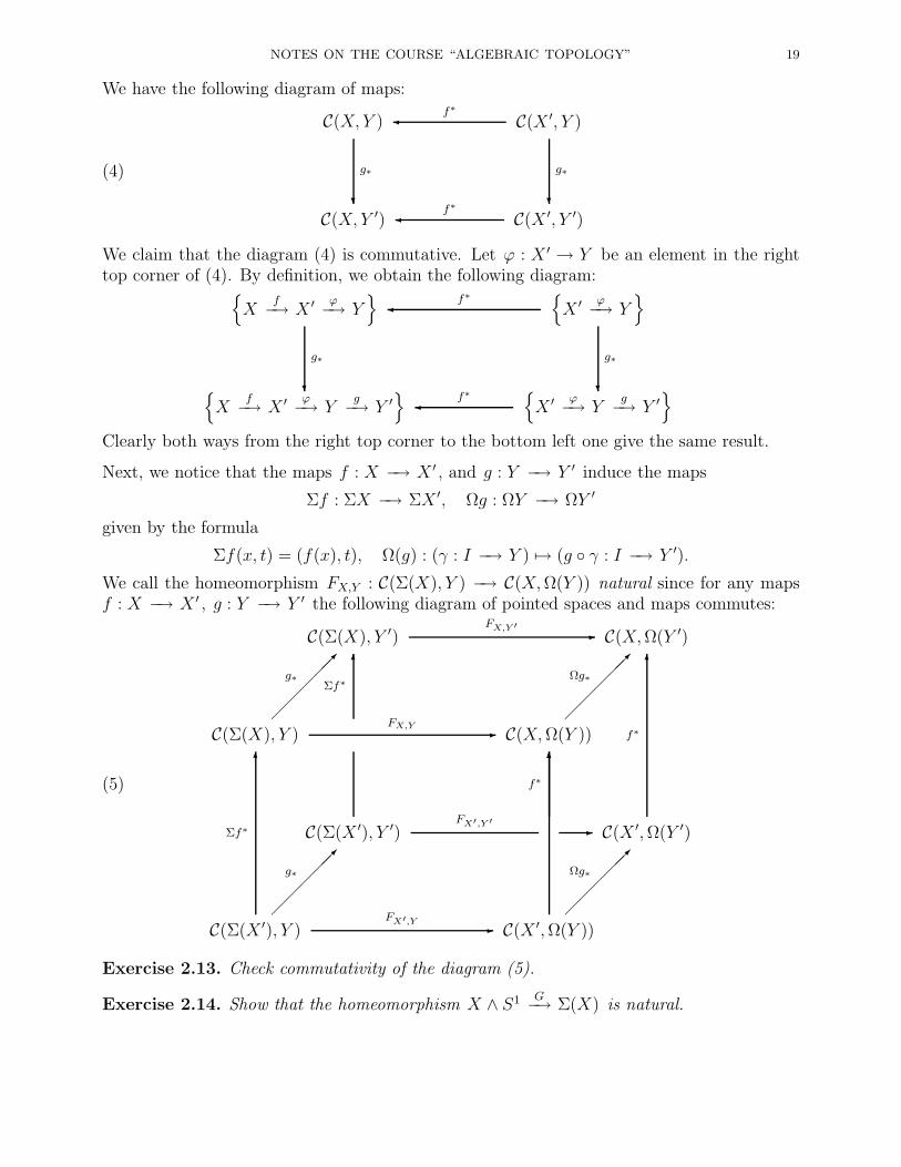
1. A one-point-union (or a bouquet) X ∨Y of pointed spaces (X, x0) and (Y, y0) is a disjointunion X ∪ Y with the points x0 and y0 identified, see Fig. 8.
Figure 8
2. A smash-product X ∧ Y is the factor-space: X ∧ Y = X × Y/((x0 × Y ) ∪ (X × y0)), seeFig. 9:
X ∧ Y :
X x0
y0
Y
Figure 9
Exercise 2.11. Prove that the space Sn ∧ Sn is homeomorphic to Sn+m as pointed spaces.
Exercise 2.12. Prove that X ∧ S1 is homeomorphic to Σ(X) as pointed spaces.
Remark. We have mentioned several natural homeomorphisms, for instance, the homeomor-phisms
(a) C(Σ(X), Y )FX,Y−−−→ C(X,Ω(Y )),
(b) X ∧ S1 G−→ Σ(X)
are natural. We would like to give more details.
First, let f : X −→ X ′ , and g : Y −→ Y ′ be maps of pointed spaces, then there the maps
f ∗ : C(X ′, Y ) −→ C(X, Y ),
g∗ : C(X, Y ) −→ C(X, Y ′),
given by the formula:
f ∗ : (ϕ : X ′ −→ Y ) 7→ (Xf−→ X ′ ϕ−→ Y ),
g∗ : (ψ : X −→ Y ) 7→ (Xψ−→ Y
g−→ Y ′).
NOTES ON THE COURSE “ALGEBRAIC TOPOLOGY” 19
We have the following diagram of maps:
(4)
C(X, Y )
?
g∗
C(X ′, Y )
?
g∗
f∗
C(X, Y ′) C(X ′, Y ′) f∗
We claim that the diagram (4) is commutative. Let ϕ : X ′ → Y be an element in the righttop corner of (4). By definition, we obtain the following diagram:
X
f−→ X ′ ϕ−→ Y
?
g∗
X ′ ϕ−→ Y
?
g∗
f∗
X
f−→ X ′ ϕ−→ Yg−→ Y ′
X ′ ϕ−→ Y
g−→ Y ′
f∗
Clearly both ways from the right top corner to the bottom left one give the same result.
Next, we notice that the maps f : X −→ X ′ , and g : Y −→ Y ′ induce the maps
Σf : ΣX −→ ΣX ′, Ωg : ΩY −→ ΩY ′
given by the formula
Σf(x, t) = (f(x), t), Ω(g) : (γ : I −→ Y ) 7→ (g γ : I −→ Y ′).
We call the homeomorphism FX,Y : C(Σ(X), Y ) −→ C(X,Ω(Y )) natural since for any mapsf : X −→ X ′ , g : Y −→ Y ′ the following diagram of pointed spaces and maps commutes:
(5)
C(Σ(X), Y ′) C(X,Ω(Y ′)-FX,Y ′
C(Σ(X), Y )
g∗6
Σf∗
C(X,Ω(Y ))
Ωg∗
-FX,Y
C(Σ(X ′), Y ′)
6f∗
C(X ′,Ω(Y ′)
6
f∗
FX′,Y ′
-
C(Σ(X ′), Y )
6
Σf∗
g∗
C(X ′,Ω(Y ))
Ωg∗
6
-FX′,Y
Exercise 2.13. Check commutativity of the diagram (5).
Exercise 2.14. Show that the homeomorphism X ∧ S1 G−→ Σ(X) is natural.

20 BORIS BOTVINNIK
3. Homotopy and homotopy equivalence
3.1. Definition of a homotopy. Let X and Y be topological spaces. Two maps
f0 : X −→ Y and f1 : X −→ Y
are homotopic (notation: f0 ∼ f1 ) if there exists a map F : X × I −→ Y such that therestriction F |X×0 coincides with f0 , and the restriction F |X×1 coincides with f1 .
The map F : X× I −→ Y is called a homotopy. We can think also that a homotopy betweenmaps f0 and f1 is a continuous family of maps ϕt : X −→ Y , 0 ≤ t ≤ 1, such that ϕ0 = f0 ,ϕ1 = f1 , and the map F : X × I −→ Y , F (x, t) = ϕt(x) is a continuous map for every t ∈ I .
If the spaces X and Y are “good spaces” (like our examples Sn , RPn , CPn , HPn , G(n, k)V (n, k) and so on), then we can think about homotopy between f0 and f1 as a path in thespace of continuous maps C(X, Y ) joining f0 and f1 . Furthemore, in such case, the set ofhomotopy classes [X, Y ] (see below) may be identified with the set of path-components ofthe space C(X, Y ).
If a map f : X −→ Y is homotopic to a constant map X −→ pt ∈ Y , we call the map fnull-homotopic.
Example. Let Y ⊂ Rn (or R∞ ) be a convex subset. Then for any space X any two mapsf0 : X −→ Y and f1 : X −→ Y are homotopic. Indeed, the map
F : x −→ (1− t)f0(x) + tf1(x)
defines a corresponding homotopy.
3.2. Homotopy classes of maps. Clearly a homotopy determines an equivalence relationon the space of maps C(X, Y ). The set of equivalence classes is denoted by [X, Y ] and it iscalled a set of homotopy classes.
Examples. 1. The set [X, ∗] consists of one point for any space X .
2. The space [∗, Y ] is the set of path-connected components of Y .
Let ϕ : X −→ X ′ be a map (continuous), then we define the map (not continuous since wedo not have a topology on the set [X, Y ]) ϕ∗ : [X ′, Y ] −→ [X, Y ] as follows. Let a ∈ [X ′, Y ]be a homotopy class. Choose any representative f : X ′ −→ Y of the class a, then ϕ∗(a) is ahomotopy class contaning the map f ϕ : X −→ Y .
Now let ψ : Y −→ Y ′ be a map. Then the map ψ∗ : [X, Y ] −→ [X, Y ′] is defined as follows.For any b ∈ [X, Y ] and a representative g : X −→ Y the map ψ g : X −→ Y ′ determines ahomotopy class ψ(b) = [ψ g].
Exercise 3.1. Prove that the maps ϕ∗ and ψ∗ are well-defined.
3.3. Homotopy equivalence. We will give three different definitions of homotopy equiva-lence.
NOTES ON THE COURSE “ALGEBRAIC TOPOLOGY” 21
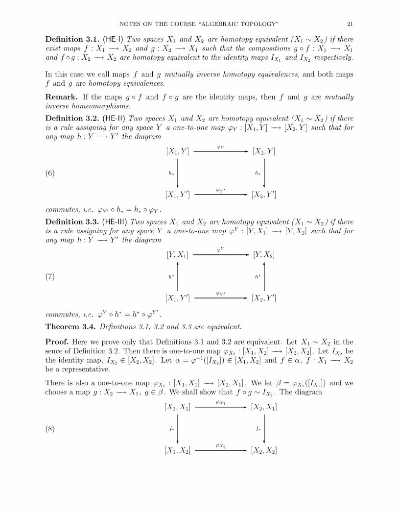
Definition 3.1. (HE-I) Two spaces X1 and X2 are homotopy equivalent (X1 ∼ X2 ) if thereexist maps f : X1 −→ X2 and g : X2 −→ X1 such that the compositions g f : X1 −→ X1
and f g : X2 −→ X2 are homotopy equivalent to the identity maps IX1 and IX2 respectively.
In this case we call maps f and g mutually inverse homotopy equivalences, and both mapsf and g are homotopy equivalences.
Remark. If the maps g f and f g are the identity maps, then f and g are mutuallyinverse homeomorphisms.
Definition 3.2. (HE-II) Two spaces X1 and X2 are homotopy equivalent (X1 ∼ X2 ) if thereis a rule assigning for any space Y a one-to-one map ϕY : [X1, Y ] −→ [X2, Y ] such that forany map h : Y −→ Y ′ the diagram
(6)
[X1, Y ]
?
h∗
[X2, Y ]
?
h∗
-ϕY
[X1, Y′] [X2, Y
′]-ϕY ′
commutes, i.e. ϕY ′ h∗ = h∗ ϕY .
Definition 3.3. (HE-III) Two spaces X1 and X2 are homotopy equivalent (X1 ∼ X2 ) if thereis a rule assigning for any space Y a one-to-one map ϕY : [Y,X1] −→ [Y,X2] such that forany map h : Y −→ Y ′ the diagram
(7)
[Y,X1] [Y,X2]-ϕY
[X1, Y′]
6
h∗
[X2, Y′]
6
h∗
-ϕY ′
commutes, i.e. ϕY h∗ = h∗ ϕY ′
.
Theorem 3.4. Definitions 3.1, 3.2 and 3.3 are equivalent.
Proof. Here we prove only that Definitions 3.1 and 3.2 are equivalent. Let X1 ∼ X2 in thesence of Definition 3.2. Then there is one-to-one map ϕX2 : [X1, X2] −→ [X2, X2]. Let IX2 bethe identity map, IX2 ∈ [X2, X2]. Let α = ϕ−1([IX2 ]) ∈ [X1, X2] and f ∈ α , f : X1 −→ X2
be a representative.
There is also a one-to-one map ϕX1 : [X1, X1] −→ [X2, X1]. We let β = ϕX1([IX1]) and wechoose a map g : X2 −→ X1 , g ∈ β . We shall show that f g ∼ IX2 . The diagram
(8)
[X1, X1]
?
f∗
[X2, X1]
?
f∗
-ϕX1
[X1, X2] [X2, X2]-ϕX2
22 BORIS BOTVINNIK
commutes by Definition 3.2. It implies that ϕX2 f∗ = f∗ ϕX1 . Let us consider the imageof the element [IX1] in the diagram (8). We have:
f∗([IX1 ] = [f IX1 ] = [f ], ϕX2([f ]) = [IX2]
by definition and by the choice of f . It implies that
ϕX2 f∗([IX1]) = [IX2 ].
On the other hand, we have:
f∗ ϕX1([IX1 ]) = f∗([g]) = [f g].Commutativity of (8) implies that [f g] = [IX2 ], i.e. f g ∼ IX2 .
A similar argument proves that gf ∼ IX1 . It means that X1 ∼ X2 in the sence of Definition3.1.
Now assume that X1 ∼ X2 in the sence of Definition 3.1, i.e. there are maps f : X1 −→ X2
and g : X1 −→ X1 such that f g ∼ IX2 and g f ∼ IX1 . Let Y be any space and define
ϕY = g∗ : [X1, Y ] −→ [X2, Y ].
We shall show that this map is inverse to the map
f ∗ : [X2, Y ] −→ [X1, Y ].
Indeed, let h ∈ C(X1, Y ), then
f ∗ g∗([h]) = f ∗([h g]) = (by definition of f ∗ ) = [h (g f)] = [h] (since g f ∼ IX1 ).
This shows that f ∗ is inverse to g∗ . With a similar argument we prove that g∗ is inverse tof ∗ . Thus ϕY = g∗ is a bijection. Now we have to check naturality.
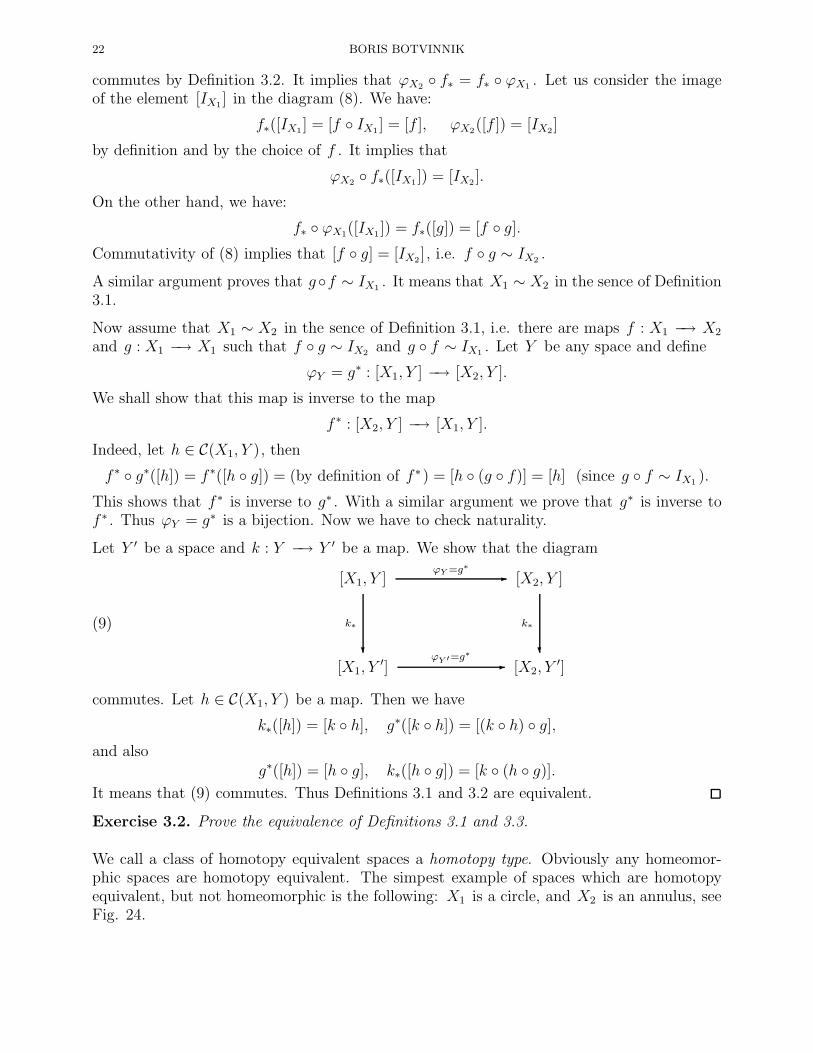
Let Y ′ be a space and k : Y −→ Y ′ be a map. We show that the diagram
(9)
[X1, Y ]
?
k∗
[X2, Y ]
?
k∗
-ϕY =g∗
[X1, Y′] [X2, Y
′]-ϕY ′=g∗
commutes. Let h ∈ C(X1, Y ) be a map. Then we have
k∗([h]) = [k h], g∗([k h]) = [(k h) g],and also
g∗([h]) = [h g], k∗([h g]) = [k (h g)].It means that (9) commutes. Thus Definitions 3.1 and 3.2 are equivalent.
Exercise 3.2. Prove the equivalence of Definitions 3.1 and 3.3.
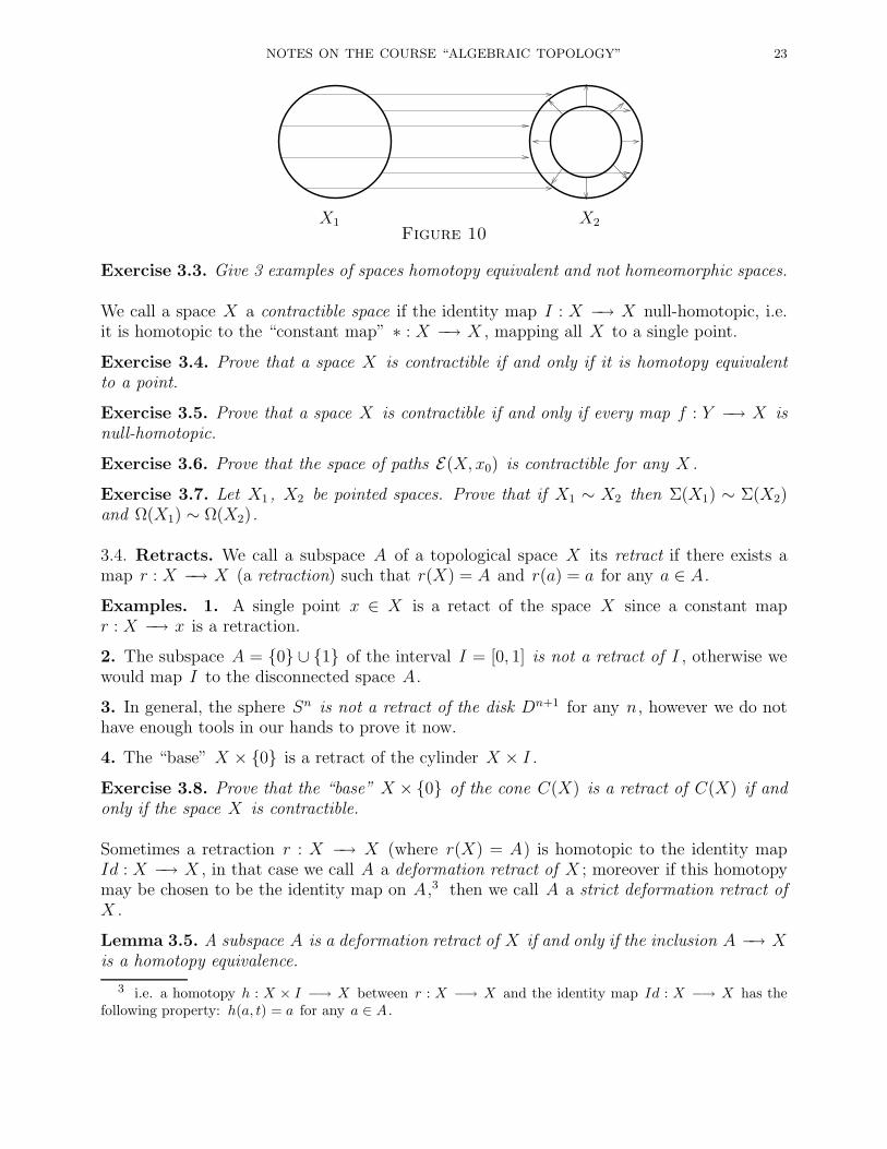
We call a class of homotopy equivalent spaces a homotopy type. Obviously any homeomor-phic spaces are homotopy equivalent. The simpest example of spaces which are homotopyequivalent, but not homeomorphic is the following: X1 is a circle, and X2 is an annulus, seeFig. 24.
NOTES ON THE COURSE “ALGEBRAIC TOPOLOGY” 23
X1 X2Figure 10
Exercise 3.3. Give 3 examples of spaces homotopy equivalent and not homeomorphic spaces.
We call a space X a contractible space if the identity map I : X −→ X null-homotopic, i.e.it is homotopic to the “constant map” ∗ : X −→ X , mapping all X to a single point.
Exercise 3.4. Prove that a space X is contractible if and only if it is homotopy equivalentto a point.
Exercise 3.5. Prove that a space X is contractible if and only if every map f : Y −→ X isnull-homotopic.
Exercise 3.6. Prove that the space of paths E(X, x0) is contractible for any X .
Exercise 3.7. Let X1 , X2 be pointed spaces. Prove that if X1 ∼ X2 then Σ(X1) ∼ Σ(X2)and Ω(X1) ∼ Ω(X2).
3.4. Retracts. We call a subspace A of a topological space X its retract if there exists amap r : X −→ X (a retraction) such that r(X) = A and r(a) = a for any a ∈ A.
Examples. 1. A single point x ∈ X is a retact of the space X since a constant mapr : X −→ x is a retraction.
2. The subspace A = 0 ∪ 1 of the interval I = [0, 1] is not a retract of I , otherwise wewould map I to the disconnected space A.
3. In general, the sphere Sn is not a retract of the disk Dn+1 for any n, however we do nothave enough tools in our hands to prove it now.
4. The “base” X × 0 is a retract of the cylinder X × I .
Exercise 3.8. Prove that the “base” X × 0 of the cone C(X) is a retract of C(X) if andonly if the space X is contractible.
Sometimes a retraction r : X −→ X (where r(X) = A) is homotopic to the identity mapId : X −→ X , in that case we call A a deformation retract of X ; moreover if this homotopymay be chosen to be the identity map on A,3 then we call A a strict deformation retract ofX .
Lemma 3.5. A subspace A is a deformation retract of X if and only if the inclusion A −→ Xis a homotopy equivalence.
3 i.e. a homotopy h : X × I −→ X between r : X −→ X and the identity map Id : X −→ X has thefollowing property: h(a, t) = a for any a ∈ A .

24 BORIS BOTVINNIK
Exercise 3.9. Prove Lemma 3.5.
Lemma 3.5 shows that a concept of deformation retract is not really new for us; a concept ofstrict deformation retract is more restrictive, however these two concepts are different only insome pathological cases.
Exercise 3.10. Let A ⊂ X , and r(0) : X −→ A, r(1) : X −→ A be two deformationretractions. Prove that the retractions r(0) , r(1) may be joined by a continuous family ofdeformation retractions r(s) : X −→ A, 0 ≤ s ≤ 1. Note: It is important here that r(0) , r(1)
are both homotopic to the identity map IX .
3.5. The case of “pointed” spaces. The definitions of homotopy, homotopy equivalencehave to be changed (in an obvious way) for spaces with base points. The set of homotopyclases of “pointed” maps f : X −→ Y will be also denoted as [X, Y ]. We need one moregeneralization.
Definition 3.6. A pair (X,A) is just a space X with a labeled subspace A ⊂ X ; a mapof pairs f : (X,A) −→ (Y,B) is a continuous map f : X −→ Y such that f(A) ⊂ B .Two maps (X,A) −→ (Y,B), f1 : (X,A) −→ (Y,B) are homotopic if there exist a mapF : (X × I, A× I) −→ (Y,B) such that
F |(X×0,A×0 = f0, F |(X×1,A×1 = f1.
We have seen already the example of pairs and their maps. Let me recall that the cones ofthe maps c : Sn −→ RPn and h : S2n+1 −→ CPn give us the commutative diagrams:
(10)
Dn+1 RPn+1 D2n+2 CPn+1-f -g
Sn
6
i
RPn
6
i
S2n+1
6
i
CPn
6
i
-c -h
which are the maps of pairs:
f : (Dn+1, Sn) −→ (RPn+1,RPn), g : (D2n+2, S2n+1) −→ (CPn+1,CPn).
NOTES ON THE COURSE “ALGEBRAIC TOPOLOGY” 25
4. CW -complexes
Algebraic topologists rarely study arbitrary topological spaces: there is not much one canprove about an abstract topological space. However, there is very well-developed area knownas general topology which studies simple properties (such as conectivity, the Hausdorff prop-erty, compactness and so on) of complicated spaces. There is a giant Zoo out there of verycomplicated spaces endowed with all possible degrees of pathology, i.e. when one or anothersimple property fails or holds. Some of these spaces are extremely useful, such as the Cantorset or fractals, they help us to understand very delicate phenomenas observed in mathematicsand physics. In algebraic topology we mostly study complicated properties of simple spaces.
It turns out that the most important spaces which are important for mathematics have someadditional structures. The first algebraic topologist, Poincare, studied mostly the spacesendowed with “analytic” structures, i.e. when a space X has natural differential structureor Riemannian metric and so on. The major advantage of these structures is that they allare natural, so we should not really care about their existence: they are given! There is theother type of natural structures on topological spaces: so called combinatorial structures, i.e.when a space X comes equipped with a decomposition into more or less “standard pieces”, sothat one could study the whole space X by examination the mutual geometric and algebraicrelations between those “standard pieces”. Below we formalize this concept: these spaces areknown as CW -complexes. For instance, all examples we studied so far are like that.
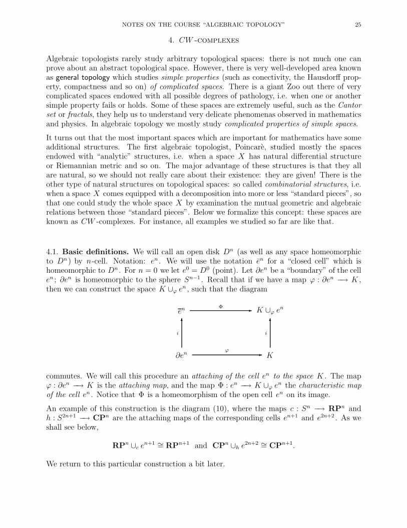
4.1. Basic definitions. We will call an open disk Dn (as well as any space homeomorphicto Dn ) by n-cell. Notation: en . We will use the notation en for a “closed cell” which ishomeomorphic to Dn . For n = 0 we let e0 = D0 (point). Let ∂en be a “boundary” of the cellen ; ∂en is homeomorphic to the sphere Sn−1 . Recall that if we have a map ϕ : ∂en −→ K ,then we can construct the space K ∪ϕ en , such that the diagram
en K ∪ϕ en-Φ
∂en
6
i
K
6
i
-ϕ
commutes. We will call this procedure an attaching of the cell en to the space K . The mapϕ : ∂en −→ K is the attaching map, and the map Φ : en −→ K ∪ϕ en the characteristic mapof the cell en . Notice that Φ is a homeomorphism of the open cell en on its image.
An example of this construction is the diagram (10), where the maps c : Sn −→ RPn andh : S2n+1 −→ CPn are the attaching maps of the corresponding cells en+1 and e2n+2 . As weshall see below,
RPn ∪c en+1 ∼= RPn+1 and CPn ∪h e2n+2 ∼= CPn+1.
We return to this particular construction a bit later.
26 BORIS BOTVINNIK
Definition 4.1. A Hausdorff topological space X is a CW -complex (or cell-complex) if it isdecomposed as a union of cells:
X =
∞⋃
q=0
⋃
i∈Iqeqi
,
where the cells eqi ∩ epj = ∅ unless q = p, i = j , and for each eqi there exists a characteristic
map Φ : Dq −→ X such that its restriction Φ
Dq gives a homeomorphism Φ|
Dq :
Dq
−→ eqi .
It is required that the following axioms are satisfied:
(C) (close finite) The boundary ∂eqi = eqi \ eqi of the cell eqi is a subset of the union of finitenumber of cells erj , where r < q .
(W) (weak topology) A set F ⊂ X is closed if and only if the intersection F ∩ en is closedfor every cell eqi .
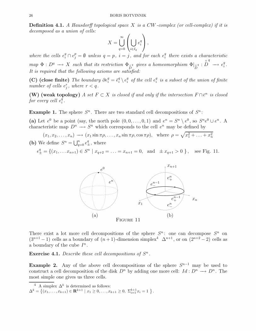
Example 1. The sphere Sn . There are two standard cell decompositions of Sn :
(a) Let e0 be a point (say, the north pole (0, 0, . . . , 0, 1) and en = Sn \ e0 , so Sne0 ∪ en . Acharacteristic map Dn −→ Sn which corresponds to the cell en may be defined by
(x1, x2, . . . , xn) −→ (x1 sin πρ, . . . , xn sin πρ, cosπρ), where ρ =√x2
1 + . . .+ x2n
(b) We define Sn =⋃nq=0 e
q± , where
eq± = (x1, . . . xn+1) ∈ Sn | xq+2 = . . . = xn+1 = 0, and ± xq+1 > 0 , see Fig. 11.
(a) (b)
e0
en
x1
xn
xn+1
en+
en−
en−1+
en−1−
Figure 11
There exist a lot more cell decompositions of the sphere Sn : one can decompose Sn on(3n+1− 1) cells as a boundary of (n+ 1)-dimension simplex4 ∆n+1 , or on (2n+2− 2) cells asa boundary of the cube In .
Exercise 4.1. Describe these cell decompositions of Sn .
Example 2. Any of the above cell decompositions of the sphere Sn−1 may be used toconstruct a cell decomposition of the disk Dn by adding one more cell: Id : Dn −→ Dn . Themost simple one gives us three cells.
4 A simplex ∆k is determined as follows:∆k =
(x1, . . . , xk+1) ∈ Rk+1 | x1 ≥ 0, . . . , xk+1 ≥ 0, Σk+1
i=1xi = 1
.

NOTES ON THE COURSE “ALGEBRAIC TOPOLOGY” 27
4.2. Some comments on the definition of a CW -complex. 1o Let X be a CW-complex.We denote X(n) the union of all cells in X of dimension ≤ n. This is the n-th skeleton ofX . The n-th skeleton X(n) is an example (very important one) of a subcomplex of a CW -complex. A subcomplex A ⊂ X is a closed subset of A which is a union of some cells ofX . In particular, the n-th skeleton A(n) is a subcomplex of X(n) for each n ≥ 0. A mapf : X −→ Y of CW -complexes is a cellular map if f |X(n) maps the n-th skeleton to then-skeleton Y (n) for each n ≥ 0. In particular, the inclusion A ⊂ X of a subcomplex is acellular map. A CW -complex is called finite if it has a finite number of cells. A CW -complexis called locally finite if X has a finite number of cells in each dimension. Finally (X, x0) isa pointed CW -complex, if x0 is a 0-cell.
Exercise 4.2. Prove that a CW -complex compact if and only if it is finite.
2o It turns out that a closure of a cell within a CW -complex may be not a CW -complex.
Exercise 4.3. Construct a cellular decomposion of the wedge X = S1 ∨ S2 (with a single2-cell e2 ) such that a closure of the cell e2 is not a CW -subcomplex of X .
3o (Warning) The axiom (W ) does not imply the axiom (C). Indeed, consider a decom-position of the disk D2 into 2-cell e2 which is the interior of the disk D2 and each point ofthe circle S1 is considered as a zero cell.
Exercise 4.4. Prove that the disk D2 with the cellular decomposition described above satisfies(W ), and does not satisfy (C).
Figure 12
4o (Warning) The axiom (C) does not imply the axiom (W ). Indeed, consider the followingspace X . We start with an infinite (even countable) family Iα of unit intervals. Let X =∨α Iα , where we identify zero points of all intervals Iα . We define a topology on X by means
of the following metric. Let t′ ∈ Iα′ and t′′ ∈ Iα′′ . Then a distance is defined by
ρ(t′, t′′) =
|t′ − t′′| if α′ = α′′
t′ + t′′ if α′ 6= α′′
Exercise 4.5. Check that a natural cellular decomposition of X into the interiors of Iα andremaining points (zero cells) does not satisfy the axiom (W ).
4.3. Operations on CW -complexes. All operations we considered are well-defined on thecategory of CW -complexes, however we have to be a bit careful. If one of the CW -complexesX and Y is locally finite, then the product X×Y has a canonical CW -structure. The sameholds for a smash-product X ∧ Y of pointed CW -complexes. The cone C(X), cylinder
28 BORIS BOTVINNIK
X × I , and suspension Σ(X) has canonical CW -structure determined by X . We can glueCW -complexes X ∪f Y if f : A −→ Y a cellular map, and A ⊂ X is a subcomplex. Also thequotient space X/A is a CW -complex if (A,X) is a CW -pair. The functional spaces C(X, Y )are two big to have natural CW -structure, however, a space C(X, Y ) is homotopy equivalentto a CW -complex if X and Y are CW -complexes. The last statement is a nontrivial resultdue to J. Milnor (1958).
4.4. More examples of CW -complexes. Real projective space RPn . Here we choose inRPn a sequence of projective subspaces:
∗ = RP0 ⊂ RP1 ⊂ . . . ⊂ RPn−1 ⊂ RPn.
and set e0 = RP0 , e1 = RP1 \RP0, . . . en = RPn \RPn−1 . The diagram (10) shows thatthe map c : Sk−1 −→ RPk is an attaching map, and its extension to the cone over Sk−1
(the disk Dk ) is a characteristic map of the cell ek . Alternatively this decomposition may bedescribed in the homogeneous coordinates as follows. Let
eq = (x0 : x1 : · · · : xn) | xq 6= 0, xq+1 = 0, . . . xn = 0 .Exercise 4.6. Prove that eq is homeomorphic to RPq \RPq−1 .
Exercise 4.7. Construct cell decompositions of CPn and HPn .
Exercise 4.8. Represent as CW -complex every 2-dimensional manifold. Try to find a CW -strucute with a minimal number of cells.
Exercise 4.9. Prove that a finite CW -complex (with finite number of cells) may be embeddedinto Euclidean space of finite dimension.
4.5. CW -structure of the Grassmanian manifolds. We describe here the Schubert de-composition, and the cells of this decomposition are known as the Schubert cells. We considerthe space G(n, k). We choose the standard basis e1, . . . , en of Rn . Let Rq = 〈e1, . . . , eq〉 . Itis convenient to denote R0 = 0 . We have the inclusions:
R0 ⊂ R1 ⊂ R2 ⊂ · · · ⊂ Rn.
Let π ∈ G(n, k). Clearly π determines a collection of nonnegative numbers
0 ≤ dim(R1 ∩ π) ≤ dim(R2 ∩ π) ≤ · · · ≤ dim(Rn ∩ π) = k.
We note that dim(Rj ∩ π) ≤ dim(Rj−1 ∩ π) + 1. Indeed, we have linear maps
(11) 0 −→ Rj−1 ∩ π i−→ Rj ∩ π j -th coordinate−−−−−−−−−−−→ R
where the first one, i : Rj−1 ∩ π −→ Rj ∩ π , is an embedding, and the map
j -th coordinate : Rj ∩ π −→ R
is either onto or zero. In the first case dim(Rj ∩ π) = dim(Rj−1 ∩ π) + 1, and in the secondcase dim(Rj ∩ π) = dim(Rj−1 ∩ π). Thus there are exactly k “jumps” in the sequence(0, dim(R1 ∩ π), . . . , dim(Rn ∩ π)).
A Schubert symbol σ = (σ1, . . . , σn) is a collection of integers, such that
1 ≤ σ1 < σ2 < · · · < σk ≤ n.
NOTES ON THE COURSE “ALGEBRAIC TOPOLOGY” 29
Let e(σ) ⊂ G(n, k) be the following set of the following k -planes in Rn
e(σ) =π ∈ G(n, k) | dim(Rσj ∩ π) = j & dim(Rσj−1 ∩ π) = j − 1, j = 1, . . . , k
.
Notice that every π ∈ G(n, k) belongs to exactly one subset e(σ). Indeed, in the sequence ofsubspaces
R1 ∩ π ⊂ R2 ∩ π ⊂ · · · ⊂ Rn ∩ π = π
their dimensions “jump” by one exactly k times. Clearly π ∈ e(σ), where σ = (σ1, . . . , σn)and
σt = minj | dim(Rj ∩ π) = t
.
Our goal is to prove that the set e(σ) is homeomorphic to an open cell of dimension d(σ) =(σ1 − 1) + (σ2 − 2) + · · ·+ (σk − k). Let Hj ⊂ Rn denote an open “half j -plane of Rj :
Hj = (x1, . . . , xj, 0, . . . , 0) | xj > 0 .It will be convenient to denote H
j= (x1, . . . , xj , 0, . . . , 0) | xj ≥ 0 .
Claim 4.1. A k -plane π belongs to e(σ) if and only if there exists its basis v1, . . . , vk , suchthat v1 ∈ Hσ1 , . . ., vk ∈ Hσk .
Proof. Indeed, if there is such a basis v1, . . . , vk then
dim(Rσj ∩ π) > dim(Rσj−1 ∩ π)
for j = 1, . . . , k . Thus π ∈ e(σ). The following lemma proves Claim 4.1 in the other direction.
Lemma 4.2. Let π ∈ e(σ), where σ = (σ1, . . . , σn). Then there exists a unique orthonormalbasis v1, . . . , vk of π , so that v1 ∈ Hσ1 , . . ., vk ∈ Hσk .
Proof. We choose v1 to be a unit vector which generates the line Rσ1∩π . There are only twochoices here, and the condition that the σ1 -th coordinate is positive determines v1 uniquely.Then the unit vector v2 ∈ Rσ2∩π should be chosen so that v2 ⊥ v1 . There are two choices likethat, and again the positivity of the σ2 -th coordinate determines v2 uniquely. By inductionone obtains the required basis. This completes proof of Lemma 4.2 and Claim 4.1.
We define the following subset of the Stiefel manifold V (n, k):
E(σ) = (v1, . . . , vk) ∈ V (n, k) | v1 ∈ Hσ1 , . . . , vk ∈ Hσk .Lemma 4.2 gives a well-defined map q : e(σ) −→ E(σ). It is convenient to denote E(σ) =(v1, . . . , vk) ∈ V (n, k) | v1 ∈ H
σ1, . . . , vk ∈ H
σk
.
Claim 4.2. The set E(σ) ⊂ V (n, k) is homeomorphic to the closed cell of dimension d(σ) =(σ1−1)+(σ2−2)+· · ·+(σk−k). Furthermore the map q : e(σ) −→ E(σ) is a homeomorphism.
Proof. Induction on k . If k = 1 the set E(σ1) consists of the vectors
v1 = (x11, . . . , x1σ1 , 0, . . . , 0), such that∑
x21j = 1, and x1σ1 ≥ 0.
Clearly E(σ1) is a closed hemisphere of dimension (σ1 − 1), i.e. E(σ1) is homeomorphic tothe disk Dσ1−1 .
To make an induction step, consider the following construction. Let u, v ∈ Rn be two unitvectors such that u 6= −v . Let Tu,v an orthogonal transformation Rn −→ Rn such that
30 BORIS BOTVINNIK
(1) Tu,v(u) = v ;(2) Tu,v(w) = w if w ∈ 〈u, v〉⊥ .
In other words, Tu,v is a rotation in the plane 〈u, v〉 taking the vector u to v , and is identityon the orthogonal complement to the plane 〈u, v〉 generated by u and v .
Claim 4.3. The transformation Tu,v (where u, v ∈ Rn , u 6= −v) has the following properties:
(a) Tu,u = Id;(b) Tv,u = T−1
u,v ;(c) Tv,u : Rn −→ Rn is be given by
Tu,v(x) = x− 〈u+ v, x〉1 + 〈u, v〉 (u+ v) + 2〈u, x〉v;
(d) a vector Tu,v(x) depends continuously on u, v, x;(e) Tu,v(x) = x (mod Rj ) if u, v ∈ Rj .
The properties (a), (b), (e) follow from the definition.
Exercise 4.10. Prove (c), (d) from Claim 4.3.
Let ǫi ∈ Hσi be a vector which has σi -coordinate equal to 1, and all others are zeros. Thus(ǫ1, . . . , ǫk) ∈ E(σ). For each k -frame (v1, . . . , vk) ∈ E(σ) consider the transformation:
(12) T = Tǫk,vk Tǫk−1,vk−1
· · · · · · Tǫ1,v1 : Rn −→ Rn
First we notice that vi 6= −ǫi since vi ∈ Hσi
. Thus the transformations Tǫi,viare well-defined.
Exercise 4.11. Prove that the transformation T takes the k -frame (ǫ1, . . . , ǫk) to the frame(v1, . . . , vk).
Consider the following subspace D ⊂ Hσk+1
:
D =u ∈ Hσk+1 | |u| = 1, 〈ǫj, u〉 = 0, j = 1, . . . , k
.
Exercise 4.12. Prove that D is homeomorphic to the hemisphere of the dimension σk+1 −k − 1.
Thus D is a closed cell of dimension σk+1−k−1. Now we make an induction step to completea proof of Claim 4.2. We define the map
f : E(σ1, . . . , σk)×D −→ E(σ1, . . . , σk, σk+1)
by the formula f((v1, . . . , vk), u) = (v1, . . . , vk, Tu) where T is given by (12). We notice that
〈vi, Tu〉 = 〈Tǫi, Tu〉 = 〈ǫi, u〉 = 0, i = 1, . . . , k,
and 〈Tu, Tu〉 = 〈u, u〉 = 1 by definition of T and since T ∈ O(n).
Exercise 4.13. Recall that σk < σk+1 . Prove that Tu ∈ Hσk+1 if u ∈ D .
NOTES ON THE COURSE “ALGEBRAIC TOPOLOGY” 31
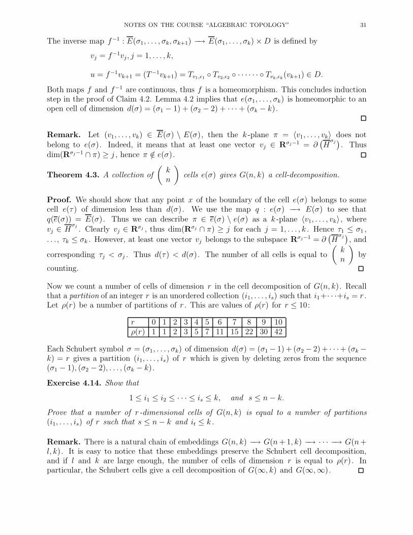
The inverse map f−1 : E(σ1, . . . , σk, σk+1) −→ E(σ1, . . . , σk)×D is defined by
vj = f−1vj , j = 1, . . . , k,
u = f−1vk+1 = (T−1vk+1) = Tv1,ǫ1 Tv2,ǫ2 · · · · · · Tvk,ǫk(vk+1) ∈ D.Both maps f and f−1 are continuous, thus f is a homeomorphism. This concludes inductionstep in the proof of Claim 4.2. Lemma 4.2 implies that e(σ1, . . . , σk) is homeomorphic to anopen cell of dimension d(σ) = (σ1 − 1) + (σ2 − 2) + · · ·+ (σk − k).
Remark. Let (v1, . . . , vk) ∈ E(σ) \ E(σ), then the k -plane π = 〈v1, . . . , vk〉 does notbelong to e(σ). Indeed, it means that at least one vector vj ∈ Rσj−1 = ∂
(Hσj). Thus
dim(Rσj−1 ∩ π) ≥ j , hence π /∈ e(σ).
Theorem 4.3. A collection of
(kn
)cells e(σ) gives G(n, k) a cell-decomposition.
Proof. We should show that any point x of the boundary of the cell e(σ) belongs to somecell e(τ) of dimension less than d(σ). We use the map q : e(σ) −→ E(σ) to see thatq(e(σ)) = E(σ). Thus we can describe π ∈ e(σ) \ e(σ) as a k -plane 〈v1, . . . , vk〉 , wherevj ∈ H
σj. Clearly vj ∈ Rσj , thus dim(Rσj ∩ π) ≥ j for each j = 1, . . . , k . Hence τ1 ≤ σ1 ,
. . ., τk ≤ σk . However, at least one vector vj belongs to the subspace Rσj−1 = ∂(Hσj), and
corresponding τj < σj . Thus d(τ) < d(σ). The number of all cells is equal to
(kn
)by
counting.
Now we count a number of cells of dimension r in the cell decomposition of G(n, k). Recallthat a partition of an integer r is an unordered collection (i1, . . . , is) such that i1+· · ·+is = r .Let ρ(r) be a number of partitions of r . This are values of ρ(r) for r ≤ 10:
r 0 1 2 3 4 5 6 7 8 9 10ρ(r) 1 1 2 3 5 7 11 15 22 30 42
Each Schubert symbol σ = (σ1, . . . , σk) of dimension d(σ) = (σ1− 1) + (σ2− 2) + · · ·+ (σk −k) = r gives a partition (i1, . . . , is) of r which is given by deleting zeros from the sequence(σ1 − 1), (σ2 − 2), . . . , (σk − k).Exercise 4.14. Show that
1 ≤ i1 ≤ i2 ≤ · · · ≤ is ≤ k, and s ≤ n− k.Prove that a number of r -dimensional cells of G(n, k) is equal to a number of partitions(i1, . . . , is) of r such that s ≤ n− k and it ≤ k .
Remark. There is a natural chain of embeddings G(n, k) −→ G(n+ 1, k) −→ · · · −→ G(n+l, k). It is easy to notice that these embeddings preserve the Schubert cell decomposition,and if l and k are large enough, the number of cells of dimension r is equal to ρ(r). Inparticular, the Schubert cells give a cell decomposition of G(∞, k) and G(∞,∞).
32 BORIS BOTVINNIK
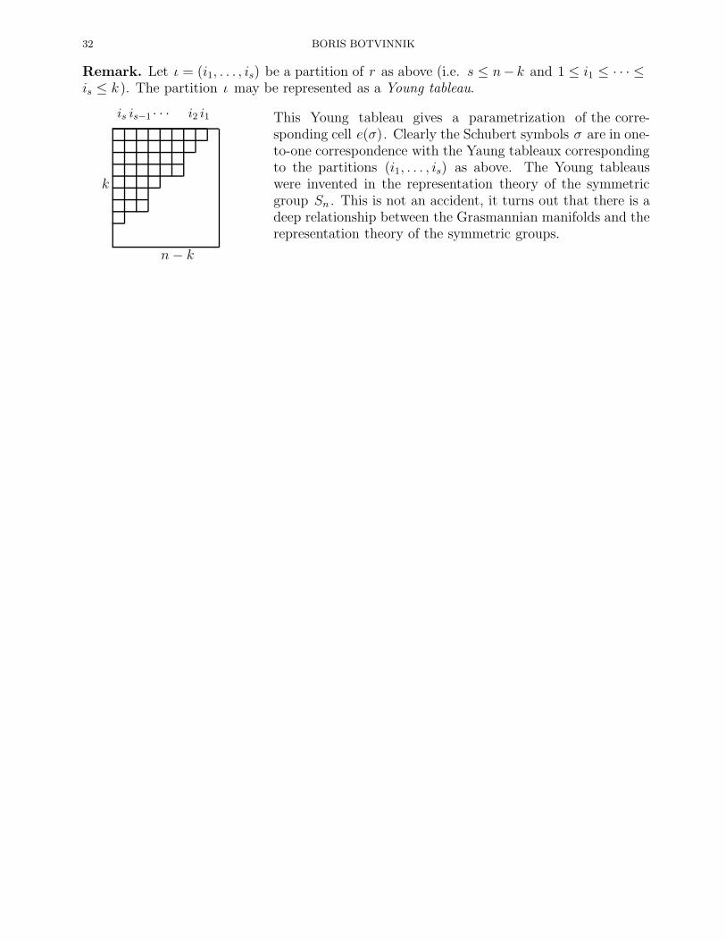
Remark. Let ι = (i1, . . . , is) be a partition of r as above (i.e. s ≤ n− k and 1 ≤ i1 ≤ · · · ≤is ≤ k ). The partition ι may be represented as a Young tableau.
is is−1 · · · i2 i1
n− k
k
This Young tableau gives a parametrization of the corre-sponding cell e(σ). Clearly the Schubert symbols σ are in one-to-one correspondence with the Yaung tableaux correspondingto the partitions (i1, . . . , is) as above. The Young tableauswere invented in the representation theory of the symmetricgroup Sn . This is not an accident, it turns out that there is adeep relationship between the Grasmannian manifolds and therepresentation theory of the symmetric groups.
NOTES ON THE COURSE “ALGEBRAIC TOPOLOGY” 33
5. CW -complexes and homotopy
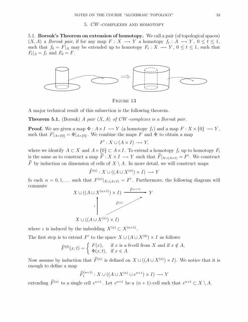
5.1. Borsuk’s Theorem on extension of homotopy. We call a pair (of topological spaces)(X,A) a Borsuk pair, if for any map F : X −→ Y a homotopy ft : A −→ Y , 0 ≤ t ≤ 1,such that f0 = F |A may be extended up to homotopy Ft : X −→ Y , 0 ≤ t ≤ 1, such thatFt|A = ft and F0 = F .
Figure 13
A major technical result of this subsection is the following theorem.
Theorem 5.1. (Borsuk) A pair (X,A) of CW -complexes is a Borsuk pair.
Proof. We are given a map Φ : A×I −→ Y (a homotopy ft ) and a map F : X×0 −→ Y ,such that F |A×0 = Φ|A×0 . We combine the maps F and Φ to obtain a map
F ′ : X ∪ (A× I) −→ Y,
where we identify A ⊂ X and A×0 ⊂ A×I . To extend a homotopy ft up to homotopy Ftis the same as to construct a map F : X × I −→ Y such that F |X∪(A×I) = F ′ . We construct
F by induction on dimension of cells of X \ A. In more detail, we will construct maps
F (n) : X ∪ ((A ∪X(n))× I) −→ Y
fo each n = 0, 1, . . . such that F (n)|X∪(A×I) = F ′ . Furthermore, the following diagram willcommute
X ∪ ((A ∪X(n+1))× I) Y-bF (n+1)
X ∪ ((A ∪X(n))× I)
6ι
*bF (n)
where ι is induced by the imbedding X(n) ⊂ X(n+1) .
The first step is to extend F ′ to the space X ∪ (A ∪X(0))× I as follows:
F (0)(x, t) =
F (x), if x is a 0-cell from X and if x /∈ A,Φ(x, t), if x ∈ A.
Now assume by induction that F (n) is defined on X ∪ ((A ∪X(n))× I). We notice that it isenough to define a map
F(n+1)1 : X ∪ ((A ∪X(n) ∪ en+1)× I) −→ Y
extending F (n) to a single cell en+1 . Let en+1 be a (n+ 1)-cell such that en+1 ⊂ X \ A.

34 BORIS BOTVINNIK
By induction, the map F (n) is already given on the cylinder (en+1\en+1)×I since the boundary∂en+1 = en+1 \ en+1 ⊂ X(n) . Let g : Dn+1 −→ X(n+1) be a characteristic map corresponding
to the cell en+1 . We have to define an extension of F(n)1 from the side g(Sn) × I and the
bottom base g(Dn+1)×0 to the cylinder g(Dn+1)× I . By definition of CW -complex, it isthe same as to construct an extension of the map
ψ = F (n) g : (Dn+1 × 0) ∪ (Sn × I) −→ Y
to a map of the cylinder ψ′ : Dn+1 × I −→ Y . Let
η : Dn+1 × I −→ (Dn+1 × 0) ∪ (Sn × I)be a projection map of the cylinder Dn+1 × I from a point s which is near and a bit aboveof the top side Dn+1 × 1 of the cylinder Dn+1 × I , see the Figure below.
The map η is an identical map on (Dn+1×0)∪ (Sn× I). Wedefine an extension ψ′ as follows:
ψ′ : Dn+1 × I η−→ (Dn+1 × 0) ∪ (Sn × I) ψ−→ Y.
This procedure may be carried out independently for all (n+1)-cells of X , so we obtain an extension
F (n+1) : X ∪ ((A ∪X(n+1))× I) −→ Y.
Exercise 5.1. Let Dn+1 × I ⊂ Rn+1 given by:
Dn+1 × I =(x1, . . . , xn+1, xn+2) | x2
1 + · · ·+ x2n+1 ≤ 1, xn+2 ∈ [0, 1]
.
Give a formula for the above map η .
Thus, going from the skeleton X(n) to the skeleton X(n+1) , we construct an extension F :X × I −→ Y of the map F ′ : X ∪ (A× I) −→ Y .
We should emphasize that if X is an infinite-dimensional complex, then our construction
consists of infinite number of steps; in that case the axiom (W) implies that F is a continuousmap.
Corollary 5.2. Let X be a CW -complex and A ⊂ X be its contractible subcomplex. ThenX is homotopy equivalent to the complex X/A.
Proof. Let p : X −→ X/A be a projection map. Since A is a contractible there exists ahomotopy ft : A −→ A such that f0 : A −→ A is an identity map, and f1(A) = x0 ∈ A. ByTheorem 5.1 there exists a homotopy Ft : X −→ X , 0 ≤ t ≤ 1, such that F0 = IdX andFt|A = ft . In particular, F1(A) = x0 . It means that F1 may be considered as a map givenon X/A, (by definition of the quotient topology), i.e.
F1 = q p : Xp−→ X/A
q−→ X,
where q : X/A −→ X is some continuous map. By construction, F1 ∼ F0 , i.e. q p ∼ IdX .
Now, Ft(A) ⊂ A for any t, i.e. p Ft(A) = x0 . It follows that p Ft = ht p, whereht : X/A −→ X/A is some homotopy, such that h0 = IdX/A and h1 = p q ; it means thatp q ∼ IdX/A .
NOTES ON THE COURSE “ALGEBRAIC TOPOLOGY” 35
Corollary 5.3. Let X be a CW -complex and A ⊂ X be its subcomplex. Then X/A ishomotopy equivalent to the complex X ∪ C(A), where C(A) is a cone over A.
Exercise 5.2. Prove Corollary 5.3.
5.2. Cellular Approximation Theorem. Let X and Y be CW -complexes. Recall that amap f : X −→ Y is a cellular map if f(X(n)) ⊂ Y (n) for every n = 0, 1, . . .. We emphasizethat it is not required that the image of n-cell belongs to a union of n-cells. For example, aconstant map ∗ : X −→ x0 = e0 is a cell map. The following theorem provides very importanttool in algebraic topology.
Theorem 5.4. Any continuous map f : X −→ Y of CW -complexes is homotopic to acellular map.
We shall prove the following stronger statement:
Theorem 5.5. Let f : X −→ Y be a continuous map of CW -complexes, such that a re-striction f |A is a cellular map on a CW -subcomplex A ⊂ X . Then there exists a cell mapg : X −→ Y such that g|A = f |A and, moreover, f ∼ g rel A.
First of all, we should explain the notation f ∼ g rel A which we are using. Assume that weare given two maps f, g : X −→ Y such that f |A = g|A . A notation f ∼ g rel A means thatthere exists a homotopy ht : X −→ Y such that ht(a) does not depend on t for any a ∈ A.Certainly f ∼ g rel A implies f ∼ g , but f ∼ g does not imply f ∼ g rel A.
Exercise 5.3. Give an example of a map f : [0, 1] −→ S1 which is homotopic to a constantmap, and, at the same time f is not homotopic to a constant map relatively to A = 0∪1 ⊂I .
Proof of Theorem 5.5. We assume that f is already a cellular map not only on A, butalso on all cells of X of dimension less or equal to (p − 1). Consider a cell ep ⊂ X \ A.The image f(ep) has nonempty intersection only with a finite number of cells of Y : this isbecause f(ep) is a compact. We choose a cell of maximal dimension ǫq of Y such that it hasnonempty intersection with f(ep). If q ≤ p, then we are done with the cell ep and we moveto another p-cell. Consider the case when q > p. Here we need the following lemma.
Lemma 5.6. (Free-point-Lemma) Let U be an open subset of Rp , and ϕ : U →D
q
be a
continuous map such that the set V = ϕ−1(dq) ⊂ U is compact for some closed disk dq ⊂Dq
.
If q > p there exists a continuous map ψ : U −→Dq
such that
1. ψ|U\V = ϕ|U\V ;2. the image ψ(V ) does not cover all disk dq , i.e. there exists a point y0 ∈ dq \ ψ(U).
We postpone a proof of this Lemma for a while.
Remark. The maps ϕ and ψ from Lemma 5.6 are homotopic relatively to U \ V : it is
enough to make a linear homotopy: ht(x) = (1− t)ϕ(x)+ tψ(x) since the diskDq
is a convexset.
36 BORIS BOTVINNIK
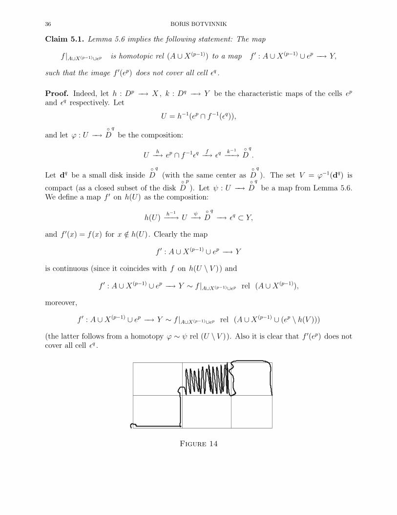
Claim 5.1. Lemma 5.6 implies the following statement: The map
f |A∪X(p−1)∪ep is homotopic rel (A ∪X(p−1)) to a map f ′ : A ∪X(p−1) ∪ ep −→ Y,
such that the image f ′(ep) does not cover all cell ǫq .
Proof. Indeed, let h : Dp −→ X , k : Dq −→ Y be the characteristic maps of the cells ep
and ǫq respectively. Let
U = h−1(ep ∩ f−1(ǫq)),
and let ϕ : U −→Dq
be the composition:
Uh−→ ep ∩ f−1ǫq
f−→ ǫqk−1
−−→Dq
.
Let dq be a small disk insideDq
(with the same center asDq
). The set V = ϕ−1(dq) is
compact (as a closed subset of the diskDp
). Let ψ : U −→Dq
be a map from Lemma 5.6.We define a map f ′ on h(U) as the composition:
h(U)h−1
−−→ Uψ−→
Dq
−→ ǫq ⊂ Y,
and f ′(x) = f(x) for x /∈ h(U). Clearly the map
f ′ : A ∪X(p−1) ∪ ep −→ Y
is continuous (since it coincides with f on h(U \ V )) and
f ′ : A ∪X(p−1) ∪ ep −→ Y ∼ f |A∪X(p−1)∪ep rel (A ∪X(p−1)),
moreover,
f ′ : A ∪X(p−1) ∪ ep −→ Y ∼ f |A∪X(p−1)∪ep rel (A ∪X(p−1) ∪ (ep \ h(V )))
(the latter follows from a homotopy ϕ ∼ ψ rel (U \ V )). Also it is clear that f ′(ep) does notcover all cell ǫq .
Figure 14
NOTES ON THE COURSE “ALGEBRAIC TOPOLOGY” 37
Figure 15
5.3. Completion of the proof of Theorem 5.5. Now the argument is simple. Firstly, ahomotopy between the maps
f |A∪X(p−1)∪ep and f ′ rel (A ∪X(p−1))
can be extend to all X by Borsuk Theorem. In particular, we can assume that f ′ with allabove properties is defined on all X .
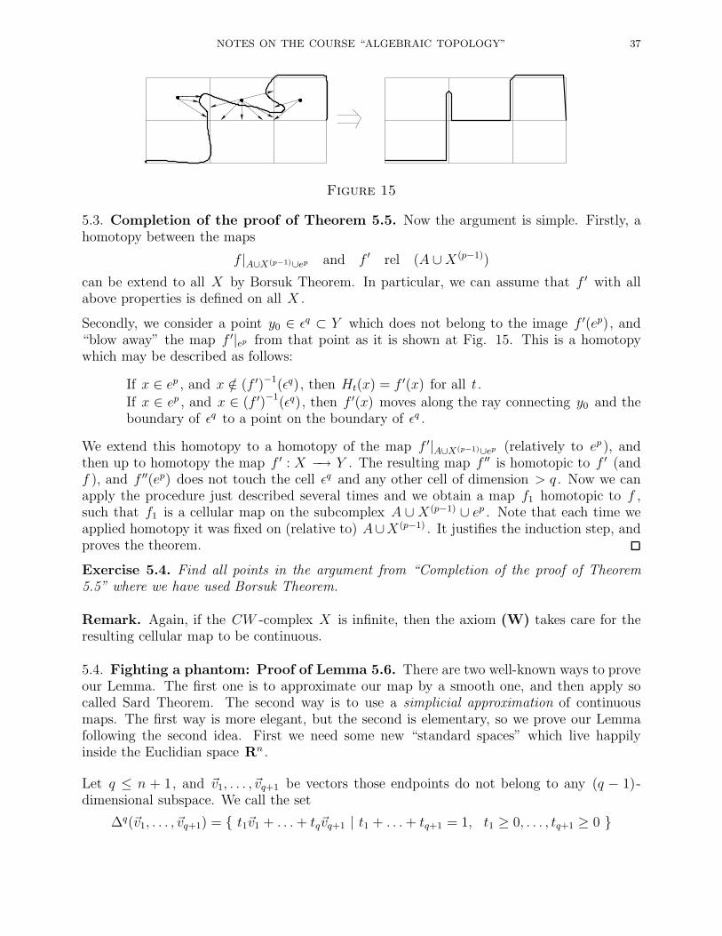
Secondly, we consider a point y0 ∈ ǫq ⊂ Y which does not belong to the image f ′(ep), and“blow away” the map f ′|ep from that point as it is shown at Fig. 15. This is a homotopywhich may be described as follows:
If x ∈ ep , and x /∈ (f ′)−1(ǫq), then Ht(x) = f ′(x) for all t.
If x ∈ ep , and x ∈ (f ′)−1(ǫq), then f ′(x) moves along the ray connecting y0 and theboundary of ǫq to a point on the boundary of ǫq .
We extend this homotopy to a homotopy of the map f ′|A∪X(p−1)∪ep (relatively to ep ), andthen up to homotopy the map f ′ : X −→ Y . The resulting map f ′′ is homotopic to f ′ (andf ), and f ′′(ep) does not touch the cell ǫq and any other cell of dimension > q . Now we canapply the procedure just described several times and we obtain a map f1 homotopic to f ,such that f1 is a cellular map on the subcomplex A ∪ X(p−1) ∪ ep . Note that each time weapplied homotopy it was fixed on (relative to) A∪X(p−1) . It justifies the induction step, andproves the theorem.
Exercise 5.4. Find all points in the argument from “Completion of the proof of Theorem5.5” where we have used Borsuk Theorem.
Remark. Again, if the CW -complex X is infinite, then the axiom (W) takes care for theresulting cellular map to be continuous.
5.4. Fighting a phantom: Proof of Lemma 5.6. There are two well-known ways to proveour Lemma. The first one is to approximate our map by a smooth one, and then apply socalled Sard Theorem. The second way is to use a simplicial approximation of continuousmaps. The first way is more elegant, but the second is elementary, so we prove our Lemmafollowing the second idea. First we need some new “standard spaces” which live happilyinside the Euclidian space Rn .
Let q ≤ n + 1, and ~v1, . . . , ~vq+1 be vectors those endpoints do not belong to any (q − 1)-dimensional subspace. We call the set
∆q(~v1, . . . , ~vq+1) = t1~v1 + . . .+ tq~vq+1 | t1 + . . .+ tq+1 = 1, t1 ≥ 0, . . . , tq+1 ≥ 0
38 BORIS BOTVINNIK
a q -dimensional simplex.
Exercise 5.5. ∆(~v1, . . . , ~vq+1) is homeomorphic (moreover, by means of a linear map) to thestandard simplex
∆q =(x1, . . . , xq+1) ∈ Rq+1 | x1 ≥ 0, . . . , xq+1 ≥ 0,
∑q+1i=1 xi = 1
.
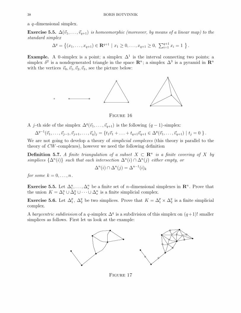
Example. A 0-simplex is a point; a simplex ∆1 is the interval connecting two points; asimplex δ2 is a nondegenerated triangle in the space Rn ; a simplex ∆3 is a pyramid in Rn
with the vertices ~v0, ~v1, ~v2, ~v3 , see the picture below:
Figure 16
A j -th side of the simplex ∆q(~v1, . . . , ~vq+1) is the following (q − 1)-simplex:
∆q−1(~v1, . . . , ~vj−1, ~vj+1, . . . , ~vq)j = t1~v1 + . . .+ tq+1~vq+1 ∈ ∆q(~v1, . . . , ~vq+1) | tj = 0 .We are not going to develop a theory of simplicial complexes (this theory is parallel to thetheory of CW -complexes), however we need the following definition
Definition 5.7. A finite triangulation of a subset X ⊂ Rn is a finite covering of X bysimplices ∆n(i) such that each intersection ∆n(i) ∩∆n(j) either empty, or
∆n(i) ∩∆n(j) = ∆n−1(i)k
for some k = 0, . . . , n.
Exercise 5.5. Let ∆n1 , . . . ,∆
ns be a finite set of n-dimensional simplexes in Rn . Prove that
the union K = ∆n1 ∪∆n
2 ∪ · · · ∪∆ns is a finite simplicial complex.
Exercise 5.6. Let ∆p1 , ∆q
2 be two simplices. Prove that K = ∆p1 ×∆q
2 is a finite simplicialcomplex.
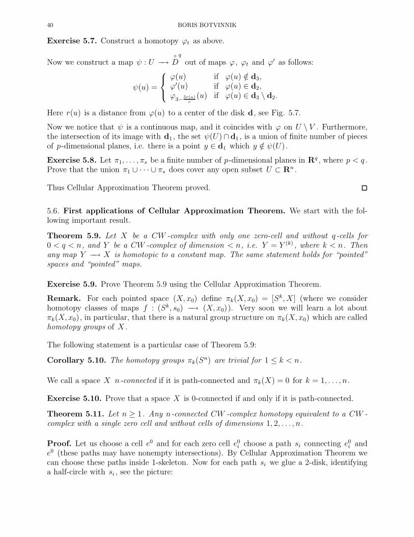
A barycentric subdivision of a q -simplex ∆q is a subdivision of this simplex on (q+1)! smallersimplices as follows. First let us look at the example:
Figure 17

NOTES ON THE COURSE “ALGEBRAIC TOPOLOGY” 39
In general, we can proceed by induction. The picture above shows a barycentric subdivisionof the simplices ∆1 , and ∆2 . Assume by induction that we have defined a barycentricsubdivision of the simplices ∆j for j ≤ q − 1. Now let x∗ be a weight center of the simplex∆q . We already have a barycentric subdivision of each j -the side ∆q
j by (q − 1)-simplices
∆(1)j , . . . ,∆
(n)j , n = q!. The cones over these simplices, j = 0, . . . , q , with a vertex x∗
constitute a barycentric subdivision of ∆q . Now we will prove the following “ApproximationLemma”:
Lemma 5.8. Let V ⊂ U be two open sets of Rn such that their closure V , U are compactsets and V ⊂ U . Then there exists a finite triangulation of V by n-simplices ∆n(i) suchthat ∆n(i) ⊂ U .
Proof. For each point x ∈ V there exists a simplex ∆n(x) with a center at x and ∆n(x) ⊂ U .By compactness of V there exist a finite number of simplices ∆n(xi) covering V . It remains touse Exercise 5.6 to conclude that a union of finite number of ∆n(xi) has a finite triangulation.
5.5. Back to the Proof of Lemma 5.6. We consider carefully our map ϕ : U −→Dq
.First we construct the disks d1 , d2 , d3 , d4 inside the disk d with the same center and of radiir/5, 2r/5, 3r/5, 4r/5 respectively, where r is a radius of d . Then we cover V = ϕ−1(d) byfinite number of p-simplexes ∆p(j), such that ∆n(j) ⊂ U . Making, if necessary, a barycentricsubdivision (a finite number of times) of these simplices, we can assume that each simplex∆p has a diameter d(ϕ(∆p)) < r/5. Let K1 be a union of all simplices ∆q such that theintersection ϕ(∆) ∩ d4 is not empty. Then
d4 ∩ ϕ(U) ⊂ ϕ(K1) ⊂ d.
Now we consider a map ϕ′ : K1 −→ d4 which coincides with ϕ on all vertices of our trian-gulation, and is linear on each simplex ∆ ⊂ K1 . The maps ϕ|K1 and ϕ′ are homotopic, i.e.there is a homotopy ϕt : K1 −→ d4 , such that ϕ0 = ϕ|K1 and ϕ1 = ϕ′ .
ϕ=ψ ϕ
ψ
ϕ′ϕ′=ψ
ϕ=ψ
Figure 18
40 BORIS BOTVINNIK
Exercise 5.7. Construct a homotopy ϕt as above.
Now we construct a map ψ : U −→Dq
out of maps ϕ , ϕt and ϕ′ as follows:
ψ(u) =
ϕ(u) if ϕ(u) /∈ d3,ϕ′(u) if ϕ(u) ∈ d2,ϕ
3− 5r(u)r
(u) if ϕ(u) ∈ d3 \ d2.
Here r(u) is a distance from ϕ(u) to a center of the disk d, see Fig. 5.7.
Now we notice that ψ is a continuous map, and it coincides with ϕ on U \ V . Furthermore,the intersection of its image with d1 , the set ψ(U) ∩d1 , is a union of finite number of piecesof p-dimensional planes, i.e. there is a point y ∈ d1 which y /∈ ψ(U).
Exercise 5.8. Let π1, . . . , πs be a finite number of p-dimensional planes in Rq , where p < q .Prove that the union π1 ∪ · · · ∪ πs does cover any open subset U ⊂ Rn .
Thus Cellular Approximation Theorem proved.
5.6. First applications of Cellular Approximation Theorem. We start with the fol-lowing important result.
Theorem 5.9. Let X be a CW -complex with only one zero-cell and without q -cells for0 < q < n, and Y be a CW -complex of dimension < n, i.e. Y = Y (k) , where k < n. Thenany map Y −→ X is homotopic to a constant map. The same statement holds for “pointed”spaces and “pointed” maps.
Exercise 5.9. Prove Theorem 5.9 using the Cellular Approximation Theorem.
Remark. For each pointed space (X, x0) define πk(X, x0) = [Sk, X] (where we considerhomotopy classes of maps f : (Sk, s0) −→ (X, x0)). Very soon we will learn a lot aboutπk(X, x0), in particular, that there is a natural group structure on πk(X, x0) which are calledhomotopy groups of X .
The following statement is a particular case of Theorem 5.9:
Corollary 5.10. The homotopy groups πk(Sn) are trivial for 1 ≤ k < n.
We call a space X n-connected if it is path-connected and πk(X) = 0 for k = 1, . . . , n.
Exercise 5.10. Prove that a space X is 0-connected if and only if it is path-connected.
Theorem 5.11. Let n ≥ 1. Any n-connected CW -complex homotopy equivalent to a CW -complex with a single zero cell and without cells of dimensions 1, 2, . . . , n.
Proof. Let us choose a cell e0 and for each zero cell e0i choose a path si connecting e0i ande0 (these paths may have nonempty intersections). By Cellular Approximation Theorem wecan choose these paths inside 1-skeleton. Now for each path si we glue a 2-disk, identifyinga half-circle with si , see the picture:
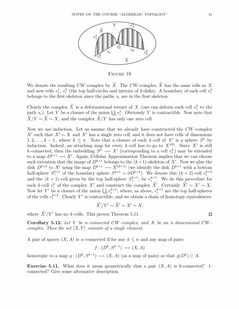
NOTES ON THE COURSE “ALGEBRAIC TOPOLOGY” 41
Xe01
s1
e00 s2 e02
X
Y
e11
e12
Figure 19
We denote the resulting CW -complex by X . The CW -complex X has the same cells as Xand new cells e1i , e
2i (the top half-circles and interior of 2-disks). A boundary of each cell e2i
belongs to the first skeleton since the paths si are in the first skeleton.
Clearly the complex X is a deformational retract of X (one can deform each cell e2i to thepath si ). Let Y be a closure of the union
⋃i e
1i . Obviously Y is contractible. Now note that
X/Y ∼ X ∼ X , and the complex X/Y has only one zero cell.
Now we use induction. Let us assume that we already have constructed the CW -complexX ′ such that X ′ ∼ X and X ′ has a single zero cell, and it does not have cells of dimensions1, 2, . . . , k − 1, where k ≤ n. Note that a closure of each k -cell of X ′ is a sphere Sk byinduction. Indeed, an attaching map for every k -cell has to go to X ′(0) . Since X ′ is stillk -connected, then the embedding Sk −→ X ′ (corresponding to a cell eki ) may be extendedto a map Dk+1 −→ X ′ . Again, Cellular Approximation Theorem implies that we can choosesuch extention that the image of Dk+1 belongs to the (k+1)-skeleton of X ′ . Now we glue thedisk Dk+2 to X ′ using the map Dk+1 −→ X ′(k+1) (we identify the disk Dk+1 with a bottomhalf-sphere Sk+1
− of the boundary sphere Sk+1 = ∂Dk+2 ). We denote this (k + 2)-cell ek+2i
and the (k + 1)-cell given by the top half-sphere Sk+1+ , by ek+1
i . We do this procedure for
each k -cell eki of the complex X ′ and construct the complex X ′ . Certainly X ′ ∼ X ′ ∼ X .Now let Y ′ be a closure of the union
⋃i ek+1i , where, as above, ek+1
i are the top half-spheres
of the cells ek+2i . Clearly Y ′ is contractible, and we obtain a chain of homotopy equivalences:
X ′/Y ′ ∼ X ′ ∼ X ′ ∼ X,
where X ′/Y ′ has no k -cells. This proves Theorem 5.11.
Corollary 5.12. Let Y be n-connected CW -complex, and X be an n-dimensional CW -complex. Then the set [X, Y ] consists of a single element.
A pair of spaces (X,A) is n-connected if for any k ≤ n and any map of pairs
f : (Dk, Sk−1) −→ (X,A)
homotopic to a map g : (Dk, Sk−1) −→ (X,A) (as a map of pairs) so that g(Dk) ⊂ A.
Exercise 5.11. What does it mean geometrically that a pair (X,A) is 0-connected? 1-connected? Give some alternative description.

42 BORIS BOTVINNIK
Exercise 5.12. Let (X,A) be an n-connected pair of CW -complexes. Prove that (X,A) ishomotopy equivalent to a CW -pair (Y,B) so that B ⊂ Y (n) .
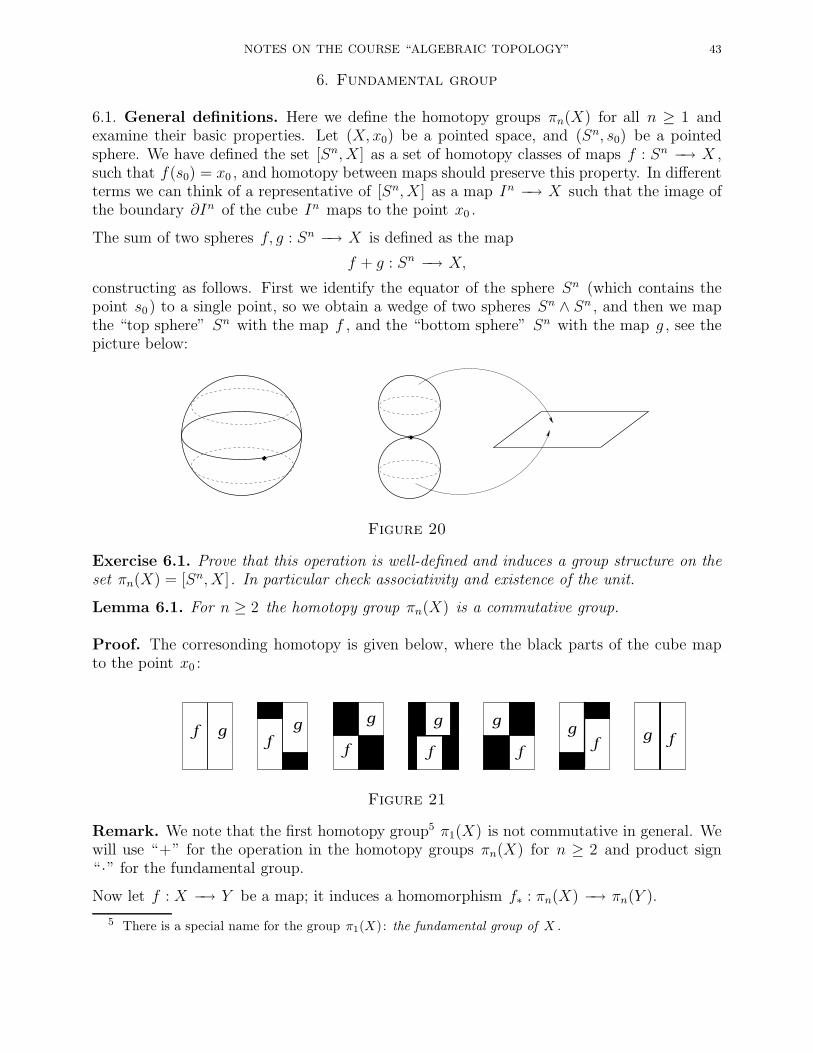
NOTES ON THE COURSE “ALGEBRAIC TOPOLOGY” 43
6. Fundamental group
6.1. General definitions. Here we define the homotopy groups πn(X) for all n ≥ 1 andexamine their basic properties. Let (X, x0) be a pointed space, and (Sn, s0) be a pointedsphere. We have defined the set [Sn, X] as a set of homotopy classes of maps f : Sn −→ X ,such that f(s0) = x0 , and homotopy between maps should preserve this property. In differentterms we can think of a representative of [Sn, X] as a map In −→ X such that the image ofthe boundary ∂In of the cube In maps to the point x0 .
The sum of two spheres f, g : Sn −→ X is defined as the map
f + g : Sn −→ X,
constructing as follows. First we identify the equator of the sphere Sn (which contains thepoint s0 ) to a single point, so we obtain a wedge of two spheres Sn ∧ Sn , and then we mapthe “top sphere” Sn with the map f , and the “bottom sphere” Sn with the map g , see thepicture below:
Figure 20
Exercise 6.1. Prove that this operation is well-defined and induces a group structure on theset πn(X) = [Sn, X]. In particular check associativity and existence of the unit.
Lemma 6.1. For n ≥ 2 the homotopy group πn(X) is a commutative group.
Proof. The corresonding homotopy is given below, where the black parts of the cube mapto the point x0 :
gf
g
f
g
f
g g
f
gf
g ff
Figure 21
Remark. We note that the first homotopy group5 π1(X) is not commutative in general. Wewill use “+” for the operation in the homotopy groups πn(X) for n ≥ 2 and product sign“·” for the fundamental group.
Now let f : X −→ Y be a map; it induces a homomorphism f∗ : πn(X) −→ πn(Y ).
5 There is a special name for the group π1(X): the fundamental group of X .
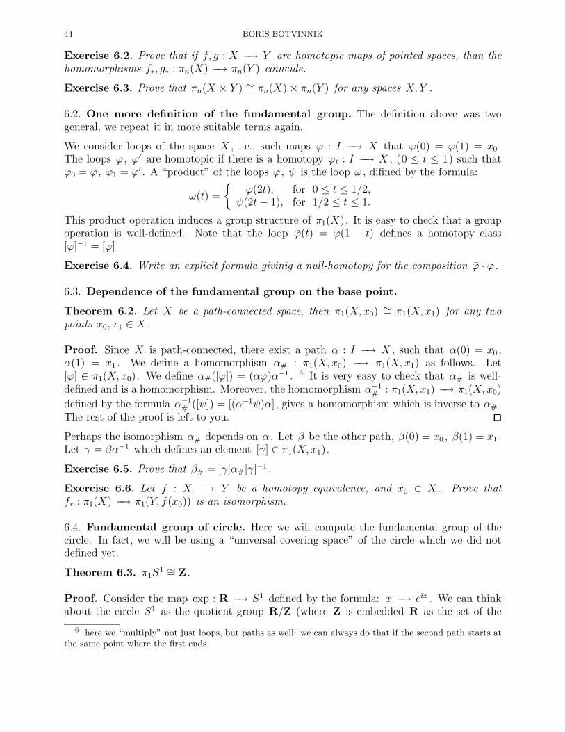
44 BORIS BOTVINNIK
Exercise 6.2. Prove that if f, g : X −→ Y are homotopic maps of pointed spaces, than thehomomorphisms f∗, g∗ : πn(X) −→ πn(Y ) coincide.
Exercise 6.3. Prove that πn(X × Y ) ∼= πn(X)× πn(Y ) for any spaces X, Y .
6.2. One more definition of the fundamental group. The definition above was twogeneral, we repeat it in more suitable terms again.
We consider loops of the space X , i.e. such maps ϕ : I −→ X that ϕ(0) = ϕ(1) = x0 .The loops ϕ , ϕ′ are homotopic if there is a homotopy ϕt : I −→ X , (0 ≤ t ≤ 1) such thatϕ0 = ϕ , ϕ1 = ϕ′ . A “product” of the loops ϕ , ψ is the loop ω , difined by the formula:
ω(t) =
ϕ(2t), for 0 ≤ t ≤ 1/2,
ψ(2t− 1), for 1/2 ≤ t ≤ 1.
This product operation induces a group structure of π1(X). It is easy to check that a groupoperation is well-defined. Note that the loop ϕ(t) = ϕ(1 − t) defines a homotopy class[ϕ]−1 = [ϕ]
Exercise 6.4. Write an explicit formula givinig a null-homotopy for the composition ϕ · ϕ.
6.3. Dependence of the fundamental group on the base point.
Theorem 6.2. Let X be a path-connected space, then π1(X, x0) ∼= π1(X, x1) for any twopoints x0, x1 ∈ X .
Proof. Since X is path-connected, there exist a path α : I −→ X , such that α(0) = x0 ,α(1) = x1 . We define a homomorphism α# : π1(X, x0) −→ π1(X, x1) as follows. Let[ϕ] ∈ π1(X, x0). We define α#([ϕ]) = (αϕ)α−1 . 6 It is very easy to check that α# is well-defined and is a homomorphism. Moreover, the homomorphism α−1
# : π1(X, x1) −→ π1(X, x0)
defined by the formula α−1# ([ψ]) = [(α−1ψ)α], gives a homomorphism which is inverse to α# .
The rest of the proof is left to you.
Perhaps the isomorphism α# depends on α . Let β be the other path, β(0) = x0 , β(1) = x1 .Let γ = βα−1 which defines an element [γ] ∈ π1(X, x1).
Exercise 6.5. Prove that β# = [γ]α#[γ]−1 .
Exercise 6.6. Let f : X −→ Y be a homotopy equivalence, and x0 ∈ X . Prove thatf∗ : π1(X) −→ π1(Y, f(x0)) is an isomorphism.
6.4. Fundamental group of circle. Here we will compute the fundamental group of thecircle. In fact, we will be using a “universal covering space” of the circle which we did notdefined yet.
Theorem 6.3. π1S1 ∼= Z.
Proof. Consider the map exp : R −→ S1 defined by the formula: x −→ eix . We can thinkabout the circle S1 as the quotient group R/Z (where Z is embedded R as the set of the
6 here we “multiply” not just loops, but paths as well: we can always do that if the second path starts atthe same point where the first ends

NOTES ON THE COURSE “ALGEBRAIC TOPOLOGY” 45
numbers 2πk , k = 0,±1,±2, . . .). A loop ϕ : I −→ S1 (ϕ(0) = ϕ(1) = e0 ) may be lifted toa map ϕ : I −→ R . It means that ϕ is decomposed as
ϕ : Ieϕ−→ R
exp−−→ R/Z = S1,
where ϕ(0) = 0 and ϕ(1) = 2πk for some integer k . Note that a lifting ϕ : I −→ R with theabove properties is unique.
Note that if the loops ϕ, ϕ′ : I −→ S1 are homotopic, then the paths ϕ , ϕ′ have the sameend point 2πk (since we cannot “jump” from 2πk to 2πl if l 6= k by means of continuoushomotopy!). Now the isomorphism π1
∼= Z becomes almost obvious: [ϕ] −→ k ∈ Z. Itremains to see that the loop ϕ : I −→ S1 (ϕ : I −→ R , where ϕ(0) = 0 and ϕ(1) = 2πk ) is
homotopic to the “standatrd loop” hk going from 0 to 2πk , see picture below:
Figure 22
It remains to observe that hkhl ∼ hk+l .
Theorem 6.4. Let XA =∨
α∈AS1α . Then π1(XA) is a free group with generators ηα , α ∈ A.
Proof. Let iα : S1 −→ XA be an embedding of the corresponding circle. Let ηα ∈ π1(XA)be the element given by iα . We prove the following statement.
Claim 6.1. 1o Any element β ∈ π1(XA) may be represented as a finite product of elementsηα , η−1
α , α ∈ A:
(13) β = ηǫ1α1· · · ηǫsαs
, ǫj = ±1.
2o The presentation (13) is unique up to cancelation of the elements ηαη−1α or η−1
α ηα .
Claim 6.1 is equivalent to Theorem 6.4. Now we prove 1o , and we postpone 2o to the nextsection.
Proof of 1o . Let Iα , Jα be two closed intervals in the circle, Jα ⊂ IntIα , and Iα does notcontain the base point.
Jα ⊂ Iα Jα′ ⊂ Iα′
Now let ϕ : I −→ XA be a loop. We find n such that for anyinterval J of the length 1/n if the intersection ϕ(J)∩ Jα 6= ∅ ,then ϕ(J) ⊂ Iα . Let K be the following union:
K =⋃
ϕ([k/n,(k+1)/n])∩(∪αJα)6=∅[k/n, (k + 1)/n].
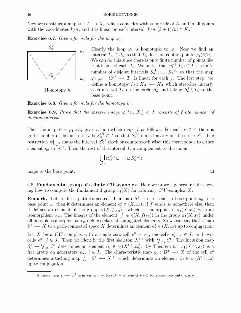
46 BORIS BOTVINNIK
Now we construct a map ϕ1 : I −→ XA which coincides with ϕ outside of K and in all pointswith the coordinates k/n, and it is linear on each interval [k/n, (k + 1)/n] ⊂ K .7
Exercise 6.7. Give a formula for the map ϕ1 .
Tα
S1α
h0
h1
Homotopy ht
Clearly the loop ϕ1 is homotopic to ϕ . Now we find aninterval Tα ⊂ Jα , so that Tα does not contain points ϕ1(k/n).We can do this since there is only finite number of points likethat inside of each Jα . We notice that ϕ−1
1 (Tα) ⊂ I is a finite
number of disjoint intervals S(1)α , . . . , S
(rα)α so that the map
ϕ1|S(j)α
: S(j)α −→ Tα is linear for each j . The last step: we
define a homotopy ht : XA −→ XA which stretches linearlyeach interval Tα on the circle S1
α and taking S1α \ Tα to the
base point.
Exercise 6.8. Give a formula for the homotopy ht .
Exercise 6.9. Prove that the inverse image ϕ−11 (∪αTα) ⊂ I consists of finite number of
disjoint intervals.
Then the map ψ = ϕ1 h1 gives a loop which maps I as follows. For each α ∈ A there is
finite number of disjoint intervals S(j)α ⊂ I so that S
(j)α maps linearly on the circle S1
α . The
restriction ψ|S
(j)α
maps the interval S(j)α clock or counterclock wise; this corresponds to either
element ηα or η−1α . Then the rest of the interval I , a complement to the union
⋃
α∈A(S(1)
α ⊔ · · · ⊔ S(rα)α )
maps to the base point.
6.5. Fundamental group of a finite CW -complex. Here we prove a general result show-ing how to compute the fundamental group π1(X) for arbitrary CW -complex X .
Remark. Let X be a path-connected. If a map S1 −→ X sends a base point s0 to abase point x0 then it determines an element of π1(X, x0); if f sends s0 somethere else, thenit defines an element of the group π(X, f(s0)), which is isomorphic to π1(X, x0) with anisomorphism α# . The images of the element [f ] ∈ π(X, f(s0)) in the group π1(X, x0) underall possible isomorphisms α# define a class of conjugated elements. So we can say that a mapS1 −→ X to a path-connected space X determines an element of π1(X, x0) up to conjugation.
Let X be a CW -complex with a single zero-cell e0 = x0 , one-cells e1i , i ∈ I , and two-cells e2j , j ∈ J . Then we identify the first skeleton X(1) with
∨i∈I S
1i . The inclusion map
S1i →
∨i∈I S
1i determines an element αi ∈ π1(X
(1), x0). By Theorem 6.4 π1(X(1), x0) is a
free group on generators αi , i ∈ I . The characteristic map gj : D2 −→ X of the cell e2jdetermines attaching map fj : S1 −→ X(1) which determines an element βj ∈ π1(X
(1), x0)up to conjugation.
7 A linear map I −→ S1 is given by t 7→ (cos(λt+ µ), sin(λt+ ν)) for some constants λ, µ, ν .

NOTES ON THE COURSE “ALGEBRAIC TOPOLOGY” 47
Theorem 6.5. Let X be a CW -complex with a single zero cell e0 , one-cells e1i (i ∈ I ),and two-cells e2j (j ∈ J ). Let αi be the generators of π1(X
(1), x0) corresponding to the the
cells e1i , and βj ∈ π1(X(1), x0) = F (αi | i ∈ I) be elements determined by the attaching maps
fj : S1 −→ X1 of the cells e2j . Then
1. π1(X, x0) ∼= π1(X(2), x0);
2. π1(X, x0) is a group on generators αi , i ∈ I , and relations βj = 1, j ∈ J .
Proof. We consider the circle S1 as 1-dimensional CW -complex. Cellular ApproximationTheorem implies then that any loop S1 −→ X homotopic to a loop in the first skeleton, i.e.the homomorphism
ι∗ : π1(X(1), x0) −→ π1(X, x0)
induced by the inclusion ι : X(1) −→ X , is an epimorphism. It is enough to prove thatKer i∗ is generated by βj , j ∈ J . It is clear that βj ∈ Ker ι∗ . Indeed, the attaching mapfj : S1 −→ X(1) is extended to the characteristic map gj : D2 −→ X , and determines atrivial element in the group π1(X, fj(s0)); and this element corresponds to βj under someisomorphism π1(X, fj(s0)) ∼= π1(X, x0).
It is more difficult to prove that if γ ∈ Ker i∗ then γ may be presented as a product ofelements β±
j : here we will apply again the Cellular Approximation Theorem. We identify
each cell e2j with the open disk D2j in R2 , so we can construct disks d(j) ⊂ D2
j of radius r(j) ,
and disks d(j)1 , d
(j)2 , d
(j)3 and d
(j)4 (with the same center) of radius r(j)/5, 2r(j)/5, 3r(j)/5 and
4r(j)/5 respectively.
Now let ϕ : S1 −→ X(1) be a representative of an element γ ∈ Ker i∗ . Clearly there is anextension Φ : D2 −→ X of the map ϕ . By the Cellular Approximation Theorem we canassume that Φ(D2) ⊂ X(2) . We triangulate D2 in such way that if ∆ is a triangle from this
triangulation such that Φ(∆) ∩ d(j)4 6= ∅ , then
(a) Φ(∆) ⊂ d(j) and
(b) diam(Φ(∆) < r(j)/5.
Let K be a union of all triangles ∆ of our triangulation such that
Φ(∆) ∩(⋃
j∈Jd
(j)4
)6= ∅.
Now we make the map Φ′ : K −→ X(2) which concides with Φ on the vertexes of each simplexand is linear on each simplex ∆. The maps Φ′ and Φ|K are homotopic (inside the cell e2j ) bymeans of a homotopy Φt = (1− t)Φ + tΦ′ , with Φ0 = Φ|K , Φ1 = Φ′ . Now we use a familiarformula
Φ′′(u) =
Φ(u), if Φ(u) /∈ ⋃j d(j)3
Φ′(u), if Φ(u) ∈ ⋃j d(j)2
Φ3− 5r(u)
rj
(u), if Φ(u) ∈ d(j)3 \ d(j)
2
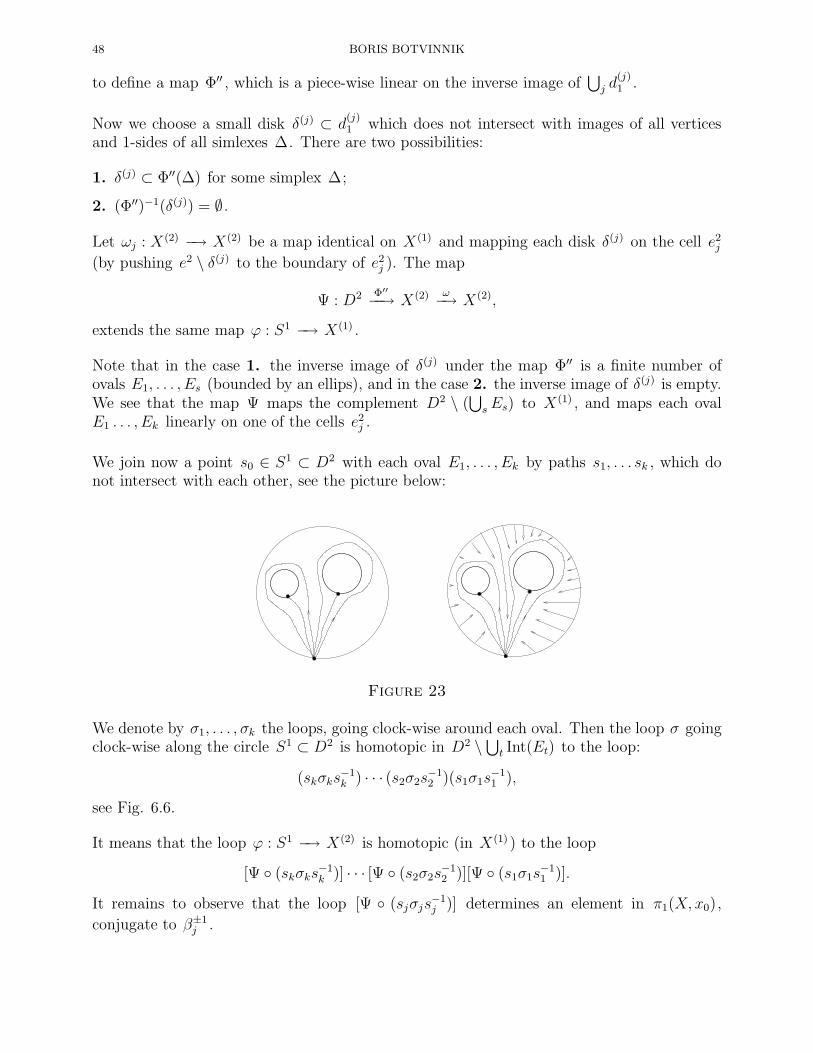
48 BORIS BOTVINNIK
to define a map Φ′′ , which is a piece-wise linear on the inverse image of⋃j d
(j)1 .
Now we choose a small disk δ(j) ⊂ d(j)1 which does not intersect with images of all vertices
and 1-sides of all simlexes ∆. There are two possibilities:
1. δ(j) ⊂ Φ′′(∆) for some simplex ∆;
2. (Φ′′)−1(δ(j)) = ∅ .
Let ωj : X(2) −→ X(2) be a map identical on X(1) and mapping each disk δ(j) on the cell e2j(by pushing e2 \ δ(j) to the boundary of e2j ). The map
Ψ : D2 Φ′′
−−→ X(2) ω−→ X(2),
extends the same map ϕ : S1 −→ X(1) .
Note that in the case 1. the inverse image of δ(j) under the map Φ′′ is a finite number ofovals E1, . . . , Es (bounded by an ellips), and in the case 2. the inverse image of δ(j) is empty.We see that the map Ψ maps the complement D2 \ (
⋃sEs) to X(1) , and maps each oval
E1 . . . , Ek linearly on one of the cells e2j .
We join now a point s0 ∈ S1 ⊂ D2 with each oval E1, . . . , Ek by paths s1, . . . sk , which donot intersect with each other, see the picture below:
Figure 23
We denote by σ1, . . . , σk the loops, going clock-wise around each oval. Then the loop σ goingclock-wise along the circle S1 ⊂ D2 is homotopic in D2 \⋃t Int(Et) to the loop:
(skσks−1k ) · · · (s2σ2s
−12 )(s1σ1s
−11 ),
see Fig. 6.6.
It means that the loop ϕ : S1 −→ X(2) is homotopic (in X(1) ) to the loop
[Ψ (skσks−1k )] · · · [Ψ (s2σ2s
−12 )][Ψ (s1σ1s
−11 )].
It remains to observe that the loop [Ψ (sjσjs−1j )] determines an element in π1(X, x0),
conjugate to β±1j .
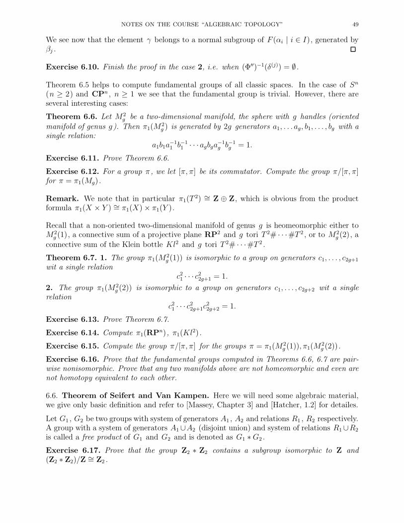
NOTES ON THE COURSE “ALGEBRAIC TOPOLOGY” 49
We see now that the element γ belongs to a normal subgroup of F (αi | i ∈ I), generated byβj .
Exercise 6.10. Finish the proof in the case 2, i.e. when (Φ′′)−1(δ(j)) = ∅.
Theorem 6.5 helps to compute fundamental groups of all classic spaces. In the case of Sn
(n ≥ 2) and CPn , n ≥ 1 we see that the fundamental group is trivial. However, there areseveral interesting cases:
Theorem 6.6. Let M2g be a two-dimensional manifold, the sphere with g handles (oriented
manifold of genus g ). Then π1(M2g ) is generated by 2g generators a1, . . . ag, b1, . . . , bg with a
single relation:a1b1a
−11 b−1
1 · · ·agbga−1g b−1
g = 1.
Exercise 6.11. Prove Theorem 6.6.
Exercise 6.12. For a group π , we let [π, π] be its commutator. Compute the group π/[π, π]for π = π1(Mg).
Remark. We note that in particular π1(T2) ∼= Z ⊕ Z, which is obvious from the product
formula π1(X × Y ) ∼= π1(X)× π1(Y ).
Recall that a non-oriented two-dimensional manifold of genus g is heomeomorphic either toM2
g (1), a connective sum of a projective plane RP2 and g tori T 2# · · ·#T 2 , or to M2g (2), a
connective sum of the Klein bottle Kl2 and g tori T 2# · · ·#T 2 .
Theorem 6.7. 1. The group π1(M2g (1)) is isomorphic to a group on generators c1, . . . , c2g+1
wit a single relationc21 · · · c22g+1 = 1.
2. The group π1(M2g (2)) is isomorphic to a group on generators c1, . . . , c2g+2 wit a single
relationc21 · · · c22g+1c
22g+2 = 1.
Exercise 6.13. Prove Theorem 6.7.
Exercise 6.14. Compute π1(RPn), π1(Kl2).
Exercise 6.15. Compute the group π/[π, π] for the groups π = π1(M2g (1)), π1(M
2g (2)).
Exercise 6.16. Prove that the fundamental groups computed in Theorems 6.6, 6.7 are pair-wise nonisomorphic. Prove that any two manifolds above are not homeomorphic and even arenot homotopy equivalent to each other.
6.6. Theorem of Seifert and Van Kampen. Here we will need some algebraic material,we give only basic definition and refer to [Massey, Chapter 3] and [Hatcher, 1.2] for detailes.
Let G1 , G2 be two groups with system of generators A1 , A2 and relations R1 , R2 respectively.A group with a system of generators A1∪A2 (disjoint union) and system of relations R1∪R2
is called a free product of G1 and G2 and is denoted as G1 ∗G2 .
Exercise 6.17. Prove that the group Z2 ∗ Z2 contains a subgroup isomorphic to Z and(Z2 ∗ Z2)/Z ∼= Z2 .
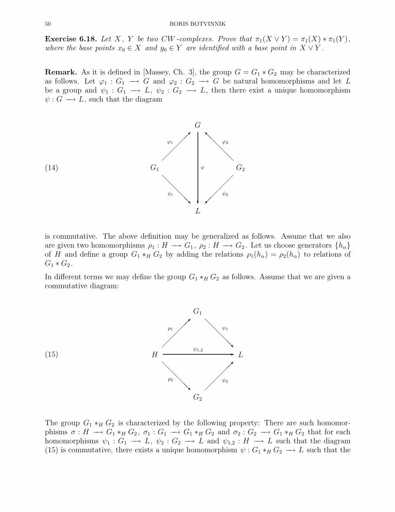
50 BORIS BOTVINNIK
Exercise 6.18. Let X , Y be two CW -complexes. Prove that π1(X ∨ Y ) = π1(X) ∗ π1(Y ),where the base points x0 ∈ X and y0 ∈ Y are identified with a base point in X ∨ Y .
Remark. As it is defined in [Massey, Ch. 3], the group G = G1 ∗ G2 may be characterizedas follows. Let ϕ1 : G1 −→ G and ϕ2 : G2 −→ G be natural homomorphisms and let Lbe a group and ψ1 : G1 −→ L, ψ2 : G2 −→ L, then there exist a unique homomorphismψ : G −→ L, such that the diagram
(14)
G
?
ψG1
ϕ1
@@
@@@R
ψi
G2
@@
@@@I ϕ2
ψ2
L
is commutative. The above definition may be generalized as follows. Assume that we alsoare given two homomorphisms ρ1 : H −→ G1 , ρ2 : H −→ G2 . Let us choose generators hαof H and define a group G1 ∗H G2 by adding the relations ρ1(hα) = ρ2(hα) to relations ofG1 ∗G2 .
In different terms we may define the group G1 ∗H G2 as follows. Assume that we are given acommutative diagram:
(15)
G1
@@
@@@R
ψ1
H
ρ1
@@
@@@R
ρ2
L-ψ1,2
G2
ψ2
The group G1 ∗H G2 is characterized by the following property: There are such homomor-phisms σ : H −→ G1 ∗H G2 , σ1 : G1 −→ G1 ∗H G2 and σ2 : G2 −→ G1 ∗H G2 that for eachhomomorphisms ψ1 : G1 −→ L, ψ2 : G2 −→ L and ψ1,2 : H −→ L such that the diagram(15) is commutative, there exists a unique homomorphism ψ : G1 ∗H G2 −→ L such that the
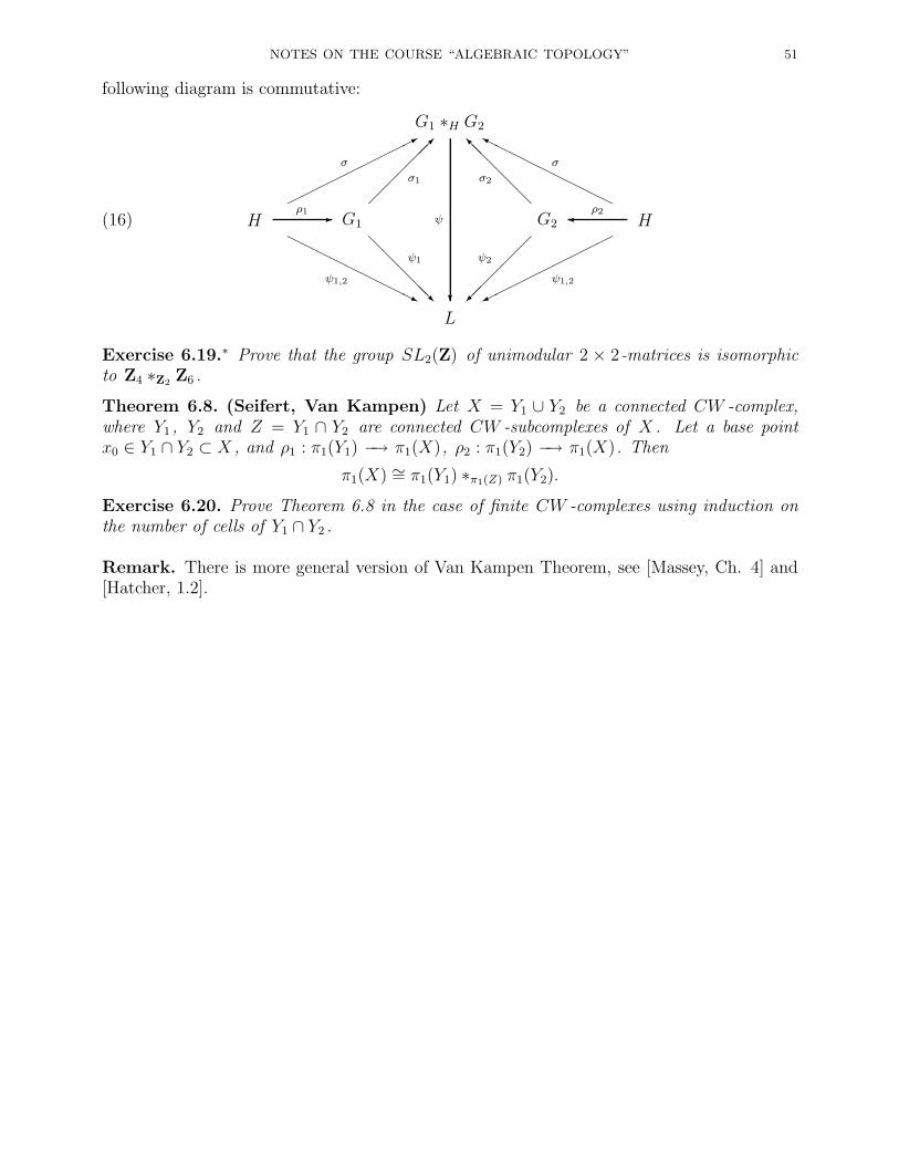
NOTES ON THE COURSE “ALGEBRAIC TOPOLOGY” 51
following diagram is commutative:
(16)
G1 ∗H G2
?
ψH
*σ
HHHHHHHHHjψ1,2
G1
@@
@@@R
ψ1
σ1
G2
ψ2
@@
@@@I
σ2
H
HHHHHHHHHYσ
ψ1,2
-ρ1 ρ2
L
Exercise 6.19.∗ Prove that the group SL2(Z) of unimodular 2 × 2-matrices is isomorphicto Z4 ∗Z2 Z6 .
Theorem 6.8. (Seifert, Van Kampen) Let X = Y1 ∪ Y2 be a connected CW -complex,where Y1 , Y2 and Z = Y1 ∩ Y2 are connected CW -subcomplexes of X . Let a base pointx0 ∈ Y1 ∩ Y2 ⊂ X , and ρ1 : π1(Y1) −→ π1(X), ρ2 : π1(Y2) −→ π1(X). Then
π1(X) ∼= π1(Y1) ∗π1(Z) π1(Y2).
Exercise 6.20. Prove Theorem 6.8 in the case of finite CW -complexes using induction onthe number of cells of Y1 ∩ Y2 .
Remark. There is more general version of Van Kampen Theorem, see [Massey, Ch. 4] and[Hatcher, 1.2].
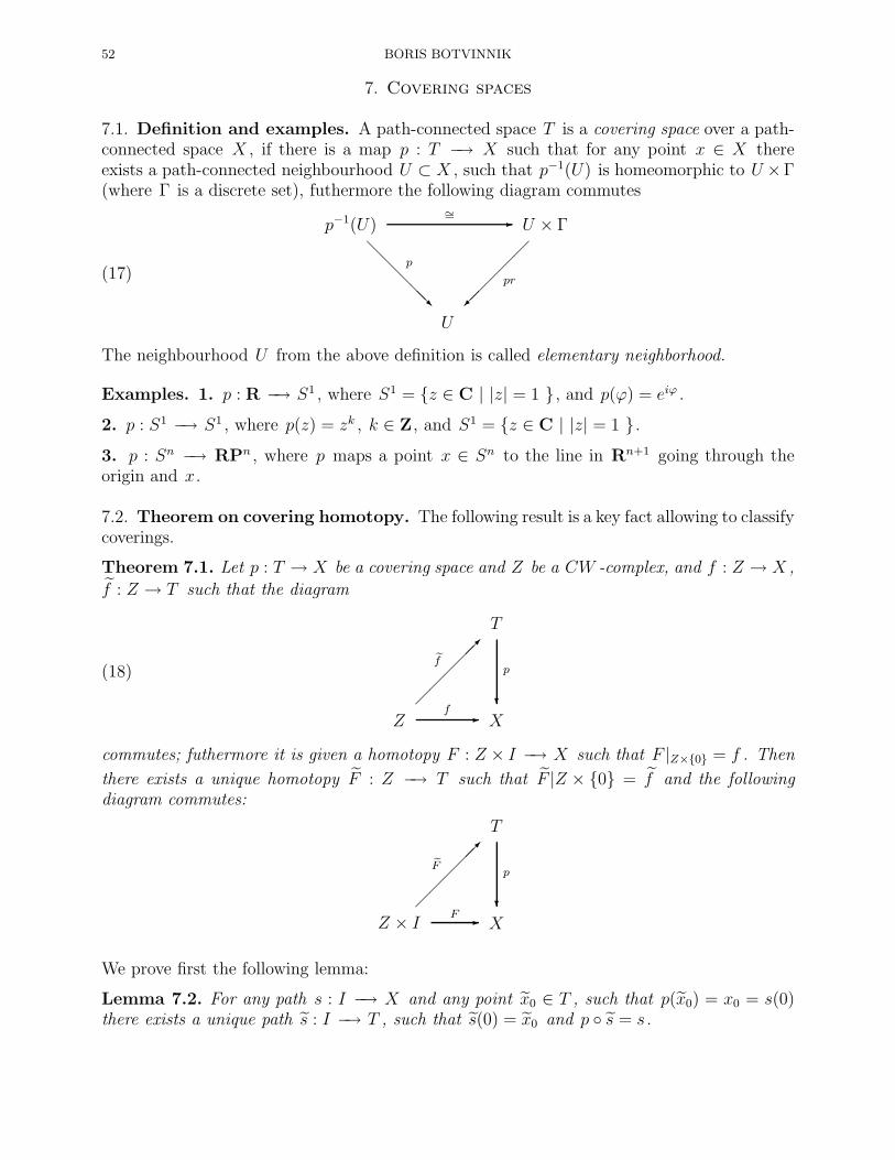
52 BORIS BOTVINNIK
7. Covering spaces
7.1. Definition and examples. A path-connected space T is a covering space over a path-connected space X , if there is a map p : T −→ X such that for any point x ∈ X thereexists a path-connected neighbourhood U ⊂ X , such that p−1(U) is homeomorphic to U ×Γ(where Γ is a discrete set), futhermore the following diagram commutes
(17)
p−1(U)
@@
@@@R
p
U × Γ
pr
-∼=
U
The neighbourhood U from the above definition is called elementary neighborhood.
Examples. 1. p : R −→ S1 , where S1 = z ∈ C | |z| = 1 , and p(ϕ) = eiϕ .
2. p : S1 −→ S1 , where p(z) = zk , k ∈ Z, and S1 = z ∈ C | |z| = 1 .3. p : Sn −→ RPn , where p maps a point x ∈ Sn to the line in Rn+1 going through theorigin and x.
7.2. Theorem on covering homotopy. The following result is a key fact allowing to classifycoverings.
Theorem 7.1. Let p : T → X be a covering space and Z be a CW -complex, and f : Z → X ,
f : Z → T such that the diagram
(18)
T
?
p
Z
ef
X-f
commutes; futhermore it is given a homotopy F : Z × I −→ X such that F |Z×0 = f . Then
there exists a unique homotopy F : Z −→ T such that F |Z × 0 = f and the followingdiagram commutes:
T
?
p
Z × I
eF
X-F
We prove first the following lemma:
Lemma 7.2. For any path s : I −→ X and any point x0 ∈ T , such that p(x0) = x0 = s(0)there exists a unique path s : I −→ T , such that s(0) = x0 and p s = s.

NOTES ON THE COURSE “ALGEBRAIC TOPOLOGY” 53
U1U2 U3 Un
U1U2 Proof. For each t ∈ I we find an elementary neighbour-
hood Ut of the point s(t). A compactness of I = [0, 1]implies that there exists a finite number of points
0 = t1 < t2 < . . . < tn = 1,such that Uj ⊃ s([tj , tj+1]). The inverse image p−1(U1) is
homeomorphic to U1 × Γ Let U1 be such that x0 ∈ U1 .Then the path s|[0,t2] : [0, t2] −→ X has a unique liftings : [0, t2] −→ T covering the path s|[0,t2] . Then we do thesame in the neighbourhood U2 and so on. Note that wehave a finite number of Uj , and in each neighbourhood Uja “lifting” is unique, see Figure to the left.
Proof of Theorem 7.1. Let z ∈ Z be any point. The formula t −→ F (z, t) defines a path
in X . Lemma 7.2 gives a unique lifting of this path to T , such that it starts at f(z). It gives
a map Z × I −→ T . This is our homotopy F .
7.3. Covering spaces and fundamental group.
Theorem 7.3. Let p : T −→ X be a covering space, then p∗ : π1(T, x0) −→ π1(X, x0) is amonomorphism (injective).
Proof: Let s : I −→ T be a loop, where s(0) = s(1) = x0 . Denote x0 = p(x0). Assume thatthe loop s = p s : I −→ X is homotopic to zero. Let st : I −→ X be such a homotopy:s0 = s, st(0) = st(1) = x0 , and s1(I) = x0 .
x0
x0
x′0
α
α
Theorem 7.1 implies that there is a homotopy st : I −→ Tcovering the homotopy st . Since the inverse image p−1(x0) is adiscrete set, then st(0) = st(1) = x0 .
The subgroup p∗(π1(T, x0)) ⊂ π1(X, x0) is called the covering
group of Tp−→ X . Let x′0 6= x0 , p(x′0) = p(x0) = x0 . Consider
a path α : I −→ T such that α(0) = x0 , α(1) = x′0 . Thenthe projection α = p(α) is a loop in X , see Figure to the left.Clearly α# : p∗(π1(T, x0)) −→ p∗(π1(T, x
′0)) given by α#(g) =
αgα−1 is an isomorphism.
Consider the coset π1(X, x0)/p∗(π1(T, x0)) (the subgroup p∗(π1(T, x0)) ⊂ π1(X, x0) is notnormal subgroup in general).
Claim 7.1. There is one-to-one correspondence p−1(x0)←→ π1(X, x0)/p∗(π1(T, x0)).
Proof. Let [γ] ∈ π1(X, x0), where γ : I −→ X ,γ(0) = γ(1) = x0 . There exists a unique liftingγ : I −→ T of γ , so that γ(0) = x0 . We defineA([γ]) = γ(1) ∈ p−1(x0), see Fig. (a). Thehomotopy lifting property implies that if γ ∼ γ′
then γ ∼ γ′ and γ(1) = γ′(1). Now let A([γ]) =A([γ′]). Then the loop β = (γ′)−1γ is covered
by the loop β = (γ′)−1γ , see Fig. (b). Thus[β] = [(γ′)−1γ] ∈ p∗(π1(T, x0)).
x0
x0
γ(1)
γ
γ
(a)
x0
x0
γ(1)
γ
γγ′
γ′
(b)

54 BORIS BOTVINNIK
This proves that A : π1(X, x0)/p∗(π1(T, x0)) −→ p−1(x0) is an injection. Clearly A is ontosince T is path-connected, and if x ∈ p−1(x0) there exists a path connecting x0 and x whichprojects to a loop in X .
Claim 7.2. Let p : T −→ X be a covering and x0, x1 ∈ X . There is one-to-one correspon-dence p−1(x0)←→ p−1(x1).
Exercise 7.1. Prove Claim 7.2. Hint: Consider a path connecting x0 and x1 .
7.4. Observation. Let γ be a loop in X , γ(0) = γ(1) = x0 , and γ : I −→ T be its liftingwith γ(0) = x0 . Then if γ(1) 6= γ(0) then the loop γ is not homotopic to zero. Indeed, ifsuch homotopy would exist, then necessarily it implies that γ(1) = γ(0).
XA
ηǫ1α1ηǫ2α2
T
We use this observation to complete the proof of The-orem 6.4, or, to be precise, the proof of Claim 6.1,2o . Indeed, let β = ηǫ1α1
· · · ηǫsαs, ǫj = ±1, where
all elements ηαη−1α , η−1
α ηα are canceled It is enoughto show that β 6= e, where e is the identity elele-ment. Recall that ηα is given by the inclusion S1
α −→∨α∈A S
1α = XA . It is enough to construct a covering
space p : T −→ XA so that the loop β is covered by a
loop β with the property that β(0) 6= β(1). Considers + 1 copies of the wedge XA placed over XA , seeFig. 7.5. We assume that these copies of XA projectvertically on XA . Consider the word β = ηǫ1α1
· · · ηǫsαs.
Then we delete small intervals of the circles S1α1
at thefirst and second levels and “braid” these two circlestogether
as it is shown at Figure above. We extend the verical projection to the “braid” in the obviousway. Then we join by a braid the circles S1
α2at the second and the third levels, and so on.
In this way we construct a covering space T so that the loop β = ηǫ1α1· · · ηǫsαs
is covered by βwhich starts at the first level and ends at the last level. Thus β = ηǫ1α1
· · · ηǫsαs6= 0.
7.5. Lifting to a covering space. Consider the following situation. Let p : T −→ X be acovering space, x0 ∈ X , x0 ∈ p−1(x0) ∈ T . Let f : Z −→ X be a map, so that f(z0) = x0 .There is a natural question:
Question: Does there exist a map f : Z −→ T covering the map f : Z −→ X , such
that f(z0) = x0? In other words, the lifting map f should make the following diagramcommutative:
(19)
T
?
p
Z
ef
X-f

NOTES ON THE COURSE “ALGEBRAIC TOPOLOGY” 55
where f(z0) = x0 , f(z0) = x0 . Clearly the diagram (19) gives the following commutativediagram of groups:
(20)
π1(T, x0)
?
p∗
π1(Z, z0)
ef∗
π1(X, x0)-f∗
It is clear that commutativity of the diagram (20) implies that
(21) f∗(π1(Z, z0)) ⊂ p∗(π1(T, x0)).
Thus (21) is a necessary condition for the existence of the map f . It turns out that (21) isalso a sufficient condition.
Theorem 7.4. Let p : T −→ X be a covering space, and Z be a path-connected space,x0 ∈ X , x0 ∈ T , p(x0) = x0 . Given a map f : (Z, z0) −→ (X, x0) there exists a lifting
f : (Z, z0) −→ (T, x0) if and only if f∗(π1(Z, z0)) ⊂ p∗(π1(T, x0)).
Proof (outline). We have to define a map f : (Z, z0) −→ (T, x0). Let z ∈ Z . Consider apath ω : I −→ Z , so that ω(0) = z0 , ω(1) = z . Then the path f(ω) = γ has a unique lift γ
so that γ(0) = x0 . We define f(z) = γ(1) ∈ T . We have to check that the construction doesnot depend on the choice of ω . Let ω′ be another path such that ω′(0) = z0 , ω′(1) = z , seeFig. 7.6.
z z0
ω′
ω
f(z) x0 = f(z0)
γ
γ′
Figure 24
Let γ′ = f(ω′). Then we have a loop β = (γ′)−1γ , and [β] ∈ f∗(π1(Z, z0)). Since
f∗(π1(Z, z0)) ⊂ p∗(π1(T, x0)), the loop β may be lifted to the loop β in T . In particular, itfollows that γ(1) = γ′(1) because of uniqueness of the liftings γ and γ′ and γ .
Exercise 7.2. Prove that the map f we constructed is continuous.
Exercise 7.3. Let p : T −→ X be a covering, and f , f ′ : Y −→ T be two maps so that
p f = p f ′ = f , where Y is path-connected. Assume that f(y) = f ′(y) for some point
y ∈ Y . Prove that f = f ′ .
Hint: Consider the set V =y ∈ Y | f(y) = f ′(y)
and prove that V is open and closed
in Y .
Exercise 7.2 completes the proof. Exercise 7.3 implies that the lifting f is unique.
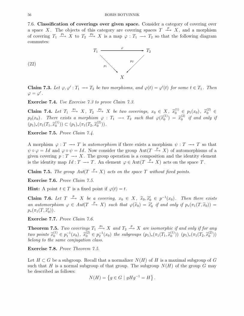
56 BORIS BOTVINNIK
7.6. Classification of coverings over given space. Consider a category of covering over
a space X . The objects of this category are covering spaces Tp−→ X , and a morphism
of covering T1p1−→ X to T2
p2−→ X is a map ϕ : T1 −→ T2 so that the following diagramcommutes:
(22)
T1
@@
@@@R
p1
T2
p2
-ϕ
X
Claim 7.3. Let ϕ, ϕ′ : T1 −→ T2 be two morphisms, and ϕ(t) = ϕ′(t) for some t ∈ T1 . Thenϕ = ϕ′ .
Exercise 7.4. Use Exercise 7.3 to prove Claim 7.3.
Claim 7.4. Let T1p1−→ X , T2
p2−→ X be two coverings, x0 ∈ X , x(1)0 ∈ p1(x0), x
(2)0 ∈
p2(x0). There exists a morphism ϕ : T1 −→ T2 such that ϕ(x(1)0 ) = x
(2)0 if and only if
(p1)∗(π1(T1, x(1)0 )) ⊂ (p1)∗(π1(T2, x
(2)0 )).
Exercise 7.5. Prove Claim 7.4.
A morphism ϕ : T −→ T is automorphism if there exists a morphism ψ : T −→ T so that
ψ ϕ = Id and ϕ ψ = Id . Now consider the group Aut(Tp−→ X) of automorphisms of a
given covering p : T −→ X . The group operation is a composition and the identity element
is the identity map Id : T −→ T . An element ϕ ∈ Aut(Tp−→ X) acts on the space T .
Claim 7.5. The group Aut(Tp−→ X) acts on the space T without fixed points.
Exercise 7.6. Prove Claim 7.5.
Hint: A point t ∈ T is a fixed point if ϕ(t) = t.
Claim 7.6. Let Tp−→ X be a covering, x0 ∈ X , x0, x
′0 ∈ p−1(x0). Then there exists
an automorphism ϕ ∈ Aut(Tp−→ X) such that ϕ(x0) = x′0 if and only if p∗(π1(T, x0)) =
p∗(π1(T, x′0)).
Exercise 7.7. Prove Claim 7.6.
Theorem 7.5. Two coverings T1p1−→ X and T2
p−→ X are isomorphic if and only if for any
two points x(1)0 ∈ p−1
1 (x0), x(2)0 ∈ p−1
2 (x0) the subgroups (p1)∗(π1(T1, x(1)0 )) (p1)∗(π1(T2, x
(2)0 ))
belong to the same conjugation class.
Exercise 7.8. Prove Theorem 7.5.
Let H ⊂ G be a subgroup. Recall that a normalizer N(H) of H is a maximal subgroup of Gsuch that H is a normal subgroup of that group. The subgroup N(H) of the group G maybe described as follows:
N(H) =g ∈ G | gHg−1 = H
.
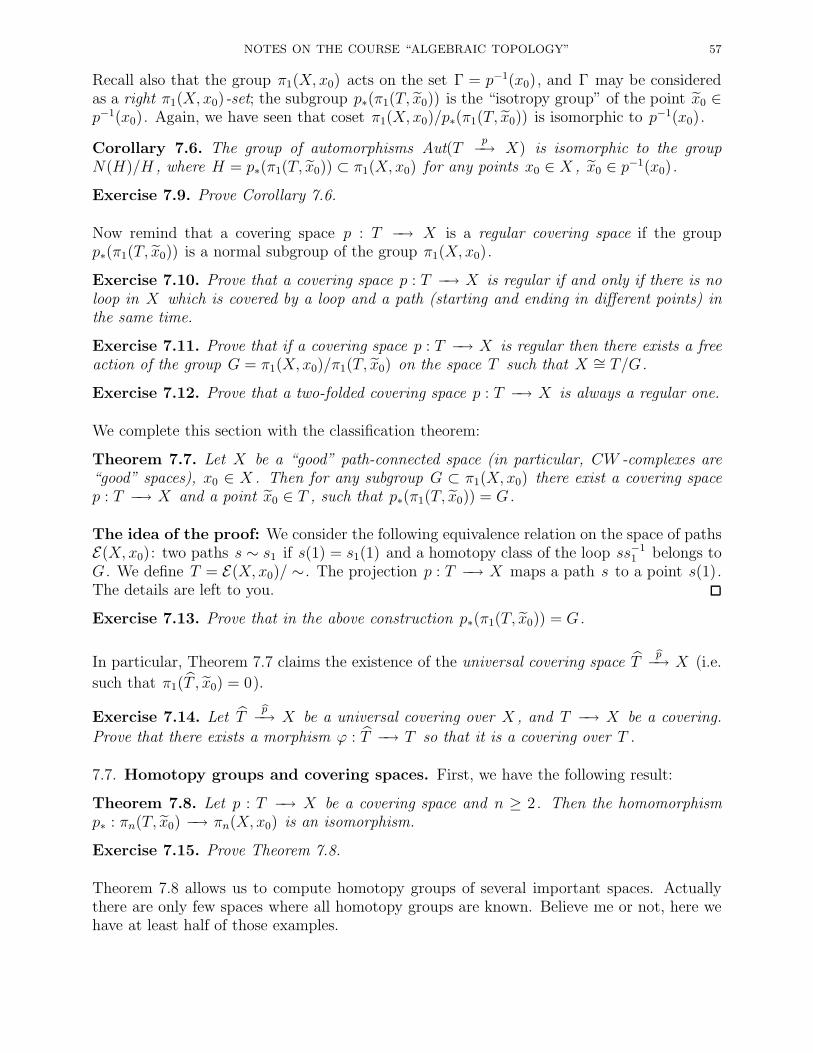
NOTES ON THE COURSE “ALGEBRAIC TOPOLOGY” 57
Recall also that the group π1(X, x0) acts on the set Γ = p−1(x0), and Γ may be consideredas a right π1(X, x0)-set; the subgroup p∗(π1(T, x0)) is the “isotropy group” of the point x0 ∈p−1(x0). Again, we have seen that coset π1(X, x0)/p∗(π1(T, x0)) is isomorphic to p−1(x0).
Corollary 7.6. The group of automorphisms Aut(Tp−→ X) is isomorphic to the group
N(H)/H , where H = p∗(π1(T, x0)) ⊂ π1(X, x0) for any points x0 ∈ X , x0 ∈ p−1(x0).
Exercise 7.9. Prove Corollary 7.6.
Now remind that a covering space p : T −→ X is a regular covering space if the groupp∗(π1(T, x0)) is a normal subgroup of the group π1(X, x0).
Exercise 7.10. Prove that a covering space p : T −→ X is regular if and only if there is noloop in X which is covered by a loop and a path (starting and ending in different points) inthe same time.
Exercise 7.11. Prove that if a covering space p : T −→ X is regular then there exists a freeaction of the group G = π1(X, x0)/π1(T, x0) on the space T such that X ∼= T/G.
Exercise 7.12. Prove that a two-folded covering space p : T −→ X is always a regular one.
We complete this section with the classification theorem:
Theorem 7.7. Let X be a “good” path-connected space (in particular, CW -complexes are“good” spaces), x0 ∈ X . Then for any subgroup G ⊂ π1(X, x0) there exist a covering spacep : T −→ X and a point x0 ∈ T , such that p∗(π1(T, x0)) = G.
The idea of the proof: We consider the following equivalence relation on the space of pathsE(X, x0): two paths s ∼ s1 if s(1) = s1(1) and a homotopy class of the loop ss−1
1 belongs toG. We define T = E(X, x0)/ ∼. The projection p : T −→ X maps a path s to a point s(1).The details are left to you.
Exercise 7.13. Prove that in the above construction p∗(π1(T, x0)) = G.
In particular, Theorem 7.7 claims the existence of the universal covering space Tbp−→ X (i.e.
such that π1(T , x0) = 0).
Exercise 7.14. Let Tbp−→ X be a universal covering over X , and T −→ X be a covering.
Prove that there exists a morphism ϕ : T −→ T so that it is a covering over T .
7.7. Homotopy groups and covering spaces. First, we have the following result:
Theorem 7.8. Let p : T −→ X be a covering space and n ≥ 2. Then the homomorphismp∗ : πn(T, x0) −→ πn(X, x0) is an isomorphism.
Exercise 7.15. Prove Theorem 7.8.
Theorem 7.8 allows us to compute homotopy groups of several important spaces. Actuallythere are only few spaces where all homotopy groups are known. Believe me or not, here wehave at least half of those examples.
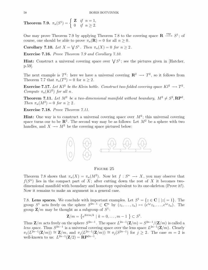
58 BORIS BOTVINNIK
Theorem 7.9. πn(S1) =
Z if n = 1,0 if n ≥ 2.
One may prove Theorem 7.9 by applying Theorem 7.8 to the covering space Rexp−−→ S1 ; of
course, one should be able to prove πn(R) = 0 for all n ≥ 0.
Corollary 7.10. Let X =∨S1 . Then πn(X) = 0 for n ≥ 2.
Exercise 7.16. Prove Theorem 7.9 and Corollary 7.10.
Hint: Construct a universal covering space over∨S1 ; see the pictures given in [Hatcher,
p.59].
The next example is T 2 : here we have a universal covering R2 −→ T 2 , so it follows fromTheorem 7.7 that πn(T
2) = 0 for n ≥ 2.
Exercise 7.17. Let Kl2 be the Klein bottle. Construct two-folded covering space Kl2 −→ T 2 .Compute πn(Kl
2) for all n.
Theorem 7.11. Let M2 be a two-dimensional manifold without boundary, M2 6= S2,RP2 .Then πn(M
2) = 0 for n ≥ 2.
Exercise 7.18. Prove Theorem 7.11.
Hint: One way is to construct a universal covering space over M2 ; this universal coveringspace turns our to be R2 . The second way may be as follows: Let M2 be a sphere with twohandles, and X −→ M2 be the covering space pictured below:
Figure 25
Theorem 7.8 shows that πn(X) = πn(M2). Now let f : Sn −→ X , you may observe that
f(Sn) lies in the compact part of X ; after cutting down the rest of X it becomes two-dimensional manifold with boundary and homotopy equivalent to its one-skeleton (Prove it!).Now it remains to make an argument in a general case.
7.8. Lens spaces. We conclude with important examples. Let S1 = z ∈ C | |z| = 1. Thegroup S1 acts freely on the sphere S2n−1 ⊂ Cn by (z1, . . . , zn) 7→ (eiϕz1, . . . , e
iϕzn). Thegroup Z/m may be thought as a subgroup of S1 :
Z/m =e2iπm/k | k = 0, . . . , m− 1
⊂ S1.
Thus Z/m acts freely on the sphere S2n−1 . The space L2n−1(Z/m) = S2n−1/(Z/m) is called alens space. Thus S2n−1 is a universal covering space over the lens space L2n−1(Z/m). Clearlyπ1(L
2n−1(Z/m)) ∼= Z/m, and πj(L2n−1(Z/m)) ∼= πj(S
2n−1) for j ≥ 2. The case m = 2 iswell-known to us: L2n−1(Z/2) = RP2n−1 .
NOTES ON THE COURSE “ALGEBRAIC TOPOLOGY” 59
Exercise 7.19. Describe a cell decomposition of the lens space L2n−1(Z/m).
Consider the sphere S3 ⊂ C2 . Let p be a prime number, and q 6= 0 mod p. We definethe lens spaces L3(p, q) as follows. We consider the action of Z/p on S3 ⊂ C2 given by theformula: T : (z1, z2) 7→ (e2πi/pz1, e
2πiq/pz2). Let L3(p, q) = S3/T .
Exercise 7.20. Prove that π1(L3(p, q)) ∼= Z/p.
Certainly the lens spaces L3(p, q) are 3-dimensional manifolds, and for given p they all havethe same fundamental group and the same higher homotopy groups πj(L
3(p, q)) for j ≥ 2since S3 is a universal covering space for all of them. Clearly one may suspect that some ofthese spaces are homeomorphic or at least homotopy equivalent. The following theorem givesclassification of the lens spaces L3(p, q) up to homotopy equivalence. The result is rathersurprising.
Theorem 7.12. The lens spaces L3(p, q) and L3(p, q′) are homotopy equivalent if and onlyif q′ ≡ ±kq mod p for some integer k .
We are not ready to prove Theorem 7.12. For instance the lenses L3(5, 1) and L3(5, 2) arenot homotopy equivalent, and L3(7, 1) and L3(7, 2) are homotopy equivalent. However it isknown that the lenses L3(7, 1) and L3(7, 2) are not homeomorphic, and the classification ofthe lenses L3(p, q) is completely resolved.

60 BORIS BOTVINNIK
8. Higher homotopy groups
8.1. More about homotopy groups. Let X be a space with a base point x0 ∈ X . Wehave defined the homotopy groups πn(X, x0) for all n ≥ 1 and even noticed that the groupsπn(X, x0) are commutative for n ≥ 2 (see the begining of Section 6). Now it is a good timeto give more details. First we have defined πn(X, x0) = [(Sn, s0), (X, x0)], where s0 ∈ Sn isa based point. Alternatively an element α ∈ πn(X, x0) could be represented by a map
f : (Dn, Sn−1) −→ (X, x0) or a map
f : (In, ∂In) −→ (X, x0).
We already defined the group operation in πn(X, x0), where the unit element is representedmy constant map Sn −→ x0 ⊂ X . It is convenient to construct a canonical inverse −α forany element α ∈ πn(X, x0). Let f ∈ α be a map
f : (Dn, Sn−1) −→ (X, x0)
representing α . We construct the map (−f) : (Dn, Sn−1) −→ (X, x0) as follows. Considerthe sphere Sn = Dn
+ ∪Sn−1 Dn− , where the hemisphere Dn
+ is identified with the above diskDn , as a domain of the map f , see Fig. 26.
Dn−
Dn+ f
τ
Figure 26
Let τ : Sn −→ Sn be a map which is identical on Dn+ and which maps Dn
− to Dn+ by the
formula (x1, . . . , xn+1) 7→ (x1, . . . ,−xn+1). Then −f = f τ : Dn− −→ X .
Exercise 8.1. Prove that the map f+(−f) : Sn −→ X is null-homotopic. Hint: It is enoughto show that the map f + (−f) : Sn −→ X exends to a map g : Dn+1 −→ X .
Exercise 8.2. Prove that πn(X × Y, x0 × y0) ∼= πn(X, x0)× πn(Y, y0). Compute πn(Tk) for
all n and k .
8.2. Dependence on the base point. Let X be a path-connected space, and x0, x1 ∈ Xbe two different points. Choose a path γ : I −→ X so that γ(0) = x0 and γ(1) = x1 . Wedefine a homomorphism
γ# : πn(X, x0) −→ πn(X, x1)
as follows. Consider the sphere Sn with a base point s0 ∈ Sn and the map ω : Sn −→ Sn ∨ I(Fig 8.2 below shows how to construct the map ω ). Indeed, the map ω takes the base points0 ∈ Sn to the point 1 ∈ I ⊂ Sn ∨ I . Then for any map f : (Sn, s0) −→ (X, x0) we defineγ#(f) to be the composition
γ#(f) : Snω−→ Sn ∨ I f∨γ−−→ X,
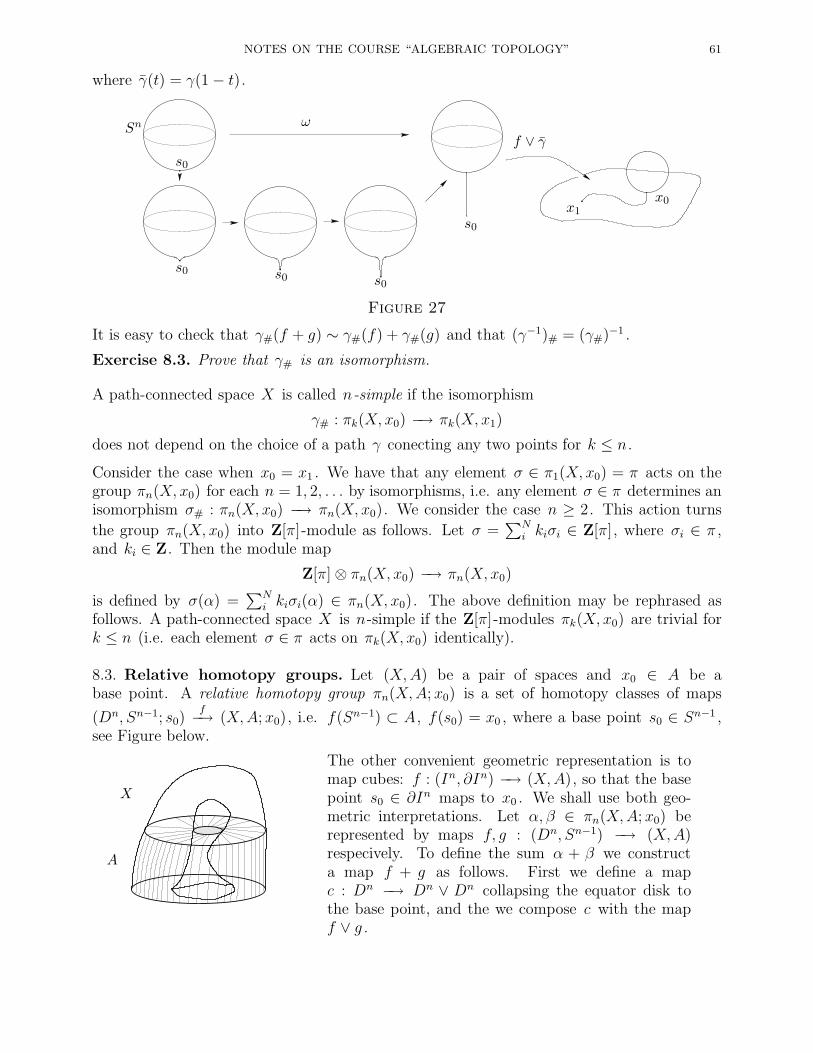
NOTES ON THE COURSE “ALGEBRAIC TOPOLOGY” 61
where γ(t) = γ(1− t).
Sn ω
s0
s0 s0 s0
s0
f ∨ γ
x1x0
Figure 27
It is easy to check that γ#(f + g) ∼ γ#(f) + γ#(g) and that (γ−1)# = (γ#)−1 .
Exercise 8.3. Prove that γ# is an isomorphism.
A path-connected space X is called n-simple if the isomorphism
γ# : πk(X, x0) −→ πk(X, x1)
does not depend on the choice of a path γ conecting any two points for k ≤ n.
Consider the case when x0 = x1 . We have that any element σ ∈ π1(X, x0) = π acts on thegroup πn(X, x0) for each n = 1, 2, . . . by isomorphisms, i.e. any element σ ∈ π determines anisomorphism σ# : πn(X, x0) −→ πn(X, x0). We consider the case n ≥ 2. This action turns
the group πn(X, x0) into Z[π]-module as follows. Let σ =∑N
i kiσi ∈ Z[π], where σi ∈ π ,and ki ∈ Z. Then the module map
Z[π]⊗ πn(X, x0) −→ πn(X, x0)
is defined by σ(α) =∑N
i kiσi(α) ∈ πn(X, x0). The above definition may be rephrased asfollows. A path-connected space X is n-simple if the Z[π]-modules πk(X, x0) are trivial fork ≤ n (i.e. each element σ ∈ π acts on πk(X, x0) identically).
8.3. Relative homotopy groups. Let (X,A) be a pair of spaces and x0 ∈ A be abase point. A relative homotopy group πn(X,A; x0) is a set of homotopy classes of maps
(Dn, Sn−1; s0)f−→ (X,A; x0), i.e. f(Sn−1) ⊂ A, f(s0) = x0 , where a base point s0 ∈ Sn−1 ,
see Figure below.
X
A
The other convenient geometric representation is tomap cubes: f : (In, ∂In) −→ (X,A), so that the basepoint s0 ∈ ∂In maps to x0 . We shall use both geo-metric interpretations. Let α, β ∈ πn(X,A; x0) berepresented by maps f, g : (Dn, Sn−1) −→ (X,A)respecively. To define the sum α + β we constructa map f + g as follows. First we define a mapc : Dn −→ Dn ∨ Dn collapsing the equator disk tothe base point, and the we compose c with the mapf ∨ g .
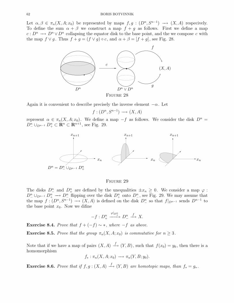
62 BORIS BOTVINNIK
Let α, β ∈ πn(X,A; x0) be represented by maps f, g : (Dn, Sn−1) −→ (X,A) respecively.To define the sum α + β we construct a map f + g as follows. First we define a mapc : Dn −→ Dn∨Dn collapsing the equator disk to the base point, and the we compose c withthe map f ∨ g . Thus f + g = (f ∨ g) c, and α+ β = [f + g], see Fig. 28.
(X,A)
f
g
c
Dn Dn ∨Dn
Figure 28
Again it is convenient to describe precisely the inverse element −α . Let
f : (Dn, Sn−1) −→ (X,A)
represent α ∈ πn(X,A; x0). We define a map −f as follows. We consider the disk Dn =Dn
− ∪Dn−1 Dn+ ⊂ Rn ⊂ Rn+1 , see Fig. 29.
Dn = Dn− ∪Dn−1 Dn
+
xn+1
xn
xn+1
xn
xn+1
xn
Figure 29
The disks Dn− and Dn
+ are defined by the unequalities ±xn ≥ 0. We consider a map ϕ :Dn
− ∪Dn−1 Dn+ −→ Dn
− flipping over the disk Dn+ onto Dn
− , see Fig. 29. We may assume thatthe map f : (Dn, Sn−1) −→ (X,A) is defined on the disk Dn
− so that f |Dn−1 sends Dn−1 tothe base point x0 . Now we difine
−f : Dn+
ϕ|Dn+−−−→ Dn
−f−→ X.
Exercise 8.4. Prove that f + (−f) ∼ ∗, where −f as above.
Exercise 8.5. Prove that the group πn(X,A; x0) is commutative for n ≥ 3.
Note that if we have a map of pairs (X,A)f−→ (Y,B), such that f(x0) = y0 , then there is a
homomorphismf∗ : πn(X,A; x0) −→ πn(Y,B; y0).
Exercise 8.6. Prove that if f, g : (X,A)f−→ (Y,B) are homotopic maps, than f∗ = g∗ .
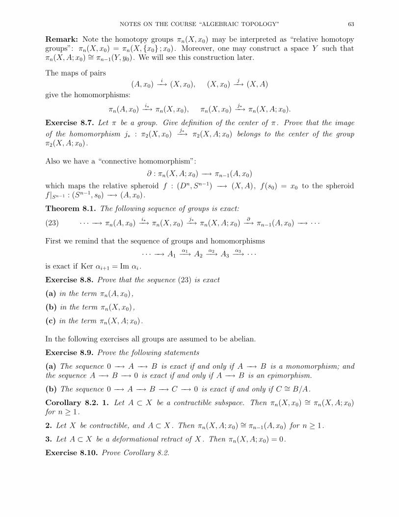
NOTES ON THE COURSE “ALGEBRAIC TOPOLOGY” 63
Remark: Note the homotopy groups πn(X, x0) may be interpreted as “relative homotopygroups”: πn(X, x0) = πn(X, x0 ; x0). Moreover, one may construct a space Y such thatπn(X,A; x0) ∼= πn−1(Y, y0). We will see this construction later.
The maps of pairs
(A, x0)i−→ (X, x0), (X, x0)
j−→ (X,A)
give the homomorphisms:
πn(A, x0)i∗−→ πn(X, x0), πn(X, x0)
j∗−→ πn(X,A; x0).
Exercise 8.7. Let π be a group. Give definition of the center of π . Prove that the image
of the homomorphism j∗ : π2(X, x0)j∗−→ π2(X,A; x0) belongs to the center of the group
π2(X,A; x0).
Also we have a “connective homomorphism”:
∂ : πn(X,A; x0) −→ πn−1(A, x0)
which maps the relative spheroid f : (Dn, Sn−1) −→ (X,A), f(s0) = x0 to the spheroidf |Sn−1 : (Sn−1, s0) −→ (A, x0).
Theorem 8.1. The following sequence of groups is exact:
(23) · · · −→ πn(A, x0)i∗−→ πn(X, x0)
j∗−→ πn(X,A; x0)∂−→ πn−1(A, x0) −→ · · ·
First we remind that the sequence of groups and homomorphisms
· · · −→ A1α1−→ A2
α2−→ A3α3−→ · · ·
is exact if Ker αi+1 = Im αi .
Exercise 8.8. Prove that the sequence (23) is exact
(a) in the term πn(A, x0),
(b) in the term πn(X, x0),
(c) in the term πn(X,A; x0).
In the following exercises all groups are assumed to be abelian.
Exercise 8.9. Prove the following statements
(a) The sequence 0 −→ A −→ B is exact if and only if A −→ B is a monomorphism; andthe sequence A −→ B −→ 0 is exact if and only if A −→ B is an epimorphism.
(b) The sequence 0 −→ A −→ B −→ C −→ 0 is exact if and only if C ∼= B/A.
Corollary 8.2. 1. Let A ⊂ X be a contractible subspace. Then πn(X, x0) ∼= πn(X,A; x0)for n ≥ 1.
2. Let X be contractible, and A ⊂ X . Then πn(X,A; x0) ∼= πn−1(A, x0) for n ≥ 1.
3. Let A ⊂ X be a deformational retract of X . Then πn(X,A; x0) = 0.
Exercise 8.10. Prove Corollary 8.2.
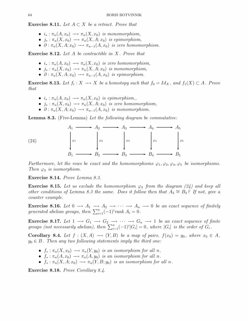
64 BORIS BOTVINNIK
Exercise 8.11. Let A ⊂ X be a retract. Prove that
• i∗ : πn(A, x0) −→ πn(X, x0) is monomorphism,• j∗ : πn(X, x0) −→ πn(X,A; x0) is epimorphism,• ∂ : πn(X,A; x0) −→ πn−1(A, x0) is zero homomorphism.
Exercise 8.12. Let A be contractible in X . Prove that
• i∗ : πn(A, x0) −→ πn(X, x0) is zero homomorphism,• j∗ : πn(X, x0) −→ πn(X,A; x0) is monomorphism,• ∂ : πn(X,A; x0) −→ πn−1(A, x0) is epimorphism.
Exercise 8.13. Let ft : X −→ X be a homotopy such that f0 = IdX , and f1(X) ⊂ A. Provethat
• i∗ : πn(A, x0) −→ πn(X, x0) is epimorphism.,• j∗ : πn(X, x0) −→ πn(X,A; x0) is zero homomorphism,• ∂ : πn(X,A; x0) −→ πn−1(A, x0) is monomorphism.
Lemma 8.3. (Five-Lemma) Let the following diagram be commutative:
(24)
A1
?
ϕ1
A2
?
ϕ2
A3
?
ϕ3
A4
?
ϕ4
A5
?
ϕ5
- - - -
B1 B2 B3 B4 B5- - - -
Furthermore, let the rows be exact and the homomorphisms ϕ1, ϕ2, ϕ4, ϕ5 be isomorphisms.Then ϕ3 is isomorphism.
Exercise 8.14. Prove Lemma 8.3.
Exercise 8.15. Let us exclude the homomorphism ϕ3 from the diagram (24) and keep allother conditions of Lemma 8.3 the same. Does it follow then that A3
∼= B3? If not, give acounter example.
Exercise 8.16. Let 0 −→ A1 −→ A2 −→ · · · −→ An −→ 0 be an exact sequence of finitelygenerated abelian groups, then
∑ni=1(−1)irank Ai = 0.
Exercise 8.17. Let 1 −→ G1 −→ G2 −→ · · · −→ Gn −→ 1 be an exact sequence of finitegroups (not necessarily abelian), then
∑ni=1(−1)i|Gi| = 0, where |Gi| is the order of Gi .
Corollary 8.4. Let f : (X,A) −→ (Y,B) be a map of pairs, f(x0) = y0 , where x0 ∈ A,y0 ∈ B . Then any two following statements imply the third one:
• f∗ : πn(X, x0) −→ πn(Y, y0) is an isomorphism for all n.• f∗ : πn(A, x0) −→ πn(A, y0) is an isomorphism for all n.• f∗ : πn(X,A; x0) −→ πn(Y,B; y0) is an isomorphism for all n.
Exercise 8.18. Prove Corollary 8.4.

NOTES ON THE COURSE “ALGEBRAIC TOPOLOGY” 65
9. Fiber bundles
9.1. First steps toward fiber bundles. Covering spaces may be considered as a perfecttool to study the fundamental group. Fiber bundles provide the same kind of tool to studythe higher homotopy groups, as we shall see soon.
Definition 9.1. A locally trivial fiber bundle is a four-tuple (E,B, F, p), where E,B, F arespaces, and p : E −→ B is a map with the following property:
• For each point x ∈ B there exists a neighborhood U of x such that p−1(U) is home-omorphic to U × F , moreover the homeomorphism ϕU : p−1(U) −→ U × F shouldmake the diagram
p−1(U)
@@
@@@R
p
U × F
pr
-ϕU
U
commute. Here pr : U × F −→ U is a projection on the first factor.
The spaces E,B, F have their special names: E is a total space, B is a base, and F is afiber. The inverse image Fx ∼= p−1(x) is clearly homeomorphic to the fiber F for each pointx ∈ B . However, these homemorphisms depend on x. As in the case of covering spaces, thefollowing commutative diagram
E1
@@
@@@R
p1
E2
p2
-f
B
gives a morphism of fiber bundles (E1, B, F1, p1) to (E2, B, F2, p2). Two fiber bundles(E1, B, F1, p1) and (E2, B, F2, p2) are equivalent if there exist morphisms
f : (E1, B, F1, p1) −→ (E2, B, F2, p2), g : (E2, B, F2, p2) −→ (E1, B, F1, p1)
such that f g = Id and g f = Id . In particular, a fiber bundle p : E −→ B is trivial if itis equivalent to the bundle B × F −→ B :
E
@@
@@@R
p
B × F
pr
-f
B
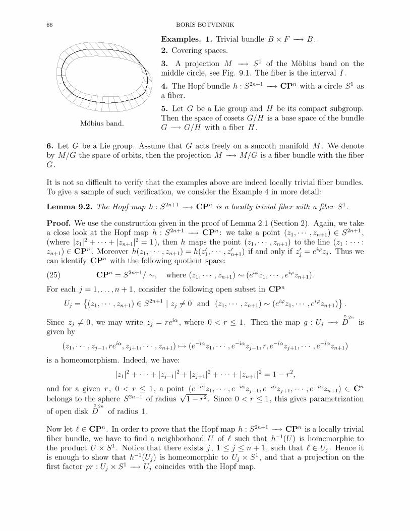
66 BORIS BOTVINNIK
Mobius band.
Examples. 1. Trivial bundle B × F −→ B .
2. Covering spaces.
3. A projection M −→ S1 of the Mobius band on themiddle circle, see Fig. 9.1. The fiber is the interval I .
4. The Hopf bundle h : S2n+1 −→ CPn with a circle S1 asa fiber.
5. Let G be a Lie group and H be its compact subgroup.Then the space of cosets G/H is a base space of the bundleG −→ G/H with a fiber H .
6. Let G be a Lie group. Assume that G acts freely on a smooth manifold M . We denoteby M/G the space of orbits, then the projection M −→ M/G is a fiber bundle with the fiberG.
It is not so difficult to verify that the examples above are indeed locally trivial fiber bundles.To give a sample of such verification, we consider the Example 4 in more detail:
Lemma 9.2. The Hopf map h : S2n+1 −→ CPn is a locally trivial fiber with a fiber S1 .
Proof. We use the construction given in the proof of Lemma 2.1 (Section 2). Again, we takea close look at the Hopf map h : S2n+1 −→ CPn : we take a point (z1, · · · , zn+1) ∈ S2n+1 ,(where |z1|2 + · · ·+ |zn+1|2 = 1), then h maps the point (z1, · · · , zn+1) to the line (z1 : · · · :zn+1) ∈ CPn . Moreover h(z1, · · · , zn+1) = h(z′1, · · · , z′n+1) if and only if z′j = eiϕzj . Thus wecan identify CPn with the following quotient space:
(25) CPn = S2n+1/ ∼, where (z1, · · · , zn+1) ∼ (eiϕz1, · · · , eiϕzn+1).
For each j = 1, . . . , n+ 1, consider the following open subset in CPn
Uj =(z1, · · · , zn+1) ∈ S2n+1 | zj 6= 0 and (z1, · · · , zn+1) ∼ (eiϕz1, · · · , eiϕzn+1)
.
Since zj 6= 0, we may write zj = reiα , where 0 < r ≤ 1. Then the map g : Uj −→D
2n
isgiven by
(z1, · · · , zj−1, reiα, zj+1, · · · , zn+1) 7→ (e−iαz1, · · · , e−iαzj−1, r, e
−iαzj+1, · · · , e−iαzn+1)
is a homeomorphism. Indeed, we have:
|z1|2 + · · ·+ |zj−1|2 + |zj+1|2 + · · ·+ |zn+1|2 = 1− r2,
and for a given r , 0 < r ≤ 1, a point (e−iαz1, · · · , e−iαzj−1, e−iαzj+1, · · · , e−iαzn+1) ∈ Cn
belongs to the sphere S2n−1 of radius√
1− r2 . Since 0 < r ≤ 1, this gives parametrization
of open diskD
2n
of radius 1.
Now let ℓ ∈ CPn . In order to prove that the Hopf map h : S2n+1 −→ CPn is a locally trivialfiber bundle, we have to find a neighborhood U of ℓ such that h−1(U) is homemorphic tothe product U × S1 . Notice that there exists j , 1 ≤ j ≤ n + 1, such that ℓ ∈ Uj . Hence itis enough to show that h−1(Uj) is homeomorphic to Uj × S1 , and that a projection on thefirst factor pr : Uj × S1 −→ Uj coincides with the Hopf map.

NOTES ON THE COURSE “ALGEBRAIC TOPOLOGY” 67
Now we see that h−1(Uj) ⊂ S2n+1 is given as
h−1(Uj) = (z1, · · · , zn+1) ∈ S2n+1 | zj = reiα 6= 0
∼= ((e−iαz1, · · · , e−iαzj−1, r, e−iαzj+1, · · · , e−iαzn+1), e
−iα) = Uj × S1.
Clearly the projection on the first factor coincides with the Hopf map.
Exercise 9.1. Prove that the Hopf map S4n+3 −→ HPn is locally trivial fiber bundle.
Exercise 9.2. Here we specify the example 5. Note that Sp(1) = S3 , and S1 is a subgroupof Sp(1). Prove that the fiber bundle Sp(1) −→ Sp(1)/S1 is equivalent to the Hopf bundleS3 −→ CP1 .8
Exercise 9.3. Here we specify the example 6. Let S2n+1 be a unit sphere in Cn+1 ,S2n+1 = |z1|2 + . . .+ |zn+1| = 1|. The group S1 = eiϕ acts on S2n+1 by the formula(z1, . . . , zn+1) −→ (eiϕz1, . . . , e
iϕzn+1). Prove that this action is free, and that a fiber bundleS2n+1 −→ S2n+1/S1 is equivalent to the Hopf bundle S2n+1 −→ CPn .
Exercise 9.4. Let f : M −→ N be a smooth map, where M , N are smooth manifolds.Assume that the map f is a submersion, i.e. f is onto and the differential dfx : TMx −→TMf(x) is an epimorphism for any x ∈M . Prove that (M,N, f−1(x), f) is a locally-trivialfiber bundle.
Exercise 9.5. Prove that the fiber bundles from the examples 3–6 are nontrivial fiber bundles.
9.2. Constructions of new fiber bundles. There are two important ways to constructnew fiber bundles.
1. Restriction. Let Ep−→ B be a fiber bundle with a fiber F , and let B′ ⊂ B be a subset.
Let E ′ = p−1(B′). The bundle E ′ p′−→ B′ , where p′ = p|E′ is a restriction of the bundle
Ep−→ B on the subspace B′ ⊂ B .
2. Induced fiber bundle. Let Ep−→ B be a fiber bundle with a fiber F , and X
f−→ B bea map. Let f ∗(E) ⊂ X ×E be the following subspace:
f ∗(E) = (x, e) ∈ X ×E | f(x) = p(e) .
There are two natural maps: f ∗(E)f∗−→ E (where f ∗(x, e) = e) and f ∗(E)
p′−→ X (where
p′(x, e) = x). It is easy to check that the map f ∗(E)p′−→ X is a locally–trivial bundle over
X with the same fiber F and that the diagram
f ∗(E)
?
p′
E
?
p
-f∗
X B-f
commutes. The bundle f ∗(E)p′−→ X is called induced fiber bundle.
8 It may be helpfull to remember that Sp(1) is the set of all unit quaternions α = α1 + iα2 + jα3 +kα4 ∈Sp(1), and S1 = α1 + iα2 .
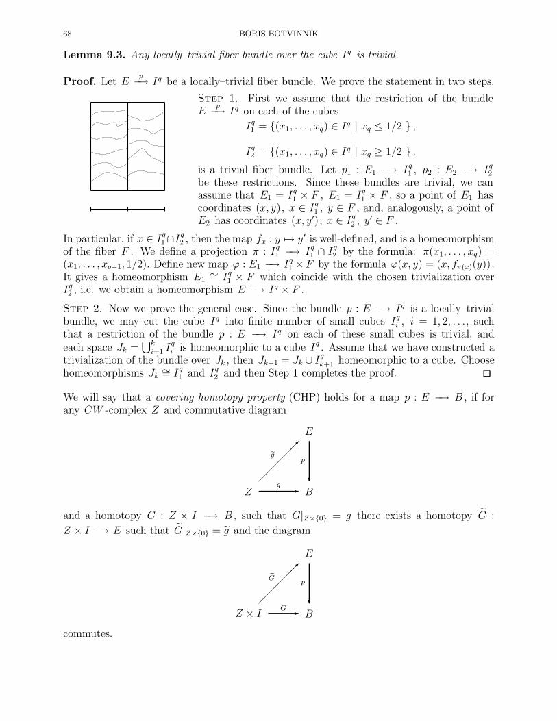
68 BORIS BOTVINNIK
Lemma 9.3. Any locally–trivial fiber bundle over the cube Iq is trivial.
Proof. Let Ep−→ Iq be a locally–trivial fiber bundle. We prove the statement in two steps.
Step 1. First we assume that the restriction of the bundleE
p−→ Iq on each of the cubes
Iq1 = (x1, . . . , xq) ∈ Iq | xq ≤ 1/2 ,
Iq2 = (x1, . . . , xq) ∈ Iq | xq ≥ 1/2 .is a trivial fiber bundle. Let p1 : E1 −→ Iq1 , p2 : E2 −→ Iq2be these restrictions. Since these bundles are trivial, we canassume that E1 = Iq1 × F , E1 = Iq1 × F , so a point of E1 hascoordinates (x, y), x ∈ Iq1 , y ∈ F , and, analogously, a point ofE2 has coordinates (x, y′), x ∈ Iq2 , y′ ∈ F .
In particular, if x ∈ Iq1∩Iq2 , then the map fx : y 7→ y′ is well-defined, and is a homeomorphismof the fiber F . We define a projection π : Iq1 −→ Iq1 ∩ Iq2 by the formula: π(x1, . . . , xq) =(x1, . . . , xq−1, 1/2). Define new map ϕ : E1 −→ Iq1 ×F by the formula ϕ(x, y) = (x, fπ(x)(y)).It gives a homeomorphism E1
∼= Iq1 × F which coincide with the chosen trivialization overIq2 , i.e. we obtain a homeomorphism E −→ Iq × F .
Step 2. Now we prove the general case. Since the bundle p : E −→ Iq is a locally–trivialbundle, we may cut the cube Iq into finite number of small cubes Iqi , i = 1, 2, . . ., suchthat a restriction of the bundle p : E −→ Iq on each of these small cubes is trivial, andeach space Jk =
⋃ki=1 I
qi is homeomorphic to a cube Iq1 . Assume that we have constructed a
trivialization of the bundle over Jk , then Jk+1 = Jk ∪ Iqk+1 homeomorphic to a cube. Choosehomeomorphisms Jk ∼= Iq1 and Iq2 and then Step 1 completes the proof.
We will say that a covering homotopy property (CHP) holds for a map p : E −→ B , if forany CW -complex Z and commutative diagram
E
?
p
Z
eg
B-g
and a homotopy G : Z × I −→ B , such that G|Z×0 = g there exists a homotopy G :
Z × I −→ E such that G|Z×0 = g and the diagram
E
?
p
Z × I
eG
B-G
commutes.

NOTES ON THE COURSE “ALGEBRAIC TOPOLOGY” 69
Theorem 9.4. (Theorem on Covering Homotopy) The covering homotopy propertyholds for a locally-trivial fiber bundle E −→ B .
We will prove a stronger version of Theorem 9.4, namely we assume in addition the following.
• There is a subcomplex Z ′ ⊂ Z and a homotopy G′ : Z ′ × I −→ E covering thehomotopy G|Z′×I .
Proof. Case 1. Let the fiber bundle p : E −→ B be trivial, and Z be any CW -complex. Weidentify E ∼= B×F , and maps to B×F with the pairs of maps to B and F . Then the mapg : Z −→ E = B × F is given by a pair g = (g, h), where g : Z −→ B is the above map, and
h : Z −→ F be some continuous map. The homotopy G′ : Z ′ × I −→ E is given by the pair
G′ = (G′, H ′), where G′ = G|Z′×I : Z ′ × I −→ B is determined by the homotopy G and andthe homotopy H ′ : Z ′ × I −→ F is such that H ′|Z′×0 = h|Z′ . Thus the Borsuk Theoremgives us that there exists a homotopy H : Z × I −→ F extending the map h : Z −→ F andthe homotopy H ′ : Z ′ × I −→ F . The covering homotopy G : Z × I −→ B × F = E is
defined by G(z, t) = (G(z, t), H(z, t)).
Case 2. The fiber bundle p : E −→ B is arbitrary, Z = Dn , Z ′ = Sn−1 . Let g : Dn −→ B ,
g′ : Sn−1 −→ B , f : Dn −→ E , g′ : Sn−1 −→ E , and G : Dn × I −→ B , G′ : Sn−1 × I −→ Ebe the corresponding maps and homotopies.
The map G : Dn×I −→ B induces the bundle G∗(E) −→ Dn×I , which is trivial by Lemma9.3. Recall that the total space
G∗(E) = ((x, t), e) | G(x, t) = p(e) ⊂ (Dn × I)× E.
Let G∗ : G∗(E) −→ E be a natural map (projection). We define a map h : Dn −→ G∗(E) by
h(x) = ((x, 0), g(x)). This map is well-defined since G(x, 0) = g(x) = p g(x) and h coversthe map h : Dn −→ Dn× I given by x 7→ (x, 0). The homotopy H : Dn× I −→ Dn× I (the
identity map!), and H ′ : Sn−1 × I −→ G∗(E), where H ′(x, t) = ((x, t), G′(x, t)) satisfy theconditions of the theorem. Indeed, we have the commutative diagrams:
(26)
G∗(E)
?
p′
Sn−1 Dn
eh
Dn × I- -h
G∗(E)
?
p′
Sn−1 × I*
eH′
D × I
eH
Dn × I- -H=Id
The map H from (26) exists be the Case 1. Thus the map G = G∗ H : Dn× I −→ E coversthe homotopy G : Dn × I −→ B as required.
Case 3. Now the fiber bundle Ep−→ B is arbitrary, and the CW -complex Z is finite. By
induction, we may assume that the difference Z \ Z ′ is a single cell en . Let Φ : Dn −→ Zbe a corresponding characteristic map, and ϕ = Φ|Sn−1 be an attaching map. Then the map
h = g Φ : Dn −→ E and the homotopies
H = G (Φ× Id) : Dn × I −→ B,
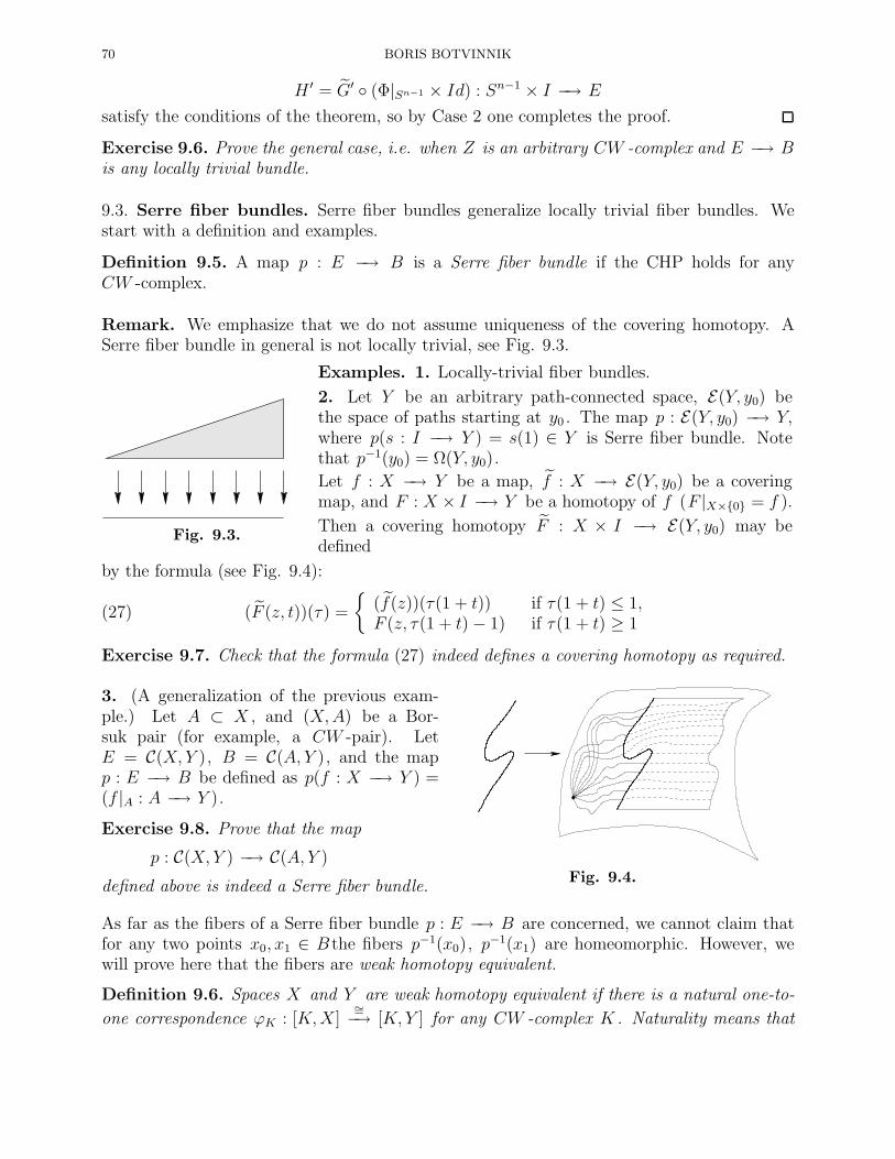
70 BORIS BOTVINNIK
H ′ = G′ (Φ|Sn−1 × Id) : Sn−1 × I −→ E
satisfy the conditions of the theorem, so by Case 2 one completes the proof.
Exercise 9.6. Prove the general case, i.e. when Z is an arbitrary CW -complex and E −→ Bis any locally trivial bundle.
9.3. Serre fiber bundles. Serre fiber bundles generalize locally trivial fiber bundles. Westart with a definition and examples.
Definition 9.5. A map p : E −→ B is a Serre fiber bundle if the CHP holds for anyCW -complex.
Remark. We emphasize that we do not assume uniqueness of the covering homotopy. ASerre fiber bundle in general is not locally trivial, see Fig. 9.3.
Fig. 9.3.
Examples. 1. Locally-trivial fiber bundles.
2. Let Y be an arbitrary path-connected space, E(Y, y0) bethe space of paths starting at y0 . The map p : E(Y, y0) −→ Y,where p(s : I −→ Y ) = s(1) ∈ Y is Serre fiber bundle. Notethat p−1(y0) = Ω(Y, y0).
Let f : X −→ Y be a map, f : X −→ E(Y, y0) be a coveringmap, and F : X × I −→ Y be a homotopy of f (F |X×0 = f ).
Then a covering homotopy F : X × I −→ E(Y, y0) may bedefined
by the formula (see Fig. 9.4):
(27) (F (z, t))(τ) =
(f(z))(τ(1 + t)) if τ(1 + t) ≤ 1,F (z, τ(1 + t)− 1) if τ(1 + t) ≥ 1
Exercise 9.7. Check that the formula (27) indeed defines a covering homotopy as required.
3. (A generalization of the previous exam-ple.) Let A ⊂ X , and (X,A) be a Bor-suk pair (for example, a CW -pair). LetE = C(X, Y ), B = C(A, Y ), and the mapp : E −→ B be defined as p(f : X −→ Y ) =(f |A : A −→ Y ).
Exercise 9.8. Prove that the map
p : C(X, Y ) −→ C(A, Y )
defined above is indeed a Serre fiber bundle.Fig. 9.4.
As far as the fibers of a Serre fiber bundle p : E −→ B are concerned, we cannot claim thatfor any two points x0, x1 ∈ B the fibers p−1(x0), p
−1(x1) are homeomorphic. However, wewill prove here that the fibers are weak homotopy equivalent.
Definition 9.6. Spaces X and Y are weak homotopy equivalent if there is a natural one-to-
one correspondence ϕK : [K,X]∼=−→ [K, Y ] for any CW -complex K . Naturality means that
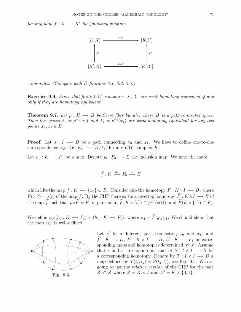
NOTES ON THE COURSE “ALGEBRAIC TOPOLOGY” 71
for any map f : K −→ K ′ the following diagram
[K,X] [K,Y ]-ϕK
[K ′,X]
6
f∗
[K ′, Y ]
6
f∗
-ϕK ′
commutes. (Compare with Definitions 3.1, 3.2, 3.3.)
Exercise 9.9. Prove that finite CW -complexes X , Y are weak homotopy equivalent if andonly if they are homotopy equivalent.
Theorem 9.7. Let p : E −→ B be Serre fiber bundle, where B is a path-connected space.Then the spaces F0 = p−1(x0) and F1 = p−1(x1) are weak homotopy equivalent for any twopoints x0, x1 ∈ B .
Proof. Let s : I −→ B be a path connecting x0 and x1 . We have to define one-to-onecorrespondence ϕK : [K,F0] −→ [K,F1] for any CW -complex K .
Let h0 : K −→ F0 be a map. Denote i0 : F0 −→ E the inclusion map. We have the map:
f : Kh0−→ F0
i0−→ E
which lifts the map f : K −→ x0 ⊂ B . Consider also the homotopy F : K×I −→ B , where
F (x, t) = s(t) of the map f . By the CHP there exists a covering homotopy F : K×I −→ E of
the map f such that pF = F , in particular, F (K×t) ⊂ p−1(s(t)), and F (K×1) ⊂ F1 .
We define ϕK(h0 : K −→ F0) = (h1 : K −→ F1), where h1 = F |K×1 . We should show thatthe map ϕK is well-defined.
Fig. 9.5.
Let s′ be a different path connecting x0 and x1 , and
f ′ : K −→ E , F ′ : K × I −→ B , h′ : K −→ F1 be corre-sponding maps and homotopies determined by s′ . Assumethat s and s′ are homotopic, and let S : I × I −→ B bea corresponding homotopy. Denote by T : I × I −→ B amap defined by T (t1, t2) = S(t2, t1), see Fig. 9.5. We aregoing to use the relative version of the CHP for the pairZ ′ ⊂ Z where Z = K × I and Z ′ = K × 0, 1.
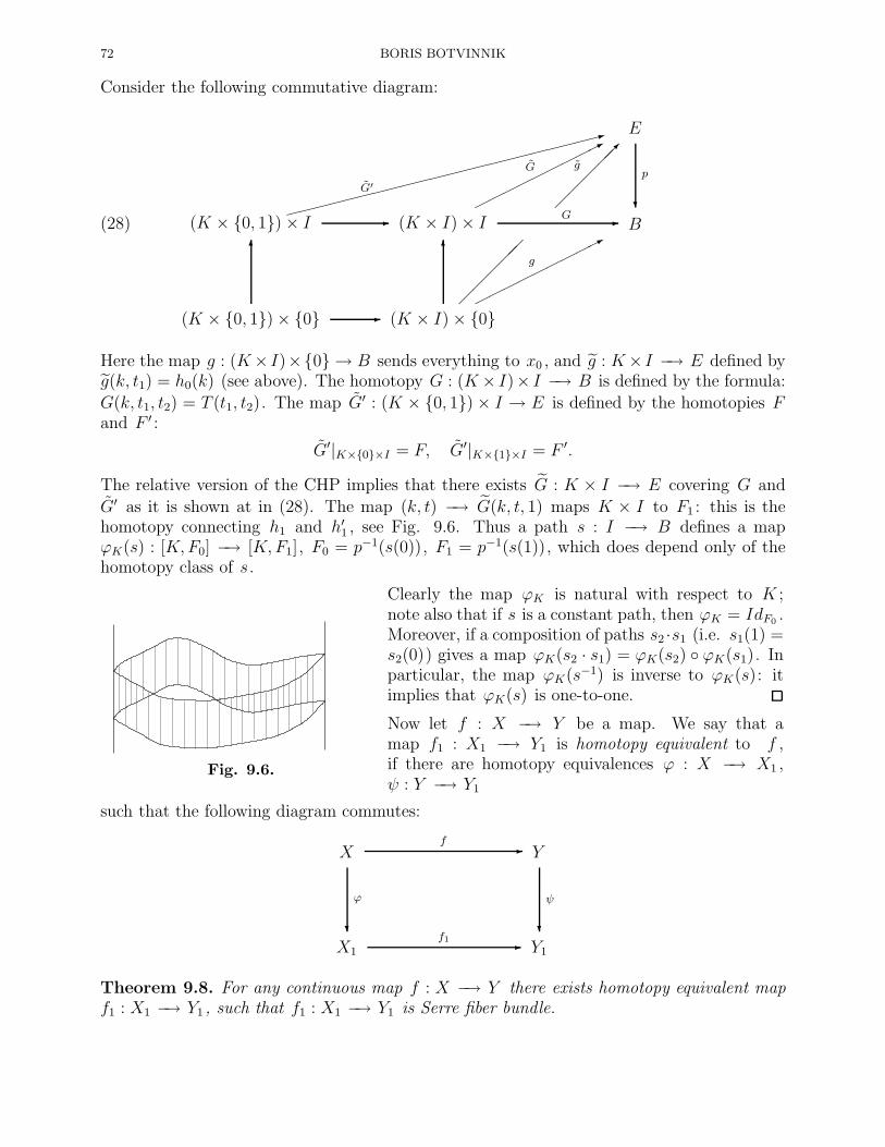
72 BORIS BOTVINNIK
Consider the following commutative diagram:
:
G′
(28)
E
?
p
(K × 0, 1)× I (K × I)× I*
G
g
B- -G
(K × 0, 1)× 0
6
(K × I)× 0
6
*g
-
Here the map g : (K× I)×0 → B sends everything to x0 , and g : K× I −→ E defined byg(k, t1) = h0(k) (see above). The homotopy G : (K× I)× I −→ B is defined by the formula:
G(k, t1, t2) = T (t1, t2). The map G′ : (K × 0, 1)× I → E is defined by the homotopies Fand F ′ :
G′|K×0×I = F, G′|K×1×I = F ′.
The relative version of the CHP implies that there exists G : K × I −→ E covering G and
G′ as it is shown at in (28). The map (k, t) −→ G(k, t, 1) maps K × I to F1 : this is thehomotopy connecting h1 and h′1 , see Fig. 9.6. Thus a path s : I −→ B defines a mapϕK(s) : [K,F0] −→ [K,F1], F0 = p−1(s(0)), F1 = p−1(s(1)), which does depend only of thehomotopy class of s.
Fig. 9.6.
Clearly the map ϕK is natural with respect to K ;note also that if s is a constant path, then ϕK = IdF0 .Moreover, if a composition of paths s2 ·s1 (i.e. s1(1) =s2(0)) gives a map ϕK(s2 · s1) = ϕK(s2) ϕK(s1). Inparticular, the map ϕK(s−1) is inverse to ϕK(s): itimplies that ϕK(s) is one-to-one.
Now let f : X −→ Y be a map. We say that amap f1 : X1 −→ Y1 is homotopy equivalent to f ,if there are homotopy equivalences ϕ : X −→ X1 ,ψ : Y −→ Y1
such that the following diagram commutes:
X
?
ϕ
Y
?
ψ
-f
X1 Y1-f1
Theorem 9.8. For any continuous map f : X −→ Y there exists homotopy equivalent mapf1 : X1 −→ Y1 , such that f1 : X1 −→ Y1 is Serre fiber bundle.
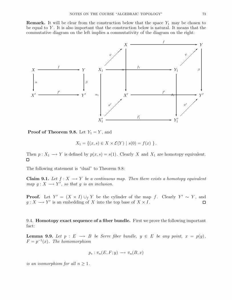
NOTES ON THE COURSE “ALGEBRAIC TOPOLOGY” 73
Remark. It will be clear from the construction below that the space Y1 may be chosen tobe equal to Y . It is also important that the construction below is natural. It means that thecommutative diagram on the left implies a commutativity of the diagram on the right:
X
?
α
Y
?
β
-f
X ′ Y ′-f ′
X
?
α
Y
?
β
-f
X1
ϕ
?
α1
Y1
ψ
?
β1
-f1
X ′ Y ′-f ′
X ′1
ϕ′
Y ′1
ψ′
-f ′1
Proof of Theorem 9.8. Let Y1 = Y , and
X1 = (x, s) ∈ X × E(Y ) | s(0) = f(x) .
Then p : X1 −→ Y is defined by p(x, s) = s(1). Clearly X and X1 are homotopy equivalent.
The following statement is “dual” to Theorem 9.8:
Claim 9.1. Let f : X −→ Y be a continuous map. Then there exists a homotopy equivalentmap g : X −→ Y ′ , so that g is an inclusion.
Proof. Let Y ′ = (X × I) ∪f Y be the cylinder of the map f . Clearly Y ′ ∼ Y , andg : X −→ Y ′ is an embedding of X into the top base of X × I .
9.4. Homotopy exact sequence of a fiber bundle. First we prove the following importantfact:
Lemma 9.9. Let p : E −→ B be Serre fiber bundle, y ∈ E be any point, x = p(y),F = p−1(x). The homomorphism
p∗ : πn(E,F ; y) −→ πn(B, x)
is an isomorphism for all n ≥ 1.

74 BORIS BOTVINNIK
ϕ1/6
ϕ2/6
ϕ3/6
ϕ4/6ϕ5/6
(b)
(a)
Fig. 9.7.
Proof. p∗ is a monomorphism. Let α ∈ πn(E,F ; y)
be represented by a map f : Dn −→ E (where f |Sn−1 :
Sn−1 −→ F , and f(s0) = y ). Then the map
f = p f : Dn −→ B
has the property that f(Sn−1) = x and [f ] = p∗(α) ∈πn(B, x). Assume α ∈ Ker p∗ , then there exists a homo-topy ft : Dn −→ B , so that f0 = f and f1(D
n) = x. Thecovering homotopy property (the strong version) implies
that there exists a homotopy ft : Dn −→ E covering thehomotopy ft . In particular f1(D
n) ⊂ F = p−1(x) since
p f1(Dn) = f1(D
n) = x.
p∗ is an epimorphism. Consider the homotopy ϕt :Sn−1 −→ Sn , so that ϕ : Sn−1×I −→ Sn , ϕ(Sn−1×I) =Sn as it is shown at Fig. 9.7 (a). Let f : Sn −→ B be amap representing β ∈ πn(B, x). Consider the homotopygt = f ϕt : Sn−1 −→ B . Then we lift the homotopy gtup to a homotopy gt : Sn−1 −→ E by applying the CHP.The homotopy gt may be considered as a map h : Dn −→E , where the disk Dn is covered by (n − 1)-spheres asit is shown, see Fig. 9.7 (b), and the map h on thesespheres is given by gt . Clearly the map h : Dn −→ E
gives a representative of an element α ∈ πn(E,F ), so that p∗(α) = β .
Now the exact sequence of the pair (E,F ; y):
· · · −→ πn(F, y)i∗−→ πn(E, y)
j∗−→ πn(E,F ; y)∂−→ πn−1(F, y) −→ · · ·
gives the exact sequence:
(29) · · · −→ πn(F, y)i∗−→ πn(E, y)
j∗−→ πn(B, x)∂−→ πn−1(F, y) −→ · · ·
We call the sequence (29) a homotopy exact sequence of Serre fibration.
Exercise 9.10. Apply the sequence (29) for the Hopf fibration S3 −→ S2 . Prove that (a)π2(S
2) = π1(S1) = Z; (b) πn(S
3) = πn(S2).
Exercise 9.11. Let S∞ −→ CP∞ be the Hopf fibration. Using the fact S∞ ∼ ∗, prove thatπn(CP∞) = 0 for n 6= 2, and π2(CP∞) = Z.
Exercise 9.12. Prove that πn(Ω(X)) ∼= πn+1(X) for any X and n ≥ 0.
Exercise 9.13. Prove that if the groups π∗(B), π∗(F ) are finite (finitely generated), thenthe groups π∗(E) are finite (finitely generated) as well.
Exercise 9.14. Assume that a fiber bundle p : E −→ B has a section, i.e. a map s : B −→ E ,such that p s = IdB . Prove the isomorphism πn(E) ∼= πn(B)⊕ πn(F ).
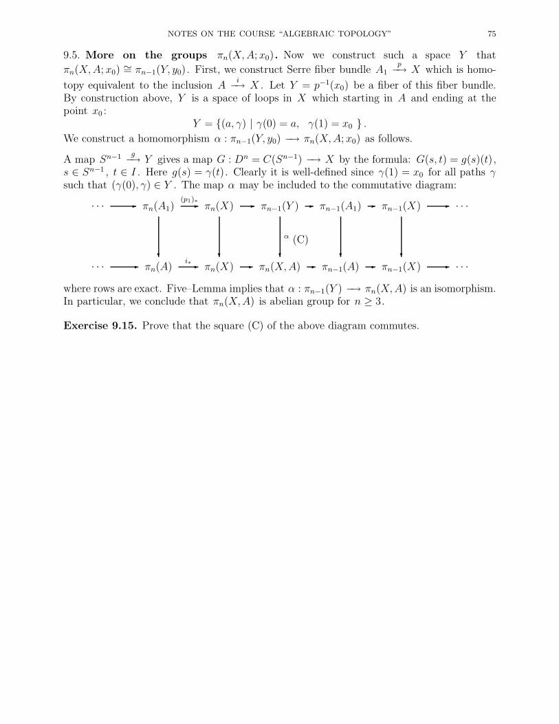
NOTES ON THE COURSE “ALGEBRAIC TOPOLOGY” 75
9.5. More on the groups πn(X,A; x0). Now we construct such a space Y that
πn(X,A; x0) ∼= πn−1(Y, y0). First, we construct Serre fiber bundle A1p−→ X which is homo-
topy equivalent to the inclusion Ai−→ X . Let Y = p−1(x0) be a fiber of this fiber bundle.
By construction above, Y is a space of loops in X which starting in A and ending at thepoint x0 :
Y = (a, γ) | γ(0) = a, γ(1) = x0 .We construct a homomorphism α : πn−1(Y, y0) −→ πn(X,A; x0) as follows.
A map Sn−1 g−→ Y gives a map G : Dn = C(Sn−1) −→ X by the formula: G(s, t) = g(s)(t),s ∈ Sn−1 , t ∈ I . Here g(s) = γ(t). Clearly it is well-defined since γ(1) = x0 for all paths γsuch that (γ(0), γ) ∈ Y . The map α may be included to the commutative diagram:
(C)
· · · πn(A1)
?
πn(X)
?
πn−1(Y )
?
α
πn−1(A1)
?
πn−1(X)
?
· · ·- -(p1)∗ - - - -
· · · πn(A) πn(X) πn(X,A) πn−1(A) πn−1(X) · · ·- -i∗ - - - -
where rows are exact. Five–Lemma implies that α : πn−1(Y ) −→ πn(X,A) is an isomorphism.In particular, we conclude that πn(X,A) is abelian group for n ≥ 3.
Exercise 9.15. Prove that the square (C) of the above diagram commutes.

76 BORIS BOTVINNIK
10. Suspension Theorem and Whitehead product
10.1. The Freudenthal Theorem. Let X be a space with a base point x0 . We constructthe homomorphism
(30) Σ : πq(X) −→ πq+1(ΣX)
as follows. Let α ∈ πq(X), and a map f : Sq −→ X be a representative of α . The map
Σf : ΣSq = Sq+1 −→ ΣX
defined by the formula Σf(y, t) = (f(y), t) ∈ ΣX gives a representative for Σ(a) ∈ πq+1(ΣX).It is not hard to check that
1. f ∼ g implies that Σf ∼ Σg ;
2. Σf + Σg ∼ Σ(f + g).
The homomorphism Σ is called the suspension homomorphism.
Theorem 10.1. (Freudenthal Theorem) The suspension homomorphism
Σ : πq(Sn) −→ πq+1(S
n+1)
is isomorphism for q < 2n− 1 and epimorphism for q = 2n− 1.
Remark. This is the “easy part” of the suspension Theorem. The “hard part” will bediscussed later, see Theorem 10.11. The general Freudenthal Theorem goes as follows:
Theorem 10.2. Let X be an (n− 1)-connected CW -complex (it implies that πi(X) = 0 fori < n). Then the suspension homomorphism Σ : πq(X) −→ πq+1(ΣX) is isomorphism forq < 2n− 1 and epimorphism for q = 2n− 1.
Proof that Σ is surjective. Let f : Sq+1 −→ Sn+1 be an arbitrary map. We have toprove that we can perform a homotopy of this map f to a map Σh, where h : Sq −→ Sn .We will assume that n > 0, and q ≥ n. In particular, the group πq+1(S
n+1) is abelian, andπ1(S
n+1) = 0, so we can forget about particular choice of the base point.
Let a, b be the north and south poles of the sphere Sn+1 . We identify the sphere Sq+1 withthe space Rq+1 ∪∞ , moreover, we choose this identification in such way that f−1(a), f−1(b)do not contain the infinity.
First we should take care about the sets f−1(a) and f−1(b). We do not have any control overthe map f , the only property we can use is that f continuous. However clearly f−1(a) andf−1(b) are compact sets in Rq+1 . Recall that if K is a finite simplicial complex in Rq+1 ,then dimK is a maximal dimension of the simplices of K .
Lemma 10.3. There exists a map f1 : Sq+1 −→ Sn+1 homotopic to f (and, actually as closeto f as one may wish), such that f−1
1 (a), f−11 (b) are finite simplicial complexes in Rq+1 of
dimension less or equal to q − n.
Proof. Here we apply the same constuction as we used in “free point Lemma”.
Let us recall briefly the main steps:
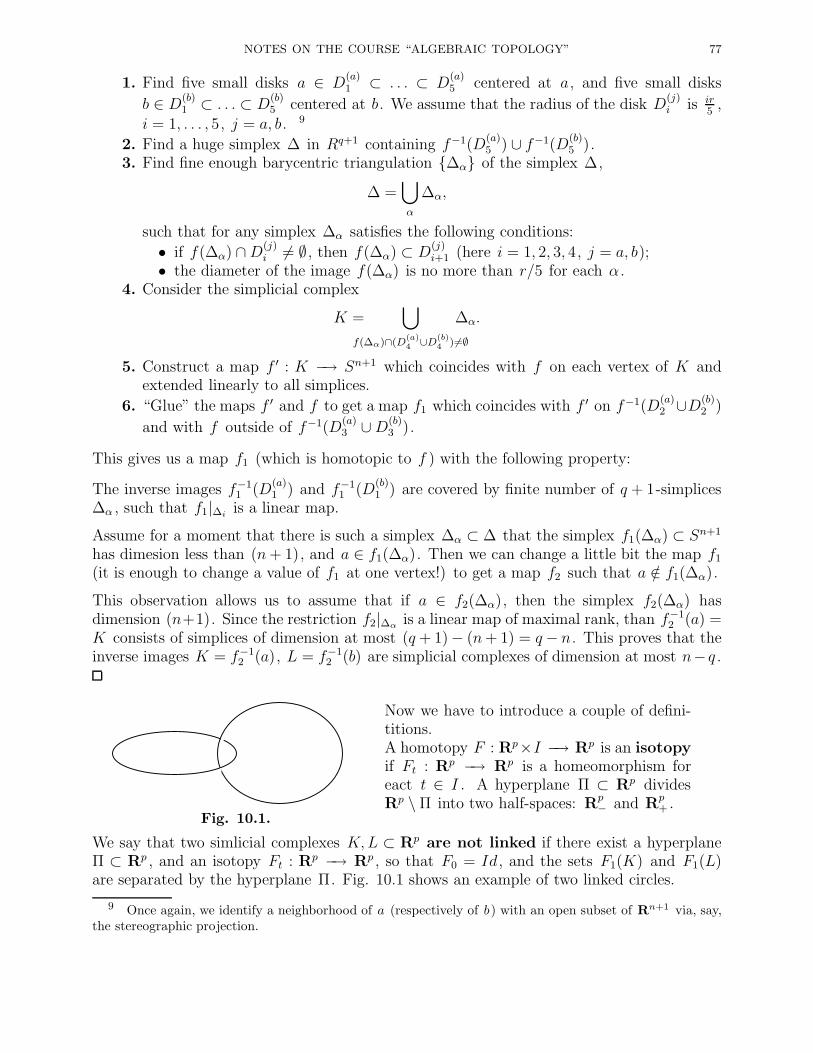
NOTES ON THE COURSE “ALGEBRAIC TOPOLOGY” 77
1. Find five small disks a ∈ D(a)1 ⊂ . . . ⊂ D
(a)5 centered at a, and five small disks
b ∈ D(b)1 ⊂ . . . ⊂ D
(b)5 centered at b. We assume that the radius of the disk D
(j)i is ir
5,
i = 1, . . . , 5, j = a, b. 9
2. Find a huge simplex ∆ in Rq+1 containing f−1(D(a)5 ) ∪ f−1(D
(b)5 ).
3. Find fine enough barycentric triangulation ∆α of the simplex ∆,
∆ =⋃
α
∆α,
such that for any simplex ∆α satisfies the following conditions:
• if f(∆α) ∩D(j)i 6= ∅ , then f(∆α) ⊂ D
(j)i+1 (here i = 1, 2, 3, 4, j = a, b);
• the diameter of the image f(∆α) is no more than r/5 for each α .4. Consider the simplicial complex
K =⋃
f(∆α)∩(D(a)4 ∪D(b)
4 )6=∅
∆α.
5. Construct a map f ′ : K −→ Sn+1 which coincides with f on each vertex of K andextended linearly to all simplices.
6. “Glue” the maps f ′ and f to get a map f1 which coincides with f ′ on f−1(D(a)2 ∪D(b)
2 )
and with f outside of f−1(D(a)3 ∪D(b)
3 ).
This gives us a map f1 (which is homotopic to f ) with the following property:
The inverse images f−11 (D
(a)1 ) and f−1
1 (D(b)1 ) are covered by finite number of q + 1-simplices
∆α , such that f1|∆iis a linear map.
Assume for a moment that there is such a simplex ∆α ⊂ ∆ that the simplex f1(∆α) ⊂ Sn+1
has dimesion less than (n+ 1), and a ∈ f1(∆α). Then we can change a little bit the map f1
(it is enough to change a value of f1 at one vertex!) to get a map f2 such that a /∈ f1(∆α).
This observation allows us to assume that if a ∈ f2(∆α), then the simplex f2(∆α) hasdimension (n+1). Since the restriction f2|∆α
is a linear map of maximal rank, than f−12 (a) =
K consists of simplices of dimension at most (q + 1)− (n+ 1) = q− n. This proves that theinverse images K = f−1
2 (a), L = f−12 (b) are simplicial complexes of dimension at most n− q .
Fig. 10.1.
Now we have to introduce a couple of defini-titions.A homotopy F : Rp×I −→ Rp is an isotopyif Ft : Rp −→ Rp is a homeomorphism foreact t ∈ I . A hyperplane Π ⊂ Rp dividesRp \ Π into two half-spaces: Rp
− and Rp+ .
We say that two simlicial complexes K,L ⊂ Rp are not linked if there exist a hyperplaneΠ ⊂ Rp , and an isotopy Ft : Rp −→ Rp , so that F0 = Id , and the sets F1(K) and F1(L)are separated by the hyperplane Π. Fig. 10.1 shows an example of two linked circles.
9 Once again, we identify a neighborhood of a (respectively of b) with an open subset of Rn+1 via, say,the stereographic projection.
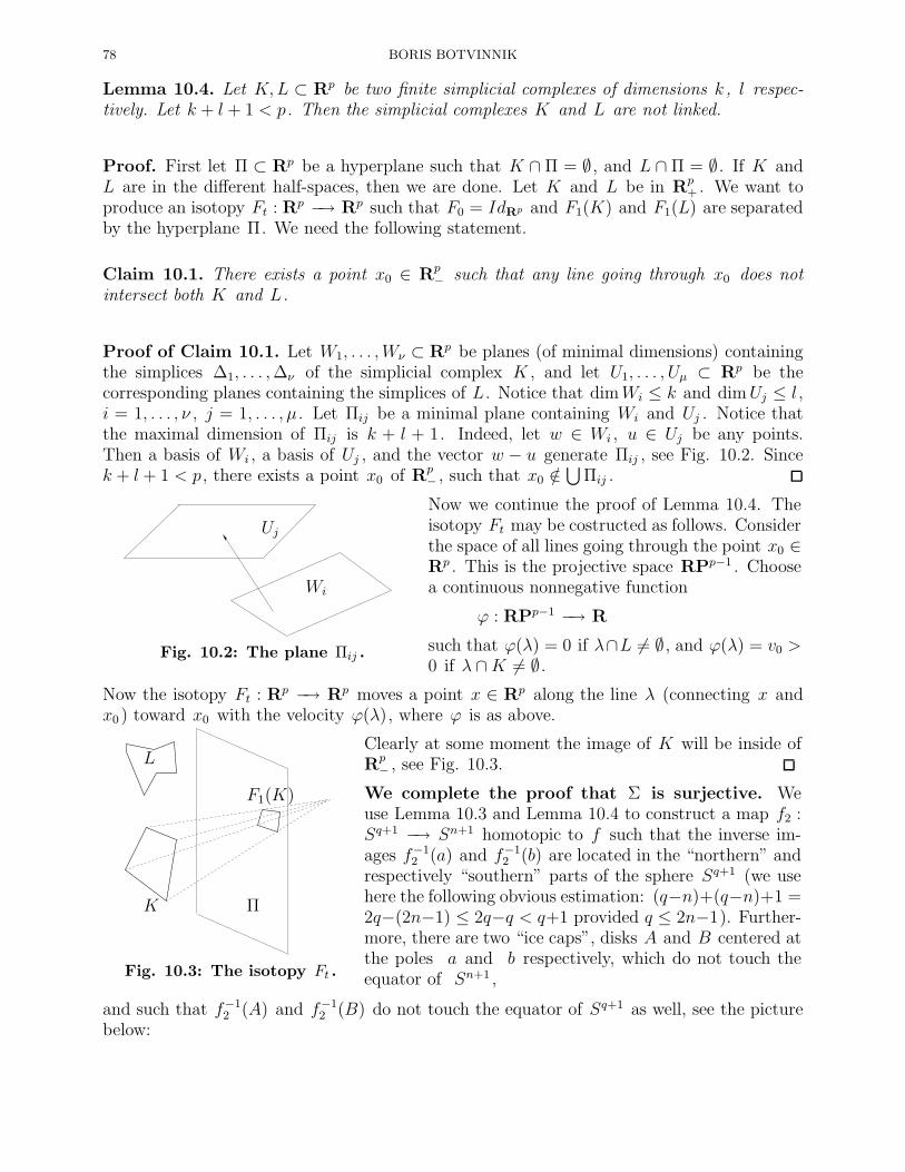
78 BORIS BOTVINNIK
Lemma 10.4. Let K,L ⊂ Rp be two finite simplicial complexes of dimensions k , l respec-tively. Let k + l + 1 < p. Then the simplicial complexes K and L are not linked.
Proof. First let Π ⊂ Rp be a hyperplane such that K ∩ Π = ∅ , and L ∩ Π = ∅ . If K andL are in the different half-spaces, then we are done. Let K and L be in Rp
+ . We want toproduce an isotopy Ft : Rp −→ Rp such that F0 = IdRp and F1(K) and F1(L) are separatedby the hyperplane Π. We need the following statement.
Claim 10.1. There exists a point x0 ∈ Rp− such that any line going through x0 does not
intersect both K and L.
Proof of Claim 10.1. Let W1, . . . ,Wν ⊂ Rp be planes (of minimal dimensions) containingthe simplices ∆1, . . . ,∆ν of the simplicial complex K , and let U1, . . . , Uµ ⊂ Rp be thecorresponding planes containing the simplices of L. Notice that dimWi ≤ k and dimUj ≤ l ,i = 1, . . . , ν , j = 1, . . . , µ . Let Πij be a minimal plane containing Wi and Uj . Notice thatthe maximal dimension of Πij is k + l + 1. Indeed, let w ∈ Wi , u ∈ Uj be any points.Then a basis of Wi , a basis of Uj , and the vector w − u generate Πij , see Fig. 10.2. Sincek + l + 1 < p, there exists a point x0 of Rp
− , such that x0 /∈⋃
Πij .
Wi
Uj
Fig. 10.2: The plane Πij .
Now we continue the proof of Lemma 10.4. Theisotopy Ft may be costructed as follows. Considerthe space of all lines going through the point x0 ∈Rp . This is the projective space RPp−1 . Choosea continuous nonnegative function
ϕ : RPp−1 −→ R
such that ϕ(λ) = 0 if λ∩L 6= ∅ , and ϕ(λ) = v0 >0 if λ ∩K 6= ∅ .
Now the isotopy Ft : Rp −→ Rp moves a point x ∈ Rp along the line λ (connecting x andx0 ) toward x0 with the velocity ϕ(λ), where ϕ is as above.
K
L
F1(K)
Π
Fig. 10.3: The isotopy Ft .
Clearly at some moment the image of K will be inside ofRp
− , see Fig. 10.3.
We complete the proof that Σ is surjective. Weuse Lemma 10.3 and Lemma 10.4 to construct a map f2 :Sq+1 −→ Sn+1 homotopic to f such that the inverse im-ages f−1
2 (a) and f−12 (b) are located in the “northern” and
respectively “southern” parts of the sphere Sq+1 (we usehere the following obvious estimation: (q−n)+(q−n)+1 =2q−(2n−1) ≤ 2q−q < q+1 provided q ≤ 2n−1). Further-more, there are two “ice caps”, disks A and B centered atthe poles a and b respectively, which do not touch theequator of Sn+1 ,
and such that f−12 (A) and f−1
2 (B) do not touch the equator of Sq+1 as well, see the picturebelow:
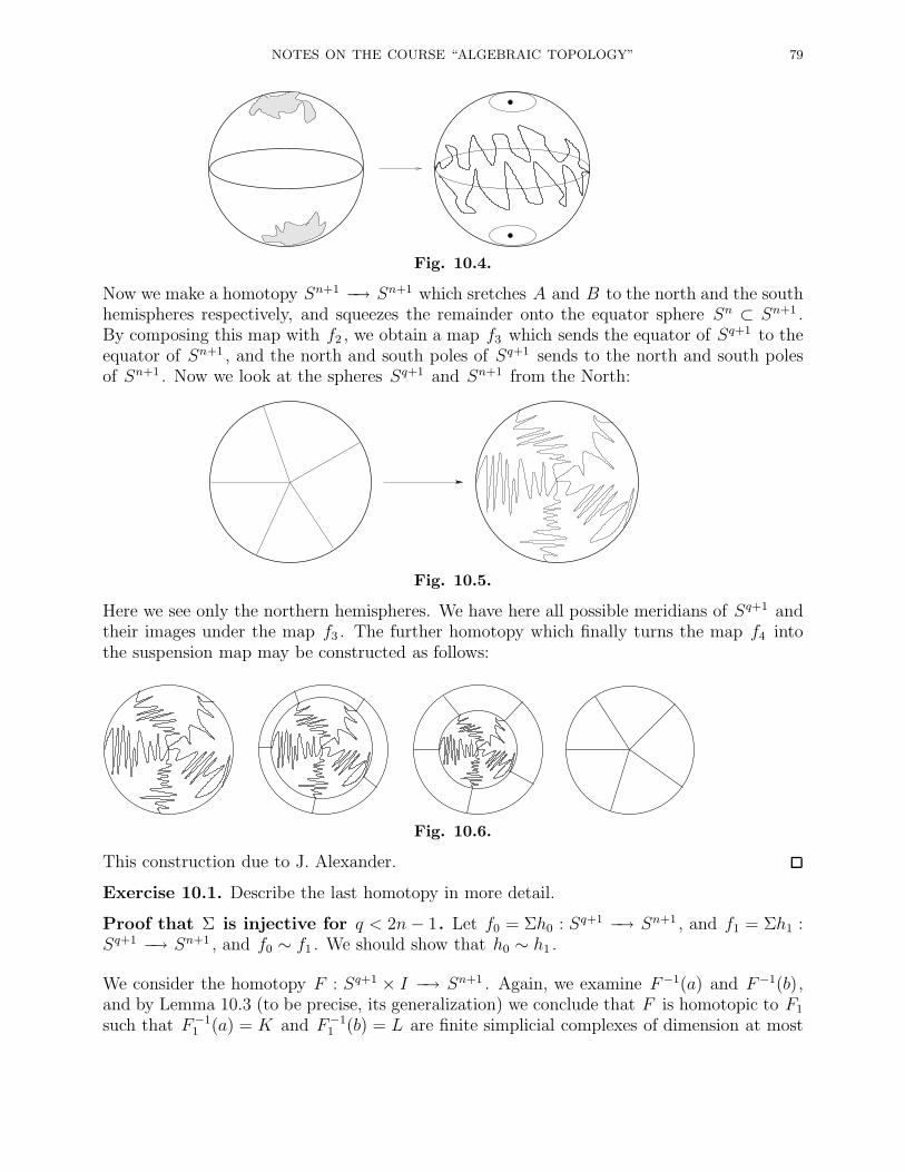
NOTES ON THE COURSE “ALGEBRAIC TOPOLOGY” 79
Fig. 10.4.
Now we make a homotopy Sn+1 −→ Sn+1 which sretches A and B to the north and the southhemispheres respectively, and squeezes the remainder onto the equator sphere Sn ⊂ Sn+1 .By composing this map with f2 , we obtain a map f3 which sends the equator of Sq+1 to theequator of Sn+1 , and the north and south poles of Sq+1 sends to the north and south polesof Sn+1 . Now we look at the spheres Sq+1 and Sn+1 from the North:
Fig. 10.5.
Here we see only the northern hemispheres. We have here all possible meridians of Sq+1 andtheir images under the map f3 . The further homotopy which finally turns the map f4 intothe suspension map may be constructed as follows:
Fig. 10.6.
This construction due to J. Alexander.
Exercise 10.1. Describe the last homotopy in more detail.
Proof that Σ is injective for q < 2n− 1. Let f0 = Σh0 : Sq+1 −→ Sn+1 , and f1 = Σh1 :Sq+1 −→ Sn+1 , and f0 ∼ f1 . We should show that h0 ∼ h1 .
We consider the homotopy F : Sq+1 × I −→ Sn+1 . Again, we examine F−1(a) and F−1(b),and by Lemma 10.3 (to be precise, its generalization) we conclude that F is homotopic to F1
such that F−11 (a) = K and F−1
1 (b) = L are finite simplicial complexes of dimension at most
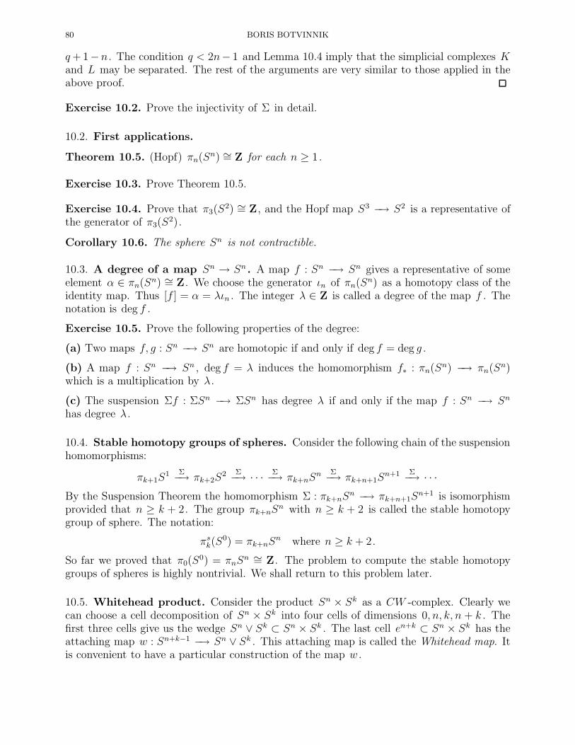
80 BORIS BOTVINNIK
q+ 1−n. The condition q < 2n− 1 and Lemma 10.4 imply that the simplicial complexes Kand L may be separated. The rest of the arguments are very similar to those applied in theabove proof.
Exercise 10.2. Prove the injectivity of Σ in detail.
10.2. First applications.
Theorem 10.5. (Hopf) πn(Sn) ∼= Z for each n ≥ 1.
Exercise 10.3. Prove Theorem 10.5.
Exercise 10.4. Prove that π3(S2) ∼= Z, and the Hopf map S3 −→ S2 is a representative of
the generator of π3(S2).
Corollary 10.6. The sphere Sn is not contractible.
10.3. A degree of a map Sn → Sn . A map f : Sn −→ Sn gives a representative of someelement α ∈ πn(Sn) ∼= Z. We choose the generator ιn of πn(S
n) as a homotopy class of theidentity map. Thus [f ] = α = λιn . The integer λ ∈ Z is called a degree of the map f . Thenotation is deg f .
Exercise 10.5. Prove the following properties of the degree:
(a) Two maps f, g : Sn −→ Sn are homotopic if and only if deg f = deg g .
(b) A map f : Sn −→ Sn , deg f = λ induces the homomorphism f∗ : πn(Sn) −→ πn(S
n)which is a multiplication by λ.
(c) The suspension Σf : ΣSn −→ ΣSn has degree λ if and only if the map f : Sn −→ Sn
has degree λ.
10.4. Stable homotopy groups of spheres. Consider the following chain of the suspensionhomomorphisms:
πk+1S1 Σ−→ πk+2S
2 Σ−→ · · · Σ−→ πk+nSn Σ−→ πk+n+1S
n+1 Σ−→ · · ·By the Suspension Theorem the homomorphism Σ : πk+nS
n −→ πk+n+1Sn+1 is isomorphism
provided that n ≥ k + 2. The group πk+nSn with n ≥ k + 2 is called the stable homotopy
group of sphere. The notation:
πsk(S0) = πk+nS
n where n ≥ k + 2 .
So far we proved that π0(S0) = πnS
n ∼= Z. The problem to compute the stable homotopygroups of spheres is highly nontrivial. We shall return to this problem later.
10.5. Whitehead product. Consider the product Sn × Sk as a CW -complex. Clearly wecan choose a cell decomposition of Sn × Sk into four cells of dimensions 0, n, k, n + k . Thefirst three cells give us the wedge Sn ∨ Sk ⊂ Sn × Sk . The last cell en+k ⊂ Sn × Sk has theattaching map w : Sn+k−1 −→ Sn ∨ Sk . This attaching map is called the Whitehead map. Itis convenient to have a particular construction of the map w .
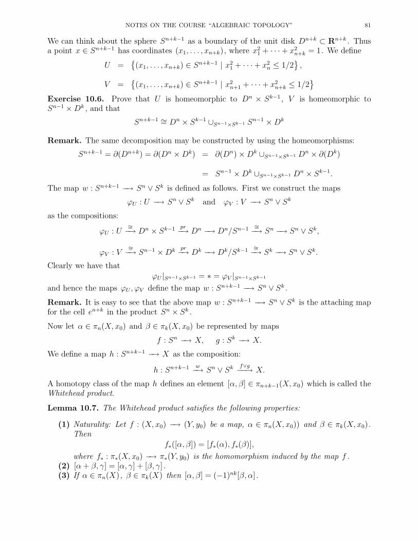
NOTES ON THE COURSE “ALGEBRAIC TOPOLOGY” 81
We can think about the sphere Sn+k−1 as a boundary of the unit disk Dn+k ⊂ Rn+k . Thusa point x ∈ Sn+k−1 has coordinates (x1, . . . , xn+k), where x2
1 + · · ·+ x2n+k = 1. We define
U =(x1, . . . , xn+k) ∈ Sn+k−1 | x2
1 + · · ·+ x2n ≤ 1/2
,
V =(x1, . . . , xn+k) ∈ Sn+k−1 | x2
n+1 + · · ·+ x2n+k ≤ 1/2
Exercise 10.6. Prove that U is homeomorphic to Dn × Sk−1 , V is homeomorphic toSn−1 ×Dk , and that
Sn+k−1 ∼= Dn × Sk−1 ∪Sn−1×Sk−1 Sn−1 ×Dk
Remark. The same decomposition may be constructed by using the homeomorphisms:
Sn+k−1 = ∂(Dn+k) = ∂(Dn ×Dk) = ∂(Dn)×Dk ∪Sn−1×Sk−1 Dn × ∂(Dk)
= Sn−1 ×Dk ∪Sn−1×Sk−1 Dn × Sk−1.
The map w : Sn+k−1 −→ Sn ∨ Sk is defined as follows. First we construct the maps
ϕU : U −→ Sn ∨ Sk and ϕV : V −→ Sn ∨ Sk
as the compositions:
ϕU : U∼=−→ Dn × Sk−1 pr−→ Dn −→ Dn/Sn−1
∼=−→ Sn −→ Sn ∨ Sk,
ϕV : V∼=−→ Sn−1 ×Dk pr−→ Dk −→ Dk/Sk−1
∼=−→ Sk −→ Sn ∨ Sk.Clearly we have that
ϕU |Sn−1×Sk−1 = ∗ = ϕV |Sn−1×Sk−1
and hence the maps ϕU , ϕV define the map w : Sn+k−1 −→ Sn ∨ Sk .Remark. It is easy to see that the above map w : Sn+k−1 −→ Sn ∨ Sk is the attaching mapfor the cell en+k in the product Sn × Sk .Now let α ∈ πn(X, x0) and β ∈ πk(X, x0) be represented by maps
f : Sn −→ X, g : Sk −→ X.
We define a map h : Sn+k−1 −→ X as the composition:
h : Sn+k−1 w−→ Sn ∨ Sk f∨g−−→ X.
A homotopy class of the map h defines an element [α, β] ∈ πn+k−1(X, x0) which is called theWhitehead product.
Lemma 10.7. The Whitehead product satisfies the following properties:
(1) Naturality: Let f : (X, x0) −→ (Y, y0) be a map, α ∈ πn(X, x0)) and β ∈ πk(X, x0).Then
f∗([α, β]) = [f∗(α), f∗(β)],
where f∗ : π∗(X, x0) −→ π∗(Y, y0) is the homomorphism induced by the map f .(2) [α + β, γ] = [α, γ] + [β, γ].(3) If α ∈ πn(X), β ∈ πk(X) then [α, β] = (−1)nk[β, α].
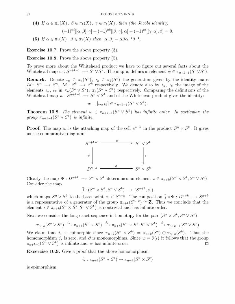
82 BORIS BOTVINNIK
(4) If α ∈ πn(X), β ∈ πk(X), γ ∈ πℓ(X), then (the Jacobi identity)
(−1)nℓ[[α, β], γ] + (−1)nk[[β, γ], α] + (−1)kℓ[[γ, α], β] = 0.
(5) If α ∈ π1(X), β ∈ π1(X) then [α, β] = αβα−1β−1 .
Exercise 10.7. Prove the above property (3).
Exercise 10.8. Prove the above property (5).
To prove more about the Whitehead product we have to figure out several facts about theWhitehead map w : Sn+k−1 −→ Sn∨Sk . The map w defines an element w ∈ πn+k−1(S
n∨Sk).Remark. Denote ιn ∈ πn(S
n), ιk ∈ πk(Sk) the generators given by the identity maps
Id : Sn −→ Sn , Id : Sk −→ Sk respectively. We denote also by ιn , ιk the image of theelements ιn , ιk in πn(S
n ∨ Sk), πk(Sn ∨ Sk) respectively. Comparing the definitions of theWhitehead map w : Sn+k−1 −→ Sn ∨ Sk and of the Whitehead product gives the identity:
w = [ιn, ιk] ∈ πn+k−1(Sn ∨ Sk).
Theorem 10.8. The element w ∈ πn+k−1(Sn ∨ Sk) has infinite order. In particular, the
group πn+k−1(Sn ∨ Sk) is infinite.
Proof. The map w is the attaching map of the cell en+k in the product Sn × Sk . It givesus the commutative diagram:
Sn+k−1
?
p′
Sn ∨ Sk
?
i
-w
Dn+k Sn × Sk-Φ
Clearly the map Φ : Dn+k −→ Sn × Sk determines an element ι ∈ πn+k(Sn × Sk, Sn ∨ Sk).
Consider the map
j : (Sn × Sk, Sn ∨ Sk) −→ (Sn+k, s0)
which maps Sn ∨ Sk to the base point s0 ∈ Sn+k . The composition j Φ : Dn+k −→ Sn+k
is a representative of a generator of the group πn+k(Sn+k) ∼= Z. Thus we conclude that the
element ι ∈ πn+k(Sn × Sk, Sn ∨ Sk) is nontrivial and has infinite order.
Next we consider the long exact sequence in homotopy for the pair (Sn × Sk, Sn ∨ Sk):
πn+k(Sn ∨ Sk) i∗−→ πn+k(S
n × Sk) j∗−→ πn+k(Sn × Sk, Sn ∨ Sk) ∂−→ πn+k−1(S
n ∨ Sk)We claim that i∗ is epimorphic since πn+k(S
n × Sk) = πn+k(Sn) ⊕ πn+k(S
k). Thus thehomomorphism j∗ is zero, and ∂ is monomorphims. Since w = ∂(ι) it follows that the groupπn+k−1(S
n ∨ Sk) is infinite and w has infinite order.
Excercise 10.9. Give a proof that the above homomorphism
i∗ : πn+k(Sn ∨ Sk)→ πn+k(S
n × Sk)is epimorphism.
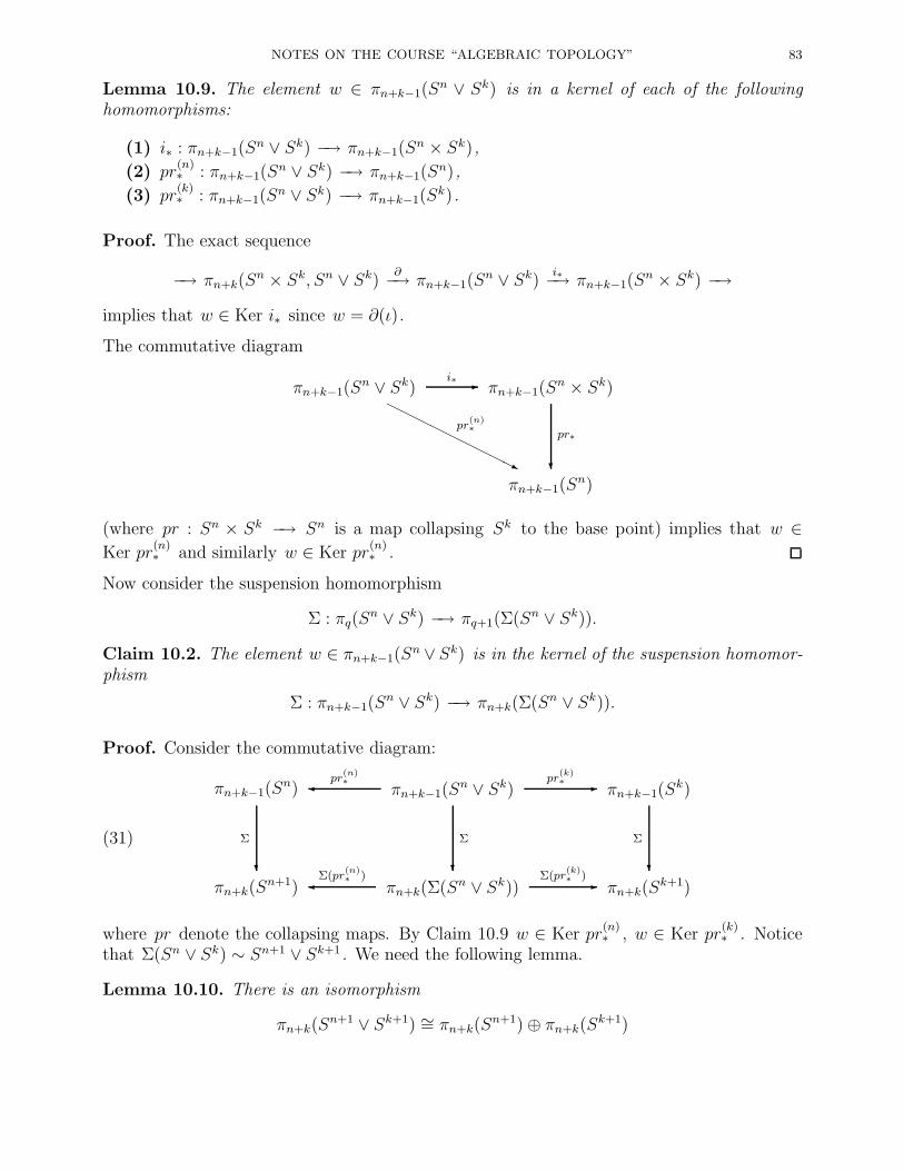
NOTES ON THE COURSE “ALGEBRAIC TOPOLOGY” 83
Lemma 10.9. The element w ∈ πn+k−1(Sn ∨ Sk) is in a kernel of each of the following
homomorphisms:
(1) i∗ : πn+k−1(Sn ∨ Sk) −→ πn+k−1(S
n × Sk),(2) pr
(n)∗ : πn+k−1(S
n ∨ Sk) −→ πn+k−1(Sn),
(3) pr(k)∗ : πn+k−1(S
n ∨ Sk) −→ πn+k−1(Sk).
Proof. The exact sequence
−→ πn+k(Sn × Sk, Sn ∨ Sk) ∂−→ πn+k−1(S
n ∨ Sk) i∗−→ πn+k−1(Sn × Sk) −→
implies that w ∈ Ker i∗ since w = ∂(ι).
The commutative diagram
πn+k−1(Sn ∨ Sk)
HHHHHHHHHj
pr(n)∗
πn+k−1(Sn × Sk)
?
pr∗
-i∗
πn+k−1(Sn)
(where pr : Sn × Sk −→ Sn is a map collapsing Sk to the base point) implies that w ∈Ker pr
(n)∗ and similarly w ∈ Ker pr
(n)∗ .
Now consider the suspension homomorphism
Σ : πq(Sn ∨ Sk) −→ πq+1(Σ(Sn ∨ Sk)).
Claim 10.2. The element w ∈ πn+k−1(Sn ∨ Sk) is in the kernel of the suspension homomor-
phism
Σ : πn+k−1(Sn ∨ Sk) −→ πn+k(Σ(Sn ∨ Sk)).
Proof. Consider the commutative diagram:
(31)
πn+k−1(Sn)
?
Σ
πn+k−1(Sn ∨ Sk)
?
Σ
πn+k−1(Sk)
?
Σ
pr(n)∗ -pr
(k)∗
πn+k(Sn+1) πn+k(Σ(Sn ∨ Sk)) πn+k(S
k+1)Σ(pr(n)∗ ) -Σ(pr
(k)∗ )
where pr denote the collapsing maps. By Claim 10.9 w ∈ Ker pr(n)∗ , w ∈ Ker pr
(k)∗ . Notice
that Σ(Sn ∨ Sk) ∼ Sn+1 ∨ Sk+1 . We need the following lemma.
Lemma 10.10. There is an isomorphism
πn+k(Sn+1 ∨ Sk+1) ∼= πn+k(S
n+1)⊕ πn+k(Sk+1)
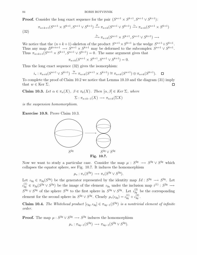
84 BORIS BOTVINNIK
Proof. Consider the long exact sequence for the pair (Sn+1 × Sk+1, Sn+1 ∨ Sk+1):
(32)πn+k+1(S
n+1 × Sk+1, Sn+1 ∨ Sk+1)∂−→ πn+k(S
n+1 ∨ Sk+1)i∗−→ πn+k(S
n+1 × Sk+1)
j∗−→ πn+k(Sn+1 × Sk+1, Sn+1 ∨ Sk+1) −→
We notice that the (n+k+1)-skeleton of the product Sn+1×Sk+1 is the wedge Sn+1∨Sk+1 .Thus any map Dk+n+1 −→ Sn+1 × Sk+1 may be deformed to the subcomplex Sn+1 ∨ Sk+1 .Thus πn+k+1(S
n+1 × Sk+1, Sn+1 ∨ Sk+1) = 0. The same argument gives that
πn+k(Sn+1 × Sk+1, Sn+1 ∨ Sk+1) = 0.
Thus the long exact sequence (32) gives the isomorphism:
i∗ : πn+k(Sn+1 ∨ Sk+1)
∼=−→ πn+k(Sn+1 × Sk+1) ∼= πn+k(S
n+1)⊕ πn+k(Sk+1).
To complete the proof of Claim 10.2 we notice that Lemma 10.10 and the diagram (31) implythat w ∈ Ker Σ.
Claim 10.3. Let α ∈ πn(X), β ∈ πk(X). Then [α, β] ∈ Ker Σ, where
Σ : πn+k−1(X) −→ πn+k(ΣX)
is the suspension homomorphism.
Exercise 10.9. Prove Claim 10.3.
S2q S2q ∨ S2q
Fig. 10.7.
Now we want to study a particular case. Consider the map µ : S2q −→ S2q ∨ S2q whichcollapses the equator sphere, see Fig. 10.7. It induces the homomorphism
µ∗ : π∗(S2q) −→ π∗(S
2q ∨ S2q).
Let ι2q ∈ π2q(S2q) be the generator represented by the identity map Id : S2q −→ S2q . Let
ι(1)2q ∈ π2q(S
2q ∨ S2q) be the image of the element ι2q under the inclusion map i(1) : S2q −→S2q ∨ S2q of the sphere S2q to the first sphere in S2q ∨ S2q . Let ι
(2)2q be the corresponding
element for the second sphere in S2q ∨ S2q . Clearly µ∗(ι2q) = ι(1)2q + ι
(2)2q .
Claim 10.4. The Whitehead product [ι2q, ι2q] ∈ π4q−1(S2q) is a nontrivial element of infinite
order.
Proof. The map µ : S2q ∨ S2q −→ S2q induces the homomorphism
µ∗ : π4q−1(S2q) −→ π4q−1(S
2q ∨ S2q).
NOTES ON THE COURSE “ALGEBRAIC TOPOLOGY” 85
By naturality we have that
µ∗([ι2q, ι2q]) = [µ∗(ι2q), µ∗(ι2q)] = [ι(1)2q + ι
(2)2q , ι
(1)2q + ι
(2)2q ].
By additivity and commutativity (Claim 10.7 (2), (3)) we also have:
µ∗([ι2q, ι2q]) = [ι(1)2q + ι
(2)2q , ι
(1)2q + ι
(2)2q ]
= [ι(1)2q , ι
(1)2q ] + [ι
(1)2q , ι
(2)2q ] + [ι
(2)2q , ι
(1)2q ] + [ι
(2)2q , ι
(2)2q ]
= [ι(1)2q , ι
(1)2q ] + [ι
(1)2q , ι
(2)2q ] + (−1)4q[ι
(1)2q , ι
(2)2q ] + [ι
(2)2q , ι
(2)2q ]
= [ι(1)2q , ι
(1)2q ] + [ι
(2)2q , ι
(2)2q ] + 2w2q
where w2q = [ι(1)2q , ι
(2)2q ]. Notice that we used the fact that the sphere S2q is even-dimensional.
Now assume that the element [ι2q, ι2q] ∈ π4q−1(S2q) has finite order. Then the elements
[ι(j)2q , ι
(j)2q ] ∈ π4q−1(S
2q), j = 1, 2 also have finite order since ι(j)2q is the image of the generator
ι2q under the homomorphism π2q(S2q) −→ π2q(S
2q ∨ S2q). Then it follows that for someinteger λ
0 = µ∗(λ[ι2q, ι2q]) = λ[ι(1)2q , ι
(1)2q ] + λ[ι
(2)2q , ι
(2)2q ] + 2λw2q = 2λw2q.
This contradicts to Claim 10.8. Thus the element [ι2q, ι2q] ∈ π4q−1(S2q) has infinite order.
We specify Claims 10.3, 10.4 to get so called “hard part” of the Suspension Theorem.
Theorem 10.11. (1) The Whitehead product [ι2q, ι2q] ∈ π4q−1(S2q) has infinite order.
(2) The Whitehead product [ι2q, ι2q] ∈ π4q−1(S2q) is in the kernel of the suspension homo-
morphism, i.e. Σ([ι2q , ι2q]) = 0 in π4q(S2q+1).
Remark. Actually, π4q−1(S2q) ∼= Z⊕finite group and these groups are the only homotopy
groups of spheres (besides πn(Sn)) which are infinite. We shall return to the Whitehead
product to study the Hopf invariant.
Now we consider the product Sn × Sk .Corollary 10.12. The suspension Σ(Sn × Sk) is homotopy equivalent to the wedge
Sn+1 ∨ Sk+1 ∨ Sn+k+1.
Exercise 10.10. Prove Corollary 10.12.
86 BORIS BOTVINNIK
11. Homotopy groups of CW -complexes
11.1. Changing homotopy groups by attaching a cell. Let X be a CW -complex, andf : Sn −→ X be an attaching map for new cell. Let Y = X ∪f Dn+1 . We would like tounderstand how do the homotopy groups π∗X and π∗Y relate to each other.
Theorem 11.1. Let X be a path-connected space (not necessarily a CW -complex) with abase point x0 ∈ X , f : Sn −→ X be a map such that f(s0) = x0 , where s0 is a base point ofSn . Let Y = X ∪fDn+1 , and i : X −→ Y be the inclusion. Then the induced homomorphism
(33) i∗ : πq(X, x0) −→ πq(Y, x0)
(1) is an isomorphism if q < n,(2) is an epimorphism if q = n, and(3) the kernel Ker i∗ : πn(X, x0) −→ πn(Y, x0) is generated by γ−1[f ]γ ∈ πn(X, x0) where
γ ∈ π1(X, x0).
Proof. First we prove a technical result. Let Em be either Dm or Sm . In both cases wechoose Rm to be a subspace of Em :
Sm = Rm ∪ x0 ,
Dm =o
Dm ∪ Sm−1,o
Dm ∼= Rm.
Lemma 11.2. Let h : Em −→ Y be a map, such that h|Em\Rm sends Em \Rm to X . Thenthere exists a map h1 : Em −→ Y homotopic to h such that:
(a) h1|h−1(X) = h|h−1(X) .(b) If m ≤ n then h1(E
m) ⊂ X .(c) If m = n + 1 there exist disks d1, . . . , dr ⊂ Em such that
(c1) h1(Em \
r⋃
s=1
ds) ⊂ X ;
(c2) the restriction h1|ods
:o
ds −→ Dm is a linear homeomorphism, s = 1, . . . , r .
Proof. The proof goes down the line of arguments which we used several times starting withFree Point Lemma. We give here the outline only.
(1) Consider the disks (centered at the same point) Dm1 ⊂ Dm
2 ⊂ Dm3 ⊂ Dm
4 ⊂ Dm5 ⊂ Dm
of radii iρ/5, i = 1, . . . , 5.(2) The set h−1(Dm
5 ) ⊂ Em is compact, furthermore, h−1(Dm5 ) ⊂ Rm ⊂ Em . Choose a
simplex ∆m ⊃ h−1(Dm5 ) and a triangulation ∆α of ∆ such that if h(∆α)∩Dm
i 6= ∅then h(∆α) ⊂ Dm
i+1 for i = 1, 2, 3, 4, and diam(h(∆α)) < ρ/5.
(3) Let K =⋃
h(∆α)∩Dm4 6=∅∆α . Then we construct a map h′ : K −→ Dm by extending linearly
h restricted on the vertices of K .(4) We assume that the center y0 of the disks Dm
i is not in the image of any face of thesimplices ∆α . If it happens to be in such image, we choose a homotopy which moves
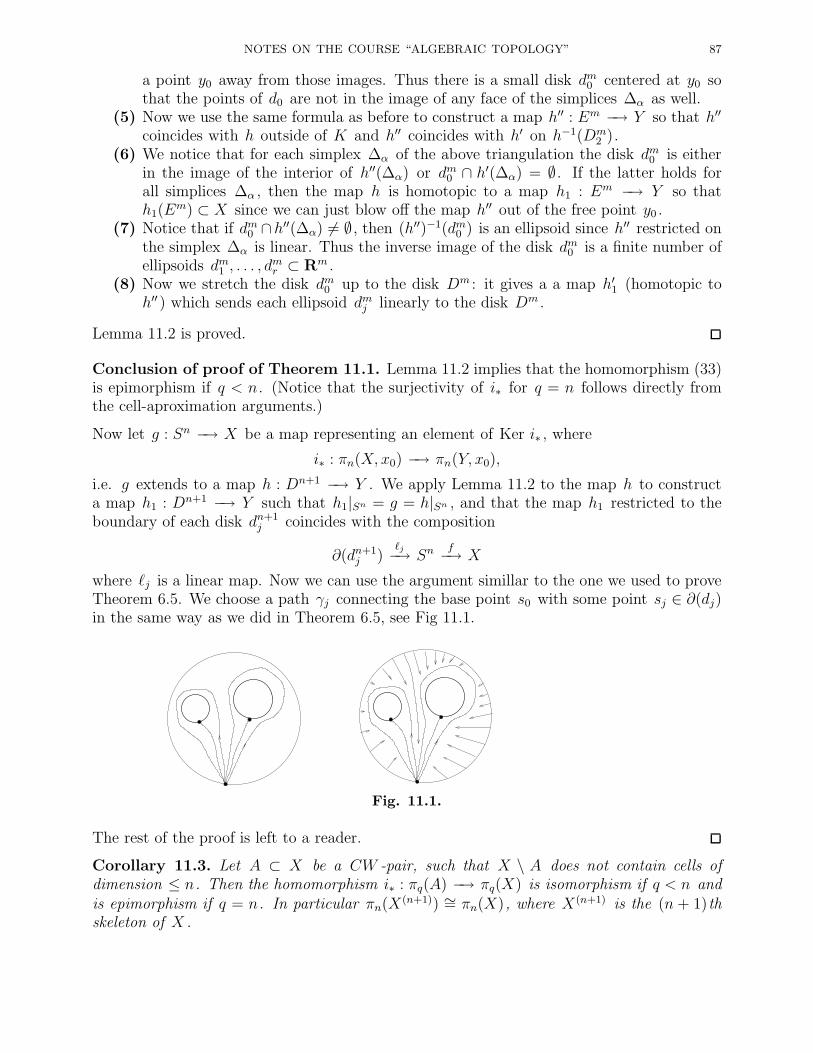
NOTES ON THE COURSE “ALGEBRAIC TOPOLOGY” 87
a point y0 away from those images. Thus there is a small disk dm0 centered at y0 sothat the points of d0 are not in the image of any face of the simplices ∆α as well.
(5) Now we use the same formula as before to construct a map h′′ : Em −→ Y so that h′′
coincides with h outside of K and h′′ coincides with h′ on h−1(Dm2 ).
(6) We notice that for each simplex ∆α of the above triangulation the disk dm0 is eitherin the image of the interior of h′′(∆α) or dm0 ∩ h′(∆α) = ∅ . If the latter holds forall simplices ∆α , then the map h is homotopic to a map h1 : Em −→ Y so thath1(E
m) ⊂ X since we can just blow off the map h′′ out of the free point y0 .(7) Notice that if dm0 ∩h′′(∆α) 6= ∅ , then (h′′)−1(dm0 ) is an ellipsoid since h′′ restricted on
the simplex ∆α is linear. Thus the inverse image of the disk dm0 is a finite number ofellipsoids dm1 , . . . , d
mr ⊂ Rm .
(8) Now we stretch the disk dm0 up to the disk Dm : it gives a a map h′1 (homotopic toh′′ ) which sends each ellipsoid dmj linearly to the disk Dm .
Lemma 11.2 is proved.
Conclusion of proof of Theorem 11.1. Lemma 11.2 implies that the homomorphism (33)is epimorphism if q < n. (Notice that the surjectivity of i∗ for q = n follows directly fromthe cell-aproximation arguments.)
Now let g : Sn −→ X be a map representing an element of Ker i∗ , where
i∗ : πn(X, x0) −→ πn(Y, x0),
i.e. g extends to a map h : Dn+1 −→ Y . We apply Lemma 11.2 to the map h to constructa map h1 : Dn+1 −→ Y such that h1|Sn = g = h|Sn , and that the map h1 restricted to theboundary of each disk dn+1
j coincides with the composition
∂(dn+1j )
ℓj−→ Snf−→ X
where ℓj is a linear map. Now we can use the argument simillar to the one we used to proveTheorem 6.5. We choose a path γj connecting the base point s0 with some point sj ∈ ∂(dj)in the same way as we did in Theorem 6.5, see Fig 11.1.
Fig. 11.1.
The rest of the proof is left to a reader.
Corollary 11.3. Let A ⊂ X be a CW -pair, such that X \ A does not contain cells ofdimension ≤ n. Then the homomorphism i∗ : πq(A) −→ πq(X) is isomorphism if q < n andis epimorphism if q = n. In particular πn(X
(n+1)) ∼= πn(X), where X(n+1) is the (n + 1)thskeleton of X .
88 BORIS BOTVINNIK
11.2. Homotopy groups of a wedge.
Theorem 11.4. Let X be an n-connected CW -complex, and Y be a k -connected CW -complex. Then
(1) πq(X ∨ Y ) ∼= πq(X)⊕ πq(Y ) for q ≤ n+ k ;(2) for each q ≥ 1 the group πq(X∨Y ) contains a direct summand isomorphic to πq(X)⊕
πq(Y ).
Proof. By Theorem 5.11 the CW -complexes X and Y are homotopy equivalent to CW -complexes without cells in dimensions in between 0 and n + 1 (for X ) and in between 0and k + 1 (for Y ). Thus we may assume that X and Y are such complexes. Consider theproduct X×Y with the product cell-structure. The wedge X ∨Y is a subcomplex of X×Y .Furthermore the difference X × Y \ X ∨ Y has cells of dimension at least n + k + 2. ByCorollary 11.3,
πq(X ∨ Y ) ∼= πq(X × Y ) ∼= πq(X)⊕ πq(Y ).
To prove the second statement we notice that the composition
πq(X)⊕ πq(Y )iX∗⊕iY
∗−−−−→ πq(X ∨ Y ) −→ πq(X × Y )∼=−→ πq(X)⊕ πq(Y ),
(where iX : X −→ X ∨ Y , iY : Y −→ X ∨ Y are the caninical embeddings) is the identityhomomorphism.
Corollary 11.5. There is an isomorphism πn(Sn ∨ · · · ∨ Sn) ∼= Z⊕ · · · ⊕ Z with generators
induced by the embeddings Sn −→ Sn ∨ · · · ∨ Sn .
Exercise 11.1. Let X be an n-connected CW -complex, and Y be a k -connected CW -complex. Prove the isomorphism:
πn+k+1(X ∨ Y ) ∼= πn+k+1(X)⊕ πn+k+1(Y )⊕ [πn+1(X), πk+1(Y )].
In particular it follows that π3(S2 ∨ S2) ∼= Z⊕ Z⊕ Z.
11.3. The first nontrivial homotopy group of a CW -complex. Let X be (n − 1)-connected CW -complex. We know very well that the homotopy groups πq(X) = 0 if q ≤n − 1. Our goal is to describe the group πn(X). Again we can assume that X does notcontain cells of dimension in between 0 and n. Then the n-skeleton X(n) is a wedge ofspheres: X(n) = Sn1 ∨ · · · ∨ Sns . Let gi : Sn −→ Sn1 ∨ · · · ∨ Sns be the embedding of the i-thsphere, and let rj : Sn −→ Sn1 ∨· · ·∨Sns be the attaching maps of the n+1 cells en+1
1 , . . . , en+1β .
The maps gi determine the generators of the group πn(X(n)), and let ρj ∈ πn(X(n)) be the
elements determined by the maps rj . The following theorem is a straightforward corollary ofTheorem 11.1.
Theorem 11.6. The homotopy group πn(X) is isomorphic to the factor group of the homo-topy group πn(X
(n)) ∼= Z⊕ · · · ⊕ Z by the subgroup generated by ρj , j = 1, . . . , β .
Remark. Theorem 11.6 is analogous to Theorem 6.5 about the fundamental group. Thisresult gives an impression that we can calculate the first nontrivial homotopy group of anyCW -complex without any problems. However, we do not offer here an efficient algorithm todo this calculation. The difficulty shows up when we start with any CW -complex X and
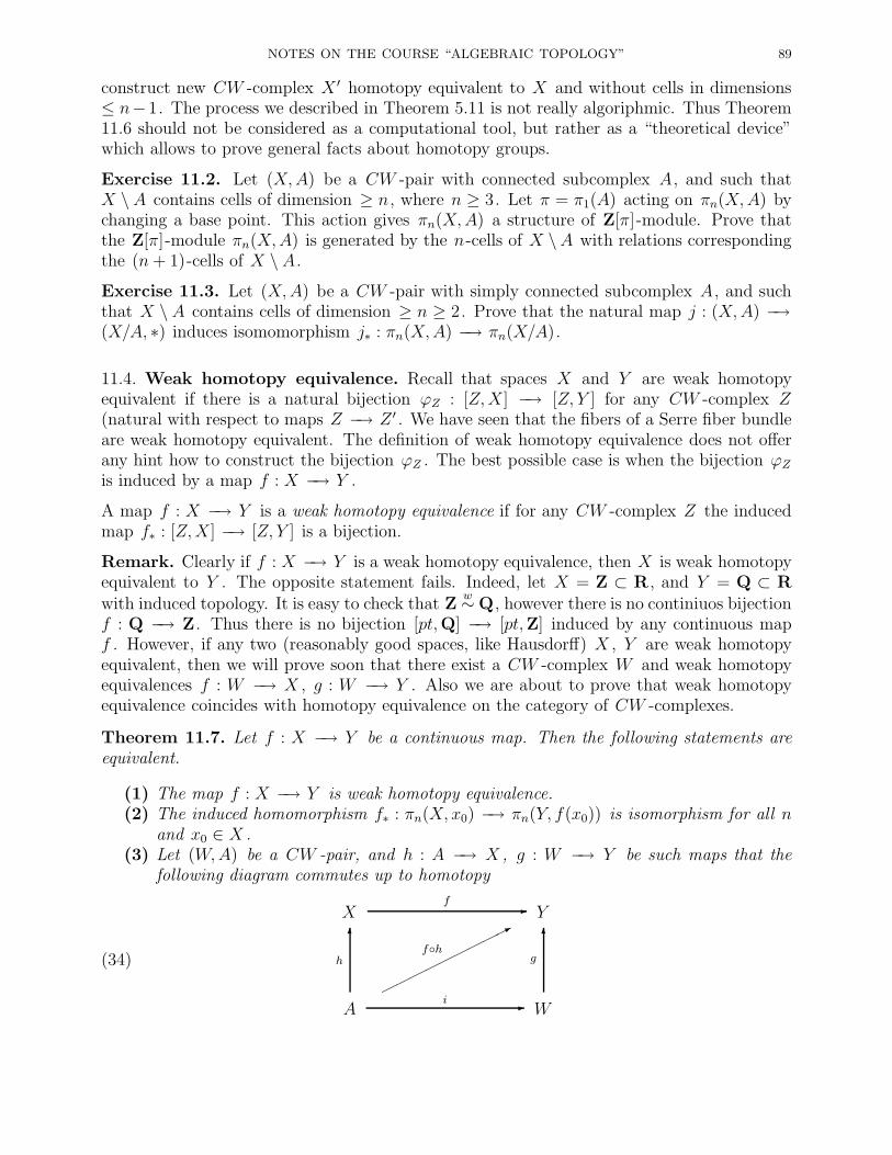
NOTES ON THE COURSE “ALGEBRAIC TOPOLOGY” 89
construct new CW -complex X ′ homotopy equivalent to X and without cells in dimensions≤ n−1. The process we described in Theorem 5.11 is not really algoriphmic. Thus Theorem11.6 should not be considered as a computational tool, but rather as a “theoretical device”which allows to prove general facts about homotopy groups.
Exercise 11.2. Let (X,A) be a CW -pair with connected subcomplex A, and such thatX \ A contains cells of dimension ≥ n, where n ≥ 3. Let π = π1(A) acting on πn(X,A) bychanging a base point. This action gives πn(X,A) a structure of Z[π]-module. Prove thatthe Z[π]-module πn(X,A) is generated by the n-cells of X \A with relations correspondingthe (n+ 1)-cells of X \ A.
Exercise 11.3. Let (X,A) be a CW -pair with simply connected subcomplex A, and suchthat X \ A contains cells of dimension ≥ n ≥ 2. Prove that the natural map j : (X,A) −→(X/A, ∗) induces isomomorphism j∗ : πn(X,A) −→ πn(X/A).
11.4. Weak homotopy equivalence. Recall that spaces X and Y are weak homotopyequivalent if there is a natural bijection ϕZ : [Z,X] −→ [Z, Y ] for any CW -complex Z(natural with respect to maps Z −→ Z ′ . We have seen that the fibers of a Serre fiber bundleare weak homotopy equivalent. The definition of weak homotopy equivalence does not offerany hint how to construct the bijection ϕZ . The best possible case is when the bijection ϕZis induced by a map f : X −→ Y .
A map f : X −→ Y is a weak homotopy equivalence if for any CW -complex Z the inducedmap f∗ : [Z,X] −→ [Z, Y ] is a bijection.
Remark. Clearly if f : X −→ Y is a weak homotopy equivalence, then X is weak homotopyequivalent to Y . The opposite statement fails. Indeed, let X = Z ⊂ R , and Y = Q ⊂ Rwith induced topology. It is easy to check that Z
w∼Q, however there is no continiuos bijectionf : Q −→ Z. Thus there is no bijection [pt,Q] −→ [pt,Z] induced by any continuous mapf . However, if any two (reasonably good spaces, like Hausdorff) X , Y are weak homotopyequivalent, then we will prove soon that there exist a CW -complex W and weak homotopyequivalences f : W −→ X , g : W −→ Y . Also we are about to prove that weak homotopyequivalence coincides with homotopy equivalence on the category of CW -complexes.
Theorem 11.7. Let f : X −→ Y be a continuous map. Then the following statements areequivalent.
(1) The map f : X −→ Y is weak homotopy equivalence.(2) The induced homomorphism f∗ : πn(X, x0) −→ πn(Y, f(x0)) is isomorphism for all n
and x0 ∈ X .(3) Let (W,A) be a CW -pair, and h : A −→ X , g : W −→ Y be such maps that the
following diagram commutes up to homotopy
(34)
X Y-f
A
6
h
*fh
W
6g
-i
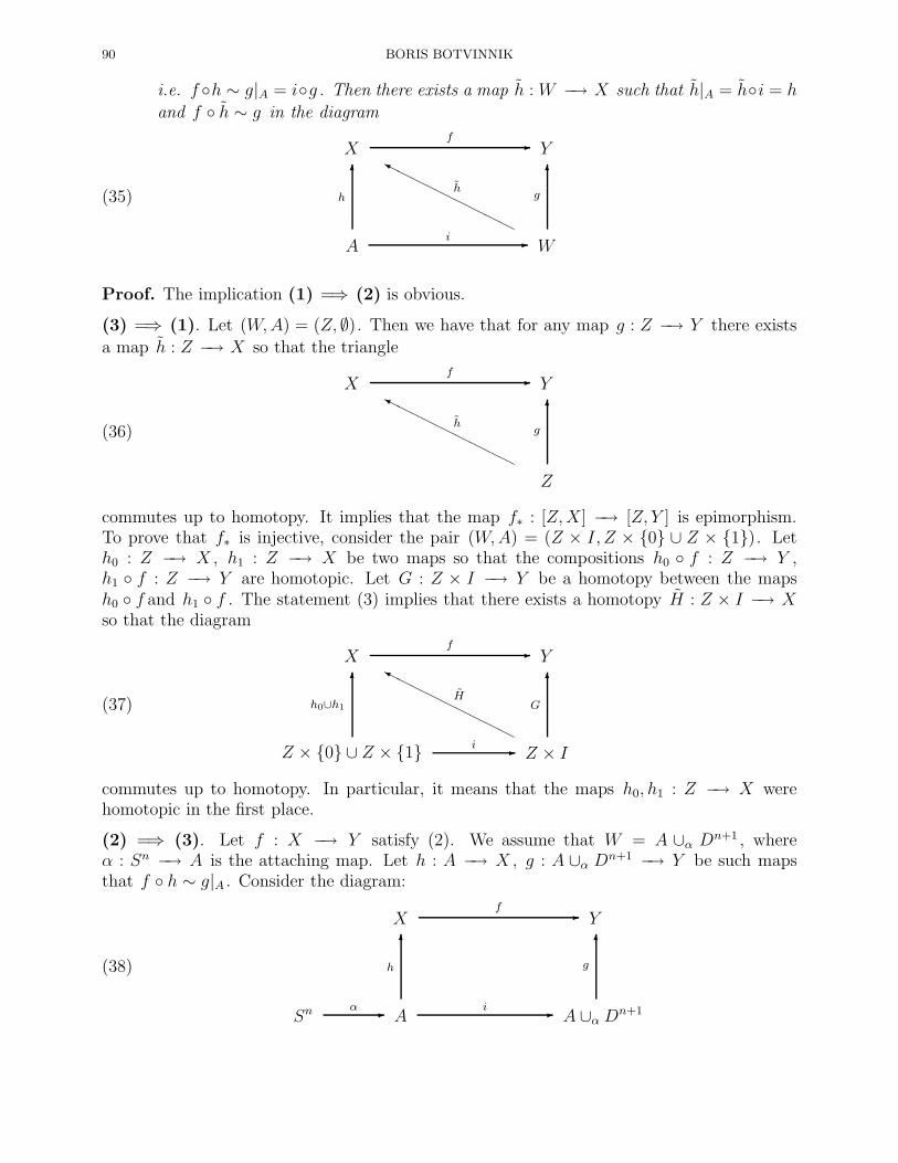
90 BORIS BOTVINNIK
i.e. f h ∼ g|A = ig . Then there exists a map h : W −→ X such that h|A = hi = h
and f h ∼ g in the diagram
(35)
X Y-f
A
6
h
W
6g
HHHHHHHHHYh
-i
Proof. The implication (1) =⇒ (2) is obvious.
(3) =⇒ (1). Let (W,A) = (Z, ∅). Then we have that for any map g : Z −→ Y there exists
a map h : Z −→ X so that the triangle
(36)
X Y-f
Z
6g
HHHHHHHHHYh
commutes up to homotopy. It implies that the map f∗ : [Z,X] −→ [Z, Y ] is epimorphism.To prove that f∗ is injective, consider the pair (W,A) = (Z × I, Z × 0 ∪ Z × 1). Leth0 : Z −→ X , h1 : Z −→ X be two maps so that the compositions h0 f : Z −→ Y ,h1 f : Z −→ Y are homotopic. Let G : Z × I −→ Y be a homotopy between the mapsh0 f and h1 f . The statement (3) implies that there exists a homotopy H : Z × I −→ Xso that the diagram
(37)
X Y-f
Z × 0 ∪ Z × 1
6h0∪h1
Z × I
6
G
HHHHHHHHHYH
-i
commutes up to homotopy. In particular, it means that the maps h0, h1 : Z −→ X werehomotopic in the first place.
(2) =⇒ (3). Let f : X −→ Y satisfy (2). We assume that W = A ∪α Dn+1 , whereα : Sn −→ A is the attaching map. Let h : A −→ X , g : A ∪α Dn+1 −→ Y be such mapsthat f h ∼ g|A . Consider the diagram:
(38)
X Y-f
Sn A
6
h
A ∪α Dn+1
6g
-α -i
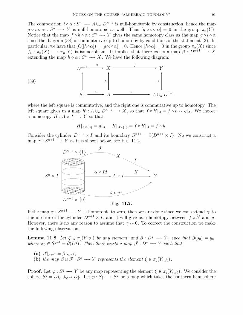
NOTES ON THE COURSE “ALGEBRAIC TOPOLOGY” 91
The composition i α : Sn −→ A∪α Dn+1 is null-homotopic by construction, hence the mapg i α : Sn −→ Y is null-homotopic as well. Thus [g i α] = 0 in the group πn(Y ).Notice that the map f h α : Sn −→ Y gives the same homotopy class as the map g i αsince the diagram (38) is commutative up to homotopy by conditions of the statement (3). Inparticular, we have that f∗([hα]) = [giα] = 0. Hence [hα] = 0 in the group πn(X) sincef∗ : πn(X) −→ πn(Y ) is isomorphism. It implies that there exists a map β : Dn+1 −→ Xextending the map h α : Sn −→ X . We have the following diagram:
(39)
Dn+1 X Y-β -f
Sn
6
A
6
h
A ∪α Dn+1
6g
-α -i
where the left square is commutative, and the right one is commutative up to homotopy. Theleft square gives us a map h′ : A ∪α Dn+1 −→ X , so that f h′|A = f h ∼ g|A . We choosea homotopy H : A× I −→ Y so that
H|A×0 = g|A, H|A×1 = f h′|A = f h.
Consider the cylinder Dn+1 × I and its boundary Sn+1 = ∂(Dn+1 × I). No we construct amap γ : Sn+1 −→ Y as it is shown below, see Fig. 11.2.
Dn+1 × 0
Dn+1 × 1
Sn × I A× Iα× Id H
Y
X
β
f
g|Dn+1
Fig. 11.2.
If the map γ : Sn+1 −→ Y is homotopic to zero, then we are done since we can extend γ tothe interior of the cylinder Dn+1 × I , and it will give us a homotopy between f h′ and g .However, there is no any reason to assume that γ ∼ 0. To correct the construction we makethe following observation.
Lemma 11.8. Let ξ ∈ πq(Y, y0) be any element, and β : Dq −→ Y , such that β(s0) = y0 ,where x0 ∈ Sq−1 = ∂(Dq). Then there exists a map β ′ : Dq −→ Y such that
(a) β ′|Sq−1 = β|Sq−1 ;(b) the map β ∪ β ′ : Sq −→ Y represents the element ξ ∈ πq(Y, y0).
Proof. Let ϕ : Sq −→ Y be any map representing the element ξ ∈ πq(Y, y0). We consider thesphere Sq1 = Dq
N ∪Sq−1 DqS . Let p : Sq1 −→ Sq be a map which takes the southern hemisphere
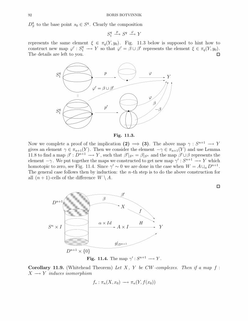
92 BORIS BOTVINNIK
DqS to the base point s0 ∈ Sq . Clearly the composition
Sq1p−→ Sq
ϕ−→ Y
represents the same element ξ ∈ πq(Y, y0). Fig. 11.3 below is supposed to hint how toconstruct new map ϕ′ : Sq1 −→ Y so that ϕ′ = β ∪ β ′ represents the element ξ ∈ πq(Y, y0).The details are left to you.
p ϕYSq1
Sq1
ϕ
p′β
−β
ϕ′ = β ∪ β′
Fig. 11.3.
Now we complete a proof of the implication (2) =⇒ (3). The above map γ : Sn+1 −→ Ygives an element γ ∈ πn+1(Y ). Then we consider the element −γ ∈ πn+1(Y ) and use Lemma11.8 to find a map β ′ : Dn+1 −→ Y , such that β ′|Sn = β|Sn and the map β ′∪β represents theelement −γ . We put together the maps we constructed to get new map γ′ : Sn+1 −→ Y whichhomotopic to zero, see Fig. 11.4. Since γ′ ∼ 0 we are done in the case when W = A∪αDn+1 .The general case follows then by induction: the n-th step is to do the above construction forall (n+ 1)-cells of the difference W \ A.
Dn+1 × 0
Dn+1
Sn × I A× Iα× Id H
Y
β′
X
β
f
g|Dn+1
Fig. 11.4. The map γ′ : Sn+1 −→ Y .
Corollary 11.9. (Whitehead Theorem) Let X , Y be CW -complexes. Then if a map f :X −→ Y induces isomorphism
f∗ : πn(X, x0) −→ πn(Y, f(x0))
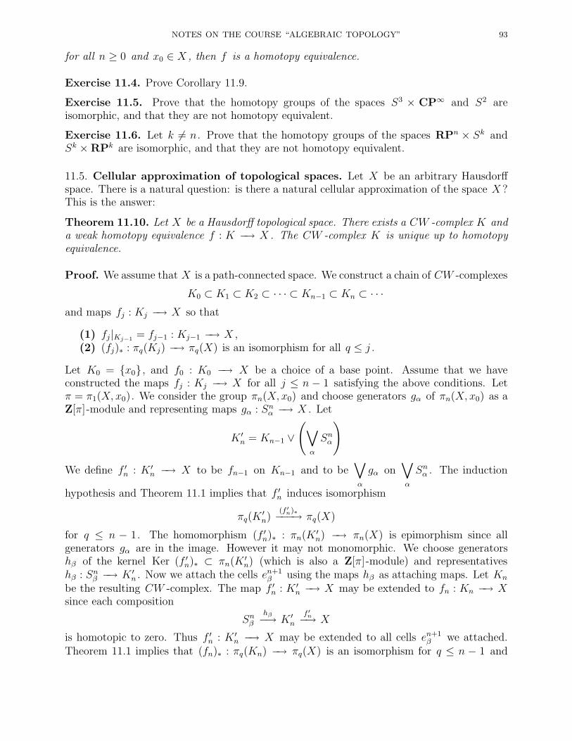
NOTES ON THE COURSE “ALGEBRAIC TOPOLOGY” 93
for all n ≥ 0 and x0 ∈ X , then f is a homotopy equivalence.
Exercise 11.4. Prove Corollary 11.9.
Exercise 11.5. Prove that the homotopy groups of the spaces S3 × CP∞ and S2 areisomorphic, and that they are not homotopy equivalent.
Exercise 11.6. Let k 6= n. Prove that the homotopy groups of the spaces RPn × Sk andSk ×RPk are isomorphic, and that they are not homotopy equivalent.
11.5. Cellular approximation of topological spaces. Let X be an arbitrary Hausdorffspace. There is a natural question: is there a natural cellular approximation of the space X ?This is the answer:
Theorem 11.10. Let X be a Hausdorff topological space. There exists a CW -complex K anda weak homotopy equivalence f : K −→ X . The CW -complex K is unique up to homotopyequivalence.
Proof. We assume that X is a path-connected space. We construct a chain of CW -complexes
K0 ⊂ K1 ⊂ K2 ⊂ · · · ⊂ Kn−1 ⊂ Kn ⊂ · · ·and maps fj : Kj −→ X so that
(1) fj|Kj−1= fj−1 : Kj−1 −→ X ,
(2) (fj)∗ : πq(Kj) −→ πq(X) is an isomorphism for all q ≤ j .
Let K0 = x0 , and f0 : K0 −→ X be a choice of a base point. Assume that we haveconstructed the maps fj : Kj −→ X for all j ≤ n − 1 satisfying the above conditions. Letπ = π1(X, x0). We consider the group πn(X, x0) and choose generators gα of πn(X, x0) as aZ[π]-module and representing maps gα : Snα −→ X . Let
K ′n = Kn−1 ∨
(∨
α
Snα
)
We define f ′n : K ′
n −→ X to be fn−1 on Kn−1 and to be∨
α
gα on∨
α
Snα . The induction
hypothesis and Theorem 11.1 implies that f ′n induces isomorphism
πq(K′n)
(f ′n)∗−−−→ πq(X)
for q ≤ n − 1. The homomorphism (f ′n)∗ : πn(K
′n) −→ πn(X) is epimorphism since all
generators gα are in the image. However it may not monomorphic. We choose generatorshβ of the kernel Ker (f ′
n)∗ ⊂ πn(K′n) (which is also a Z[π]-module) and representatives
hβ : Snβ −→ K ′n . Now we attach the cells en+1
β using the maps hβ as attaching maps. Let Kn
be the resulting CW -complex. The map f ′n : K ′
n −→ X may be extended to fn : Kn −→ Xsince each composition
Snβhβ−→ K ′
n
f ′n−→ X
is homotopic to zero. Thus f ′n : K ′
n −→ X may be extended to all cells en+1β we attached.
Theorem 11.1 implies that (fn)∗ : πq(Kn) −→ πq(X) is an isomorphism for q ≤ n − 1 and
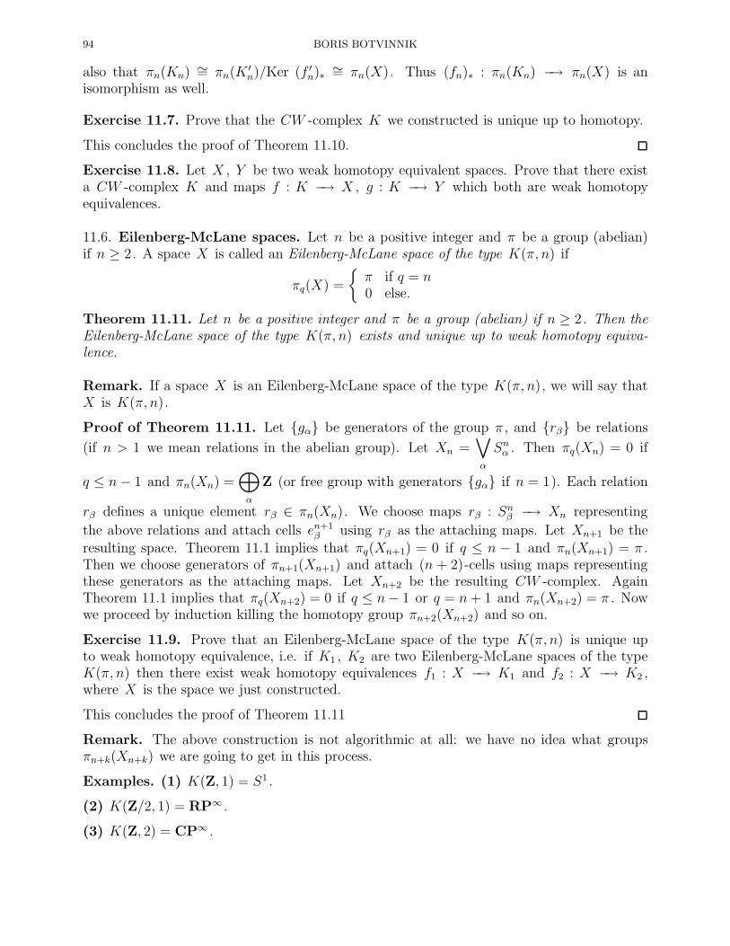
94 BORIS BOTVINNIK
also that πn(Kn) ∼= πn(K′n)/Ker (f ′
n)∗∼= πn(X). Thus (fn)∗ : πn(Kn) −→ πn(X) is an
isomorphism as well.
Exercise 11.7. Prove that the CW -complex K we constructed is unique up to homotopy.
This concludes the proof of Theorem 11.10.
Exercise 11.8. Let X , Y be two weak homotopy equivalent spaces. Prove that there exista CW -complex K and maps f : K −→ X , g : K −→ Y which both are weak homotopyequivalences.
11.6. Eilenberg-McLane spaces. Let n be a positive integer and π be a group (abelian)if n ≥ 2. A space X is called an Eilenberg-McLane space of the type K(π, n) if
πq(X) =
π if q = n0 else.
Theorem 11.11. Let n be a positive integer and π be a group (abelian) if n ≥ 2. Then theEilenberg-McLane space of the type K(π, n) exists and unique up to weak homotopy equiva-lence.
Remark. If a space X is an Eilenberg-McLane space of the type K(π, n), we will say thatX is K(π, n).
Proof of Theorem 11.11. Let gα be generators of the group π , and rβ be relations
(if n > 1 we mean relations in the abelian group). Let Xn =∨
α
Snα . Then πq(Xn) = 0 if
q ≤ n− 1 and πn(Xn) =⊕
α
Z (or free group with generators gα if n = 1). Each relation
rβ defines a unique element rβ ∈ πn(Xn). We choose maps rβ : Snβ −→ Xn representing
the above relations and attach cells en+1β using rβ as the attaching maps. Let Xn+1 be the
resulting space. Theorem 11.1 implies that πq(Xn+1) = 0 if q ≤ n − 1 and πn(Xn+1) = π .Then we choose generators of πn+1(Xn+1) and attach (n + 2)-cells using maps representingthese generators as the attaching maps. Let Xn+2 be the resulting CW -complex. AgainTheorem 11.1 implies that πq(Xn+2) = 0 if q ≤ n− 1 or q = n+ 1 and πn(Xn+2) = π . Nowwe proceed by induction killing the homotopy group πn+2(Xn+2) and so on.
Exercise 11.9. Prove that an Eilenberg-McLane space of the type K(π, n) is unique upto weak homotopy equivalence, i.e. if K1 , K2 are two Eilenberg-McLane spaces of the typeK(π, n) then there exist weak homotopy equivalences f1 : X −→ K1 and f2 : X −→ K2 ,where X is the space we just constructed.
This concludes the proof of Theorem 11.11
Remark. The above construction is not algorithmic at all: we have no idea what groupsπn+k(Xn+k) we are going to get in this process.
Examples. (1) K(Z, 1) = S1 .
(2) K(Z/2, 1) = RP∞ .
(3) K(Z, 2) = CP∞ .
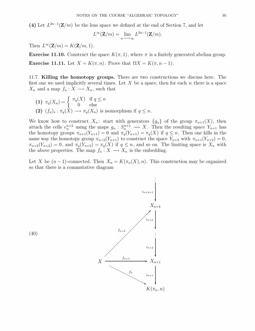
NOTES ON THE COURSE “ALGEBRAIC TOPOLOGY” 95
(4) Let L2n−1(Z/m) be the lens space we defined at the end of Section 7, and let
L∞(Z/m) = limn−→∞
L2n−1(Z/m).
Then L∞(Z/m) = K(Z/m, 1).
Exercise 11.10. Construct the space K(π, 1), where π is a finitely generated abelian group.
Exercise 11.11. Let X = K(π, n). Prove that ΩX = K(π, n− 1).
11.7. Killing the homotopy groups. There are two constructions we discuss here. Thefirst one we used implicitly several times. Let X be a space, then for each n there is a spaceXn and a map fn : X −→ Xn , such that
(1) πq(Xn) =
πq(X) if q ≤ n
0 else(2) (fn)∗ : πq(X) −→ πq(Xn) is isomorphism if q ≤ n.
We know how to construct Xn : start with generators gα of the group πn+1(X), thenattach the cells en+2
α using the maps gα : Sn+1α −→ X . Then the resulting space Yn+1 has
the homotopy groups πn+1(Yn+1) = 0 and πq(Yn+1) = πq(X) if q ≤ n. Then one kills in thesame way the homotopy group πn+2(Yn+1) to construct the space Yn+2 with πn+1(Yn+2) = 0,πn+2(Yn+2) = 0, and πq(Yn+2) = πq(X) if q ≤ n, and so on. The limiting space is Xn withthe above properties. The map fn : X −→ Xn is the embedding.
Let X be (n− 1)-connected. Then Xn = K(πn(X), n). This construction may be organizedso that there is a commutative diagram
(40)
...
?
in+k+1
Xn+k
?
in+k
...
?
in+2
X
fn+k
HHHHHHHHHj
fn
Xn+1
?
in+1
-fn+1
K(πn, n)

96 BORIS BOTVINNIK
where πq = πq(X). The maps iq : Xq −→ Xq−1 in the diagram (40) are homotopy equivalentto Serre fiber bundles, so that the diagram (40) becomes commutative up to homotopy. Let
Fq be the fiber of the Serre bundle Xqiq−→ Xq−1 . The exact sequence in homotopy
· · · −→ πj(Fq) −→ πj(Xq) −→ πj(Xq−1) −→ πj−1(Fq) −→ · · ·
for the Serre bundle Xqiq−→ Xq−1 immediately implies that Fq = K(πq, q) = ΩK(πq, q + 1).
Consider for a moment the Eileberg-McLane space K(π, q + 1). We have a canonical Serrefiber bundle π : E(K(π, q + 1)) → K(π, q + 1). It is easy to identify the fiber ΩK(π, q + 1)with the space K(π, q) (up to weak homotopy equivalence).
Here there is an important fact which we state without a proof:
Claim 11.1. Let p : E → B be a Serre fiber bundle with a fiber F = K(π, q). Then thereexists a map k : B → K(π, q+1), such that the following diagram commutes up to homotopy:
E
?
p
?
ΩK(π,q+1)
E(K(π, q + 1))
?
π
?
ΩK(π,q+1)
-k
B K(π, q + 1)-k
where we identify ΩK(π, q + 1) with K(π, q).
In particular, we obtain the following commutative diagram:
(41)
Xq
?
iq
?
ΩK(πq,q+1)
E(K(πq, q + 1))
?
p
?
ΩK(πq,q+1)
-kq
Xq−1 K(πq, q + 1)-kq
Here the maps kq : Xq−1 −→ K(πq+1, q + 2) are known as the Postnikov invariants of thespace X . In fact, the maps kq : Xq−1 −→ K(πq+1, q + 2) are defined up to homotopy anddetermine the elements in cohomology
kq ∈ Hq+2(X; πq+1), q ≥ n.
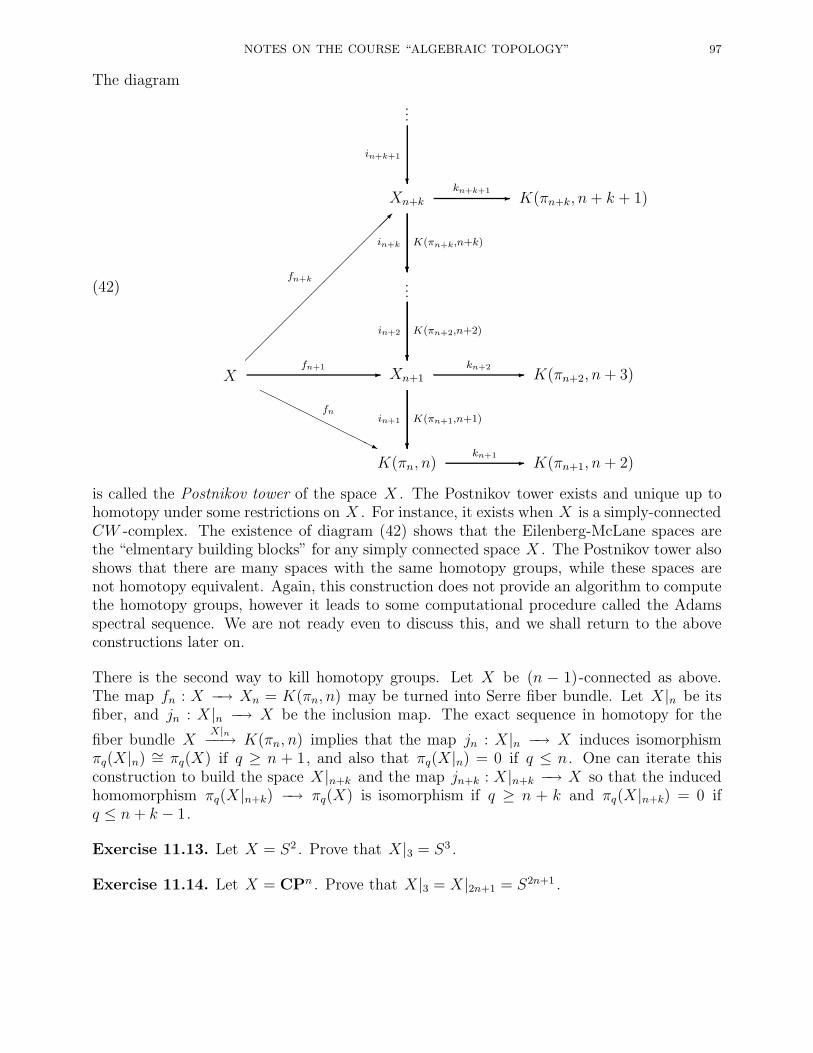
NOTES ON THE COURSE “ALGEBRAIC TOPOLOGY” 97
The diagram
(42)
...
?
in+k+1
Xn+k
?
in+k
?
K(πn+k,n+k)
K(πn+k, n+ k + 1)-kn+k+1
...
?
in+2
?
K(πn+2,n+2)
X
fn+k
HHHHHHHHHj
fn
Xn+1
?
in+1
?
K(πn+1,n+1)
K(πn+2, n+ 3)-fn+1 -kn+2
K(πn, n) K(πn+1, n+ 2)-kn+1
is called the Postnikov tower of the space X . The Postnikov tower exists and unique up tohomotopy under some restrictions on X . For instance, it exists when X is a simply-connectedCW -complex. The existence of diagram (42) shows that the Eilenberg-McLane spaces arethe “elmentary building blocks” for any simply connected space X . The Postnikov tower alsoshows that there are many spaces with the same homotopy groups, while these spaces arenot homotopy equivalent. Again, this construction does not provide an algorithm to computethe homotopy groups, however it leads to some computational procedure called the Adamsspectral sequence. We are not ready even to discuss this, and we shall return to the aboveconstructions later on.
There is the second way to kill homotopy groups. Let X be (n − 1)-connected as above.The map fn : X −→ Xn = K(πn, n) may be turned into Serre fiber bundle. Let X|n be itsfiber, and jn : X|n −→ X be the inclusion map. The exact sequence in homotopy for the
fiber bundle XX|n−−→ K(πn, n) implies that the map jn : X|n −→ X induces isomorphism
πq(X|n) ∼= πq(X) if q ≥ n + 1, and also that πq(X|n) = 0 if q ≤ n. One can iterate thisconstruction to build the space X|n+k and the map jn+k : X|n+k −→ X so that the inducedhomomorphism πq(X|n+k) −→ πq(X) is isomorphism if q ≥ n + k and πq(X|n+k) = 0 ifq ≤ n + k − 1.
Exercise 11.13. Let X = S2 . Prove that X|3 = S3 .
Exercise 11.14. Let X = CPn . Prove that X|3 = X|2n+1 = S2n+1 .

98 BORIS BOTVINNIK
12. Homology groups: basic constructions
The homotopy groups πq(X) are very important invariants. They are defined in the mostnatural way, and capture an important information about topological spaces. However it isvery difficult to compute the homotopy groups, as we have seen. There are just few finiteCW -complexes for which all homotopy groups are known. Even for the sphere Sn the problemto compute the homotopy groups is far from to be solved. Here we define different invariants:homology groups Hn(X) and cohomology groups Hn(X). These groups are much easier tocompute: we will be able to compute the homology groups for all basic examples. However,their definition requires more work.
12.1. Singular homology. We alredy defined the standard q -simplex:
∆q =
(t0, . . . , tq) | t0 ≥ 0, . . . , tq ≥ 0,
q∑
i=0
ti = 1
⊂ Rq+1.
Remark. Note that the standard simplex ∆q has vertices A0 = (1, 0, . . . , 0), A1 =(0, 1, 0, . . . , 0), . . . , Aq = (0, 0, . . . , 0, 1) in the space Rq+1 . In particular it defines the ori-entation of ∆q . The simplex ∆q has the i-th face (i = 0, . . . , q )
∆q−1(i) = (t0, . . . , tq) | ti = 0 which is a standard (q − 1)-simplex in the space
Rq(i) = (t0, . . . , tq) | ti = 0 ⊂ Rq+1
with the induced orientation.
A singular q -simplex of the space X is a continuous map f : ∆q −→ X . A singular q -chain isa finite linear combination
∑kifi , where each fi : ∆q −→ X is a singular q -simplex, ki ∈ Z.
The group q -chains Cq(X) is a free abelian group generated by all singular q -simplices of thespace X .
Now we define the “boundary homomorphism” ∂q : Cq(X) −→ Cq−1(X) as follows. Letf : ∆q −→ X be a singular simplex, then we denote Γi(f) = f |∆q−1(i) its restriction on thei-th face ∆q−1(i). We define:
∂qf =
q∑
i=0
(−1)iΓi(f).
Lemma 12.1. The composition
Cq+1(X)∂q+1−−−→ Cq(X)
∂q−→ Cq−1(X)
is trivial, i.e. Im ∂q+1 ⊂ Ker ∂q .
Proof. It follows from the definition and the identity:
(43) Γi(Γj(f)) =
Γj−1(Γi(f)) for j > i,Γj(Γi+1(f)) for j ≤ i.
Exercise 12.1. Check the identity (43) and complete the proof of Lemma 12.1.
NOTES ON THE COURSE “ALGEBRAIC TOPOLOGY” 99
Main Definition: The group Hq(X) = Ker ∂q/Im ∂q+1 is a q -th homology group of thespace X . (The group H0(X) = C0(x)/Im ∂1 , and Hq(X) = 0 for q < 0.)
The group Zq(X) = Ker ∂q is called the group of cycles, and the group Bq(X) = Im ∂q+1
the group of boundaries. Thus Hq(X) = Zq(X)/Bq(X). If c1, c2 ∈ Cq(X) are such elementsthat c1 − c2 = ∂q+1(d), then we say that the chain c1 is homologic to c2 . We call a class[c] ∈ Hq(X) a homological class of a cycle c.
The group Hq(X) is an abelian group; if it is finitely-generated, then Hq(X) ≡ Z⊕ . . .⊕Z⊕Zk1 ⊕ . . .⊕ Zkm
; the rank of this group (i.e. the number of Z’s in this decomposition) is theBetti number of the space X .
12.2. Chain complexes, chain maps and chain homotopy. A chain complex C is asequence of abelian groups and homomorphisms
(44) . . . −→ Cq+1∂q+1−−−→ Cq
∂q−→ Cq−1 −→ . . . −→ C1∂1−→ C0 −→ 0 ,
such that ∂q ∂q+1 = 0 for all q ≥ 1. For a given chain complex C the group Hq(C) =Ker ∂q/Im ∂q+1 is the q -th homology group of C . The chain complex
(45) . . . −→ Cq+1(X)∂q+1−−−→ Cq(X)
∂q−→ Cq−1(X) −→ . . . −→ C1(X)∂1−→ C0(X) −→ 0 ,
will be denoted as C(X). Thus Hq(X) = Hq(C(X)).
Let C′ , C′′ be two chain complexes. A chain map ϕ : C′ −→ C′′ is a collection of homomor-phisms ϕq : C ′
q −→ C ′′q such that the diagram
(46)
. . . C ′q
?
ϕq
C ′q−1
?
ϕq−1
. . . C ′1
?
ϕ1
C ′0
?
ϕ0
0-∂′q+1 -
∂′q -∂′q−1 - -
∂′1 -
. . . C ′′q C ′′
q−1. . . C ′′
1 C ′′0 0-
∂′′q+1 -∂′′q -
∂′′q−1 - -∂′′1 -
commutes. It is clear that a chain map ϕ : C′ −→ C′′ induces the homomorphisms ϕ∗ :Hq(C′) −→ Hq(C′′). In particular, a map g : X −→ Y induces the homomorphism g# :Cq(X) −→ Cq(Y ) (which maps a singular simplex f : ∆q −→ X to a singular simplexg f : ∆q −→ Y ). It defines a chain map g# : C(X) −→ C(Y ) and homomorphismsg∗ : Hq(X) −→ Hq(Y ).
Exercise 12.2. Prove the following statements:1. Let g : X −→ Y , h : Y −→ Z be two maps. Then (hg)# = h#g# , and (hg)∗ = h∗g∗ .2. Let i : X −→ X be the identity map. Then i∗ = Id .
Let ϕ, ψ : C′ −→ C′′ be two chain maps. We say the ϕ, ψ are chain homotopic if there arehomomorphisms Dq : C ′
q −→ C ′′q−1 such that for each q
Dq−1 ∂′q + ∂′′q+1 Dq = ϕq − ψq,(here D−1 = 0). In that case we will write down ϕ ∼ ψ .
Theorem 12.2. Let ϕ, ψ : C′ −→ C′′ be two chain maps, and ϕ ∼ ψ . Then
ϕ∗ = ψ∗ : Hq(C′) −→ Hq(C′′).

100 BORIS BOTVINNIK
Exercise 12.3. Prove Theorem 12.2.
Theorem 12.3. Let g, h : X −→ Y be homotopic maps, then g∗ = h∗ : Hq(X) −→ Hq(Y ).In other words, homotopic maps induce the same homomorphism in homology groups.
Proof. By definition we have a homotopy H : X × I −→ Y , such that H|X×0 = g ,H|X×1 = h. Then for any singular simplex f : ∆q −→ X we have a map H (f × I) :∆q× I −→ Y . The cylinder ∆q× I has a canonical simplicial structure: we subdivide ∆q× Iinto (q + 1)-simplices ∆
q+1(i), i = 0, . . . , q , as follows:
∆q+1
(i) = (t0, . . . , tq, τ) ∈ ∆q × I | t0 + . . .+ ti−1 ≤ τ ≤ t0 + . . .+ ti ,see Fig. 12.1. for q = 1, 2:
(1,0) (0,1) (1,0,0)
(0,1,0)
(0,0,1)
Fig. 12.1.
The map G = H (f × I) : ∆q × I −→ Y defines (q + 1) singular simplices of dimension(q + 1). We define
D(f) =
q∑
i=0
(−1)iG|∆
q+1(i).
It is easy to check that the homomorphisms
Dq : Cq(X) −→ Cq+1(Y ), Dq
(∑kifi
)=∑
kiDq(fi)
define a chain homotopy D : C(X) −→ C(Y ).
Corollary 12.4. Let X and Y be homotopy equivalent spaces. Then Hq(X) ∼= Hq(Y ) forall q .
Remark. There is a natural question: what happens if X and Y are weak homotopyequivalent? We will find the answer on this question in the next section.
12.3. First computations. By definition, the groups Cq(X) are really huge, and it is dif-ficult to compute homology directly. We will learn how to do this in a while, however evennow we can prove several important facts.
Let ∗ be a space consisting of a single point. Clearly there is a unique map fq : ∆q −→ ∗for any q . We have that Cq(∗) = Z for all q ≥ 0. By definition, ∂q(fq) =
∑(−1)iΓi(fq) =
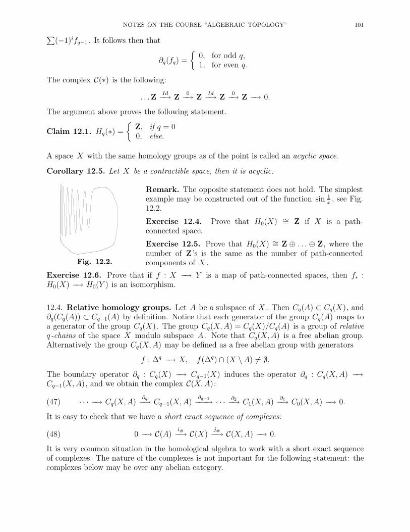
NOTES ON THE COURSE “ALGEBRAIC TOPOLOGY” 101
∑(−1)ifq−1 . It follows then that
∂q(fq) =
0, for odd q,1, for even q.
The complex C(∗) is the following:
. . .ZId−→ Z
0−→ ZId−→ Z
0−→ Z −→ 0.
The argument above proves the following statement.
Claim 12.1. Hq(∗) =
Z, if q = 00, else.
A space X with the same homology groups as of the point is called an acyclic space.
Corollary 12.5. Let X be a contractible space, then it is acyclic.
Fig. 12.2.
Remark. The opposite statement does not hold. The simplestexample may be constructed out of the function sin 1
x, see Fig.
12.2.
Exercise 12.4. Prove that H0(X) ∼= Z if X is a path-connected space.
Exercise 12.5. Prove that H0(X) ∼= Z ⊕ . . . ⊕ Z, where thenumber of Z’s is the same as the number of path-connectedcomponents of X .
Exercise 12.6. Prove that if f : X −→ Y is a map of path-connected spaces, then f∗ :H0(X) −→ H0(Y ) is an isomorphism.
12.4. Relative homology groups. Let A be a subspace of X . Then Cq(A) ⊂ Cq(X), and∂q(Cq(A)) ⊂ Cq−1(A) by definition. Notice that each generator of the group Cq(A) maps toa generator of the group Cq(X). The group Cq(X,A) = Cq(X)/Cq(A) is a group of relativeq -chains of the space X modulo subspace A. Note that Cq(X,A) is a free abelian group.Alternatively the group Cq(X,A) may be defined as a free abelian group with generators
f : ∆q −→ X, f(∆q) ∩ (X \A) 6= ∅.The boundary operator ∂q : Cq(X) −→ Cq−1(X) induces the operator ∂q : Cq(X,A) −→Cq−1(X,A), and we obtain the complex C(X,A):
(47) · · · −→ Cq(X,A)∂q−→ Cq−1(X,A)
∂q−1−−−→ · · · ∂2−→ C1(X,A)∂1−→ C0(X,A) −→ 0.
It is easy to check that we have a short exact sequence of complexes:
(48) 0 −→ C(A)i#−→ C(X)
j#−→ C(X,A) −→ 0.
It is very common situation in the homological algebra to work with a short exact sequenceof complexes. The nature of the complexes is not important for the following statement: thecomplexes below may be over any abelian category.

102 BORIS BOTVINNIK
Lemma 12.6. (LES-Lemma) Let 0 −→ C′ i−→ C −→ C′′ −→ 0 be a short exact sequence ofcomplexes. Then there is a long exact sequence of homology groups
(49) · · · −→ Hq(C′) i∗−→ Hq(C) j∗−→ Hq(C′′) ∂−→ Hq−1(C′) i∗−→ · · ·where the homomorphisms i∗ and j∗ are induced by i and j respectively, and ∂ is the boundaryhomorphism to be defined.
Proof. First we define the boundary homomorphism ∂ : Hq(C′′) −→ Hq−1(C′). We have thefollowing commutative diagram:
(50)
0 C ′q+1
?
∂′q+1
Cq+1
?
∂q+1
C ′′q+1
?
∂′′q+1
0- -iq+1 -
jq+1 -
0 C ′q
?
∂′q
Cq
?
∂q
C ′′q
?
∂′′q
0- -iq -jq -
0 C ′q−1 Cq−1 C ′′
q−1 0- -iq−1 -
jq−1 -
Let α ∈ Hq(C′′), and c′′ ∈ Ker ∂′′q such that α = [c′′]. Choose an element c ∈ Cq such thatjq(c) = c′′ , then the element c = ∂q(c) ∈ Cq−1 is such that jq−1(c) = 0 by commutativity of(50). The exactness of the bottom row gives that there exists an element c′ ∈ C ′
q−1 such thatiq(c
′) = c.
Now we notice that c′ ∈ Ker ∂′q−1 : it follows from the commutative diagram
(51)
0 C ′q−1
?
∂′q−1
Cq−1
?
∂q−1
C ′′q−1
?
∂′′q−1
0- -iq−1 -
jq−1 -
0 C ′q−2 Cq−2 C ′′
q 0- -iq−2 -
jq−2 -
since iq−1 is monomorphism, c = ∂q(c), and
iq−1 ∂′q−1(c′) = ∂q−1 iq(c) = ∂q−1 ∂q(c) = 0.
Thus c′ ∈ Ker ∂q−1 , and we define ∂(α) = [c′] ∈ Hq−1(C′).Exercise 12.7. Prove that the homomorphism ∂ : Hq(C′′) −→ Hq−1(C′) is well-defined.
The proof that the sequence (49) is exact is rather routine exercise. We will prove only theexactness at the term Hq(C′′), i.e. that Im j∗ = Ker ∂ .
The inclusion Im j∗ ⊂ Ker ∂ follows immediately from the definition. Now we prove thatKer ∂ ⊂ Im j∗ . Let α ∈ Ker ∂ . As above (in the definition of ∂ ) we consider a cycle c′′ ∈ C ′′
q ,an element c , such that jq(c) = c′′ , then the element c = ∂q(c), and, finally, the element c′
such that iq−1(c′) = c. We know that [c′] = 0, i.e. c′ ∈ Im ∂q . Let b′ ∈ C ′
q be such that
NOTES ON THE COURSE “ALGEBRAIC TOPOLOGY” 103
∂q(b′) = c′ . Let c1 = iq(b
′). By commutativity of (50) ∂q(c − c1) = 0, and by exatness ofthe second row of (50) jq(c − c1) = c′′ . Thus the element d = c − c1 ∈ Cq is a cycle, andjq(d) = c′′ , and j∗([d]) = α .
Exercise 12.8. Prove the exactness of (49) at the term Hq(C′).The exactness of (49) at the term Hq(C) is an easy exercise.
Now we specify Lemma 12.6 in the case of the exact sequence of complexes
0 −→ C(A)i#−→ C(X)
j#−→ C(X,A) −→ 0.
The boundary operator ∂q : Cq(X,A) −→ Cq−1(X,A) is induced by the boundary operator∂q : Cq(X) −→ Cq−1(X), and clearly ∂q(c) ∈ Cq−1(A) if c ∈ Cq−1(X,A) is a cycle.
Corollary 12.7. Let (X,A) be a pair of spaces. Then there is an exact sequence of homologygroups:
(52) · · · ∂−→ Hq(A)i∗−→ Hq(X)
j∗−→ Hq(X,A)∂−→ Hq−1(A)
i∗−→ · · · .
Let B ⊂ A ⊂ X be a triple of spaces. We have the following maps of pairs:
(53) (A,B)i−→ (X,B)
j−→ (X,A)
which induce the homomorphisms C(A,B)i#−→ C(X,B)
j#−→ C(X,A).
Exercise 12.9. Prove that the sequence of complexes
(54) 0 −→ C(A,B)i#−→ C(X,B)
j#−→ C(X,A) −→ 0
is exact.
Exercise 12.9 and the LES-Lemma imply the following result.
Corollary 12.8. Let B ⊂ A ⊂ X be a triple of spaces. Then there is a long exact sequencein homology:
(55) · · · −→ Hq(A,B)i∗−→ Hq(X,B)
j∗−→ Hq(X,A)∂−→ Hq−1(A,B)
i∗−→ · · · .
The relative homology groups are natural invariant.
Exercise 12.10. Let B ⊂ A ⊂ X and B′ ⊂ A′ ⊂ X ′ be two triples of spaces, andf : X −→ X ′ be such a map that f(B) ⊂ B′ , and f(A) ⊂ A′ . Prove that the followingdiagram commutes:
· · · Hq(A,B)
?
f∗
Hq(X,B)
?
f∗
Hq(X,A)
?
f∗
Hq−1(A,B)
?
f∗
· · ·- -i∗ -j∗ -∂ -
· · · Hq(A′,B′) Hq(X
′,B′) Hq(X′,A′) Hq−1(A
′,B′) · · ·- -i∗ -j∗ -∂ -
Exercise 12.11. Let f : (X,A) −→ (X ′, A′) be such map of pairs that the induced mapsf : X −→ X ′ and f |A : A −→ A′ are homotopy equivalences. Prove that f∗ : Hq(X,A) −→Hq(X
′, A′) is an isomorphism for each q .
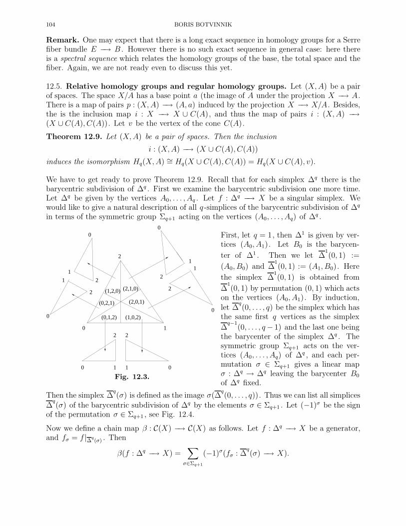
104 BORIS BOTVINNIK
Remark. One may expect that there is a long exact sequence in homology groups for a Serrefiber bundle E −→ B . However there is no such exact sequence in general case: here thereis a spectral sequence which relates the homology groups of the base, the total space and thefiber. Again, we are not ready even to discuss this yet.
12.5. Relative homology groups and regular homology groups. Let (X,A) be a pairof spaces. The space X/A has a base point a (the image of A under the projection X −→ A.There is a map of pairs p : (X,A) −→ (A, a) induced by the projection X −→ X/A. Besides,the is the inclusion map i : X −→ X ∪ C(A), and thus the map of pairs i : (X,A) −→(X ∪ C(A), C(A)). Let v be the vertex of the cone C(A).
Theorem 12.9. Let (X,A) be a pair of spaces. Then the inclusion
i : (X,A) −→ (X ∪ C(A), C(A))
induces the isomorphism Hq(X,A) ∼= Hq(X ∪ C(A), C(A)) = Hq(X ∪ C(A), v).
We have to get ready to prove Theorem 12.9. Recall that for each simplex ∆q there is thebarycentric subdivision of ∆q . First we examine the barycentric subdivision one more time.Let ∆q be given by the vertices A0, . . . , Aq . Let f : ∆q −→ X be a singular simplex. Wewould like to give a natural description of all q -simplices of the barycentric subdivision of ∆q
in terms of the symmetric group Σq+1 acting on the vertices (A0, . . . , Aq) of ∆q .
0 1
2
1 0
2
0
2
1
2
1
00
1
2
0
1
2
0 1
2
(0,1,2) (1,0,2)
(2,0,1)
(2,1,0)(1,2,0)
(0,2,1)
Fig. 12.3.
First, let q = 1, then ∆1 is given by ver-tices (A0, A1). Let B0 is the barycen-
ter of ∆1 . Then we let ∆1(0, 1) :=
(A0, B0) and ∆1(0, 1) := (A1, B0). Here
the simplex ∆1(0, 1) is obtained from
∆1(0, 1) by permutation (0, 1) which acts
on the vertices (A0, A1). By induction,let ∆
q(0, . . . , q) be the simplex which has
the same first q vertices as the simplex
∆q−1
(0, . . . , q− 1) and the last one beingthe barycenter of the simplex ∆q . Thesymmetric group Σq+1 acts on the ver-tices (A0, . . . , Aq) of ∆q , and each per-mutation σ ∈ Σq+1 gives a linear mapσ : ∆q → ∆q leaving the barycenter B0
of ∆q fixed.
Then the simplex ∆q(σ) is defined as the image σ(∆
q(0, . . . , q)). Thus we can list all simplices
∆q(σ) of the barycentric subdivision of ∆q by the elements σ ∈ Σq+1 . Let (−1)σ be the sign
of the permutation σ ∈ Σq+1 , see Fig. 12.4.
Now we define a chain map β : C(X) −→ C(X) as follows. Let f : ∆q −→ X be a generator,and fσ = f |∆q
(σ) . Then
β(f : ∆q −→ X) =∑
σ∈Σq+1
(−1)σ(fσ : ∆q(σ) −→ X).
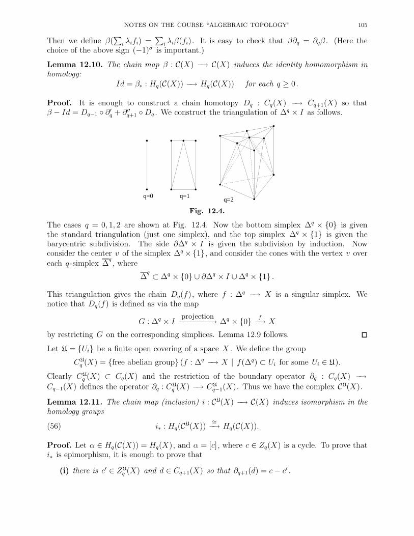
NOTES ON THE COURSE “ALGEBRAIC TOPOLOGY” 105
Then we define β(∑
i λifi) =∑
i λiβ(fi). It is easy to check that β∂q = ∂qβ . (Here thechoice of the above sign (−1)σ is important.)
Lemma 12.10. The chain map β : C(X) −→ C(X) induces the identity homomorphism inhomology:
Id = β∗ : Hq(C(X)) −→ Hq(C(X)) for each q ≥ 0.
Proof. It is enough to construct a chain homotopy Dq : Cq(X) −→ Cq+1(X) so thatβ − Id = Dq−1 ∂′q + ∂′′q+1 Dq . We construct the triangulation of ∆q × I as follows.
q=0 q=1q=2
Fig. 12.4.
The cases q = 0, 1, 2 are shown at Fig. 12.4. Now the bottom simplex ∆q × 0 is giventhe standard triangulation (just one simplex), and the top simplex ∆q × 1 is given thebarycentric subdivision. The side ∂∆q × I is given the subdivision by induction. Nowconsider the center v of the simplex ∆q ×1 , and consider the cones with the vertex v overeach q -simplex ∆
q, where
∆q ⊂ ∆q × 0 ∪ ∂∆q × I ∪∆q × 1 .
This triangulation gives the chain Dq(f), where f : ∆q −→ X is a singular simplex. Wenotice that Dq(f) is defined as via the map
G : ∆q × I projection−−−−−−−→ ∆q × 0 f−→ X
by restricting G on the corresponding simplices. Lemma 12.9 follows.
Let U = Ui be a finite open covering of a space X . We define the group
CU
q (X) = free abelian group (f : ∆q −→ X | f(∆q) ⊂ Ui for some Ui ∈ U).
Clearly CU
q (X) ⊂ Cq(X) and the restriction of the boundary operator ∂q : Cq(X) −→Cq−1(X) defines the operator ∂q : CU
q (X) −→ CU
q−1(X). Thus we have the complex CU(X).
Lemma 12.11. The chain map (inclusion) i : CU(X) −→ C(X) induces isomorphism in thehomology groups
(56) i∗ : Hq(CU(X))∼=−→ Hq(C(X)).
Proof. Let α ∈ Hq(C(X)) = Hq(X), and α = [c], where c ∈ Zq(X) is a cycle. To prove thati∗ is epimorphism, it is enough to prove that
(i) there is c′ ∈ ZU
q (X) and d ∈ Cq+1(X) so that ∂q+1(d) = c− c′ .
106 BORIS BOTVINNIK
Let α′ ∈ Hq(CU(X)), α′ = [c′], where c′ ∈ ZU
q (X). Assume that i∗(α′) = 0, i.e. c′ = ∂q+1d
where d ∈ Cq+1(X). To prove that i∗ is monomorphism, it is enough to show that
(ii) there is d′ ∈ CU
q+1(X) such that ∂q+1(d′) = c′ .
The above statements follow from the following three observations:
(1) For any c ∈ Cq(X) there is n ≥ 1 so that βnc ∈ CU
q (X).(2) For any c ∈ Cq(X) and n ≥ 1 there is d ∈ Cq(X) such that ∂q+1(d) = c − βnc.
(Lemma 12.10.)(3) Let c′ ∈ ZU
q (X), then for any n ≥ 1 there is d′ ∈ CU
q+1(X) such that ∂q+1d = c′−βnc′ .
Exercise 12.12. Prove the properties (1) and (3).
Exercise 12.13. Show that the above statements (i), (ii) follow from (1), (2), (3).
This concludes the proof.
Remark. Let V = Vj be a finite covering of X , such that X =⋃
j
o
V j , whereo
V is
the interior of V . Then the chain map CV(X) −→ C(X) also induces isomorphism in thehomology groups.
Remark. Let (X,A) be a pair of spaces. Then a covering U = Uj induces a coveringUj ∩ A . We denote a corresponding chain complex by CV(A). Then for each q we have ashort exact sequence
0→ CV
q (A) −→ CV
q (X) −→ CV
q (X,A)→ 0
which determines the relative chain complex CV(X,A). It easy to modify the proof of Lemma12.11 (and use five-lemma) to show that the natural chain map CV(X,A) −→ C(X,A) inducesan isomorphism in the homology groups
Hq(CV(X,A))∼=−→ Hq(C(X,A)) = Hq(X,A).
Proof of Theorem 12.9. Consider the following covering of the space X ∪ C(A).Let U1 = (X ∪ C(A)) \ X and U2 = X ∪ C(A), where C(A) is the half-cone over A, i.e.C(A) = (a, t) ∈ C(A) | 0 ≤ t < 1/2 . The relative version of Lemma 12.11 (see the aboveremark) implies that the embedding
CU(X ∪ C(A), C(A)) −→ C(X ∪ C(A), C(A))
induces an isomorphism in the homology groups. By definition of a relative chain complex,we have the isomorphism:
CU
q(X ∪ C(A), C(A))∼=CU
q(X ∪ C(A))/CU
q (C(A)).
Then we observe that there is an isomorphism
CU
q (X ∪ C(A))/CU
q (C(A)) ∼= Cq(X ∪ C(A))/Cq(C(A)) = Cq(X ∪ C(A), C(A)).

NOTES ON THE COURSE “ALGEBRAIC TOPOLOGY” 107
Fig. 12.5.
Indeed, let f : ∆q → X ∪ C(A) be a generator in CU
q (X ∪ C(A), C(A)), i.e.
f(∆q) ∩ (X ∪ C(A) \ C(A)) 6= ∅and f(∆q) ⊂ U1 or f(∆q) ⊂ U2 . Since U1 = (X ∪ C(A)) \X , f(∆q) ⊂ U2 = X ∪ C(A) andf(∆q) ∩ C(A) = ∅ , the map f : ∆q → X ∪ C(A) is a generator of the free abelian group
Cq(X ∪ C(A), C(A)) = Cq(X ∪ C(A))/Cq(C(A)).
It is also easy to check that any generator in Cq(X ∪ C(A))/Cq(C(A)) gives a generator inthe group CU
q (X ∪ C(A), C(A)).
Since X ∪ C(A) is homotopy equivalent to X , and C(A) ∼ A, we obtain the isomorphisms
Hq(X ∪ C(A), C(A)) ∼= Hq(X ∪ C(A), C(A)) ∼= Hq(X,A).
This concludes the proof of Theorem 12.9.
Corollary 12.12. Let (X,A) be a Borsuk pair. Then the projection p : (X,A) −→ (A, a)induces the isomorphism p∗ : Hq(X,A) −→ Hq(X/A, a) for each q .
Exercise 12.14. Prove Corollary 12.12.
12.6. Excision Theorem. Let (X,A) be a pair of spaces, and B ⊂ A. The map of pairse : (X \B,A \B) −→ (A,B) induces the excision homomorphism:
(57) e∗ : Hq(X \B,A \B) −→ Hq(X,A)
The following result is known as the Excision Theorem.
Theorem 12.13. Let (X,A) be a pair of Hausdorff spaces, and B ⊂ A so that B ⊂o
A.Then the homomorphism e∗ : Hq(X \B,A \B) −→ Hq(X,A) is an isomorphism.
Proof. We use the condition B ⊂o
A to notice thato
(X \B) ⊃ X \B ⊃ X \o
A.
Thuso
A ∪o
(X \B) = X . We consider the covering V = V1, V2 of X , where V1 = A,V2 = X \ B . The chain complex CV(X) (see the remark following Exercise 12.13) gives thechain map i : CV(X) −→ C(X). Note that for each q
CV
q (X) ∼= Cq(A) + Cq(X \B) ⊂ Cq(X).
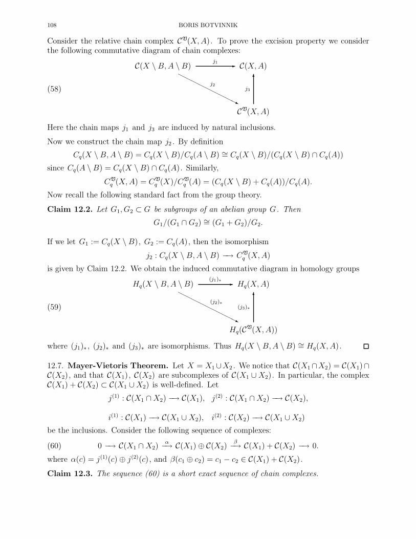
108 BORIS BOTVINNIK
Consider the relative chain complex CV(X,A). To prove the excision property we considerthe following commutative diagram of chain complexes:
(58)
C(X \B,A \B)HHHHHHHHHj
j2
C(X,A)-j1
CV(X,A)
6j3
Here the chain maps j1 and j3 are induced by natural inclusions.
Now we construct the chain map j2 . By definition
Cq(X \B,A \B) = Cq(X \B)/Cq(A \B) ∼= Cq(X \B)/(Cq(X \B) ∩ Cq(A))
since Cq(A \B) = Cq(X \B) ∩ Cq(A). Similarly,
CV
q (X,A) = CV
q (X)/CV
q (A) = (Cq(X \B) + Cq(A))/Cq(A).
Now recall the following standard fact from the group theory.
Claim 12.2. Let G1, G2 ⊂ G be subgroups of an abelian group G. Then
G1/(G1 ∩G2) ∼= (G1 +G2)/G2.
If we let G1 := Cq(X \B), G2 := Cq(A), then the isomorphism
j2 : Cq(X \B,A \B) −→ CV
q (X,A)
is given by Claim 12.2. We obtain the induced commutative diagram in homology groups
(59)
Hq(X \B,A \B)HHHHHHHHHj
(j2)∗
Hq(X,A)-(j1)∗
Hq(CV(X,A))
6(j3)∗
where (j1)∗ , (j2)∗ and (j3)∗ are isomorphisms. Thus Hq(X \B,A \B) ∼= Hq(X,A).
12.7. Mayer-Vietoris Theorem. Let X = X1∪X2 . We notice that C(X1∩X2) = C(X1)∩C(X2), and that C(X1), C(X2) are subcomplexes of C(X1 ∪X2). In particular, the complexC(X1) + C(X2) ⊂ C(X1 ∪X2) is well-defined. Let
j(1) : C(X1 ∩X2) −→ C(X1), j(2) : C(X1 ∩X2) −→ C(X2),
i(1) : C(X1) −→ C(X1 ∪X2), i(2) : C(X2) −→ C(X1 ∪X2)
be the inclusions. Consider the following sequence of complexes:
(60) 0 −→ C(X1 ∩X2)α−→ C(X1)⊕ C(X2)
β−→ C(X1) + C(X2) −→ 0.
where α(c) = j(1)(c)⊕ j(2)(c), and β(c1 ⊕ c2) = c1 − c2 ∈ C(X1) + C(X2).
Claim 12.3. The sequence (60) is a short exact sequence of chain complexes.
NOTES ON THE COURSE “ALGEBRAIC TOPOLOGY” 109
Exercise 12.15. Prove Claim 12.3.
Lemma 12.14. Let X1, X2 ⊂ X , and X1 ∪ X2 = X ,o
X1 ∪o
X2 = X . Then the chain mapC(X1) + C(X2) −→ C(X1 ∪X2) induces isomorphism in the homology groups.
Proof. Consider the covering V = X1, X2 . Then by definition CV(X1 ∪ X2) = C(X1) +C(X2). Lemma 12.11 and the remark following Lemma 12.11 completes the proof.
Theorem 12.15. (Mayer-Vietoris Theorem) Let X be a space, and X = X1 ∪ X2 , and
X =o
X1 ∪o
X2 . Then there is a long exact sequence
(61) · · · → Hq(X1 ∩X2)α∗−→ Hq(X1)⊕Hq(X2)
β∗−→ Hq(X1 ∪X2)∂−→ Hq−1(X1 ∩X2)→ · · ·
This is the Mayer-Vietoris long exact sequence.
Proof. The short exact sequence of chain complexes (60) induces the long exact sequnce
· · · → Hq(C(X1 ∩X2))α∗−→ Hq(C(X1))⊕Hq(C(X2))
β∗−→ Hq(C(X1) + C(X2))
∂−→ Hq−1(C(X1 ∩X2))α∗−→ Hq−1(C(X1))⊕Hq−1(C(X2))→ · · ·
To complete the proof we replace the groups Hq(C(X1)+C(X2)) by Hq(X1∪X2) using Lemma12.14.
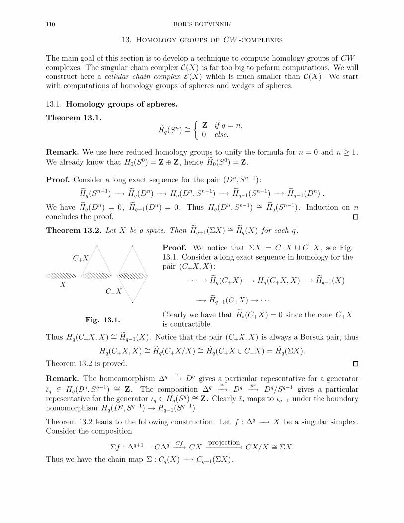
110 BORIS BOTVINNIK
13. Homology groups of CW -complexes
The main goal of this section is to develop a technique to compute homology groups of CW -complexes. The singular chain complex C(X) is far too big to peform computations. We willconstruct here a cellular chain complex E(X) which is much smaller than C(X). We startwith computations of homology groups of spheres and wedges of spheres.
13.1. Homology groups of spheres.
Theorem 13.1.
Hq(Sn) ∼=
Z if q = n,0 else.
Remark. We use here reduced homology groups to unify the formula for n = 0 and n ≥ 1.
We already know that H0(S0) = Z⊕ Z, hence H0(S
0) = Z.
Proof. Consider a long exact sequence for the pair (Dn, Sn−1):
Hq(Sn−1) −→ Hq(D
n) −→ Hq(Dn, Sn−1) −→ Hq−1(S
n−1) −→ Hq−1(Dn) .
We have Hq(Dn) = 0, Hq−1(D
n) = 0. Thus Hq(Dn, Sn−1) ∼= Hq(S
n−1). Induction on nconcludes the proof.
Theorem 13.2. Let X be a space. Then Hq+1(ΣX) ∼= Hq(X) for each q .
X
C+X
C−X
Fig. 13.1.
Proof. We notice that ΣX = C+X ∪ C−X , see Fig.13.1. Consider a long exact sequence in homology for thepair (C+X,X):
· · · → Hq(C+X) −→ Hq(C+X,X) −→ Hq−1(X)
−→ Hq−1(C+X)→ · · ·Clearly we have that H∗(C+X) = 0 since the cone C+Xis contractible.
Thus Hq(C+X,X) ∼= Hq−1(X). Notice that the pair (C+X,X) is always a Borsuk pair, thus
Hq(C+X,X) ∼= Hq(C+X/X) ∼= Hq(C+X ∪ C−X) = Hq(ΣX).
Theorem 13.2 is proved.
Remark. The homeomorphism ∆q∼=−→ Dq gives a particular repesentative for a generator
ιq ∈ Hq(Dq, Sq−1) ∼= Z. The composition ∆q
∼=−→ Dq pr−→ Dq/Sq−1 gives a particularrepesentative for the generator ιq ∈ Hq(S
q) ∼= Z. Clearly ιq maps to ιq−1 under the boundaryhomomorphism Hq(D
q, Sq−1)→ Hq−1(Sq−1).
Theorem 13.2 leads to the following construction. Let f : ∆q −→ X be a singular simplex.Consider the composition
Σf : ∆q+1 = C∆q Cf−−→ CXprojection−−−−−−−→ CX/X ∼= ΣX.
Thus we have the chain map Σ : Cq(X) −→ Cq+1(ΣX).

NOTES ON THE COURSE “ALGEBRAIC TOPOLOGY” 111
Excercise 13.1. Show that the map Σ : Cq(X) −→ Cq+1(ΣX) commutes with the boundary
operator and induces the isomorphism Σ : Hq(X) −→ Hq+1(ΣX).
13.2. Homology groups of a wedge.
Theorem 13.3. Let A be a set of indices, and Snα be a copy of the n-th sphere, α ∈ A.Then
Hq
(∨
α∈ASnα
)=
⊕
α∈AZ(α), if q = n,
0, else.
Here⊕
α∈AZ(α) is a free abelian group with generators α ∈ A.
This result follows from Theorem 13.2 because of the homotopy equivalence
Σ
(∨
α∈ASnα
)∼∨
α∈AΣSnα =
∨
α∈ASn+1α .
On the other hand Theorem 13.3 is a particular case in the following result.
Theorem 13.4. Let (Xα, xα) be based spaces, α ∈ A. Assume that the pair (Xα, xα) isBorsuk pair for each α ∈ A. Then
Hq
(∨
α∈AXα
)=⊕
α∈AHq(Xα).
Excercise 13.2. Prove Theorem 13.4. Hint: The wedge∨
α∈AXα is a factor-space of the
disjoint union⊔
α∈AXα by the union of the base points.
13.3. Maps g :∨
α∈ASnα→
∨
β∈BSnβ . Let f : Sn −→ Sn be a map. Then the homotopy class
[f ] = dιn , where d ∈ Z, and ιn ∈ πn(Sn) is a generator represented by the identity map
Sn −→ Sn . Recall that d = deg f .
Claim 13.1. Let f : Sn −→ Sn be a map of degree d = deg f . Then the induced homomor-phism f∗ : Hn(S
n) −→ Hn(Sn) is multiplication by d.
Proof. We constructed earlier a map g(d) : Sn −→ Sn of the degree d :
g1 g2
Fig. 13.2.
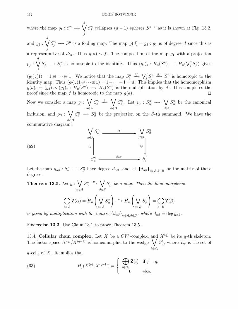
112 BORIS BOTVINNIK
where the map g1 : Sn −→d∨
j
Snj collapses (d− 1) spheres Sn−1 as it is shown at Fig. 13.2,
and g2 :d∨
j
Snj −→ Sn is a folding map. The map g(d) = g2 g1 is of degree d since this is
a representative of dιn . Thus g(d) ∼ f . The composition of the map g1 with a projection
pj :d∨
j
Snj −→ Snj is homotopic to the identinty. Thus (g1)∗ : Hn(Sn) −→ Hn(
∨dj S
nj ) gives
(g1)∗(1) = 1 ⊕ · · · ⊕ 1. We notice that the map Snjij−→ ∨d
j Snj
g2−→ Sn is homotopic to the
identity map. Thus (g2)∗(1⊕· · ·⊕1) = 1+ · · ·+1 = d . This implies that the homomorphismg(d)∗ = (g2)∗ (g1)∗ : Hn(S
n) −→ Hn(Sn) is the multiplication by d . This completes the
proof since the map f is homotopic to the map g(d).
Now we consider a map g :∨
α∈ASnα
g−→∨
β∈BSnβ . Let iα : Snα −→
∨
α∈ASnα be the canonical
inclusion, and pβ :∨
β∈BSnβ −→ Snβ be the projection on the β -th summand. We have the
commutative diagram:
(62)
∨
α∈ASnα
∨
β∈BSnβ
?
pβ
-g
Snα
6iα
Snβ-gαβ
Let the map gαβ : Snα −→ Snβ have degree dαβ , and let dαβα∈A,β∈B be the matrix of thosedegrees.
Theorem 13.5. Let g :∨
α∈ASnα
g−→∨
β∈BSnβ be a map. Then the homomorphism
⊕
α∈AZ(α) = Hn
(∨
α∈ASnα
)g∗−→ Hn
(∨
β∈BSnβ
)=⊕
β∈BZ(β)
is given by multiplication with the matrix dαβα∈A,β∈B , where dαβ = deg gαβ .
Excercise 13.3. Use Claim 13.1 to prove Theorem 13.5.
13.4. Cellular chain complex. Let X be a CW -complex, and X(q) be its q -th skeleton.
The factor-space X(q)/X(q−1) is homeomorphic to the wedge∨
i∈Eq
Sqi , where Eq is the set of
q -cells of X . It implies that
(63) Hj(X(q), X(q−1)) =
⊕
i∈En
Z(i) if j = q,
0 else.

NOTES ON THE COURSE “ALGEBRAIC TOPOLOGY” 113
We define the cellular chain complex E(X) as follows. Let Eq(X) = Hq(X(q), X(q−1)) =⊕
i∈En
Z(i). The boundary operator ∂≀
q : Eq(X) −→ Eq−1(X) is the boundary homomorphism
in the long exact sequnce for the triple (X(q), X(q−1), X(q−2)):
· · · → Hq(X(q), X(q−2)) Hq(X
(q), X(q−1)) Hq(X(q−1), X(q−2))→ · · ·- -∂∗
Eq(X)
6∼=
Eq−1(X)
6∼=
-∂≀
q
The following result implies that E(X) is a chain complex.
Claim 13.2. The composition Eq+1(X)∂≀
q+1−−−→ Eq(X)∂≀
q−→ Eq−1(X) is zero.
Proof. We have the following commutative diagram of pairs:
(X(q), X(q−2))
?
α
(X(q+1), X(q−2))
?
γ
(X(q+1), X(q))
?
Id
- -
(X(q), X(q−1)) (X(q+1), X(q−1)) (X(q+1), X(q))- -
This diagram gives the following commutative diagram in homology groups:
...
?
Hq+1(X(q+1), X(q−2))
?
γ∗
Hq+1(X(q+1), X(q))
?
Id
HHHHHHHHHj
∂≀
q+1
Hq(X(q), X(q−2))
?
α∗
· · ·- -∂∗ -
Hq+1(X(q+1), X(q−1)) Hq+1(X
(q+1), X(q)) Hq(X(q), X(q−1))
?
∂≀
q
· · ·- -∂∗ -
Hq−1(X(q−1), X(q−2))
?...
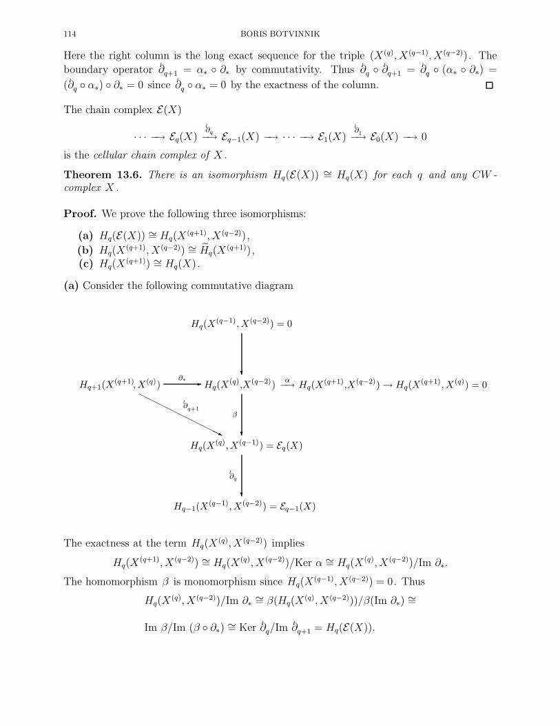
114 BORIS BOTVINNIK
Here the right column is the long exact sequence for the triple (X(q), X(q−1), X(q−2)). The
boundary operator ∂≀
q+1 = α∗ ∂∗ by commutativity. Thus ∂≀
q ∂≀
q+1 = ∂≀
q (α∗ ∂∗) =
(∂≀
q α∗) ∂∗ = 0 since ∂≀
q α∗ = 0 by the exactness of the column.
The chain complex E(X)
· · · −→ Eq(X)∂≀
q−→ Eq−1(X) −→ · · · −→ E1(X)∂≀
1−→ E0(X) −→ 0
is the cellular chain complex of X .
Theorem 13.6. There is an isomorphism Hq(E(X)) ∼= Hq(X) for each q and any CW -complex X .
Proof. We prove the following three isomorphisms:
(a) Hq(E(X)) ∼= Hq(X(q+1), X(q−2)),
(b) Hq(X(q+1), X(q−2)) ∼= Hq(X
(q+1)),(c) Hq(X
(q+1)) ∼= Hq(X).
(a) Consider the following commutative diagram
Hq(X(q−1),X(q−2)) = 0
?Hq+1(X
(q+1),X(q))HHHHHHHHHHj
∂≀
q+1
Hq(X(q),X(q−2))
?
β
α−→ Hq(X(q+1),X(q−2))→ Hq(X
(q+1),X(q)) = 0-∂∗
Hq(X(q),X(q−1)) = Eq(X)
?
∂≀
q
Hq−1(X(q−1),X(q−2)) = Eq−1(X)
The exactness at the term Hq(X(q), X(q−2)) implies
Hq(X(q+1), X(q−2)) ∼= Hq(X
(q), X(q−2))/Ker α ∼= Hq(X(q), X(q−2))/Im ∂∗.
The homomorphism β is monomorphism since Hq(X(q−1), X(q−2)) = 0. Thus
Hq(X(q), X(q−2))/Im ∂∗ ∼= β(Hq(X
(q), X(q−2)))/β(Im ∂∗) ∼=
Im β/Im (β ∂∗) ∼= Ker ∂≀
q/Im ∂≀
q+1 = Hq(E(X)).

NOTES ON THE COURSE “ALGEBRAIC TOPOLOGY” 115
(b) Consider long exact sequence for the triple (X(q+1), X(i), X(i−1)) where i = q − 2, q −3, . . . , 1, 0:
0=Hq(X(i), X(i−1))−→Hq(X
(q+1), X(i−1))∼=−→Hq(X
(q+1), X(i))−→Hq−1(X(i), X(i−1))= 0
Thus we obtain the isomorphisms:
Hq(X(q+1), X(q−2)) ∼= Hq(X
(q+1), X(q−3)) ∼= · · · ∼= Hq(X(q+1), X(0)) ∼= Hq(X
(q+1)).
(c) Consider long exact sequence in homology for the pair (X(j), X(q+1)) for j = q + 2,q + 3, . . .:
0 = Hq+1(X(j), X(q+1)) −→ Hq(X
(q+1))∼=−→ Hq(X
(j)) −→ Hq(X(j), X(q+1)) = 0.
Thus Hq(X(q+1)) ∼= Hq(X
(q+2)) ∼= · · · ∼= Hq(X).
13.5. Geometric meaning of the boundary homomorphism ∂≀
q . Consider closely the
groups Eq(X) and the boundary operator ∂≀
q : Eq(X) −→ Eq−1(X). First we recall that
Eq(X) =∑
i∈Eqλie
qi
where eqi are the q -th cells of the CW -complex X . The isomorphism of the group Eq(X)with free abelian group is not unique: it depends on the choice of the homeomorphismX(q)/X(q−1) ∼=
∨Sq . The choice of this homeomorphism is detemined by the characteris-
tic maps
DqX(q)-Φi
Sq−1
6
X(q−1)
6
-ϕi
The map of pairs (Φi, ϕi) : (Dq, Sq−1)→ (X(q), X(q−1)) induces the homeomorphism
Φi : Sq = Dq/Dq−1 −→ eq/∂eq ⊂ X(q)/X(q−1).
Definition 13.7. We say that two characteristic maps Φi,Φ′i : (Dq, Sq−1) −→ (X(q), X(q−1))
are of the same orientation if the composition (which is a homeomorphism)
SqΦi−→ eq/∂eq
(Φ′
i)−1
−−−−→ Sq
has degree one. It means that the map Φi (Φ′i)−1 is homotopic to the identity map. If
the degree of the map Φi (Φ′i)
−1 is −1, the characteristic maps Φi,Φ′i have the opposite
orientation.
Thus the group
Eq(X) =∑
i∈Eqλie
qi
should be thought as a free abelian group with oriented q -cells as generators.
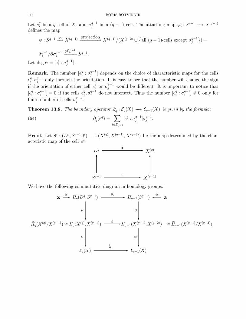
116 BORIS BOTVINNIK
Let eqi be a q -cell of X , and σq−1j be a (q− 1)-cell. The attaching map ϕi : Sq−1 −→ X(q−1)
defines the map
ψ : Sq−1 ϕi−→ X(q−1) projection−−−−−−−→ X(q−1)/(X(q−2) ∪all (q − 1)-cells except σq−1
j
) =
σq−1j /∂σq−1
j
(Φj)−1
−−−−→ Sq−1.
Let degψ = [eqi : σq−1j ].
Remark. The number [eqi : σq−1j ] depends on the choice of characteristic maps for the cells
eqi , σq−1j only through the orientation. It is easy to see that the number will change the sign
if the orientation of either cell eqi or σq−1j would be different. It is important to notice that
[eqi : σq−1j ] = 0 if the cells eqi , σ
q−1j do not intersect. Thus the number [eqi : σq−1
j ] 6= 0 only for
finite number of cells σq−1j .
Theorem 13.8. The boundary operator ∂≀
q : Eq(X) −→ Eq−1(X) is given by the formula:
(64) ∂≀
q(eq) =
∑
j∈Eq−1
[eq : σq−1j ]σq−1
j .
Proof. Let Φ : (Dq, Sq−1, ∅) −→ (X(q), X(q−1), X(q−2)) be the map determined by the char-acteristic map of the cell eq :
DqX(q)-Φ
Sq−1
6
X(q−1)
6
-ϕ
We have the following commutative diagram in homology groups:
Z Hq(Dq, Sq−1)
?
α
Hq−1(Sq−1)
?
β
Z-∼= -∂∗
∼=
Hq(X(q)/X(q−1)) ∼= Hq(X
(q),X(q−1))
?
∼=
Hq−1(X(q−1),X(q−2))
?
∼=
∼= Hq−1(X(q−1)/X(q−2))-∂
Eq(X) Eq−1(X)-∂≀
q

NOTES ON THE COURSE “ALGEBRAIC TOPOLOGY” 117
Here α and β are induced by the map Φ and α(1) = eq , β(1) = ∂≀
eq . Consider thecomposition
γ : Hq−1(Sq−1)
β−→ Hq−1(X(q−1), X(q−2)) = Hq−1(X
(q−1)/X(q−2)) = Hq−1(∨
j
Sq−1j )
=⊕
j
Hq−1(Sq−1j )
projection−−−−−−−→ Hq−1(Sq−1
σq−1j
).
By definition the degree of the homomorphism γ the coefficient with σq−1j in ∂
≀
eq is equal to
[eq : σq−1j ]. Thus
∂≀
q eq =
∑
j
[eq : σq−1j ]σq−1
j .
13.6. Some computations. First we compute again the homology groups Sn . We choosethe standard cell decomposition: Sn = en ∪ e0 .
n = 1. Here we have E0 = Z with the generator e0 , E1 = Z with the generator e1 , Eq = 0 ifq 6= 0, 1. Clearly ∂e1 = e0 − e0 = 0.
(1) n > 1. Here we have E0 = Z with the generator e0 , En = Z with the generator en ,
Eq = 0 if q 6= 0, n. Clearly ∂≀
qen = 0.
Thus in both cases we have that Hn(Sn) = Z, and Hq(S
n) = 0 if q 6= n.
13.7. Homology groups of RPn . Here we have to work a bit harder. We need the followinggeometric fact. Let the sphere Sn ⊂ Rn+1 is given by the equation x2
1 + · · ·+ x2n+1 = 1.
Lemma 13.9. Let A : Sn −→ Sn be the antipodal map, A : x 7→ −x, and ιn ∈ πn(Sn) be thegenerator represented by the identity map Sn −→ Sn . Then the homotopy class [A] ∈ πn(Sn)is equal to
[A] =
ιn, if n is odd,−ιn, if n is even.
Excercise 13.4. Prove Lemma 13.9.
Let e0, . . . , en be the cells in the standard cell decomposition of RPn . Recall that (RPn)(q) =RPq , and eq = RPq/RPq−1 , and that the Hopf map Sq−1 −→ RPq−1 is the attaching mapof the cell eq .
Lemma 13.10. Let e0, . . . , en be the cells in the standard cell decomposition of RPn . Then
[eq : eq−1] =
2 if q is odd,0, if q is even.
Proof. Let h : Sq−1 −→ RPq−1 be the Hopf map. We identify RPq−1 with the sphereSq−1 where the points x,−x ∈ Sq−1 are identified. The projective space RPq−2 ⊂ RPq−1 isthen the equator sphere Sq−2 ⊂ Sq−1 with the intipodal points identified as well. Now thecomposition
Sq−1 h−→ RPq−1 −→ RPq−1/RPq−2 = Sq−1
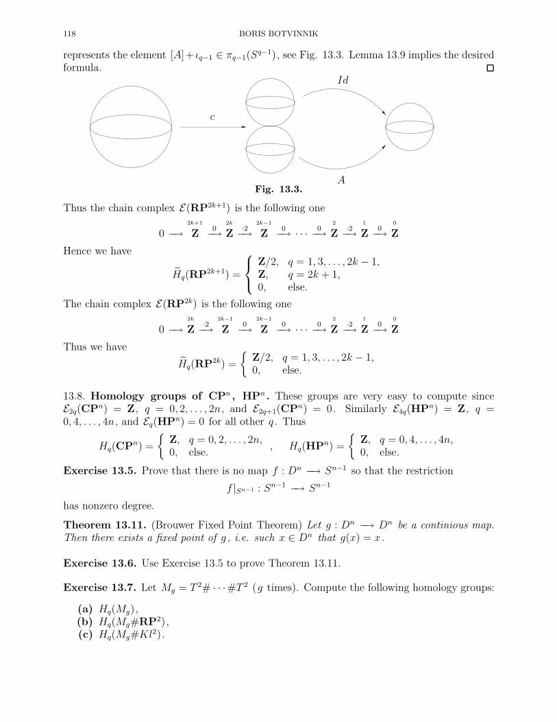
118 BORIS BOTVINNIK
represents the element [A]+ ιq−1 ∈ πq−1(Sq−1), see Fig. 13.3. Lemma 13.9 implies the desired
formula.
c
A
Id
Fig. 13.3.
Thus the chain complex E(RP2k+1) is the following one
0 −→2k+1
Z0−→
2k
Z·2−→
2k−1
Z0−→ · · · 0−→
2
Z·2−→
1
Z0−→
0
Z
Hence we have
Hq(RP2k+1) =
Z/2, q = 1, 3, . . . , 2k − 1,Z, q = 2k + 1,0, else.
The chain complex E(RP2k) is the following one
0 −→2k
Z·2−→
2k−1
Z0−→
2k−1
Z0−→ · · · 0−→
2
Z·2−→
1
Z0−→
0
Z
Thus we have
Hq(RP2k) =
Z/2, q = 1, 3, . . . , 2k − 1,0, else.
13.8. Homology groups of CPn , HPn . These groups are very easy to compute sinceE2q(CPn) = Z, q = 0, 2, . . . , 2n, and E2q+1(CPn) = 0. Similarly E4q(HPn) = Z, q =0, 4, . . . , 4n, and Eq(HPn) = 0 for all other q . Thus
Hq(CPn) =
Z, q = 0, 2, . . . , 2n,0, else.
, Hq(HPn) =
Z, q = 0, 4, . . . , 4n,0, else.
Exercise 13.5. Prove that there is no map f : Dn −→ Sn−1 so that the restriction
f |Sn−1 : Sn−1 −→ Sn−1
has nonzero degree.
Theorem 13.11. (Brouwer Fixed Point Theorem) Let g : Dn −→ Dn be a continious map.Then there exists a fixed point of g , i.e. such x ∈ Dn that g(x) = x.
Exercise 13.6. Use Exercise 13.5 to prove Theorem 13.11.
Exercise 13.7. Let Mg = T 2# · · ·#T 2 (g times). Compute the following homology groups:
(a) Hq(Mg),(b) Hq(Mg#RP2),(c) Hq(Mg#Kl
2).

NOTES ON THE COURSE “ALGEBRAIC TOPOLOGY” 119
Exercise 13.8. Let G(n, k) be the real Grassmannian manifold. Use the CW -decompositionof G(n, k) given in Section 4 to compute the homology groups:
(a) Hq(G(4, 2)),(b) Hq(G(5, 3)).
Exercise 13.9. Compute the homology groups:
(a) Hq(RP2 ×RP3),(b) Hq(RP5 ×RP3),(c) Hq(RP2 ×RP4).
Exercise 13.10. Let f(z) = anzn + an−1z
n−1 + · · ·+ a1z+ a0 be a complex polynomial withan 6= 0. Show that a polynomial f(z), viewed as a map f : C→ C, can be always extended
to a continious map f : S2 → S2 . Prove that the degree of the map f equals to n.
Exercise 13.11. Let f : S2n → S2n be a map. Prove that there exists a point x ∈ S2n suchthat either f(x) = x or f(x) = −x.
Exercise 13.12. Let f : Sn → Sn be a map of degree zero. Prove that there exist two pointsx, y ∈ Sn with f(x) = x and f(y) = −y .
Exercise 13.13. Construct a surjective map f : Sn → Sn of degree zero.
120 BORIS BOTVINNIK
14. Homology and homotopy groups
14.1. Homology groups and weak homotopy equivalence. Our goal here is to provethe following fact.
Theorem 14.1. Let f : X −→ Y be a weak homotopy equivalence. Then the inducedhomomorphism f∗ : Hq(X) −→ Hq(Y ) is an isomorphism for all q ≥ 0.
We start with a preliminary lemma.
Lemma 14.2. Let X be a topological space, α ∈ Hq(X). Then there exist a CW -complexK , a map f : K −→ X , an element β ∈ Hq(K) such that f∗(β) = α.
Proof. Let c =∑
i λifi , fi : ∆qi −→ X , be a chain representing α ∈ Hq(X). Consider the
space
K ′ =⊔
i
∆qi .
Recall that the simplex ∆q ⊂ Rq+1 is given by the vertices ∆q = (v0, . . . , vq), where v0 =(1, 0, . . . , 0), . . ., vq = (0, . . . , 0, 1). We can describe all subsimplices of ∆q as follows. Let0 ≤ t1 < · · · < tq−r ≤ q . Then
Γrt1,...,tq−r(∆q) = (v0, . . . , vt1 , . . . , vtq−r
, . . . , vq)
is an r -dimensional simplex with the vertices (v0, . . . , vt1 , . . . , vtq−r, . . . , vq). We introduce the
following equivalence relation in K :
Γrt1,...,tq−r(∆q
i ) ≡ Γrs1,...,sq−r(∆q
j) iff fi|Γrt1,...,tq−r
(∆qi ) = fj |Γr
s1,...,sq−r(∆q
j ).
Let K = K ′/ ∼. The maps fi : ∆qi −→ X determine a map f : K −→ X . Furthermore, let
gj : ∆qj
inclusion−−−−−−→ K ′ projection−−−−−−−→ K.
Then the chain c =∑
j λjgj ∈ Cq(K) maps to the chain c by construction. One has to notice
that c is a cycle since c is a cycle. Then β = [c] maps to α under the induced homomorphismf∗ .
There is the relative version of Lemma 14.2 which may be proved by slight modification ofthe above proof.
Lemma 14.3. Let (X,A) be a pair of topological spaces, α ∈ Hq(X,A). The there exista CW -pair (K,L), a map f : (K,L) −→ (X,A), and element β ∈ Hq(K,L), such thatf∗(β) = α.
Exercise 14.1. Prove Lemma 14.3.
Proof of Theorem 14.1. Recall that f : X −→ Y is a weak homotopy equivalence if forany CW -complex Z , the induced map f# : [Z,X] −→ [Z, Y ] is a bijection.
(1): f∗ is an epimorphism. Let α ∈ Hq(Y ). Then by Lemma 14.2 there exists a CW -complexK , a map g : K −→ Y such that g∗(β) = α . Consider a map h ∈ f−1
# ([g]) ∈ [K,X]. We
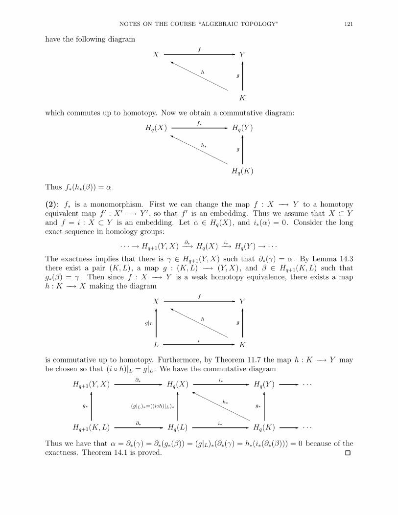
NOTES ON THE COURSE “ALGEBRAIC TOPOLOGY” 121
have the following diagram
X Y-f
K
HHHHHHHHHYh
6g
which commutes up to homotopy. Now we obtain a commutative diagram:
Hq(X) Hq(Y )-f∗
Hq(K)HHHHHHHHHY
h∗6
g
Thus f∗(h∗(β)) = α .
(2): f∗ is a monomorphism. First we can change the map f : X −→ Y to a homotopyequivalent map f ′ : X ′ −→ Y ′ , so that f ′ is an embedding. Thus we assume that X ⊂ Yand f = i : X ⊂ Y is an embedding. Let α ∈ Hq(X), and i∗(α) = 0. Consider the longexact sequence in homology groups:
· · · → Hq+1(Y,X)∂∗−→ Hq(X)
i∗−→ Hq(Y )→ · · ·The exactness implies that there is γ ∈ Hq+1(Y,X) such that ∂∗(γ) = α . By Lemma 14.3there exist a pair (K,L), a map g : (K,L) −→ (Y,X), and β ∈ Hq+1(K,L) such thatg∗(β) = γ . Then since f : X −→ Y is a weak homotopy equivalence, there exists a maph : K −→ X making the diagram
X Y-f
L
6g|L
K
HHHHHHHHHYh
6g
-i
is commutative up to homotopy. Furthermore, by Theorem 11.7 the map h : K −→ Y maybe chosen so that (i h)|L = g|L . We have the commutative diagram
Hq+1(Y,X) Hq(X) Hq(Y ) · · ·-∂∗ -i∗ -
Hq+1(K,L)
6g∗
Hq(L)
6(g|L)∗=((ih)|L)∗
Hq(K)HHHHHHHHHY
h∗6
g∗
· · ·-∂∗ -i∗ -
Thus we have that α = ∂∗(γ) = ∂∗(g∗(β)) = (g|L)∗(∂∗(γ) = h∗(i∗(∂∗(β))) = 0 because of theexactness. Theorem 14.1 is proved.

122 BORIS BOTVINNIK
Recall that we proved (Theorem 11.7) that a map f : X −→ Y is weak homotopy equivalenceif the induced homomorphism f∗ : πq(X, x0) −→ πq(Y, f(x0)) is an isomorphism for all q ≥ 0and x0 ∈ X . We reformulate Theorem 14.1:
Theorem 14.4. Let a map f : X −→ Y induce an isomorphism in homotopy groups f∗ :πq(X, x0) −→ πq(Y, f(x0)) for all q ≥ 0 and x0 ∈ X . Then f induces isomorphism in thehomology groups f∗ : Hq(X) −→ Hq(Y ) for all q ≥ 0 .
The following exercises show that some naive generalizations of Theorem 14.4 fail.
Exercise 14.2. Show that the spaces CP∞ × S3 and S2 have isomorphic homotopy groupsand different homology groups. Thus these spaces are not homotopy equivalent.
Exercise 14.3. Show that the spaces RPn × Sm and Sn ×RPm (n 6= m, m,n ≥ 2) haveisomorphic homotopy groups and different homology groups.
Exercise 14.4. Show that the spaces S1 ∨ S1 ∨ S2 and S1 × S1 have the same homologygroups and different homotopy groups.
Exercise 14.5. Show that the Hopf map h : S3 −→ S2 induces trivial homomorphism inreduced homology groups, and nontrivial homomorphism in homotopy groups.
Exercise 14.6. Show that the projection
S1 × S1 projection−−−−−−−→ (S1 × S1)/(S1 ∨ S1) = S2
induces trivial homomorphism in homotopy groups, and nontrivial homomorphism in homol-ogy groups.
14.2. Hurewicz homomorphism. Let X be a topological space with a base point x0 ∈ X .Let sn be a canonical generator of Hn(S
n), n = 1, 2, . . ., given by the homeomorphism
∂∆n+1∼=−→ Sn . For any element α ∈ πn(X, x0) consider a representative f : Sn −→ X ,
[f ] = α . We have the induced homomorphism f∗ : Hn(Sn) −→ Hn(X). Let
h(α) = f∗(sn) ∈ Hn(X).
Clearly the element h(α) ∈ Hn(X) does not depend on the choice of the representing mapf . Furthermore, the correspondence α 7→ h(α) determines the homomorphism
h : πn(X, x0) −→ Hn(X), n = 1, 2, . . . .
The homomorphism h is the Hurewicz homomorphism. The Hurewicz homomorphism isnatural with respect to maps (X, x0) −→ (Y, y0) of based spaces.
Exercise 14.7. Prove that h : πn(X, x0) −→ Hn(X) is a homomorphism.
Exercise 14.8. Let x0, x1 ∈ X , and γ : I −→ X be a path connecting the points x0, x1 :γ(0) = x0 , and γ(1) = x1 . The path γ determines the isomorphism
γ# : πn(X, x0) −→ πn(X, x1).

NOTES ON THE COURSE “ALGEBRAIC TOPOLOGY” 123
Prove that the following diagram commutes:
πn(X, x0)
@@
@@@R
h
πn(X, x1)
h
-γ#
Hn(X)
Theorem 14.5. (Hurewicz) Let (X, x0) be a based space, such that
(65) π0(X, x0) = 0, π1(X, x0) = 0, · · · , πn−1(X, x0) = 0,
where n ≥ 2. ThenH1(X) = 0, H2(X) = 0, · · · , Hn−1(X) = 0,
and the Hurewicz homomorphism h : πn(X, x0) −→ Hn(X) is an isomorphism.
Proof. By Theorem 11.10 there exist a CW -complex K and a weak homotopy equivalencef : K −→ X . Theorem 14.1 guarantees that f induces an isomorphism in homology groups.Thus it is enough to prove the statement in the case when X is a CW -complex. Then thecondition (65) means that X is (n−1)-connected CW -complex. Theorem 5.9 implies that upto homotopy equivalence X may be chosen so that it has a single zero-cell, and it does not haveany cells of dimensions 1, 2, . . . , n−1. In particular, this implies that H1(X) = 0, H2(X) = 0,· · · , Hn−1(X) = 0. Now the n-th skeleton of X is a wedge of spheres: X(n) =
∨i S
ni . Let
gi : Sni −→∨i S
ni be the embedding of the i-th sphere, and let rj : Sn −→ ∨
i Sni be the
attaching maps of the (n+1)-cells en+1j . The maps gi determine the generators of the group
πn(X(n)), and let ρj ∈ πn(X(n)) be the elements determined by the maps rj .
Theorem 11.6 describes the first nontrivial homotopy group πn(X, x0) as a factor-group ofthe homotopy group πn(X
(n)) ∼= Z⊕ · · · ⊕ Z by the subgroup generated by ρj . Notice thatthe cellular chain group
En(X) = Hn(X(n)) = Hn
(∨
i
Sni
),
and Hn(X) = En(X)/Im ∂≀
n+1 . Finally we notice that the Hurewicz homomorphism h :πn(S
n) −→ Hn(Sn) is an isomorphism. Thus we have the commutative diagram
πn
(∨
i
Sni
)Hn
(∨Sni
)-h
πn(Snj )
6(ρj)∗
Hn(Snj )
6(ρj)∗
-h
where the horizontal homomorphisms are isomorphisms. Hence h induces an isomorphismπn(X, x0) −→ Hn(X).
Corollary 14.6. Let X be a simply connected space, and H1(X) = 0, H2(X) = 0 · · ·Hn−1(X) = 0. Then π1(X) = 0, π2(X) = 0 · · · πn−1(X) = 0 and the Hurewicz homomor-phism h : πn(X, x0) −→ Hn(X) is an isomorphism.
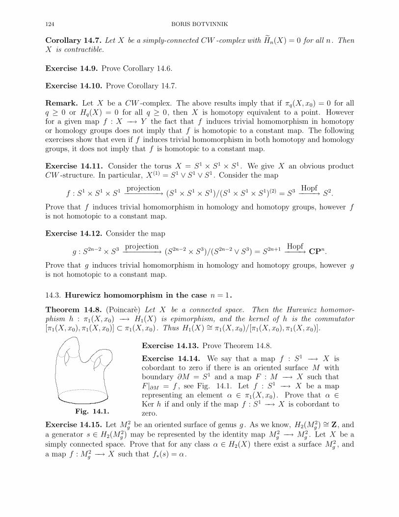
124 BORIS BOTVINNIK
Corollary 14.7. Let X be a simply-connected CW -complex with Hn(X) = 0 for all n. ThenX is contractible.
Exercise 14.9. Prove Corollary 14.6.
Exercise 14.10. Prove Corollary 14.7.
Remark. Let X be a CW -complex. The above results imply that if πq(X, x0) = 0 for allq ≥ 0 or Hq(X) = 0 for all q ≥ 0, then X is homotopy equivalent to a point. Howeverfor a given map f : X −→ Y the fact that f induces trivial homomorphism in homotopyor homology groups does not imply that f is homotopic to a constant map. The followingexercises show that even if f induces trivial homomorphism in both homotopy and homologygroups, it does not imply that f is homotopic to a constant map.
Exercise 14.11. Consider the torus X = S1 × S1 × S1 . We give X an obvious productCW -structure. In particular, X(1) = S1 ∨ S1 ∨ S1 . Consider the map
f : S1 × S1 × S1 projection−−−−−−−−→ (S1 × S1 × S1)/(S1 × S1 × S1)(2) = S3 Hopf−−−−→ S2.
Prove that f induces trivial homomorphism in homology and homotopy groups, however fis not homotopic to a constant map.
Exercise 14.12. Consider the map
g : S2n−2 × S3 projection−−−−−−−−→ (S2n−2 × S3)/(S2n−2 ∨ S3) = S2n+1 Hopf−−−−→ CPn.
Prove that g induces trivial homomorphism in homology and homotopy groups, however gis not homotopic to a constant map.
14.3. Hurewicz homomorphism in the case n = 1.
Theorem 14.8. (Poincare) Let X be a connected space. Then the Hurewicz homomor-phism h : π1(X, x0) −→ H1(X) is epimorphism, and the kernel of h is the commutator[π1(X, x0), π1(X, x0)] ⊂ π1(X, x0). Thus H1(X) ∼= π1(X, x0)/[π1(X, x0), π1(X, x0)].
Fig. 14.1.
Exercise 14.13. Prove Theorem 14.8.
Exercise 14.14. We say that a map f : S1 −→ X iscobordant to zero if there is an oriented surface M withboundary ∂M = S1 and a map F : M −→ X such thatF |∂M = f , see Fig. 14.1. Let f : S1 −→ X be a maprepresenting an element α ∈ π1(X, x0). Prove that α ∈Ker h if and only if the map f : S1 −→ X is cobordant tozero.
Exercise 14.15. Let M2g be an oriented surface of genus g . As we know, H2(M
2g )∼= Z, and
a generator s ∈ H2(M2g ) may be represented by the identity map M2
g −→ M2g . Let X be a
simply connected space. Prove that for any class α ∈ H2(X) there exist a surface M2g , and
a map f : M2g −→ X such that f∗(s) = α .
NOTES ON THE COURSE “ALGEBRAIC TOPOLOGY” 125
14.4. Relative version of the Hurewicz Theorem. One defines the relative Hurewiczhomomorphism h : πn(X,A, x0) −→ Hn(X,A) similarly to the regular Hurewicz homo-morphism. Let s ∈ Hn(D
n, Sn−1) be a canonical generator given by the homeomorphism
(∆n, ∂∆n)∼=−→ (Dn, Sn−1). Let f : (Dn, Sn−1) −→ (X,A) be a map representing an element
α ∈ πn(X.A). Then h(α) = f∗(sn) ∈ Hn(X,A). There is a relative version of the aboveHurewics Theorem:
Theorem 14.9. Let (X,A) be a pair of simply connected spaces, x0 ∈ A, such that
(66) π0(X,A, x0) = 0, π1(X,A, x0) = 0, · · · , πn−1(X,A, x0) = 0,
where n ≥ 2. Then
H1(X,A) = 0, H2(X,A) = 0, · · · , Hn−1(X,A) = 0,
and the Hurewicz homomorphism h : πn(X,A, x0) −→ Hn(X,A) is an isomorphism.
We do not give a proof of Theorem 14.9, however it is very similar to the proof of the aboveHurewicz Theorem.
Exercise 14.16. Prove Theorem 14.9.
Theorem 14.10. (Whitehead Theorem-II) Let X , Y be simply connected spaces andf : X −→ Y be a map.
(a) If the induced homomorphism in homotopy groups f∗ : πq(X, x0) −→ πq(Y, f(x0))is isomorphism for q = 2, 3, . . . , n − 1, and epimorphism if q = n, then thehomomorphism in homology groups f∗ : Hq(X) −→ Hq(Y ) is isomorphism forq = 2, 3, . . . , n− 1, and epimorphism if q = n.
(b) If the induced homomorphism in homology groups f∗ : Hq(X) −→ Hq(Y ) is isomor-phism for q = 2, 3, . . . , n− 1, and epimorphism if q = n, then the homomorphism inhomotopy groups f∗ : πq(X, x0) −→ πq(Y, f(x0)) is isomorphism for q = 2, 3, . . . , n−1,and epimorphism if q = n.
Proof. (a) We can assume that f : X −→ Y is an embedding, see Claim 9.1. Then the longexact sequence in homotopy
(67) · · · → πq(X, x0)f∗−→ πq(Y, x0) −→ πq(Y,X, x0)
∂−→ πq−1(X, x0)→ · · ·gives that if f∗ : πq(X, x0) −→ πq(Y, f(x0)) is isomorphism for q = 1, 2, 3, . . . , n − 1, andepimorphism if q = n, then πq(Y,X, x0) = 0 if q ≤ n. Then Theorem 14.9 implies thatHq(Y,X) = 0 for q ≤ n. Then the long exact sequence in homology
(68) · · · → Hq(X)f∗−→ Hq(Y ) −→ Hq(Y,X) −→ Hq−1(X)→ · · ·
implies that f∗ : Hq(X)→ Hq(Y ) is isomorphism for q = 1, 2, 3, . . . , n− 1, and epimorphismif q = n.
(b) Analogously, let f∗ : Hq(X) → Hq(Y ) be an isomorphism for q = 1, 2, 3, . . . , n − 1,and epimorphism if q = n. Then the long exact sequence in homology (68) implies thatHq(Y,X, x0) = 0 for q ≤ n. Then again, Theorem 14.9 implies that πq(Y,X, x0) = 0 forq ≤ n and the exact sequence (67) gives that f∗ : πq(X, x0) −→ πq(Y, f(x0)) is isomorphism
126 BORIS BOTVINNIK
for q = 1, 2, 3, . . . , n−1, and epimorphism if q = n. Thus in both cases the relative HurewiczTheorem 14.9 implies the desired result.
Corollary 14.11. Let X , Y be simply connected spaces and f : X −→ Y be a map whichinduces isomorphism f∗ : Hq(X) −→ Hq(Y ) for all q ≥ 0. Then f is weak homotopyequivalence. (In particular, if X , Y are CW -complexes, then f is homotopy equivalence.)
Exercise 14.17. Let X be a connected, simply connected CW -complex with Hn(X) = Z,
n ≥ 2, and Hq(X) = 0 if q 6= n. Prove that X is homotopy equivalent to Sn .
NOTES ON THE COURSE “ALGEBRAIC TOPOLOGY” 127
15. Homology with coefficients and cohomology groups
Here we define homology and cohomology groups with coefficients in arbitrary abelian groupG. We should be aware that these constructions could be done rather formally by means ofbasic homological algebra. We choose to avoid a total “algebraization” of those constructions:there are great classical books (say, by S. MacLane, Homology, Springer, 1967 or by S.Eilenberg & N. Steenrod, Foundations of Algebraic Topology) where you can find the mostabstract algebraic approach concerning the homology and cohomology theories. We willdescribe only those algebraic constructions which are really necessary.
15.1. Definitions. Let G be an abelian group. A singular q -chain of a space X with coef-ficients in G is a linear combination
∑
i
λifi, where λi ∈ G, and fi : ∆q −→ X is a singular simplex.
We denote a group of q -chains Cq(X;G). Clearly, Cq(X;G) = Cq(X) ⊗ G. The bound-ary operator ∂q : Cq(X;G) −→ Cq−1(X;G) is induced by the regular boundary operator∂q : Cq(X) −→ Cq(X). In more detail, recall that a simplex ∆q is defined by the vertices(v0, . . . , vq), and Γj∆
q is the face of ∆q given by the vertices (v0, . . . , vj, . . . , vq). Then
∂q(f : ∆q −→ X) =
q∑
j=0
(−1)j(f |Γj∆q : Γj∆q −→ X).
Let C∗(X) be the singular chain complex:
(69) · · · ∂q+1−−−→ Cq(X)∂q−→ Cq−1(X)
∂q−1−−−→ · · · ∂2−→ C1(X)∂1−→ C0(X) −→ 0.
Then we have the chain complex C∗(X)⊗G:
· · · ∂q+1−−−→ Cq(X)⊗G ∂q−→ Cq−1(X)⊗G ∂q−1−−−→ · · · ∂2−→ C1(X)⊗G ∂1−→ C0(X)⊗G −→ 0.
We define the homology groups with coefficients in G:
Hq(X;G) = Hq(C∗(X)⊗G) =Ker(∂q : Cq(X)⊗G −→ Cq−1(X)⊗G)
Im(∂q+1 : Cq+1(X)⊗G −→ Cq(X)⊗G).
Now we consider the cochain complex C∗(X;G) = Hom(C∗(X), G):
· · · δq
←− Hom(Cq(X), G)δq−1
←−−− Hom(Cq−1(X), G)δq−2
←−−− · · · δ0←− Hom(C0(X), G) ←− 0.
In other words, a cochain ξ ∈ Hom(Cq(X), G) = Cq(X;G) is a linear function on Cq(X)with values in the group G, ξ : Cq(X)→ G.
It is convenient to denote ξ(c) = 〈ξ, c〉 ∈ G. Notice that by definition, 〈δqξ, a〉 = 〈ξ, ∂q+1a〉 ,where ξ ∈ Cq(X;G), and a ∈ Cq+1(X). Clearly δq+1δq = 0 since
〈δq+1δqξ, a〉 = 〈δqξ, ∂q+2a〉 = 〈ξ, ∂q+1∂q+2a〉 = 0.
We define the cohomology groups
Hq(X;G) = Hq(C∗(X;G)) =Ker(δq : Cq(X;G) −→ Cq+1(X;G))
Im(δq−1 : Cq−1(X;G) −→ Cq(X;G)).
128 BORIS BOTVINNIK
Recall that there is a canonical homomorphism ǫ : C0(X) −→ Z sending c =∑
j λjfj to the
sum∑
j λj ∈ Z. The homomorphism ǫ induces the homomorphisms
ǫ∗ : C0(X;G) −→ G and ǫ∗ : G −→ C0(X;G).
Clearly ǫ∗ :∑
j λjfj 7→∑
j λj ∈ G, and ǫ∗ : λ 7→ ξλ , where 〈ξλ, fj〉 = λ for any generator
fj ∈ C0(X). Then we define the complexes C∗(X)⊗G and C∗(X;G) as
· · · ∂q+1−−→ Cq(X)⊗G ∂q−→ Cq−1(X)⊗G ∂q−1−−→ · · · ∂1−→ C0(X)⊗G ǫ∗−→ G −→ 0,
· · · δq
←− Cq(X;G)δq−1
←−− Cq−1(X;G)δq−2
←−− · · · δ0←− C0(X;G)ǫ∗←− G←− 0.
Thus H0(X;G) = Ker ǫ∗/Im ∂1 , and H0(X;G) = Ker δ0/Im ǫ∗ . It is convenient to call theelements of Cq(X;G) a cochain, the elements of Zq(X;G) = Ker δq ⊂ Cq(X;G) cocycles,and the elements of Bq(X;G) = Im δq−1 ⊂ Zq(X;G) coboundaries.
15.2. Basic propertries of H∗(−;G) and H∗(−;G). Here we list those properties of homol-ogy and cohomology groups which are parallel to the above features of the integral homologygroups.
(1) (Naturality) The homology groups Hq(X;G) and cohomology groups Hq(X;G) arenatural, i.e. if f : X −→ Y is a map, then it induces the homomorphisms
f∗ : Hq(X;G) −→ Hq(Y ;G), and f ∗ : Hq(Y ;G) −→ Hq(X;G).
In other words, the homology H∗(−;G) is a covariant functor on the category ofspaces, and the cohomology H∗(−;G) is a contravariant functor.
(2) (Homotopy invariance) Let f ∼ g : X −→ Y . then
f∗ = g∗ : Hq(X;G) −→ Hq(Y ;G), and f ∗ = g∗ : Hq(Y ;G) −→ Hq(X;G).
(3) (Additivity) Let X =⊔j Xj be a disjoint union. Then
H∗
(⊔
j
Xj;G
)∼=⊕
j
H∗(Xj;G), and H∗
(⊔
j
Xj;G
)∼=∏
j
H∗(Xj ;G).
(4) (Homology of the point) H0(pt;G) = G, Hq(pt;G) = 0, and Hq(pt;G) = 0,Hq(pt;G) = 0 for q ≥ 1.
(5) (Long exact sequences) For any pair (X,A) there are the following long exact se-quences:
· · · → Hq(A;G) −→ Hq(X;G) −→ Hq(X,A;G)∂−→ Hq−1(A;G)→ · · · ,
· · · → Hq(X,A;G) −→ Hq(X;G) −→ Hq(A;G)δ−→ Hq+1(X,A;G)→ · · ·
(6) (Excision) If (X,A) is a Borsuk pair, then
Hq(X,A;G) ∼= Hq(X/A;G), Hq(X,A;G) ∼= Hq(X/A;G).
In general case, there are the excision isomorphisms:
Hq(X \B,A \B) ∼= Hq(X,B), Hq(X \B,A \B) ∼= Hq(X,B),
under the same assumptions as before (i.e. that B ⊂ A and B ⊂o
A).
NOTES ON THE COURSE “ALGEBRAIC TOPOLOGY” 129
(7) (Mayer-Vietoris long exact sequnces) Let X1, X2 ⊂ X , and X1∪X2 = X ,o
X1∪o
X2 =X . Then there are the Mayer-Vietoris long exact sequnces:
· · · → Hq(X1 ∩X2;G)α∗−→ Hq(X1;G)⊕Hq(X2;G)
β∗−→ Hq(X1 ∪X2;G)∂−→ · · ·
· · · → Hq(X1 ∪X2;G)α∗
−→ Hq(X1;G)⊕Hq(X2;G)β∗
−→ Hq(X1 ∩X2;G)δ−→ · · ·
Exercise 15.1. Compute the groups Hq(Sn;G) and Hq(Sn;G).
Exercise 15.2. Compute the groups Hq(CPn;G) and Hq(CPn;G).
Exercise 15.3. Compute the groups Hq(RPn;Z/p), Hq(RPn;Z/p) for any prime p.
Exercise 15.4. Let Mg be an oriented surface of genus g . Compute the groups Hq(Mg;Z/p)and Hq(Mg;Z/p) for any prime p.
Exercise 15.5. Compute the homology and cohomology groups Hq(Mg#RP2;Z/p) andHq(Mg#RP2;Z/p) for any prime p.
Exercise 15.6. Compute the homology and cohomology groups Hq(Mg#Kl2;Z/p) and
Hq(Mg#Kl2;Z/p) for any prime p.
15.3. Coefficient sequences. We have to figure out the relationship between homology andcohomology groups with different coefficients. Let ϕ : G −→ H be a homomorphism ofabelian groups. Then clearly ϕ induces the chain (cochain) maps of complexes:
ϕ# : C∗(X;G) −→ C∗(X;H), and ϕ# : C∗(X;G) −→ C∗(X;H).
(Notice that the homomorphisms ϕ# and ϕ# are going in the same direction.) Thus ϕinduces the homomorphisms:
ϕ∗ : H∗(X;G) −→ H∗(X;H) and ϕ∗ : H∗(X;G) −→ H∗(X;H).
Now let 0 −→ G′ α−→ Gβ−→ G′′ −→ 0 be a short exact sequence of abelian groups. It is easy
to notice that this short exact sequnce induces the short exact sequnces of complexes:
0 −→ C∗(X;G′)α#−→ C∗(X;G)
β#−→ C∗(X;G′′) −→ 0,
0 −→ C∗(X;G′)α#
−→ C∗(X;G)β#
−→ C∗(X;G′′) −→ 0.
These short exact sequences immediately imply the coefficient exact sequences:
· · · → Hq(X;G′)α∗−→ Hq(X;G)
β∗−→ Hq(X;G′′)∂−→ Hq−1(X;G′)→ · · · ,
· · · → Hq(X;G′)α∗
−→ Hq(X;G)β∗
−→ Hq(X;G′′)δ−→ Hq+1(X;G′)→ · · · ,
Example. Consider the short exact sequence 0 −→ Z·m−→ Z −→ Z/m −→ 0. Then we have
the connecting homomorphisms
∂ = βm : Hq(X;Z/m) −→ Hq+1(X;Z), and δ = βm : Hq(X;Z/m) −→ Hq+1(X;Z).

130 BORIS BOTVINNIK
These homomorphisms are known as the Bockstein homomorphisms. Let α ∈ Hq(X;Z/m),and a ∈ Cq(X;Z/m) a cycle representing α . Then ∂q(a) = 0 in Cq−1(X;Z/m), however ingeneral, ∂q(a) 6= 0 in Cq−1(X;Z). It is easy to check that ∂q(a) = m·b, where b ∈ Cq−1(X;Z)
is a cycle. Thus βm(α) =[∂q(a)m
]∈ Hq−1(X;Z).
15.4. The universal coefficient Theorem for homology groups. We recall few basicconstructions from elementary group theory. Let G be an abelian group. Then there is a freeresolution of G:
0 −→ Rβ−→ F
α−→ G −→ 0,
i.e. the above sequence is exact and the groups F , R are free abelian. Roughly a choice offree resolution corresponds to a choice of generators and relations for the abelian group G.
This choice is not unique, however, if 0 −→ R1β1−→ F1
α1−→ G −→ 0 is another free resolution,there exist homomorphisms ψ : F −→ F1 , θ : R −→ R1 which make the following diagramcommute:
0 R
?
θ
F
?
ψ
G
?
Id
0- -β -α -
0 R1 F1 G 0- -β1 -α1 -
Now let H be an abelian group.
Claim 15.1. There is the exact sequence
0 −→ Ker(β ⊗ 1) −→ R⊗H β⊗1−−→ F ⊗H α⊗1−−→ G⊗H −→ 0.
Exercise 15.7. Prove Claim 15.1.
We define Tor(G,H) = Ker(β ⊗ 1).
Exercise 15.8. Prove that the group Tor(G,H) is well-defined, i.e. it does not depend onthe choice of resolution.
Let 0 −→ Rβ−→ F
α−→ G −→ 0 be a resolution of G. We denote R(G) the chain complex
0 −→ Rβ−→ F −→ 0.
Clearly H0(R(G)) = G, and Hj(R(G)) = 0 if j > 0. Consider the complex R(G)⊗H :
0 −→ R⊗H β−→ F ⊗H −→ 0.
By definition we have that
Hj(R(G)⊗H) =
G⊗H if j = 0,Tor(G,H) if j = 1,
0 else.
Now consider an exact sequence
(70) 0 −→ G′ −→ G −→ G′′ −→ 0.

NOTES ON THE COURSE “ALGEBRAIC TOPOLOGY” 131
The sequence (70) induces a short exact sequence of the complexes:
0 −→ R(G′) −→ R(G) −→ R(G′′) −→ 0,
and a short exact sequence of the complexes:
0 −→ R(G′)⊗H −→ R(G)⊗H −→ R(G′′)⊗H −→ 0.
Thus we have the long exact sequence in homology groups:
(71) 0→ Tor(G′, H)→ Tor(G,H)→ Tor(G′′, H)→ G′ ⊗H → G⊗H → G′′ ⊗H → 0
Exercise 15.9. Let G,H be abelian groups. Prove that there is a canonical isomorphismTor(G,H) ∼= Tor(H,G).
Exercise 15.10. Let G,G′, G′′ be abelian groups. Prove the isomorphism
Tor(Tor(G,G′), G′′) ∼= Tor(G,Tor(G′, G′′)).
Exercise 15.11. Let F be a free abelian group. Show that Tor(F,G) = 0 for any abeliangroup G.
Exercise 15.12. Let G be an abelian group. Denote T (G) a maximal torsion subgroup ofG. Show that Tor(G,H) ∼= T (G)⊗ T (H) for finite generated abelian groups G,H . Give anexample of abelian groups G,H , so that Tor(G,H) 6= T (G)⊗ T (H).
Theorem 15.1. Let X be a space, G be an abelian group. Then there is a split short exactsequence
(72) 0→ Hq(X)⊗G −→ Hq(X;G) −→ Tor(Hq−1(X), G)→ 0
Remark. The splitting of the sequence (15.1) is not natural. In the course of the proof weshall see that that this splitting depends on a splitting of the chain complex C∗(X).
Proof. Let 0 −→ Rβ−→ F
α−→ G −→ 0 be a free resolution of G. We have the five-termexact sequence
Hq(X;R)β∗−→ Hq(X;F )
α∗−→ Hq(X;G)∂−→ Hq−1(X;R)
β∗−→ Hq−1(X;F ).
We notice that Hq(X;R) ∼= Hq(X) ⊗ R , and Hq(X;F ) ∼= Hq(X) ⊗ F . Thus we have theexact sequence
(73) Hq(X)⊗ R β∗−→ Hq(X)⊗ F α∗−→ Hq(X;G)∂−→ Hq−1(X)⊗ R β∗−→ Hq−1(X)⊗ F
Consider carefully the sequence (73). First, we notice that it gives a short exact sequence
0 −→ Coker β∗ −→ Hq(X;G) −→ Ker β∗ −→ 0,
where
Coker β∗ = (Hq(X)⊗ F )/Im(β∗ : Hq(X)⊗R β∗−→ Hq(X)⊗ F ) and
Ker β∗ = Ker(β∗ : Hq−1(X)⊗R β∗−→ Hq−1(X)⊗ F ).
On the other hand, β∗ = 1 ⊗ β = β ⊗ 1. Hence Coker β∗ = Hq(X) ⊗ G, and Ker β∗ =Tor(Hq−1(X), G).
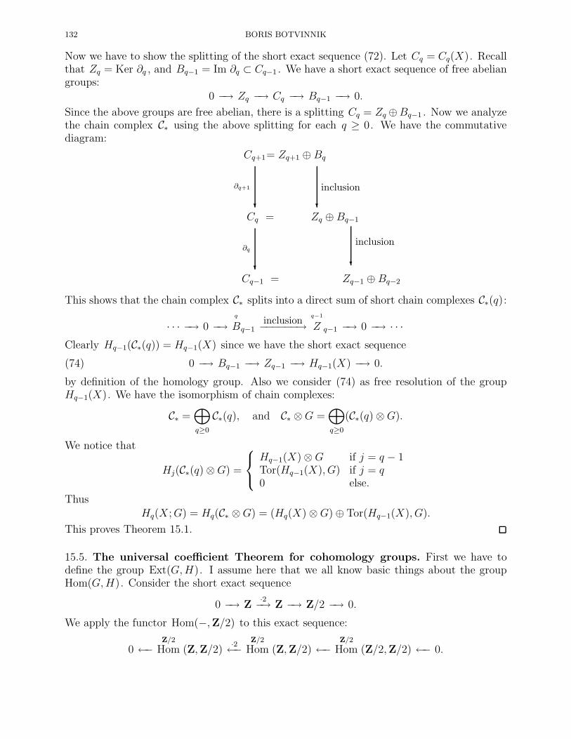
132 BORIS BOTVINNIK
Now we have to show the splitting of the short exact sequence (72). Let Cq = Cq(X). Recallthat Zq = Ker ∂q , and Bq−1 = Im ∂q ⊂ Cq−1 . We have a short exact sequence of free abeliangroups:
0 −→ Zq −→ Cq −→ Bq−1 −→ 0.
Since the above groups are free abelian, there is a splitting Cq = Zq ⊕Bq−1 . Now we analyzethe chain complex C∗ using the above splitting for each q ≥ 0. We have the commutativediagram:
?
inclusion
Cq+1
?
∂q+1
= Zq+1 ⊕ Bq
?
inclusion
Cq =
?
∂q
Zq ⊕ Bq−1
Cq−1 = Zq−1 ⊕ Bq−2
This shows that the chain complex C∗ splits into a direct sum of short chain complexes C∗(q):
· · · −→ 0 −→q
Bq−1inclusion−−−−−−→
q−1
Z q−1 −→ 0 −→ · · ·Clearly Hq−1(C∗(q)) = Hq−1(X) since we have the short exact sequence
(74) 0 −→ Bq−1 −→ Zq−1 −→ Hq−1(X) −→ 0.
by definition of the homology group. Also we consider (74) as free resolution of the groupHq−1(X). We have the isomorphism of chain complexes:
C∗ =⊕
q≥0
C∗(q), and C∗ ⊗G =⊕
q≥0
(C∗(q)⊗G).
We notice that
Hj(C∗(q)⊗G) =
Hq−1(X)⊗G if j = q − 1Tor(Hq−1(X), G) if j = q0 else.
ThusHq(X;G) = Hq(C∗ ⊗G) = (Hq(X)⊗G)⊕ Tor(Hq−1(X), G).
This proves Theorem 15.1.
15.5. The universal coefficient Theorem for cohomology groups. First we have todefine the group Ext(G,H). I assume here that we all know basic things about the groupHom(G,H). Consider the short exact sequence
0 −→ Z·2−→ Z −→ Z/2 −→ 0.
We apply the functor Hom(−,Z/2) to this exact sequence:
0 ←−Z/2
Hom (Z,Z/2)·2←−
Z/2
Hom (Z,Z/2) ←−Z/2
Hom (Z/2,Z/2) ←− 0.
NOTES ON THE COURSE “ALGEBRAIC TOPOLOGY” 133
Clearly this sequence is not exact.
Let G be an abelian group and 0 −→ Rβ−→ F
α−→ G −→ 0 be a free resolution.
Claim 15.2. Let H be an abelian group. The following sequence is exact:
(75) 0 ←− Coker β# ←− Hom(R,H)β#
←−− Hom(F,H)α#
←−− Hom(G,H) ←− 0.
Exercise 15.13. Prove Claim 15.2.
We define Ext(G,H) = Coker β# . Consider the cochain complex Hom(R(G), H):
0 ←− Hom(R,H)β#
←−− Hom(F,H) ←− 0.
Then Claim 15.2 implies that
Hj(Hom(R(G), H)) =
Hom(G,H) if j = 0,Ext(G,H) if j = 1,0 else.
Exercise 15.14. Prove that the group Ext(G,H) is well defined, i.e. it does not depend onthe choice of free resolution of G.
Exercise 15.15. Let 0 −→ G′ −→ G −→ G′′ −→ 0 be a short exact sequence of abeliangroups. Prove that it induces the following exact sequence:
0→ Hom(G′′, H)→ Hom(G,H)→ Hom(G′, H)→
Ext(G′′, H)→ Ext(G,H)→ Ext(G′, H)→ 0
Exercise 15.16. Prove that Ext(Z, H) = 0 for any group H .
Exercise 15.17. Prove the isomorphisms: Ext(Z/m,Z/n) ∼= Z/m ⊗ Z/n, Ext(Z/m,Z) ∼=Z/m.
Exercise 15.18. Let G or H be Q, R or C. Then Ext(G,H) = 0.
Theorem 15.2. Let X be a space, G an abelian group. Then there is a split exact sequence
(76) 0 −→ Ext(Hq−1(X), G) −→ Hq(X;G) −→ Hom(Hq(X), G) −→ 0
for each q ≥ 0. Again, the splitting of this sequence is not natural.
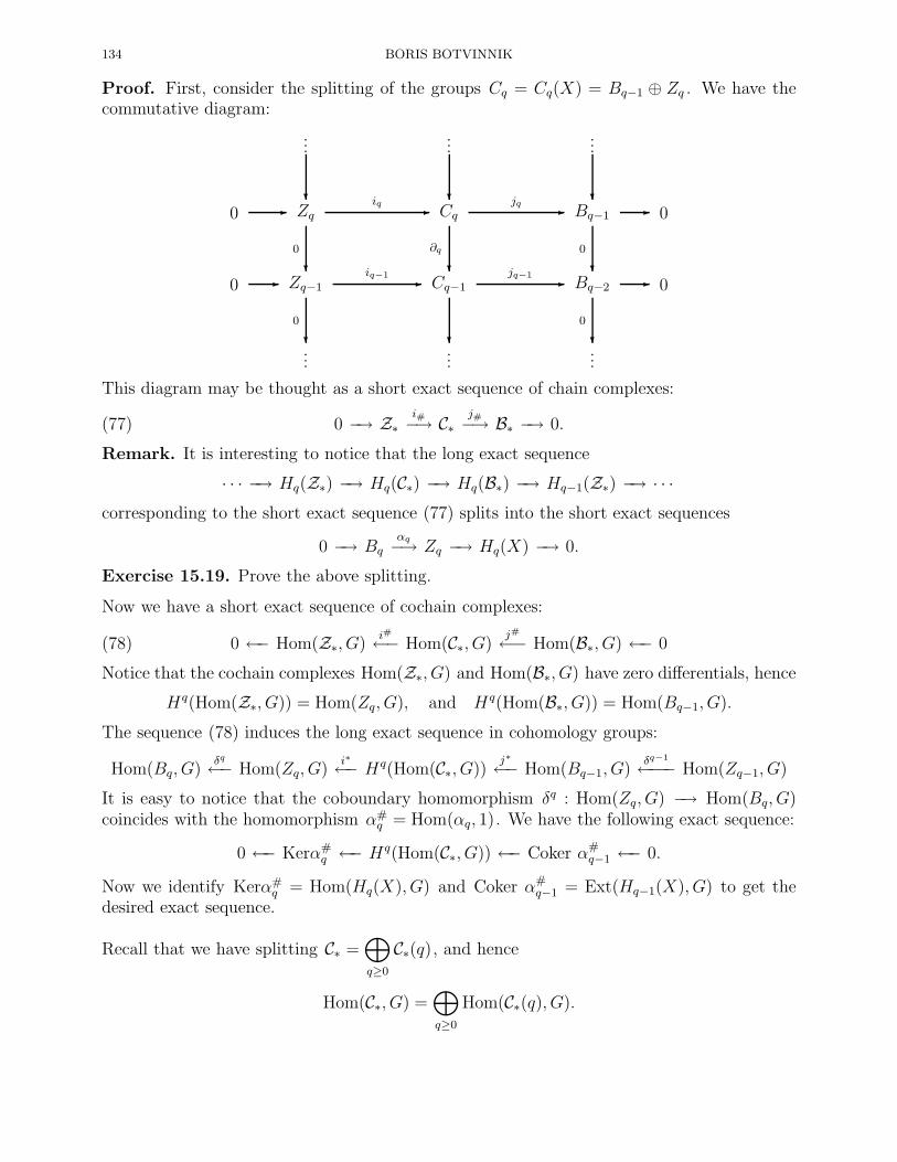
134 BORIS BOTVINNIK
Proof. First, consider the splitting of the groups Cq = Cq(X) = Bq−1 ⊕ Zq . We have thecommutative diagram:
...
?
...
?
...
?0 Zq
?0
Cq
?∂q
Bq−1
?0
0- -iq -jq -
0 Zq−1
?0
Cq−1
?
Bq−2
?0
0- -iq−1 -
jq−1 -
......
...
This diagram may be thought as a short exact sequence of chain complexes:
(77) 0 −→ Z∗i#−→ C∗
j#−→ B∗ −→ 0.
Remark. It is interesting to notice that the long exact sequence
· · · −→ Hq(Z∗) −→ Hq(C∗) −→ Hq(B∗) −→ Hq−1(Z∗) −→ · · ·corresponding to the short exact sequence (77) splits into the short exact sequences
0 −→ Bqαq−→ Zq −→ Hq(X) −→ 0.
Exercise 15.19. Prove the above splitting.
Now we have a short exact sequence of cochain complexes:
(78) 0 ←− Hom(Z∗, G)i#←− Hom(C∗, G)
j#←− Hom(B∗, G) ←− 0
Notice that the cochain complexes Hom(Z∗, G) and Hom(B∗, G) have zero differentials, hence
Hq(Hom(Z∗, G)) = Hom(Zq, G), and Hq(Hom(B∗, G)) = Hom(Bq−1, G).
The sequence (78) induces the long exact sequence in cohomology groups:
Hom(Bq, G)δq
←− Hom(Zq, G)i∗←− Hq(Hom(C∗, G))
j∗←− Hom(Bq−1, G)δq−1
←−−− Hom(Zq−1, G)
It is easy to notice that the coboundary homomorphism δq : Hom(Zq, G) −→ Hom(Bq, G)coincides with the homomorphism α#
q = Hom(αq, 1). We have the following exact sequence:
0 ←− Kerα#q ←− Hq(Hom(C∗, G)) ←− Coker α#
q−1 ←− 0.
Now we identify Kerα#q = Hom(Hq(X), G) and Coker α#
q−1 = Ext(Hq−1(X), G) to get thedesired exact sequence.
Recall that we have splitting C∗ =⊕
q≥0
C∗(q), and hence
Hom(C∗, G) =⊕
q≥0
Hom(C∗(q), G).

NOTES ON THE COURSE “ALGEBRAIC TOPOLOGY” 135
Consider the cochain complex Hom(C∗(q), G):
0 ←−q
Hom (Bq−1, G) ←−q−1
Hom (Zq−1, G) ←− 0.
We notice that the sequence 0 −→ Bq−1 −→ Zq−1 −→ Hq−1(X) −→ 0 may be considered asfree resolution of the group Hq−1(X). Thus we have:
Hj(Hom(C∗(q), G)) =
Hom(Hq−1(X), G) if j = q − 1,Ext(Hq−1(X), G) if j = q,0 else.
Thus we use the above splitting of Hom(C∗, G) to get the isomorphism:
Hq(X;G) = Hq(Hom(C∗, G)) = Hom(Hq(X), G)⊕ Ext(Hq−1(X), G).
This completes the proof of Theorem 15.2.
Theorem 15.3. Let X be a space, and G an abelian group. Then there is a split exactsequence
0 −→ Hq(X;Z)⊗G −→ Hq(X;G) −→ Tor(Hq+1(X;Z), G) −→ 0
for any q ≥ 0. Again the splitting is not natural.
Exercise 15.20. Prove Theorem 15.3.
Let G be a finitely generated abelian group. It is convenient to denote F (G) the maximumfree abelian subgroup of G, and T (G) the maximum torsion subgroup, so that G = F (G)⊕T (G). Perhaps such decomposition makes only for finitely generated groups.
Exercise 15.21. Let X be a space so that the groups Hq(X) are finitely generated. Provethat Hq(X;Z) are also finitely generated and Hq(X;Z) ∼= F (Hq(X;Z))⊕ T (Hq−1(X;Z)).
Exercise 15.22. Let F be Q, R or C. Prove that
Hq(X;F ) = Hq(X)⊗ F, Hq(X;F ) = Hom(Hq(X), F ).
Exercise 15.23. Let F be a free abelian group. Show that Ext(G,F ) = 0 for any abeliangroup G.
Exercise 15.23. Let X be a finite CW -complex, and F be a field. Prove that the number
χ(X)F =∑
q≥0
(−1)q dim Hq(X;F)
does not depend on the field F and is equal to the Euler characteristic
χ(X) =∑
q≥0
(−1)q # of q -cells of X .
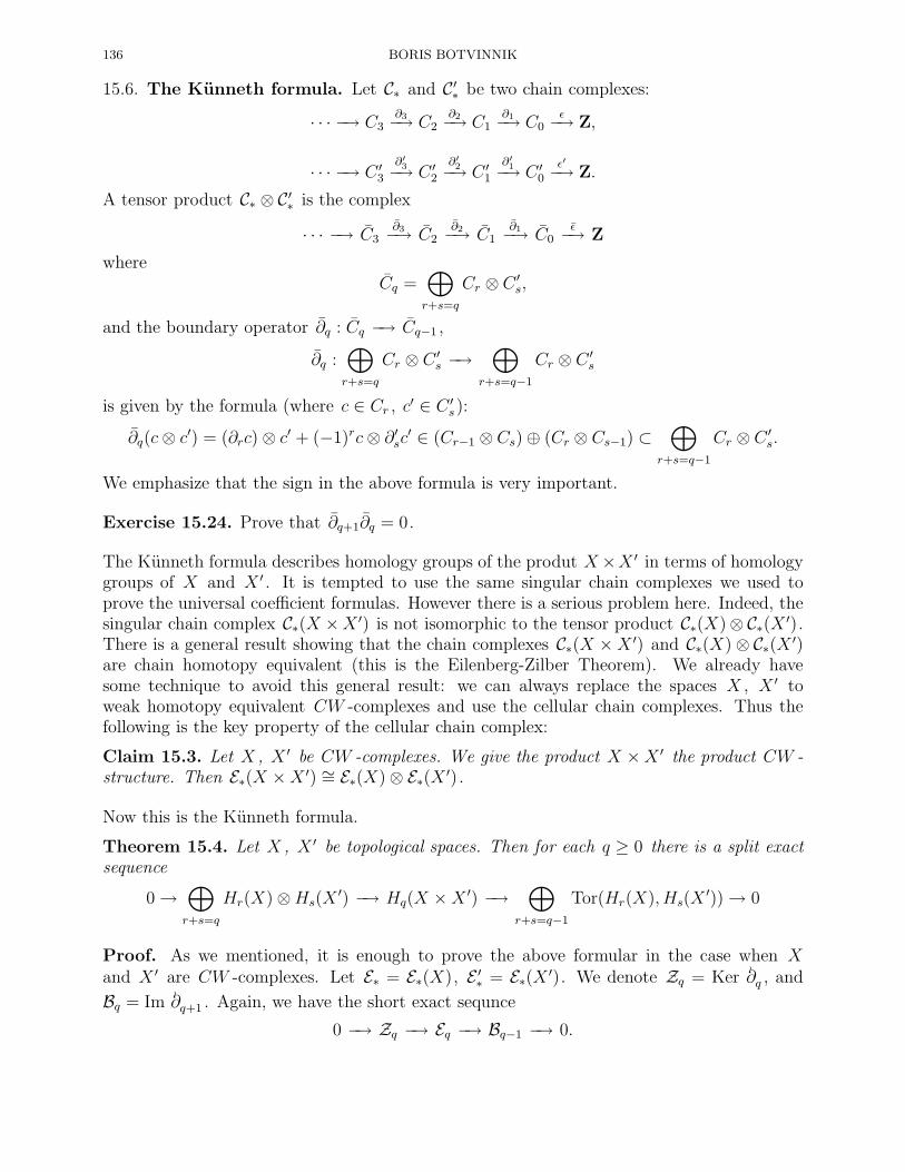
136 BORIS BOTVINNIK
15.6. The Kunneth formula. Let C∗ and C′∗ be two chain complexes:
· · · −→ C3∂3−→ C2
∂2−→ C1∂1−→ C0
ǫ−→ Z,
· · · −→ C ′3
∂′3−→ C ′2
∂′2−→ C ′1
∂′1−→ C ′0
ǫ′−→ Z.
A tensor product C∗ ⊗ C′∗ is the complex
· · · −→ C3∂3−→ C2
∂2−→ C1∂1−→ C0
ǫ−→ Z
whereCq =
⊕
r+s=q
Cr ⊗ C ′s,
and the boundary operator ∂q : Cq −→ Cq−1 ,
∂q :⊕
r+s=q
Cr ⊗ C ′s −→
⊕
r+s=q−1
Cr ⊗ C ′s
is given by the formula (where c ∈ Cr , c′ ∈ C ′s ):
∂q(c⊗ c′) = (∂rc)⊗ c′ + (−1)rc⊗ ∂′sc′ ∈ (Cr−1 ⊗ Cs)⊕ (Cr ⊗ Cs−1) ⊂⊕
r+s=q−1
Cr ⊗ C ′s.
We emphasize that the sign in the above formula is very important.
Exercise 15.24. Prove that ∂q+1∂q = 0.
The Kunneth formula describes homology groups of the produt X×X ′ in terms of homologygroups of X and X ′ . It is tempted to use the same singular chain complexes we used toprove the universal coefficient formulas. However there is a serious problem here. Indeed, thesingular chain complex C∗(X ×X ′) is not isomorphic to the tensor product C∗(X)⊗ C∗(X ′).There is a general result showing that the chain complexes C∗(X ×X ′) and C∗(X)⊗ C∗(X ′)are chain homotopy equivalent (this is the Eilenberg-Zilber Theorem). We already havesome technique to avoid this general result: we can always replace the spaces X , X ′ toweak homotopy equivalent CW -complexes and use the cellular chain complexes. Thus thefollowing is the key property of the cellular chain complex:
Claim 15.3. Let X , X ′ be CW -complexes. We give the product X ×X ′ the product CW -structure. Then E∗(X ×X ′) ∼= E∗(X)⊗ E∗(X ′).
Now this is the Kunneth formula.
Theorem 15.4. Let X , X ′ be topological spaces. Then for each q ≥ 0 there is a split exactsequence
0→⊕
r+s=q
Hr(X)⊗Hs(X′) −→ Hq(X ×X ′) −→
⊕
r+s=q−1
Tor(Hr(X), Hs(X′))→ 0
Proof. As we mentioned, it is enough to prove the above formular in the case when Xand X ′ are CW -complexes. Let E∗ = E∗(X), E ′∗ = E∗(X ′). We denote Zq = Ker ∂
≀
q , and
Bq = Im ∂≀
q+1 . Again, we have the short exact sequnce
0 −→ Zq −→ Eq −→ Bq−1 −→ 0.
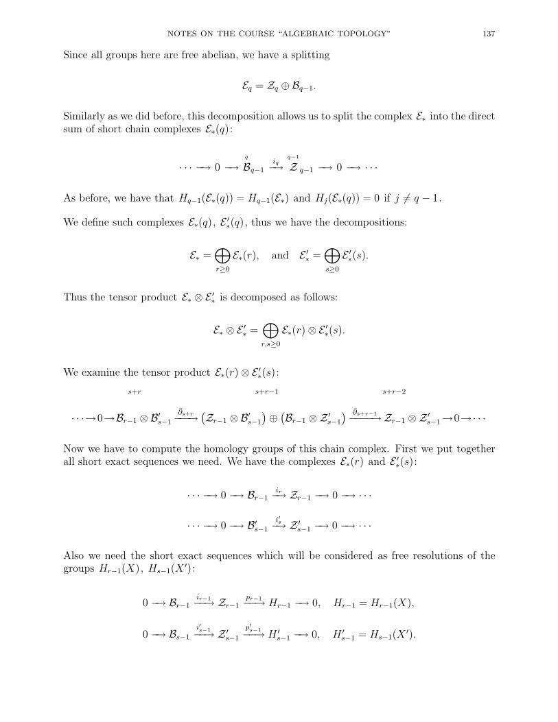
NOTES ON THE COURSE “ALGEBRAIC TOPOLOGY” 137
Since all groups here are free abelian, we have a splitting
Eq = Zq ⊕ Bq−1.
Similarly as we did before, this decomposition allows us to split the complex E∗ into the directsum of short chain complexes E∗(q):
· · · −→ 0 −→q
Bq−1iq−→
q−1
Z q−1 −→ 0 −→ · · ·
As before, we have that Hq−1(E∗(q)) = Hq−1(E∗) and Hj(E∗(q)) = 0 if j 6= q − 1.
We define such complexes E∗(q), E ′∗(q), thus we have the decompositions:
E∗ =⊕
r≥0
E∗(r), and E ′∗ =⊕
s≥0
E ′∗(s).
Thus the tensor product E∗ ⊗ E ′∗ is decomposed as follows:
E∗ ⊗ E ′∗ =⊕
r,s≥0
E∗(r)⊗ E ′∗(s).
We examine the tensor product E∗(r)⊗ E ′∗(s):s+r s+r−1 s+r−2
· · ·→0→Br−1 ⊗ B′s−1
∂s+r−−−→(Zr−1 ⊗ B′
s−1
)⊕(Br−1 ⊗Z ′
s−1
) ∂s+r−1−−−−→Zr−1 ⊗ Z ′s−1→0→· · ·
Now we have to compute the homology groups of this chain complex. First we put togetherall short exact sequences we need. We have the complexes E∗(r) and E ′∗(s):
· · · −→ 0 −→ Br−1ir−→ Zr−1 −→ 0 −→ · · ·
· · · −→ 0 −→ B′s−1
i′s−→ Z ′s−1 −→ 0 −→ · · ·
Also we need the short exact sequences which will be considered as free resolutions of thegroups Hr−1(X), Hs−1(X
′):
0 −→ Br−1ir−1−−→ Zr−1
pr−1−−→ Hr−1 −→ 0, Hr−1 = Hr−1(X),
0 −→ Bs−1
i′s−1−−→ Z ′s−1
p′s−1−−→ H ′s−1 −→ 0, H ′
s−1 = Hs−1(X′).

138 BORIS BOTVINNIK
Consider the following diagram:
(79)
0
?
0
?
0
?0→ Br−1 ⊗ B′
s−1
?Id
Zr−1 ⊗ B′s−1 ⊕ Br−1 ⊗ B′
s−1
?1⊗1⊕1⊗i′s−1
Zr−1 ⊗ B′s−1
?1⊗i′s−1
→ 0-dr+s -dr+s−1
0→ Br−1 ⊗ B′s−1
?
Zr−1 ⊗ B′s−1 ⊕ Br−1 ⊗Z ′
s−1
?0⊕1⊗p′s−1
Zr−1 ⊗Z ′s−1
?1⊗p′s−1
→ 0-∂s+r -∂s+r−1
0 0
?
Br−1 ⊗H ′s−1
?
Zr−1 ⊗H ′s−1
?
→ 0- - -ir−1⊗1
0 0 0
Here the homomorphisms ∂s+r , ∂s+r are given by
∂s+r(b⊗ b′) = (ir−1b)⊗ b′ ⊕ (−1)rb⊗ (i′s−1b′) ∈ Zr−1 ⊗ B′
s−1 ⊕ Br−1 ⊗ Z ′s−1,
∂s+r−1(z ⊗ b′ ⊕ b⊗ z′) = (−1)r−1z ⊗ (i′s−1b′) + (ir−1b)⊗ z′ ∈ Zr−1 ⊗ Z ′
s−1.
The homomorphisms dr+s , dr+s−1 are defined similarly:
ds+r(b⊗ b′) = (ir−1b)⊗ b′ ⊕ (−1)rb⊗ b′ ∈ Zr−1 ⊗ B′s−1 ⊕ Br−1 ⊗ B′
s−1,
ds+r−1(z ⊗ b′1 ⊕ b⊗ b′2) = (−1)r−1z ⊗ b′1 + (ir−1b)⊗ b′2 ∈ Zr−1 ⊗ B′s−1.
It is easy to check that the diagram (79) commutes and the columns are exact. We considerthe diagram (79) as a short exact sequence of chain complexes. We notice that the sequence
0→ Br−1 ⊗ B′s−1
dr+s−−−→ Zr−1 ⊗ B′s−1 ⊕ Br−1 ⊗ B′
s−1
dr+s−1−−−−→ Zr−1 ⊗ B′s−1 → 0
is exact. Thus the homology groups of this complex are trivial. On the other hand, thehomology groups of the complex
0 −→ Br−1 ⊗H ′s−1
ir−1⊗1−−−−→ Zr−1 ⊗H ′s−1 → 0
are equal to Hr−1 ⊗H ′s−1 (in degree r + s− 2), and Tor(Hr−1, H
′s−1) (in degree r + s − 1)
and zero otherwise. The long exact sequence in homology groups corresponding to the shortexact sequence of chain complexes (79) immediately implies that
Hj(E∗(r)⊗ E ′∗(s)) =
Hr−1 ⊗H ′s−1 if j = r + s− 2,
Tor(Hr−1, H′s−1) if j = r + s− 1,
0 else.
Now it is enough to assemble the homology groups of the chain complex E∗ ⊗ E ′∗ out ofthe homology groups of the chain complexes E∗(s) ⊗ E ′∗(r) to get the desired formula. Thisconcludes the proof of Theorem 15.4.
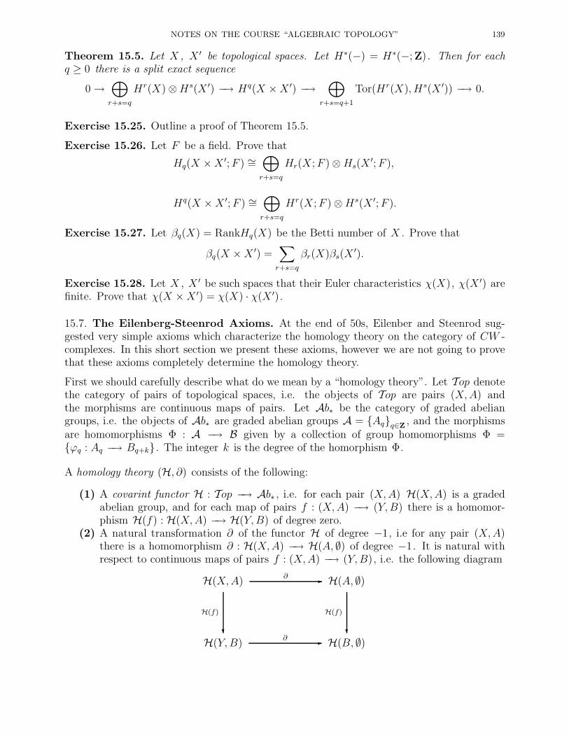
NOTES ON THE COURSE “ALGEBRAIC TOPOLOGY” 139
Theorem 15.5. Let X , X ′ be topological spaces. Let H∗(−) = H∗(−;Z). Then for eachq ≥ 0 there is a split exact sequence
0→⊕
r+s=q
Hr(X)⊗Hs(X ′) −→ Hq(X ×X ′) −→⊕
r+s=q+1
Tor(Hr(X), Hs(X ′)) −→ 0.
Exercise 15.25. Outline a proof of Theorem 15.5.
Exercise 15.26. Let F be a field. Prove that
Hq(X ×X ′;F ) ∼=⊕
r+s=q
Hr(X;F )⊗Hs(X′;F ),
Hq(X ×X ′;F ) ∼=⊕
r+s=q
Hr(X;F )⊗Hs(X ′;F ).
Exercise 15.27. Let βq(X) = RankHq(X) be the Betti number of X . Prove that
βq(X ×X ′) =∑
r+s=q
βr(X)βs(X′).
Exercise 15.28. Let X , X ′ be such spaces that their Euler characteristics χ(X), χ(X ′) arefinite. Prove that χ(X ×X ′) = χ(X) · χ(X ′).
15.7. The Eilenberg-Steenrod Axioms. At the end of 50s, Eilenber and Steenrod sug-gested very simple axioms which characterize the homology theory on the category of CW -complexes. In this short section we present these axioms, however we are not going to provethat these axioms completely determine the homology theory.
First we should carefully describe what do we mean by a “homology theory”. Let Top denotethe category of pairs of topological spaces, i.e. the objects of Top are pairs (X,A) andthe morphisms are continuous maps of pairs. Let Ab∗ be the category of graded abeliangroups, i.e. the objects of Ab∗ are graded abelian groups A = Aqq∈Z
, and the morphismsare homomorphisms Φ : A −→ B given by a collection of group homomorphisms Φ =ϕq : Aq −→ Bq+k . The integer k is the degree of the homorphism Φ.
A homology theory (H, ∂) consists of the following:
(1) A covarint functor H : Top −→ Ab∗ , i.e. for each pair (X,A) H(X,A) is a gradedabelian group, and for each map of pairs f : (X,A) −→ (Y,B) there is a homomor-phism H(f) : H(X,A) −→ H(Y,B) of degree zero.
(2) A natural transformation ∂ of the functor H of degree −1, i.e for any pair (X,A)there is a homomorphism ∂ : H(X,A) −→ H(A, ∅) of degree −1. It is natural withrespect to continuous maps of pairs f : (X,A) −→ (Y,B), i.e. the following diagram
H(X,A)
?
H(f)
H(A, ∅)
?
H(f)
-∂
H(Y,B) H(B, ∅)-∂
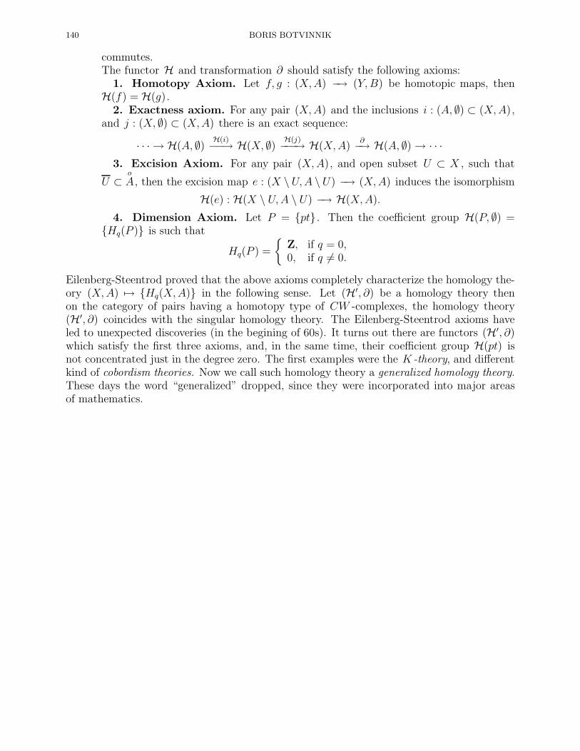
140 BORIS BOTVINNIK
commutes.The functor H and transformation ∂ should satisfy the following axioms:
1. Homotopy Axiom. Let f, g : (X,A) −→ (Y,B) be homotopic maps, thenH(f) = H(g).
2. Exactness axiom. For any pair (X,A) and the inclusions i : (A, ∅) ⊂ (X,A),and j : (X, ∅) ⊂ (X,A) there is an exact sequence:
· · · → H(A, ∅) H(i)−−→ H(X, ∅) H(j)−−−→ H(X,A)∂−→ H(A, ∅)→ · · ·
3. Excision Axiom. For any pair (X,A), and open subset U ⊂ X , such that
U ⊂o
A, then the excision map e : (X \U,A \U) −→ (X,A) induces the isomorphism
H(e) : H(X \ U,A \ U) −→ H(X,A).
4. Dimension Axiom. Let P = pt . Then the coefficient group H(P, ∅) =Hq(P ) is such that
Hq(P ) =
Z, if q = 0,0, if q 6= 0.
Eilenberg-Steentrod proved that the above axioms completely characterize the homology the-ory (X,A) 7→ Hq(X,A) in the following sense. Let (H′, ∂) be a homology theory thenon the category of pairs having a homotopy type of CW -complexes, the homology theory(H′, ∂) coincides with the singular homology theory. The Eilenberg-Steentrod axioms haveled to unexpected discoveries (in the begining of 60s). It turns out there are functors (H′, ∂)which satisfy the first three axioms, and, in the same time, their coefficient group H(pt) isnot concentrated just in the degree zero. The first examples were the K -theory, and differentkind of cobordism theories. Now we call such homology theory a generalized homology theory.These days the word “generalized” dropped, since they were incorporated into major areasof mathematics.

NOTES ON THE COURSE “ALGEBRAIC TOPOLOGY” 141
16. Some applications
16.1. The Lefschetz Fixed Point Theorem. We still start with some algebraic construc-tions. Let A be a finitely generated abelian group. Denote F (A) the free part of A, so thatA = F (A) ⊕ T (A), where T (A) is a maximum torsion subgroup of A. Let ϕ : A −→ A bean endomorphism of A. We define F (ϕ) : F (A) −→ F (A) by composition:
F (ϕ) : F (A)inclusion−−−−−−→ A
ϕ−→ Aprojection−−−−−−−→ F (A).
The homomorphism F (ϕ) is an endomorphism of the free abelian finitely generated groupF (A). Hence the trace Tr(F (ϕ)) ∈ Z is well-defined. We define Tr(ϕ) = Tr(F (ϕ)). Nowlet A = Aqq≥0 be a finitely generated graded abelian group, i.e. each group Aq is finitelygenerated. A homomorphism Φ : A −→ B of two graded abelian groups is a collection ofhomomorphisms ϕq : Aq −→ Bq−k (the number k is the degree of Φ).
Now let A = Aqq≥0 be a finitely generated graded abelian group, and let
Φ = ϕq : A −→ Abe an endomorphism of degree zero. We assume that F (Aq) = 0 for q ≥ n (for some n). Wedefine the Lefschetz number Lef(Φ) of the endomorphism Φ by the formula:
Lef(Φ) =∑
q≥0
(−1)qTr(ϕq).
Clearly we have several natural examples of such endomorphisms. The main example we aregoing to work with is the following. Let X be a finite CW -complex, and f : X −→ X be amap. Then there are the induced endomorphisms of degree zero
f# : E∗(X) −→ E∗(X), f∗ : H∗(X) −→ H∗(X),
where E∗(X) = Eq(X) , H∗(X) = Hq(X) are considered as graded abelian groups.
Claim 16.1. Let C be a chain complex, C = Cq, such that Cq = 0 for q ≥ n (for somen). Let ϕ : C −→ C be a chain map, and ϕ∗ : H∗C −→ H∗C be the induced homomorphismin homology groups. Then
Lef(ϕ) = Lef(ϕ∗).
Exercise 16.1. Prove Claim 16.1.
Let f : X −→ X be a map of finite CW -complex to itself. We define the Lefschetz numberLef(f) = Lef(f∗), where f∗ : H∗(X) −→ H∗(X) is the induced homomorphism in homologygroups. Clearly the Lefschetz number Lef(f) depends on the homotopy class of f .
Theorem 16.1. (Lefschetz Fixed Point Theorem) Let X be a finite CW -complex andf : X −→ X be a map such that Lef(f) 6= 0. Then f has a fixed point, i.e. such a pointx0 ∈ X that f(x0) = x0 .
Proof. First we recall that a finite CW -complex X may be embedded as a compact subspaceinto the Euclidian space Rn for some n. In particular, the metric on X (which is the inducedmetric from Rn ) determines the original topology on X . Let d(x, x′) be the distance functioninduced by this metric.
142 BORIS BOTVINNIK
Assume that f(x) 6= x for each point x ∈ X . Since X is a compact, there exists a positivenumber ǫ > 0 so that d(f(x), x) > ǫ for all x ∈ X . For every cell eq of X , we use ahomeomorphism ∆q ∼= eq to define new CW -structure on X as follows. We find a barycenticsubdivision of ∆q such that
diam(∆) < ǫ/9, and diam(f(∆)) < ǫ/9
for each simplex ∆ of that barycentic subdivision. The simplices ∆ of this barycentic subdi-vision define new CW -structure on X . Let
σqj
be the cells of this CW -structure on X .For each cell σq0 we define the subcomplex
Eq0 =
⋃
σj∩σq0 6=∅
σj.
Notice that the diameter diam(Eq0) < 4ǫ/9. Indeed, let x, x′ ∈ Eq
0 . Choose x0 ∈ σq0 . Thend(x, x0) < 2ǫ/9, and d(x′, x0) < 2ǫ/9. Thus
d(x, x′) ≤ d(x, x0) + d(x′, x0) < 4ǫ/9.
Clearly diam(f(Eq0)) < 4ǫ/9 as well. Now it is clear that d(Eq
0 , f(Eq0)) > ǫ − 8ǫ/9 = ǫ/9.
HenceEq
0 ∩ f(Eq0) = ∅.
Now we use the cellular approximation Theorem 5.5 where we constructed a cellular mapf ′ ∼ f . It is easy to see that f ′(σq0) ⊂ f(Eq
0) by construction we gave in the proof ofTheorem 5.5. Thus σq0∩f ′(σq0) = ∅ . Now consider the homomorphism f ′
# : Eq(X) −→ Eq(X).We have that
f ′#(σq0) =
∑
i
λiσqi , where σqi 6= σq0.
Hence Tr(f ′#) = 0 for each q ≥ 0, and
0 = Lef(f ′#) = Lef(f#) = Lef(f∗) = Lef(f).
This concludes the proof.
Corollary 16.2. Let X be a finite contractible CW -complex. Then any map f : X −→ Xhas a fixed point.
Exercise 16.2. Prove Corollary 16.2.
A continuous family ϕt : X −→ X of maps is called a flow if the following conditions aresatisfied:
(a) ϕ0 = IdX ,(b) ϕt is a homeomorphism for any t ∈ R ,(c) ϕs+t(x) = ϕs ϕt(x).
It is convenient to treat a flow ϕt as a map ϕ : X ×R −→ R , where ϕ(x, t) = ϕt(x). A flowis also known as one-parameter group of homeomorphisms. The following statement is notvery hard to prove, however, it provides an important link to analysis.
Theorem 16.3. Let X be a finite CW -complex with χ(X) 6= 0, and ϕt : X −→ X be aflow. Then there exists a point x0 ∈ X so that ϕt(x0) = x0 for all t ∈ R.

NOTES ON THE COURSE “ALGEBRAIC TOPOLOGY” 143
Proof. By definition, each map ϕt ∼ IdX . Thus Lef(ϕt) = Lef(IdX) = χ(X) 6= 0. Thus
there exists a fixed point x(t)0 of ϕt for each t. Let
An =x ∈ X | ϕ1/2n(x) = x
.
Clearly An ⊃ An+1 , and each An is a closed subset (as the intersection of the diagonal∆(X) = (x, x) ⊂ X × X and the graph Γ(ϕ1/2n) =
(x, ϕ1/2n(x))
⊂ X × X ). Thus
F = ∩nAn is not empty. Let x ∈ F . Clearly x is a fixed point for any ϕm/2n . Since thenumbers m/2n are dense in R , x is a fixed point for ϕt for any t ∈ R .
Remark. Let X = Mn be a smooth manifold, and assume a flow ϕ : Mn × R −→ Mn isa smooth flow, i.e. the map ϕ is smooth, and ϕt is a diffeomorphism. We can even assumethat the flow ϕ is defined only for t ∈ (−ǫ, ǫ). Let x ∈Mn , the
dϕ0(x)
dt= lim
τ→0
ϕτ (x)− ϕ0(x)
τ= lim
τ→0
ϕτ (x)− xτ
is a tangent vector to Mn at the point x, and the correspondence
v : x 7→ dϕ0(x)
dt
defines a smooth tangent vector field v(x) on Mn . Theorem 16.3 implies that if χ(Mn) 6= 0,then there is no tangent vector field on M without zero points. Actually, a generic tangentvector field always has only isolated nondegenerated zero points, so that each zero point hasindex ±1. The Euler-Poincare Theorem states that the sum of those indices is exactly theEuler characteristic χ(M). 10
Exercise 16.3. Let f : RP2n −→ RP2n be a map. Prove that f always has a fixed point.Give an example that the above statement fails for a map f : RP2n+1 −→ RP2n+1 .
Exercise 16.4. Let n 6= k . Prove that Rn is not homeomorphic to Rk .
Exercise 16.5. Let f : Sn −→ Sn be a map, and deg(f) be the degree of f . Prove thatLef(f) = 1 + (−1)n deg(f).
Exercise 16.6. Prove that there is no tangent vector field v(x) on the sphere S2n such thatv(x) 6= 0 for all x ∈ S2n . (Compare with Lemma 13.9.)
16.2. The Jordan-Brouwer Theorem. This is a classical result about an embedded sphereSn−1 ⊂ Sn .
Theorem 16.4. (The Jordan-Brouwer Theorem) Let Sn−1 ⊂ Sn be an embedded sphere inSn . Then the complement X = Sn \Sn−1 has two path-connected components: X = X1⊔X2 ,where X1 , X2 are open in Sn . Furthermore, ∂X1 = ∂X2 = Sn−1 .
First we prove a technical result.
10 See J. Milnor, Differential topology, mimeographic notes. Princeton: Princeton University Press, 1958,for details.

144 BORIS BOTVINNIK
Lemma 16.5. Let K ⊂ Sn be homeomorphic to the cube Ik , 0 ≤ k ≤ n. Then
Hq(Sn \K) = 0 for all q ≥ 0 .
Proof. Induction on k . The case k = 0 is obvious. Assume that the statement holdsfor all 0 ≤ k ≤ m − 1, and let K is homeomorphic to Im . We choose a decompositionK = L × I , where L is homeomorphic to Im−1 . Let K1 = L × [0, 1
2], and K2 = L × [1
2, 1].
Then K1 ∩K2 = L×
12
∼= Im−1 . By induction,
Hq(Sn \K1 ∩K2) = 0 for all q ≥ 0 .
We notice that the sets Sn \K1 , Sn \K2 are both open in Sn . Thus we can use the Mayer-Vietoris exact sequence
· · · → Hq(Sn \K1 ∪K2) −→ Hq(S
n \K1)⊕ Hq(Sn \K2) −→ Hq(S
n \K1 ∩K2)→ · · ·Thus we have that
Hq(Sn \K1 ∪K2) ∼= Hq(S
n \K1)⊕ Hq(Sn \K2).
Assume that Hq(Sn \K1 ∪K2) 6= 0, and z0 ∈ Hq(S
n \K1 ∪K2), z0 6= 0. Then z0 = (z′0, z′′0 ),
thus there exists z1 6= 0 in the group Hq(Sn \K1) or Hq(S
n\K2). Let, say, z1 ∈ Hq(Sn \K1),
z1 6= 0. Then we repeat the argument for K1 , and obtain the sequence
K ⊃ K(1) ⊃ K(2) ⊃ K(2) ⊃ · · ·such that
(1) K(s) is homeomorphic to Im ,(2) the inclusion is : Sn \ K ⊂ Sn \ K(s) takes the element z to a nonzero element
zs ∈ Hq(Sn \K(s)),
(3) the intersection⋂
s
K(s) is homeomorphic to Im−1 .
We have that any compact subset C of Sn \⋂
s
K(s) lies in Sn \K(s) for some s, we obtain
that Cq(Sn \⋂
s
K(s)) = lim−→sCq(S
n \K(s)), and, respectively,
Hq(Sn \⋂
s
K(s)) = lim−→sHq(S
n \K(s)).
By construction, there exists an element z∞ ∈ Hq(Sn \⋂sK
(s)), z∞ 6= 0. Contradiction tothe inductive assumption.
Theorem 16.6. Let Sk ⊂ Sn , 0 ≤ k ≤ n− 1. Then
(80) Hq(Sn \ Sk) ∼=
Z, if q = n− k − 1,0 if q 6= n− k − 1.
Proof. Induction on k . If k = 0, then Sn \ S0 is homotopy equivalent to Sn−1 . Thus theformula (80) holds for k = 0. Let k ≥ 1, then Sk = Dk
+ ∪Dk− , where Dk
+ , Dk− are the south
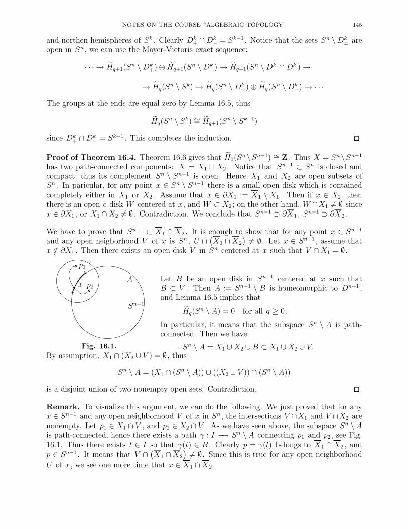
NOTES ON THE COURSE “ALGEBRAIC TOPOLOGY” 145
and northen hemispheres of Sk . Clearly Dk+ ∩Dk
− = Sk−1 . Notice that the sets Sn \Dk± are
open in Sn , we can use the Mayer-Vietoris exact sequence:
· · · → Hq+1(Sn \Dk
+)⊕ Hq+1(Sn \Dk
−)→ Hq+1(Sn \Dk
+ ∩Dk−)→
→ Hq(Sn \ Sk)→ Hq(S
n \Dk+)⊕ Hq(S
n \Dk−)→ · · ·
The groups at the ends are equal zero by Lemma 16.5, thus
Hq(Sn \ Sk) ∼= Hq+1(S
n \ Sk−1)
since Dk+ ∩Dk
− = Sk−1 . This completes the induction.
Proof of Theorem 16.4. Theorem 16.6 gives that H0(Sn \Sn−1) ∼= Z. Thus X = Sn \Sn−1
has two path-connected components: X = X1 ⊔ X2 . Notice that Sn−1 ⊂ Sn is closed andcompact; thus its complement Sn \ Sn−1 is open. Hence X1 and X2 are open subsets ofSn . In paricular, for any point x ∈ Sn \ Sn−1 there is a small open disk which is containedcompletely either in X1 or X2 . Assume that x ∈ ∂X1 := X1 \ X1 . Then if x ∈ X2 , thenthere is an open ǫ-disk W centered at x, and W ⊂ X2 ; on the other hand, W ∩X1 6= ∅ sincex ∈ ∂X1 , or X1 ∩X2 6= ∅ . Contradiction. We conclude that Sn−1 ⊃ ∂X1 , Sn−1 ⊃ ∂X2 .
We have to prove that Sn−1 ⊂ X1 ∩ X2 . It is enough to show that for any point x ∈ Sn−1
and any open neigborhood V of x is Sn , U ∩(X1 ∩X2
)6= ∅ . Let x ∈ Sn−1 , assume that
x /∈ ∂X1 . Then there exists an open disk V in Sn centered at x such that V ∩X1 = ∅ .
Sn−1
p1
Ap2x
Fig. 16.1.
Let B be an open disk in Sn−1 centered at x such thatB ⊂ V . Then A := Sn−1 \ B is homeomorphic to Dn−1 ,and Lemma 16.5 implies that
Hq(Sn \ A) = 0 for all q ≥ 0 .
In particular, it means that the subspace Sn \ A is path-connected. Then we have:
Sn \ A = X1 ∪X2 ∪ B ⊂ X1 ∪X2 ∪ V.By assumption, X1 ∩ (X2 ∪ V ) = ∅ , thus
Sn \ A = (X1 ∩ (Sn \ A)) ∪ ((X2 ∪ V )) ∩ (Sn \ A))
is a disjoint union of two nonempty open sets. Contradiction.
Remark. To visualize this argument, we can do the following. We just proved that for anyx ∈ Sn−1 and any open neighborhood V of x in Sn , the intersections V ∩X1 and V ∩X2 arenonempty. Let p1 ∈ X1 ∩ V , and p2 ∈ X2 ∩ V . As we have seen above, the subspace Sn \ Ais path-connected, hence there exists a path γ : I −→ Sn \ A connecting p1 and p2 , see Fig.16.1. Thus there exists t ∈ I so that γ(t) ∈ B . Clearly p = γ(t) belongs to X1 ∩X2 , andp ∈ Sn−1 . It means that V ∩
(X1 ∩X2
)6= ∅ . Since this is true for any open neighborhood
U of x, we see one more time that x ∈ X1 ∩X2 .
146 BORIS BOTVINNIK
16.3. The Brouwer Invariance Domain Theorem. This is also a classical result.
Theorem 16.7. (The Brouwer Invariance Domain Theorem) Let U and V be subsets of Sn ,so that U and V are homeomorphic, and U are open in Sn . Then V is also open in Sn .
Proof. Let h : U −→ V be a homeomorphism, and h(x) = y . Since U is an open subset ofSn , there exsits a neighborhood A of x in U , so that A is homeomorphic to the disk Dn .Let B = ∂A. Denote A′ = h(A) ⊂ V , B′ = h(B) ⊂ V . By Lemma 16.5 the subset Sn \ A′
is path-connected, and by Theorem 16.4 the subset Sn \ B′ has two path-components. Wehave that
Sn \B′ = (Sn \ A′) ∪ (A′ \B′),
and the sets Sn \ A′ and A′ \ B′ are path-connected, then they are the path-components ofSn \ B′ . Thus A′ \ B′ is open in Sn . Since A′ \ B′ ⊂ V , and y ∈ V is an arbitrary point,the set V is open in Sn .
16.4. Borsuk-Ulam Theorem. First we introduce new long exact sequence in homologywhich corresponds to a two-fold covering p : T → X . We observe that the chain mapp# : C(T ;Z/2)→ C(X;Z/2) fits into the following exact sequence of chain complexes:
(81) 0→ C(X;Z/2)τ−→ C(T ;Z/2)
p#−→ C(X;Z/2)→ 0.
Here the chain map τ : C(X;Z/2) → C(T ;Z/2) is defined as follows. Let h : ∆q → X be
a generator of Cq(X;Z/2). Let ∆q = (v0, . . . , vq), and x0 = h(v0). Let x(1)0 , x
(2)0 ∈ T be
two lifts of the point x0 . Then, since ∆q is simply-connected, there exist exactly two lifts
h(i) : ∆q → T , i = 1, 2 such that h(1)(v0) = x(1)0 and h(2)(v0) = x
(2)0 . Then
τ(h : ∆q → X) := (h(1) : ∆q → T ) + (h(2) : ∆q → T ).
The homomorphism τ is sometimes called a transfer homomorphism. On the other hand,it easy to see that the kernel of p# : Cq(T ;Z/2) → Cq(X;Z/2) is generated by the sums
(h(1) : ∆q → T ) + (h(2) : ∆q → T ). Thus the short exact sequence (81) gives a long exactsequence in homology groups (with Z/2 coefficients):
(82) · · · → Hq(X;Z/2)τ∗−→ Hq(T ;Z/2)
p∗−→ Hq(X;Z/2)∂−→ Hq−1(X;Z/2)→ · · ·
We will use the long exact sequence (82) to prove the following result, known as Borsuk-UlamTheorem.
Theorem 16.8. Let f : Sn → Sn be a map such that f(−x) = −f(x) (an “odd map”).Then deg f is odd.
Proof. Consider the long exact sequence (82) for the covering Sn → RPn :
0→ Hn(RPn)τ∗−→ Hn(S
n)p∗−→ Hn(RPn)
∂−→ Hn−1(RPn)→ 0→ · · ·
· · · → 0→ Hq(RPn)∂−→ Hq−1(RPn)→ 0→ · · ·
· · · → 0→ H1(RPn)∂−→ H0(RPn)→ H0(S
n)p∗−→ H0(RPn)→ 0

NOTES ON THE COURSE “ALGEBRAIC TOPOLOGY” 147
The exactness forces that the homomorphisms
τ∗ : Hn(RPn)→ Hn(Sn),
∂ : Hq(RPn)→ Hq−1(RPn), q = n, n− 1, . . . , 1,
p∗ : H0(Sn)→ H0(RPn)
to be isomorphisms, and p∗ : Hq(Sn)→ Hq(RPn) to be zero for q > 0.
Now let f : Sn → Sn be a map such that f(−x) = −f(x). Then it induces a quotient mapf : RPn → RPn , such that the diagram
Sn
?
p
Sn
?
p
-f
RPn RPn-f
Now we notice that f∗ : H0(Sn) → H0(S
n) f∗ : H0(RPn) → H0(RPn) are isomorphisms,then we use naturality of the exact sequence (82) to get the commutative diagrams
Hq(RPn)
?
f∗
Hq−1(RPn)
?
f
-∂
Hq(RPn) Hq−1(RPn)-∂
Hn(RPn)
?
f∗
Hn(Sn)
?
f∗
-τ
Hn(RPn) Hn(Sn)-τ
.
for q = 1, . . . n. In particular, we obtain that f∗ : Hn(Sn;Z/2)→ Hn(S
n;Z/2) is an isomor-phism. On the other hand, we know that for integral homology groups
f∗ : Hn(Sn)→ Hn(S
n)
is a multiplication by the degree deg f . We obtain that after reduction modulo two f∗ isisomorphism:
Hn(Sn;Z)
?
pr
Hn(Sn;Z)
?
pr
-f∗
Hn(Sn;Z/2) Hn(S
n;Z/2)-∼=
Thus the degree deg f must be odd.
Exercise 16.7. Let 0 ≤ p, q ≤ n− 1, and the wedge Sp ∨ Sq is embedded to Sn . Computethe homology groups Hq(S
n \ (Sp ∨ Sq)).
148 BORIS BOTVINNIK
Exercise 16.8. Prove that for each n ≥ 1 there exists a space X with
Hq(X) =
Z/m, if q = n,
0, if q 6= n.
Exercise 16.9. Let H = Hq be a graded abelian group. We assume that Hq = 0 forq < 0, and H0 is a free abelian. Prove that there exists a space X such that Hq(X) = Hq
for all q . In particular, construct a space X with the homology groups:
Hq(X) =
Z[1
p], if q = n,
0, if q 6= n.
NOTES ON THE COURSE “ALGEBRAIC TOPOLOGY” 149
17. Cup product in cohomology.
17.1. Ring structure in cohomology. The homology groups are more “geometric” thanthe cohomology. However, there is a natural ring structure in cohomology groups which isvery useful. The Kunneth formula gives natural homomorphism
m : Hk(X;Z)⊗H l(X;Z) −→ Hk+l(X ×X;Z)
Consider the diagonal map ∆ : X −→ X × X which sends x to the pair (x, x). Then wehave the composition
Hk(X;Z)⊗H l(X;Z)m−→ Hk+l(X ×X;Z)
∆∗
−−→ Hk+l(X;Z).
which gives the product structure in cohomology. The way we defined this product does notallow us to compute actual ring structure for particular spaces. What we are going to do isto work out this in detail starting with cup-product at the level of singular cochains.
17.2. Definition of the cup-product. First we need some notations. We identify a simplex∆q with one given by its vertices (v0, . . . , vq) in Rq+1 . Let g : ∆q −→ X be a map. It isconvenient to use symbol (v0, . . . , vq) to denote the singular simplex g : ∆q −→ X , and, say,(v0, . . . , vs) the restriction g|(v0,...,vs) .
Let R be a commutative ring with unit. We consider cohomology groups with coefficients inR . The actual examples we will elaborate are when R = Z, Z/p, Q, R . Let ϕ ∈ Ck(X),ψ ∈ C l(X) be singular cochains, and f : ∆k+l −→ X be a singular simplex. We define thecochain ϕ ∪ ψ ∈ Ck+l(X) as follows:
〈ϕ ∪ ψ, (v0, . . . , vk+l)〉 = (ϕ ∪ ψ)(v0, . . . , vk+l) := ϕ(v0, . . . , vk)ψ(vk, . . . , vk+l).
To see that the cup-product at the level of cochains induces a product in cohomology groups,we have to undestand the coboundary homomorphism on ϕ ∪ ψ .
Lemma 17.1. Let ϕ ∈ Ck(X), ψ ∈ C l(X). Then
δ(ϕ ∪ ψ) = δϕ ∪ ψ + (−1)kϕ ∪ δψ.
Proof. Let g : ∆k+l+1 −→ X be a singular simplex. We compute 〈δϕ∪ψ, g〉 and 〈ϕ∪δψ, g〉 :
(83)
〈δϕ ∪ ψ, g〉 =
k+1∑
j=0
(−1)jϕ(v0, . . . , vj, . . . , vk+1)ψ(vk+1, . . . , vk+l+1),
〈ϕ ∪ δψ, g〉 =
k+l+1∑
j=k
(−1)j+kϕ(v0, . . . , vk)ψ(vk, . . . , vj, . . . , vk+l+1).
= (−1)kk+l+1∑
j=k
(−1)jϕ(v0, . . . , vk)ψ(vk, . . . , vj, . . . , vk+l+1).
150 BORIS BOTVINNIK
Consider the following terms in (83):
(−1)k+1ϕ(v0, . . . , . . . , vk)ψ(vk+1, . . . , vk+l+1)
(−1)kϕ(v0, . . . , . . . , vk)ψ(vk+1, . . . , vk+l+1)
The first one corresponds to j = k + 1 in the formula for 〈δϕ ∪ ψ, g〉 , and the second onecorresponds to j = k in the formula for 〈ϕ ∪ δψ, g〉 . Clearly they cancel each other, and wehave that
(84)
〈δϕ ∪ ψ + (−1)kϕ ∪ δψ, g〉 =
k∑
j=0
(−1)jϕ(v0, . . . , vj, . . . , vk+1)ψ(vk+1, . . . , vk+l+1)
+
k+l+1∑
j=k+1
(−1)jϕ(v0, . . . , vk)ψ(vk, . . . , vj, . . . , vk+l+1)
=k+l+1∑
j=0
(−1)j(ϕ ∪ ψ)(v0, . . . , vj, . . . , vk+l+1)
= 〈ϕ ∪ ψ, ∂g〉 = 〈δ(ϕ ∪ ψ), g〉.
This concludes the proof.
Now it is clear that the cup product of two cocyles is a cocycle, and the cup-product of cocycleand coboundary is a coboundary. We conclude that the cup-product in the cochain groupsinduces the cup-product in cohomology:
∪ : Hk(X;R)×H l(X;R) −→ Hk+l(X;R),
where R is a commutative ring. The cup-product induces the ring structure on H∗(X;R). LetK∗ =
⊕Kj be a graded R-module, with K0 = R and Kj = 0 for j < 0. We say that K∗ is a
graded algebra over R if there is a product µ : K∗⊗K∗ −→ K∗ so that µ : Kk⊗Kℓ −→ Kk+ℓ ,and the unit 1 ∈ R = K0 is the unit of the product µ , i.e. µ(1 ⊗ a) = µ(a ⊗ 1) = a. Wesay that (K∗, µ) is a graded commutative R-algebra if µ(a ⊗ b) = (−1)kℓµ(b ⊗ a), wheredeg a = k , deg b = ℓ.
Claim 17.1. Let R be a commutative ring. Then H∗(X;R) is a graded commutative R-algebra.
Construction. Let f : ∆q −→ X be a singular simplex, and the simplex ∆q is given by itsvertices (v0, . . . , vq). Consider the singular simplex f : ∆q −→ X , where ∆q = (vq, . . . , v0),and
f : ∆q T−→ ∆q f−→ X

NOTES ON THE COURSE “ALGEBRAIC TOPOLOGY” 151
where T is given by the linear isomorphism T : Rq+1 −→ Rq+1 sending vertices (v0, . . . , vq)to (vq, . . . , v0) respectively. Clearly as a linear map, T is given by the matrix
T =
0 0 · · · 0 10 0 · · · 1 0...
......
......
...0 1 · · · 0 01 0 · · · 0 0
which has determinant detT = (−1)q(q+1)
2 . Thus T induces the chain map
t : C∗(X) −→ C∗(X)
sending a generator f : ∆q −→ X to the generator f : ∆q −→ X .
Exercise 17.1 Prove that there is a chain homotopy between t and (−1)q(q+1)
2 Id .
The homomorphism t : C∗(X) −→ C∗(X) induces the homomorphism
t∗ : C∗(X;R) −→ C∗(X;R).
Clearly in cohomology the homomorphism t∗ coincides with
(−1)q(q+1)
2 Id : Hq(X;R) −→ Hq(X;R).
Proof of Claim 17.1. Let ϕ ∈ Ck(X;R), ψ ∈ C l(X;R), and f : ∆k+l −→ X be a singularsimplex. As above, we denote the singular simplex by its vertices (v0, . . . , vk+l). We have:
(ϕ ∪ ψ)(v0, . . . , vk+l) = ϕ(v0, . . . , vk)ψ(vk, . . . , vk+l)
= (−1)k(k+1)
2 ϕ(vk, . . . , v0)(−1)l(l+1)
2 ψ(vk+l, . . . , vk)
= (−1)k(k+1)
2+
l(l+1)2 ψ(vk+l, . . . , vk)ϕ(vk, . . . , v0)
= (−1)k(k+1)
2+
l(l+1)2 (ψ ∪ ψ)(vk+l, . . . , v0)
= (−1)k(k+1)
2+ l(l+1)
2 (−1)(k+l)(k+l+1)
2 (ψ ∪ ψ)(v0, . . . , vk+l)
= (−1)kl(ψ ∪ ϕ)(v0, . . . , vk+l).
Here we have identified singular simplex g = g T with the map (−1)q(q+1)
2 g for a singularsimplex g : ∆q −→ X .
Theorem 17.2. (Properties of the cup-product) Let X be a space and R a commutative ringwith unit. Let γ ∈ Hq(X;R), γ′ ∈ Hq′(X;R), γ′′ ∈ Hq′′(X;R) j = 1, 2, 3 be any elements.Then
(1) γ ∪ γ′ = (−1)qq′
γ′ ∪ γ ;(2) (γ ∪ γ′) ∪ γ′′ = γ ∪ (γ′ ∪ γ′′);(3) f ∗(γ ∪ γ′) = (f ∗γ) ∪ (f ∗γ′) and α∗(γ ∪ γ′) = (α∗γ) ∪ (α∗γ′) for any map f : X → X ′
and ring homomorphism α : R→ R′ .
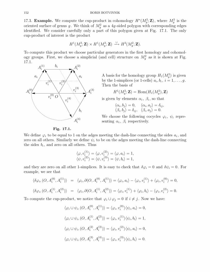
152 BORIS BOTVINNIK
17.3. Example. We compute the cup-product in cohomology H∗(M2g ;Z), where M2
g is theoriented surface of genus g . We think of M2
g as a 4g -sided polygon with corresponding edgesidentified. We consider carefully only a part of this polygon given at Fig. 17.1. The onlycup-product of interest is the product
H1(M2g ;Z)×H1(M2
g ;Z)∪−→ H2(M2
g ;Z).
To compute this product we choose particular generators in the first homology and cohomol-ogy groups. First, we choose a simplicial (and cell) structure on M2
g as it is shown at Fig.17.1.
ai
bi
bi
ai
O
A(0)i
A(1)i A
(2)i
A(3)i
A(4)i
v(0)i
v(1)i v
(2)i
v(3)i
v(4)i
Fig. 17.1.
A basis for the homology group H1(M2g ) is given
by the 1-simplices (or 1-cells) ai, bi , i = 1, . . . , g .Then the basis of
H1(M2g ;Z) = Hom(H1(M
2g ),Z)
is given by elements αi , βi , so that
〈αi, bj〉 = 0, 〈αi, aj〉 = δij,〈βi, bj〉 = δij , 〈βi, aj〉 = 0.
We choose the following cocycles ϕi , ψi repre-senting αi , βi respectively.
We define ϕi to be equal to 1 on the adges meeting the dash-line connecting the sides ai , andzero on all others. Similarly we define ψi to be on the adges meeting the dash-line connectingthe sides bi , and zero on all others. Thus
〈ϕ, v(1)i 〉 = 〈ϕ, v(2)
i 〉 = 〈ϕ, ai〉 = 1,
〈ψ, v(2)i 〉 = 〈ψ, v(3)
i 〉 = 〈ψ, bi〉 = 1,
and they are zero on all other 1-simplices. It is easy to check that δϕi = 0 and δψi = 0. Forexample, we see that
〈δϕi, (O,A(0)i , A
(1)i )〉 = 〈ϕi, ∂(O,A(0)
i , A(1)i )〉 = 〈ϕi, ai〉 − 〈ϕi, v(1)
i 〉+ 〈ϕi, v(0)i 〉 = 0,
〈δϕi, (O,A(1)i , A
(2)i )〉 = 〈ϕi, ∂(O,A(1)
i , A(2)i )〉 = 〈ϕi, v(1)
i 〉+ 〈ϕi, bi〉 − 〈ϕi, v(2)i 〉 = 0.
To compute the cup-product, we notice that ϕi ∪ ϕj = 0 if i 6= j . Now we have:
〈ϕi ∪ ψi, (O,A(0)i , A
(1)i )〉 = 〈ϕi, v(0)
i 〉〈ψi, ai〉 = 0,
〈ϕi ∪ ψi, (O,A(1)i , A
(2)i )〉 = 〈ϕi, v(1)
i 〉〈ψi, bi〉 = 1,
〈ϕi ∪ ψi, (O,A(2)i , A
(3)i )〉 = 〈ϕi, v(2)
i 〉〈ψi, ai〉 = 0,
〈ϕi ∪ ψi, (O,A(3)i , A
(4)i )〉 = 〈ϕi, v(3)
i 〉〈ψi, bi〉 = 0.
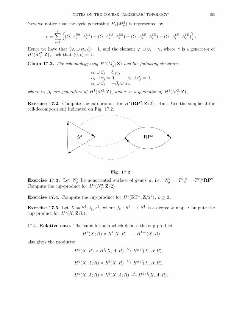
NOTES ON THE COURSE “ALGEBRAIC TOPOLOGY” 153
Now we notice that the cycle generating H2(M2g ) is represented by
c =
g∑
i=1
((O,A
(0)i , A
(1)i ) + (O,A
(1)i , A
(2)i ) + (O,A
(2)i , A
(3)i ) + (O,A
(3)i , A
(4)i )).
Hence we have that 〈ϕi ∪ ψi, c〉 = 1, and the element ϕi ∪ ψi = γ , where γ is a generator ofH2(M2
g ;Z), such that 〈γ, c〉 = 1.
Claim 17.2. The cohomology ring H∗(M2g ;Z) has the following structure:
αi ∪ βj = δijγ,αi ∪ αj = 0, βi ∪ βj = 0,αi ∪ βj = −βj ∪ αi.
where αi, βi are generators of H1(M2g ;Z), and γ is a generator of H2(M2
g ;Z),
Exercise 17.2. Compute the cup-product for H∗(RP2;Z/2). Hint: Use the simplicial (orcell-decomposition) indicated on Fig. 17.2.
∆2 RP2
Fig. 17.2.
Exercise 17.3. Let N2g be nonoriented surface of genus g , i.e. N2
g = T 2# · · ·T 2#RP2 .
Compute the cup-product for H∗(N2g ;Z/2).
Exercise 17.4. Compute the cup product for H∗(RP2;Z/2k), k ≥ 2.
Exercise 17.5. Let X = S1 ∪fke2 , where fk : S1 −→ S1 is a degree k map. Compute the
cup product for H∗(X;Z/k).
17.4. Relative case. The same formula which defines the cup product
Hk(X;R)×H l(X;R) −→ Hk+l(X;R)
also gives the products:
Hk(X;R)×H l(X,A;R)∪−→ Hk+l(X,A;R),
Hk(X,A;R)×H l(X;R)∪−→ Hk+l(X,A;R),
Hk(X,A;R)×H l(X,A;R)∪−→ Hk+l(X,A;R).

154 BORIS BOTVINNIK
Furthermore, if A, B are open in X or A, B are subcomplexes of a CW -complex X , thenthere is a more general cup relative product
Hk(X,A;R)×H l(X,B;R)∪−→ Hk+l(X,A ∪B;R).
We do not give details to define the last product. However we mention that the absolute cup
product Ck(X;R)× C l(X;R)∪−→ Ck+l(X;R) restricts to a cup product
Ck(X,A;R)× C l(X,B;R)∪−→ Ck+l(X,A +B;R),
where the group Cq(X,A + B;R) consits of cochains which vanish on chains in Cq(A) andin Cq(B). Then one should show that the inclusion map
Cq(X,A+B;R) −→ Cq(X,A ∪B;R)
induce isomorphism in cohomology groups, in a similar way as we did proving the ExcisionTheorem and Mayer-Vietoris Theorem.
Exercise 17.6. Prove that the cup product is natural, i.e. if f : X −→ Y is a map, andf ∗ : H∗(Y ;R) −→ H∗(X;R) is the induced homomorphism, then
f ∗(a ∪ b) = f ∗(a) ∪ f ∗(b).
17.5. External cup product. We define an external cup product
µ : H∗(X1;R)⊗R H∗(X2;R) −→ H∗(X1 ×X2;R)
as follows. Let pi : X1 ×X2 −→ Xi (i = 1, 2) be the projection onto Xi , i.e. pi(x1, x2) = xi .Then µ(a⊗ b) = p∗1(a)∪p∗2(b). The above tensor product ⊗R is taken over the ring R , whereH∗(Xi;R) are considered as R-modules. The tensor product H∗(X1;R) ⊗R H∗(X2;R) hasnatural multiplication defined as
(a1 ⊗ a2) · (b1 ⊗ b2) = (−1)deg b1 deg a2(a1b1 ⊗ a2b2).
Claim 17.3. The external product H∗(X1;R) ⊗R H∗(X2;R)µ−→ H∗(X1 × X2;R) is a ring
homomorphism.
Proof. Indeed, we have:
µ((a1 ⊗ a2) · (b1 ⊗ b2)) = µ((−1)deg b1 deg a2(a1b1 ⊗ a2b2))
= (−1)deg b1 deg a2p∗1(a1 ∪ b1) ∪ p∗2(a2 ∪ b2)
= (−1)deg b1 deg a2p∗1(a1) ∪ p∗1(b1) ∪ p∗2(a2) ∪ p∗2(b2)
= p∗1(a1) ∪ p∗2(a2) ∪ p∗1(b1) ∪ p∗2(b2)
= µ(a1 ⊗ a2)µ(b1 ⊗ b2).There are many important cases when the external product µ is an isomorphism, for examplefor X1 = Sk1 , and X2 = Sk2 .
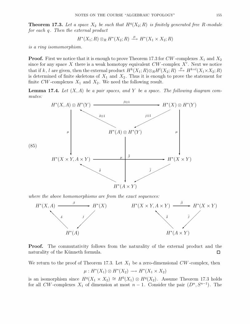
NOTES ON THE COURSE “ALGEBRAIC TOPOLOGY” 155
Theorem 17.3. Let a space X2 be such that Hq(X2;R) is finitely generated free R-modulefor each q . Then the external product
H∗(X1;R)⊗R H∗(X2;R)µ−→ H∗(X1 ×X2;R)
is a ring isomomorphism.
Proof. First we notice that it is enough to prove Theorem 17.3 for CW -complexes X1 and X2
since for any space X there is a weak homotopy equivalent CW -complex X ′ . Next we notice
that if k , l are given, then the external product Hk(X1;R)⊗RH l(X2;R)µ−→ Hk+l(X1×X2;R)
is determined of finite skeletons of X1 and X2 . Thus it is enough to prove the statement forfinite CW -complexes X1 and X2 . We need the following result.
Lemma 17.4. Let (X,A) be a pair spaces, and Y be a space. The following diagram com-mutes:
(85)
H∗(X,A)⊗H∗(Y )
?
µ
H∗(X)⊗H∗(Y )
j⊗1
?
µ
-β⊗1
H∗(A)⊗H∗(Y )HHHHHHHHHY
δ⊗1
?
µH∗(X × Y,A× Y ) H∗(X × Y )
j
-β
H∗(A× Y )HHHHHHHHHY
δ
where the above homomorphisms are from the exact sequences:
H∗(X,A) H∗(X)
j
-β
H∗(A)@
@@
@@Iδ
H∗(X × Y,A× Y ) H∗(X × Y )
j
-β
H∗(A× Y )@
@@
@@Iδ
Proof. The commutativity follows from the naturality of the external product and thenaturality of the Kunneth formula.
We return to the proof of Theorem 17.3. Let X1 be a zero-dimensional CW -complex, then
µ : H∗(X1)⊗H∗(X2) −→ H∗(X1 ×X2)
is an isomorphism since Hq(X1 × X2) ∼= H0(X1) ⊗ Hq(X2). Assume Theorem 17.3 holdsfor all CW -complexes X1 of dimension at most n − 1. Consider the pair (Dn, Sn−1). The
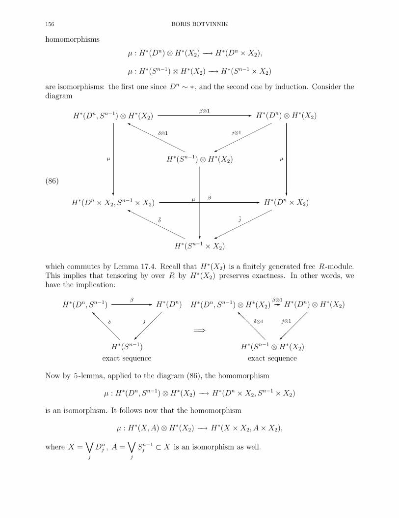
156 BORIS BOTVINNIK
homomorphisms
µ : H∗(Dn)⊗H∗(X2) −→ H∗(Dn ×X2),
µ : H∗(Sn−1)⊗H∗(X2) −→ H∗(Sn−1 ×X2)
are isomorphisms: the first one since Dn ∼ ∗ , and the second one by induction. Consider thediagram
(86)
H∗(Dn, Sn−1)⊗H∗(X2)
?
µ
H∗(Dn)⊗H∗(X2)
j⊗1
?
µ
-β⊗1
H∗(Sn−1)⊗H∗(X2)HHHHHHHHHY
δ⊗1
?
µH∗(Dn ×X2, S
n−1 ×X2) H∗(Dn ×X2)
j
-β
H∗(Sn−1 ×X2)HHHHHHHHHY
δ
which commutes by Lemma 17.4. Recall that H∗(X2) is a finitely generated free R-module.This implies that tensoring by over R by H∗(X2) preserves exactness. In other words, wehave the implication:
H∗(Dn, Sn−1) H∗(Dn)
j
-β
H∗(Sn−1)@
@@
@@Iδ
exact sequence
=⇒
H∗(Dn, Sn−1)⊗H∗(X2) H∗(Dn)⊗H∗(X2)
j⊗1
-β⊗1
H∗(Sn−1 ⊗H∗(X2)@
@@
@@Iδ⊗1
exact sequence
Now by 5-lemma, applied to the diagram (86), the homomorphism
µ : H∗(Dn, Sn−1)⊗H∗(X2) −→ H∗(Dn ×X2, Sn−1 ×X2)
is an isomorphism. It follows now that the homomorphism
µ : H∗(X,A)⊗H∗(X2) −→ H∗(X ×X2, A×X2),
where X =∨
j
Dnj , A =
∨
j
Sn−1j ⊂ X is an isomorphism as well.
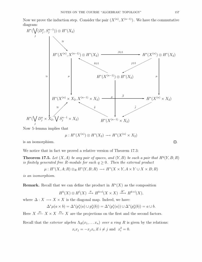
NOTES ON THE COURSE “ALGEBRAIC TOPOLOGY” 157
Now we prove the induction step. Consider the pair (X(n), X(n−1)). We have the commutativediagram:
H∗(∨
j
(Dnj , S
n−1j ))⊗H∗(X2)
@@
@@@R
∼=
?
∼=
H∗(X(n), X(n−1))⊗H∗(X2)
?
µ
H∗(X(n))⊗H∗(X2)
j⊗1
?
µ
-β⊗1
H∗(X(n−1))⊗H∗(X2)
HHHHHHHHHYδ⊗1
?
µH∗(X(n) ×X2, X
(n−1) ×X2) H∗(X(n) ×X2)
j
-β
H∗(∨
j
Dnj ×X2,
∨Sn−1j ×X2)
∼=
H∗(X(n−1) ×X2)
HHHHHHHHHYδ
Now 5-lemma implies that
µ : H∗(X(n))⊗H∗(X2) −→ H∗(X(n) ×X2)
is an isomorphism. .
We notice that in fact we proved a relative version of Theorem 17.3:
Theorem 17.5. Let (X,A) be any pair of spaces, and (Y,B) be such a pair that Hq(Y,B;R)is finitely generated free R-module for each q ≥ 0. Then the external product
µ : H∗(X,A;R)⊗R H∗(Y,B;R) −→ H∗(X × Y,A× Y ∪X × B;R)
is an isomorphism.
Remark. Recall that we can define the product in H∗(X) as the composition
Hk(X)⊗H l(X)µ−→ Hk+l(X ×X)
∆∗
−−→ Hk+l(X),
where ∆ : X −→ X ×X is the diagonal map. Indeed, we have:
∆∗µ(a× b) = ∆∗(p∗1(a) ∪ p∗2(b)) = ∆∗(p∗1(a)) ∪∆∗(p∗2(b)) = a ∪ b.Here X
p1←− X ×X p2−→ X are the projections on the first and the second factors.
Recall that the exterior algebra ΛR(x1, . . . xn) over a ring R is given by the relations:
xixj = −xjxi, if i 6= j and x2i = 0.

158 BORIS BOTVINNIK
Corollary 17.6. Let X = S2ℓ1+1 × · · · × S2ℓt+1 × S2k1 × · · · × S2ks . Then
H∗(X;R) ∼= ΛR(x2ℓ1+1, . . . , x2ℓt+1)⊗R[x2k1 , . . . , x2ks]/x2
2k1, . . . , x2
2ks,
where deg x2ℓi+1 = 2li + 1, deg x2kj= 2kj .
Example. Here is an important application of Theorem 17.5. We consider the pairs (X,A) =(Dk, Sk−1) and (Y,B) = (Dℓ, Sℓ−1). Then clearly the pair (Dℓ, Sℓ−1) satisfies the conditionsof Theorem 17.5. Thus we have a ring isomorphism
H∗(Dk, Sk−1;R)⊗R H∗(Dℓ, Sℓ−1;R) ∼= H∗(Dk ×Dℓ, Sk−1 ×Dℓ ∪ (−1)kDk × Sℓ−1;R)
∼= H∗(Dk+ℓ, Sk+ℓ−1;R)
since Sk−1 ×Dℓ ∪ (−1)kDk × Sℓ−1 ∼= Sk+ℓ−1 .
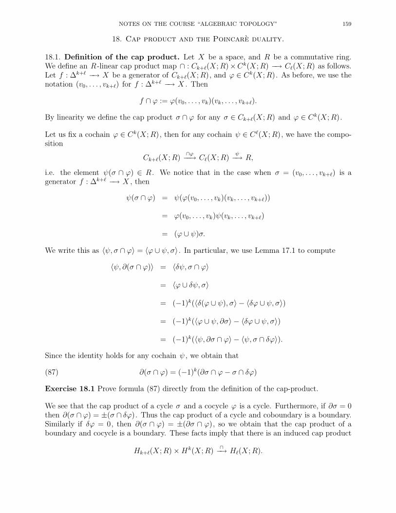
NOTES ON THE COURSE “ALGEBRAIC TOPOLOGY” 159
18. Cap product and the Poincare duality.
18.1. Definition of the cap product. Let X be a space, and R be a commutative ring.We define an R-linear cap product map ∩ : Ck+ℓ(X;R)×Ck(X;R) −→ Cℓ(X;R) as follows.Let f : ∆k+ℓ −→ X be a generator of Ck+ℓ(X;R), and ϕ ∈ Ck(X;R). As before, we use thenotation (v0, . . . , vk+ℓ) for f : ∆k+ℓ −→ X . Then
f ∩ ϕ := ϕ(v0, . . . , vk)(vk, . . . , vk+ℓ).
By linearity we define the cap product σ ∩ ϕ for any σ ∈ Ck+ℓ(X;R) and ϕ ∈ Ck(X;R).
Let us fix a cochain ϕ ∈ Ck(X;R), then for any cochain ψ ∈ Cℓ(X;R), we have the compo-sition
Ck+ℓ(X;R)∩ϕ−−→ Cℓ(X;R)
ψ−→ R,
i.e. the element ψ(σ ∩ ϕ) ∈ R . We notice that in the case when σ = (v0, . . . , vk+ℓ) is agenerator f : ∆k+ℓ −→ X , then
ψ(σ ∩ ϕ) = ψ(ϕ(v0, . . . , vk)(vk, . . . , vk+ℓ))
= ϕ(v0, . . . , vk)ψ(vk, . . . , vk+ℓ)
= (ϕ ∪ ψ)σ.
We write this as 〈ψ, σ ∩ ϕ〉 = 〈ϕ ∪ ψ, σ〉 . In particular, we use Lemma 17.1 to compute
〈ψ, ∂(σ ∩ ϕ)〉 = 〈δψ, σ ∩ ϕ〉
= 〈ϕ ∪ δψ, σ〉
= (−1)k(〈δ(ϕ ∪ ψ), σ〉 − 〈δϕ ∪ ψ, σ〉)
= (−1)k(〈ϕ ∪ ψ, ∂σ〉 − 〈δϕ ∪ ψ, σ〉)
= (−1)k(〈ψ, ∂σ ∩ ϕ〉 − 〈ψ, σ ∩ δϕ〉).
Since the identity holds for any cochain ψ , we obtain that
(87) ∂(σ ∩ ϕ) = (−1)k(∂σ ∩ ϕ− σ ∩ δϕ)
Exercise 18.1 Prove formula (87) directly from the definition of the cap-product.
We see that the cap product of a cycle σ and a cocycle ϕ is a cycle. Furthermore, if ∂σ = 0then ∂(σ ∩ ϕ) = ±(σ ∩ δϕ). Thus the cap product of a cycle and coboundary is a boundary.Similarly if δϕ = 0, then ∂(σ ∩ ϕ) = ±(∂σ ∩ ϕ), so we obtain that the cap product of aboundary and cocycle is a boundary. These facts imply that there is an induced cap product
Hk+ℓ(X;R)×Hk(X;R)∩−→ Hℓ(X;R).
160 BORIS BOTVINNIK
Using the same formulas one checks that the cap product has the relative form
Hk+ℓ(X,A;R)×Hk(X;R)∩−→ Hℓ(X,A;R),
Hk+ℓ(X,A;R)×Hk(X,A;R)∩−→ Hℓ(X;R),
Hk+ℓ(X,A ∪ B;R)×Hk(X,A;R)∩−→ Hℓ(X,B;R).
The last cap product is defined provided that A, B are open subsets of X or A, B aresubcomplexes of X (if X is a CW -complex).
Exercise 18.2 Check that the above relative cap products are well-defined.
Claim 18.1. Let f : X −→ Y be a map, and
f∗ : H∗(X;R) −→ H∗(Y ;R), f ∗ : H∗(Y ;R) −→ H∗(X;R)
be the induced homomorphisms. Then
f∗(σ ∩ f ∗(ϕ)) = f∗(σ) ∩ ϕ, σ ∈ H∗(X;R), ϕ ∈ H∗(Y ;R).
Exercise 18.3. Prove Claim 18.1.
Exercise 18.4. Let M2g be the oriented surface of the genus g . Let [M2
g ] ∈ H2(M2g ;Z) ∼= Z
be a generator. Define the homomorphism D : H1(M2g ;Z) −→ H1(M
2g ;Z) by the formula
D : α 7→ [M2g ] ∩ α . Compute the homomorphism D .
Exercise 18.5. Let N2g be the non-oriented surface of the genus g , i.e.
N2g = T 2# · · ·#T 2#RP2.
Let [N2g ] ∈ H2(N
2g ;Z/2) ∼= Z/2 be a generator. Define the homomorphism
D2 : H1(N2g ;Z/2) −→ H1(N
2g ;Z/2)
by the formula D2 : α 7→ [N2g ] ∩ α. Compute the homomorphism D2 .
Remark. The above homomorphism is the Poincare duality isomorphism specified for 2-dimensional manifolds.
18.2. Crash course on manifolds. Here I will be very brief and give only necessarydefinitions. A manifold is a second countable Hausdorff space M so that each pointx ∈ M has an open neighborhood U homeomorphic to Rn or a half-space Rn
+ =(x1, . . . , xn) ∈ Rn | xn ≥ 0. Then we say that dimM = n, and those point of M which donot have an open neighborhood homemorphic to Rn , form a boundary ∂M (which is alsoa closed manifold ∂M of dimension (n − 1)). We have seen some examples of manifolds:Rn , Sn , Dn (where ∂Dn = Sn−1 ), RPn , CPn , HPn , GLR(n), GLC(n), SO(n), U(n), allclassical Lie groups, Grassmannian, Stiefel manifolds and so on. To work with manifolds, weshould specify what do we mean by a smooth manifold.
NOTES ON THE COURSE “ALGEBRAIC TOPOLOGY” 161
Definition 18.1. An n-dimensional smooth manifold is a second countable Hausdorff spaceM together with a collection of charts, i.e. Uα of neighborhoods and homeomorphismsϕα → Rn (or ϕα → Rn
+ ) such that each point x ∈M is in some chart Uα , and if Uα∩Uα′ 6= ∅,then the map ϕα′ ϕ−1
α : ϕα(Uα ∩ Uα′)→ ϕα′(Uα ∩ Uα′) from the diagram
ϕα(Uα ∩ Uα′)
?
open subset
Uα ∩ Uα′ ϕα′(Uα ∩ Uα′)
?
open subset
-ϕ−1α -
ϕα′
Rn Rn
is a diffeomorphism.
All examples mentioned above are smooth manifolds. The following fact is very important inthe manifold theory.
Theorem 18.2. Any smooth manifold Mn is diffeomorphic to a submanifold of R2n , i.e.any manifold Mn can be embedded to a finite-dimensional Euclidian space.
Remark. I strongly recommend to read carefully few sections of Hatcher (Section 3.3-3.4)and Bredon (Sections II.1–II.4) to learn some basic facts and technique on smooth topology.
We recall that a subset X ⊂ Rk is triangulated (by q -simplices) if X is a union of simplicesX =
⋃i ∆
qi such that
• each simplex ∆qi is a nondegenerated simplex in Rk ;
• the intersection ∆qi ∩∆q
j is either empty or consists of is a single joint face of thesimplices ∆q
i and ∆qj .
Theorem 18.2 implies the following result we need to prove the Poincare duality.
Theorem 18.3. Any compact smooth manifold M of dimension n is homeomorphic to atriangulated (by n-simlpices) subset of a finitely-dimensional Euclidian space.
Remarks. (1) If dimM = n, then the Euclidian space in Theorem 18.3 could be chosento be R2n . Notice also that a triangulation of a manifold M induces a triangulation (bycorresponding (n− 1)-simplices) on its boundary ∂M .
(2) Theorem 18.3 holds also in the case when M is not compact. Then the triangulationshould be infinite.
(3) We do not prove Theorems 18.2, 18.3; say, Theorem 18.2 is rather easy to prove, andits proof could be found in most classical textbooks on Algebraic Topology; Theorem 18.3is deeper than it seems. First ad hock (and correct!) proof is due to Wittney (end of 30’s).A transperent version of that proof is given by Munkres in his “Lectures on DifferentialTopology”.
Exercise 18.6. Construct an embedding of the projective spaces RPn , CPn , HPn intoEuclidian space.
162 BORIS BOTVINNIK
Exercise 18.7. Let Mn ⊂ Rk be a triangulated (by n-simplices) manifold, M =⋃
∆ni ,
with possibly non-empty boundary ∂M . Consider any (n − 1)-face ∆n−1 of a simplex ∆ni .
Prove that if ∆n−1 does not belong to the induced triangulation of its boundary, then thereexists a unique simplex ∆n
j , j 6= i, which also has the simplex ∆n−1 as a face.
Consider the case when a manifold Mn ⊂ Rk is a compact closed (i.e. ∂Mn = ∅) manifold.Then we can assume that the triangulation Mn =
⋃i ∆
ni is finite. In particular, the trian-
gulation Mn =⋃i ∆
ni gives a CW -decomposition of the manifold M where n-cells eni are
identified with the enterior of the simplex ∆ni , and eni = ∆n
i . A triangulated manifold Mn issaid to be orientable (over a ring R) if there is a choice of orientations on each simplex ∆n
i ,such that the chain
(88)∑
i
eni (where the summation is taken over all indices i)
is a cycle in the chain complex E∗(M). Once we fix an orientations, we call the manifold Moriented.
Remark. If R = Z/2, then any closed compact manifold has “orientation”, and its unique.In that case one can see that the chain (88) is always a cycle.
We state the following result which summarizes our observations.
Theorem 18.4. Let Mn be a smooth compact manifold. Then
Hn(M ;Z) =
Z, if M is closed and oriented,0, else
Hn(M ;Z/2) =
Z/2, if M is closed,
0, else
Remarks. (1) It is easy to see that if a manifold Mn is oriented over Z, then it is orientedover any ring R . The converse is not true. It is also easy to see that any manifold Mn isoriented over Z/2 (Prove it!). A cohomology class defined by the cycle (88) is denoted by[Mn] ∈ Hn(M
n;R) and is called the fundamental class of Mn
(2) An example of a non-oriented manifold is RP2n : H2n(RP2n;Z) = 0; however, we havethe fundamental class [RP2n] ∈ H2n(RP2n;Z/2).
(3) We say that a homology class α ∈ Hk(Mn;R) is represented by a submanifold Nk ⊂ Mn
if i∗([Nk]) = α , where i : Nk → Mn is the inclusion map. For example, a generatorαk ∈ Hk(RPn) is represented by RPk ⊂ RPn ; as well as a generator βj ∈ H2j(CPn;Z) isrepresented by CPj ⊂ CPn . It turns out that not every homology class of a smooth manifoldcould be represented by a submanifold: this was discovered by Rene Thom in 1954.
18.3. Poincare isomorphism. Let Mn be a closed manifold. We define a homomorphism
D : Hq(M ;Z) −→ Hn−q(M ;Z) α 7→ [M ] ∩ α if M is oriented
D : Hq(M ;Z/2) −→ Hn−q(M ;Z/2) α 7→ [M ] ∩ α if M is not oriented

NOTES ON THE COURSE “ALGEBRAIC TOPOLOGY” 163
Theorem 18.5. (Poincare isomorphism Theorem) Let Mn be a closed compact manifold.Then the homorphism
D : Hq(M ;Z/2) −→ Hn−q(M ;Z/2)
is an isomorphism for each q . If, in addition, M is oriented manifold, then the homomor-phism
D : Hq(M ;Z) −→ Hn−q(M ;Z)
is an isomorphism for each q .
Remark. There are several different ways to prove Theorem 18.5. In particular, nice proofis given in the book by Hatcher (Sections 3.3-3.4). Here we will present a geometric proofwhich is rather close to an original idea due to Poincare.
Construction. Consider a triangulation T = ∆ni of an open disk Bn(r) ⊂ Rn of radius r .
Here it means that Bn(r) ⊂ ⋃i ∆ni , and the intersection ∆n
i ∩∆nj is either empty or consists
of is a single joint face of the simplices ∆ni and ∆n
j . We assume that the triangulation is fineenough, say, if ∆n
i ∩ Bn(r/2) 6= ∅ , then ∆ni ⊂ Bn(r). In other words, this triangulation is a
good local model of a neighborhood near a point on a manifold equipped with a triangulation.
Let ∆q ⊂ ∆ni ∈ T be a subsimplex with barycenter x0 at the center of the ball Bn(r). Now
let βT be the barycentric subdivision of our triangultion. We define a barycentric star S(∆q)as the following union (see Fig. 18.1):
S(∆q) :=⋃
∆ ⊂ ∆n ∈ βT∆ ∩∆q = x0
∆ .
Notice that all subsimplices ∆ with those properties have dimension (n − q), moreover,S(∆q) ⊂ Bn(r) is homeomorphic to a disk Dn−q decomposed into (n− q)-simplices, see Fig.18.2.
Proof of Theorem 18.5. Let T be a triangulation of a closed oriented manifold Mn . Inparticular, the triangulation T determines a CW -decomposition of Mn , where all q -cells aregiven by q -simplices ∆q
i of T . We notice that the stars S(∆q) determine an alternative“dual” CW -structure of Mn . Let E∗(Mn) be a chain complex determined by the first CW -decomposition, and E∗(Mn) the chain complex determined by the dual CW -structure.
In particular, generators of the chain group En−q(Mn) are the stars S(∆qi ). Also, let
E∗(Mn) = Hom(E∗(Mn),Z) be the corresponding cochain complex. We define a homomor-phism D : Eq(Mn) → En−q(Mn) as follows. For a cochain ϕ ∈ Eq(Mn), ϕ : ∆q
i 7→ λi , wedefine
D(ϕ) :=∑
i
λiS(∆qi ) ∈ En−q(Mn).

164 BORIS BOTVINNIK
Fig. 18.1. A barycentric star in Rn .
It is easy to check that Dδϕ = ±∂Dϕ (we do not specify the sign here). Thus we have thefollowing commutative diagram:
En(Mn) En−1(Mn) · · · E1(Mn) E0(Mn)-∂n -∂n−1 -∂2 -∂1
E0(Mn)
6
D
E1(Mn)
6
D
· · · En−1(Mn)
6
D
En(Mn)
6
D
-δ1 -δ2 -δn−2 -δn−1
Thus we have that D is an isomorphism for each q and, in fact, the above complexesE∗(Mn) and E∗(Mn) are identical via the chain map D . Hence we have that Hq(Mn;Z) ∼=Hn−q(Mn;Z).
Exercise 18.9. Show that the duality isomomorphism D induces the map as
D : Hq(Mn;Z)[Mn]∩−−−−→ Hn−q(M
n;Z).
Hint: replace the cochain complex E∗(Mn) by the the cochain complex given by the barycenticsubdivision βT .
This concludes our proof of Theorem 18.5.
Corollary 18.6. Let Mn be a closed compact manifold of odd dimension n. Then χ(Mn) =0.
Exercise 18.10. Prove Corollary 18.6. Notice that Mn is not necessarily an oriented mani-fold.

NOTES ON THE COURSE “ALGEBRAIC TOPOLOGY” 165
18.4. Some computations. Recall that for the cap-product
Hk+ℓ(X;R)×Hk(X;R)∩−→ Hℓ(X;R).
we have the identity 〈ψ, σ ∩ϕ〉 = 〈ϕ∪ψ, σ〉 . For a closed oriented manifold Mn we considerthe pairing
(89) Hq(Mn;R)×Hn−q(Mn;R)→ R, (ϕ, ψ) := 〈ϕ ∪ ψ, [Mn]〉.A bilinear pairing µ : A × B → R , (where A and B are R-modules) is nonsingular if themaps
A→ HomR(B,R), a 7→ µ(a, ·) ∈ HomR(B,R), and
B → HomR(A,R), b 7→ µ(·, b) ∈ HomR(A,R)
are both isomorphisms.
Lemma 18.7. Let Mn be an oriented manifold (over R). Then the pairing (89) is nonsin-gular provided that R is a field. Furthermore, if R = Z, then the induced pairing
(90) (Hq(Mn;Z)/Tor)×(Hn−q(Mn;Z)/Tor
)→ Z, (ϕ, ψ) := 〈ϕ ∪ ψ, [Mn]〉.
is nonsingular.
Exercise 18.11. Prove Lemma 18.7. Hint: Make use of the universal coefficient Theoremand Poincare duality.
Corollary 18.8. Let Mn be an oriented manifold. Then for each element of infinite orderα ∈ Hq(Mn;Z), there exists an element β ∈ Hn−q(Mn;Z) of infinite order such that 〈α ∪β, [Mn]〉 = 1, i.e. the element α ∪ β is a generator of the group Hn(Mn;Z).
Exercise 18.12. Prove Corollary 18.8.
Theorem 18.9. Let R be any ring. Then
(1) H∗(RPn;Z/2) ∼= Z/2[x]/xn+1 , where x ∈ H1(RPn;Z/2) is a generator;(2) H∗(CPn;R) ∼= R[y]/yn+1 , where y ∈ H2(CPn;R) is a generator;(3) H∗(HPn;R) ∼= R[z]/zn+1 , where z ∈ H4(HPn;R) is a generator.
Proof. We prove (2). Induction on n. Clearly H∗(CP1;R) ∼= R[y]/y2 . Induction step. Theinclusion i : CPn−1 → CPn induces an isomorphism
i∗ : Hq(CPn;Z)→ Hq(CPn−1;Z)
for q ≤ n− 1. In particular, the groups H2j(CPn−1;Z) are generated by yj for j ≤ n− 1.
By Corollary 18.7, there exists an integer m such that the element yn−1∪my = myn generatesthe group H2n(CPn−1;Z) ∼= Z. Thus we obtain that m = ±1, and H∗(CPn;R) ∼= R[y]/yn+1 .
Corollary 18.10. Let R be any ring. Then
(1) H∗(RP∞;Z/2) ∼= Z/2[x], where x ∈ H1(RPn;Z/2) is a generator;(2) H∗(CP∞;R) ∼= R[y], where y ∈ H2(CPn;R) is a generator;(3) H∗(HP∞;R) ∼= R[z], where z ∈ H4(HPn;R) is a generator.
166 BORIS BOTVINNIK
19. Hopf Invariant
19.1. Whitehead product. Here we remind the Whitehead product: for any elements α ∈πm(X), β ∈ πn(X) we construct the element [α, β] ∈ πm+n−1(X).
First we consider the product Sm × Sn . The cell structure of Sm × Sn is obvious: wehave cells σ0 , σm , σn , σm+n . A union of the cells σ0 , σm , σn is the space Sm ∨ Sn . Letw : Sm+n−1 −→ Sm ∨ Sn be an attaching map of the cell σm+n , i.e.
Sm × Sn = (Sm ∨ Sn) ∪w Dm+n−1.
Now let f : Sm −→ X , g : Sn −→ X be representatives of elements α ∈ πm(X), β ∈ πn(X).The composition
Sm+n−1 w−→ Sm ∨ Sn f∨g−−→ X
gives an element of πm+n−1(X). By definition,
[α, β] = the homotopy class of (f ∨ g) w .The construction above does depend on a choice of the attaching map w .
Let ι2n be a generator of the group π2n(S2n). We have proved “geometrically” the following
result.
Theorem 19.1. The group π4n−1(S2n) is infinite for any n ≥ 1; the element [ι2n, ι2n] ∈
π4n−1(S2n) has infinite order.
Next, we introduce an invariant, known as Hopf invariant to give another proof of Theorem19.1.
19.2. Hopf invariant. Before proving the theorem we define the Hopf invariant. Letϕ ∈ π4n−1(S
2n), and let f : S4n−1 −→ S2n be a representative of ϕ . Let Xϕ = S2n ∪f D4n .Compute the cohomology groups of Xϕ :
Hq(Xϕ;Z) =
Z, q = 0, 2n, 4n,0, otherwise.
Let a ∈ H2n(Xϕ;Z), b ∈ H4n(Xϕ;Z) be generators. Since a2 = a ∪ a ∈ H4n(Xϕ;Z), thena2 = hb, where h ∈ Z. The number h(ϕ) = h is the Hopf invariant of the elementϕ ∈ π4n−1(S
2n).
Examples. Let h : S3 → CP1 = S2 and H : S7 → HP1 = S4 be the Hopf maps. Noticethat Xh = CP2 and XH = HP2 . As we have computed,
H∗(CP2;Z) = Z[y]/y3, y ∈ H2(CP2;Z),
H∗(HP2;Z) = Z[z]/z3, z ∈ H4(HP4;Z).
Thus h(h) = 1 and h(H) = 1. There is one more case when this is true. Let Ca be theCalley algebra; this is the algebra defined on R8 . Furthermore, there exists a projective lineCaP1 ∼= S8 and a projective plane CaP2 with
H∗(CaP2;Z) = Z[σ]/σ3, σ ∈ H8(CaP2;Z).
The attaching map H : S15 → S8 for the cell e16 also has h(H) = 1.
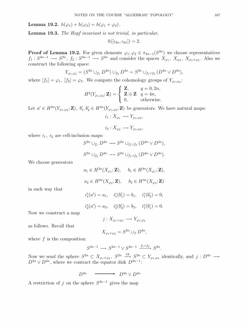
NOTES ON THE COURSE “ALGEBRAIC TOPOLOGY” 167
Lemma 19.2. h(ϕ1) + h(ϕ2) = h(ϕ1 + ϕ2).
Lemma 19.3. The Hopf invariant is not trivial, in particular,
h([ι2n, ι2n]) = 2.
Proof of Lemma 19.2. For given elements ϕ1, ϕ2 ∈ π4n−1(S2n) we choose representatives
f1 : S4n−1 −→ S2n , f2 : S4n−1 −→ S2n and consider the spaces Xϕ1 , Xϕ2 , Xϕ1+ϕ2 . Also weconstruct the following space:
Yϕ1,ϕ2 = (S2n ∪f1 D4n) ∪f2 D4n = S2n ∪f1∨f2 (D4n ∨D4n),
where [f1] = ϕ1 , [f2] = ϕ2 . We compute the cohomology groups of Yϕ1,ϕ2 :
Hq(Yϕ1,ϕ2;Z) =
Z, q = 0, 2n,Z⊕ Z q = 4n,0, otherwise.
Let a′ ∈ H2n(Yϕ1,ϕ2;Z), b′1, b′2 ∈ H4n(Yϕ1,ϕ2;Z) be generators. We have natural maps:
i1 : Xϕ1 −→ Yϕ1,ϕ2,
i2 : Xϕ2 −→ Yϕ1,ϕ2,
where i1 , i2 are cell-inclusion maps:
S2n ∪f1 D4n −→ S2n ∪f1∨f2 (D4n ∨D4n),
S2n ∪f2 D4n −→ S2n ∪f1∨f2 (D4n ∨D4n).
We choose generators
a1 ∈ H2n(Xϕ1 ;Z), b1 ∈ H4n(Xϕ1 ;Z),
a2 ∈ H2n(Xϕ2;Z), b2 ∈ H4n(Xϕ2;Z)
in such way thati∗1(a
′) = a1, i∗1(b′1) = b1, i∗1(b
′2) = 0,
i∗2(a′) = a2, i∗2(b
′2) = b2, i∗1(b
′1) = 0.
Now we construct a mapj : Xϕ1+ϕ2 −→ Yϕ1,ϕ2
as follows. Recall thatXϕ1+ϕ2 = S2n ∪f D4n,
where f is the composition:
S4n−1 −→ S4n−1 ∨ S4n−1 f1∨f2−−−→ S2n.
Now we send the sphere S2n ⊂ Xϕ1+ϕ2 , S2n Id−→ S2n ⊂ Yϕ1,ϕ2 identically, and j : D4n −→D4n ∨D4n , where we contract the equator disk D4n−1 :
D4n - D4n ∨D4n
A restriction of j on the sphere S4n−1 gives the map
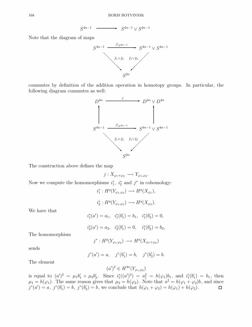
168 BORIS BOTVINNIK
S4n−1 - S4n−1 ∨ S4n−1
Note that the diagram of maps
S4n−1
@@
@@@R
f1+f2
S4n−1 ∨ S4n−1
f1∨f2
-j|
S4n−1
S2n
commutes by definition of the addition operation in homotopy groups. In particular, thefollowing diagram commutes as well:
D4n D4n ∨D4n-j
S4n−1
@@
@@@R
f1+f2
6
S4n−1 ∨ S4n−1
f1∨f2
6
-j|
S4n−1
S2n
The construction above defines the map
j : Xϕ1+ϕ2 −→ Yϕ1,ϕ2 .
Now we compute the homomorphisms i∗1 , i∗2 and j∗ in cohomology:
i∗1 : Hq(Yϕ1,ϕ2) −→ Hq(Xϕ1),
i∗2 : Hq(Yϕ1,ϕ2) −→ Hq(Xϕ2).
We have thati∗1(a
′) = a1, i∗1(b′1) = b1, i∗1(b
′2) = 0,
i∗2(a′) = a2, i∗2(b
′1) = 0, i∗1(b
′2) = b2,
The homomorphism
j∗ : Hq(Yϕ1,ϕ2) −→ Hq(Xϕ1+ϕ2)
sends
j∗(a′) = a, j∗(b′1) = b, j∗(b′2) = b.
The element
(a′)2 ∈ H4n(Yϕ1,ϕ2)
is equal to (a′)2 = µ1b′1 + µ2b
′2 . Since i∗1((a
′)2) = a21 = h(ϕ1)b1 , and i∗1(b
′1) = b1 , then
µ1 = h(ϕ1). The same reason gives that µ2 = h(ϕ2). Note that a2 = h(ϕ1 + ϕ2)b, and sincej∗(a′) = a, j∗(b′1) = b, j∗(b′2) = b, we conclude that h(ϕ1 + ϕ2) = h(ϕ1) + h(ϕ2).
NOTES ON THE COURSE “ALGEBRAIC TOPOLOGY” 169
Before we prove Lemma 19.3, we compute the cohomology (together with a product structure)Hq(S2n × S2n). First compute the cohomology groups:
Hq(S2n × S2n;Z) =
Z, q = 0, 4n,Z⊕ Z, q = 2n
0, otherwise.
Let c1, c2 ∈ H2n(S2n × S2n) be such generators that the homomorphisms
p∗1 : H2n(S2n1 ) −→ H2n(S2n
1 × S2n2 ),
p∗2 : H2n(S2n2 ) −→ H2n(S2n
1 × S2n2 ),
induced by the projections
S2n1 × S2n
2
p1−→ S2n1 , S2n
1 × S2n2
p2−→ S2n2
send the generators c1 and c2 to the generators of the groups H2n(S2n1 ), H2n(S2n
2 ). Letd ∈ H4n(S2n × S2n) be a generator. It follows from Corollary 17.6 that
c1c2 = d.
We also note that c21 = 0 and c22 = 0 since by naturality p∗1(c1)2 = 0 and p∗2(c2)
2 = 0. Sowe have that the ring H∗(S2n
1 × S2n2 ) is generated over Z by the elements 1, c1 , c2 with the
relations c21 = 0, c22 = 0. In particular, we have:
(c1 + c2)2 = c21 + 2c1c2 + c22 = 2d.
Proof of Lemma 19.3. We consider the factor space
X = S2n × S2n/ ∼,where we identify the points (x, x0) = (x0, x), where x0 is the base point of S2n .
Claim 19.1. The space X = S2n× S2n/ ∼ is homeomorphic to the space S2n ∪f D4n , wheref is the map defining the Whitehead product [ι2n, ι2n].
Proof of Claim 19.1. Recall that S2n× S2n = (S2n ∨ S2n)∪w D4n , where w is the map wedescribed above. The generator ι2n is represented by the identical map S2n −→ S2n . Thecomposition
S4n−1 w−→ S2n ∨ S2n Id∨Id−−−→ S2n
represents the element [ι2n, ι2n]. It exatly means that the identification (S2n, x0) = (x0, S2n)
we just did in the space S2n × S2n is the same as to attach D4n with the attaching map(Id ∨ Id) w .
Compute the cohomology of X :
Hq(X;Z) =
Z, q = 0, 2n, 4n,0, otherwise.
We note that the projection S2n × S2n −→ X sends the generator c ∈ H2n(X) to c1 + c2 .Besides the generator d maps to a generator of H4n(X;Z) (we denote it also by d). So wehave: c2 = 2d , or h([ι2n, ι2n]) = 2.
This concludes our proof of Theorem 19.1.

170 BORIS BOTVINNIK
Remarks. (1) In fact, it is true that π4n−1(S2n) = Z⊕finite abelian group , in particular,
as we know, π3(S2) = Z, π7(S
4) = Z ⊕ Z/12, π11(S6) = Z, π15(S
8) = Z ⊕ Z/120. More-over, all homotopy groups of the spheres are finite with the exception of πn(S
n) = Z andπ4n−1(S
2n) = Z⊕ finite abelian group .
(2) We proved that the image of the Hopf invariant h : π4n−1(S2n) −→ Z either all group Z
or 2Z.
Problem: Does there exists an element in π4n−1(S2n) with the Hopf invariant 1?
This problem has several remarkable reformulations. One of them is the following: for whichn does the vector space Rn+1 admit a structure of real division algebra with a unit. FrankAdams (1960) proved that there are elements with the Hopf invariant one only in the groupsπ3(S
2) π6(S4), π15(S
8). Thus there are only the following real division algebra with a unit:R2 ∼= C, R4 ∼= H , and R8 ∼= Ca.

NOTES ON THE COURSE “ALGEBRAIC TOPOLOGY” 171
20. Elementary obstruction theory
20.1. Eilenberg-MacLane spaces and cohomology operations. Let π and G be abeliangroups, n, m be nonnegtive integers.
Definition 20.1. A family of maps
θX : Hn(X; π)→ Hn′
(X; π′)
is called a cohomology operation θ of the type (π, n; π′, n′) if it is determined for every topo-logical space X and such that for any map f : X → Y the diagram
Hn(X; π) Hn′
(X; π′)-θX
Hn(Y ; π)
6f∗
Hn′
(Y ; π′)
6f∗
-θY
commutes, i.e. f ∗θY = θXf∗ . In different terms, we say that the operation θ is natural. The
set of all cohomological operations of the type (π, n; π′, n′) is denoted by O(π, n; π′, n′).
Example. For each n and any π the operation a 7→ a2 is a cohomology operation. Noticethat a cohomology operation is not, in general, a homomorphism.
Our next goal is to idendify the set O(π, n; π′, n′) with cohomology groups of the Eilenberg-McLane spaces.
Let X be a space. We recall that there is Hurewicz homomorphism h : πq(X) → Hq(X;Z)defined as follows. Let ιq ∈ Hq(S
q) be a canonical generator. Then for an element ϕ ∈ πq(X)and its represenative f : Sq → X , the image h(ϕ) ∈ Hq(X;Z) is given by f∗(ιq).
Now assume that X is (n−1)-connected. Then Hq(X;Z) = 0 for q ≤ n−1 and the Hurewiczhomomorphism h : πn(X) → Hn(X;Z) is isomorphism. Then the universal coefficient for-mula
0→ Ext(Hn−1(X;Z), π)→ Hn(X; π)→ Hom(Hn(X;Z), π)→ 0
shows that Hn(X; π) ∼= Hom(Hn(X;Z), π) since Hn−1(X;Z) = 0.
Let π = πn(X). Thus the group Hom(Hn(X;Z), π) contains the inverse h−1 to the Hurewiczhomomorphism h.
Definition 20.2. For an (n− 1)-connected space X , we denote by ιX the cohomology class
ιX := h−1 ∈ Hom(Hn(X;Z), π) ∼= Hn(X; π).
Sometimes the class ιX is called as fundamental class of (n− 1)-connected space X .
In particular, the Eilenberg-McLane space K(π, n) has a canonical class
ιn ∈ Hom(Hn(K(π, n);Z), π).
Below we will prove the following result.
172 BORIS BOTVINNIK
Theorem 20.3. There is a bijection
[X,K(π, n)]↔ Hn(X; π).
given by the formula [f ] 7→ f ∗ιn .
Here [f ] means a homotopy class of a map f : X → K(π, n). Before proving Theorem 20.3,we derive several important corollaries of Theorem 20.3.
Corollary 20.4. Let π , π′ be abelian groups. There is a bijection
[K(π, n), K(π′, n)]↔ Hom(π, π′).
Proof. We combine the statement of Theorem 20.3 with the universal coefficient theoremand Hurewicz isomorphism to see that
[K(π, n), K(π′, n)]↔ Hn(K(π, n); π′) ∼= Hom(Hn(K(π, n);Z), π′) ∼= Hom(π, π′).
This proves Corollary 20.4.
Corollary 20.5. Let π be an abelian group. The homotopy type of the Eilenberg-McLanespace K(π, n) is completely determined by the group π and the integer n.
Proof. According to Corollary 20.4, any isomorphism π → π is induced by some map f :K(π, n)→ K(π, n). Since all other groups are trivial, the map f induces isomorphism in allhomotopy groups. Then Whitehead Theorem 14.10 implies that f is homotopy equivalence.
Now let θ be a cohomology operation of the type (π, n; π′, n′). Then we have en elementθ(ιn) ∈ Hn′
(K(π, n), π′).
Theorem 20.6. There is a bijection
O(π, n; π′, n′)↔ Hn′
(K(π, n), π′)
given by the formula θ ↔ θ(ιn).
Proof. Let ϕ ∈ Hn′
(K(π, n), π′). We define an operation ϕ ∈ O(π, n; π′, n′) as follows. Weshould describe the action
Hn(X; π)ϕX−−→ Hn′
(X; π′)
for any space X . Let u ∈ Hn(X; π), then, according to Theorem 20.3, there exists a mapf : X → K(π;n) such that [f ] 7→ f ∗(ιn) = u . Then we define
ϕ(u) = f ∗(ϕ) ∈ Hn′
(X; π′).
Thus we have the maps
O(π, n; π′, n′)→ Hn′
(K(π, n), π′), ϕ 7→ ϕ(ιn)
Hn′
(K(π, n), π′)→ O(π, n; π′, n′), ϕ(u) = f ∗(ϕ), where f ∗(ιn) = u.
Let X = K(π, n) and u = ιn , then f : K(π, n) → K(π, n) is homotopic the identity. Thusϕ(ιn) = f ∗(ϕ) = ϕ . In the other direction, let ϕ = θ(ιn). Then
ϕ(u) = f ∗(ϕ) = f ∗(θ(ιn)) = θ(f ∗(ιn)) = θ(u)
for any u ∈ Hn(X; π).
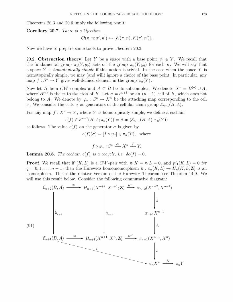
NOTES ON THE COURSE “ALGEBRAIC TOPOLOGY” 173
Theorems 20.3 and 20.6 imply the following result:
Corollary 20.7. There is a bijection
O(π, n; π′, n′)↔ [K(π, n), K(π′, n′)].
Now we have to prepare some tools to prove Theorem 20.3.
20.2. Obstruction theory. Let Y be a space with a base point y0 ∈ Y . We recall thatthe fundamental group π1(Y, y0) acts on the group πn(Y, y0) for each n. We will say thata space Y is homotopically simple if this action is trivial. In the case when the space Y ishomotopically simple, we may (and will) ignore a choice of the base point. In particular, anymap f : Sn → Y gives well-defined element in the group πn(Y ).
Now let B be a CW -complex and A ⊂ B be its subcomplex. We denote Xn = B(n) ∪ A,where B(n) is the n-th skeleton of B . Let σ = en+1 be an (n+ 1)-cell of B , which does notbelong to A. We denote by ϕσ : Sn → Xn be the attaching map corresponding to the cellσ . We consider the cells σ as generators of the cellular chain group En+1(B,A).
For any map f : Xn → Y , where Y is homotopically simple, we define a cochain
c(f) ∈ En+1(B,A; πn(Y )) = Hom(En+1(B,A), πn(Y ))
as follows. The value c(f) on the generator σ is given by
c(f)(σ) = [f ϕσ] ∈ πn(Y ), where
f ϕσ : Snϕσ−→ Xn f−→ Y.
Lemma 20.8. The cochain c(f) is a cocycle, i.e. δc(f) = 0.
Proof. We recall that if (K,L) is a CW -pair with π1K = π1L = 0, and pi1(K,L) = 0 forq = 0, 1, . . . , n − 1, then the Hurewicz homomomorphism h : πn(K,L) → Hn(K,L;Z) is anisomorphism. This is the relative version of the Hurewicz Theorem, see Theorem 14.9. Wewill use this result below. Consider the following commutative diagram:
(91)
XXXXXXXXXXXXXXXXXXXXXXXXz
i
En+2(B,A)
?
∂≀
n+2
Hn+2(Xn+2, Xn+1;Z)
?
∂≀
n+2
πn+2(Xn+2, Xn+1)
?
∂
-∼= -h
−1
πn+1Xn+1
?
j∗
En+1(B,A) Hn+1(Xn+1, Xn;Z) πn+1(X
n+1, Xn)
?
∂
-∼= -h−1
πnXn πnY-f∗
174 BORIS BOTVINNIK
Here the horizontal homomorphisms are given by the inverses to the Hurewicz isomorphisms.By definition, the boundary operator
∂≀
n+2 : Hn+2(Xn+2, Xn+1;Z) −→ Hn+1(X
n+1, Xn;Z)
is given by the boundary operator in the long exact sequence of the triple (Xn+2, Xn+1, Xn)and thus by Hurewicz isomorphism is reduced to the boundary operator in the long exactsequence in homotopies for the same triple:
∂ : πn+2(Xn+2, Xn+1) −→ πn+1(X
n+1, Xn)
which coincides with the composition:
πn+2(Xn+2, Xn+1)
∂−→ πn+1Xn+1 j∗−→ πn+1(X
n+1, Xn).
by construction. Here ∂ is the boundary operator in the long exact sequence in homotopygroups for the pair (Xn+2, Xn+1). Then we identify the cochain c(f) : En+1(B,A) → πnY ;clearly it coinsides with the composition f∗ i. Now let σ ∈ En+2(B,A). By definition,
δn+1c(f)(σ) = c(f)(∂≀
n+2σ). On the other hand, we can first take σ to σ ∈ πn+2(Xn+2, Xn+1)
via the Hurewicz isomorphism and then down the right column of the diagram (91). Then
we have ∂ f∗ ∂(σ) = 0 since ∂ f∗ = 0 by exactness.
Exercise 20.1. Prove the following Lemma 20.9.
Lemma 20.9. The map f : Xn → Y can be extended to a map f : Xn+1 → Y if and only ifc(f) = 0.
Now let f, g : Xn → Y be two maps which coincide on Xn−1 , i.e. f |Xn−1 = g|Xn−1 . Thenfor each n-cell ω , we define a map hω : Sn → Y as follows. We decompose Sn as union ofthe hemispheres: Sn = Dn
+ ∪Sn−1 Dn− . Then for each n-cell ω , we have the attaching map
ψω : Sn−1 → Xn−1 = B(n−1) ∪ A and characteristic map Ψω : Dn → Xn = B(n) ∪ A. Thenwe define hω : Sn = Dn
+ ∪Sn−1 Dn− → Y by
hω|Dn+
= g Ψω : Dn+
Ψω−→ Xn g−→ Y,
hω|Dn−
= f Ψω : Dn−
Ψω−→ Xn f−→ Y.
Clearly hω|Sn−1 = (f Ψω)|Sn−1 = (g Ψω)|Sn−1 since f |Xn−1 = g|Xn−1 . This constructiondefines the distinguishing cochain d(f, g) in the cochain group En(B,A; πn(Y )).
Lemma 20.10. There are the following properties of the cochain d(f, g):
(1) Let f, g : Xn → Y be two maps which coincide on Xn−1 , then
δd(f, g) = c(g)− c(f).
(2) Let f, g, h : Xn → Y be three maps which coincide on Xn−1 , then
d(f, g) + d(g, h) = d(f, h).
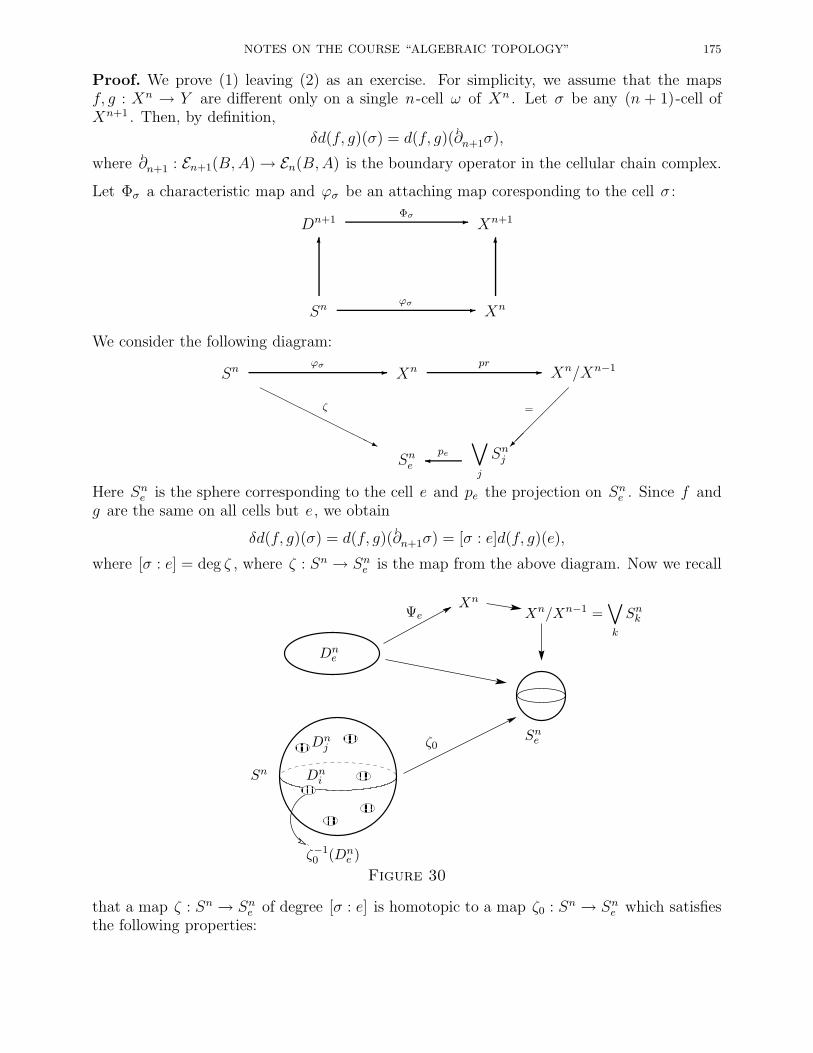
NOTES ON THE COURSE “ALGEBRAIC TOPOLOGY” 175
Proof. We prove (1) leaving (2) as an exercise. For simplicity, we assume that the mapsf, g : Xn → Y are different only on a single n-cell ω of Xn . Let σ be any (n + 1)-cell ofXn+1 . Then, by definition,
δd(f, g)(σ) = d(f, g)(∂≀
n+1σ),
where ∂≀
n+1 : En+1(B,A)→ En(B,A) is the boundary operator in the cellular chain complex.
Let Φσ a characteristic map and ϕσ be an attaching map coresponding to the cell σ :
Dn+1 Xn+1-Φσ
Sn
6
Xn
6
-ϕσ
We consider the following diagram:
Sn
HHHHHHHHHj
ζ
Xn Xn/Xn−1
=
-ϕσ -pr
Sne
∨
j
Snjpe
Here Sne is the sphere corresponding to the cell e and pe the projection on Sne . Since f andg are the same on all cells but e, we obtain
δd(f, g)(σ) = d(f, g)(∂≀
n+1σ) = [σ : e]d(f, g)(e),
where [σ : e] = deg ζ , where ζ : Sn → Sne is the map from the above diagram. Now we recall
Sn
ζ0
ζ−10 (Dn
e )
Dnj
Dni
Dne
ΨeXn
Xn/Xn−1 =∨
k
Snk
Sne
Figure 30
that a map ζ : Sn → Sne of degree [σ : e] is homotopic to a map ζ0 : Sn → Sne which satisfiesthe following properties:
176 BORIS BOTVINNIK
(1) there are disjoint disks Dn1 , . . . , D
ns ⊂ Sn such that
(a) ζ0|Dnj
: Dnj → Sne is a map of degree ±1;
(b) ζ0|Sn\(Dn1 ⊔...⊔Dn
s ) : Sn \ (Dn1 ⊔ . . . ⊔Dn
s )→ Sne is a constant map;
(2) the degree [σ : e] is the algebraic number of such disks counting ±1’s.
Now we can take a close look at the cell en ⊂ Xn , see Fig. 30. It shows that
(c(f)− c(g))(σ) = [σ : e]d(f, g)(e)
This proves the result.
It turns out that any cochain in En(B,A; πn(Y )) could be realized as a distinguishing cochain:
Lemma 20.11. For any map f : Xn → Y and a cochain d ∈ En(B,A; πn(Y )) there exists amap g : Xn → Y such that f |Xn−1 = g|Xn−1 and d(f, g) = d.
Exercise 20.2. Prove Lemma 20.11.
We denote by [c(f)] ∈ Hn+1(B,A; πnY ) the cohomology class of c(f).
Theorem 20.12. Let Y be a homotopy simple space, (B,A) a CW -pair and Xn = B(n)∪Afor n = 0, 1, . . .. Assume f : Xn −→ Y is a map. Then there exists a map g : Xn+1 −→ Ysuch that g|Xn−1 = f |Xn−1 if and only if [c(f)] = 0 in Hn+1(B,A; πnY ).
Proof. Let δd = c(f). Then we find g : Xn −→ Y such that g|Xn−1 = f |Xn−1 and d(f, g) =−d . Since
c(f) = δd = −δd(f, g) = c(f)− c(g),we obtain that c(g) = 0. Thus there exists an extension of g to Xn+1 .
Let K be a CW -complex. Then we let B = K × I , A = K × 0, 1. To illustrate thetechnique, we give another proof of the following simple fact.
Lemma 20.13. Let Y be n-connected space and K be a CW -complex of dimension n. Then[K, Y ] = ∗.
Proof. Let h : K → Y be a map. We define a map f : K × 0, 1 → Y as
f |K×0 = h, f |K×1 = ∗We choose a CW -structure of K × I to be a product-structure. In particular, all zero cellsof K × I are located inside of K × 0, 1. Thus the map
f (0) : X0 = (K × I)(0) ∪K × 0, 1 → Y
is already defined. Assume that its exension
f (k) : Xk = (K × I)(k) ∪K × 0, 1 → Y
to the space Xk = (K × I)(k) ∪K ×0, 1 for k = 0, . . . , ℓ− 1 is defined, where ℓ ≤ n. Thenthe obstruction c(f (ℓ)) ∈ E ℓ(K × I,K × 0, 1 ; πℓ(Y )) vanishes since πℓ(Y ) = 0. This showsthat a homotopy between h and the constant map extends to K × I , i.e. we have provedthat [K, Y ] = ∗ .
Next, we would like to prove a result concerning exension of a homotopy in more generalsetting.
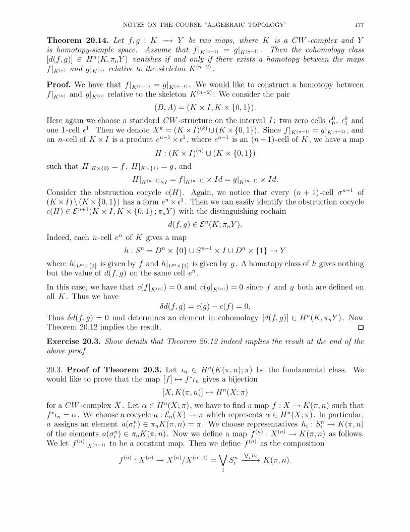
NOTES ON THE COURSE “ALGEBRAIC TOPOLOGY” 177
Theorem 20.14. Let f, g : K −→ Y be two maps, where K is a CW -complex and Yis homotopy-simple space. Assume that f |K(n−1) = g|K(n−1) . Then the cohomology class[d(f, g)] ∈ Hn(K, πnY ) vanishes if and only if there exists a homotopy between the mapsf |K(n) and g|K(n) relative to the skeleton K(n−2) .
Proof. We have that f |K(n−1) = g|K(n−1) . We would like to construct a homotopy betweenf |K(n) and g|K(n) relative to the skeleton K(n−2) . We consider the pair
(B,A) = (K × I,K × 0, 1).Here again we choose a standard CW -structure on the interval I : two zero cells ǫ00 , ǫ01 andone 1-cell ǫ1 . Then we denote Xk = (K× I)(k)∪ (K×0, 1). Since f |K(n−1) = g|K(n−1) , andan n-cell of K× I is a product en−1× ǫ1 , where en−1 is an (n− 1)-cell of K , we have a map
H : (K × I)(n) ∪ (K × 0, 1)such that H|K×0 = f , H|K×1 = g , and
H|K(n−1)×I = f |K(n−1) × Id = g|K(n−1) × Id.Consider the obstruction cocycle c(H). Again, we notice that every (n + 1)-cell σn+1 of(K× I)\ (K×0, 1) has a form en× ǫ1 . Then we can easily identify the obstruction cocyclec(H) ∈ En+1(K × I,K × 0, 1 ; πnY ) with the distinguishing cochain
d(f, g) ∈ En(K; πnY ).
Indeed, each n-cell en of K gives a map
h : Sn = Dn × 0 ∪ Sn−1 × I ∪Dn × 1 → Y
where h|Dn×0 is given by f and h|Dn×1 is given by g . A homotopy class of h gives nothingbut the value of d(f, g) on the same cell en .
In this case, we have that c(f |K(n)) = 0 and c(g|K(n)) = 0 since f and g both are defined onall K . Thus we have
δd(f, g) = c(g)− c(f) = 0.
Thus δd(f, g) = 0 and determines an element in cohomology [d(f, g)] ∈ Hn(K, πnY ). NowTheorem 20.12 implies the result.
Exercise 20.3. Show details that Theorem 20.12 indeed implies the result at the end of theabove proof.
20.3. Proof of Theorem 20.3. Let ιn ∈ Hn(K(π, n); π) be the fundamental class. Wewould like to prove that the map [f ] 7→ f ∗ιn gives a bijection
[X,K(π, n)]↔ Hn(X; π)
for a CW -complex X . Let α ∈ Hn(X; π), we have to find a map f : X → K(π, n) such thatf ∗ιn = α . We choose a cocycle a : En(X)→ π which represents α ∈ Hn(X; π). In particular,a assigns an element a(σni ) ∈ πnK(π, n) = π . We choose representatives hi : Sni → K(π, n)of the elements a(σni ) ∈ πnK(π, n). Now we define a map f (n) : X(n) → K(π, n) as follows.We let f (n)|X(n−1) to be a constant map. Then we define f (n) as the composition
f (n) : X(n) → X(n)/X(n−1) =∨
i
Sni
W
i hi−−−→ K(π, n).
178 BORIS BOTVINNIK
We notice that by construction, a coincides with the distinguishing cochain d(∗, f (n)). Sincea is a cocycle, we have:
0 = δa = δd(∗, f (n)) = c(f (n))− c(∗) = c(f (n)).
Thus c(f (n)) = 0 and there exists an extension of the map f (n) : X(n) → K(π, n) to a mapf (n+1) : X(n+1) → K(π, n). Then we notice that the further obstructions to extend the mapf (n+1) : X(n+1) → K(π, n) to the skeletons X(n+q) live in the corresponding groups
En+q(X; πn+q−1K(π, n)) = 0 for q ≥ 2.
This proves that the map [f ] 7→ f ∗ιn is surjective.
Now we assume that f, g : X → K(π, n) are such that f ∗ιn = g∗ιn in the cohomology groupHn(X; π). By Cellular aproximation Theorem, we may assume that f |X(n−1) = g|X(n−1) =∗ . Then as we have seen, the element f ∗ιn coincides with the cohomology class of thedistiguishing cocycle d(∗, f). Thus f ∗ιn = [d(∗, f)] and g∗ιn = [d(∗, g)]. Then
[d(f, g)] = [d(f, ∗)] + [d(∗, g)] = −f ∗ιn + g∗ιn = 0.
Thus by Theorem 20.14, there exists a homotopy f |X(n) ∼ g|X(n) relative to the skeletonX(n−2) . Clearly all obstructions to extend this homotopy to the skeletons X(n+q) vanish. IfX is a CW -complex of infinite dimension, then we should use the intervals
[2k−12k , 2k+1−1
2k+1
]=[1− 1
2k , 1− 12k+1
]
to construct a homotopy between f |X(n+k) and g|X(n+k) . This proves Theorem 20.3.
Theorem 20.15. (Hopf) Let X be an n-dimensional CW -complex. Then there is a bijection:
Hn(X;Z) ∼= [X,Sn].
Exercise 20.4. Prove Theorem 20.15.
Consider a k -torus T k . We identify T k with the quotient space Rk/ ∼, where two vectors~x ∼ ~y if and only if all coordinates of the vector ~x − ~y are integers. It is easy to see that alinear map f : Rk → Rℓ given by an k× ℓ-matrix A with integral entries descends to a mapf : T k → T ℓ . In that case a map f : T k → T ℓ is called linear.
Exercise 20.5. Prove that any map f : T k → T ℓ is homotopic to a linear map.

NOTES ON THE COURSE “ALGEBRAIC TOPOLOGY” 179
20.4. Stable Cohomology operations and Steenrod algebra. We would like to concludethis sections by brief description of the Steenrod algebra. Let π = π′ = Z/2. Then
O(Z/2, n;Z/2, n′) ∼= [K(Z/2, n), K(Z/2, n′)] ∼= Hn′
(K(Z/2, n);Z/2).
Since the group Hn′
(K(Z/2, n);Z/2) = 0 for n′ < n, all corresponding operations are trivial.
Definition 20.16. A sequence of operations θ = θn , where θn ∈ O(Z/2, n;Z/2, n+ q), iscalled a stable operation if the following diagrams commute for each n:
Hn(X;Z/2)
?
Σ
Hn+q(X;Z/2)
?
Σ
-θn
Hn+1(ΣX;Z/2) Hn+1+q(ΣX;Z/2)-θn+1
Here Σ : H∗(X;Z/2)→ H∗+1(ΣX;Z/2) is the suspension isomorphism.

180 BORIS BOTVINNIK
21. Cohomology of some Lie groups and Stiefel manifolds
21.1. Stiefel manifolds. The Stiefel manifold Vk(Rn) is the manifold of orthonormal k -
frames (v1, . . . , vk) in the Euclidian space Rn . We note that there are canonical projectionmaps pk,j : Vk(R
n) → Vj(Rn) for j ≤ k . To describe its topology and CW -structure, we
identify Vk(Rn) with the coset O(n)/O(n− k) as follows.
We recall that O(n) acts Rn . We would like to be specific: one can identify Rn the space ofcolumn vectors with the standard basis e1, . . . , ek, . . . , en , then O(n) acts on Rn from theleft by matrix multiplication. Then we consider an embedding O(n) ⊂ O(n+1) given by theformula
A 7→[
0 1A 0
]
Then for each orthonormal k -frame (v1, . . . , vk), there is a matrix A ∈ O(n) such that Ae1 =v1, . . . , Aek = vk . Then the transformation A is defined up to an orthogonal transformationB ∈ O(n − k). This identifies Vk(R
n) with the coset O(n)/O(n − k) and gives particulartopology to the Stiefel manifold.
Exercise 21.1. Show that Vk(Rn) is indeed a smooth manifold of dimension 1
2k(2n−k−1).
In particular, we identify V1(Rn) ∼= O(n)/O(n − 1) ∼= Sn−1 . It is convenient to denote by
Pn the projective space RPn−1 . There is a map ϕn : Pn → O(n) which takes a line L ∈ Pnto the reflection through the hyperplane L⊥ . Let x be a unit direction vector for L. Thenϕ(L) ∈ O(n) is given by the formula:
ϕ(L) : y 7→ y − 2 〈y, x〉x ∈ Rn.
Moreover, if m ≤ n, we have a commutative diagram of maps
Pm
?
jm,n
O(m)
?
im,n
-ϕm
Pn
?
pr
O(n)
?
pr
-ϕn
Pn/Pm O(n)/O(m)-ϕ
We denote by Pn,q = Pn/Pn−q the truncated projective space. In particular, we have identifiedPn,1 with the sphere Sn−1 .
Lemma 21.1. The above map ϕ : Pn,1 → O(n)/O(n− 1) is a homeomorphism.
Proof. We identify Pn = RPn−1 with the hemisphere
Sn−1+ =
(x1, . . . , xn) ∈ Sn−1 | xn ≥ 0
,
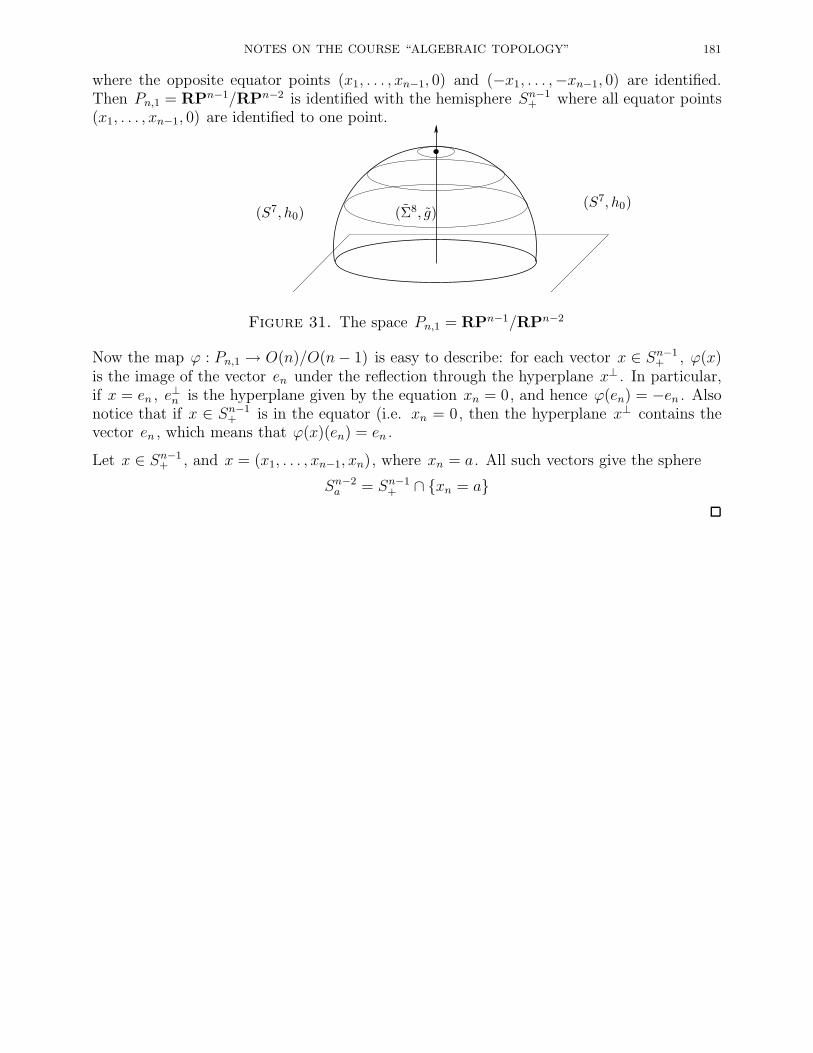
NOTES ON THE COURSE “ALGEBRAIC TOPOLOGY” 181
where the opposite equator points (x1, . . . , xn−1, 0) and (−x1, . . . ,−xn−1, 0) are identified.Then Pn,1 = RPn−1/RPn−2 is identified with the hemisphere Sn−1
+ where all equator points(x1, . . . , xn−1, 0) are identified to one point.
(Σ8, g)(S7, h0)(S7, h0)
Figure 31. The space Pn,1 = RPn−1/RPn−2
Now the map ϕ : Pn,1 → O(n)/O(n− 1) is easy to describe: for each vector x ∈ Sn−1+ , ϕ(x)
is the image of the vector en under the reflection through the hyperplane x⊥ . In particular,if x = en , e⊥n is the hyperplane given by the equation xn = 0, and hence ϕ(en) = −en . Alsonotice that if x ∈ Sn−1
+ is in the equator (i.e. xn = 0, then the hyperplane x⊥ contains thevector en , which means that ϕ(x)(en) = en .
Let x ∈ Sn−1+ , and x = (x1, . . . , xn−1, xn), where xn = a. All such vectors give the sphere
Sn−2a = Sn−1
+ ∩ xn = a