Algebraic Topology

Vanessa RobinsDepartment of Applied Mathematics

Research School of Physics and EngineeringThe Australian National UniversityCanberra ACT 0200, Australia.email: vanessa.robins@anu.edu.au

September 11, 2013

Abstract

This manuscript will be published as Chapter 5 in Wiley’s textbook Mathe-matical Tools for Physicists, 2nd edition, edited by Michael Grinfeld from theUniversity of Strathclyde.

The chapter provides an introduction to the basic concepts of AlgebraicTopology with an emphasis on motivation from applications in the physicalsciences. It finishes with a brief review of computational work in algebraictopology, including persistent homology.

1

arX

iv:1

304.

7846

v2 [

mat

h-ph

] 1

0 Se

p 20

13

Contents

1 Introduction 3

2 Homotopy Theory 42.1 Homotopy of paths . . . . . . . . . . . . . . . . . . . . . . . . . . 42.2 The fundamental group . . . . . . . . . . . . . . . . . . . . . . . 52.3 Homotopy of spaces . . . . . . . . . . . . . . . . . . . . . . . . . 72.4 Examples . . . . . . . . . . . . . . . . . . . . . . . . . . . . . . . 72.5 Covering spaces . . . . . . . . . . . . . . . . . . . . . . . . . . . . 92.6 Extensions and applications . . . . . . . . . . . . . . . . . . . . . 9

3 Homology 113.1 Simplicial complexes . . . . . . . . . . . . . . . . . . . . . . . . . 123.2 Simplicial homology groups . . . . . . . . . . . . . . . . . . . . . 123.3 Basic properties of homology groups . . . . . . . . . . . . . . . . 143.4 Homological algebra . . . . . . . . . . . . . . . . . . . . . . . . . 163.5 Other homology theories . . . . . . . . . . . . . . . . . . . . . . . 18

4 Cohomology 184.1 De Rham cohomology . . . . . . . . . . . . . . . . . . . . . . . . 20

5 Morse theory 215.1 Basic results . . . . . . . . . . . . . . . . . . . . . . . . . . . . . . 215.2 Extensions and applications . . . . . . . . . . . . . . . . . . . . . 235.3 Forman’s discrete Morse theory . . . . . . . . . . . . . . . . . . . 24

6 Computational topology 256.1 The fundamental group of a simplicial complex . . . . . . . . . . 266.2 Smith normal form for homology . . . . . . . . . . . . . . . . . . 276.3 Persistent homology . . . . . . . . . . . . . . . . . . . . . . . . . 286.4 Cell complexes from data . . . . . . . . . . . . . . . . . . . . . . 29

2

1 Introduction

Topology is the study of those aspects of shape and structure that do not de-pend on precise knowledge of an object’s geometry. Accurate measurements arecentral to physics, so physicists like to joke that a topologist is someone whocannot tell the difference between a coffee cup and a doughnut. However, thequalitative nature of topology and its ties to global analysis mean that manyresults are relevant to physical applications. One of the most notable areas ofoverlap comes from the study of dynamical systems. Some of the earliest workin algebraic topology was by Henri Poincare in the 1890s, who pioneered a qual-itative approach to the study of celestial mechanics by using topological resultsto prove the existence of periodic orbits [56]. Topology continued to play animportant role in dynamical systems with significant results pertinent to bothareas from Smale in the 1960s [54]. More recently, in the 1990s computer anal-ysis of chaotic dynamics was one of the drivers for innovation in computationaltopology [36, 39, 46, 30].

As with any established subject, there are several branches to topology:General topology defines the notion of ‘closeness’ (the neighborhood of apoint), limits, continuity of functions and so on in the absence of a metric.These concepts are absolutely fundamental to modern functional analysis; astandard introductory reference is [2]. Algebraic topology derives algebraicobjects (typically groups) from topological spaces to help determine when twospaces are alike. It also allows us to compute quantities such as the numberof pieces the space has, and the number and type of ‘holes’. Differentialtopology builds on the above and on the differential geometry of manifolds tostudy the restrictions on functions that arise as the result of the structure oftheir domain. This chapter is primarily concerned with algebraic topology; itcovers the elementary tools and concepts from this field. It draws on definitionsand material from Chapter ?? on group theory and Chapter ?? on differentialgeometry.

A central question in topology is to decide when two objects are the samein some sense. In general topology, two spaces, A and B, are considered to bethe same if there is a homeomorphism, f , between them: f : A → B is acontinuous function with a continuous inverse. This captures an intrinsic typeof equivalence that allows arbitrary stretching and squeezing of a shape andpermits changes in the way an object sits in a larger space (its embedding),but excludes any cutting or gluing. So for example, a circle (x2 + y2 = 1) ishomeomorphic to the perimeter of a square and to the trefoil knot, but notto a line segment, and a sphere with a single point removed is homeomorphicto the plane. One of the ultimate goals in topology is to find a set of quan-tities (called invariants) that characterize spaces up to homeomorphism. Forarbitrary topological spaces this is known to be impossible [56] but for closed,compact 2-manifolds this problem is solved by finding the Euler characteristic(see p. 15) and orientability of the surface [52, 25].

What is the essential difference between a line segment and a circle? Intu-itively it is the ability to trace your finger round and round the circle as many

3

times as you like without stopping or turning back. Algebraic topology is themathematical machinery that lets us quantify and detect this. The idea behindalgebraic topology is to map topological spaces into groups (or other algebraicstructures) in such a way that continuous functions between topological spacesmap to homomorphisms between their associated groups.1

In Sections 2, 3 and 4, this chapter covers the three basic constructions ofalgebraic topology: homotopy, homology and cohomology theories. Each has adifferent method for defining a group from the structures in a topological space,and although there are close links between the three, they capture different qual-ities of a space. Many of the more advanced topics in algebraic topology involvestudying functions on a space, so we introduce the fundamental link betweencritical points of a function and the topology of its domain in Section 5 on MorseTheory. The computability of invariants, both analytically and numerically, isvital to physical applications so the recent literature on computational topologyis reviewed in Section 6. Finally, we give a brief guide to further reading onapplications of topology to physics.

2 Homotopy Theory

A homotopy equivalence is a weaker form of equivalence between topologicalspaces than a homeomorphism that allows us to collapse a space onto a lower-dimensional subset of itself (as we will explain in Section 2.3), but it capturesmany essential aspects of shape and structure. When applied to paths in a space,homotopy equivalence allows us to define an algebraic operation on loops, andprovides our first bridge between topology and groups.

2.1 Homotopy of paths

We begin by defining a homotopy between two continuous functions f, g : X →Y . These maps will be homotopic if their images f(X), g(X), can be continu-ously morphed from one to the other within Y , i.e. there is a parametrized setof images that starts with one and ends with the other. Formally this defor-mation is achieved by defining a continuous function F : X × [0, 1] → Y withF (x, 0) = f(x) and F (x, 1) = g(x).

For example, consider two maps from the unit circle into the unit sphere,f, g : S1 → S2. We use the angle θ ∈ [0, 2π) to parametrize S1 and theembedding x2 + y2 + z2 = 1 in R3 to define points in S2. Define f(θ) =(cos θ, sin θ, 0) to be a map from the circle to the equator and g(θ) = (0, 0, 1), aconstant map from the circle to the north pole. A homotopy between f and gis given by F (θ, t) = (cos(πt/2) cos θ, cos(πt/2) sin θ, sin(πt/2)) and illustratedin Fig. 1. Any function that is homotopic to a constant function, as in thisexample, is called null-homotopic.

1A homomorphism between two groups, φ : G→ H is a function that respects the groupoperation. That is, φ(a · b) = φ(a) ∗ φ(b), for a, b ∈ G where · is the group operation in G and∗ is the group operation in H.

4

Figure 1: The function f : S1 → S2 that maps the circle onto the equator ofthe sphere is homotopic to the function g : S1 → S2 that maps the circle to thenorth pole. Three sections of the homotopy F : S1 × [0, 1] → S2 are shown ingrey.

When the domain is the unit interval, X = [0, 1], and Y is an arbitrarytopological space the functions f and g are referred to as paths in Y . A spacein which every pair of points may be joined by a path is called path-connected.It is often useful to consider homotopies between paths that fix their endpoints,y0 and y1, say, so we have the additional conditions on F that for all t ∈ [0, 1],F (0, t) = f(0) = g(0) = y0, and F (1, t) = f(1) = g(1) = y1. If a path starts andends at the same point, y0 = y1, it is called a loop. A loop that is homotopicto a single point, i.e. a null-homotopic loop like the one in the example above,is also said to be contractible or trivial. A path-connected space in whichevery loop is contractible is called simply connected. So the real line and thesurface of the sphere are simply connected, but the circle and the surface of adoughnut (the torus) are not.

2.2 The fundamental group

We are now in a position to define our first algebraic object, the fundamentalgroup. The first step is to choose a base point y0 in the space Y and considerall possible loops in Y that start and end at y0. Two loops belong to thesame equivalence class if they are homotopic: given a loop f : [0, 1] → Y withf(0) = f(1) = y0, we write [f ] to represent the set of all loops that are homotopicto f . The appropriate group operation [f ] ∗ [g] on these equivalence classes is aconcatenation of loops defined by tracing each at twice the speed. Specifically,choose f and g to be representatives of their respective equivalence classes anddefine f ∗ g(x) = f(2x) when x ∈ [0, 1

2 ] and f ∗ g(x) = g(2x−1) when x ∈ [ 12 , 1].

Since all loops have the same base point, this product is another loop based aty0. We then simply set [f ] ∗ [g] = [f ∗ g]. The equivalence class of the product

5

a b c

Figure 2: a) Two non-homotopic loops on the torus with the same base point.b) A loop homotopic to the concatenation the loops depicted in (a). c) Anotherloop in the same homotopy class.

[f ∗ g] is independent of the choice of f and g because we can re-parameterizethe homotopies in the same way as we concatenated the loops. Note, though,that the equivalence class [f ∗ g] consists of more than just concatenated loops;Fig. 2 depicts an example on the torus.

The set of all homotopy equivalence classes of loops based at y0 with theoperation ∗ forms a group with the identity element being the class of null-homotopic loops [e] where e(x) = y0, and the inverse of a loop defined to be thesame loop traced backwards: [f ]−1 = [h] where h(x) = f(1− x). This group isthe fundamental group of Y with base point y0: π1(Y, y0).

The operation taking a topological space to its fundamental group is anexample of a functor. This word expresses the property alluded to in theintroduction that continuous maps between topological spaces transform to ho-momorphisms between their associated groups. The functorial nature of thefundamental group is manifest in the following fashion. Suppose we have a con-tinuous function f : X → Y with f(x0) = y0. Then given a loop in X withbase point x0 we can use simple composition of the loop with f to obtain a loopin Y with base point y0. Composition also respects the concatenation of loopsand homotopy equivalences so it induces a homomorphism between the funda-mental groups: π1(f) : π1(X,x0)→ π1(Y, y0). When the function f : X → Y isa homeomorphism, it follows that the induced map π1(f) is an isomorphism oftheir fundamental groups.

Some further elementary properties of the fundamental group are:

• A simply connected space has a trivial fundamental group, i.e. only theidentity element.

• If Y is path-connected, the fundamental group is independent of the basepoint, and we write π1(Y ).

• The fundamental group respects products2 of path-connected spaces: π1(X×Y ) = π1(X)× π1(Y ).

2The (Cartesian or direct) product of two spaces (or two groups) X × Y is defined byordered pairs (x, y) where x ∈ X and y ∈ Y .

6

• The wedge product of two path-connected spaces (obtained by gluing thespaces together at a single point) gives a free product3 on their fundamen-tal groups: π1(X ∨ Y ) = π1(X) ∗ π1(Y ).

• The van Kampen theorem shows how to compute the fundamentalgroup of a space X = U ∪ V when U , V , and U ∩ V are open, path-connected subspaces of X via a free product with amalgamation: π1(X) =π1(U) ∗ π1(V )/N , where N is a normal subgroup generated by elementsof the form iU (γ)iV (γ)−1 and γ is a loop in π1(U ∩ V ), iU and iV areinclusion-induced maps from π1(U ∩ V ) to π1(U) and π1(V ) respectively.See [28] for details.

2.3 Homotopy of spaces

Now we look at what it means for two spaces X and Y to be homotopyequivalent or to have the same homotopy type: there must be continuousfunctions f : X → Y and g : Y → X such that fg : Y → Y is homotopic tothe identity on Y and gf : X → X is homotopic to the identity on X. We canshow that the unit circle S1 and the annulus A have the same homotopy typeas follows. Let

S1 = (r, θ) | r = 1, θ ∈ [0, 2π) and A = (r, θ) | 1 ≤ r ≤ 2, θ ∈ [0, 2π)

be subsets of the plane parametrized by polar coordinates. Define f : S1 → A tobe the inclusion map f(1, θ) = (1, θ) and let g : A→ S1 map all points with thesame angle to the corresponding point on the unit circle: g(r, θ) = (1, θ). Thengf : S1 → S1 is given by gf(1, θ) = (1, θ) which is exactly the identity map. Theother composition is fg : A → A is fg(r, θ) = (1, θ). This is homotopic to theidentity iA = (r, θ) via the homotopy F (r, θ, t) = (1+t(r−1), θ). This example isan illustration of a deformation retraction: a homotopy equivalence betweena space (e.g. the annulus) to a subset (the circle) that leaves the subset fixedthroughout.

Spaces that are homotopy equivalent have isomorphic fundamental groups.A space that has the homotopy type of a point is said to be contractibleand has trivial fundamental group. This is much stronger than being simply-connected: for example, the sphere S2 is simply connected because every loopcan be shrunk to a point, but it is not a contractible space.

2.4 Examples

Real space Rm, m ≥ 1, all spheres Sn with n ≥ 2, any Hilbert space, and anyconnected tree (cf. Chapter ??) have trivial fundamental groups.

The fundamental group of the circle is isomorphic to the integers underaddition: π1(S1) = Z. This can be seen by noting that the homotopy class of

3The free product of two groups G ∗H is an infinite group that contains both G and Has subgroups and whose elements are words of the form g1h1g2h2 · · · .

7

Figure 3: The projective plane, RP 2 is modelled by the unit disk with oppositepoints on the boundary identified. The black loop starting at (0, 0) is homotopicto its inverse with the equivalence suggested by the grey loops.

a loop is determined by how many times it wraps around the circle. A formalproof of this result is quite involved — see Hatcher [28] for details. Any spacethat is homotopy equivalent to the circle will have the same fundamental group,this holds for the annulus, the Mobius band, a cylinder, and the ‘puncturedplane’ R2 \ (0, 0).

The projective plane RP 2 is a non-orientable surface defined by identifyingantipodal points on the boundary of the unit disk (or equivalently, antipodalpoints on the sphere). It has fundamental group isomorphic to Z2 (the groupwith two elements, the identity and r which is its own inverse r2 = id). To seethis, consider a loop that starts at the center of the unit disk (0, 0), goes straightup to (0, 1) which is identified with (0,−1) then continues straight back up tothe origin. This loop is in a distinct homotopy class to the null-homotopic loopbut it is in the same homotopy class as its inverse (to see this, imagine fixingthe loop at (0, 0) and rotate it by 180 as illustrated in Fig. 3).

The fundamental group of a connected graph with v vertices and e edges(cf. Chapter ??) is a free group with n generators4 where n = e − (v − 1) isthe number of edges in excess of a spanning tree. This demonstrates that thefundamental group need not be Abelian (products do not necessarily commute).

The torus T = S1 × S1 so π1(T) = Z × Z. More generally, an orientablegenus-g surface5 (g ≥ 2) has fundamental group isomorphic to a hyperbolictranslation group with 2g generators.

If a space has a finite cell structure, then the fundamental group can be com-puted as a free group with relations in an algorithmic manner; this is discussedin Section 6.

4A free group with one generator, a say, is the infinite cyclic group with elements. . . , a−1, 1, a, a2, . . .. A free group with two generators a, b, contains all elements of the formai1bj1ai2bj2 · · · for integers ik, jl. A free group with n generators is the natural generalizationof this.

5Starting with a sphere, you can obtain all closed oriented 2-manifolds by attaching somenumber of handles (cylinders) to the sphere. The number of handles is the genus.

8

2.5 Covering spaces

The result about the fundamental group of a genus-g surface comes from an-alyzing the relationship between loops on a surface and paths in its universalcovering space (the hyperbolic plane when g ≥ 2). Covering spaces are use-ful in many other contexts (from harmonic analysis to differential topology tocomputer simulation), so we describe them briefly here. They are simply amore general formulation of the standard procedure of identifying a real-valuedperiodic function with a function on the circle.

Given a topological space X, a covering space for X is a pair (C, p), whereC is another topological space and p : C → X is a continuous function ontoX. The covering map p must satisfy the following condition: for every pointx ∈ X, there is a neighborhood U of x such that p−1(U) is a disjoint union ofopen sets each of which is mapped homeomorphically onto U by p. The discreteset of points p−1(x) is called the fiber of x. A universal covering space is onein which C is simply-connected. The reason for the name comes from the factthat a universal covering of X will cover any other connected covering of X. Forexample, the circle is a covering space of itself with C = S1 = z ∈ C : |z| = 1and pk(z) = zk for all non-zero integers k, while the universal cover of thecircle is the real line with pU : R → S1 given by pU (t) = exp(i2πt). The pointz = (1, 0) ∈ S1 is then covered by the fiber t ∈ Z ⊂ R. We illustrate a coveringof the torus in Fig. 4.

When X and C are suitably nice spaces (connected and locally path con-nected), loops in X based at x0 lift to paths in C between elements of the fiberof x0. So in the example of S1, a path in R between two integers i < j mapsunder pU to a loop that wraps j − i times around the circle.

Now consider homeomorphisms of the covering space h : C → C that respectthe covering map, p(h(c)) = p(c). The set of all such homeomorphisms formsa group under composition called the deck transformation group. When(C, p) is a universal covering space for X, it is possible to show that the decktransformation group must be isomorphic to the fundamental group of X. Thisgives a technique for determining the fundamental group of a space in somesituations; see Hatcher [28] for details and examples.

2.6 Extensions and applications

As we saw in the examples of Section 2.4, the fundamental group of an n-dimensional sphere is trivial for n ≥ 2, so the question naturally arises howwe might capture the different topological structures of Sn. To generalize thefundamental group, we examine maps from an n-dimensional unit cube In intothe space X where the entire boundary of the cube is mapped to a fixed basepoint in X, i.e. f : In → X, with f(∂In) = x0. Elements of the higherhomotopy groups πn(X,x0) are then homotopy-equivalence classes of thesemaps. The group operation is concatenation in the first coordinate just as wedefined for one-dimensional closed paths above. The main difference in higherdimensions is that this operation now commutes.

9

Figure 4: The universal covering space of the torus is the Euclidean planeprojected onto the closed surface by identifying opposite edges of each rectanglewith parallel orientations. The fibre of the base point on the torus is a latticeof points in the cover. The two loops on the torus lift to the vertical andhorizontal paths shown in the cover. The lift of the concatenation of thesetwo loops (see Fig. 2 c) is homotopic to the diagonal path in the cover. Thedeck transformation group for this cover is simply the group of translations thatpreserve the rectangles which is isomorphic to Z× Z = π1(T).

It is perhaps not too difficult to see that π2(S2) = Z, although the multiplewrapping of the sphere by a piece of paper cannot be physically realized inR3 in the same way a piece of string wraps many times around a circle. Thesurprise comes with the result that πk(Sn) is non-trivial for most (but certainlynot all) k ≥ n ≥ 2, and in fact mathematicians have not yet determined all thehomotopy groups of spheres for arbitrary k and n [28]. Higher-order homotopygroups are a rich and fascinating set of topological invariants that are the subjectof active research in mathematics.

One application of homotopy theory arises in the study of topological de-fects in condensed matter physics. A classic example is nematic liquid crystalswhich are fluids comprised of molecules with an elongated ellipsoidal shape. Theorder parameter for this system is the (time averaged) direction of the majoraxis of the ellipsoidal molecule: n. For identical and symmetrical molecules, thesign and the magnitude of the vector is irrelevant, and so the parameter spacefor n is the surface of the sphere with antipodal points identified — topologi-cally RP 2. The existence of non-contractible loops in RP 2 is associated withthe existence of topological line defects in configurations of molecules in the ne-matic liquid crystal; see Fig. 5. The fact that π1(RP 2) = Z2 is manifest in thefact that two defects of the same type can smoothly cancel one another. Thesecond homotopy group π2(RP 2) = Z, and this is manifest in the existence ofpoint defects (“hedgehogs”) where the director field points radially away froma central point. See Mermin’s original article [35] or Nakahara [42] for furtherdetails.

10

Figure 5: A cross-section through a nematic fluid with a line defect that runsperpendicular to the page. Each line-segment represents the averaged directionof a single molecule.

3 Homology

The fundamental group is a useful invariant but it captures only the one-dimensional structure of equivalent loops in a space and cannot distinguishbetween spheres of dimensions greater than two, for example. The higher ho-motopy groups do capture this structure but are difficult to compute. Thehomology groups provide a way to describe structure in all relevant dimensions,but require a bit more machinery to define. This can seem abstract at first, butin fact the methods are quite combinatorial and there has been much recentactivity devising efficient algorithms to compute homological quantities fromlarge data sets (see Section 6).

There are a number of different formulations of homology theory that giveessentially the same results for ‘nice’ spaces (such as differentiable manifolds).The two key ingredients are a discrete cell complex that captures the way aspace is put together, and a boundary map that describes incidences betweencells of adjacent dimensions. The algebraic structure comes from defining theaddition and subtraction of cells.

The earliest formulation of homology theory is simplicial homology, basedon triangulations of topological spaces called simplicial complexes. This the-ory has some short-comings when dealing with very general topological spacesand successive improvements over the past century have culminated in the cur-rent form based on singular homology and general cell complexes. Hatcher [28]provides an excellent introduction to homology from this modern perspective.We focus on simplicial homology here since it is the most concrete and easy to

11

adapt for implementation on a computer. The notation used in this section isbased on that of Munkres [40].

3.1 Simplicial complexes

The basic building block is an oriented k-simplex, σk, the convex hull of k+1geometrically independent points, x0, x1, . . . , xk ⊂ Rm, with k ≤ m. Forexample, a 0-simplex is just a point, a 1-simplex is a line segment, a 2-simplexa triangle, and a 3-simplex is a tetrahedron. We write σk = 〈x0, x1, . . . , xk〉to denote a k-simplex and its vertices. The ordering of the vertices defines anorientation of the simplex. This orientation is chosen arbitrarily but is fixed,and coincides with the usual notion of orientation of line segments, trianglesand tetrahedra. Any even permutation of the vertices in a simplex gives anothersimplex with the same orientation, while an odd permutation gives a simplexwith negative orientation.

Given a set V , an abstract simplicial complex, C, is a collection of finitesubsets of V with the property if σk = v0, . . . , vk ∈ C then all subsets of σk

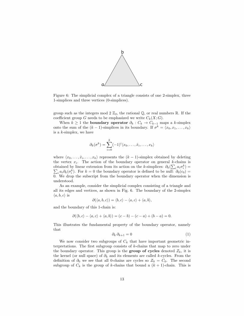
(its faces) are also in C. If the simplicial complex is finite then it can always beembedded in Rm for some m (certain complexes with infinitely many simplicescan also be embedded in finite-dimensional space). An embedded complex iscalled a geometric realization of C. The subset of Rm occupied by the geometriccomplex is denoted by |C| and is called a polytope or polyhedron. When atopological space X is homeomorphic to a polytope, |C|, it is called a trian-gulated space and the simplicial complex C is a triangulation of X. Forexample, a circle is homeomorphic to the boundary of a triangle so the threevertices a, b, c and three 1-simplices, 〈ab〉, 〈bc〉, 〈ca〉 are a triangulation of the cir-cle (see Fig. 6). All differentiable manifolds have triangulations, but a completecharacterization of the class of topological spaces that have a triangulation isnot known. Every topological 2 or 3-manifold has a triangulation, but thereis a (non-smooth) 4-manifold that cannot have a triangulation (it is related tothe Lie group E8 [51]). The situation for non-differentiable manifolds in higherdimensions remains uncertain.

3.2 Simplicial homology groups

We now define the group structures associated with a space X that is triangu-lated by a finite simplicial complex C. Although the triangulation of a space isnot unique, the homology groups for any triangulation of the same space areidentical (see [40]); this makes simplicial homology well-defined.

The set of all k-simplices from C form the basis of a free group called the k-thchain group, Ck(X). The group operation is an additive one; recall that −σkis just σk with the opposite orientation, so this defines the inverse elements. Ingeneral, a k-chain is the formal sum of a finite number of oriented k-simplices:ck =

∑i aiσ

ki . The coefficients, ai, are elements of another group, called the

coefficient group that is typically the integers, Z, but can be any Abelian

12

a

b

c

Figure 6: The simplicial complex of a triangle consists of one 2-simplex, three1-simplices and three vertices (0-simplices).

group such as the integers mod 2 Z2, the rational Q, or real numbers R. If thecoefficient group G needs to be emphasized we write Ck(X;G).

When k ≥ 1 the boundary operator ∂k : Ck → Ck−1 maps a k-simplexonto the sum of the (k − 1)-simplices in its boundary. If σk = 〈x0, x1, . . . , xk〉is a k-simplex, we have

∂k(σk) =

k∑i=0

(−1)i〈x0, . . . , xi, . . . , xk〉

where 〈x0, . . . , xi, . . . , xk〉 represents the (k − 1)-simplex obtained by deletingthe vertex xi. The action of the boundary operator on general k-chains isobtained by linear extension from its action on the k-simplices: ∂k(

∑i aiσ

ki ) =∑

i ai∂k(σki ). For k = 0 the boundary operator is defined to be null: ∂0(c0) =0. We drop the subscript from the boundary operator when the dimension isunderstood.

As an example, consider the simplicial complex consisting of a triangle andall its edges and vertices, as shown in Fig. 6. The boundary of the 2-simplex〈a, b, c〉 is

∂(〈a, b, c〉) = 〈b, c〉 − 〈a, c〉+ 〈a, b〉,

and the boundary of this 1-chain is:

∂(〈b, c〉 − 〈a, c〉+ 〈a, b〉) = (c− b)− (c− a) + (b− a) = 0.

This illustrates the fundamental property of the boundary operator, namelythat

∂k ∂k+1 = 0 (1)

We now consider two subgroups of Ck that have important geometric in-terpretations. The first subgroup consists of k-chains that map to zero underthe boundary operator. This group is the group of cycles denoted Zk, it isthe kernel (or null space) of ∂k and its elements are called k-cycles. From thedefinition of ∂0 we see that all 0-chains are cycles so Z0 = C0. The secondsubgroup of Ck is the group of k-chains that bound a (k + 1)-chain. This is

13

the group of boundaries Bk, it is the image of ∂k+1. It follows from (1) thatevery boundary is a cycle, i.e. the image of ∂k+1 is mapped to zero by ∂k so Bkis a subgroup of Zk. In our example of the triangle simplicial complex, we findno 2-cycles and a 1-cycle, 〈b, c〉 − 〈a, c〉+ 〈a, b〉, such that all other 1-cycles areinteger multiples of this. This 1-cycle is also the only 1-boundary so Z1 = B1,and the 0-boundaries B0 are generated by the two 0-chains: c− b and c−a (thethird boundary a− b = (c− b)− (c− a)).

Since Bk ⊂ Zk, we can form a quotient group, Hk = Zk/Bk; this is the pre-cisely the k-th homology group. The elements of Hk are equivalence classesof k-cycles that do not bound any k + 1 chain so this is how homology charac-terizes k-dimensional holes. Formally, two k-cycles w, z ∈ Zk are in the sameequivalence class if w−z ∈ Bk; such cycles are said to be homologous. We write[z] ∈ Hk for the equivalence class of cycles homologous to z. For the simpleexample of the triangle simplicial complex, we have already seen that Z1 = B1

so that H1 = 0. The 0-cycles are generated by a, b, c and the boundariesby (c− b), (c− a), so H0 has a single equivalence class, [c], and is isomorphicto Z.

The homology groups for some familiar spaces are:

• Real space Rn has H0 = Z and Hk = 0 for k ≥ 1.

• The spheres have H0(Sn) = Z, Hn(Sn) = Z and Hk(Sn) = 0 for allother values of k.

• The torus has H0 = Z, H1 = Z ⊕ Z, H2 = Z, Hk = 0 for all other k.The 2-cycle that generates H2 is the entire surface. This is in contrast tothe second homotopy group for the torus, which is trivial.

• The real projective plane, RP 2 has H0 = Z, H1 = Z2, and Hk = 0 fork ≥ 2. The fact that H2 is trivial is a result of the surface being non-orientable; even though RP 2 is closed as a manifold, the 2-chain coveringthe surface is not a 2-cycle.

The combinatorial nature of simplicial homology makes it readily computable.We give the classical algorithm and review recent work on fast and efficientalgorithms for data in Section 6.

3.3 Basic properties of homology groups

In general, the homology groups of a finite simplicial complex are finitely gen-erated Abelian groups, so the following theorem tells us about their generalstructure (see Theorem 4.3 of [40]).

Theorem 1 If G is a finitely generated Abelian group then it is isomorphic tothe following direct sum:

G ' (Z⊕ · · · ⊕ Z)⊕ Zt1 ⊕ · · · ⊕ Ztm .

14

The number of copies of the integer group Z is called the Betti number β.The cyclic groups Zti are called the torsion subgroups and the ti are the torsioncoefficients; they are defined so that ti > 1 and t1 divides t2 which divides t3and so on. The torsion coefficients of the homology group Hk(C) measure thetwistedness of the space in some sense. For example, the real projective planehas H1 = Z2, because the 2-chain that represents the whole of the surface hasa boundary that is twice the generating 1-cycle. The Betti number βk of thek-th homology group counts the number non-equivalent non-bounding k-cyclesand this can be loosely interpreted as the number of k-dimensional holes. The0-th Betti number, β0, counts the number of path-connected components of thespace.

Some other fundamental properties of the homology groups are as follows:

• If the simplicial complex has N connected components, X = X1∪· · ·∪XN

thenH0 is isomorphic to the direct sum ofN copies of the coefficient group,and Hk(X) = Hk(X1)⊕ · · · ⊕Hk(XN ).

• Homology is a functor. If f : X → Y is a continuous function fromone simplicial complex into another, it induces natural maps on the chaingroups f] : Ck(X)→ Ck(Y ) for each k which commute with the boundaryoperator: ∂f] = f]∂. This commutativity implies that cycles map to cyclesand boundaries to boundaries, so that the f] induce homomorphisms onthe homology groups f∗ : Hk(X)→ Hk(Y ).

• If two spaces are homotopy equivalent they have isomorphic homologygroups (this is shown using the above functorial property).

• The first homology group is the Abelianization of the fundamental group.When X is a path-connected space, the connection between H1(X) andπ1(X) is made by noticing that two 1-cycles are equivalent in homology iftheir difference is the boundary of a 2-chain; if we parametrize the 1-cyclesas loops then this 2-chain forms a region through which one can define ahomotopy. See [28] for a formal proof.

• The higher-dimensional homology groups have the comforting propertythat if all simplices in a complex have dimensions ≤ m then Hk = 0for k > m. This is in stark contrast to the higher-dimensional homotopygroups.

A particularly pleasing result in homology relates the Betti numbers to an-other topological invariant called the Euler characteristic. For a finite sim-plicial complex, C, define nk to be the number of simplices of dimension k,then the Euler characteristic is defined to be χ(C) = n0 − n1 + n2 − · · · . TheEuler-Poincare theorem states that the the alternating sum of Betti numbersis the same as the Euler characteristic [40]: χ = β0 − β1 + β2 − · · · . This isone of many results that connect the Euler characteristic with other propertiesof manifolds. For example, if M is a compact 2-manifold with a Riemannianmetric, then the Gauss-Bonnet theorem states that 2πχ is equal to the integral

15

of Gaussian curvature over the surface plus the integral of geodesic curvatureover the boundary of M [29]. Further, if M is orientable and has no boundarythen it must be homeomorphic to a sphere with g handles and χ = 2−2g whereg is the genus of the surface. When M is non-orientable without boundary, thenit is homeomorphic to a sphere with r cross-caps and χ = 2− r.

The Euler characteristic is a topological invariant with the property ofinclusion-exclusion: If a triangulated space X = A ∪ B where A and B areboth subcomplexes, then

χ(X) = χ(A) + χ(B)− χ(A ∩B).

This means the value of χ is a localizable one and can be computed by cutting upa larger space into smaller chunks. This property makes it a popular topologicalinvariant to use in applications [34]. A recent application that exploits the localadditivity of the Euler characteristic to great effect is target enumeration inlocalized sensor networks [5, 16]. The Euler characteristic has also been shownto be an important parameter in the physics of porous materials [3, 49].

The simple inclusion-exclusion property above does not hold for the Bettinumbers since they capture global aspects of the topology of a space. Relatingthe homology of two spaces to their union requires more sophisticated algebraicmachinery that we review below.

3.4 Homological algebra

Many results and tools in homology are independent of the details about theway the chains and boundary operators are defined for a topological space; theydepend only on the chain groups and the fact that ∂∂ = 0. The study of suchabstract chain complexes and transformations between them is called homo-logical algebra and is one of the original examples in category theory [40].

An abstract chain complex is a sequence of Abelian groups and homomor-phisms

· · · dk+2−→ Ck+1dk+1−→ Ck

dk−→ · · · d1−→ C0 −→ 0, with dkdk+1 = 0.

The homology of this chain complex is Hk(C) = ker dk/im dk+1. In certaincases (such as the simplicial chain complex of a contractible space) we find thatim dk+1 = ker dk for k ≥ 1 so the homology groups are trivial. Such a sequenceis said to be exact.

This property of exactness has many nice consequences. For example, witha short exact sequence of groups

0→ Af−→ B

g−→ C → 0.

the exactness means that f is a monomorphism (one-to-one) and g is an epimor-phism (onto). In fact g induces an isomorphism of groups C ≈ B/f(A), andif these groups are finitely generated Abelian then the Betti numbers satisfyβ(B) = β(C) +β(A) (where we have replaced f(A) by A since f is one-to-one).

16

Now imagine there is a short exact sequence of chain complexes, i.e.

0→ Akfk−→ Bk

gk−→ Ck → 0.

is exact for all k and the maps fk, gk commute with the boundary operatorsin each complex (i.e. dBfk = fk−1dA, etc.). Typically, the fk will be inducedby an inclusion map (and so be monomorphisms), and gk by a quotient map(making them epimorphisms) on some underlying topological spaces. The zig-zag lemma shows that these short exact sequences can be joined together intoa long exact sequence on the homology groups of A,B and C:

· · · → Hk(A)f∗−→ Hk(B)

g∗−→ Hk(C)∆−→ Hk−1(A)

f∗−→ Hk−1(B)→ · · ·

The maps f∗ and g∗ are those induced by the chain maps f and g and the bound-ary maps ∆ are defined directly on the homology classes in Hk(C) and Hk−1(A)by showing that cycles in Ck map to cycles in Ak−1 via gk, the boundary ∂B ,and fk−1. Details are given in Hatcher [28].

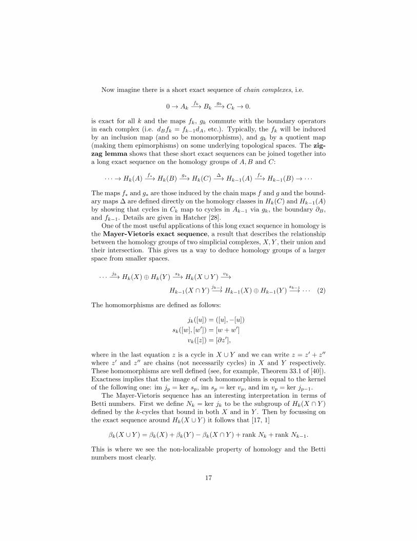
One of the most useful applications of this long exact sequence in homology isthe Mayer-Vietoris exact sequence, a result that describes the relationshipbetween the homology groups of two simplicial complexes, X,Y , their union andtheir intersection. This gives us a way to deduce homology groups of a largerspace from smaller spaces.

· · · jk−→ Hk(X)⊕Hk(Y )sk−→ Hk(X ∪ Y )

vk−→

Hk−1(X ∩ Y )jk−1−→ Hk−1(X)⊕Hk−1(Y )

sk−1−→ · · · (2)

The homomorphisms are defined as follows:

jk([u]) = ([u],−[u])

sk([w], [w′]) = [w + w′]

vk([z]) = [∂z′],

where in the last equation z is a cycle in X ∪ Y and we can write z = z′ + z′′

where z′ and z′′ are chains (not necessarily cycles) in X and Y respectively.These homomorphisms are well defined (see, for example, Theorem 33.1 of [40]).Exactness implies that the image of each homomorphism is equal to the kernelof the following one: im jp = ker sp, im sp = ker vp, and im vp = ker jp−1.

The Mayer-Vietoris sequence has an interesting interpretation in terms ofBetti numbers. First we define Nk = ker jk to be the subgroup of Hk(X ∩ Y )defined by the k-cycles that bound in both X and in Y . Then by focussing onthe exact sequence around Hk(X ∪ Y ) it follows that [17, 1]

βk(X ∪ Y ) = βk(X) + βk(Y )− βk(X ∩ Y ) + rank Nk + rank Nk−1.

This is where we see the non-localizable property of homology and the Bettinumbers most clearly.

17

The Mayer-Vietoris sequence holds in a more general setting than simplicialhomology. It is an example of a result that can be derived from the Eilenberg-Steenrod axioms. Any theory for which these five axioms hold is a type ofhomology theory, see [28] for further details.

3.5 Other homology theories

Chain complexes that capture topological information may be defined in a num-ber of ways. We have defined simplicial chain complexes above, and will brieflydescribe some other techniques here.

Cubical homology is directly analogous to simplicial homology using k-dimensional cubes as building elements rather than k-dimensional simplices.This theory is developed in full in [30] and arose from applications in digitalimage analysis and numerical analysis of dynamical systems.

Singular homology is built from singular k-simplices which are simplycontinuous functions from the standard k-simplex into a topological space X,σ : 〈v0, . . . , vk〉 → X. Singular chains and the boundary operator are definedas they are in simplicial homology. A greater degree of flexibility is found insingular homology since the maps σ are allowed to collapse the simplices, e.g.the standard k-simplex, k > 0 may have boundary points mapping to the samepoint in X, or the entire simplex may be mapped to a single point [28].

An even more general formulation of cellular homology is made by con-sidering general cell (CW) complexes. A cell complex is built incrementally bystarting with a collection of points X(0) ⊂ X, then attaching 1-cells via maps ofthe unit interval into X so that end points map into X(0) to form the 1-skeletonX(1). This process continues by attaching k-cells to the (k − 1)-skeleton bycontinuous maps of the closed unit k-ball, φ : Bk → X that are homeomorphicon the interior and satisfy φ : ∂Bk → X(k−1). The definition of the boundaryoperator for a cell complex requires the concept of degree of a map of the k-sphere (i.e. the boundary of a (k+ 1)-dimensional ball). For details see Hatcher[28].

We will see in the section on Morse Theory that it is also possible to definea chain complex from the critical points of a smooth function on a manifold.

4 Cohomology

The cohomology groups are derived by a simple dualization procedure on thechain groups (similar to the construction of dual function spaces in analysis).We will again give definitions in the simplicial setting but the concepts carryover to other contexts. A cochain φk is a function from the simplicial chaingroup into the coefficient group, φk : Ck(X;G)→ G (recall that G is usually theintegers, Z, but can be any Abelian group). The space of all k-cochains formsa group called the k-th cochain group Ck(X;G). The simplicial boundaryoperators ∂k : Ck → Ck−1 induce coboundary operators δk−1 : Ck−1 → Ck onthe cochain groups via δ(φ) = φ∂. In other words, the cochain δ(φ) is defined

18

via the action of φ on the boundary of each k-simplex σ = 〈x0, x1, . . . , xk〉:

δ(φ)(σ) =∑i

(−1)iφ(〈x0, . . . , xi, . . . , xk〉).

The key property from homology that ∂k∂k+1 = 0 also holds true for thecoboundary: δkδk−1 = 0 (coboundaries are mapped to zero) so we define thek-th cohomology group as Hk(X) = ker δk/im δk−1. Note that cochainsφ ∈ ker δ are functions that vanish on the k-boundaries (not the larger group ofk-cycles), and a coboundary ηk ∈ im δ is one that can be defined via the actionof some cochain φk−1 on the (k − 1)-boundaries.

The coboundary operator acts in the direction of increasing dimension andthis can be a more natural action in some situations (such as de Rham cohomol-ogy of differential forms discussed below) and also has some interesting algebraicconsequences (it leads to the definition of the cup product).

· · ·←−Ck+1 δk←− Ck ←− · · · ←− C0 ←− 0.

This action of the coboundary makes cohomology contravariant (induced mapsact in the opposite direction) where homology is covariant (induced maps actin the same direction). If f : X → Y is a continuous function between twotopological spaces then the group homomorphism induced on the cohomologygroups acts as f∗ : Hk(Y )→ Hk(X).

In simplicial homology, the simplices form bases for the chain groups, andwe can similarly use them as bases for the cochain groups by defining an el-ementary cochain σ as the function that takes the value one on σ and zeroon all other simplices. For a finite simplicial complex it is possible to representthe boundary operator ∂ as a matrix with respect to the bases of oriented k-and (k − 1)-simplices. If we then use the elementary cochains as bases for thecochain groups, the matrix representation for the coboundary operator is justthe transpose of that for the boundary operator. This shows that for finitesimplicial complexes, the functional and geometric meanings of duality are thesame.

Another type of duality is that between homology and cohomology groups oncompact closed oriented manifolds (i.e. without boundary). Poincare dualitystates that Hk(M) = Hm−k(M) for k ∈ 0, . . . ,m where m is the dimensionof the manifold, M ; see [28] for further details.

Despite this close relationship between homology and cohomology on man-ifolds, the cohomology groups have a naturally defined product combining twocochains and this additional structure can help distinguish between some spacesthat homology does not. We start with φ ∈ Ck(X;G) and ψ ∈ Cl(X;G) wherethe coefficient group should now be a ring R (i.e. R should have both additionand multiplication operations; Z, Zp, and Q are rings.) The cup product isthe cochain φ ` ψ ∈ Ck+l(X;R) defined by its action on a (k + l)-simplexσ = 〈v0, . . . , vk+l〉 as follows:

(φ ` ψ)(σ) = φ(〈v0, . . . , vk〉)ψ(〈vk, . . . , vk+l〉).

19

The relation between this product and the coboundary is:

δ(φ ` ψ) = δφ ` ψ + (−1)kφ ` δψ.

From this, we see that the product of two cocycles is another cocycle, and if theproduct is between a cocycle and a coboundary, then the result is a coboundary.Thus, the cup product is a well defined product on the cohomology groups that isanticommutative: [φ] ` [ψ] = (−1)kl[ψ] ` [φ] (provided the coefficient ring, G,is commutative). These rules for products of cocycles should look suspiciouslyfamiliar to those who have read Chapter ??. They are similar to those forexterior products of differential forms and this relationship is formalized in thenext section when we define de Rham cohomology.

4.1 De Rham cohomology

One interpretation of cohomology that is of particular interest in physics comesfrom the study of differential forms on smooth manifolds; cf. Chapter ??. Re-call that a differential form of degree k, ω, defines for each point p ∈ M , analternating multilinear map on k copies of the tangent space to M at p:

ωp : TpM × · · · × TpM → R

The set of all differential k-forms on a manifold M is a vector space, Ωk(M), andthe exterior derivative is a linear operator that takes a k-form to a k+1-form,dk : Ωk(M)→ Ωk+1(M) as defined in Chapter ??.

The crucial property dd = 0 holds for the exterior derivative. In this context,k-forms in the image of d are called exact, i.e. ω = dσ for some (k − 1)-form σ; and those for which dω = 0 are called closed. We therefore have acochain complex of differential forms and can form quotient groups of closedforms modulo the exact forms to obtain the de Rham cohomology groups:

HkdR(M,R) = ker dk/im dk−1

The cup product in de Rham cohomology is exactly the exterior (or wedge)product on differential forms.

De Rham’s theorem states that the above groups are isomorphic to those de-rived via simplicial or singular cohomology [9]. And so we see that the topologyof a manifold has a direct influence on the properties of differential forms thathave it as their domain. For example, the Poincare Lemma states that if M is acontractible open subset of Rn then all smooth closed k-forms on M are exact(the cohomology groups are trivial). In the language of multivariable calculusthis becomes Helmholtz’ theorem that a vector field, V, with curlV = 0 in asimply connected open subset of R3 can be expressed as the gradient of a poten-tial function: V = gradf in the appropriate domain [43]. These considerationsplay a key role in the study of electrodynamics via Maxwell’s equations [27].

20

5 Morse theory

We now turn to a primary topic in differential topology: to examine the relation-ship between the topology of a manifold M and real-valued functions defined onM . The basic approach of Morse theory is to use the level cuts of a functionf : M → R and study how these subsets Ma = f−1(−∞, a] change as a is varied.For ‘nice’ functions the level cuts change their topology in a well-defined wayonly at the critical points. This leads to a number of powerful theorems thatrelate the homology of a manifold to the critical points of a function defined onit.

5.1 Basic results

A Morse function f : M → R is a smooth real-valued function defined on adifferentiable manifold M such that each critical point of f is isolated and thematrix of second derivatives (the Hessian) is non-degenerate at each criticalpoint. An example is illustrated in Fig. 7. The details on how to define thesederivatives with respect to a coordinate chart on M are given in Chapter ??.This may seem like a restrictive class of functions but in fact Morse functionsare dense in the space of all smooth functions, so any smooth function can besmoothly perturbed to obtain a Morse function [31]. Now suppose x ∈ M is acritical point of f , i.e. df(x) = 0. The index of this critical point is the numberof negative eigenvalues of the Hessian matrix. Intuitively this is the number ofdirections in which f is decreasing: a minimum has index 0, and a maximumhas index m where m is the dimension of the manifold M . Critical points ofintermediate index are called saddles since they have some increasing and somedecreasing directions.

The two main results about level cuts Ma of a Morse function f are that:

• When [a, b] is an interval for which there are no critical values of f(i.e. there is no x ∈ f−1([a, b]) for which df(x) = 0) then Ma and Mb

are homotopy equivalent.

• Let x be a non-degenerate critical point of f with index i, let f(x) = cand let ε > 0 be such that f−1[c − ε, c + ε] is compact and contains noother critical points. Then Mc+ε is homotopy equivalent to Mc−ε with ani-cell attached.

(Recall that an i-cell is an i-dimensional unit ball and the attaching map gluesthe whole boundary of the i-cell continuously into the prior space). The proofsof these theorems rely on homotopies defined via the negative gradient flow off [31].

Gradient flow lines are another key ingredient of Morse theory and allowus to define a chain complex and to compute the homology of M . Each pointx ∈M has a unique flow line or integral path γx : R→M such that

γx(0) = x and∂γx(t)

∂ t= −∇f(γx(t)).

21

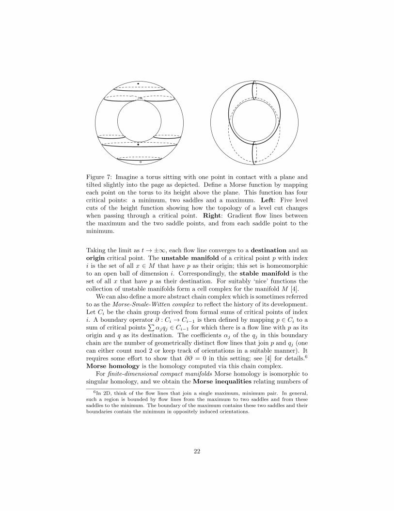
Figure 7: Imagine a torus sitting with one point in contact with a plane andtilted slightly into the page as depicted. Define a Morse function by mappingeach point on the torus to its height above the plane. This function has fourcritical points: a minimum, two saddles and a maximum. Left: Five levelcuts of the height function showing how the topology of a level cut changeswhen passing through a critical point. Right: Gradient flow lines betweenthe maximum and the two saddle points, and from each saddle point to theminimum.

Taking the limit as t→ ±∞, each flow line converges to a destination and anorigin critical point. The unstable manifold of a critical point p with indexi is the set of all x ∈ M that have p as their origin; this set is homeomorphicto an open ball of dimension i. Correspondingly, the stable manifold is theset of all x that have p as their destination. For suitably ‘nice’ functions thecollection of unstable manifolds form a cell complex for the manifold M [4].

We can also define a more abstract chain complex which is sometimes referredto as the Morse-Smale-Witten complex to reflect the history of its development.Let Ci be the chain group derived from formal sums of critical points of indexi. A boundary operator ∂ : Ci → Ci−1 is then defined by mapping p ∈ Ci to asum of critical points

∑αjqj ∈ Ci−1 for which there is a flow line with p as its

origin and q as its destination. The coefficients αj of the qj in this boundarychain are the number of geometrically distinct flow lines that join p and qj (onecan either count mod 2 or keep track of orientations in a suitable manner). Itrequires some effort to show that ∂∂ = 0 in this setting; see [4] for details.6

Morse homology is the homology computed via this chain complex.For finite-dimensional compact manifolds Morse homology is isomorphic to

singular homology, and we obtain the Morse inequalities relating numbers of

6In 2D, think of the flow lines that join a single maximum, minimum pair. In general,such a region is bounded by flow lines from the maximum to two saddles and from thesesaddles to the minimum. The boundary of the maximum contains these two saddles and theirboundaries contain the minimum in oppositely induced orientations.

22

critical points of f : M → R to the Betti numbers of M :

c0 ≥ β0

c1 − c0 ≥ β1 − β0

c2 − c1 + c0 ≥ β2 − β1 + β0

...∑0≤i≤m

(−1)m−ici =∑

0≤i≤m

(−1)m−iβi = χ(M).

where ci is the number of critical points of f of index i and βi is the i-th Bettinumber of M . Notice that the final relationship is an equality ; the alternatingsum of numbers of critical points is the same as the Euler characteristic χ(M).It also follows from the above that ci ≥ βi for each i.

5.2 Extensions and applications

Morse theory is primarily used as a powerful tool to prove results in other set-tings. For example, Morse obtained his results in order to prove the existence ofclosed geodesics on a Riemannian manifold [38]; most famously, Morse theoryforms the foundation of a proof due to Smale of the higher-dimensional Poincareconjecture [53]. Morse theory has been extended in many ways that relax con-ditions on the manifold or the function being studied [8]. We mention a few ofthe main generalisations here.

A Morse-Bott function is one for which the critical points may now notbe isolated and instead form a critical set that is a closed submanifold. At thevery simplest level for example, this lets us study the height function of a torussitting flat on a table since the circle of points touching the table is critical [7].

The Conley index from dynamical systems is a generalization of Morsetheory to flows in a more general class than those generated by the gradientof a Morse function. For general flows, invariant sets are no longer single fixedpoints but may be periodic cycles or even fractal “strange attractors”. In theMorse setting, the index is simply the dimension of the unstable manifold ofthe fixed point, but for general flows a more subtle construction is required.Conley’s insight was that an isolated invariant set can be characterized by theflow near the boundary of a neighborhood of the set. The Conley index is then(roughly speaking) the homotopy type of such a neighborhood relative to itsboundary. For details see [15, 14, 37].

Building on Conley’s work and the Morse complex of critical points and con-necting orbits, Floer created an infinite-dimensional version of Morse homologynow called Floer homology [4]. This has various formulations which have beenused to study problems in symplectic geometry (the geometry of Hamiltoniandynamical systems) and also the topology of 3- and 4-dimensional manifolds[33].

There are a number of approaches adapting Morse theory to a discrete set-ting, of increasing importance in geometric modelling, image and data analysis,

23

and quantum field theory. The approach due to Forman is summarized in thefollowing section.

5.3 Forman’s discrete Morse theory

Discrete Morse theory is a combinatorial analogue of Morse Theory for functionsdefined on cell complexes. Discrete Morse functions are not intended to beapproximations to smooth Morse functions, but the theory developed in [23, 24]keeps much of the style and flavor of the standard results from smooth Morsetheory.

In keeping with earlier parts of this chapter, we will give definitions for asimplicial complex C, but the theory holds for general CW-complexes with littlemodification. First recall that a simplex α is a face of another simplex β ifα ⊂ β, in which case β is called a coface of α. A function f : C → R thatassigns a real number to each simplex in C is a discrete Morse function if forevery α(p) ∈ C, f takes a value less than or equal to f(α) on at most one cofaceof α and takes a value greater than or equal to f(α) on at most one face of α.In other words,

#β(p+1) > α | f(β) ≤ f(α) ≤ 1,

and#γ(p−1) < α | f(γ) ≥ f(α) ≤ 1,

where # denotes the number of elements in the set. A simplex α(p) is criticalif all cofaces take strictly greater values and all faces are strictly lower.

A cell α can fail to be critical in two possible ways. There can exist γ < αsuch that f(γ) ≥ f(α), or there can exist β > α such that f(β) ≤ f(α). Lemma2.5 of [23] shows that these two possibilities are exclusive: they cannot be truesimultaneously for a given cell α. Thus each non-critical cell α may be pairedeither with a non-critical cell that is a coface of α, or with a non-critical cellthat is a face of α.

As noted by Forman (Section 3 of [24]), it is usually simpler to work withpairings of cells with faces than to construct a discrete Morse function on agiven complex. So we define a discrete vector field V as a collection of pairs(α(p), β(p+1)) of cells α < β ∈ C such that each cell of C is in at most onepair of V . A discrete Morse function defines a discrete vector field by pairingα(p) < β(p+1) whenever f(β) ≤ f(α). The critical cells are precisely those thatdo not appear in any pair. Discrete vector fields that arise from Morse functionsare called gradient vector fields. See Fig. 8 for an example.

It is natural to consider the flow associated with a vector field and in thediscrete setting the analogy of a flow-line is a V -path. A V -path is a sequenceof cells:

α(p)0 , β

(p+1)0 , α

(p)1 , β

(p+1)1 , α

(p)2 , . . . , β

(p+1)r−1 , α(p)

r .

where (αi, βi) ∈ V , βi > αi+1, and αi 6= αi+1 for all i = 0, . . . , r − 1. A V -pathis a non-trivial closed V -path if αr = α0 for r > 1. Forman shows that a discretevector field is the gradient vector field of a discrete Morse function if and onlyif there are no non-trivial closed V -paths (Theorem 9.3 of [23]).

24

a b

cd

e f g

h

i

h

i

e

e ef g

Figure 8: A simplicial complex with the topology of the torus (opposite edgesof the rectangle are identified according to the vertex labels). The arrows showhow to pair simplices in a gradient vector field. A compatible discrete Morsefunction has a critical 0-cell (a minimum) at a, two critical 1-cells (saddles) atedges 〈b, h〉 and 〈d, f〉 and a critical 2-cell (a maximum) at 〈e, i, g〉.

The four results about Morse functions that we gave earlier all carry overinto the discrete setting: the homotopy equivalence of level sets away from acritical point, adding a critical i-cell is homotopy equivalent to attaching an i-cell, the existence of and homology of the Morse chain complex, and the Morseinequalities. One of the notable differences between the discrete and continuoustheories is that flow lines for a smooth Morse function on a manifold are uniquelydetermined at each point, whereas V -paths can merge and split.

6 Computational topology

An algorithmic and combinatorial approach to topology has led to significantresults in low-dimensional topology over the past twenty years. There are twomain apsects to computational topology: first, research into methods for makingtopological concepts algorithmic, culminating for example, in the beginnings ofan algorithmic classification of (Haken) 3-manifolds [32] (a result analogousto the classification of closed compact 2-manifolds by Euler characteristic andorientability). And second, the challenge to find efficient and useful techniquesfor extracting topological invariants from data; see [21] for example. We startthis section by describing simple algorithms that demonstrate the computabilityof the fundamental group and homology groups of a simplicial complex, andthen survey some recent advances in building cell complexes and computinghomology from data.

25

a b

cd

e f g

h

i

h

i

e

e ef g

Figure 9: A simplicial complex with the topology of a torus (opposite edges ofthe rectangle are identified according to the vertex labels). A spanning tree Twith root vertex a is shown in bold. Any closed path that starts and ends at acan be decomposed into a sum of loops that lie in T except for a single edge.

6.1 The fundamental group of a simplicial complex

In Section 2 we saw that the fundamental group of a topological space couldbe determined from unions and products of smaller spaces or by using a cov-ering space. When the space has a triangulation (i.e. it is homeomorphic to apolyhedron) there is a more systematic and algorithmic approach to finding thefundamental group as the quotient of a free group by a set of relations that wesummarize below. See [55] for a complete treatment of this edge-path group.

Let C be a connected finite simplicial complex. Any path in |C| is homotopicto one that follows only edges in C, and any homotopy between edge-pathscan be restricted to the 2-simplices of C. This means the fundamental groupdepends only on the topology of the 2-skeleton of C. The algorithm for findinga presentation of π1(C) proceeds as follows.

First find a spanning tree T ⊂ C(1) i.e. a connected, contractible subgraphof the 1-skeleton that contains every vertex of C; see Fig. 9 for an example. Onealgorithm for doing this simply grows from an initial vertex v (the root) byadding adjacent (edge, vertex) pairs only if the other vertex is not already inT . A non-trivial closed edge-path in C (a loop) must include edges that are notin T and in fact every edge in C − T generates a distinct closed path in C(1).Specifically, for each edge 〈xi, xj〉 ∈ C − T there is a closed path starting andending at the root v and lying wholly in T except for the generating edge; welabel this closed path gij . Moreover, any closed path based at v can be writtenas a concatenation of such generating paths where inverses are simply followedin the opposite direction: gji = g−1

ij . The gij are therefore generators for a freegroup with coefficients in Z.

Next we use the 2-skeleton C(2) to obtain the homotopy equivalences ofclosed edge-paths. Each triangle 〈xi, xj , xk〉 ∈ C defines a relation in the group

26

via gijgjkgki = id (the identity) where we also set gij = id if 〈xi, xj〉 ∈ T .Let G(C, T ) be the finitely presented group defined by the above generatorsand relations. Then it is possible to show that we get isomorphic groups fordifferent choices of T and that G(C, T ) is isomorphic to the fundamental groupπ1(|C|) [55].

If C has many vertices, then the presentation of its fundamental group asG(C, T ) may not be a very efficient description. It is possible to reduce the num-ber of generating edges and relations by using any connected and contractiblesubcomplex that contains all the vertices C(0) ⊂ K ⊂ C. Generators for theedge-path group are labelled by edges in C −K, and the homotopy relations areagain defined by triangles in C(2), but we can now ignore all triangles in K. Forthe example of the torus in Fig. 9 we could take K to be the eight triangles inthe 2× 2 lower left corner of the rectangular grid.

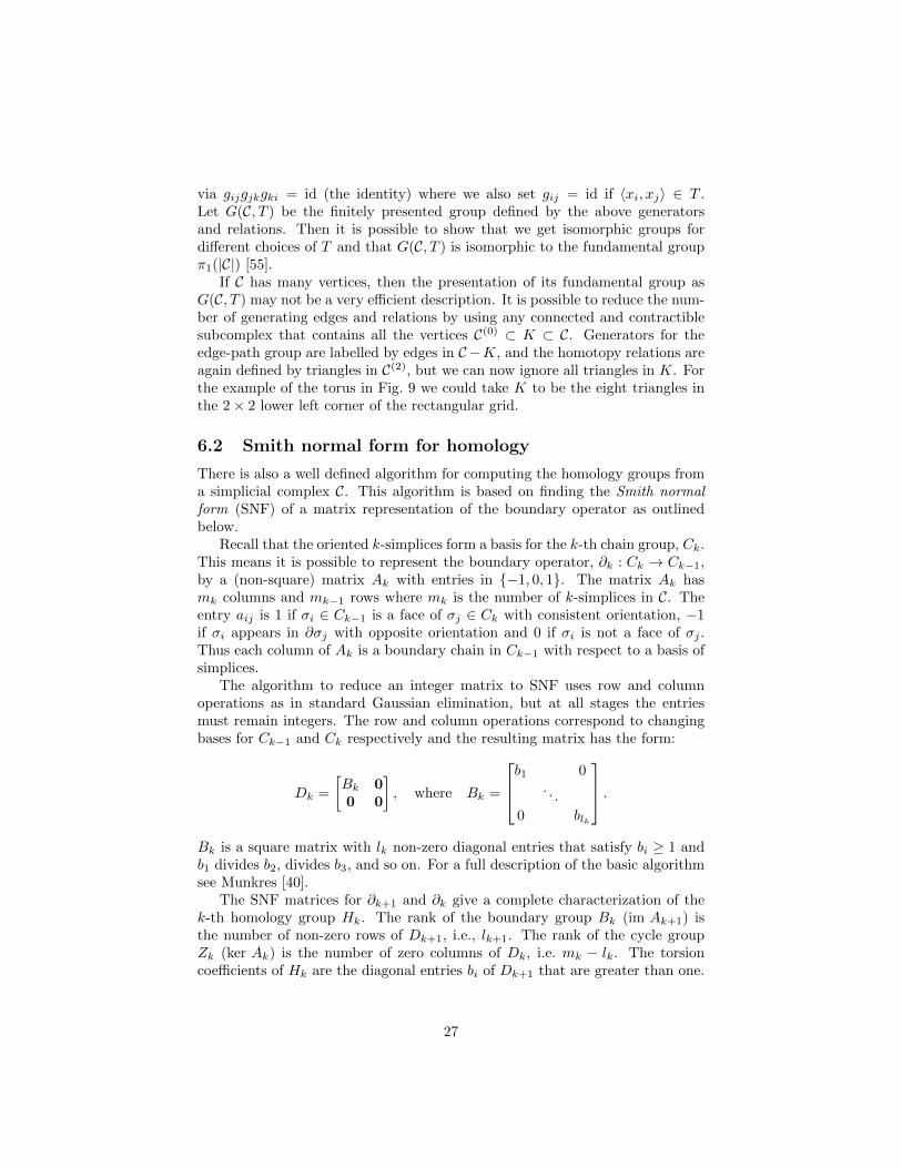
6.2 Smith normal form for homology

There is also a well defined algorithm for computing the homology groups froma simplicial complex C. This algorithm is based on finding the Smith normalform (SNF) of a matrix representation of the boundary operator as outlinedbelow.

Recall that the oriented k-simplices form a basis for the k-th chain group, Ck.This means it is possible to represent the boundary operator, ∂k : Ck → Ck−1,by a (non-square) matrix Ak with entries in −1, 0, 1. The matrix Ak hasmk columns and mk−1 rows where mk is the number of k-simplices in C. Theentry aij is 1 if σi ∈ Ck−1 is a face of σj ∈ Ck with consistent orientation, −1if σi appears in ∂σj with opposite orientation and 0 if σi is not a face of σj .Thus each column of Ak is a boundary chain in Ck−1 with respect to a basis ofsimplices.

The algorithm to reduce an integer matrix to SNF uses row and columnoperations as in standard Gaussian elimination, but at all stages the entriesmust remain integers. The row and column operations correspond to changingbases for Ck−1 and Ck respectively and the resulting matrix has the form:

Dk =

[Bk 00 0

], where Bk =

b1 0. . .

0 blk

.Bk is a square matrix with lk non-zero diagonal entries that satisfy bi ≥ 1 andb1 divides b2, divides b3, and so on. For a full description of the basic algorithmsee Munkres [40].

The SNF matrices for ∂k+1 and ∂k give a complete characterization of thek-th homology group Hk. The rank of the boundary group Bk (im Ak+1) isthe number of non-zero rows of Dk+1, i.e., lk+1. The rank of the cycle groupZk (ker Ak) is the number of zero columns of Dk, i.e. mk − lk. The torsioncoefficients of Hk are the diagonal entries bi of Dk+1 that are greater than one.

27

The kth Betti number is therefore

βk = rank(Zk)− rank(Bk) = mk − lk − lk+1.

Bases for Zk and Bk (and hence Hk) are determined by the row and columnoperations used in the SNF reduction but the cycles found in this way typicallyhave poor geometric properties.

There are two practical problems with the algorithm for reducing a matrixto SNF as it is described in Munkres [40]. First, the time-cost of the algorithmis of a high polynomial degree in the number of simplices; second, the entriesof the intermediate matrices can become extremely large and create numericalproblems, even when the initial matrix and final normal form have small integerentries. When only the Betti numbers are required, it is possible to do better.In fact, if we construct the homology groups over the rationals, rather thanthe integers, then we need only apply Gaussian elimination to diagonalize theboundary operator matrices; doing this means we lose all information about thetorsion however. Devising algorithms that overcome these problems and are fastenough to be effective on large complexes is an area of active research.

6.3 Persistent homology

The concept of persistent homology arose in the late 1990s from attempts toextract meaningful topological information from data [47, 26, 22]. To give afinite set of points some interesting topological structure requires the introduc-tion of a parameter to define which points are connected. The key lesson learntfrom examining data was that rather than attempting to choose a single bestparameter value, it is much more valuable to investigate a range of parametervalues and describe how the topology changes with this parameter. So persistenthomology tracks the topological properties of a sequence of nested spaces calleda filtration · · · ⊂ Ca ⊂ Cb ⊂ · · · where a < b ∈ I is an index parameter. In acontinuous setting, the nested spaces might be the level cuts of a Morse functionon a manifold, so that I is a real interval. In a discrete setting this becomes asequence of subcomplexes indexed by a finite set of integers. In either case asthe filtration grows, topological features appear and may later disappear. Thepersistent homology group, Hk(a, b) measures the topological features fromCa that are still present in Cb. Formally, Hk(a, b) is the image of the map inducedon homology by the simple inclusion of Ca into Cb. Algebraically, it is definedby considering cycles in Ca to be equivalent with respect to the boundaries inCb:

Hk(a, b) = Zk(a)/ (Bk(b) ∩ Zk(a)) .

Computationally, persistent homology tracks the birth and death of everyequivalence class of cycle and provides a complete picture of the topologicalstructure present at all stages of the filtration. The initial algorithm for doingthis, due to Edelsbrunner, Letscher and Zomorodian [22], is surprisingly simpleand rests on the observation that if we build a cell complex by adding a singlecell at each step, then (since all its faces must already be present) this cell either

28

creates a new cycle and is flagged as positive, or ‘fills in’ a cycle that alreadyexisted and is labelled negative. If σ is a negative (k + 1)-cell, its boundary ∂σis a k-cycle and its cells are already flagged as either positive or negative. Thenew cell σ is then paired with the most recently added (i.e. youngest) unpairedpositive cell in ∂σ. If there are no unpaired positive cells available, we mustgrow ∂σ to successively larger homologous cycles until an unpaired positive cellis found. By doing this carefully we can guarantee that σ is paired with thepositive k-cell that created the homology class of ∂σ. Determining whethera cell is positive or negative a priori is computationally non-trivial in generalbut there is a more recent version of the persistence pairing algorithm due toZomorodian and Carlsson [59, 58] that avoids doing this as a separate step, andalso finds a representative k-cycle for each homology class.

The result of computing persistent homology from a finite filtration is alist of pairs of simplices (σ(k), τ (k+1)) that represent the birth and death of eachhomology class in the filtration. The persistence interval for each homology classis then given by the indices at which the creator σ and destroyer τ entered thefiltration. Some non-trivial homology classes may be present at the final step ofthe filtration, these have an empty partner and are assigned ‘infinite’ persistence.There are a number of ways to represent this persistence information graphically:the two most popular techniques are the barcode [11] and the persistence diagram[22]. The barcode has a horizontal axis representing the filtration index; for eachhomology class a solid line spanning the persistence interval is drawn in a stackabove the axis. The persistence diagram plots the (birth, death) index pair foreach cycle. These points lie above the diagonal, and points close to the diagonalare homology classes that have low persistence. It is possible to show thatpersistence diagrams are stable with respect to small perturbations in the data.Specifically, if the filtration is defined by the level cuts of a Morse function on amanifold, then a small perturbation to this function will produce a persistencediagram that is close to that of the original one [13].

6.4 Cell complexes from data

We now address how to build a cell complex and a filtration for use in persistenthomology computations. Naturally, the techniques differ depending on the typeof data being investigated; we discuss some common scenarios below.

The first construction is based on a general technique from topology calledthe nerve of a cover. Suppose we have a collection of ‘good’ sets (the setsand their intersections should be contractible) U = U1, . . . , UN whose union⋃Ui is the space we are interested in. An abstract simplicial complex N (U)

is defined by making each Ui a vertex and adding a k-simplex whenever theintersection Ui0 ∩ · · · ∩ Uik 6= ∅. The nerve lemma states that N (U) has thesame homotopy type as

⋃Ui [28].

If the data set, X, is not too large, and the points are fairly evenly distributedover the object they approximate, it makes sense to choose the Ui to be ballsof radius a centered on each data point: Ua = B(xi, a), xi ∈ X. This is oftencalled the Cech complex; see Fig. 10. If a < b, we see that N (Ua) ⊂ N (Ub),

29

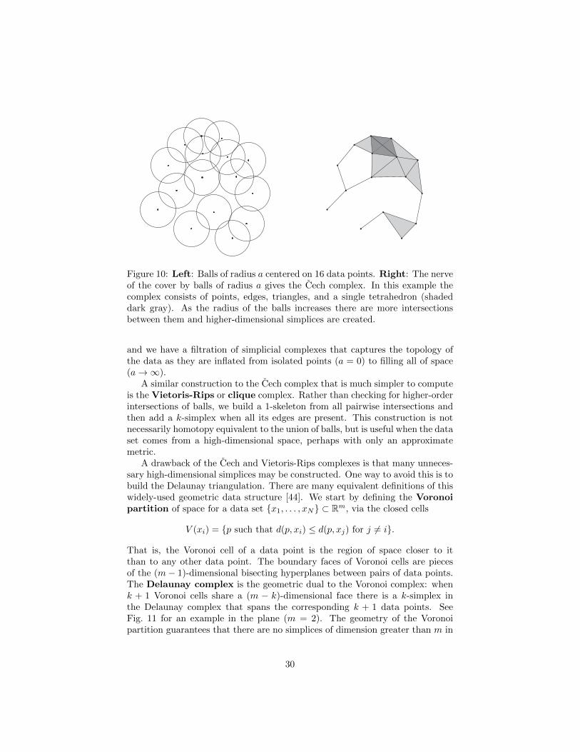
Figure 10: Left: Balls of radius a centered on 16 data points. Right: The nerveof the cover by balls of radius a gives the Cech complex. In this example thecomplex consists of points, edges, triangles, and a single tetrahedron (shadeddark gray). As the radius of the balls increases there are more intersectionsbetween them and higher-dimensional simplices are created.

and we have a filtration of simplicial complexes that captures the topology ofthe data as they are inflated from isolated points (a = 0) to filling all of space(a→∞).

A similar construction to the Cech complex that is much simpler to computeis the Vietoris-Rips or clique complex. Rather than checking for higher-orderintersections of balls, we build a 1-skeleton from all pairwise intersections andthen add a k-simplex when all its edges are present. This construction is notnecessarily homotopy equivalent to the union of balls, but is useful when the dataset comes from a high-dimensional space, perhaps with only an approximatemetric.

A drawback of the Cech and Vietoris-Rips complexes is that many unneces-sary high-dimensional simplices may be constructed. One way to avoid this is tobuild the Delaunay triangulation. There are many equivalent definitions of thiswidely-used geometric data structure [44]. We start by defining the Voronoipartition of space for a data set x1, . . . , xN ⊂ Rm, via the closed cells

V (xi) = p such that d(p, xi) ≤ d(p, xj) for j 6= i.

That is, the Voronoi cell of a data point is the region of space closer to itthan to any other data point. The boundary faces of Voronoi cells are piecesof the (m− 1)-dimensional bisecting hyperplanes between pairs of data points.The Delaunay complex is the geometric dual to the Voronoi complex: whenk + 1 Voronoi cells share a (m − k)-dimensional face there is a k-simplex inthe Delaunay complex that spans the corresponding k + 1 data points. SeeFig. 11 for an example in the plane (m = 2). The geometry of the Voronoipartition guarantees that there are no simplices of dimension greater than m in

30

Figure 11: Left: The Voronoi diagram of a data set with 16 points. Centre:The corresponding Delaunay triangulation. Right: The union of balls of radiusa centred on the data points and partitioned by the Voronoi cells. The corre-sponding triangulation is almost the same as that shown in Fig. 10: instead ofthe tetrahedron there are just two acute triangles.

the Delaunay complex. 7

Now consider what happens when we take the intersection of each Voronoicell with a ball centered on the data point, B(xi, a). The Voronoi cells partitionthe union of balls

⋃B(xi, a) and the geometric dual is a subset of the Delaunay

complex that is commonly referred to as an alpha complex or alpha shape(where alpha refers to the radius of the ball [18, 19]). By increasing the ball ra-dius from zero to some large enough value, we obtain a filtration of the Delaunaycomplex that starts with the finite set of data points and ends with the entireconvex hull. The topology and geometry of alpha complexes has been used,for example, in characterizing the shape of and interactions between proteins[20]. The Betti numbers of alpha shapes are also a useful tool for characterizingstructural patterns of spatial data [45] such as the distribution of galaxies in thecosmic web [57].

When the data set is very large, a dramatic reduction in the number of sim-plices used to build a complex is achieved by defining landmarks and the witnesscomplex. This construction generalises the Voronoi and Delaunay method, sothat only a subset of data points (the landmarks) are used as vertices for thecomplex, whilst still maintaining topological accuracy. A further advantage isthat only the distances between data points are required to determine whetherto include a simplex in the witness complex. See [10] for details, and [12] for anextensive review of applications in data analysis.

Another important class of data is digital images which can be binary(voxels are black or white), greyscale (voxels take a range of discrete values),or coloured (voxels are assigned a multi-dimensional value). In this setting, the

7This is true for points in general position. Degenerate configurations of points occur, forexample in the plane, when four Voronoi cells meet at a point. In this case the Delaunaycomplex may be assigned either a 3-simplex, a quadrilateral cell, or one of two choices oftriangle pairs.

31

structures of interest arise from level cuts of functions defined on a regular grid.Morse theory is the natural tool to apply here, although in this application,the structures of interest are the level cuts of the function while the domain(a rectangular box) is simple. There are a number of different approaches tocomputing homology from such data and this is an area of active research. Theworks [30, 48, 6] present solutions motivated by applications in the physicalsciences.

Guide to further reading

We give a brief precis of a few standard texts on algebraic topology from math-ematical and physical perspectives.

Allen Hatcher’s Algebraic Topology [28] is one of the most widely used texts inmathematics courses today and has a strong geometric emphasis. Munkres’ [40]is an older text that remains popular. Spanier [55] is a dense mathematicalreference and has one of the most complete treatments of the fundamentalsof algebraic topology. A readable introduction to Morse theory is given byMatsumoto [31] and Forman’s review article [24] is an excellent introduction tohis discrete Morse theory.

Textbooks written for physicists that cover algebraic topology include Naka-hara’s comprehensive book Geometry, Topology and Physics [42], Schwarz Topol-ogy for Physicists [50] and Naber Topology, Geometry and Gauge Theory [41].Each book goes well beyond algebraic topology to study its interactions withdifferential geometry and functional analysis. A celebrated example of this isthe Atiyah-Singer index theorem which relates the analytic index of an ellip-tic differential operator on a compact manifold to a topological index of thatmanifold, a result that has been useful in the theoretical physics of fundamentalparticles.

References

[1] P. Alexandroff and H. Hopf. Topologie. Springer, Berlin, 1935.

[2] M.A. Armstrong. Basic Topology. Springer-Verlag, 1983.

[3] C.H. Arns, M.A. Knackstedt, and K.R. Mecke. Reconstructing complexmaterials via effective grain shapes. Physical Review Letters, 91:215506,2003.

[4] Augustin Banyaga and David Hurtubise. Lectures on Morse Homology.Kluwer Academic Publishers, Netherlands, 2004.

[5] Y. Baryshnikov and R. Ghrist. Target enumeration via Euler characteristicintegrals. SIAM Journal of Applied Mathematics, 70(9):825–844, 2009.

32

[6] P. Bendich, H. Edelsbrunner, and M. Kerber. Computing robustness andpersistence for images. IEEE Transactions on Visualization and ComputerGraphics, 16:1251–1260, 2010.

[7] R. Bott. Nondegenerate critical manifolds. Annals of Mathematics,60(2):248–261, 1954.

[8] R. Bott. Morse theory indomitable. Publications Mathematiques deI.H.E.S., 68:99–114, 1988.

[9] R. Bott and L.W. Tu. Differential forms in algebraic topology. Springer,New York, USA, 1982.

[10] G. Carlsson and V. de Silva. Topological estimation using witness com-plexes. In M. Alexa and S. Rusinkiewicz, editors, Eurographics symposiumon point-based graphics, ETH, Zurich, Switzerland, 2004.

[11] G. Carlsson, A. Zomorodian, A. Collins, and L. Guibas. Persistence bar-codes for shapes. International Journal of Shape Modelling, 11:149–187,2005.

[12] Gunnar Carlsson. Topology and data. Bulletin of the American Mathe-matical Society, 46(2):255–308, 2009.

[13] D. Cohen-Steiner, H. Edelsbrunner, and J. Harer. Stability of persistencediagrams. Discrete and Computational Geometry, 37:103–120, 2007.

[14] Charles C. Conley. Isolated invariant sets and the Morse index. Number 38in CBMS. AMS, Providence, Rhode Island, 1978.

[15] Charles C. Conley and Robert Easton. Isolated invariant sets and isolatingblocks. Transactions of the American Mathematical Society, 158:35–61,1971.

[16] J. Curry, R. Ghrist, and M. Robinson. Euler calculus and its applicationsto signals and sensing. In A. Zomorodian, editor, Advances in Applied andComputational Topology, volume 70, pages 75–146, 2012.

[17] Cecil Jose A. Delfinado and Herbert Edelsbrunner. An incremental algo-rithm for Betti numbers of simplicial complexes. In SCG ’93: Proceedingsof the ninth annual symposium on Computational geometry, pages 232–239,New York, 1993. ACM.

[18] H. Edelsbrunner, D.G. Kirkpatrick, and R. Seidel. On the shape of a set ofpoints in the plane. IEEE Transactions on Information Theory, 29(4):551–559, 1983.

[19] H. Edelsbrunner and E.P. Mucke. Three-dimensional alpha shapes. ACMTransactions on Graphics, 13:43–72, 1994.

33

[20] Herbert Edelsbrunner. Biological applications of computational topology.In J.E. Goodman and J. O’Rourke, editors, Handbook of Discrete and Com-putational Geometry, chapter 63, pages 1395–1412. CRC Press, Boca Ra-ton, FL, 2004.

[21] Herbert Edelsbrunner and John Harer. Computational Topology: An intro-duction. American Mathematical Society, Providence, Rhode Island, 2010.

[22] Herbert Edelsbrunner, David Letscher, and Afra Zomorodian. Topologi-cal persistence and simplification. Discrete and Computational Geometry,28:511–533, 2002.

[23] Robin Forman. Morse theory for cell complexes. Advances in Mathematics,134:90–145, 1998.

[24] Robin Forman. A user’s guide to discrete Morse theory. SeminaireLotharingien de Combinatoire, 48, 2002.

[25] G.K. Francis and J.R. Weeks. Conway’s ZIP proof. The American Mathe-matical Monthly, 106(5):393–399, May 1999.

[26] P. Frosini and C. Landi. Size theory as a topological tool for computervision. Pattern Recognition and Image Analysis, 9:596–603, 1999.

[27] P.W. Gross and P.R. Kotiuga. Electromagnetic Theory and Computation:A topological approach. Cambridge University Press, Cambridge, UK.,2004.

[28] Allen Hatcher. Algebraic Topology. Cambridge University Press, Cam-bridge, UK., 2002.

[29] S.T. Hyde, Z. Blum, T. Landh, S. Lidin, B.W. Ninham, S. Andersson, andK. Larsson. The Language of Shape: the role of curvature in condensedmatter. Elsevier, New York, USA, 1996.

[30] Tomasz Kaczynski, Konstantin Mischaikow, and Marian Mrozek. Compu-tational Homology. Springer-Verlag, New York, 2004.

[31] Yukio Matsumoto. An Introduction to Morse Theory, volume 208 of Trans-lations of Mathematical Monographs. AMS, USA, 2002.

[32] Sergei Matveev. Algorithmic topology and classification of 3-manifolds.Springer-Verlag, Berlin, 2003.

[33] Dusa McDuff. Floer theory and low dimensional topology. Bulletin of theAmerican Mathematical Society, 43:25–42, 2005.

[34] Klaus Mecke. Integral geometry in statistical physics. International Journalof Modern Physics B, 12(9):861, 1998.

34

[35] N.D. Mermin. The topological theory of defects in ordered media. Reviewsof Modern Physics, 51:591–648, 1979.

[36] G.B. Mindlin, H.G. Solari, M.A. Natiello, R. Gilmore, and X.-J. Hou. Topo-logical analysis of chaotic time series data from the Belousov-Zhabotinskiireaction. Journal of Nonlinear Science, 1:147–173, 1991.

[37] K. Mischaikow and M. Mrozek. Conley index. In Bernold Fiedler, edi-tor, Handbook of Dynamical Systems, volume 2, chapter 9, pages 393–460.Elsevier, New York, NY, USA, 2002.

[38] M. Morse. The calculus of variations in the large, volume 18 of ColloquiumPublications. American Mathematical Society, Providence, Rhode Island,1934.

[39] M.R. Muldoon, R.S. MacKay, J.P. Huke, and D.S. Broomhead. Topologyfrom a time series. Physica D, 65:1–16, 1993.

[40] James R. Munkres. Elements of Algebraic Topology. Addison-Wesley, Read-ing, MA, 1984.

[41] G. Naber. Topology, Geometry and Gauge fields: Foundations. Springer,Berlin, 2nd edition, 2011.

[42] Mikio Nakahara. Geometry, Topology and Physics. Taylor and Francis, 2ndedition, 2003.

[43] C. Nash and S. Sen. Topology and geometry for physicists. Academic Press,London, UK, 1983.

[44] A. Okabe, B. Boots, K. Sugihara, and S.N. Chiu. Spatial Tessellations:Concepts and Applications of Voronoi Diagrams. John Wiley & Sons,Chichester, 2nd edition, 2000.

[45] V. Robins. Betti number signatures of homogeneous Poisson point pro-cesses. Physical Review E, 74:061107, 2006.

[46] V. Robins, J.D. Meiss, and E. Bradley. Computing connectedness: Anexercise in computational topology. Nonlinearity, 11:913–922, 1998.

[47] Vanessa Robins. Towards computing homology from finite approximations.Topology Proceedings, 24:503–532, 1999.

[48] Vanessa Robins, Peter John Wood, and Adrian P. Sheppard. Theory andalgorithms for constructing discrete Morse complexes from grayscale digitalimages. IEEE Transactions on Pattern Analysis and Machine Intelligence,33(8):1646–1658, 2011.

[49] C. Scholz, F. Wirner, J. Gotz, U. Rue, G.E. Schroder-Turk, K. Mecke, andC. Bechinger. Permeability of porous materials determined from the Eulercharacteristic. Physical Review Letters, 109:264504, 2012.

35

[50] A.S. Schwarz. Topology for Physicists. Springer, Berlin, 2002.

[51] A. Scorpan. The Wild World of 4-Manifolds. American MathematicalSociety, Providence, Rhode Island, 2005.

[52] H. Seifert and W. Threlfall. A Textbook of Topology. Academic Press, 1980.Published in German 1934. Translated by M.A. Goldman.

[53] S. Smale. Generalized Poincare’s conjecture in dimensions greater thanfour. Annals of Mathematics, 74(2):391–406, 1961.

[54] S. Smale. Differentiable dynamical systems. Bulletin of the American Math-ematical Society, 73:747–817, 1967.

[55] Edwin Spanier. Algebraic Topology. Springer, New York, NY, USA, 1994.First published 1966 by McGraw-Hill.

[56] John Stillwell. Mathematics and Its History. Springer, New York, USA,third edition, 2010.

[57] R. van de Weygaert, G. Vegter, H. Edelsbrunner, and et al. Alpha, Bettiand the megaparsec universe: on the topology of the cosmic web. Trans.Comput. Sci., XIV:60–101, 2011.

[58] Afra Zomorodian. Computational topology. In M. Atallah and M. Blan-ton, editors, Algorithms and Theory of Computation Handbook, volume 2Special Topics and Techniques, chapter 3. Chapman & Hall/CRC Press,Boca Raton, FL, second edition, 2009.

[59] Afra Zomorodian and Gunnar Carlsson. Computing persistent homology.Discrete and Computational Geometry, 33:249–274, 2005.

36