algorithms for public decision making
TRANSCRIPT
Algorithms for Public Decision Making
by
Brandon Fain
Department of Computer ScienceDuke University
Date:Approved:
Kamesh Munagala, Supervisor
Vincent Conitzer
Pankaj K. Agarwal
Ashish Goel
Dissertation submitted in partial fulfillment of the requirements for the degree ofDoctor of Philosophy in the Department of Computer Science
in the Graduate School of Duke University2019

Abstract
Algorithms for Public Decision Making
by
Brandon Fain
Department of Computer ScienceDuke University
Date:Approved:
Kamesh Munagala, Supervisor
Vincent Conitzer
Pankaj K. Agarwal
Ashish Goel
An abstract of a dissertation submitted in partial fulfillment of the requirements forthe degree of Doctor of Philosophy in the Department of Computer Science
in the Graduate School of Duke University2019

Copyright © 2019 by Brandon FainAll rights reserved except the rights granted by the
Creative Commons Attribution-Noncommercial Licence

Abstract
In public decision making, we are confronted with the problem of aggregating the
conflicting preferences of many individuals about outcomes that affect the group.
Examples of public decision making include allocating shared public resources and
social choice or voting. We study these problems from the perspective of an algorithm
designer who takes the preferences of the individuals and the constraints of the
decision making problem as input and efficiently computes a solution with provable
guarantees with respect to fairness and welfare, as defined on individual preferences.
Concerning fairness, we develop the theory of group fairness as core or propor-
tionality in the allocation of public goods. The core is a stability based notion
adapted from cooperative game theory, and we show extensive algorithmic connec-
tions between the core solution concept and optimizing the Nash social welfare, the
geometric mean of utilities. We explore applications in public budgeting, multi-issue
voting, memory sharing, and fair clustering in unsupervised machine learning.
Regarding welfare, we extend recent work in implicit utilitarian social choice to
choose approximately optimal public outcomes with respect to underlying cardinal
valuations using limited ordinal information. We propose simple randomized algo-
rithms with strong utilitarian social cost guarantees when the space of outcomes is
metric. We also study many other desirable properties of our algorithms, including
approximating the second moment of utilitarian social cost. We explore applications
in voting for public projects, preference elicitation, and deliberation.
iv

Contents
Abstract iv
Acknowledgements ix
1 Introduction 1
1.1 Fair Resource Allocation Overview . . . . . . . . . . . . . . . . . . . 4
1.2 High Level Survey of Related Work and Applications . . . . . . . . . 7
1.2.1 Fair Allocation. . . . . . . . . . . . . . . . . . . . . . . . . . . 8
1.2.2 Other Related Topics in Computer Science and Economics . . 11
1.3 Outline of Results. . . . . . . . . . . . . . . . . . . . . . . . . . . . . 15
2 Fair Divisible Decisions 19
2.1 Introduction . . . . . . . . . . . . . . . . . . . . . . . . . . . . . . . . 20
2.2 Fairness as Core . . . . . . . . . . . . . . . . . . . . . . . . . . . . . . 21
2.3 Linear Additive Utilities . . . . . . . . . . . . . . . . . . . . . . . . . 24
2.3.1 Application in Memory Sharing . . . . . . . . . . . . . . . . . 25
2.3.2 Mechanism Design . . . . . . . . . . . . . . . . . . . . . . . . 27
2.4 Concave Utilities . . . . . . . . . . . . . . . . . . . . . . . . . . . . . 30
2.4.1 Computing the Lindahl Equilibrium . . . . . . . . . . . . . . . 33
2.5 Conclusion and Open Directions . . . . . . . . . . . . . . . . . . . . . 36
3 Fair Indivisible Decisions 38
3.1 Introduction . . . . . . . . . . . . . . . . . . . . . . . . . . . . . . . . 39
v

3.1.1 Fairness Properties . . . . . . . . . . . . . . . . . . . . . . . . 42
3.1.2 Results . . . . . . . . . . . . . . . . . . . . . . . . . . . . . . . 45
3.1.3 Related Work . . . . . . . . . . . . . . . . . . . . . . . . . . . 47
3.2 Prelude: Nash Social Welfare . . . . . . . . . . . . . . . . . . . . . . 49
3.2.1 Integer Nash Welfare and Smooth Variants . . . . . . . . . . . 50
3.2.2 Fractional Max Nash Welfare Solution . . . . . . . . . . . . . 52
3.3 Matroid Constraints . . . . . . . . . . . . . . . . . . . . . . . . . . . 52
3.4 Matching Constraints . . . . . . . . . . . . . . . . . . . . . . . . . . . 58
3.5 General Packing Constraints . . . . . . . . . . . . . . . . . . . . . . . 62
3.5.1 Result and Proof Idea . . . . . . . . . . . . . . . . . . . . . . 64
3.5.2 Algorithm . . . . . . . . . . . . . . . . . . . . . . . . . . . . . 68
3.5.3 Analysis . . . . . . . . . . . . . . . . . . . . . . . . . . . . . . 69
3.6 Conclusion and Open Directions . . . . . . . . . . . . . . . . . . . . . 76
4 Fair Clustering 78
4.1 Introduction . . . . . . . . . . . . . . . . . . . . . . . . . . . . . . . . 79
4.1.1 Preliminaries and Definition of Proportionality . . . . . . . . . 81
4.1.2 Results and Outline . . . . . . . . . . . . . . . . . . . . . . . . 84
4.1.3 Related Work . . . . . . . . . . . . . . . . . . . . . . . . . . . 85
4.2 Existence and Computation of Proportional Solutions . . . . . . . . . 87
4.3 Proportionality as a Constraint . . . . . . . . . . . . . . . . . . . . . 91
4.4 Sampling for Linear-Time Implementations and Auditing . . . . . . . 94
4.5 Implementations and Empirical Results . . . . . . . . . . . . . . . . . 97
4.5.1 Local Capture Heuristic . . . . . . . . . . . . . . . . . . . . . 97
4.5.2 Proportionality and k-means Objective Tradeoff . . . . . . . . 98
4.6 Conclusion and Open Directions . . . . . . . . . . . . . . . . . . . . . 101
vi

5 Metric Implicit Utilitarian Voting via Bargaining 102
5.1 Introduction . . . . . . . . . . . . . . . . . . . . . . . . . . . . . . . . 103
5.1.1 Background: Bargaining Theory . . . . . . . . . . . . . . . . . 104
5.1.2 A Practical Compromise: Sequential Pairwise Deliberation . . 105
5.1.3 Analytical Model: Median Graphs and Sequential Nash Bar-gaining . . . . . . . . . . . . . . . . . . . . . . . . . . . . . . . 107
5.2 Median Graphs and Nash Bargaining . . . . . . . . . . . . . . . . . . 109
5.3 The Efficiency of Sequential Deliberation . . . . . . . . . . . . . . . . 111
5.3.1 Lower Bounds on Distortion . . . . . . . . . . . . . . . . . . . 115
5.4 Properties of Sequential Deliberation . . . . . . . . . . . . . . . . . . 118
5.5 General Metric Spaces . . . . . . . . . . . . . . . . . . . . . . . . . . 125
5.6 Conclusion and Open Directions . . . . . . . . . . . . . . . . . . . . . 130
6 Metric Implicit Utilitarian Voting with Constant Sample Complex-ity 132
6.1 Introduction . . . . . . . . . . . . . . . . . . . . . . . . . . . . . . . . 133
6.1.1 Results . . . . . . . . . . . . . . . . . . . . . . . . . . . . . . . 134
6.1.2 Related Work . . . . . . . . . . . . . . . . . . . . . . . . . . . 137
6.1.3 Preliminaries . . . . . . . . . . . . . . . . . . . . . . . . . . . 138
6.2 Random Referee and Squared Distortion . . . . . . . . . . . . . . . . 142
6.3 Distortion of Random Referee on the Euclidean Plane . . . . . . . . . 147
6.3.1 Lower Bounds for Distortion in the Restricted Model. . . . . . 147
6.3.2 Upper Bound for Distortion of Random Referee in the Re-stricted Model. . . . . . . . . . . . . . . . . . . . . . . . . . . 151
6.4 Favorite Only Mechanisms: Random Oligarchy . . . . . . . . . . . . . 159
6.5 Conclusion and Open Directions . . . . . . . . . . . . . . . . . . . . . 161
7 Conclusion 164
vii

8 Appendix 168
8.1 Proof of Theorem 2 . . . . . . . . . . . . . . . . . . . . . . . . . . . . 168
8.2 Proof of Theorem 8 . . . . . . . . . . . . . . . . . . . . . . . . . . . . 172
8.3 Proof of Lemma 10 . . . . . . . . . . . . . . . . . . . . . . . . . . . . 174
8.3.1 Step 1: Consolidating Demands . . . . . . . . . . . . . . . . . 175
8.3.2 Step 2: Consolidating Centers . . . . . . . . . . . . . . . . . . 176
8.3.3 Step 3: Rounding an Integer Solution . . . . . . . . . . . . . . 177
Bibliography 178
viii

Acknowledgements
The work represented in this document would have been impossible without the
support of many teachers and mentors. I should especially thank my doctoral adviser
Kamesh Munagala. He had faith in me as a young graduate student that I would only
later develop in myself, and I owe much of my scholarly expertise to him. I admire
his determination to seek and work on problems that are interesting and relevant in
society as well as the scholarly community, and to emphasize constructive algorithmic
approaches that prefer simplicity.
Debmalya Panigrahi, Pankaj Agarwal, Vincent Conitzer, and Rong Ge were all
important teachers in my graduate education at Duke; I am indebted to them for my
training as a computer scientist. Rong taught me much about algorithms for machine
learning and optimization. From Vincent, I learned a great deal about algorithmic
game theory, mechanism design, and computational social choice. Pankaj was my
first and very excellent teacher of algorithms in graduate school. In addition to
teaching approximation and graph algorithms, Debmalya has always provided clear
and useful feedback. I should also note that I had the privilege of teaching with
Carlo Tomasi, John Reif, Ashwin Machanavajjhala, and Xi He, and that teaching
with these individuals formed me just as significantly as the classes I myself took
from others.
I have also been fortunate to have many wonderful collaborators in my research
over the years. In addition to my adviser, these collaborators include Ashish Goel,
ix

Nisarg Shah, Nina Prabhu, Xingyu Chen, Liang Lyu, and Mayuresh Kunjir. Mayuresh
was a more senior graduate student who worked graciously with me on my first re-
search project during my first year of graduate school. Xingyu and Liang are both
undergraduates at Duke who worked diligently despite their academic obligations,
and I am grateful for having had the opportunity to mentor and assist them. Nina
was a high school senior at the North Carolina School of Science and Math when she
began working on a project with me, and is now an undergraduate computer science
student at Stanford. Nisarg Shah was finishing his PhD at Carnegie Mellon when
we met, and is now a professor at the University of Toronto. We have many shared
interests in research, and talking with Nisarg has always encouraged me about the
possibilities of our work, as well as clarified the problems at hand. Ashish was been
deeply involved in establishing many of the fundamental questions in this disserta-
tion as research interests for me (namely participatory budgeting and deliberation),
and brings a rich breadth of experience to these issues that spans theory and prac-
tice. The contributions of these collaborators to specific chapters are noted at the
beginning of each chapter.
A dissertation requires more than intellectual support. Marilyn Butler deserves
special thanks for her role in supporting me as a staff person through the entire pro-
gram from admission to graduation. I must also thank my family, the other students
in the computer science department at Duke, the Graduate Christian Fellowship at
Duke, Blacknall Presbyterian Church, and especially Seaver Wang and Olivia Brown
for forming the community that grounded, supported, and encouraged me. The ideas
of these individuals and communities are not present in this dissertation, but it would
surely have been impossible without them.
Finally, my work was financially supported by Duke University and by NSF grants
CCF-1408784, CCF-1637397, and IIS-1447554.
x

1
Introduction
“If a house is divided against itself, that house cannot stand.”1
Any collection of individuals seeking to work together must make decisions that
affect the whole, even when they disagree about the right decision. This tension is
endemic to all modes of human society, and is increasingly relevant to collections
of artificially intelligent agents as well as automated algorithmic decision making
via machine learning. In this thesis, I design and analyze principled algorithms for
making these kinds of public decisions.
There are many aspects to public decision making. The processes by which we
come to decisions are deeply rooted in traditions and institutions. The individuals
involved in decision making may be complex human beings with desires, anxieties,
relationships, fears, and hopes. While I do not intend to dispute the significance
of these aspects of lived decision-making, I do wish to suggest that there are deep
problems in addition to these historical, emotional, and social concerns. The aspects
of public decision making I consider in this thesis are normative and algorithmic
1 Jesus of Nazareth according to the Gospel of Mark
1

in nature: even if we could somehow cleanly separate out the preferences of the
individual agents, how should we aggregate those preferences into a single decision,
and how would we justify our procedure in terms of those preferences?
I will tend to consider problems as follows. We will have a set of agents and a set of
possible outcomes. Feasible outcomes may be constrained in some way. For example,
perhaps we only have so many dollars to spend. Agents will have preferences over
possible outcomes, and we will generally represent these preferences as utilities.2 We
will design efficient algorithms that take as input the preferences of the agents, and
output a feasible outcome that provides some provable guarantee in terms of the
preferences of the agents. In so doing, we will develop principled solutions for public
decision making.
This thesis considers two broad approaches. In the first chapters, we will consider
fair resource allocation of public goods. Here, we consider guarantees that fairly
respect the relative entitlements of the agents, ensuring that no group of agents
is poorly treated. More specifically, we adapt a game theoretic notion of stability
called the core as a novel fair solution concept in public decision making or public
resource allocation. Subsequently, we study the computation of core solutions under a
variety of settings including divisible and indivisible public goods, linear and concave
utilities, and metric centroid clustering. Along the way, we consider applications in
public budgeting, voting, memory sharing, and fair machine learning. Resource
allocation is a fundamental problem in economics and computer science, but most of
2 The use of the word “utility” connotes many things to many people. In the philosophicaltradition, it may indicate a historically Anglo-American approach to ethics. I will generally useutilities to quantify the benefit an individual derives from a particular outcome of public decisionmaking. I am not ideologically committed to the notion that an individual is ethical in so far asshe makes decisions that maximize the arithmetic mean of societal utilities. Also, the fact thatI generally think of utilities as quantifying the benefit to an individual of an outcome does notimply that I assume the agents are selfish or malicious. If one prefers, one can think of utilities asquantifying the extent to which an agent perceives a given outcome as good in the broad sense. Inso far as agents disagree, deep problems remain.
2

the prior work in the fair resource allocation literature focused on private goods, for
which the solution concepts tend to be either ill-defined or too-weak when considering
public goods. Nevertheless, we find interesting connections with prior and ongoing
work in terms of our algorithmic approaches, some of which are based on the Nash
social welfare function.
In the second part of the thesis, we consider public decision making as social
choice. We study making a single public decision in the implicit utilitarian model
where we want to minimize the utilitarian social cost but we only know ordinal pref-
erences of agents (i.e., we are not given utilities, only rankings over outcomes). We
design simple randomized mechanisms that approximately minimize the utilitarian
social cost when the space of possible outcomes forms a metric. We extend prior
work in this setting by providing mechanisms that have additional desirable proper-
ties like approximating the second moment of the distribution of social cost (where
the randomness comes from the randomization in the mechanism) and using only a
constant number of queries.
Though our treatment will often be mathematical and necessarily abstract, the
broad problem I have outlined is not. Americans are often prone to wonder whether
conducting presidential elections by the popular vote or the electoral college would be
better. Every year, tax dollars are allocated at the federal, state, and local levels to
fund public projects and resources. Algorithms and machine learning are increasingly
used for making public decisions about granting loans and bail, matching employers
and employers, school admissions, and more. The average family or group of friends
may be familiar with the inscrutable difficulties of agreeing on a place to eat dinner.
Public decisions are made one way or another, and through mathematical analysis,
we can hopefully come to see the tradeoffs more clearly across diverse scenarios.
It is important to clarify at the outset that my goal is constructive, not descriptive
or rhetorical. I seek to provide clean and precise abstract descriptions of problems in
3

public decision making, to present reasonable and precise notions of a good solution,
and to provide efficient algorithms for constructing such solutions. I will not answer
two other extremely interesting kinds of questions. First, I will not consider the
development of a broad theory of justice from which particular statements of rights
or entitlements may be derived. While I argue for the reasonableness of various
normative guarantees in this thesis, I make no attempt to justify them as necessary.
Second, I will not consider the normative question for individuals. That is, I will
not ask questions of the sort “what should some particular agent do when engaged
in making a public decision?” I will always take the normative perspective with
respect to the mediator or designer of a mechanism, and only ever assume strategic
or sincere behavior on the part of agents.
1.1 Fair Resource Allocation Overview
In this section, I describe some of the most important concepts in the area of fair
resource allocation in general terms as a reference and a gentle introduction that will
relate to our discussion of both fair resource allocation for public goods and implicit
utilitarian social choice. Individual chapters further refine notation and definitions
for specific applications; this introduction is intended to clarify something of the
breadth of possible models for related problems. In particular, many of these notions
are stated for private goods as is standard practice, and we will need to slightly adapt
the notions for public goods.
A setting (or model) for a fair resource allocation problem consists of a set N of
|N | “ n agents and a set M of |M | “ m goods. If the goods are divisible then an
allocation is constituted by values xij P Rě0 for every agent i P N and good j P M
denoting the amount of good j that agent i receives. If the goods are indivisible then
an allocation is a partition X “ tX1, ..., Xnu such that for all i P N , Xi Ď M , and
for all i, i1 P N such that i ‰ i1, Xi XXi1 “ H.
4

Denote the set of generic (divisible or indivisible) feasible allocations as Y pMq.
An agent has ordinal preferences if she has a complete and transitive ordering ľi
over Y pMq where y1 ľi y2 for y1, y2 P Y pMq should be read as “agent i weakly
prefers allocation y1 to allocation y2.” An agent has cardinal preferences if she has
ordinal preferences and a utility function ui : Y pMq Ñ R satisfying uipy1q ě uipy2q if
and only if y1 ľi y2. In my work, I generally focus on cardinal preferences. Finally,
a good is private if it can be allocated to at most one agent, i.e., all other agents
receive 0 utility from the good. A good is public if it is allocated generally such that
every agent may receive nonzero utility from the good.
Given a specific model, a typical fair allocation problem defines an objective or
certain desiderata that constitute a “good” allocation and proceeds to devise an
algorithm that optimizes that objective or satisfies those desiderata. Some of the
most standard objectives are called social welfare functions, which are functions of
the utilities of the agents (note that such functions are only well defined for cardinal
preferences). Let u P Rn be a vector of the utilities of agents. The three most
common social welfare functions are defined below.
• The utilitarian social welfare (USW) is defined as
USW puq “1
n
ÿ
iPN
ui.
Informally, maximizing the utilitarian social welfare provides “the greatest good
for the greatest number” and maximizes the efficiency of an allocation.
• The Nash social welfare (NSW) is defined as
NSW puq “
˜
ź
iPN
ui
¸1n
.
5

Informally, maximizing the Nash social welfare balances the efficiency and the
fairness of an allocation.
• The egalitarian social welfare (ESW) is defined as
ESW puq “ miniPN
ui.
Informally, maximizing the egalitarian social welfare provides the most good
possible for the worst off individual, and is typically considered the strictest
fairness objective among social welfare functions.
Much of the fair allocation literature attempts to guarantee certain desiderata,
rather than maximize an objective function. We list some common guarantees. Let
yi be the generic allocation to agent i.
• Envy-Freeness. An allocation is envy-free if for all i, i1 P N, yi ľi yi1 .
• Proportionality. An allocation is proportional if for all i P N, uipyiq ěuipMqn
.
• Pareto efficiency or Pareto optimality. A generic allocation y P Y pMq is Pareto
efficient or Pareto optimal if there does not exist another feasible allocation
z P Y pMq such that z ľi y for all i P N and z ąi1 y for some i1 P N (where
z ąi1 y means z ľi1 y but y ńi1 z).3
Finally, the following concepts are the most important for analyzing the strategic
behavior of rational agents. Suppose that we want to design an algorithm or mecha-
nism4 for fair allocation, Ap¨q, and we elicit information in the form of a type vector
3 Note that while Pareto efficiency is a weak notion of efficiency, it can be nontrivial to combinewith envy-freeness or proportionality.
4 Some authors distinguish between an algorithm and a mechanism. Those who do typically usemechanism for algorithms that specifically account for strategic behavior. In generally, I do not makethis distinction, and use algorithm, protocol, and mechanism interchangeably and synonymously inmost contexts.
6

t. Every agent i P N has a true type τi (typically these types will be some form of
utility information for different outcomes) and reports a type ti (not necessarily equal
to τi) to the mechanism. Let t´i be the reported types of all agents apart from agent
i. Let uipτi, Aptqq be agent i’s utility given their true type τi under the outcome of
the mechanism given type vector t (or the expected utility if Ap¨q is randomized).
• Truthfulness. Ap¨q is truthful or strategyproof or dominant-strategy incentive-
compatible if @i P N , @τi, and @t, uipτi, Apτi, t´iqq ě uipτi, Aptqq. Informally,
if a mechanism is truthful, no agent has an incentive to misreport their type
regardless of the reports of the other agents.
• Truthful Equilibrium. Ap¨q has truth telling as a Nash equilibrium (also called
ex-post equilibrium) if @i P N , all agents reporting τi and receiving payoff
uipτi, Apτ1, . . . , τnqq is a Nash equilibrium. Informally, a mechanism has truth
telling as a Nash equilibrium if no agent has an incentive to misreport their
type, assuming no other agents are misreporting their types.
1.2 High Level Survey of Related Work and Applications
An application to which we will repeatedly return is called participatory budgeting [1].
In many cities around the world, a certain amount of public tax money is allocated
directly according to votes elicited from citizens. Some other canonical examples of
fair division like splitting taxi fare, splitting rent [73], and dividing up indivisible
goods have been implemented in software by a recent web deployment http://www.
spliddit.org/. Fair allocation algorithms have also been deployed for allocating
course slots to students [37]. A significantly scaled up application of fair resource
allocation in recent years is the allocation of resources in a datacenter environment
(historically, fairness was of little concern and efficiency was obviously the right
objective for these kinds of problems, but now data centers are often populated with
7

tasks from different users with priorities and rights). For examples, see [76, 139, 100,
135, 72].
1.2.1 Fair Allocation.
A comprehensive technical survey of the fair allocation (also known as fair division)
literature would require its own book, as the field has matured substantially over the
last two decades, bringing together substantial contributions from computer science
and economics. Rather than attempting such a Herculean task, it is my intent in this
section to provide the reader with a high level overview of some of the topics that
are most related to this thesis. Individual chapters will provide additional related
work that is specific to and relevant for the content of the chapter. The interested
reader can also find a survey of topics in fair resource allocation in Part 2 of [34].
Cake Cutting. The canonical problem of fairly allocating divisible private goods is
called cake cutting. The model is usually described by an interval r0, 1s over which
n agents have some utility function. The problem was outlined in a survey by
Ariel Procaccia in 2013 [141]. Generally, one seeks an algorithm within a discrete
query model for computing an envy-free allocation. For two agents, this is always
possible and the algorithm is trivial: ask one agent to cut the “cake” into two pieces
such that each has equal value; ask the second agent to choose among these two
pieces. For three agents, a slightly less trivial algorithm has been known, but a
recent breakthrough showed (i) a discrete envy-free protocol for 4 agents [19] and
(ii) a discrete envy-free protocol for n agents [18].
Heterogeneous Resources. The fair allocation problem may become substantially more
complicated when users have non-additive demands over multiple heterogeneous
goods. This case has been highlighted in the context of algorithms for resource
8

allocation in data centers [76, 139, 100, 135], where the utility jobs receive for mem-
ory, processor time, and bandwidth interact in a way typically described by Leontief
preferences, rather than additive. The crucial idea behind the breakthrough work
of dominant resource fairness [76] is to consider fairness with respect to dominant
resources, which one can think of as the bottleneck resource for a given job.
Integral Allocations: Envy-freeness. Fair allocation also becomes more difficult in the
case where the goods are integral, in the sense that they cannot be fractionally al-
located to the agents. In this context, it is straightforward to see that an envy-free
allocation is not always possible: simply consider the case where there is a single
good and two agents who desire it.5 For this reason, there is an extensive hierarchy
of fair solution concepts developed in the literature. The most straightforward relax-
ation of envy-freeness is envy-freeness up to one good, which says that an allocation
would be envy-free if, for every pair of agents, we considered removing one good
from the allocation to the envied agent. Such solutions always exist for monotone
utility functions [119], and in the special case of additive utility, finding the integral
allocation that maximizes the Nash social welfare satisfies the property [41] and is
also Pareto efficient. Unfortunately, finding the integral allocation that maximizes
the Nash social welfare is APX-hard [115], although constant factor approximation
algorithms are known [50, 49, 6, 24].
A solution concept that lies between envy-freeness and envy-freeness up to one
good is called envy-freeness up to any good. Such a solution would be envy-free
if, for every pair of agents, we considered removing any good of the envied agent.
5 This assumes, of course, some minimal efficiency guarantee such as we must allocate all of thegoods or slightly stronger, Pareto optimality. Also, envy-freeness in expectation is still achievablewith a randomized mechanism, but such solutions are often unsatisfactory in the context of fairdivision, as we are often performing a single allocation of goods that may not be repeated. Forexample, we might be dividing goods among inheritors of an estate. For this reason, the literaturetends to focus on ex-post or deterministic guarantees, rather than guarantees in expectation.
9

The leximin solution, which maximizes the egalitarian social welfare and breaks ties
lexicographically by the least, second least, and so forth utility, computes an envy-
free up to any good solution for two agents [136]. Existence for more agents remains
an open question.
Integral Allocations: Maximin Share Guarantee. Another extensively studied solution
concept is the maximin share guarantee, which was introduced by Budish in [37]
along with the notion of approximate competitive equilibrium from equal incomes.
The maximin share of an agent is the utility they would receive from their least
favorite bundle of goods under the partition of the goods into n bundles that max-
imizes their utility from that least favorite bundle. Procaccia and Wang initiated
the computational study of maximin share guarantees [143], which has since seen
extensive follow up work in the literature [23, 5, 77]. The state of the art is that a
34-multiplicative approximation to the maximin share guarantee always exists and
can be efficiently computed for additive valuations. For submodular valuations, the
best known approximation factor is 13.
Fair Allocation of Public Goods. As we will argue in this thesis, allocating private
goods is a special case of the more general problem of allocating public goods. There-
fore, while solution concepts for public goods do translate to the private goods case,
the converse is not necessarily true, and new approaches are necessary. In particular,
public goods can be shared, and traditional fair solution concepts for private goods
do not take this into account. Instead, we advocate for considering group fairness
that considers guarantees to more general subsets of agents than just singleton indi-
viduals. In addition to our own work, such group guarantees have been considered in
many contexts, including private goods allocation [22, 54] and multi-winner approval
voting in social choice [16, 149].
10

1.2.2 Other Related Topics in Computer Science and Economics
Our treatment will necessarily involve some tools and techniques from outside of the
fair allocation literature itself, and in this section I briefly survey some of the more
relevant such topics at a high level. Again, individual chapters will provide citations
for any references necessary for the chapter.
Market Equilibrium. The culmination of neoclassical economic theory is Walrasian
market equilibrium [99]. Traditionally, economists have been interested in the ex-
istence and properties of equilibrium. More recently however, computer scientists
have become interested in the computability of equilibrium, showing both hard-
ness [158, 44] and efficient methods [98, 97]. This study is partially motivated by
wanting to understand market dynamics: if an equilibrium is computationally hard
to compute, should we expect it to be reached under simple dynamics? However,
there is also interest in computing a market equilibrium outright for other appli-
cations in fair allocation, where the “money” in the market is virtual. The most
common example is a market based notion of fairness called competitive equilibrium
from equal incomes [37] where the idea is that an allocation is fair if it is a market
equilibrium computed from agents with equal incomes. Fisher market equilibrium
proved invaluable in the analysis that Cole and Gkatzelis provided of an algorithm
to approximately maximize the Nash social welfare for indivisible goods [50]. We
crucially use a line of work developed for public goods equilibrium, called the Lin-
dahl equilibrium [118, 101, 71], to compute fair allocations of public goods subject
to a budget constraint in Chapter 2.
Game Theory and Bargaining. Game theory is a normative study of how rational and
self-interested (or strategic) agents should behave in a situation where the actions of
the agents determine the payoffs, or utilities, the players receive. The fundamental
11

solution concept for noncooperative games (those in which the players cannot co-
ordinate their actions) is the Nash equilibrium: a state such that no agent has an
incentive to change their action given the actions of the other agents. A fundamental
computational result in algorithmic game theory is the proof that computing a Nash
equilibrium is a hard problem, more specifically, it is the canonical problem for the
PPAD complexity class (polynomial parity arguments on directed graphs) [58].
Cooperative game theory studies situations where the agents can coordinate
their behavior; a canonical problem with two agents is the bargaining problem, first
phrased in game theoretic terms by Nash [130], who showed that under a set of four
axioms, the Nash social welfare maximizer is the unique solution to such a game.
Rubenstein provided additional justification for Nash’s solution to the bargaining
problem by giving a mechanism that implements the solution as a Nash equilibrium
in a noncooperative game [146]. We use Nash’s solution concept extensively in Chap-
ter 5. Kalai and Smorodinsky provided alternative solution concepts under related
sets of axioms [104, 103]. The study of the bargaining problem has also led to an
attempt to justify the use of cardinal valuations [154, 89]. Myerson expanded the
model to account for incomplete information [128]. A stronger solution concept that
we consider extensively in Chapter 2 is the core, first expounded in game theoretic
terms by Scarf [150]. Informally, an outcome is in the core if no subset of agents can
deviate and select for themselves a preferable outcome. Scarf provides sufficient, but
not necessary, conditions for the existence of the core.
Mechanism Design. Mechanism design attempts to create functions or rules for al-
location problems where the agents who report information to the algorithm have
preferences over the outcomes of the algorithm and must be incentivized to pro-
vide correct information. Two classic notions of such incentives are truthfulness
and Nash equilibrium, described in Section 1.1. Designing truthful mechanisms is
12

often difficult. Two classic impossibility results include the Gibbard-Satterthwaite
impossibility theorem for truthful social choice with ordinal valuations [78] and the
Myerson-Satterthwaite impossibility theorem for truthful bilateral trade [129]. As
a more recent example, Cole et. al examine the fair allocation of divisible private
goods in a strategyproof context without money [51]. They design an algorithm
that, for every agent, provides at least a 1/e fraction of the utility they would have
received under the proportionally fair allocation, while being strategyproof, but they
also provide a 1/2 upper bound for the same problem.
There are, however, several novel techniques and approaches. In 2007, McSh-
erry and Talwar presented the exponential mechanism, a way to use differential pri-
vacy to construct approximately truthful randomized mechanisms for optimization
problems [93]. We use this technique in Chapter 2. In 2013, Cai, Daskalakis, and
Weinberg provided a black box reduction from designing Bayesian incentive com-
patible, ex post individually rational, arbitrarily feasibility constrained mechanisms
optimizing arbitrary objectives to algorithm design for the underlying optimization
plus virtual revenue and virtual welfare [39]. Subsequently, they expanded the work
to include ex-post constraints [57]. A separate approach to mechanism design con-
siders showing that the incentive to misreport often (though not always) diminishes
in large games or large markets. Azevedo and Budish defined the notion of strat-
egyproofness in the large along these lines [14] and Feldman et. al showed how to
bound the Price of Anarchy (a notion of the worst case quality of Nash equilibrium
introduced in [109]) in large games [68].
Utilitarian Social Choice. Informally, social choice theory studies how to pick a point
from a decision space that represents the common good of society. The canonical ex-
ample is voting. In that case, the decision space is usually a small set of candidates,
and the agents comprising the society express only ordinal valuations over these can-
13
didates. Typically, social choice is studied under ordinal preferences, despite the clas-
sic impossibility result from Arrow [11]. In utilitarian social choice, we assume that
agents have cardinal valuations (i.e., utility functions) over the possible decisions.
Some recent work in this area takes an implicit utilitarian perspective, assuming
that agents cannot report their full utility functions but that their reported ordinal
valuations are generated by an underlying cardinal utility function [31, 7, 25, 46].
Such work tries to bound the distortion, the worst case utilitarian social welfare over
all utility functions that could have generated the ordinal reports of agents. Our
work in Chapter 5 and Chapter 6 is in this model.
Much of utilitarian social choice focuses on specific structures for the decision
space and the utilities agents have over it. For combinatorially structured decision
spaces, there is a long line of work [151, 134, 36, 60] on combinatorial public projects.
These results focus on truthful mechanism design and the winner determination prob-
lem. There is ongoing related work on candidate selection even for simple analytical
models like points in R [67]. Median graphs and their ordinal generalization, median
spaces, have been extensively studied in the context of social choice. The special
cases of trees and grids have been examined as structured models for voter prefer-
ences [153, 21]. For general median spaces, it is known that the Condorcet winner
(that is an alternative that pairwise beats any other alternative in terms of voter
preferences) is strongly related to the generalized median [20, 147, 159] – if the for-
mer exists, it coincides with the latter. [132] shows that any single-peaked domain
which admits a non-dictatorial and neutral strategy-proof social choice function is
a median space. [48] also showed that any set of voters and alternatives on a me-
dian graph will have a Condorcet winner. In a sense, these are the largest class of
structured and spatial preferences where ordinal voting over alternatives leads to a
“clear winner” even by pairwise comparisons. Goel and Lee [82] recently worked with
median graphs in devising a sequential process for reaching concsensus. We follow
14
up on these ideas with our work in Chapter 5.
The notion of democratic equilibrium [75] considers social choice mechanisms in
continuous spaces where individual agents with complex utility functions perform
update steps inspired by gradient descent, instead of ordinal voting on the entire
space. Several works have considered iterative voting where the current alternative
is put to vote against one proposed by different random agent chosen each step [4,
116, 144], or other related schemes [124]. The analysis tends to focus on convergence
to an equilibrium instead of welfare or efficiency guarantees.
Textbooks and References. The now classic text on applications of game theory within
an algorithmic context is [133]. A recent book on computational social choice serves
as an excellent survey and reference [34]. My preferred text on approximation algo-
rithms is [160]. I have found [117] useful in the study of Markov chains, and [10] for
its analysis of the multiplicative weights method. My favorite book on game theory
is an old one by John Harsanyi [88], but I have also used the more recent book by
Yoav Shoham and Kevin Leyton-Brown [155].
1.3 Outline of Results.
Chapter 2. In this chapter, we introduce the fair participatory budgeting problem
as a canonical example of public decision making. There are multiple public projects
that we can fund subject to a budget constraint. We introduce the notion of the
core from cooperative game theory as a fair solution concept that generalizes the
idea of proportionality to all subsets of agents. We show that for additive and
linear utility, maximizing the Nash social welfare is a core solution. This can be
implemented efficiently as the Proportional Fairness convex program, and we briefly
discuss application to memory allocation. We go on to show that we can adapt the
exponential mechanism from differential privacy to design an approximately truthful
15

mechanism for computing approximately core solutions with high probability. We
then generalize the class of utility functions under consideration, and show that we
can still compute core solutions via a generalization of the Proportional Fairness
program for a fairly broad class of separable concave utility functions.
Chapter 3. Here, we consider the problem of public decision making where the out-
comes must be chosen integrally and deterministically. We use a broad model that
generalizes much of the prior literature for indivisible fair allocation: there is a set
of public goods, from which we must choose a feasible subset. We work with ad-
ditive valuations, and our results are differentiated based on the type of feasibility
constraints that can be imposed.
It is easy to see that core solutions and their multiplicative approximations may
not exist for integral allocations. Nevertheless, for matroid and matching constraints,
we show that any local maximum of a smoothed version of the Nash social welfare
function is a constant approximate additive core solution, and that such local max-
ima can be efficiently computed via local search techniques. The matroid setting is
sufficient to model the problem where there are a number of binary issues, and we
must choose yes or no for each (i.e., multiple simultaneous referendums). Matroid
constraints are also sufficient to model the multi-winner election problem, where
there are some number of candidates, and we want to elect some subset of the can-
didates of constrained size (also known as committee selection). For general packing
constraints, where each good has an associated multi-dimensional cost, and feasibility
is defined by packing constraints on these costs, we show that the previous approach
is inadequate. Instead, we compute the fractional maximum Nash social welfare so-
lution and a certain maximally fair fractional solution that we define. We mix these
fractional solutions and design a hierarchical rounding algorithm that yields a nearly
logarithmic additive approximate core solution in polynomial time.
16

Chapter 4. In this chapter, we consider centroid clustering as a problem in public
decision making. In particular, we suppose that the data points to be clustered are
individuals who prefer to be accurately clustered, in terms of small distance to their
center in some metric space. We adapt the notion of core in this context and call it
proportional clustering. We note that traditional approaches to clustering like opti-
mizing the k-median, k-means, and k-center objectives need not produce proportional
clusterings, and indeed, exactly proportional clusterings may not exist. Neverthe-
less, we give a greedy algorithm for efficiently computing a constant approximate
proportional clustering. Furthermore, we formulate approximate proportionality as
a linear constraint, and show how to adapt rounding techniques to approximately
minimize the k-median objective subject to proportionality as a constraint. We show
that proportionality is approximately preserved under random sampling, and that
this idea can be used to more efficiently compute and audit proportional clustering
solutions. Finally, we consider the empirical tradeoff between proportionality and
the k-means objective on real data sets.
Chapter 5. This begins the second part of this thesis, wherein we consider implicit
utilitarian social choice. We suppose that we want to choose a single outcome from
a set of alternatives so as to minimize the utilitarian social cost, but we do not know
the costs of the agents for the alternatives. We design a randomized sequential de-
liberation protocol based on iterative Nash bargaining and show that it has expected
social cost within a constant factor of the social optimum when the space of alter-
natives are metric (that is, when costs satisfy the triangle inequality). Furthermore,
we show that the second moment of social cost is also within a constant factor of the
squared social cost of the social optimum. We call this concept of approximation on
the second moment of cost Squared Distortion, and interpret it as a quantification
of the risk associated with a randomized mechanism. We show stronger results (in
17

terms of approximation of the social optimum, but also uniqueness of stationary dis-
tribution, Pareto efficiency, and Nash equilibria) in the special case where the space
of alternatives lie on a median graph, which can be thought of as graphs or metric
spaces that embed isometrically into hypercubes (potentially of high dimension).
Chapter 6. In this chapter, we continue working in the implicit utilitarian model
of social choice using randomized mechanisms when the space of alternatives forms
a metric. However, in this chapter we propose a simple query model and study
mechanisms that are constrained to make a constant number of queries, motivated
by the practical concerns of social choice in very large spaces of alternatives where
lightweight mechanisms are desirable. We show that any mechanism that only queries
about the top-k preferred alternatives of agents (for constant k) must necessarily have
Squared Distortion that scales linearly with the number of agents. On the positive
side, we design a simple mechanism we call Random Referee that incorporates a
single comparison query, and just three queries in total, to obtain constant Squared
Distortion, which also implies that the expected social cost is within a constant fac-
tor of the social optimum. We also show that Random Referee has better expected
social cost in the worst case than any mechanism that only considers top-k preferred
alternatives when the space of alternatives are embedded in the Euclidean plane. Fi-
nally, among mechanisms constrained to only consider the top preferences of agents,
we give a mechanism called Random Oligarchy that is essentially best in class with
respect to the expected social cost.
18

2
Fair Divisible Decisions
In this chapter, we introduce the problem of fair resource allocation for public goods,
the general focus of the first part of this thesis. We begin by considering the problem
of fairly allocating divisible public goods subject to a budget constraint, with the
motivating application of participatory budgeting. We introduce the general prob-
lem, and discuss possible solution concepts. Ultimately, we argue that the core, a
stability condition from cooperative game theory, can be interpreted as a fairness
condition for the allocation of public goods by enforcing proportionality for all sub-
sets of agents. We subsequently show how to compute core allocations by maximizing
the Nash social welfare, when agents have linear and additive utilities. We describe
an application in memory sharing, and show how to adapt the exponential mecha-
nism from differential privacy to construct an approximately truthful mechanism for
computing approximate core solution. Finally, we design a novel convex program
for computing core allocations when agents have a more general class of utility func-
tions that are separable and concave. This allows us to use concave utility functions
to encode soft budget caps on public goods, which is important for our motivating
problem of participatory budgeting.
19

Acknowledgements. These results are published in [63], which is joint work with
Kamesh Munagala and Ashish Goel. The discussion of memory sharing in Sec-
tion 2.3.1 draws on work published in [113], which is joint work with Mayuresh
Kunjir, Kamesh Munagala, and Shivnath Babu.
2.1 Introduction
Classical fair resource allocation tends to focus on private goods. For example, one
can imagine that we have a cake that can be cut into pieces and then allocated to
agents, who perhaps have different utilities for different portions of the cake. In
classical economic theory, a fair allocation is one that is Pareto-efficient and envy-
free [157], meaning that there is no other way to divide up the cake that all agents
prefer, and that no agent prefers the portion of cake allocated to any other agent.
In contrast, we focus on public goods. For example, one can think of shared
resources like roads or parks. Economically, public goods can be characterized as
having positive externalities. We will tend to view public goods as those that can
grant utility to more than one agent simultaneously. More formally, suppose we have
a set N of n agents and a set M of m public goods. We denote an allocation, or
a solution, as a vector of values x, where xj P Rě0 is the fraction of good j P M
that is allocated. Let ∆pxq be the set of feasible allocations. We assume that we are
constrained by some budget B ą 0, and an allocation x is feasible ifř
jPM xj ď B.
For every agent i P N , there is a continuous and non-decreasing utility function
ui : ∆pxq Ñ Rě0.
This allows us to model our motivating application of Participatory Budgeting
(PB) [38, 1]: a process by which a municipal organization (eg. a city or a district)
puts a small amount of its budget to direct vote by its residents. PB is growing
in popularity, with over 30 such elections conducted in 2015. Implementing partici-
patory budgeting requires careful consideration of how to aggregate the preferences
20
of community members into an actionable project funding plan. It is important to
note that in participatory democracy, equitable and fair outcomes are an important
systemic goal. Also, we are not restricted to modeling participatory budgeting in
particular, and it should be noted that any divisible budgeting problem, such as that
faced by federal, state, and local governments every year, can be modeled as above.
Unfortunately, the classical notion of fairness as a Pareto-efficient and envy-free
allocation proves inadequate for public goods. In particular, the notion of envy-
freeness relies on different agents receiving different allocations. When allocating
public goods, the allocation is shared among all agents, and envy-freeness is vacuously
true of any allocation. Other common fairness notions like Max-min fair share, Min-
max fair share, and competitive equilibrium from equal incomes are also predicated
on a shared assumption that the resources to be allocated are private. Therefore,
our first contribution is to develop a new fair solution concept that provides a strong
guarantee for allocating public resources.
2.2 Fairness as Core
One classical notion of fairness that still applies in the public goods setting is pro-
portionality, also known as sharing incentive.1 This concept derives from a straight-
forward baseline. Consider the following naive mechanism: allocate Bn budget to
every agent, and then allow that agent to choose the allocation of those Bn dollars
that maximizes her utility. Call this the partition algorithm.
It is not hard to see that the partition algorithm can be extremely inefficient. It
is possible that the agents each have one public good from which they derive the
1 Some might draw a distinction between these related concepts as follows: sharing incentiveconcerns the utility an agent would get by maximizing her utility with Bn budget, whereas pro-portionality concerns a 1n fraction of the utility an agent would get by maximizing her utilitywith B budget. For linear additive utilities and divisible goods, the concepts coincide, but theyneed not in general. We mean the former here, and will specify in later chapters when dealing withthe alternate notion. In general, we think of the former as proportionality on endowments and thelatter as proportionality on utilities.
21

most utility but from which no other agents derive utility, while there is a common
public good from which all agents derive a moderate amount of utility. Funding the
shared good can lead to Ωpnq greater utility for all agents.2 Therefore, the partition
algorithm is not a viable solution to the problem of allocating public goods, but it
does provide something of a baseline. Proportionality guarantees every agent at least
as much utility as they would get under the partition algorithm, regardless of what
the other n´ 1 agents prefer.
For private goods, proportionality provides a reasonably strong guarantee, al-
though it relaxes the notion of envy-freeness. For public goods however, the guar-
antee is far too weak. The reason is that private goods cannot be shared, whereas
public goods are shared by definition. Imagine the perspective of an agent in the
partition algorithm: the choices of the other n ´ 1 agents are irrelevant, as they
will simply use their budget to allocate goods to themselves. In contrast, for public
goods, the remaining n´1 agents may have shared interest in certain outcomes, and
agents may feel justified in complaining that they have been treated unfairly as a
group, even if each individual has received a proportional share of utility.
To see this in a dramatic example, suppose that there are one million agents in
a given city considering two public goods M “ t1, 2u with a budget of 1 million
dollars. The first is a public highway of use to the whole city, whereas the second is a
mansion for the mayor. The utility functions might reasonably look like uipxq “ x1
for all i P N who are not the mayor, and uipxq “ x2 for the mayor. Proportionality
guarantees that every agent should get at least 1 utility. So one possible proportional
allocation is to spend 1 dollar on the highway, and 1 million minus 1 dollars on the
mansion.
It is hopefully intuitive that this is unfair, but it is interesting to note why it
2 Nevertheless, the partition algorithm is commonly implemented in many computer systems, forexample it is commonly how memory is shared, despite the fact that memory is a public good.
22

appears unfair. In particular, the n´ 1 agents might rightfully complain that while
no single one of them necessarily deserves that all of the money should be spent on
the highway, their collective common interest in the shared highway should guarantee
that it receives more attention. But proportionality as an individual fairness guaran-
tee from private resource allocation cannot accommodate this reasoning. We resolve
this tension by generalizing proportionality to all coalitions of agents. In particular,
the concept of fairness with which we work is the core. This notion is borrowed from
cooperative game theory and was first phrased in game theoretic terms in [150]. It
has been studied subsequently in public goods settings [71, 126], but not from a
computational perspective.
Definition 1. An allocation x is a core solution if there is no subset S of agents
who, given a budget of p|S|nqB, could compute an allocation y where every user in
S receives strictly more utility in y than x, i.e., @i P S, uipyq ą uipxq.
Note that when S “ t1, 2, . . . , nu, the above constraints encode (weak) Pareto-
Efficiency. Further, when S is a singleton voter, the core captures proportionality.
In general, the core captures a kind of group proportionality: No community of users
should be able to come up with a justifiable complaint of the sort “if we had our
proportional share of the budget, we could come up with an allocation we all prefer.”
However, the core is a guarantee on an exponential number of subsets of agents, and
there is no obvious brute force algorithm for computing core solutions. Moreover, it
is not even immediately clear whether core solutions necessarily exist. In the next
section, we will prove existence constructively, by showing that core solutions can be
computed by the celebrated proportional fairness program, which is a transformation
of the maximum Nash social welfare program.
23

2.3 Linear Additive Utilities
Our computational results vary based on the utility model for the agents. Recall
that for every agent i P N , there is a continuous and non-decreasing utility function
ui : ∆pxq Ñ Rě0. In the simplest case, these functions may be linear in each public
good, and additive across public goods. More formally, for each agent i P N and
public good j P M , there is a scalar uij ě 0 such that uipxq “ř
jPM uijxj. In this
section, we study core allocations with linear and additive utility. Our first result
is that core allocations can be efficiently computed by the celebrated Proportional
Fairness convex program, which is equivalent to maximizing the Nash social welfare.
Recall that the Nash social welfare (NSW) is defined as NSW puq “ pś
iPN uiq1n.
We will show that maximizing the Nash social welfare is sufficient for computing a
core allocation (it is not necessary). Moreover, maximizing the Nash social welfare
can be written as a convex program. In particular, taking the logarithm of the
Nash social welfare yields the proportional fairness objective, and maximizing either
objective leads to the same optimum. We define the proportional fairness convex
program formally.
Maximizeÿ
iPN
logpuipxqq subject to:ÿ
jPM
xj ď B (2.1)
The program is concave and can therefore be efficiently maximized. We give a
simple proof using the KKT (Karush-Kuhn-Tucker) conditions [111] that the opti-
mum is a core solution.
Theorem 1. The solution to the Program 2.1 is a core solution.
Proof. Let x denote the optimal solution. Let d denote the dual variable for the
24

constraintř
jPM xj ď B. By the KKT conditions, we have:
xj ą 0 ùñÿ
i
uijuipxq
“ d
xj “ 0 ùñÿ
i
uijuipxq
ď d
Multiplying the first set of identities by xj and summing them, we have
d ¨B “ dpÿ
jPM
xjq “ÿ
i
ř
jPM xjuij
uipxq“ n
This fixes the value of d to be nB. Next, consider a subset S of users, along
with some allocation y withř
jPM yj “KnB. First note that the KKT conditions
implied:ÿ
iPN
uijuipxq
ď d @j PM
Multiplying by yj and summing, we have:
ÿ
iPN
uipyq
uipxqď d
ÿ
jPM
yj “ |S|
Since utilities are nonnegative
ÿ
iPS
uipyq
uipxqď |S|
Therefore, if uipyq ą uipxq for some i P S, then there exists j P S for which ujpyq ă
ujpxq. This shows that no subset S can deviate to improve their utility, so the
solution x is a core solution.
2.3.1 Application in Memory Sharing
In this section, we briefly consider an application of the core solution concept and
it’s computation for divisible goods in memory sharing. We have a paper that treats
25
this topic in much greater deatil [113]. As the work in that paper will appear in the
thesis of Mayuresh Kunjir (the lead student author), we only mention the model and
results briefly here.
In a cluster copmuting environment, it is possible that many users are concur-
rently running tasks on the same physical machine. The processor on that machine is
a private good, in the sense that only one of the users can use it at a time. The mem-
ory, or cache, however, is a public good in so far as multiple users can simultaneously
benefit from access to the same file stored in memory. We call this a multi-tenant
scenario.
Computation on data stored in the cache can be orders of magnitude faster than
on the same data stored on disk, but there is generally a limited amount of cache
available, so there is a strong incentive to allocate the available cache efficiently.
However, simply optimizing for throughput irrespective of the multi-tenant setting
can result in starving some users, which is undesirable from a fairness perspective,
and impractical in terms of run time performance. Instead, many multi-tenant setups
involve partitioning the cache equally among the users (i.e., if there are four users
and four GB of cache, each user gets exactly one GB of cache to do with as she
pleases.)
This naive solution by partitioning is inefficient in at least two senses. First, if
multiple users want to store the same files, it requires that the file be stored multiple
times. Second, it may be impossible to store a large file under such a scheme, even
if there is sufficient space. In the previous example, suppose that two users want to
work with the same two GB file: this is impossible under the partitioning scheme,
despite the fact that the two users together seem “entitled” to the two GB of space.
In both senses, the naive solution is ignoring the possibility of sharing.
The core is a fair solution concept that is precisely intended to generalize the
intuition of fair memory allocation via proportional partitioning to account for the
26
possibility of sharing. In [113], we design algorithms based on the proportional
fairness objective to compute core allocations in the multi-tenant memory allocation
context. Note that memory files themselves are not divisible goods. However, we
argue that randomization is acceptable in the memory allocation context due to the
long time horizon of most jobs with respect to the batching interval at which we
potentially re-allocate memory. We therefore model the allocation problem as that
of finding probability distributions over integral allocations, where the utility of a
user is linear and additive with respect to this distribution.
There is some difficulty in that the number of variables needed to represent such
a distribution is potentially exponential, which could lead to an intractable opti-
mization problem. Instead, we design simple first order heuristics for optimization
based on a polynomial size sample of possible allocations of files into the cache. We
implement these algorithms in Spark to allocate memory in batches across time, and
show empirically that we are able to provide fairness guarantees while simultaneously
competing on throughput.
2.3.2 Mechanism Design
In this section we consider developing a truthful mechanism for computing core
allocations without payments under linear and additive utilities. Truthfulness has
long been considered a serious problem for the allocation of public goods [86, 126].
We study asymptotic approximate truthfulness [120]. Our notion is asymptotic in
the sense that n " k, which is reasonable in practice. We note at the outset that
computing the core of public goods with no private goods (e.g., money transfers)
satisfies the property of strategy-proof in the large [14], meaning that if agents know
a distribution from which the preferences of other agents are drawn, then the market
is truthful in expectation in the limit as the number of agents grows large.
To go further, we show that when agents’ utilities are linear (and more generally,
27

homogeneous of degree 1), there is an efficient randomized mechanism that imple-
ments an ε-approximate core solution as a dominant strategy for large n. We use the
Exponential Mechanism [123] from differential privacy to achieve this. The appli-
cation of the Exponential Mechanism is not straightforward since the proportional
fairness objective is not separable when used as a scoring function; the allocation
variables are common to all agents. Furthermore, this objective varies widely when
one agent misreports utility. We define a scoring function directly based on the
gradient condition of proportional fairness to circumvent this hurdle.
We develop a randomized mechanism that finds an approximately core solution
with high probability while ensuring approximate dominant-strategy truthfulness for
all agents. In the spirit of [120], we assume the large market limit so that n " k;
in particular, we assume k “ op?nq. We present the mechanism for linear utility
functions where Uipxq “řkj“1 uijxj, noting that it easily generalizes to degree one
homogeneous functions. The values of uij are reported by the agents. Without loss of
generality, these are normalized so that ui1 “ 1. Also without loss of generality, let
B be normalized to 1. Recall that for linear utility functions, the proportional fairness
algorithm that maximizesř
i logUipxq subject to x1 ď 1 and x ě 0 computes the
Lindahl equilibrium.
We will design additive approximations to the core (see Definition 2) that achieve
approximate truthfulness in an additive sense. We use the Exponential Mecha-
nism [123] to achieve approximate truthfulness.
Definition 2. For α ą 1, an allocation x lies in the α-approximate multiplicative
(resp. additive) core if for any subset S of agents, there is no allocation y using a
budget of p|S|nqB, s.t. Uipyq ą αUipxq (resp. Uipyq ą Uipxq ` α) for all i P S.
Fix a constant γ P p0, 1q to be chosen later. We first define the convex set of
feasible allocations as P :“ tx : x ě n´γ, x1 ď 1u. Note that all such allocations
28
are restricted to allocating at least n´γ to each project. Since the utility vector of any
agent is normalized so ui1 “ 1, this implies that every agent gets a baseline utility
of at least n´γ, a fact we use frequently. We define the following scoring function,
which is based on the gradient optimality condition of Proportional Fairness:
qpxq :“ n´ n´γ maxyPP
˜
ÿ
i
Uipyq
Uipxq
¸
We will approximately and truthfully maximize this scoring function. The trade
off in defining the scoring function is between reducing the sensitivity of the function
to the report of an individual agent and thus improving the approximation to truth-
fulness, and having just enough sensitivity so that the mechanism defined in terms
of the scoring function provides a good approximation to the core. This scoring
function, derived from the gradient condition of the proportional fairness program,
provides this balance. Using this scoring function, we can define our formal mecha-
nism, and show that it can be sampled efficiently.
Definition 3. Define µ to be a uniform probability distribution over all feasible
allocations x P P. For a given set of utilities, let the mechanism ζεq be given by the
rule:
ζεq :“ choose x with probability proportional to eεqpxqµpxq
First we argue that we can efficiently sample from this distribution.
Lemma 1. ζεq can be sampled in polynomial time with small additive error in truth-
fulness.
Proof. The sampling procedure is based on Markov Chain Monte Carlo techniques,
and thus there is a small additive error introduced by the total variation distance
between the approximate and target distribution. To show that sampling from ζεq can
be done in polynomial time, we show that it is sampling a log-concave function over
29

a convex set [121]. Clearly, the allocation space is convex. Therefore, it is sufficient
to show that eεqpxqµpxq is log-concave. Note that ln`
eεqpxqµpxq˘
“ εqpxq ` ln pµpxqq
Since µ is only uniform, this is just an affine transformation of qpxq, therefore we
need to show that qpxq is concave.
Recall the definition qpxq :“ n ´ n´γ maxyPP
´
ř
iUipyqUipxq
¯
. Each individual utility
function Ui is concave, since it is a linear function pui ¨ xq. Thus, Upxq´1 is convex
because it is the composition of the convex and non-increasing scalar function 1x
with the concave multivariate (but scalar valued) Uipxq. The sum is still convex,
as a linear combination of convex functions. Finally, the max operator preserves
convexity, so that qpxq is concave in x.
Finally, the main result of this section demonstrates that ζεq can find an approx-
imate core solution while providing approximate truthfulness. The proof relies on
technical details from [123] and is in multiple parts; we present the proof in Ap-
pendix 8.1.
Theorem 2. ζεq is pe2ε ´ 1q-approximately truthful. Furthermore, if k is op?nq and
1εą kn
pn´k2q lnnthen ζεq can be used to choose an allocation x that is an O
´
k lnnε?n
¯
-
approximate additive core solution w.p. 1´ 1n
.
2.4 Concave Utilities
In this section, we explore computing core allocations for more general concave util-
ity functions, which introduces substantial complications algorithmic complications.
These challenges will force us to develop an algorithmic understanding of the Lin-
dahl Equilibrium; a market based notion we will define shortly. Before proceeding
however, we define the more general utility functions we consider more precisely.
30
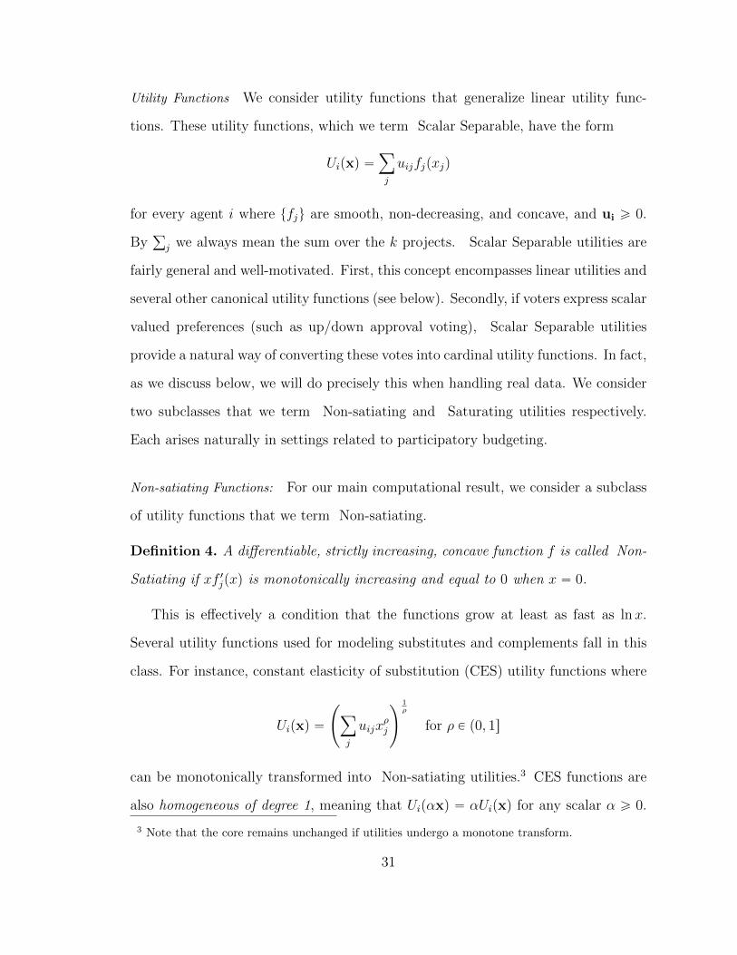
Utility Functions We consider utility functions that generalize linear utility func-
tions. These utility functions, which we term Scalar Separable, have the form
Uipxq “ÿ
j
uijfjpxjq
for every agent i where tfju are smooth, non-decreasing, and concave, and ui ě 0.
Byř
j we always mean the sum over the k projects. Scalar Separable utilities are
fairly general and well-motivated. First, this concept encompasses linear utilities and
several other canonical utility functions (see below). Secondly, if voters express scalar
valued preferences (such as up/down approval voting), Scalar Separable utilities
provide a natural way of converting these votes into cardinal utility functions. In fact,
as we discuss below, we will do precisely this when handling real data. We consider
two subclasses that we term Non-satiating and Saturating utilities respectively.
Each arises naturally in settings related to participatory budgeting.
Non-satiating Functions: For our main computational result, we consider a subclass
of utility functions that we term Non-satiating.
Definition 4. A differentiable, strictly increasing, concave function f is called Non-
Satiating if xf 1jpxq is monotonically increasing and equal to 0 when x “ 0.
This is effectively a condition that the functions grow at least as fast as lnx.
Several utility functions used for modeling substitutes and complements fall in this
class. For instance, constant elasticity of substitution (CES) utility functions where
Uipxq “
˜
ÿ
j
uijxρj
¸1ρ
for ρ P p0, 1s
can be monotonically transformed into Non-satiating utilities.3 CES functions are
also homogeneous of degree 1, meaning that Uipαxq “ αUipxq for any scalar α ě 0.
3 Note that the core remains unchanged if utilities undergo a monotone transform.
31

When ρ “ 1, this captures linear utilities. When ρ Ñ 0, these are Cobb-Douglas
utilities which for αij ą 0 such thatř
j αij “ 1, can be written as Uipxq “ś
j xαijj .
Saturating Functions: Note that Scalar Separable utilities assume goods are divisible.
Fractional allocations make sense in their own right in several scenarios: Budget
allocations between goals such as defense and education at a state or national level
are typically fractional, and so are allocations to improve utilities such as libraries,
parks, gyms, roads, etc. However, in the settings for which we have real data, the
projects are indivisible and have a monetary cost sj, so that we have the additional
constraint xj P t0, sju on the allocations. We therefore need utility functions that
model budgets in individual projects. These utility functions must also be simple to
account for the limited information elicited in practice. For example, in the voting
data that we use in our experiments, each voter receives an upper bound on how
many projects she can select, and the ballot cast by a voter is simply the subset
of projects she selects. A related voting scheme implemented in practice, called
Knapsack Voting [81], has similar elicitation properties. For modeling these two
considerations, we consider Saturating utilities.
Definition 5. Saturating utility functions Uipxq have the formř
j uij min´
xjsj, 1¯
.
For converting our voting data into a Saturating utility, we set sj to be the budget
of project j, and set uij to 1 if agent i votes for project j and 0 otherwise. Note that
if xj “ sj, then the utility of any agent who voted for this item is 1. This implies the
total utility of an agent is the number (or total fraction) of items that he voted for
that are present in the final allocation. Clearly, Saturating utilities do not satisfy
Definition 4. However, in a full paper we connect Non-satiating and Saturating
utilities by developing an approximation algorithm and heuristic for computing core
allocations in the saturating model using results developed for the Non-satiating
32

model [63].
2.4.1 Computing the Lindahl Equilibrium
In a fairly general public goods setting, there is a market based notion of fairness
due to Lindahl [118] and Samuelson [148] termed the Lindahl equilibrium, which is
based on setting different prices for the public goods for different agents. The market
on which the Lindahl equilibrium is defined is a mixed market of public and private
goods. We present a definition below that is specialized to just a public goods market
relevant for participatory budgeting.
Definition 6. In a public goods market with budget B, per-voter prices p1,p2, ...,pn
each in Rk` and allocation x P Rk
` constitute a Lindahl equilibrium if the following
two conditions hold:
1. For every agent i, the utility Uipyiq is maximized subject to pi ¨yi ď Bn when
yi “ x; and
2. The profit defined as př
i piq ¨ z ´ z1, subject to z ě 0 is maximized when
z “ x.
The price vector for every agent is traditionally interpreted as a tax. However,
unlike in private goods markets, in our case these prices (or taxes) are purely hy-
pothetical; we are only interested in the allocation that results at equilibrium (in
fact, we eliminate the prices from our characterization of the equilibrium). Under
innocuous conditions for the mixed public and private goods market, Foley proved
that the Lindahl equilibrium exists and lies in the core [71]. This remains true in our
specialized instance of the problem; the omitted proof is a trivial adaption from [71].
Thus, computing a Lindahl equilibrium is sufficient for the purpose of computing a
core allocation. However, Foley only proves existence of the equilibrium via a fixed
point argument that does not lend itself to efficient computation.
33

Our first result is a characterization of the Lindahl equilibrium that uses the
optimality conditions to eliminate the price variables entirely.
Theorem 3. An allocation x ě 0 corresponds to a Lindahl equilibrium if and only
if
ÿ
i
ˆ
uijf1jpxjq
ř
m uimxmf1mpxmq
˙
ďn
B(2.2)
for all items j, where this inequality is tight when xj ą 0.
Proof. We prove the statement for more general utility functions, tUipxqu. Recall
the definition of Lindahl equilibrium from Definition 6: Condition (1) implies that
there is a dual variable λi for every agent such that
@jB
BxjUipxq ď λipij (2.3)
with the inequality being tight if xj ą 0. Condition (1) in Definition 6 also implies
thatř
j pijxj “ Bn for all i. Multiplying Equation (2.3) by xj, noting that the
inequality is tight when xj ą 0, and summing,
@i,ÿ
j
xjB
BxjUipxq “
ÿ
j
λipijxj “ λipBnq
Rearranging
@i, λi “n
B
ÿ
j
xjB
BxjUipxq (2.4)
Similarly, Condition (2) in Definition 6 implies that @xj,ř
i pij ď 1 where the
inequality is tight when xj ą 0. Substituting into Inequality (2.3) and summing, we
have:
@xj,ÿ
i
B
BxjUipxq
λiď 1 (2.5)
34

with the inequality being tight when xj ą 0. Using Equation (2.4) to eliminate λi in
Inequality (2.5), we finally obtain
@xj,ÿ
i
B
BxjUipxq
ř
m xmB
BxmUipxq
ďn
B
with the inequality being tight when xj ą 0. Taking the appropriate partial deriva-
tives in the scalar separable utility model yields the theorem statement.
We now present our main computational result that builds on the characterization
above to give the first non-trivial polynomial time method for computing the Lindahl
equilibrium. We need the non-satiation assumption on the functions tfju given in
Definition 4.
Theorem 4. When Uipxq “ř
j uijfjpxjq where tfju satisfy Definition 4, the Lindahl
equilibrium (and therefore a core solution) is the solution to a convex program.
Proof. Recall the characterization of the Lindahl equilibrium from Theorem 3. Define
zj “ xjf1jpxjq. Note that xj “ 0 iff zj “ 0. Since fj satisfies non-satiation, this
function is continuous and monotonically increasing, and hence invertible. Let hj be
this inverse such that hjpzjq “ xj. Let rjpzjq “ hjpzjqzj “ 1f 1jpxjq. The Lindahl
equilibrium characterization therefore simplifies to:
ÿ
i
ˆ
uijř
m uimzm
˙
ďn
Brjpzjq
with the inequality being tight when zj ą 0. Let Rjpzjq be the indefinite integral of
rj (with respect to zj). Define the following potential function
Φpzq “ÿ
i
log
˜
ÿ
j
uijzj
¸
´
´ n
B
¯
ÿ
j
Rjpzjq (2.6)
35

We claim that Φpzq is concave in z. The first term in the summation is trivially
concave. Also, since f 1jpxjq is a decreasing function, 1f 1jpxjq is increasing in xj.
Since rjpzjq “ 1f 1jpxjq, this is increasing in xj and hence in zj. This implies Rjpzjq
is convex, showing the second term in the summation is concave as well. It is easy to
check that the optimality conditions of maximizing Φpzq subject to z ě 0 are exactly
the conditions for the Lindahl equilibrium. This shows that the Lindahl equilibrium
corresponds to the solution to the convex program maximizing Φpzq.
It is not difficult to argue that an approximately optimal solution to the convex
program gives an approximate core solution, which implies polynomial time compu-
tation to arbitrary accuracy. We note that the non-satiation condition essentially
implies that fjpxjq should grow faster than lnxj. In combination with the assump-
tion that fjpxjq is concave, this leaves us with a broad class of concave functions for
which the Lindahl equilibrium and hence the core can be efficiently computed. Fur-
thermore, it is easy to see that for linear utility functions, maximizing the potential
in equation 2.6 reduces to the proportional fairness program.
2.5 Conclusion and Open Directions
In this chapter, we addressed the problem of allocating divisible public resources
according to budget constraints. We adapted a stability notion from game theory
called the core as a novel solution concept for group fairness in the allocation of
public goods. We demonstrated that for linear utilities, the celebrated proportional
fairness program computes a core solution. Furthermore, for linear utilities, we were
able to adapt techniques from differential privacy to give an approximately truthful
mechanism for computing an approximate core solution. For more general utilities,
we turned to the Lindahl equilibrium for existence, and we initiated the computa-
tional study of the Lindahl equilibrium. We expressed the equilibrium (and hence
36

the core) purely in terms of common allocation variables. In a sense, this is a mirror
image of the role common prices play in private good markets. Having common
allocations instead of prices poses some challenges in computation and mechanism
design, but has the advantage that we can compute equilibria for a wider class of
utility functions.
Our work is just the first step towards understanding these equilibria. We do
not yet understand the computational complexity for more general utility functions.
Are they as hard as general concave games? Our truthfulness result uses a scoring
function based on the gradient; it would be nice to generalize this result to other
utility functions, as well as design simpler, more practical schemes.
37

3
Fair Indivisible Decisions
In this chapter, we continue examining the core as a fair solution concept for public
goods. However, we no longer assume that we can allocate fractional goods. Instead,
we assume that we must integrally choose a set of goods to allocate. Our compu-
tational results vary based on the constraints imposed on such a solution set. Our
algorithms are quite distinct from those for divisible goods. We provide constant ad-
ditive approximation algorithms for matroid and matching constraints that operate
by local search, and then give a rounding algorithm for packing constraints. Matroid
constraints allow us to model voting, in particular, multi-winner elections and mul-
tiple referendums. Packing constraints allow us to model participatory budgeting
when projects must be completely funded or completely rejected.
Acknowledgements. These results are published in [66], which is joint work with
Kamesh Munagala and Nisarg Shah. Conversations with Rupert Freeman, Vincent
Connitzer, and Paul Golz were also very helpful.
38
3.1 Introduction
Consider an example to highlight what an indivisible public decision problem might
look like, and why fairness might be a concern. Suppose that the next time you
vote, you see that there are four referendums for your consideration on the ballot,
all of which concern the allocation of various public goods in your city: A = a new
school, B = enlarging the public library, C = renovating the community college,
and D = improving a museum. In 2016, residents of Durham, North Carolina faced
precisely these options [122]. Suppose the government has resources to fund only two
of the four projects, and the (hypothetical) results were as follows: a little more than
half of the population voted for pA,Bq, a little less than half voted for pC,Dq, and
every other combination received a small number of votes. Which projects should
be funded?
If we naıvely tally the votes, we would fund A and B, and ignore the preferences of
a very large minority. In contrast, funding A and C seems like a reasonable compro-
mise. Of course, it is impossible to satisfy all voters, but given a wide enough range
of possible outcomes, perhaps we can find one that fairly reflects the preferences of
large subsets of the population. This idea is not captured by fairness axioms like
proportionality or their approximations [53], which view fairness from the perspec-
tives of individual agents. Indeed, in the aforementioned example, every allocation
gives zero utility to some agent, and would be deemed equally good according to
such fairness criteria.
In this chapter, we consider a fairly broad model for public goods allocation that
generalizes much of the prior work in the literature [53, 63, 16, 70, 41, 136]. There
is a set of voters (or agents) N “ rns. Public goods are modeled as elements of a
ground set W . We denote m “ |W |. An outcome c is a subset of W . Let F Ď 2W
denote the set of feasible outcomes.
39

The utility of agent i for element j P W is denoted uij P Rě0. We assume that
agents have additive utilities, i.e., the utility of agent i under outcome c P F is
uipcq “ř
jPc uij. Since we are interested in scale-invariant guarantees, we assume
without loss of generality that maxjPW uij “ 1 for each agent i, so that uij P r0, 1s for
all i, j. Crucially, this does not restrict the utility of an agent for an outcome to be 1:
uipcq can be as large as m. Specifically, let Vi “ maxcPF uipcq, and Vmax “ maxiPN Vi.
Our results differ by the feasibility constraints imposed on the outcome. We consider
three types of constraints, special cases of which have been studied previously in
literature.
Matroid Constraints. In this setting, we are given a matroid M over the ground set
W , and the feasibility constraint is that the chosen elements must form a basis of
M (see [112] for a formal introduction to matroids).
This generalizes the public decision making setting introduced by [53]. In this
setting, there is a set of issues T , and each issue t P T has an associated set of
alternatives At “ tat1, . . . , atktu, exactly one of which must be chosen. Agent i has
utility utipatjq if alternative atj is chosen for issue t, and utilities are additive across
issues. An outcome c chooses one alternative for every issue. It is easy to see that if
the ground set is YtAt, the feasibility constraints correspond to a partition matroid.
We note that public decision making in turn generalizes the classical setting of private
goods allocation [119, 41, 136] in which private goods must be divided among agents
with additive utilities, with each good allocated to exactly one agent.
Matroid constraints also capture multi-winner elections in the voting literature
(see, e.g. [16]), in which voters have additive utilities over candidates, and a commit-
tee of at most k candidates must be chosen. This is captured by a uniform matroid
over the set of candidates.
40

Matching Constraints. In this setting, the elements are edges of an undirected graph
GpV,Eq, and the feasibility constraint is that the subset of edges chosen must form a
matching. Matchings constraints in a bipartite graph can be seen as the intersection
of two matroid constraints. Matching constraints are a special case of the more
general packing constraints we consider below.
Packing Constraints. In this setting, we impose a set of packing constraints Ax ď b,
where xj P t0, 1u is the indicator denoting whether element j is chosen in the outcome.
Suppose A is a Kˆm matrix, so that there are K packing constraints. By scaling, we
can assume akj P r0, 1s for all k, j. Note that even for one agent, packing constraints
encode independent set. Thus, to make the problem tractable, we assume b is
sufficiently large, in particular, bk “ ω plogKq for all k P t1, 2, . . . , Ku. This is in
contrast to matroid and matching constraints, for which single-agent problems are
polynomial time solvable. A classic measure of how easy it is to satisfy the packing
constraints is the width ρ [138]:
ρ “ maxkPrKs
ř
jPrms akj
bk. (3.1)
Packing constraints capture the general Knapsack setting, in which there is a
set of m items, each item j has an associated size sj, and a set of items of total size
at most B must be selected. This setting is motivated by participatory budgeting
applications [1, 81, 80, 63, 75, 70, 25], in which the items are public projects, and
the sizes represents the costs of the projects. Knapsack uses a single packing
constraint. Multiple packing constraints can arise if the projects consume several
types of resources, and there is a budget constraint for each resource type. For
example, consider a statewide participatory budgeting scenario where each county
has a budget than can only be spent on projects affecting that county, the state has
some budget that can be spent in any county, and projects might affect multiple
41
counties. In such settings, it is natural to assume a small width, i.e., that the budget
for each resource is such that a large fraction (but not all) of the projects can be
funded. We note that the aforementioned multi-winner election problem is a special
case of the Knapsack problem with unit sizes.
3.1.1 Fairness Properties
As with divisible goods, we define fairness desiderata for indivisible public goods by
generalizing appropriate desiderata from the private goods setting such as Pareto
optimality, which is a weak notion of efficiency, and proportionality, which is a per-
agent fair share guarantee. For convenience, we define these concepts explicitly for
outcomes consisting of indivisible goods.
Definition 7. An outcome c satisfies Pareto optimality if there is no other outcome
c1 such that uipc1q ě uipcq for all agents i P N , and at least one inequality is strict.
Recall that Vi is the maximum possible utility agent i can derive from a feasible
outcome.
Definition 8. The proportional share of an agent i P N is Propi :“ Vin
. For β P
p0, 1s, we say that an outcome c satisfies β-proportionality if uipcq ě β ¨ Propi for
all agents i P N . If β “ 1, we simply say that c satisfies proportionality.
The difficulty in this setting stems from requiring integral outcomes, and not al-
lowing randomization. In the absence of randomization, it is reasonably straightfor-
ward to show that we cannot guarantee β-proportionality for any β P p0, 1s. Consider
a problem instance with two agents and two feasible outcomes, where each outcome
gives a positive utility to a unique agent. In any feasible outcome, one agent has
zero utility, which violates β-proportionality for every β ą 0.
To address this issue, [53] introduced the novel relaxation of proportionality up to
one issue in their public decision making framework, inspired by a similar relaxation
42
called envy-freeness up to one good in the private goods setting [119, 41]. They
say that an outcome c of a public decision making problem satisfies proportionality
up to one issue if for all agents i P N , there exists an outcome c1 that differs from
c only on a single issue and uipc1q ě Propi. Proportionality up to one issue is a
reasonable fairness guarantees only when the number of issues is larger than the
number of agents; otherwise, it is vacuous and is satisfied by all outcomes. Thus, it
is perfectly reasonable for some applications (e.g., three friends choosing a movie list
to watch together over the course of a year), but not for others (e.g., when thousands
of residents choose a handful of public projects to finance). In fact, it may produce
an outcome that may be construed as unfair if it does not reflect the wishes of large
groups of voters. Thus, in this chapter we address the following question posed
by [53]:
Is there a stronger fairness notion than proportionality in the public de-
cision making framework...? Although such a notion would not be sat-
isfiable by deterministic mechanisms, it may be satisfied by randomized
mechanisms, or it could have novel relaxations that may be of independent
interest.
Our primary contributions are twofold. First, we define a fairness notion for pub-
lic goods allocation that is stronger than proportionality, ensures fair representation
of groups of agents, and in particular, provides a meaningful fairness guarantee even
when there are fewer goods than agents. Second, we provide polynomial time al-
gorithms for computing integer allocations that approximately satisfy this fairness
guarantee for a variety of settings generalizing the public decision making framework
and participatory budgeting. Our fairness notion is an adaptation of the core. Be-
low, we define the notion of notion of a core outcome for indivisible goods. Note that
we study the core defined on proportional shares of utility rather than proportional
43

shares of endowments.
Definition 9. Given an outcome c, we say that a set of agents S Ď N form a
blocking coalition if there exists an outcome c1 such that p|S|nq ¨ uipc1q ě uipcq for
all i P S and at least one inequality is strict. We say that an outcome c is a core
outcome if it admits no blocking coalitions.
Again, note that non-existence of blocking coalitions of size 1 is equivalent to
proportionality, and non-existence of blocking coalitions of size n is equivalent to
Pareto optimality. Hence, a core outcome is both proportional and Pareto optimal.
However, the core satisfies a stronger property of being, in a sense, Pareto optimal
for coalitions of any size, provided we scale utilities based on the size of the coalition.
Another way of thinking about the core is to view it as a fairness property that
enforces a proportionality-like guarantee for coalitions: e.g., if half of all agents have
identical preferences, they should be able to get at least half of their maximum
possible utility. It is important to note that the core provides a guarantee for every
possible coalition. Hence, in satisfying the guarantee for a coalition S, a solution
cannot simply make a single member i P S happy and ignore the rest as this would
likely violate the guarantee for the coalition Sztiu.
Unfortunately, since a proportional outcome is not guaranteed to exist (even
allowing for multiplicative approximations), the same is true for the core. However,
an additive approximation to the core still provides a meaningful guarantee, even
when there are fewer elements than agents because it provides a non-trivial guarantee
to large coalitions of like-minded agents.
Definition 10. For δ, α ě 0, an outcome c is a pδ, αq-core outcome if there exists
no set of agents S Ď N and outcome c1 such that
|S|
n¨ uipc
1q ě p1` δq ¨ uipcq ` α
44

for all i P S, and at least one inequality is strict.
A p0, 0q-core outcome is simply a core outcome. A pδ, 0q-core outcome satisfies δ-
proportionality. Similarly, a p0, 1q-core outcome c satisfies the following relaxation of
proportionality that is slightly weaker than proportionality up to one issue: for every
agent i P N , uipcq ` 1 ě Propi. We note that this definition, and by extension, our
algorithms satisfy scale invariance, i.e., they are invariant to scaling the utilities of
any individual agent. Because we normalize utilities of the agents, the true additive
guarantee is α times the maximum utility an agent can derive from a single element.
Since an outcome can have many elements, an approximation with small α remains
meaningful.
The advantage of an approximate core outcome is that it fairly reflects the will of
a like-minded subpopulation relative to its size. An outcome satisfying approximate
proportionality only looks at what individual agents prefer, and may or may not
respect the collective preferences of sub-populations. We present such an instance
in Example 1 (Section 3.2.1), in effect showing that an approximate core outcome is
arguably more fair.
In our results, we will assume δ ă 1 to be a small constant, and focus on making α
as small as possible. In particular, we desire guarantees on α that exhibit sub-linear
or no dependence on n, m, or any other parameters. Deriving such bounds is the
main technical focus of our work.
3.1.2 Results
We present algorithms to find approximate core outcomes under matroid, matching,
and general packing constraints. Our first result (Section 3.3) is the following:
Theorem 5. If feasible outcomes are constrained to be bases of a matroid, then a
p0, 2q-core outcome is guaranteed to exist, and for any ε ą 0, a p0, 2`εq-core outcome
can be computed in time polynomial in n,m, and 1ε.
45
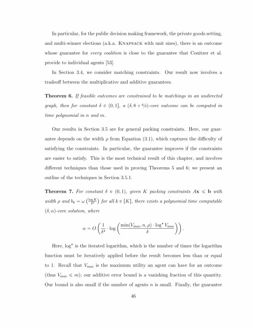
In particular, for the public decision making framework, the private goods setting,
and multi-winner elections (a.k.a. Knapsack with unit sizes), there is an outcome
whose guarantee for every coalition is close to the guarantee that Conitzer et al.
provide to individual agents [53].
In Section 3.4, we consider matching constraints. Our result now involves a
tradeoff between the multiplicative and additive guarantees.
Theorem 6. If feasible outcomes are constrained to be matchings in an undirected
graph, then for constant δ P p0, 1s, a pδ, 8` 6δq-core outcome can be computed in
time polynomial in n and m.
Our results in Section 3.5 are for general packing constraints. Here, our guar-
antee depends on the width ρ from Equation (3.1), which captures the difficulty of
satisfying the constraints. In particular, the guarantee improves if the constraints
are easier to satisfy. This is the most technical result of this chapter, and involves
different techniques than those used in proving Theorems 5 and 6; we present an
outline of the techniques in Section 3.5.1.
Theorem 7. For constant δ P p0, 1q, given K packing constraints Ax ď b with
width ρ and bk “ ω`
logKδ2
˘
for all k P rKs, there exists a polynomial time computable
pδ, αq-core solution, where
α “ O
ˆ
1
δ4¨ log
ˆ
minpVmax, n, ρq ¨ log˚ Vmax
δ
˙˙
.
Here, log˚ is the iterated logarithm, which is the number of times the logarithm
function must be iteratively applied before the result becomes less than or equal
to 1. Recall that Vmax is the maximum utility an agent can have for an outcome
(thus Vmax ď m); our additive error bound is a vanishing fraction of this quantity.
Our bound is also small if the number of agents n is small. Finally, the guarantee
46

improves for small ρ, i.e., as the packing constraints become easier to satisfy. For
instance, in participatory budgeting, if the total cost of all projects is only a constant
times more than the budget, then our additive guarantee is close to a constant.
Note that Vmax (which is bounded by m), n, and ρ are all unrelated quantities —
either could be large with the other two being small. In fact, in Section 3.5, we state
the bound more generally in terms of what we call the maximally proportionally fair
value R, which informally captures the (existential) difficulty of finding a proportion-
ally fair allocation. The quantity minpVmax, n, ρq stems from three different bounds
on the value of R.
Also, note that the lower bound on b in the above theorem is necessary: if
b “ Op1q, then no non-trivial approximation to the core can be guaranteed, even
when ρ is a constant. To see this, consider a complete bipartite graph GpL,R,Eq,
where |L| “ |R| “ m2. The vertices are the elements of the ground set W , and
the constraints ensure that feasible outcomes are independent sets, which can be
encoded with constraints of the form Ax ď b where b “ 1 (and the width is ρ “ 2).
There are two agents. Agent 1 has unit utility for each vertex in L, and zero utility
for each vertex in R, while agent 2 has unit utility for each vertex in R. A feasible
outcome is forced to choose either vertices from L or vertices from R, and hence gives
zero utility to at least one agent. But this agent can deviate and choose an outcome
with utility m2, which is then scaled down to m4. Hence, no feasible outcome is
pδ,m4q-core for any δ ą 0.
3.1.3 Related Work
A simpler property than the core is proportionality, which like the core, is impossible
to satisfy to any multiplicative approximation using integral allocations. To address
this problem, [53] defined proportionality up to one issue in the public decision
making framework, inspired by related notions for private goods. This guarantee is
47

satisfied by the integral outcome maximizing the Nash welfare objective, which is the
geometric mean of the utilities to the agents. For public goods, this objective is not
only NP-Hard to approximate to any multiplicative factor, but approximations to
the objective also do not retain the individual fairness guarantees.
We extend the notion of additive approximate proportionality to additive ap-
proximate core outcomes, which provides meaningful guarantees even when there
are fewer goods than agents. Unlike proportionality, we show in Section 3.2.1 that
the approach of computing the optimal integral solution to the Nash welfare objective
fails to provide a reasonable approximation to the core. Therefore, for our results
about matroid constraints (Theorem 5) and matching constraints (Theorem 6), we
slightly modify the integer Nash welfare objective and add a suitable constant term
to the utility of each agent. We show that maximizing this smooth objective function
achieves a good approximation to the core. However, maximizing this objective is
still NP-hard [70], so we devise local search procedures that run in polynomial time
and still give good approximations of the core. In effect, we make a novel connection
between appropriate local optima of smooth Nash Welfare objectives and the core.
Fairness on Endowments. Classically, the core is defined in terms of agent endow-
ments, not scaled utilities. This is the notion we explored in Chapter 2. The notion
of core with endowments logically implies a number of fairness notions considered
in multi-winner election literature, such as justified representation, extended jus-
tified representation [16], and proportional justified representation [149]. Approval-
based multi-winner elections are a special case of packing constraints, in which voters
(agents) have binary utilities over a pool of candidates (elements), and we must se-
lect a set of at most B candidates. The idea behind proportional representation is
to define a notion of large cohesive groups of agents with similar preferences, and
ensure that such coalitions are proportionally represented. The core on endowments
48

represents a more general condition that holds for all coalitions of agents, not just
those that are large and cohesive. Nevertheless, our local search algorithms for The-
orems 5 and 6 are similar to local search algorithms for proportional approval voting
(PAV) [156, 17] that achieve proportional representation. It would be interesting to
explore the connection between these various notions in greater depth.
Strategyproofness. In this work, we will not consider game-theoretic incentives for
manipulation for two reasons. First, even for the restricted case of private goods
allocation, preventing manipulation leads to severely restricted mechanisms. For
instance, [152] shows that the only strategyproof and Pareto efficient mechanisms are
dictatorial, and thus highly unfair, even when there are only two agents with additive
utilities over divisible goods. Second, our work is motivated by public goods settings
with a large number of agents, such as participatory budgeting, wherein individual
agents often have limited influence over the final outcome. It would be interesting
to establish this formally, using notions like strategyproofness in the large [14].
3.2 Prelude: Nash Social Welfare
Our approach to computing approximate core solutions revolves around the Nash
social welfare, which is the product (or equivalently, the sum of logarithms) of agent
utilities. This objective is commonly considered to be a natural tradeoff between
the fairness-blind utilitarian social welfare objective (maximizing the sum of agent
utilities) and the efficiency-blind egalitarian social welfare objective (maximizing the
minimum agent utility). This function also has the advantage of being scale invariant
with respect to the utility function of each agent, and in general, preferring more
equal distributions of utility.
49

3.2.1 Integer Nash Welfare and Smooth Variants
The integer Max Nash Welfare (MNW) solution [41, 53] is an outcome c that maxi-
mizesř
iPN lnuipcq. More technically, if every integer allocation gives zero utility to
at least one agent, the MNW solution first chooses a largest set S of agents that can
be given non-zero utility simultaneously, and maximizes the product of utilities to
agents in S.
[53] argue that this allocation is reasonable by showing that it satisfies propor-
tionality up to one issue for public decision making. A natural question is whether
it also provides an approximation of the core. We answer this question in the nega-
tive. The example below shows that even for public decision making (a special case
of matroid constraints), the integer MNW solution may fail to return a pδ, αq-core
outcome, for any δ “ opmq and α “ opmq.
Example 1. Consider an instance of public decision making [53] with m issues and
two alternatives per issue. Specifically, each issue t has two alternatives tat1, at2u, and
exactly one of them needs to be chosen. There are two sets of agents X “ t1, . . . ,mu
and Y “ tm` 1, . . . , 2mu. Every agent i P X has uiipai1q “ 1, and utility 0 for all
other alternatives. Every agent i P Y has utipat2q “ 1 and utipa
t1q “ 1m for all issues
i P t1, 2, . . . ,mu. Visually, this is represented as follows.
a11 a12 a21 a22 . . . am1 am2u1PX 1 0 0 0 . . . 0 0u2PX 0 0 1 0 . . . 0 0
......
......
......
...umPX 0 0 0 0 . . . 1 0uiPY 1m 1 1m 1 . . . 1m 1
The integer MNW outcome is c “ pa11, a21, . . . , a
m1 q because any other outcome
gives zero utility to at least one agent. However, coalition Y can deviate, choose
outcome c1 “ pa12, a22, . . . , a
m2 q, and achieve utility m for each agent in Y . For c to be
50
a pδ, αq-core outcome, we need
Di P Y : p1` δq ¨ uipcq ` α ě|Y |
|Y | ` |X|¨ uipc
1q ñ 1` δ ` α ě
m
2.
Hence, c is not a pδ, αq-core outcome for any δ “ opmq and α “ opmq. In contrast,
it is not hard to see that c1 is a p0, 1q-core outcome because each agent in X gets
utility at most one in any outcome.
Further, note that outcome c gives every agent utility 1. Since Propi ď 1 for each
agent i, c satisfies proportionality, and yet fails to provide a reasonable approximation
to the core. One may argue that c1, which is a p0, 1q-core outcome, is indeed fairer
because it respects the utility-maximizing choice of half of the population; the other
half of the population cannot agree on what they want, so respecting their top
choice is arguably a less fair outcome. Hence, the example also shows that outcomes
satisfying proportionality (or proportionality up to one issue) can be very different
from and less fair than approximate core outcomes.
Smooth Nash Welfare. One issue with the Nash welfare objective is that it is sensitive
to agents receiving zero utility. We therefore consider the following smooth Nash
welfare objective:
F pcq :“ÿ
iPN
ln p`` uipcqq (3.2)
where ` ě 0 is a parameter. Note that ` “ 0 coincides with the Nash welfare
objective. The case of ` “ 1 was considered by [70], who showed it is NP-Hard to
optimize. Recall that we normalized agent utilities so that each agent has a maximum
utility of 1 for any element, so when we add ` to the utility of agent i, it is equivalent
to adding `maxj uij to the utility of agent i when utilities are not normalized.
We show that local search procedures for the smooth Nash welfare objective, for
appropriate choices of `, yield a p0, 2q-core outcome for matroid constraints (Sec-
tion 3.3) and a`
δ, O`
1δ
˘˘
-core outcome for matching constraints (Section 3.4). In
51

contrast, we present Example 2 to show that optimizing any fixed smooth Nash wel-
fare objective cannot guarantee a good approximation to the core, even with a single
packing constraint, motivating the need for a different algorithm.
3.2.2 Fractional Max Nash Welfare Solution
For general packing constraints, we use a fractional relaxation of the Nash welfare
program. A fractional outcome consists of a vector w such that wj P r0, 1s measures
the fraction of element j chosen. The utility of agent i under this outcome is uipwq “řmj“1wjuij.
The fractional Max Nash Welfare (MNW) solution is a fractional allocation that
maximizes the Nash welfare objective (without any smoothing). Define the packing
polytope as:
P “!
w P r0, 1sm |řmj“1 akjwj ď bk, @k P rKs
)
Then the fractional MNW solution is arg maxcPPř
i lnuipcq.
It is easy to show that the fractional MNW allocation lies in the core using the
same rough proof idea as in the previous chapter. Unfortunately, for the allocation
of public goods, it can be shown that the fractional MNW outcome can be irrational
despite rational inputs [3], preventing an exact algorithm. For our approximation
results, a fractional solution that approximately preserves the utility to each agent
would suffice, and we prove the following theorem in Appendix 8.2.
Theorem 8. For any ε, δ ą 0, we can compute a fractional pδ, εq-core outcome in
time polynomial in the input size and log 1εδ
.
3.3 Matroid Constraints
We now consider public goods allocation with matroid constraints. In particular,
we show that when the feasibility constraints encode independent sets of a matroid
52

M, maximizing the smooth Nash welfare objective in Equation (3.2) with ` “ 1
yields a p0, 2q-core outcome. However, optimizing this objective is known to be NP-
hard [70]. We also show that given ε ą 0, a local search procedure for this objective
function (given below) yields a p0, 2 ` εq-core outcome in polynomial time, which
proves Theorem 5.
Algorithm. Fix ε ą 0. Let γ “ ε4m
, where m “ |W | is the number of elements.
Recall that there are n agents.
1. Start with an arbitrary basis c of M.
2. Compute F pcq “ř
iPN lnp1` uipcqq.
3. Let a swap be a pair pj, j1q such that j P c, j1 R c, and c1 “ cztju Y tj1u is also
a basis of M.
4. Find a swap such that F pc1q ´ F pcq ě nγm
.
• If such a swap exists, then perform the swap, i.e., update c Ð c1, and go
to Step (2).
• If no such swap exists, then output c as the final outcome.
Analysis. First, we show that the local search algorithm runs in time polynomial
in n, m, and 1ε. Note that F pcq “ Opn lnmq because in our normalization, each
agent can have utility at most m. Thus, the number of iterations is O pm2 logmεq.
Finally, each iteration can be implemented in Opn ¨ m2q time by iterating over all
pairs and computing the change in the smooth Nash welfare objective.
Next, let c˚ denote the outcome maximizing the smooth Nash welfare objective
with ` “ 1, and pc denote the outcome returned by the local search algorithm. We
show that c˚ is a p0, 2q-core outcome, while pc is a p0, 2` εq-core outcome.
53
For outcome c, define Fipcq “ lnp1` uipcqq. Fix an arbitrary outcome c. For an
agent i with uipcq ą 0, we have that for every element j P c:
Fipcq ´ Fipcztjuq ďuij
uipcq ` 1´ uijď
uijuipcq
.
This holds because lnpx` hq ´ lnx ď hx
for x ą 0 and h ě 0. Summing this over all
j P c gives
ÿ
jPc
Fipcq ´ Fipcztjuq ďÿ
jPc
uijuipcq
“uipcq
uipcq“ 1.
For an agent i with uipcq “ 0, we trivially haveř
jPc Fipcq´Fipcztjuq “ 0. Summing
over all agents, we have that for every outcome c:
ÿ
jPc
F pcq ´ F pcztjuq “ÿ
iPN
ÿ
jPc
Fipcq ´ Fipcztjuq ď n. (3.3)
We now use the following result:
Lemma 2 ([112]). For every pair of bases c and c1 of a matroid M, there is a
bijection f : c Ñ c1 such that for every j P c, cztju Y tfpjqu is also a basis.
Using the above lemma, combined with the fact that lnpx ` hq ´ lnx ě hx`h
for
x ą 0 and h ě 0, we have that for all c, c1:ÿ
jPc
F pcztju Y tfpjquq ´ F pcztjuq ěÿ
i
ÿ
jPc
uifpjquipcq ` 1´ uij ` uifpjq
ěÿ
iPS
ÿ
j1Pc1
uij1
uipcq ` 2“ÿ
iPS
uipc1q
uipcq ` 2. (3.4)
We now provide almost similar proofs for the approximations achieved by the
global optimum c˚ and the local optimum pc.
Global optimum. Suppose for contradiction that c˚ is not a p0, 2q-core outcome.
Then, there exist a subset S of agents and an outcome c1 such that for all i P S,
|S|
n¨ uipc
1q ě uipc
˚q ` 2,
54

and at least one inequality is strict. Rearranging the terms and summing over all
i P S, we obtain:
ÿ
iPS
uipc1q
uipc˚q ` 2ąÿ
iPS
n
|S|“ n.
Combining this with Equation (3.4), and subtracting Equation (3.3) yields:
ÿ
jPc˚
pF pc˚ztju Y tfpjquq ´ F pc˚qq ą 0.
This implies existence of a pair pj, fpjqq such that F pc˚ztju Y tfpjquq ´ F pc˚q ą 0,
which contradicts the optimality of c˚ because c˚ztju Y tfpjqu is also a basis of M.
Local optimum. Similarly, suppose for contradiction that pc is not a p0, 2` εq-core
outcome. Then, there exist a subset S of agents and an outcome c1 such that for all
i P S,
|S|
n¨ uipc
1q ě uippcq ` 2` ε ą p1` γq puippcq ` 2q .
Here, the final transition holds because γ ă εpm ` 2q ď εpuippcq ` 2q. Again,
rearranging and summing over all i P S, we obtain:
ÿ
iPS
uipc1q
uippcq ` 2ą p1` γq
ÿ
iPS
n
|S|ě n ¨ p1` γq.
Once again, combining this with Equation (3.4), and subtracting Equation (3.3)
yields:ÿ
jPpc
pF ppcztju Y tfpjquq ´ F ppcqq ą nγ.
This implies existence of a pair pj, fpjqq such that F ppcztjuYtfpjquq´F ppcq ą nγm,
which violates local optimality of pc because pcztju Y tfpjqu is also a basis of M.
55

Lower Bound. While a p0, 2q-core always outcome exists, we show in the following
example that a p0, 1´ εq-core outcome is not guaranteed to exist for any ε ą 0.
Lemma 3. For ε ą 0 and matroid constraints, p0, 1 ´ εq-core outcomes are not
guaranteed to exist.
Proof. Consider the following instance of public decision making where we have
several issues and must choose a single alternative for each issue, a special case of
matroid constraints. There are n agents, where n is even. There are m “ pn´2q`n2
issues. The first n ´ 2 issues correspond to unit-value private goods, i.e., each such
issue has n alternatives, and each alternative gives utility 1 to a unique agent and
utility 0 to others. The remaining n2 issues are “pair issues”; each such issue has`
n2
˘
alternatives, one corresponding to every pair of agents that gives both agents in
the pair utility 1 and all other agents utility 0.
It is easy to see that every integer allocation gives utility at most 1 to at least two
agents. Consider the deviating coalition consisting of these two agents. They can
choose the alternative that gives them each utility 1 on every pair issue, and split
the n´ 2 private goods equally. Thus, they each get utility n2` pn´ 2q2 “ n´ 1.
For the outcome to be a p0, αq-core outcome, we need 1 ` α ě p2nq ¨ pn ´ 1q. As
n Ñ 8, this requires α Ñ 1. Hence, for any ε ą 0, a p0, 1 ´ εq-core outcome is not
guaranteed to exist.
Note that Theorem 5 shows existence of a p0, 2q-core outcome, which is there-
fore tight up to a unit additive relaxation. Whether a p0, 1q-core outcome always
exists under matroid constraints remains an important open question. Interestingly,
we show that such an outcome always exists for the special case of private goods
allocation, and, in fact, can be achieved by maximizing the smooth Nash welfare
objective.
56
Lemma 4. For private goods allocation, maximizing the smooth Nash welfare objec-
tive with ` “ 1 returns a p0, 1q-core outcome.
Proof. There is a set of agents N and a set of private goods M . Each agent i P N
has a utility function ui : 2M Ñ Rě0. Utilities are additive, so uipSq “ř
gPS uiptguq
for all S Ď M . For simplicity, we denote uig fi uiptguq. Without loss of generality,
we normalize the utility of each agent such that maxgPM uig “ 1 for each i. An
allocation A is a partition of the set of goods among the agents; let Ai denote the
bundle of goods received by agent i. We want to show that an allocation maximizing
the objectiveś
iPNp1` uipAiqq is a p0, 1q-core outcome.
Let A denote an allocation maximizing the smooth Nash welfare objective with
` “ 1. We assume without loss of generality that every good is positively valued by
at least one agent. Hence, ujpAjq “ 0 must imply Aj “ H.
For agents i, j P N with Aj ‰ H (hence ujpAjq ą 0), and good g P Aj, moving g
to Ai should not increase the objective function. Hence, for each g P Aj, we have
`
1` uipAi Y tguq˘
¨`
1` ujpAjz tguq˘
ď`
1` uipAiq˘
¨`
1` ujpAjq˘
.
Using additivity of utilities, this simplifies to
uig1` uipAiq
ďujg
1` ujpAjq ´ ujgď
ujgujpAjq
. (3.5)
For every agent j P N with Aj ‰ H and good g P Aj, define pg “ ujgujpAjq.
Abusing the notation a little, for a set T Ď M define pT “ř
gPT pg. Then, from
Equation (3.5), we have that for all players i P N and goods g PM ,
p1` uipAiqq ¨ pg ě uig. (3.6)
Suppose for contradiction that A is not a p0, 1q-core outcome. Then, there exists
a set of agents S Ď N and an allocation B of the set of all goods to agents in S such
57
that p|S|nq ¨ uipBiq ě 1` uipAiq for every agent i P S, and at least one inequality is
strict. Rearranging the terms and summing over i P S, we have
ÿ
iPS
uipBiq
1` uipAiqąÿ
iPS
n
|S|“ n. (3.7)
We now derive a contradiction. For agent i P S, summing Equation (3.6) over
g P Bi, we get
p1` uipAiqq ¨ pBi ě uipBiq ñuipBiq
1` uipAiqď pBi .
Summing this over i P S, we get
ÿ
iPS
uipBiq
1` uipAiqďÿ
iPS
pBi “ÿ
gPM
pg “ÿ
jPN s.t.Aj‰H
ÿ
gPAj
ujgujpAjq
“ÿ
jPN s.t.Aj‰H
ujpAjq
ujpAjqď n.
However, this contradicts Equation (3.7).
3.4 Matching Constraints
We now present the algorithm proving Theorem 6. We show that if the elements
are edges of an undirected graph GpV,Eq, and the feasibility constraints encode a
matching, then for constant δ P p0, 1s, a pδ, 8` 6δq-core always exists and is efficiently
computable. The idea is to again run a local search on the smooth Nash welfare
objective in Equation (3.2), but this time with ` « 1` 4δ.
Algorithm. Recall that there are n agents. Let |V | “ r and |E| “ m. Let κ “ 2δ.
For simplicity, assume κ P N. Our algorithm is inspired by the PRAM algorithm for
approximate maximum weight matchings due to [92], and we follow their terminology.
Given a matching c, an augmentation with respect to c is a matching T Ď Ezc. The
size of the augmentation is |T |. Let MpT q denote the subset of edges of c that have
58

a vertex which is matched under T . Then, the matching pczMpT qq Y T is called the
augmentation of c using T .
1. Start with an arbitrary matching c of G.
2. Compute F pcq “ř
i ln p1` 2κ` uipcqq.
3. Let C be the set of all augmentations with respect to c of size at most κ.
• If there exists T P C such that F ppczMpT qq Y T q ´ F pcq ě nκr
, perform
this augmentation (i.e., let c Ð pczMpT qq Y T ) and go to Step (2).
• Otherwise, output c as the final outcome.
Analysis. The outline of the analysis is similar to the analysis for matroid con-
straints. First, we show that the algorithm runs in polynomial time. Again, recall
that each agent has utility at most m. Thus, F pcq “ Opn ¨ lnmq. Because each im-
provement increases the objective value by at least npκrq, the number of iterations
is Opκr lnmq “ Opm2δq. Each iteration can be implemented by naıvely going over
all Opmκq subsets of edges of size at most κ, checking if they are valid augmentations
with respect to c, and whether they improve the objective function by more than
npκrq. The local search therefore runs in polynomial time for constant δ ą 0.
Let c denote the outcome returned by the algorithm. We next show that c is
indeed a pδ, 8 ` 3κq-core outcome. Suppose for contradiction that this is not true.
Then, there exist a subset of agents S and a matching c1 such that for all i P S,
|S|
n¨ uipc
1q ě p1` δq ¨ uipcq ` 8` 3κ ě p1` δq ¨ puipcq ` 3κ` 1q ,
and at least one inequality is strict (the last inequality is because δ P p0, 1s). Rear-
ranging and summing over all i P S, we obtain
ÿ
iPS
uipc1q
uipcq ` 3κ` 1ą p1` δq ¨
ÿ
iPS
n
|S|“ n ¨ p1` δq. (3.8)
59

For j P E, define wj “ř
iPNuij
uipcq`1and w1j “
ř
iPNuij
uipcq`3κ`1. Let W “
ř
jPcwj,
and W 1 “ř
jPc1 w1j. It is easy to check that
W ď n and W 1ě n ¨ p1` δq, (3.9)
where the latter follows from Equation (3.8). Further note that wj ě w1j for all j.
For an augmentation T with respect to c, define gainpT q “ř
jPT w1j´
ř
jPMpT qwj.
The next lemma is a simple generalization of the analysis in [92]; we give the adap-
tation here for completeness.
Lemma 5. Assuming weights wj ě w1j for all edges j, for any integer κ ě 1 and
matchings c and c1, there exists a multiset OPT of augmentations with respect to c
such that:
• For each T P OPT , T Ď c1 and |T | ď κ;
• |OPT | ď κr; and
•ř
TPOPT gainpT q ě κ ¨W 1 ´ pκ` 1q ¨W .
Proof. We follow [92] in the construction the multiset OPT of augmentations with
respect to c out of edges in c1. Let c4c1 be the symmetric difference of matchings c
and c1 consisting of alternating paths and cycles. For every cycle or path d P c4c1,
let Td be be set of edges d X c1. For all Td with |Td| ď κ, just add TS to OPT κ
times (note that OPT is a multiset, not a set). For Td with |Td| ą κ, we break up
Td into multiple smaller augmentations. To do so, index the edges in Td from 1 to
|Td| and add |Td| different augmentations to OPT by considering starting at every
index in Td and including the next κ edges in Td with wrap-around from |Td| to 1.
Now we must argue that OPT as we have constructed it satisfies the conditions
of the lemma. The first point, that @T P OPT, T Ď c1 and |T | ď κ, follows trivially
60

from the construction. The second point also follows easily from observing that we
add κ augmentations to OPT for every d P cX c1, and graph G has r vertices.
To see the third point, note that every edge in c1zc is contained in at least κ
augmentations in OPT . On the other hand, for every edge e P czc1, there are no
more than κ` 1 augmentations T P OPT such that e PMpT q (recall MpT q are the
edges of c with a vertex matched under T ). This can happen, for example, if TS
happens to be a path of length κ ` 1. Finally, for the edges j P c1 X c, the weight
w1j ď wj. Putting these facts together, the third point of the lemma follows.
Consider the set of augmentations OPT from Lemma 5. For T P OPT ,
F ppczMpT qq Y T q ´ F pcq
“
´
F ppczMpT qq Y T q ´ F pczMpT qq¯
´
´
F pcq ´ F pczMpT qq¯
ěÿ
iPN
˜
ř
TPS uijuipcq ` 2κ` 1`
ř
jPT uij´
ř
jPMpT q uij
uipcq ` 2κ` 1´ř
jPMpT q uij
¸
ěÿ
iPN
˜
ř
jPT uij
uipcq ` 3κ` 1´
ř
jPMpT q uij
uipcq ` 1
¸
“ÿ
jPT
w1j ´ÿ
jPMpT q
wj “ gainpT q.
Here, the second transition holds because hpx` hq ď lnpx` hq ´ lnx ď hx for all
x ě 1 and h ě 0, and the third transition holds due to |T | ď κ and |MpT q| ď 2|T | ď
2κ. Therefore, we have:ÿ
TPOPT
F ppczMpT qq Y T q ´ F pcq ěÿ
TPOPT
gainpT q ě κ ¨W 1´ pκ` 1q ¨W
ě κ ¨ n ¨ p1` δq ´ pκ` 1q ¨ n “ n,
where the second transition follows from Lemma 5, and the third transition follows
from Equation (3.9). Since |OPT | ď κr, there exists an augmentation T P OPT
61

with F ppczMpT qq Y T q ´ F pcq ě nκr, which violates local optimality of c. This
completes the proof of Theorem 6.
Lower Bound. We give a stronger lower bound for matchings than the lower bound
for matroids in Lemma 3.
Lemma 6. A pδ, αq-core outcome is not guaranteed to exist for matching constraints,
for any δ ě 0 and α ă 1.
Proof. This example shows that Consider the graph K2,2 (the complete bipartite
graph with two vertices on each side). This graph has four edges, and two disjoint
perfect matchings.
Let there be two agents. Agent 1 has unit utility for the edges of one matching,
while agent 2 has unit utility for the edges of the other matching. Any integer
outcome gives zero utility to one of these agents. This agent can deviate and obtain
utility 2. Hence, for an outcome to be a pδ, αq-core outcome, we need p1`δq ¨0`α ě
p12q ¨ 2, which is impossible for any δ ě 0 and α ă 1.
3.5 General Packing Constraints
In this section, we study approximation to the core under general packing constraints
of the form Ax ď b. Recall that there are m elements, Vi is the maximum possible
utility that agent i can receive from a feasible outcome, and Vmax “ maxiPN Vi.
We prove a statement slightly more general than Theorem 7. We first need the
following concept. Given an instance of public goods allocation subject to packing
constraints, we define the notions of an r-proportionally fair (r-PF) outcome, a
maximally proportionally fair (MPF) outcome, and the MPF value of the instance.
Definition 11 (MPF Outcome). For r ą 0, we say that a fractional outcome w is
62

r-proportionally fair (r-PF) if it satisfies:
uipwq ěVir´ 1, @i P N.
The maximally proportionally fair (MPF) value R of an instance is the least value r
such that there exists an r-PF outcome. For simplicity, we say that an R-PF outcome
is a maximally proportionally fair (MPF) outcome.
This concept is crucial to stating and deriving our approximation results. In
words, an r-PF outcome gives each agent an r fraction of its maximum possible
utility Vi (which can be thought of as the fair share guarantee of the agent), if the
agent is given 1 unit of utility for free. Thus, a smaller value of r indicates a better
solution. The MPF value R denotes the best possible guarantee. The additive 1 in
Def. 11 can be replaced by any positive constant; we choose 1 for simplicity.
We now show an upper bound for R that holds for all instances. Recall from
Equation (3.1) that ρ is the width of the instance.
Lemma 7. R ď minpVmax, n, ρq, and an MPF outcome is computable in polynomial
time.
Proof. To show that R is well-defined, note that for r “ Vmax, an r-PF outcome w
simply requires uipwq ě 0, which is trivially achieved by every outcome. Therefore,
R is well-defined, and R ď Vmax. Next, R ď n follows from the fact that there
exist fractional outcomes satisfying proportionality (e.g., the outcome w obtained
by taking the uniform convex combination of the n outcomes that give optimal to
each individual agent). Finally, to show R ď ρ, consider the outcome w in which
wj “1ρ
for each element j. Clearly, uipwq ěViρ
for all i. Further, Aw ď b is satisfied
trivially due to the fact that ρ is the width of the packing constraints.
To compute the value of R as well as an MPF outcome, we first note that the
value of Vi for each agent i can be computed by solving a separate LP. Then, we
63

consider the following LP:
Maximize r (3.10)
ř
jPW uijwj ě Vi ¨ r ´ 1 @i P rns
Aw ď bwj P r0, 1s @j P W
Here, Aw ď b are the packing constraints of the instance, and r is a variable rep-
resenting 1r. Thus, maximizing r minimizes r, which yields an MPF outcome.
This can be accomplished by solving n ` 1 linear programs, which can be done in
polynomial time.
Our main result in this section uses any r-PF outcome, and provides a guarantee
in terms of log r. Thus, we do not need to necessarily compute an exact MPF
outcome. We note that an MPF outcome can be very different from a core outcome.
Yet, an MPF outcome gives each agent a large fraction of its maximum possible
utility, subject to a small additive relaxation. As we show below, this helps us find
integral outcomes that provide good approximations of the core.
3.5.1 Result and Proof Idea
Our main result for this section (Theorem 7) can be stated more precisely. Recall that
log˚ is the iterated logarithm, which is the number of times the logarithm function
must be iteratively applied before the result becomes less than or equal to 1.
Theorem 9. Fix constant δ P p0, 1q. Suppose we are given a set of K packing
constraints Ax ď b such that bk “ ω`
logKδ2
˘
for all k P rKs. Let R be the MPF value
of this instance. Then there exists a polynomial time computable pδ, αq-core outcome,
where
α “ O
ˆ
1
δ4¨ log
ˆ
R ¨ log˚ Vmax
δ
˙˙
.
64
We first note that the above result cannot be obtained by maximizing the smooth
Nash welfare objective; we present Example 2, which demonstrates this using only
one packing constraint. To be precise, the example shows that no single value of
parameter ` in the smooth Nash welfare objective can provide a polylog additive
guarantee for all instances. While it may be possible to choose the value of ` based
on the instance, it does not seem trivial.
Example 2. Recall that in the Knapsack setting, we are given a set of elements of
different sizes, and our goal is to select a subset of elements with total size at most
a given budget B. We show that for any ` ą 0, there exists a Knapsack instance
in which maximizing the smooth Nash welfare objective F pcq “ř
iPN ln p`` uipcqq
returns an outcome that is not a pOpm12´εq, Opm34´εqq-core outcome. This is in
contrast to Theorem 9, which provides a pδ, αq-core guarantee where δ is constant
and α is logarithmic in the number of elements.
Fix ` ą 0. Set a large budget B ě `4. There are m “ B14`B elements, of which
B14 are large elements of size B34 and the remaining B are small elements of unit
size. There are n ě 4B14 logp2Bq agents. Each agent has unit utility for each large
element. A subset of αn agents are special (we determine α later). These special
agents have unit utility for each small element, while the remaining agents have zero
utility for the small elements.
The idea is to show that when α is sufficiently small, the smooth Nash welfare
objective will choose only the large elements. However, α can still be large enough
so that the special agents can deviate, and get a large amount of utility.
Note that maximizing the smooth Nash welfare objective returns a Pareto efficient
solution, and hence can be one of two types: it either chooses all large elements (which
gives utility B14 to each agent), or it chooses B14´r large elements and rB34 small
elements. For the former to have a larger smooth Nash welfare objective value, we
65

need that for each 1 ď r ď B14,
lnpB14` `q ą α ln
`
rB34` pB14
´ rq ` `˘
` p1´ αq lnpB14´ r ` `q.
This holds true if
ln
ˆ
B14 ` `
B14 ` `´ r
˙
ą α ln`
rB34` pB14
´ rq ` `˘
.
Since 0 ă ` ď B14, the above is true for each 1 ď r ď B14 if
ln
ˆ
2B14
2B14 ´ 1
˙
ą α ln`
B14B34`B14
˘
.
This is true when
ln
ˆ
1`1
2B14
˙
ě α lnp2Bq.
Since lnp1` xq ě x2 for x P r0, 1s, the above holds when:
α ď1
4B14 lnp2Bq.
Let us set α “ 14B14 lnp2Bq
. Choosing all large elements maximizes the smooth Nash
welfare objective. Since n ě 1α, there is at least one special agent. The special
agents get utility B14 each. If they deviate and choose all the small elements, they
get (scaled down) utility
αB “B
4B14 lnp2Bq“
B34
4 lnp2Bq.
Hence, for the solution to be a pδ, αq-core outcome, we need p1 ` δq ¨ B14 `
α ě B34p4 lnp2Bqq. Since m “ ΘpBq, this shows that the outcome is not a
pOpm12´εq, Opm34´εqq-core outcome for any constant ε ą 0, as required.
66

We take a different approach. Our idea is to start with a fractional core solution
x. Suppose it assigns utility U˚i to agent i. Fix δ ą 0, and consider the following
program.
Minimize α (3.11)
α ` p1` δq ¨ř
jPW uijwj ě U˚i @i P rns
Aw ď bwj P t0, 1u @j P Wα ě 0
For the optimum value α˚, we obtain an outcome that is pδ, α1q-core for every
α1 ą α. To see this, take a subset of agents S and a feasible utility vector U1 under
any other (even fractional) outcome. Because x is a core outcome, there exists i P S
such that U˚i ě p|S|nq ¨ U1i . For α1 ą α, the ILP solution implies
α1 ` p1` δq ¨ÿ
jPW
uijwj ą U˚i ě|S|
n¨ U 1i ,
which implies that the solution is pδ, α1q-core according to Definition 10.
However, α˚ obtained from this program can be rather large, as illustrated in
the following example. Consider the Knapsack setting with m unit-size projects.
There is an overall budget B “ m2. For every feasible integral outcome c, let there
be an agent with utility 1 for every project in c and 0 for all other projects. Thus,
there are`
mm2
˘
agents. The fractional core outcome gives weight 12 to each project,
thus giving utility Vi2 “ m4 to each agent i. However, every integral outcome
gives utility 0 to at least one agent, which implies α˚ “ Ωpmq.
This example shows that when there are a large number of agents, we cannot
achieve Theorem 9 by hoping to approximately preserve the utilities to all agents
with respect the fractional core solution. However, note that in the above example,
though there is one agent who gets very little utility, this agent has no incentive to
67

deviate if she is given one unit of utility for free. This insight leads us to our analysis
below, which is based on rounding the fractional core solution x.
Let us apply randomized rounding to x. Instead of using Chernoff bounds to
ensure that there are no “violations” (i.e., that no agent receives utility that is too
far from its utility under the core outcome x), we hope to bound the expected number
of such violations. If there are few such agents, we still have an approximate core
outcome because if this small coalition of agents deviates, its utility under a new
outcome will be scaled down by a large factor. Unfortunately, it can be shown that
bounding the expected number of deviations by a sufficiently small number forces
α “ Ωplog Vmaxq. This is better than α “ Ωpmq from our previous approach, but still
much larger than the bound we want to achieve in Theorem 9 when the width ρ is
small.
This brings up the main technical idea. We observe that an MPF outcome,
though not in the core, provides a reasonably large utility to each agent. We add
a small amount of this outcome to the fractional core before applying randomized
rounding. We are now ready to present our algorithm.
3.5.2 Algorithm
Fix δ P p0, 1q, and let γ “ δ8.
1. Compute the (approximate) fractional core solution x as in Theorem 8, where
xj is the fraction of element j chosen.
2. Let y be an MPF outcome as in Definition 11.
3. Let z “ p1´ γqx` γy.
4. For each j P W , choose j to be in the outcome c independently with probability
zj “ p1´ γqzj.
68
3.5.3 Analysis
We show that this algorithm yields, with at least a constant probability, a feasible
outcome that satisfies the guarantee in Theorem 9. This directly shows the existence
of such an outcome. Note that the fractional Max Nash Welfare solution x can be
irrational, but we can compute an approximation in polynomial time (see Theorem 8
for details), which does not change our guarantee asymptotically. Further, y can be
computed in polynomial time (Lemma 7). Hence, the algorithm runs in expected
polynomial time.
We first show that the packing constraints are satisfied. Since we scale down z
by a factor p1 ´ γq before rounding, we have Az ď p1 ´ γqb. Since b “ ω`
logKδ2
˘
, a
simple application of Chernoff bounds shows that with probability at least 0.99, the
rounded solution c satisfies Ac ď b. Therefore, if we show that the algorithm also
yields the desired approximation of the core with at least a constant probability (16
to be precise), we will be done by applying union bound to the two events, feasibility
and good approximation to the core.
For the ease of presentation, we suppress constants throughout the proof and use
asymptotic notation liberally. We also assume that Vmax “ ωp1q since otherwise there
is a trivial p0, Op1qq-core outcome that chooses a null outcome, giving zero utility to
each agent.
Grouping Agents. In order to analyze our algorithm, we partition the agents into
groups with exponentially decreasing values of Vi. Recall that Vi is the maximum
utility that agent i can get from any outcome. Set Q0 “ log Vmax, and for ` “
0, 1, . . . , L´ 1, define group G` as:
G` “ ti P N | Q` ě log Vi ě Q``1u .
Here, for ` “ 0, 1, . . . , L´ 1, we define: Q``1 “ 2 logQ`.
69

We callG0, . . . , GL´1 the heavy groups. We choose L so thatQL “ Θ´
log R log˚ Vmax
γ3
¯
.
This implies L “ Ωplog˚ Vmaxq “ ωp1q, since Vmax “ ωp1q. For agent i in a heavy
group, Vi ě eQL ě 2RLγ3ą 2R. Thus, the utility that the MPF solution provides to
agent i is at least ViR´ 1 ě Vi
2R.
Finally, we put the remaining agents (with a small Vi) in a light group defined as
follows:
GL “ ti P N | log Vi ď QLu .
The MPF solution may not provide any guarantee for the utility of agents in this
group.
Bounding Violations of Utility Preservation. We want to bound the number of agents
whose utilities are far from those under the core outcome. First, we need a specialized
Chernoff bound.
Lemma 8. Let X1, X2, . . . , Xq be independent random variables in r0, 1s, and let
X “řqj“1Xj. For γ P p0, 12q, suppose ErXs “ p1 ´ γq ¨ A ` γ ¨ B for A,B ě 0.
Then
PrrX ă p1´ 2γq ¨ As ď e´γ3
2maxpB,A2q
Proof. We first state the standard theorem for Chernoff bounds. Let X1, X2, . . . , Xq
be independent random variables in r0, 1s, and let X “řqj“1Xj. For any ε P p0, 1q,
we have:
Pr rX ă p1´ εqErXss ď e´ε2
2ErXs
Equivalently, for any η ă ErXs,
Pr rX ă ErXs ´ ηs ď e´η2
2ErXs
70

Lemma 8 follows from considering two cases. First, suppose p1´ γqA ě B.
PrrX ă p1´ γq2As ď PrrX ă p1´ γqErXss ď e´γ2
2ErXs
ď e´γ2
2maxpγB,p1´γqAq
ď e´γ3
2maxpB,Aq
In the other case, if p1´ γqA ă B, then γB ď ErXs ď p1` γqB. Then
PrrX ă p1´ γqAs ď PrrX ď ErXs ´ γBs
ď e´γ2 B2
2ErXs ď e´γ2 B2
2p1`γqB
ď e´γ3
2Bď e´
γ3
2p1´γqA
ď e´γ3
4A
Recall that x is the fractional MNW solution, y is the fractional MPF solution,
and our algorithm applies randomized rounding to their scaled down mixture p1 ´
γqz “ p1 ´ γq2x ` γp1 ´ γqy. Let pUi denote the utility of agent i under the final
integral outcome obtained by randomly rounding p1 ´ γqz. Recall that U˚i is the
utility of agent i under the core outcome x. We want to show that pUi is either
multiplicatively or additively close to U˚i for most agents. For a heavy group G`,
where ` P t0, 1, . . . , L´ 1u, define
F` “!
i P G`
ˇ
ˇ
ˇ
pUi ă p1´ 3γqU˚i
)
.
Simiarly, for the light group GL, define
FL “
"
i P GL
ˇ
ˇ
ˇ
ˇ
pUi ă min
ˆ
p1´ 3γqU˚i , U˚i ´
4QL
γ4
˙*
.
We will use Lemma 8 to bound the sizes of F` for ` P t0, 1, . . . , Lu as follows.
Theorem 10. We have that:
71

1. With probability at least 23, we have |F`| ď1
2LeQ`¨|G`|, @` P t0, 1, . . . , L´ 1u.
2. With probability at least 12, we have |FL| ď1
2eQL¨ |GL|.
Thus, with probability at least 16, both the above inequalities hold simultaneously.
Proof. We prove the first and the second part of Theorem 10 separately by consider-
ing the heavy groups and the light group in turn. The combined result follows from
the union bound.
Case 1: Heavy Groups Consider a heavy group G` for 0 ď ` ă L. Recall that the
MPF solution provides utility at least Vip2Rq to each agent in a heavy group. Hence,
we have:
E”
pUip1´ γqı
“ uipzq ě p1´ γq ¨ U˚i ` γ ¨
Vi2R
. (3.12)
The key point is that even if U˚i is small, the expected utility is at least a term
that is proportional to Vi. This will strengthen our application of Chernoff bounds.
Using Lemma 8 with A “ U˚i and B “ Vip2Rq, we have:
Pr”
pUi ă p1´ 3γq ¨ U˚i
ı
ď Pr
«
pUi1´ γ
ă p1´ 2γq ¨ U˚i
ff
ď e´γ3
4
Vi2R ď e´
γ3
8RQ2`
ď e´Q`¨logL ď e´pQ``2 logL`log 6q ď1
6L2eQ`, (3.13)
where the second inequality holds because log Vi ě 2 logQ`, the third holds because
Q` “ Ω´
RLγ3
¯
, and the fourth holds because L “ ωp1q.
We are now ready to prove the first part of Theorem 10. Let η` “1
6L2eQ`. Recall
that F` consists of agents in G` for which pUi ă p1 ´ 3γq ¨ U˚i . Using the linearity of
expectation in Equation (3.13), we have ErF`s ď η` ¨ |G`|. By Markov’s inequality,
72

Pr r|F`| ą 3L ¨ η` ¨ |G`|s ď13L. Applying the union bound over the L heavy groups,
we have that with probability at least 23,
|F`| ď 3L ¨ η` ¨ |G`| “1
2LeQ`¨ |G`|, @` P t0, 1, . . . , L´ 1u,
which proves the first part of Theorem 10.
Case 2: Light Group For the light group, note that log Vi ď QL. For this group, the
MPF solution may not provide any non-trivial guarantee on the utility to the agents.
Since the expected utility can now be small, we have to allow additive approximation
as well. Recall that FL consists of agents in GL for whom pUi ă p1´ 3γq ¨ U˚i as well
as pUi ă U˚i ´ 4QLγ4. We again consider two cases.
Case 1. If U˚i ď4γ4QL, then pUi ě U˚i ´
4QLγ4
trivially.
Case 2. Otherwise, U˚i ě4QLγ4
, and using Lemma 8, we have:
Pr”
pUi ă p1´ 3γqU˚i
ı
ď Pr
«
pUi1´ γ
ă p1´ 2γqU˚i
ff
ď e´γ3
4U˚i ď e
´γ3
4¨4QLγ4 ď
1
4eQL.
It is easy to check that the final transition holds because γ ă 1 is a constant and
QL “ ωp1q.
Note that none of the agents in FL are in Case 1. Hence, by Markov’s inequality,
we again have:
Pr
„
|FL| ě1
2eQL¨ |GL|
ď1
2,
which proves the second part of Theorem 10.
Approximate Core. We showed that with probability at least 16, our algorithm
returns a solution that satisfies conditions in both parts of Theorem 10. We now
73

show that such a solution is the desired approximate core solution. The main idea is
that when a set of agents deviate, the fraction of agents in a group G` that are in F`
is small enough such that even if they receive their maximum possible utility, which
is eQ` , their scaled down utility is at most a constant.
Theorem 11. For every coalition S and every possible outcome h, there exists an
agent i P S s.t.
|S|
n¨ uiphq ď p1` 8γq ¨ pUi `
5QL
γ4.
Proof. Let W “ Nz YL`“0 F`. In other words, W is the set of agents who either
receive a good multiplicative approximation to their expected utility in the core
(for the heavy groups), or a good additive approximation to their expected utility
in the core (for the light group). In particular, for every i P W , we have pUi ě
min´
p1´ 3γq ¨ U˚i , U˚i ´
4QLγ4
¯
, which implies
U˚i ď1
1´ 3γ¨ pUi `
4QL
γ4. (3.14)
Consider a set of agents S that may want to deviate, and let h be any (even
fractional) outcome. There are two cases:
Case 1. Suppose |SXW | ě p1´γq ¨ |S|. Then, due to the fractional core optimality
condition (see Section 3.2.2), we have:
ÿ
iPSXW
Uiphq
U˚iď n.
Note that in polynomial time, Theorem 8 only finds an approximate solution whose
utilities tUiu withř
iPSXWUiphq
Uiď np1 ` ηq for small η ą 0. It is easy to check this
does not alter the rest of the proof and adds a small multiplicative factor of p1` ηq
74

to the final approximation bound. We ignore this factor for simplicity and simply
assume tU˚i u are the optimal MNW utilities. The above implies |S|n¨ř
iPSXWuiphq
U˚iď
|S| ď 11´γ
¨ |S XW |.
Therefore, there exists an agent i P S XW such that
|S|
n¨ uiphq ď
1
1´ γ¨ U˚i ď
1
1´ γ¨
ˆ
1
1´ 3γ¨ pUi `
4QL
γ4
˙
,
where the last transition is due to Equation (3.14) and the fact that i P W . Finally, it
is easy to check that for γ “ δ8 ď 18, we have 1p1´γq¨p1´3γq
ď 1`8γ and 4p1´γq ď 5,
which yields:
|S|
n¨ uiphq ď p1` 8γq ¨ pUi `
5QL
γ4. (3.15)
Case 2. Otherwise, |SzW | ě γ|S|. In this case, we want to show that there exists an
agent i P SzW such that p|S|nq ¨ uiphq ď 1γ. Because pUi ě 0 and QL “ ωp1q, such
an agent will also satisfy Equation (3.15). We show this by taking two sub-cases.
First, suppose the light group satisfies |SXFL| ěγ2|S|. Then: |S| ď 2
γ¨ |SXFL| ď
2γ¨ |FL|. Thus, for any agent i P FL, we have
|S|
n¨ uiphq ď
2
γn¨ |FL| ¨ Vi ď
2
γn¨|GL|
2eQL¨ Vi ď
1
γ.
Here, the second transition follows from Theorem 10. To see why the third transition
holds, note that |GL| ď n, and that log Vi ď QL because i P GL.
Similarly, in the other sub-case, suppose |S X FL| ďγ2|S|. Then, there exists a
heavy group ` P t0, 1, . . . , L ´ 1u such that |S X F`| ěγ2L|S|. This means |S| ď
2Lγ¨ |S X F`| ď
2L㨠|F`|.
Again, for an arbitrary agent i P F`, we have:
|S|
n¨ uiphq ď
2L
γn¨ |F`| ¨ Vi ď
2L
γn¨|G`|
2LeQ`¨ Vi ď
1
γ.
75
Once again, the third transition follows from Theorem 10, and the fourth transition
holds because |G`| ď n and log Vi ď Q` as i P G`. Putting everything together, the
theorem follows.
Since γ “ δ8
and QL “ Θ´
log R log˚ Vmaxγ
¯
, Theorem 11 implies |S|n¨ uiphq ď
p1 ` δq ¨ pUi ` α˚, where α˚ “ O´
1δ4¨ log
´
R¨log˚ Vmax
δ
¯¯
. The existence of such an
agent implies that a solution satisfying Theorem 10 is a pδ, αq-core solution for every
α ą α˚, which completes the proof of Theorem 9.
3.6 Conclusion and Open Directions
We considered the problem of fairly allocating public goods. We argued that the core,
which is a generalization of proportionality and Pareto efficiency, and approximations
of the core provide reasonable fairness guarantees in this context. Given that no
integral outcome may be in the core, we presented efficient algorithms to produce
integral outcomes that are constant or near-constant approximations of the core,
thereby also establishing the non-trivial existence of such outcomes. Note that our
algorithms for matroid and matching constraints that globally optimize the smooth
Nash welfare objective achieve exact rather than approximate Pareto efficiency, in
addition to an approximation of the core. An interesting question is whether the
same guarantee can be provided (regardless of computation time) for general packing
constraints.
Another natural question following our work is to tighten our upper bounds, or to
establish matching lower bounds. For instance, we show the existence of a p0, 2q-core
outcome for matroid constraints (Theorem 5), but our lower bound only shows that
a p0, 1 ´ εq-core outcome may not exist. This leaves open the question of whether
a p0, 1q-core outcome always exists. Existence of p0, 1q-core outcome is also an open
question for matching constraints. For packing constraints, it is unknown if even a
76
pδ, αq-core outcome exists for constant δ ą 0 and α “ Op1q. This also remains an
open question for the endowment-based notion of core.
At a higher level, we established connections between approximating the core in
our multi-agent environment and the problem of finding the optimal (i.e., utility-
maximizing) outcome for a single agent. For instance, given matching constraints,
our algorithm uses the idea of short augmenting paths from fast PRAM algorithms.
This hints at the possibility of a deeper connection between efficiency results and
existence results.
77
4
Fair Clustering
In this chapter, we consider a very different kind of problem in public decision making:
centroid clustering. One can think of the task of clustering a group of data points as
a public resource allocation problem where the data points are the agents and the
possible centers are the public goods. Now we think of the agents as having unit
demand utilities (or costs, more precisely), in the sense that they only care about their
favorite center, in the sense of the center that is closest to them in some metric (this
is a standard model for facility location problems, for example). We will continue
with this basic approach of modeling the costs of public decisions in metric spaces
in the subsequent chapters. We adapt our notion of core as a fairness guarantee for
clustering so that we ensure that we do not ignore large cohesive groups of agents
for the sake of a global objective. Due to the different model of valuations, we term
our fairness notion proportionality instead of core in this context, but it is in fact an
application of the core under a particular utility model. Note that this is a different
notion of proportionality than is employed for resource allocation problems. Our
work introduces this form of proportionality as a novel solution concept in clustering
and systematically studies its computation.
78
Acknowledgements. These results are from joint work with Xingyu Chen, Charles
Lyu, and Kamesh Munagala, and is under review at the 36th International Confer-
ence on Machine Learning (ICML) at the time of this writing [45].
4.1 Introduction
The data points in machine learning are often real human beings. There is legit-
imate concern that traditional machine learning algorithms that are blind to this
fact may inadvertently exacerbate problems of bias and injustice in society [102].
Motivated by concerns ranging from the granting of bail in the legal system to the
quality of recommender systems, researchers have devoted considerable effort to de-
veloping fair algorithms for the canonical supervised learning tasks of classification
and regression [61, 107, 87, 106, 161, 56, 137, 162, 105, 83, 91].
We extend this work to a canonical problem in unsupervised learning: centroid
clustering. In centroid clustering, we want to partition data into k clusters by
choosing k “centers” and then matching points to one of the centers. This is a
classic context for clustering work [84, 43, 13], and is perhaps best known as the
setting for the celebrated k-means heuristic (independently discovered many times,
see [94] for a brief history). We provide a novel group based notion of fairness as
proportionality, inspired by recent related work on the fair allocation of public re-
sources [16, 53, 66, 74]. We suppose that data points represent the individuals to
whom we wish to be fair, and that these agents prefer to be clustered accurately
(that is, they prefer their cluster center to be representative of their features). A
solution is fair if it respects the entitlements of groups of agents, where we assume
that a subset of agents is entitled to choose a center for themselves if they constitute
a sufficiently large fraction of the population with respect to the total number of
clusters (e.g., 1k of the population, if we are clustering into k groups). The guaran-
tee must hold for all subsets of sufficient size, and therefore does not hinge on any
79
particular a priori knowledge about which points should be protected. This is in line
with other recent observations that information about which individuals should be
protected may not be available in practice [91].
Consider an example of the problem of proportional clustering. We want to assign
incoming college students to one of k themed communities. Each student fills out
a survey providing information about their preferred community, e.g., quiet hours,
community activities, etc. We choose the k themes in light of this information,
and we want to do so in a way that is fair to the incoming students. The idea is
that any 1k fraction of the incoming students should be allowed to form their own
community if they prefer. A proportional solution is one for which there is no such
large group that prefers to choose their own theme over the theme or themes to which
we assigned them. In that sense, one can also see proportionality as a no justified
complaint guarantee, a stability condition, and a fairness condition.
For an example in a different context, consider medical data. Each data point
may represent an individual, and clustering is a basic data analysis tool that can
influence further research and development. One approach to fairness is to ensure
that the clustering obscures protected demographic information by ensuring that all
clusters have comparable ratios of all relevant demographics [47]. While this makes
sense when clustering is used to generate features for downstream decision making
like loan applications, it is less clearly appropriate in an application like medicine,
where protected information like sex, race, and age may all be highly medically
relevant. Instead, we are inspired by the idea of precision medicine [52], to tailor
research, development, and treatment to account for variability in the base popula-
tion. Toward that end, proportional clustering guarantees that the data analyst will
not inadvertently ignore large groups of data while clustering for the sake of some
global objective. It does this in a robust fashion that does not require the a priori
definition of specific protected groups.
80
4.1.1 Preliminaries and Definition of Proportionality
We have a set N of |N | “ n individuals or data points, and a set M of |M| “ m
feasible cluster centers. We will sometimes consider the important special case where
M “ N (i.e., where one is only given a single set of points as input), but most of our
results are for the general case where we make no assumption about M X N . For
all i, j P N YM, we have a distance dpi, jq satisfying the triangle inequality. Our
task is centroid clustering as treated in the classic k-median, k-means, and k-center
problems. We wish to open a set X ĎM of |X| “ k centers (assume |M| ě k), and
then match all points in N to their closest center in X. For a particular solution
X and agent i P N , let DipXq “ minxPX dpi, xq. In general, a good clustering
solution X will have small values of DipXq, although the aforementioned objectives
differ slightly in how they measure this. In particular, the k-median objective isř
iPN DipXq, the k-means objective isř
iPN pDipXqq2, and the k-center objective is
maxiPN DipXq.1
To define proportional clustering, we assume that individuals prefer to be closer to
their center in terms of distance (i.e., ensuring that the center is more representative
of the point). Any subset of at least rrnks individuals is entitled to choose r centers.
We call a solution proportional if there does not exist any such sufficiently large set
of individuals who, using the number of centers to which they are entitled, could
produce a clustering among themselves that is to their mutual benefit in the sense
of Pareto dominance. More formally, a blocking coalition is a set S Ď N of at least
rrnks points and a set Y Ď M of at most r centers such that DipY q ă DipXq for
all i P S. It is easy to see that because DipXq “ minxPX dpi, xq, this is functionally
equivalent to Definition 12; a larger blocking coalition necessarily implies a blocking
1 We note that this is very similar to the related facility location problem, although in that contextone typically thinks of the number of facilities to open (i.e., the value of k) as an optimization termrather than a constraint.
81

coalition with a single center.
Definition 12. Let X ĎM with |X| “ k. S Ď N is a blocking coalition against X
if |S| ě rnks and Dy PM such that @i P S, dpi, yq ă DipXq. X Ď N is proportional
if there is no blocking coalition against X.
Equivalently, X is proportional if @S Ď N with |S| ě rnks and for all y PM, there
exists i P S with dpi, yq ě DipXq. It is important to note that this quantification is
over all subsets of sufficient size, and not a particular partition into groups.
It is instructive to briefly consider an example. In Figure 4.1, N “M, k “ 2, and
there are 12 individuals, represented by the embedded points. Suppose we want to
minimize the k-center objective in the pursuit of fairness: we would then choose the
red points. However, this is not a proportional solution because the middle six points
constitute half of the points, and would all prefer to be matched to the central blue
point. Furthermore, choosing the blue point (and any other center) is a proportional
solution, because for any arbitrary group of six points and new proposed center, at
least one of the six points will be closer to the blue point than the proposed center.
Figure 4.1: Proportionality Example
Proportionality has many advantages as a notion of fairness in clustering, beyond
the intuitive appeal of groups being entitled to a proportional share of centers. We
name a few of these advantages explicitly.
• Proportionality implies (weak) Pareto optimality : namely, for any proportional
solution X, there does not exist another solution X 1 such that DipX1q ă DipXq
for all i P N .
82

• Proportionality is oblivious in the sense that it does not depend on the defini-
tion of sensitive attributes or protected sub-groups.
• Proportionality is robust to outliers in the data, since only groups of points of
sufficient size are entitled to their own center.
• Proportionality is scale invariant in the sense that a multiplicative scaling of
all distances does not affect the set of proportional solutions.
• Approximately proportional solutions can be efficiently computed, and one can
optimize a secondary objective like k-median subject to proportionality as a
constraint, as we show in Section 4.2 and Section 4.3.
• Proportionality can be efficiently audited, in the sense that one does not need
to compute the entire pairwise distance matrix in order to check for violations
of proportionality, as we show in Section 4.4.
In the worst case, proportionality is incompatible with all three of the classic
k-center, k-means, and k-median objectives; i.e., there exist instances for which any
proportional solution has an arbitrarily bad approximation to all objectives.
Claim 1. There exist instances for which any proportional clustering has an un-
bounded approximation to the optimal k-center, k-means, and k-median objectives.
Proof. The simplest example to see this has N “M, n “ 6, and k “ 3 (i.e., we want
to choose 3 centers from six individuals, all of which are possible cluster centers).
There are two points at position a, two at position b, and one each at positions c
and d. The pairwise distances are given in the following matrix.
a b c d
a 0 1 8 8
b 1 0 8 8
c 8 8 0 8
d 8 8 8 0
83

Because n “ 6 and k “ 3, and there are 63 “ 2 points at a and b, any proportional
solution must include a and b, else the two points at the position not included in
the solution could form a blocking coalition. Therefore, any proportional solution
can only allocate one center to either c or d. The point at the position among c and
d that is not allocated a center will have an DipXq “ 8. By contrast, the optimal
solution on any of the three objectives is to instead choose a center at c at d, and
without loss of generality, at a, for a total cost of 1 under all objectives.
Furthermore, as we show in Section 4.2 and observe empirically in Section 4.5,
proportional solutions may not always exist. We therefore consider the natural ap-
proximate notion of proportionality that relaxes the Pareto dominance condition by
a multiplicative factor.
Definition 13. X Ď M with |X| “ k is ρ-approximate proportional (hereafter ρ-
proportional) if @S Ď N with |S| ě rnks and for all y P M, there exists i P S with
ρ ¨ dpi, yq ě DipXq.
Recall the example in Figure 4.1. Although choosing the red points is not a
proportional solution, it is an approximate proportional solution. To see this, suppose
the middle six agents wish to deviate to the blue point as before. The green point
would decrease its distance to a center by deviating, but not by more than a constant
factor, say 3, so the red points would constitute a 3-proportional solution.
4.1.2 Results and Outline
In Section 4.2 we show that proportional solutions may not always exist. In fact, one
cannot get better than a 2-proportional solution in the worst case. In contrast, we
give a greedy algorithm (Algorithm 1) and prove Theorem 12: The algorithm yields
a`
1`?
2˘
-proportional solution in the worst case.
84

In Section 4.3, we treat proportionality as a constraint and seek to optimize the
k-median objective subject to that constraint. We show how to write approximate
proportionality as m linear constraints. Incorporating this into the standard linear
programming relaxation of the k-median problem, we show how to use the rounding
from [43] to find an Op1q-proportional solution that is an Op1q-approximation to the
k-median objective of the optimal proportional solution.
In Section 4.4, we show that proportionality is approximately preserved if we take
a random sample of the data points of size Opk3q, where the O hides low order terms.
This immediately implies that for constant k, we can check if a given clustering is
proportional as well as compute approximately proportional solutions in near linear
time, comparable to the time taken to run the classic k-means heuristic.
In Section 4.5, we provide a local search heuristic that efficiently searches for a
proportional clustering. Our heuristic is able to consistently find nearly proportional
solutions in practice. We test our heuristic and Algorithm 1 empirically against the
celebrated k-means heuristic in order to understand the tradeoff between proportion-
ality and the k-means objective. We find that the tradeoff is highly data dependent:
Though these objectives are compatible on some datasets, there exist others on which
these objectives are in conflict.
4.1.3 Related Work
Unsupervised Learning. Metric clustering is a well studied problem. There are con-
stant approximation polynomial time algorithms for both the k-median [96, 43, 13,
125] and k-center objective [84]. Proportionality is a constraint on the centers as
opposed to the data points; this makes it difficult to adapt standard algorithmic
approaches for k-medians and k-means such as local search [13], primal-dual [96],
and greedy dual fitting [95]. For instance, our greedy algorithm in Section 4.2 grows
balls around potential centers, which is very different from how balls are grown in the
85

primal-dual schema [96, 125]. Somewhat surprisingly, in Section 4.2 we show that
for the problem of minimizing the k-median objective subject to proportionality as a
constraint, we can extend the linear program rounding technique of [43] to get a con-
stant approximation algorithm. However, the additional constraints we add in the
linear program formulation render the primal-dual and other methods inapplicable.
In [47], the authors consider fair clustering in terms of balance: There are red and
blue points, and a balanced solution has roughly the same ratio of blue to red points
in every cluster as in the overall population. The authors are motivated to extract
features that cannot discriminate between status in different groups. This ensures
that subsequent regression or classification on these features will be fair between these
groups. In contrast, we assume that our data points prefer to be accurately clustered,
and that an unfair solution provides accurate clusters for some groups, while giving
other large groups low quality clusters. Finally, we note that there is a line of work in
fair unsupervised learning concerned with constructing word embeddings that avoid
bias [30, 40], but these problems seem orthogonal to our concerns in clustering.
Supervised Learning. In the extensive work on fair supervised learning [61, 107, 106,
162, 161], the standard model has a set of protected agents given as input to a
classification algorithm which must classify agents into a positive and negative group.
Most of these notions of fairness do not apply in any natural way to unsupervised
learning problems. Our work further differs from the supervised learning literature in
that we do not assume information about which agents are to be protected. Instead,
we provide a fairness guarantee to arbitrary groups of agents, including protected
groups even if we do not know their identity, similar to the ideas considered in [105]
and [91].
86

Fair Resource Allocation. Our notion of proportionality is derived from the notion of
core in economics [150, 71]. The core has been adapted as a natural generalization
of the idea of fairness as proportionality: that every agent should get a proportional
share (e.g., 1n where there are n agents) of resources. The core generalizes this
notion in that it considers proportionality with respect to groups of agents rather
than just individuals, which is important when resources are public and can be
shared [63, 53, 16]. In clustering, the “resources” are the centers themselves, and
they are shared by definition. Much of this prior work in resource allocation requires
randomization (or lotteries) to achieve a core outcome, but in our work, we find that
the metric property in clustering allows us to make progress without resorting to
randomized outcomes.
4.2 Existence and Computation of Proportional Solutions
We begin with a negative result: in the worst case, there may not be an exact
proportional solution. Claim 2 is stated for arbitrary N and M, but the impossibility
remains even when N “M via a similar argument.
Claim 2. For all ρ ă 2, a ρ-proportional solution is not guaranteed to exist.
Proof. Consider the following instance with N “ ta1, a2, . . . , a6u, M “ tx1, x2, . . . , x6u
and k “ 3. Distances are specified in the following table. For distances not explicitly
specified in the table (e.g., dpx1, x2q), the distance is the shortest path distance on the
weighted graph defined by the table weights (so, dpx1, x2q “ dpx1, a3q`dpa3, x2q “ 3q.
It is important to note that the resulting metric satisfies the triangle inequality over-
all.
87
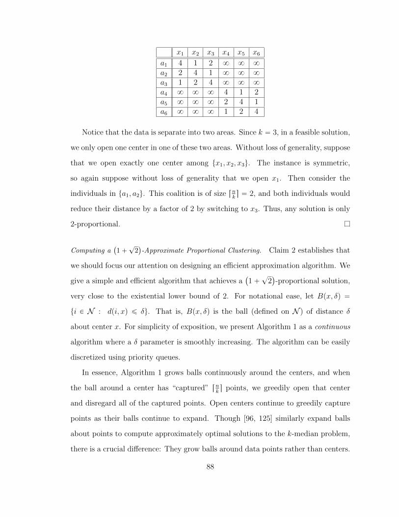
x1 x2 x3 x4 x5 x6
a1 4 1 2 8 8 8
a2 2 4 1 8 8 8
a3 1 2 4 8 8 8
a4 8 8 8 4 1 2a5 8 8 8 2 4 1a6 8 8 8 1 2 4
Notice that the data is separate into two areas. Since k “ 3, in a feasible solution,
we only open one center in one of these two areas. Without loss of generality, suppose
that we open exactly one center among tx1, x2, x3u. The instance is symmetric,
so again suppose without loss of generality that we open x1. Then consider the
individuals in ta1, a2u. This coalition is of size rnks “ 2, and both individuals would
reduce their distance by a factor of 2 by switching to x3. Thus, any solution is only
2-proportional.
Computing a`
1`?
2˘
-Approximate Proportional Clustering. Claim 2 establishes that
we should focus our attention on designing an efficient approximation algorithm. We
give a simple and efficient algorithm that achieves a`
1`?
2˘
-proportional solution,
very close to the existential lower bound of 2. For notational ease, let Bpx, δq “
ti P N : dpi, xq ď δu. That is, Bpx, δq is the ball (defined on N ) of distance δ
about center x. For simplicity of exposition, we present Algorithm 1 as a continuous
algorithm where a δ parameter is smoothly increasing. The algorithm can be easily
discretized using priority queues.
In essence, Algorithm 1 grows balls continuously around the centers, and when
the ball around a center has “captured” rnks points, we greedily open that center
and disregard all of the captured points. Open centers continue to greedily capture
points as their balls continue to expand. Though [96, 125] similarly expand balls
about points to compute approximately optimal solutions to the k-median problem,
there is a crucial difference: They grow balls around data points rather than centers.
88

Algorithm 1 Greedy Capture
1: δ Ð 0; X ÐH; N Ð N2: while N ‰ H do3: Smoothly increase δ4: while Dx P X s.t. |Bpx, δq XN | ě 1 do5: N Ð NzBpx, δq6: while Dx P pMzXq s.t. |Bpx, δq XN | ě rn
ks do
7: X Ð X Y txu8: N Ð NzBpx, δq9: return X
Theorem 12. Algorithm 1 yields a p1`?
2q-proportional clustering, and there exists
an instance for which this bound is tight.
Proof. Let X be the solution computed by Algorithm 1. First note that X uses at
most k centers, since it only opens a center when rnks unmatched points are absorbed
by the ball around that center, and this can happen at most k times. Now, suppose
for a contradiction that X is not a p1 `?
2q-proportional clustering. Then there
exists S Ď N with |S| ě rnks and y PM such that
@i P S, p1`?
2q ¨ dpi, yq ă DipXq. (4.1)
Let ry be the distance of the farthest agent from y in S, that is, ry :“ maxiPS dpi, yq,
and call this agent i˚. There are two cases. In the first case, Bpx, ryqXS “ H for all
x P X. This immediately yields a contradiction, because it implies that Algorithm 1
would have opened y. In particular, note that S Ď Bpy, ryq, so if S X Bpx, ryq “ H
for all x P X, then Bpy, ryq would have had at least rnks unmatched points.
In the second case, Dx P X and Di P N such that i P Bpx, ryq X S. This case
is drawn below in Figure 4.2. By the triangle inequality, dpx, yq ď dpi, xq ` dpi, yq.
Therefore, dpi˚, xq ď ry ` dpi, xq ` dpi, yq. Also, dpi, xq ď ry, since i P Bpx, ryq.
Consider the minimum multiplicative improvement of i and i˚:
89

y x
i˚
ry
i
Figure 4.2: Diagram for Proof of Theorem 12
min
ˆ
dpi, xq
dpi, yq,dpi˚, xq
dpi˚, yq
˙
ď min
ˆ
dpi, xq
dpi, yq,ry ` dpi, xq ` dpi, yq
ry
˙
ď min
ˆ
rydpi, yq
, 2`dpi, yq
ry
˙
ď maxzě0
pmin pz, 2` 1zqq “ 1`?
2
which violates equation 4.1. To see that there exists an instance for which Al-
gorithm 1 yields exactly this bound, consider the following instance with N “
ta1, a2, . . . , a6u, M “ tx1, x2, x3, x4u and k “ 3. Distances are specified in the
following table, where ε ą 0 is some small constant.
x1 x2 x3 x4
a1 1 1`?
2 8 8
a2?
2´ 1 1´ ε 8 8
a3 1`?
2 1´ ε 8 8
a4 8 8 1 1`?
2
a5 8 8?
2´ 1 1´ ε
a6 8 8 1`?
2 1´ ε
The distances satisfy the triangle inequality. Note that Algorithm 1 will open x2 and
x4. The coalition ta1, a2u can each reduce their distance by a multiplicative factor
approaching 1`?
2 as εÑ 0 by deviating to x1.
90

Theorem 12 establishes that constant approximate proportional clusterings al-
ways exist, and can be computed efficiently. However, Algorithm 1 may prove un-
satisfactory, in the sense that it may find an approximate proportional clustering
with poor global objective (e.g., k-median or k-means), even when exact propor-
tional clusterings with good global objectives exist. For example, suppose k “ 2 and
there are two easily defined clusters, one containing 40% of the data and the other
containing 60% of the data. It is possible that Algorithm 1 will only open centers
inside of the larger cluster. This is proportional, but clearly bad on the k-median
and k-means objectives, even with respect to proportional solutions (notice that the
“correct” clustering of such an example is still proportional). In Section 4.3, we show
how to address this concern by optimizing the k-median objective subject to pro-
portionality as a constraint. Later, in Section 4.5, we empirically study the tradeoff
between the k-means objective and proportionality on real data.
4.3 Proportionality as a Constraint
We consider the k-median and k-means objectives to be reasonable measures of the
global quality of a solution. We see minimizing the k-center objective more as a
competing notion of fairness, and so we focus on optimizing the k-median objective
subject to proportionality.2
Minimizing the k-median objective without proportionality is a well studied prob-
lem in approximation algorithms, and several constant approximations are known [43,
13, 125]. Most of this work is in the model where N ĎM, and we follow suit in this
section. We show the following.
Theorem 13. Suppose there is a ρ-proportional clustering with k-median objective
2 A constant approximation algorithm for minimizing the k-median objective immediately impliesa constant approximation algorithm for minimizing the k-means objective by running the algorithmon the squared distances [125].
91
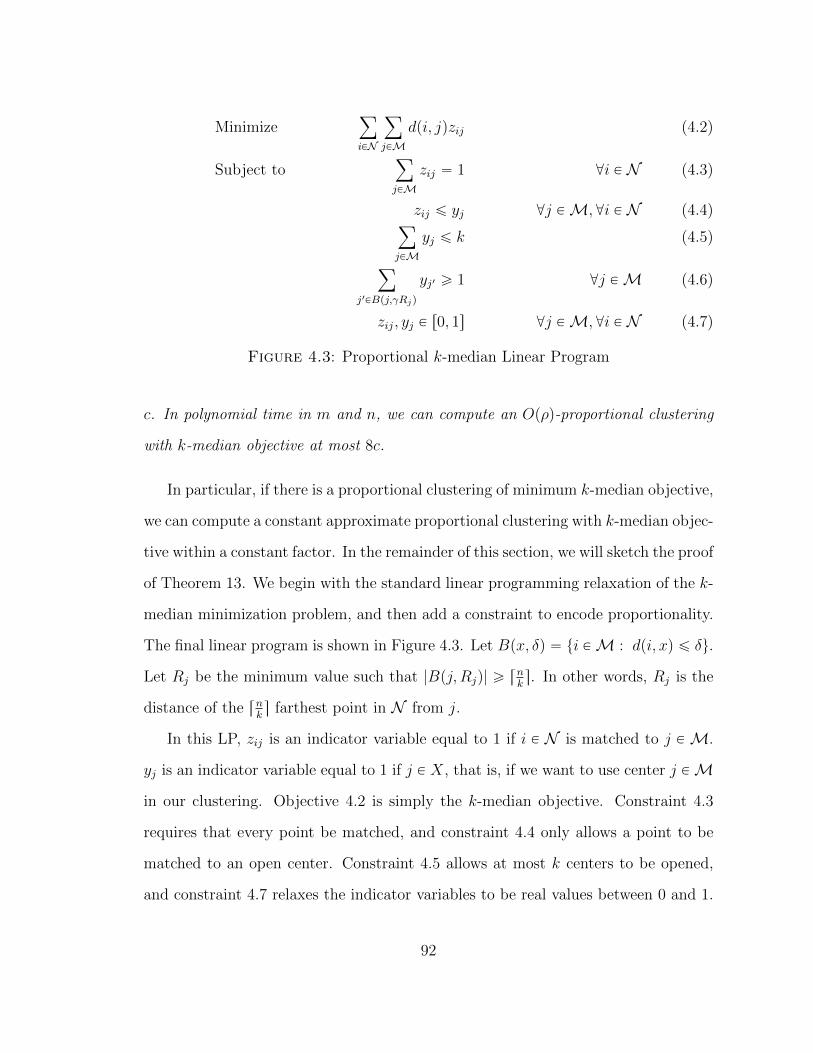
Minimizeÿ
iPN
ÿ
jPMdpi, jqzij (4.2)
Subject toÿ
jPMzij “ 1 @i P N (4.3)
zij ď yj @j PM, @i P N (4.4)ÿ
jPMyj ď k (4.5)
ÿ
j1PBpj,γRjq
yj1 ě 1 @j PM (4.6)
zij, yj P r0, 1s @j PM, @i P N (4.7)
Figure 4.3: Proportional k-median Linear Program
c. In polynomial time in m and n, we can compute an Opρq-proportional clustering
with k-median objective at most 8c.
In particular, if there is a proportional clustering of minimum k-median objective,
we can compute a constant approximate proportional clustering with k-median objec-
tive within a constant factor. In the remainder of this section, we will sketch the proof
of Theorem 13. We begin with the standard linear programming relaxation of the k-
median minimization problem, and then add a constraint to encode proportionality.
The final linear program is shown in Figure 4.3. Let Bpx, δq “ ti PM : dpi, xq ď δu.
Let Rj be the minimum value such that |Bpj, Rjq| ě rnks. In other words, Rj is the
distance of the rnks farthest point in N from j.
In this LP, zij is an indicator variable equal to 1 if i P N is matched to j P M.
yj is an indicator variable equal to 1 if j P X, that is, if we want to use center j PM
in our clustering. Objective 4.2 is simply the k-median objective. Constraint 4.3
requires that every point be matched, and constraint 4.4 only allows a point to be
matched to an open center. Constraint 4.5 allows at most k centers to be opened,
and constraint 4.7 relaxes the indicator variables to be real values between 0 and 1.
92
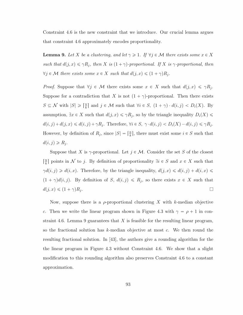
Constraint 4.6 is the new constraint that we introduce. Our crucial lemma argues
that constraint 4.6 approximately encodes proportionality.
Lemma 9. Let X be a clustering, and let γ ě 1. If @j PM there exists some x P X
such that dpj, xq ď γRj, then X is p1` γq-proportional. If X is γ-proportional, then
@j PM there exists some x P X such that dpj, xq ď p1` γqRj.
Proof. Suppose that @j P M there exists some x P X such that dpj, xq ď γRj.
Suppose for a contradiction that X is not p1 ` γq-proportional. Then there exists
S Ď N with |S| ě rnks and j P M such that @i P S, p1 ` γq ¨ dpi, jq ă DipXq. By
assumption, Dx P X such that dpj, xq ď γRj, so by the triangle inequality DipXq ď
dpi, jq`dpj, xq ď dpi, jq`γRj. Therefore, @i P S, γ ¨dpi, jq ă DipXq´dpi, jq ď γRj.
However, by definition of Rj, since |S| “ rnks, there must exist some i P S such that
dpi, jq ě Rj.
Suppose that X is γ-proportional. Let j PM. Consider the set S of the closest
rnks points in N to j. By definition of proportionality Di P S and x P X such that
γdpi, jq ě dpi, xq. Therefore, by the triangle inequality, dpj, xq ď dpi, jq ` dpi, xq ď
p1 ` γqdpi, jq. By definition of S, dpi, jq ď Rj, so there exists x P X such that
dpj, xq ď p1` γqRj.
Now, suppose there is a ρ-proportional clustering X with k-median objective
c. Then we write the linear program shown in Figure 4.3 with γ “ ρ ` 1 in con-
straint 4.6. Lemma 9 guarantees that X is feasible for the resulting linear program,
so the fractional solution has k-median objective at most c. We then round the
resulting fractional solution. In [43], the authors give a rounding algorithm for the
the linear program in Figure 4.3 without Constraint 4.6. We show that a slight
modification to this rounding algorithm also preserves Constraint 4.6 to a constant
approximation.
93
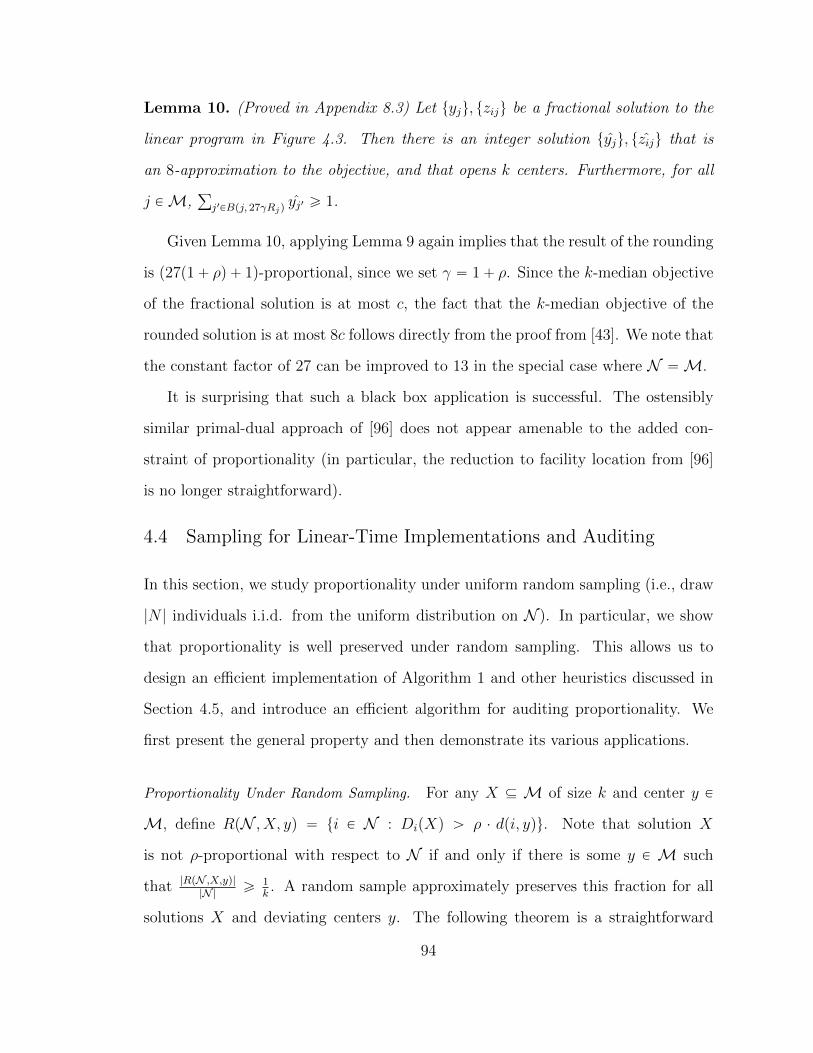
Lemma 10. (Proved in Appendix 8.3) Let tyju, tziju be a fractional solution to the
linear program in Figure 4.3. Then there is an integer solution tyju, tziju that is
an 8-approximation to the objective, and that opens k centers. Furthermore, for all
j PM,ř
j1PBpj, 27γRjqyj1 ě 1.
Given Lemma 10, applying Lemma 9 again implies that the result of the rounding
is p27p1` ρq ` 1q-proportional, since we set γ “ 1` ρ. Since the k-median objective
of the fractional solution is at most c, the fact that the k-median objective of the
rounded solution is at most 8c follows directly from the proof from [43]. We note that
the constant factor of 27 can be improved to 13 in the special case where N “M.
It is surprising that such a black box application is successful. The ostensibly
similar primal-dual approach of [96] does not appear amenable to the added con-
straint of proportionality (in particular, the reduction to facility location from [96]
is no longer straightforward).
4.4 Sampling for Linear-Time Implementations and Auditing
In this section, we study proportionality under uniform random sampling (i.e., draw
|N | individuals i.i.d. from the uniform distribution on N ). In particular, we show
that proportionality is well preserved under random sampling. This allows us to
design an efficient implementation of Algorithm 1 and other heuristics discussed in
Section 4.5, and introduce an efficient algorithm for auditing proportionality. We
first present the general property and then demonstrate its various applications.
Proportionality Under Random Sampling. For any X Ď M of size k and center y P
M, define RpN , X, yq “ ti P N : DipXq ą ρ ¨ dpi, yqu. Note that solution X
is not ρ-proportional with respect to N if and only if there is some y P M such
that |RpN ,X,yq||N | ě 1
k. A random sample approximately preserves this fraction for all
solutions X and deviating centers y. The following theorem is a straightforward
94

consequence of Hoeffding’s inequality. The important idea in the proof is that we
take a union bound over all possible solutions and deviations, and there are only
k`
mk
˘
such combinations.
Theorem 14. Given N , M and parameter ρ ě 1, fix parameters ε, δ P r0, 1s. Let
N Ď N of size Ω´
k3
ε2log m
δ
¯
be chosen uniformly at random. Then, with probability
at least 1´ δ, the following holds for all pX, yq:
ˇ
ˇ
ˇ
ˇ
|RpN,X, yq|
|N |´|RpN , X, yq|
|N |
ˇ
ˇ
ˇ
ˇ
ďε
k
Proof. Recall that N is a random sample of N . Hoeffding’s inequality implies that
for any fixed pX, yq, a sample of size |N | “ O´
1ε2
log 1
δ
¯
is sufficient to achieve
ˇ
ˇ
ˇ
ˇ
|RpN,X, yq|
|N |´|RpN , X, yq|
|N |
ˇ
ˇ
ˇ
ˇ
ď ε
with probability at least 1 ´ δ. Note that there are q “ m`
mk
˘
possible choices of
pX, yq over which we take the union bound. Setting δ “ δq, and ε “ ε
kis sufficient for
the union bound to yield the theorem statement.
In order to apply the above theorem, we say that a solution X is ρ-proportional
to p1 ` εq-deviations if for all y PM and for all S Ď N where |S| ě p1 ` εqnk, there
exists some i P S such that ρ ¨ dpi, yq ě DipXq. Note that if X is ρ-proportional to
1-deviations, it is simply ρ-proportional. We immediately have the following:
Corollary 1. Let N Ă N be a uniform random sample of size |N | “ Ω´
k3
ε2ln m
δ
¯
.
Suppose X Ď M with |X| “ k is ρ-proportional with respect to N . Then with
probability at least 1´ δ, X is ρ-proportional to p1` εq-deviations with respect to N .
95
Linear Time Implementation. We now consider how to take advantage of Theorem 14
to optimize Algorithm 1. To state running times simply, we use the convention that
fpnq is Opgpnqq if fpnq is Opgpnqq up to poly-logarithmic factors. First, note that
Algorithm 1 takes Opmnq time, which is quadratic in input size. A corollary of
Theorem 14 is that we can approximately implement Algorithm 1 in nearly linear
time, comparable to the running time of the standard k-means heuristic.
Corollary 2. Algorithm 1, when run on M and a random sample N Ď N of size
|N | “ Θ´
k3
ε2
¯
, provides a solution that is p1`?
2q-proportional to p1` εq-deviations
with high probability in O´
k3
ε2m¯
time.
Efficient Auditing. Alternatively, one might still want to run one’s favorite clustering
algorithm, e.g., the k-means heuristic, and ask whether the solution produced hap-
pens to be proportional. We call this the Audit Problem. Given N ,M, and X Ă N
with |X| ď k, find the minimum value of ρ such that X is ρ-proportional.
It is not too hard to see that one can solve the Audit Problem exactly in Oppk`
mqnq time by computing for each y P M, the quantity ρy, the rnks largest value of
DipXqdpi,yq
. We subsequently find the y that maximizes ρy. Again, this takes quadratic
time, which can be worse than the time taken to find the clustering itself.
Consider a slightly relaxed pε, δq-Audit Problem where we are asked to find the
minimum value of ρ such that X is ρ-proportional to p1` εq-deviations with proba-
bility at least 1´δ. This problem can be efficiently solved by using a random sample
N Ď N of points to conduct the audit.
Corollary 3. The pε, δq-Audit Problem can be solved in O´
pk `mq k3
ε2
¯
time.
96

4.5 Implementations and Empirical Results
In this section, we study proportionality on real data taken from the UCI Machine
Learning Repository [59]. In particular, we consider three qualitatively different data
sets used for clustering: Iris, Diabetes, and KDD. For each data set, we only have a
single set of points given as input, so we take N “M to be the set of all points in
the data set. We use the standard Euclidean L2 distance.
• Iris. This data set contains information about the petal dimensions of three
different species of iris flowers. There are 50 samples of each species.
• Diabetes. This is the Pima Indians Diabetes data set, and contains information
about 768 diabetes patients, recording features like glucose, blood pressure, age
and skin thickness.
• KDD. This is the KDD cup 1999 data set, containing information about con-
nections of sequences of TCP Packets. Each TCP Packet can classified as
normal or one of twenty-two types of intrusions. Of these 23 classes, normal,
“neptune”, and “smurf” account for 98.3% of the data.3
4.5.1 Local Capture Heuristic
We observe that while our Greedy Capture algorithm (Algorithm 1) always produces
an approximately proportional solution, it may not produce an exactly proportional
solution in practice, even on instances where such solutions exist (see Figure 4.4a
and Figure 4.4b). We therefore introduce a Local Capture heuristic that is able to
consistently outperform Greedy Capture in practice.
3 The data set is extremely large; we work with a subsample of 100,000 points. We run k-means++on this entire 100,000 point sample. For efficiency, we run our Local Capture algorithm by furthersampling 5,000 points uniformly at random to treat as N and sampling 400 points via the k-means++ initialization to treat as M. For the sake of a fair comparison, we generate a differentsample of 400 centers using the k-means++ initialization that we use to determine the value of ρ we
97

Algorithm 2 Local Capture Heuristic
1: Input ρ2: Initialize X as a random subset of k centers from M.3: repeat4: for y PM do5: Sy Ð ti P N : ρ ¨ diy ă DipXqu6: if |Sy| ě rn
ks then
7: x˚ Ð argminxPX |ti P N : dix “ DipXqu|8: X Ð pXztx˚uq Y tyu9: until no changes occur
10: return X
Algorithm 2 searches for violations of ρ-proportionality (note that ρ is a param-
eter), and if it finds one, swaps the least demanded center for the center of the
proposed violation. Every iteration of Algorithm 2 (the entire inner for loop) runs
in Opmn2q time, and n can be reduced via sampling as discussed in Section 4.4. In
our experiments, we try to find the minimum ρ for which the algorithm terminates
in a small number of iterations via binary search over possible input of ρ. If Algo-
rithm 2 terminates, then it returns a ρ-proportional solution. In [13], the authors
also evaluate a local search swapping procedure for the k-median problem, but their
swap condition is based on the relative k-median objective of two solutions, whereas
our swap condition is based on violations to proportionality.
4.5.2 Proportionality and k-means Objective Tradeoff
We compare Greedy Capture (Algorithm 1) and Local Capture (Algorithm 2) with
the k-means++ algorithm (Lloyd’s algorithm for k-means minimization with the k-
means++ initialization [12]) for a range of values of k. For the Iris data set, Local
Capture and k-means++ always find an exact proportional solution (Figure 4.4a),
and have comparable k-means objectives (Figure 4.5a). The Iris data set is very
simple with three natural clusters, and validates the intuition that proportionality
report for both Local Capture and the k-means++ algorithm. The k-means objective is measuredon the original 100,000 points for both algorithms.
98
(a) Iris (b) Diabetes (c) KDD, geometric scale
Figure 4.4: Minimum ρ such that the solution is ρ-proportional
.
(a) Iris (b) Diabetes (c) KDD, geometric scale
Figure 4.5: k-means objective
and the k-means objective are not always opposed.
The Diabetes data set is larger and more complex. As shown in Figure 4.4b,
k-means++ no longer always finds an exact proportional solution. Local Capture
always finds a better than 1.01-proportional solution. As shown in Figure 4.5b, the
k-means objectives of the solutions are separated, although generally on the same
order of magnitude.
The contrast between the k-means objective and proportionality is pronounced for
the KDD data set. Greedy Capture’s performance on this data set is comparable to
Local Capture, so we omit it for clarity. In Figure 4.4c, note that for many values of k,
the k-means++ algorithm only finds a roughly 4,000-proportional clustering. On the
other hand, Local Capture is still consistently able to find a roughly 2-proportional
clustering or better. There is a similarly dramatic difference of between three and
99
five orders of magnitude in the k-means objectives achieved by the algorithms, as
seen in Figure 4.5c. This behavior appears to be due to the presence of significant
outliers in the KDD data set. This is in keeping with the theoretical impossibility
of simultaneously approximating the optima on both objectives, and demonstrates
that this tension arises in practice as well as theory.
Note that if one is allowed to use 2k centers when k is given as input, one can
trivially achieve the proportionality of Local Capture and the k-means objective of
the k-means++ algorithm by taking the union of the two solutions. Thinking in this
way leads to a different way of quantifying the tradeoff between proportionality and
the k-means objective: Given an approximately proportional solution, how many
extra centers are necessary to get comparable k-means objective as the k-means++
algorithm? For a given data set, the answer is a value between 0 and k, where larger
numbers indicate more incompatibility, and lower numbers indicate less incompati-
bility.
We consider this question by first computing the union of centers computed by
Local Capture and the k-means++ algorithm. We then greedily remove centers
as long as doing so does not increase the minimum ρ such that the solution is ρ-
proportional (defined on k, not 2k) by more than a multiplicative factor of α, and
does not increase the k-means objective by more than a multiplicative factor β.
On the KDD dataset, we set α “ 1.2 and β “ 1.5, so the proportionality of the
result is within 1.2 of Local Capture in Figure 4.4c, and the k-means objective is
within 1.5 of k-means++ in Figure 4.5c. We observe that this heuristic uses at most
3 extra centers for any k ď 10. So while there is real tension between proportionality
and the k-means objective, this tension is still not maximal. In the worst case, one
might need to add k centers to a proportional solution to compete with the k-means
objective of the k-means++ algorithm, but in practice we find that we need at most
3 for k ď 10.
100

4.6 Conclusion and Open Directions
We have introduced proportionality as a fair solution concept for centroid clustering.
Although exact proportional solutions may not exist, we gave efficient algorithms
for computing approximate proportional solutions, and considered constrained opti-
mization and sampling for further applications. Finally, we studied proportionality
on real data and observed a data dependent tradeoff between proportionality and
the k-means objective. While this tradeoff is in some sense a negative result, it also
demonstrates that proportionality as a fairness guarantee matters in the sense that
it meaningfully constrains the space of solutions.
We have shown that ρ-proportional solutions need not exist for ρ ă 2, and always
exist for ρ ě 1 `?
2. Closing this approximability gap is one outstanding question.
Another is whether there is a more efficient and easily interpretable algorithm for op-
timizing total cost subject to proportionality, as our approach in Section 4.3 requires
solving a linear program on the entire data set. We would ideally like a more efficient
and easily interpretable primal-dual or local search type algorithm. More generally,
what other fair solution concepts for clustering should be considered alongside pro-
portionality, and can we characterize their relative advantages and disadvantages?
Finally, can the idea of proportionality as a group fairness concept be adapted for
supervised learning tasks like classification and regression?
101

5
Metric Implicit Utilitarian Voting via Bargaining
Here, we study social choice: informally, how to pick a point from a decision space
that represents the common good of society. The canonical example is voting. In
that case, the decision space is usually a small set of candidates, and the agents
comprising the society express only ordinal preferences over these candidates. In
contrast, we will study large and complex decision spaces under the implicit utili-
tarian assumption that agents have cardinal preferences over decision points, even
if they cannot concisely express those preferences. The parallel to previous chapters
should now be clear: decision points are public goods and our budget allows us to
choose exactly one good. Intuitively this seems simpler, but we will make severe
restrictions on the kind of input information that agents can provide (note that we
elicited full utility functions in previous sections) in order to develop a practical
mechanism for social choice. Technically, we provide a novel connection between the
concept of Nash bargaining in cooperative game theory and the median of a set of
points in a median graph, and use this connection to design a simple randomized
mechanism that approximately maximizes the utilitarian social welfare. The analy-
sis is over a Markov chain on a hypercube. We also provide several lower bounds,
102
analyze higher moments of the utilitarian social welfare, and show how the results
change in general metric spaces.
Acknowledgements. These results are published in [65], which is joint work with
Ashish Goel, Kamesh Munagala, and Sukolsak Sakshuwong.
5.1 Introduction
Suppose a university administrator plans to spend millions of dollars to update her
campus, and she want to elicit the input of students, staff, and faculty. In a typical
social choice setting, she could first elicit the favorite decisions, or bliss points, of
the students, say “new gym,” “new library,” and “new student center.” However,
voting on these options need not find the social optimum, because it is not clear
that the social optimum is even on the ballot. In such a setting, deliberation be-
tween individuals would find entirely new alternatives, for example “replace gym
equipment plus remodeling campus dining plus money for scholarship”. This leads
to finding a social optimum over a wider space of semi-structured outcomes that the
system/mechanism designer was not originally aware of, and the participants had
not initially articulated.
We therefore start with the following premise: The mechanism designer may not
be able to enumerate the outcomes in the decision space or know their structure, and
this decision space may be too big for most ordinal voting schemes. (For instance,
ordinal voting is difficult to implement in complex combinatorial spaces [114] or in
continuous spaces [75].) However, we assume that agents can still reason about their
preferences and small groups of agents can negotiate over this space and collabora-
tively propose outcomes that appeal to all of them. Our goal is to design protocols
based on such a primitive by which small group negotiation can lead to an aggrega-
tion of societal preferences without a need to formally articulate the entire decision
103
space and without every agent having to report ordinal rankings over this space.
The need for small groups is motivated by a practical consideration as well as
a theoretical one. On the practical side, there is no online platform, to the best of
our knowledge, that has a successful history of large scale deliberation and decision
making on complex issues; in fact, large online forums typically degenerate into vitriol
and name calling when there is substantive disagreement among the participants.
Thus, if we are to develop practical tools for decision making at scale, a sequence of
small group deliberations appears to be the most plausible path. On the theoretical
side, we understand the connections between sequential protocols for deliberation
and axiomatic theories of bargaining for small groups, e.g. for pairs [146, 28], but
not for large groups, and we seek to bridge this gap.
Summary of Contributions. Our main contributions are two-fold:
• A simple and practical sequential protocol that only requires agents to negotiate
in pairs and collaboratively propose outcomes that appeal to both of them.
• A canonical analytic model in which we can precisely state properties of this
protocol in terms of approximation of the social optimum, Pareto-efficiency,
and incentive-compatibility, as well as compare it with simpler protocols.
5.1.1 Background: Bargaining Theory
Before proceeding further, we review bargaining, the classical framework for two
player negotiation in Economics. Two-person bargaining, as framed in [130], is a
game wherein there is a disagreement outcome and two agents must cooperate to
reach a decision; failure to cooperate results in the adoption of the disagreement
outcome. Nash postulated four axioms that the bargaining solution ought to satisfy
assuming a convex space of alternatives: Pareto optimality (agents find an out-
come that cannot be simultaneously improved for both of them), symmetry between
104

agents, invariance with respect to affine transformations of utility (scalar multipli-
cation or additive translation of any agent’s utility should not change the outcome),
and independence of irrelevant alternatives (informally that the presence of a feasible
outcome that agents do not select does not influence their decision). Nash proved
that the solution maximizing the Nash product (that we describe later) is the unique
solution satisfying these axioms. To provide some explanation of how two agents
might find such a solution, [146] shows that Nash’s solution is the subgame perfect
equilibrium of a simple repeated game on the two agents, where the agents take turns
making offers, and at each round, there is an exogenous probability of the process
terminating with no agreement.
The two-person bargaining model is therefore clean and easy to reason about.
As a consequence, it has been extensively studied. In fact, there are other models
and solutions to two-person bargaining, each with a slightly different axiomatiza-
tion [103, 104, 127], as well as several experimental studies [145, 131, 29]. In a social
choice setting, there are typically many more than two agents, each agent having
their own complex preferences. Though bargaining can be generalized to n agents
with similar axiomatization and solution structure, such a generalization is consid-
ered impractical. This is because in reality it is difficult to get a large number of
individuals to negotiate coherently; complexities come with the formation of coali-
tions and power structures [90, 110]. Any model for simultaneous bargaining, even
with three players [26], needs to take these messy aspects into account.
5.1.2 A Practical Compromise: Sequential Pairwise Deliberation
We take a middle path, avoiding both the complexity of explicitly specifying pref-
erences in a large decision space (fully centralized voting), and that of simultaneous
n-person bargaining (a fully decentralized cooperative game). We term this approach
sequential deliberation. We use 2-person bargaining as a basic primitive, and view
105

deliberation as a sequence of pairwise interactions that refine good alternatives into
better ones as time goes by. Our framework has the advantage of being simple with
low cognitive overhead, and is easy to implement and reason about.
More formally, there is a decision space S of feasible alternatives (these may be
projects, sets of projects, or continuous allocations) and a set N of agents. We
assume each agent has a hidden cardinal utility for each alternative. We encapsulate
deliberation as a sequential process. Let H denote the distribution over S generated
by sequential deliberation. We define a bargaining function Bpu, v, aq that takes as
input a pair of agents u and v and a default alternative a. The agents negotiate and
output a consensus alternative o P S; if no consensus is reached then a is output. We
assume Bpu, v, aq satisfies the axioms – symmetry, scale-invariance, independence of
irrelevant alternatives, and Pareto-efficiency – that correspond to Nash bargaining.
Our mechanism is defined in Figure 5.1.
Let a1 be the bliss point of an agent chosen uniformly at random.
1. In each round t “ 1, 2, . . . , T :
(a) A pair of agents ut and vt are chosen independently anduniformly at random with replacement.
(b) These agents are presented with a disagreement alternativeat, and perform Bput, vt, atq as described below.
(c) Agents ut and vt are asked to output a consensus alternative;if they fail to reach a consensus within a specified time frame,the alternative at is output.
(d) Let ot denote the alternative that is output in round t. Weset at`1 “ ot, where we assume a1 is the bliss point of anarbitrary agent.
2. The final social choice is aT . Note that this is equivalent to draw-ing an outcome at random from the distribution generated byrepeating this protocol several times.
Figure 5.1: A framework for sequential pairwise deliberation.
106

5.1.3 Analytical Model: Median Graphs and Sequential Nash Bargaining
The framework in Figure 5.1 is well-defined and practical irrespective of an analytical
model. However, we provide a simple analytical model for specifying the preferences
of the agents in which we can precisely quantify the behavior of this framework as
justification. Assuming that disutility is some metric over the space [7] seems rea-
sonable enough, and our tightest results are for a median graph metrics specifically.
Assume that the set S of alternatives are vertices of a median graph. A median graph
has the property that for each triplet of vertices u, v, w, there is a unique point that
is common to the three sets of shortest paths, those between u, v, between v, w, and
between u,w. This point is the unique median of u, v, w. We assume each agent u
has a bliss point pu P S, and his disutility for an alternative a P S is simply dppu, aq,
where dp¨q is the shortest path distance function on the median graph. (Note that
this disutility can have an agent-dependent scale factor.)
Several natural graphs are median graphs, including trees, points on the line,
hypercubes, and grid graphs in arbitrary dimensions [108]. Median graphs have
been extensively studied as structured models for spatial preferences in voting the-
ory. They are appealing for a very simple reason [48]: For any set of agents and
alternatives on a median graph, if the agents could perform ordinal voting on the al-
ternatives, then the Condorcet winner (an alternative that beats all others in pairwise
voting) always exists, and coincides with the generalized 1-median (the alternative
that minimizes the sum of distances to the agents’ bliss points). In a sense, we con-
sider spaces where had the agents been able to vote, there would have been a clear
winner even using pairwise comparisons. Our premise is that the space is so large
that (a) voting over all possible alternatives is often impractical, and (b) it is not
obvious how to find a small set of “good” alternatives. We therefore ask the natural
questions:
107
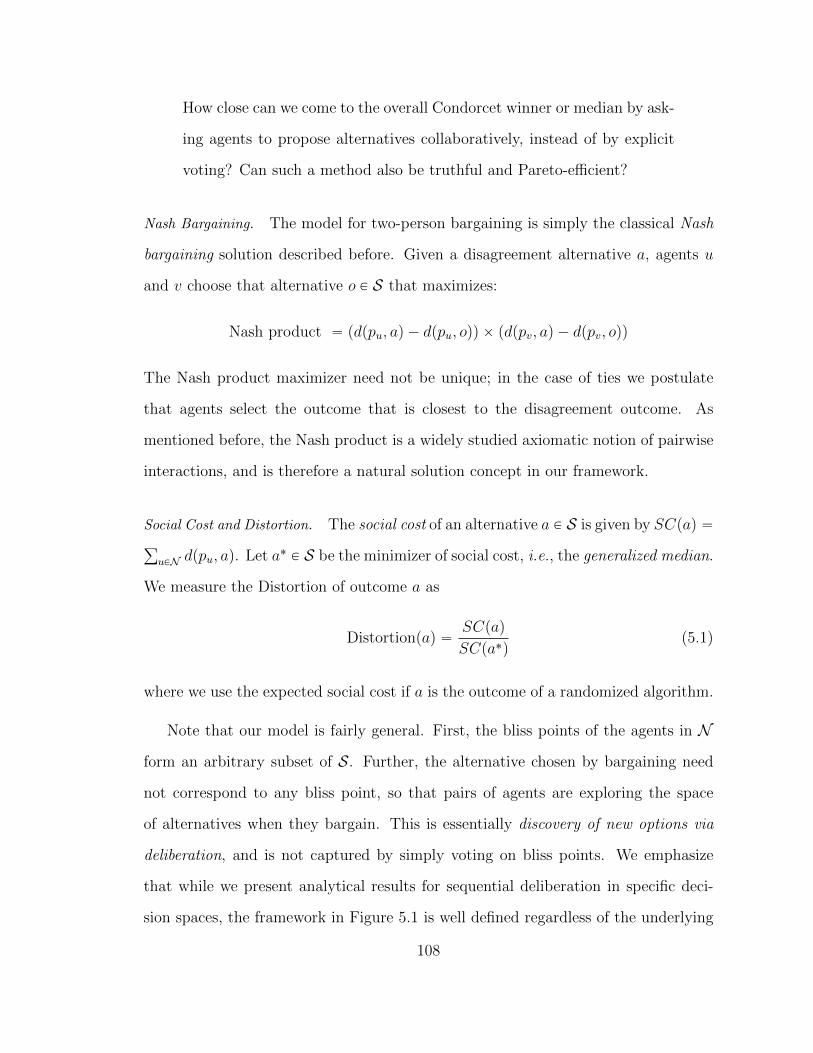
How close can we come to the overall Condorcet winner or median by ask-
ing agents to propose alternatives collaboratively, instead of by explicit
voting? Can such a method also be truthful and Pareto-efficient?
Nash Bargaining. The model for two-person bargaining is simply the classical Nash
bargaining solution described before. Given a disagreement alternative a, agents u
and v choose that alternative o P S that maximizes:
Nash product “ pdppu, aq ´ dppu, oqq ˆ pdppv, aq ´ dppv, oqq
The Nash product maximizer need not be unique; in the case of ties we postulate
that agents select the outcome that is closest to the disagreement outcome. As
mentioned before, the Nash product is a widely studied axiomatic notion of pairwise
interactions, and is therefore a natural solution concept in our framework.
Social Cost and Distortion. The social cost of an alternative a P S is given by SCpaq “ř
uPN dppu, aq. Let a˚ P S be the minimizer of social cost, i.e., the generalized median.
We measure the Distortion of outcome a as
Distortionpaq “SCpaq
SCpa˚q(5.1)
where we use the expected social cost if a is the outcome of a randomized algorithm.
Note that our model is fairly general. First, the bliss points of the agents in N
form an arbitrary subset of S. Further, the alternative chosen by bargaining need
not correspond to any bliss point, so that pairs of agents are exploring the space
of alternatives when they bargain. This is essentially discovery of new options via
deliberation, and is not captured by simply voting on bliss points. We emphasize
that while we present analytical results for sequential deliberation in specific deci-
sion spaces, the framework in Figure 5.1 is well defined regardless of the underlying
108

decision space and the mediator’s understanding of the space. At a high level, this
flexibility and generality in practice are its key advantages.
5.2 Median Graphs and Nash Bargaining
In this section we will use the notation N for a set of agents, S for the space of
feasible alternatives, and H for a distribution over S. Most of our results are for the
analytic model given earlier wherein the set S of alternatives are vertices of a median
graph; see Figure 5.2 for some examples.
Definition 14. A median graph GpS, Eq is an undirected graph with the following
property: For each triplet of vertices u, v, w P S ˆ S ˆ S, there is a unique point
that is common to the shortest paths (which need not be unique between a given pair)
between u, v, between v, w, and between u,w. This point is the unique median of
u, v, w.
Figure 5.2: Examples of Median Graphs
In the framework of Figure 5.1, we assume that at every step, two agents perform
Nash bargaining with a disagreement alternative. The first results characterize Nash
bargaining on a median graph. In particular, we show that Nash bargaining at each
step will select the median of bliss points of the two agents and the disagreement
alternative. After that, we show that we can analyze the Distortion of sequential
deliberation on a median graph by looking at the embedding of that graph onto the
hypercube.
109

Lemma 11. For any median graph G “ pS, Eq, any two agents u, v with bliss points
pu, pv P S, and any disagreement outcome a P S, let M be the median. Then M
maximizes the Nash product of u and v given a, and is the maximizer closest to a.
Proof. Since G is a median graph, M exists and is unique; it must by definition be
the intersection of the three shortest paths between ppu, pvq, ppu, aq, ppv, aq. Note that
we can therefore write dppu, aq “ dppu,Mq ` dpM,aq and similarly for dppv, aq. Let
α “ dppu,Mq; β “ dppv,Mq; and γ “ dpa,Mq. Suppose Nash bargaining finds an
outcome o˚ P S. Let x “ dpo˚, puq and y “ dpo˚, pvq. Observing that M lies on the
shortest path between pu and pv, and using the triangle inequality, we obtain that
x` y ě α ` β.
Noting that dppu, aq “ α` γ and dppv, aq “ β ` γ, the Nash product of the point
o˚ is:
pα ` γ ´ xq ˆ pβ ` γ ´ yq ď pα ` γ ´ xqpγ ´ pα ´ xqq “ γ2 ´ pα ´ xq2
This is maximized when x “ α and y “ β. One possible maximizer is therefore the
point o˚ “ M . Suppose dpo˚, aq ă γ, then by triangle inequality, dppu, o˚q ą α, and
similarly dppv, o˚q ą β. Therefore, there cannot be a closer maximizer of the Nash
product to a than the point M .
Hypercube Embeddings. For any median graph G “ pS, Eq, there is an isometric
embedding φ : GÑ Q of G into a hypercube Q [108]. This embedding maps vertices
S into a subset of vertices of Q so that all pairwise distances between vertices in S
are preserved by the embedding. A simple example of this embedding for a tree is
shown in Figure 5.3. We use this embedding to show the following result.
Lemma 12. Let GpS, Eq be a median graph, and let φ be its isometric embedding
into hypercube QpV,E 1q. For any three points t, u, v P S, let MG be the median
110

Figure 5.3: The hypercube embedding of a 4-vertex star graph
of vertices t, u, v and let MQ be the median of vertices φptq, φpuq, φpvq P V . Then
φpMGq “MQ.
Proof. By definition, since φ is an isometric embedding [108],
dpx, yq “ dpφpxq, φpyqq for all x, y P S (5.2)
Since G is a median graph, MG is the unique median of t, u, v P S, which by definition
satisfies the equalities dpt, uq “ dpt,MGq ` dpMG, uq, dpt, vq “ dpt,MGq ` dpMG, vq,
and dpu, vq “ dpu,MGq ` dpMG, vq.
QpV,E 1q is a hypercube, and is thus also a median graph, so MQ is the unique
median of φptq, φpuq, φpvq P V , which by definition satisfies the equalities
I dpφptq, φpuqq “ dpφptq,MQq ` dpMQ, φpuqq
II dpφptq, φpvqq “ dpφptq,MQq ` dpMQ, φpvqq
III dpφpuq, φpvqq “ dpφpuq,MQq ` dpMQ, φpvqq
Applying Equation (5.2) to the first set of equalities shows that φpMGq satisfies
equalities I,II, and III respectively. But φpMGq P V and MQ is the unique vertex in
V satisfying equalities I,II, and III. Therefore, φpMGq “MQ.
5.3 The Efficiency of Sequential Deliberation
In this section, we show that the Distortion of sequential deliberation is at most
1.208. We then show that this bound is significant, meaning that mechanisms from
simpler classes are necessarily constrained to have higher Distortion values.
111

Upper Bounding Distortion Recall the framework for sequential deliberation in Fig-
ure 5.1 and the definition of Distortion in Equation (5.1). We first map the problem
into a problem on hypercubes using Lemma 12.
Corollary 4. Let G “ pS, Eq be a median graph, let φ : G Ñ Q be an isometric
embedding of G onto a hypercube QpV,E 1q, and let N be a set of agents such that
each agent u has a bliss point pu P S. Then the Distortion of sequential deliberation
on G is at most the Distortion of sequential deliberation on φpGq where each agent’s
bliss point is φppuq.
Proof. Fix an initial disagreement outcome a1 P S and an arbitrary list of T pairs
of agents pu1, v1q, pu2, v2q, . . . , puT , vT q. In round 1 bargaining on G, Lemma 11 im-
plies that sequential deliberation will select o1 “ medianpa1, p1u, p1vq. Furthermore,
Lemma 12 implies that if we had considered φpGq and bargaining on φpa1q, φpp1uq, φpp1vq
instead, sequential deliberation would have selected φpo1q. Suppose at some round t
that we have a disagreement outcome at. Then the same argument yields that if ot
is the bargaining outcome on G, φpotq would have been the bargaining outcome on
φpGq. Thus, by induction, we have that if the list of outcomes on G is o1, ..., oT then
the list of outcomes on φpGq is φpo1q, ..., φpoT q. But recall that φp¨q is an isometric
embedding and the social cost of an alternative is just its sum of distances to all
points in N , so aT and φpaT q have the same social cost.
Furthermore, let a˚ P S denote the generalized median of N . Then, φpa˚q has
the same social cost as a˚. This means the median of the embedding of N into Q
has at most this social cost, which in turn means that the Distortion of sequential
deliberation in the embedding cannot decrease.
Our main result in this section shows that as tÑ 8, the Distortion of sequential
deliberation approaches 1.208, with the convergence rate being exponentially fast in
t and independent of the number of agents |N |, the size of the median space |S|, and
112

the initial disagreement point a1. In particular, the Distortion is at most 1.22 in at
most 9 steps of deliberation, which is indeed a very small number of steps!
Theorem 15. Sequential deliberation among a set N of agents, where the decision
space S is a median graph, yields ErDistortionpatqs ď 1.208` 62t
.
Proof. By Corollary 4, we can assume the decision space is a D-dimensional hyper-
cube Q so that decision points (and thus bliss points) are vectors in t0, 1uD. For
every dimension k, let fk be the fraction of agents whose bliss point has a 1 in the
kth dimension, and let pu,k be the 0 or 1 bit in the kth dimension of the bliss point
pu for agent u. Let a˚ P t0, 1uD be the minimum social cost decision point, i.e.,
a˚ :“ argminaPQSCpaq. Clearly, a˚k is 1 if fk ą 12 and 0 otherwise, so for every
dimension k, the total distance to a˚k, summed over N is:
ÿ
uPN|a˚k ´ pu,k| “ |N |mintfk, 1´ fku
Now, note that sequential deliberation defines a Markov chain on Q. The state in
a given step is just at, and the randomness is in the random draw of the two agents.
Let H˚ be the stationary distribution of the Markov chain. Then we can write
limtÑ8
ErDistortionpatqs “ EaPH˚ rDistortionpaqs
To write down the transition probabilities, we assume this random draw is two
independent uniform random draws from N , with replacement. We also note that
Lemma 11 implies that on Q, sequential deliberation will pick the median in every
step, i.e., given a disagreement outcome at and two randomly drawn agents with bliss
points pu, pv, the new decision point will be ot “ medianppu, pv, atq. On a hypercube,
the median of three points is just the dimension-wise majority. Thus, we get a 2-state
Markov chain in each dimension k, with transition probabilities
Prrotk “ 1|atk “ 1s “ f 2k ` 2fkp1´ fkq and Prrotk “ 1|atk “ 0s “ f 2
k
113

Let P˚k “ limtÑ8 Prrotk “ 1s, and let H˚k denote this stationary distribution for the
corresponding 2-state Markov chain. Then,
P˚k “`
2fk ´ f2k
˘
P˚k ``
f 2k
˘
p1´ P˚k q ñ P˚k “f 2k
1` 2f 2k ´ 2fk
By linearity of expectation, the total expected distance for every dimension k, summed
over u P N to the final outcome is given by
EakPH˚k
«
ÿ
uPN|ak ´ pu,k|
ff
“ |N |ˆˆ
f 2k
f 2k ` p1´ fkq
2
˙
p1´ fkq `
ˆ
1´f 2k
f 2k ` p1´ fkq
2
˙
fk
˙
“ |N |ˆ
fkp1´ fkq
f 2k ` p1´ fkq
2
˙
Without loss of generality, let fk P r0, 12s so that for dimension k, the total distance
to a˚k is |N |fk. Then the ratio of the expected total distance to H˚k to the total
distance to a˚k is at most:
EakPH˚k rř
uPN |pu,k ´ ak|sř
uPN |pu,k ´ a˚k|
ď maxfkPr0,12s1´ fk
f 2k ` p1´ fkq
2ď 1.208
Since the above bound holds in each dimension of the hypercube, we can combine
them as:
EaPH˚ rDistortionpaqs “
řDk“1 EakPH˚k r
ř
uPN |pu,k ´ ak|sřDk“1
ř
uPN |pu,k ´ a˚k|
ď 1.208
Now that we have bounded the Distortion of the stationary distribution, we need
to consider the convergence rate. We will not bound the mixing time of the overall
Markov chain. Rather, note that in the preceding analysis, we only used the marginal
probabilities H˚k for each dimension k. Furthermore, the Markov chain defined by
114

sequential deliberation need not walk along edges on Q, so we can consider separately
the convergence of the chain to the stationary marginal in each dimension.
After t steps, let Pkt “ Prrotk “ 1s and let Htk denote this distribution. Assume
fk P r0, 12s. If the total variation distance between Htk and H˚
k is εf2k
f2k`p1´fkq2 , then
it is easy to check that the expected total distance to Htk is within a p1 ` εq factor
of the expected distance to H˚k , which implies a Distortion of at most 1.208 ` ε
in that dimension. We therefore bound how many steps it takes to achieve total
variation distance εf2k
f2k`p1´fkq2 in any dimension k; if this bound holds uniformly
for all dimensions k, this would imply the overall Distortion is at most 1.208 ` ε,
completing the proof.
For any dimension k, two executions of the 2-state Markov chain along that
dimension couple if the agents picked in a time step have the same value in that
dimension. At any step, this happens with probability at least pf 2k ` p1´ fkq
2q.
Therefore, the probability that the chains have not coupled in t steps is at most
`
1´`
f 2k ` p1´ fkq
2˘˘t“ p2fkp1´ fkqq
t
We therefore need T large enough so that
p2fkp1´ fkqqTď ε
f2kf2k`p1´fkq
2
ñ T “ maxfkPr0,12s
ˆ
log 1ε
log 12fkp1´fkq
`log 1
f2k
`logpf2k`p1´fkq2q
log 12fkp1´fkq
˙
ñ T ď log21ε` 2.575
Since this bound of T holds uniformly for all dimensions, this directly implies the
theorem.
5.3.1 Lower Bounds on Distortion
We will now show that the Distortion bounds of sequential deliberation are signifi-
cant, meaning that mechanisms from simpler classes are constrained to have higher
115

Distortion values. We present a sequence of lower bounds for social choice mecha-
nisms that are restricted to use increasingly richer information about the space of
alternatives on a median graph G “ pS, Eq with a set of agents N with bliss points
VN Ď S. We first consider mechanisms that are constrained to choose outcomes in
VN . For instance, this captures the random dictatorship that chooses the bliss point
of a random agent as the final outcome. It shows that the compromise alternatives
found by deliberation do play a role in reducing Distortion.
Lemma 13. Any mechanism constrained to choose outcomes in VN has Distortion
at least 2.
Proof. It is easy to see that the k-star graph (the graph with a central vertex con-
nected to k other vertices none of which have edges between themselves) is a median
graph. Consider an |N |-star graph where VN are the non central vertices; that is,
each and every agent has a unique bliss point on the periphery of the star. Then any
mechanism constrained to choose outcomes in VN must choose one of these vertices
on the periphery of the star. The social cost of such a point is p|N |´ 1qˆ 2, whereas
the social cost of the optimal central vertex is clearly just |N |. The Distortion goes
to 2 as |N | grows large.
We next consider mechanisms that are restricted to choosing the median of the
bliss points of some three agents in N . In particular, this captures sequential delib-
eration run for T “ 1 steps, as well as mechanisms that generalize dictatorship to
an oligarchy composed of at most 3 agents. This shows that iteratively refining the
bargaining outcome has better Distortion than performing only one iteration.
Lemma 14. Any mechanism constrained to choose outcomes in VN or a median of
three points in VN must have Distortion at least 1.316.
Proof. Let G be a median graph; in particular let G be the D-dimensional hypercube
t0, 1uD. For every dimension, an agent has a 1 in that dimension of their bliss point
116

independently with probability p. In expectation p|N | agents’ bliss points have a 1 in
any given dimension. We assume 0 ă p ă 12 is an absolute constant. For a˚ being
the all 0’s vector, ErSCpa˚qs “ D|N |p, where the randomness is in the construction.
Now, suppose D “ polylogp|N |q. Then, for any β ă 1, with probability at least
1 ´ 1
polyp|N |qevery three points in VN has at least βp3p2 ´ 2p3qD ones. By union
bounds, for some α P pβ, 1q, the social cost of any median of three points in VN is at
least:
ErSCpaqs ě D|N |α“
p3p2 ´ 2p3qp1´ pq ` pp1´ 3p2 ` 2p3q‰
“ D|N |α`
4p4 ´ 8p3 ` 3p2 ` p˘
where again, the randomness is in the construction. Then there is nonzero probability
that
ErSCpaqsErSCpa˚qs
ě α`
4p3 ´ 8p2 ` 3p` 1˘
(5.3)
If we choose the argmax of Equation 5.3, we get nonzero probability over the con-
struction that the Distortion is at least p1.316qα. Letting α grow close to 1 and
noting that the nonzero probability over the construction implies the existence of
one such instance completes the argument.
We finally consider a class of mechanisms that includes sequential deliberation
as a special case. We show that any mechanism in this class cannot have Distortion
arbitrarily close to 1. This also shows that sequential deliberation is close to best
possible in this class.
Lemma 15. Any mechanism constrained to choose outcomes on shortest paths be-
tween pairs of outcomes in VN must have Distortion at least 98 “ 1.125.
Proof. The construction of the lower bound essentially mimics that of Lemma 14.
In this case however, we get that each point on a shortest path between two agents
117

has at least αpp2 ˆ p1´ pq ` p1´ p2q ˆ pqD ones, so
ErSCpaqs ě D|N |α“
p2 ˆ p1´ pq ` p1´ p2q ˆ p‰
“ D|N |α`
´2p3 ` p2 ` p˘
So there is nonzero probability over the construction that
ErSCpaqsErSCpa˚qs
ě α`
´2p2 ` p` 1˘
where the maximum of ´2p2 ` p ` 1 over p ă 12 is 98 when p “ 14. The rest of
the argument follows as in Lemma 14.
The significance of the lower bound in Lemma 15 should be emphasized: though
there is always a Condorcet winner in median graphs, it need not be any agents bliss
point, nor does it need to be Pareto optimal for any pair of agents. The somewhat
surprising implication is that any local mechanism (in the sense that the mechanism
chooses locally Pareto optimal points) is constrained away from finding the Condorcet
winner. At first glance, it might seem like [82] violates this lower bound; but it is
crucial to note that in their model, the decision space consists only of the bliss points
of agents, rather than being a potentially much larger superset.
5.4 Properties of Sequential Deliberation
In this section, we study some natural desiderata that should be satisfied by reason-
able social choice functions, and ask if Sequential Deliberation satisfies them.
Pareto-Efficiency We first show that the outcome of sequential deliberation is ex-
post Pareto-efficient on a median graph. In other words, in any realization of the
random process, suppose the final outcome is o; then there is no other alternative a
such that dpa, vq ď dpo, vq for every v P N , with at least one inequality being strict.
This is a weak notion of efficiency, but it is not trivial to show; while it is easy to
118

see that a one shot bargaining mechanism using only bliss points is Pareto efficient
by virtue of the Pareto efficiency of bargaining, sequential deliberation defines a
potentially complicated Markov chain for which many of the outcomes need not be
bliss points themselves.
Theorem 16. Sequential deliberation among a set N of agents, where the decision
space S is a median graph and the initial disagreement point a1 is the bliss point of
some agent, yields an ex-post Pareto Efficient alternative.
Proof. Let G “ pS, Eq be a median graph, let N be a set of agents, and let VN Ď S
be the set of bliss points of the agents in N . It follows from the proof of Corollary 4
that without loss of generality we can suppose S is a hypercube embedding.
Consider some realization px1, y1q, px2, y2q, ..., pxT , yT q of sequential bargaining,
where pxt, ytq P S are the bliss points of the agents drawn to bargain in step t.
Let oT denote the final outcome. For the sake of contradiction assume there is an
alternative z that Pareto-dominates oT , i.e., dpz, vq ď dpoT , vq for each v P N , with
at least one inequality being strict.
Recall that on the hypercube, the median of three points has the particularly
simple form of the dimension wise majority. Let Kt be the set of dimensions of the
hypercube S that are “decided” by the agents in round t in the sense that these agents
agree on that dimension (and can thus ignore the outside alternative in that dimen-
sion) and all future agents disagree on that dimension (and thus keep the value de-
cided by bargaining in round t). Formally, Kt “
k : xtk “ ytk and @t1 ą t, xt1
k ‰ yt1
k
(
.
Then by the majority property of the median on the hypercube, for any dimension
k such that k P Kt for some t P t1, . . . , T u, it must be that oTk “ xtk. An example is
shown in Figure 5.4.
Consider the final round T . It must be that @k P KT , zk “ oTk . If this were not
the case, z would not be pairwise efficient (i.e., on a shortest path from xT to yT ),
119

VN 01100101000000111000
t xt
ytat!ot
Kt
1 1010000001
01100!
001002
2 1010011000
00100!
101005
3 0000101100
10100!
00100∅
4 0110000001
00100!
001001,4
Figure 5.4: An example of sequential deliberation with Kt labeled. The dimensionsare numbered 1, 2, . . . , 5.
whereas oT is pairwise efficient by definition of the median, so one of the agents in
round T would strictly prefer oT to z, violating the dominance of z over oT .
Next, consider round T ´ 1. Partition the dimensions of S into KT ,KT´1 and
all others. Suppose for a contradiction that Dk P KT´1 such that zk ‰ oTk , where
xT´1k “ yT´1 “ oTk by definition. Then the agents in round T ´ 1 must strictly prefer
oT to z on the dimensions in KT´1. But for k P KT , we know that zk “ oTk , so the
agents are indifferent between z and oT on the dimensions in KT . Furthermore, for
k R KT YKT´1, xT´1k ‰ yT´1k , so at least one of the two agents at least weakly prefers
oT to z on the remaining dimensions. But then at least one agent must strictly prefer
oT to z, contradicting the dominance of z over oT .
Repeating this argument yields that for all k P K1 Y K2 Y . . . Y KT , zk “ oTk .
For all other dimensions, oTk takes on the value a1, which is the bliss point of some
agent. Since that agent must weakly prefer z to oT , z must also take the value of her
bliss point on these remaining dimensions. But then z “ oT , so z does not Pareto
dominate oT , a contradiction.
Uniqueness of Stationary Distribution Next, we show that the Markov chain corre-
sponding to sequential deliberation converges to a unique stationary distribution on
120

the actual median graph, rather than just showing that the marginals and thus the
expected distances from the perspectives of the agents converge.
Theorem 17. The Markov chain defined in Theorem 15 has a unique stationary
distribution.
Proof. It is helpful to note that the Markov chain defined by sequential bargaining on
G by N only puts nonzero probability mass on points in the median closure MpVN q
of VN (see Definition 15 and Figure 5.5 for an example). This is the state space of
the Markov chain, and there is a directed edge (i.e., nonzero transition probability)
from x to v if there exist u,w P VN such that v “ Mpx, u, wq (where Mpx, u, wq is
the median of x, u, w by a slight abuse of notation).
Definition 15. Let VN Ď S be the set of bliss points of agents in N . A point v is in
MpVN q if v P VN or if there exists some sequence px1, y1q, px2, y2q, . . . , pxt, ytq such
that every point in every pair in the sequence is in VN and some z P VN s.t.
v “Mpxt, yt,Mpxt´1, yt´1,Mp. . .Mpx1, y1, zq . . .qqq
P VN
“Mpx1, y1, zq
RMpVN q
Figure 5.5: The median closure of the red points is given by the red and bluepoints.
Let G “ pS, Eq be a median graph, let N be a set of agents, and let VN Ď S be the
set of bliss points of the agents in N . The Markov chain will have a unique stationary
distribution if it is aperiodic and irreducible. To see that the chain is aperiodic, note
that for any state ot “ v PMpVN q of the Markov chain at time t, there is a nonzero
probability that ot`1 “ v. This is obvious if v P VN , as the agent corresponding to
121

that bliss point might be drawn twice in round t ` 1 (remember, agents are drawn
independently with replacement from N ). If instead v R VN , we know by definition
of MpVN q that there exist u,w P VN and x PMpVN q such that v “ medianpu,w, xq.
But then v “ medianpu,w, vq. Clearly we can write dpu, vq “ dpu, vq ` dpv, vq and
dpw, vq “ dpw, vq ` dpv, vq, then the fact that v “ medianpu,w, xq implies that
dpu,wq “ dpu, vq ` dpv, wq. Taken together, these equalities imply that v is the
median chosen in round t ` 1. So in either case, there is some probability that
ot`1 “ v. The period of every state is 1, and the chain is aperiodic.
To argue that the chain is irreducible, suppose by contradiction that there exist
t, v P MpVN q such that there is no path from t to v. Then v R VN , since all nodes
in VN clearly have an incoming edge from every other node in MpVN q. Then by
definition there exists some sequence px1, y1q, px2, y2q, . . . , pxt, ytq P VN and some
z P VN such that
v “Mpxt, yt,Mpxt´1, yt´1,Mp. . .Mpx1, y1, zq . . .qqq.
Since z P VN , z must have an incoming edge from t. But then there is a path from t
to v. This is a contradiction; the chain must be irreducible as well. Both properties
together show that the Markov chain has a unique stationary distribution.
Truthfulness of Extensive Forms Finally, we show that sequential deliberation has
truth-telling as a Nash equilibrium in its induced extensive form game. Towards this
end, we formalize a given round of bargaining as a 2-person non-cooperative game
between two players who can choose as a strategy to report any point v on a median
graph; the resulting outcome is the median of the two strategy points chosen by
the players and the disagreement alternative presented. The payoffs to the players
are just the utilities already defined; i.e., the player wishes to minimize the distance
122

from their true bliss point to the outcome point. Call this game the non-cooperative
bargaining game (NCBG).
It is important to note the following subtlety: although this procedure generates
the same outcome as Nash bargaining under Nash’s axiomatic characterization, it
is different from Nash’s model in that we are dropping the assumption of perfect
information. It now becomes meaningful to discuss the incentives of the bargaining
model, and more specifically, to address the following question: From the perspec-
tive of an agent, is truthfully playing one’s bliss point as a strategy every time one
bargains a Nash Equilibrium of the extensive form game defined by sequential bar-
gaining? In particular, we want to ensure that there is not necessarily an incentive
for an agent to misrepresent their true preferences throughout bargaining.
The extensive form game tree defined by non-cooperative bargaining consists of
2T alternating levels: Nature draws two agents at random, then the two agents play
NCBG and the outcome becomes the disagreement alternative for the next NCBG.
The leaves of the tree are a set of points in the median graph; agents want to minimize
their expected distance to the final outcome.
Theorem 18. Sequential NCBG on a median graph has a sub-game perfect Nash
equilibrium where every agent truthfully reports their bliss point at all rounds of
bargaining.
Proof. The proof is by backward induction. Let G “ pS, Eq be a median graph. In
the base case, consider the final round of bargaining between agents u and v with
bliss points pu and pv and disagreement alternative a. The claim is that u playing pu
and v playing pv is a Nash equilibrium. By Lemma 12, we can embed G isometrically
into a hypercube Q as φ : G Ñ Q and consider the bargaining on this embedding.
Then for any point z that agent u plays
dppu,Mpz, pv, aqq “ dpφppuq,Mpφpzq, φppvq, φpaqqq
123

The median on the hypercube is just the bitwise majority, so if u plays some z where
for some dimension φkpzq ‰ φkppuq, it can only increase u’s distance to the median.
So playing pu is a best response.
For the inductive step, suppose u is at an arbitrary subgame in the game tree
with t rounds left, including the current bargain in which u must report a point, and
assuming truthful play in all subsequent rounds. Let tpx1, y1q, px2, y2q, ..., pxt, ytqu
represent px1, y1q as the outside alternative and other agent bliss point against which
u must bargain, px2, y2q as the bliss points of the agents drawn in the next round,
and so on. We want to show that it is a best response for agent u to choose pu, i.e.,
to truthfully represent her bliss point. Define
M tu :“Mpxt, yt,Mpxt´1, yt´1,Mp. . .Mpx1, y1, puq . . .qqq
where Mp¨q indicates the median, guaranteed to exist and be unique on the median
graph. Also, for any point z, similarly define
M tz :“Mpxt, yt,Mpxt´1, yt´1,Mp. . .Mpx1, y1, zq . . .qqq
Suppose by contradiction that pu is not a best response for agent u, then there
must exist z ‰ pu and some r ą 0 such that dppu,Mruq ą dppu,M
rz q. We embed G
isometrically into a hypercube Q as φ : G Ñ Q. Then by the isometry property,
dpφppuq, φpMruqq ą dpφppuq, φpM
rz qq. By the proof of Corollary 4, we can pretend the
process occurs on the hypercube.
Consider some dimension k. If φkpxtq “ φkpy
tq for some t ď r, then this point
becomes the median in that dimension, so the median becomes independent of φkpwq,
where w is the initial report of agent u. Till that time, the bargaining outcome in
that dimension is the same as φkpwq. In either case, for all times t ď r and all k, we
have:
|φkppuq ´ φkpMtuq| ď |φkppuq ´ φkpM
tzq|
124
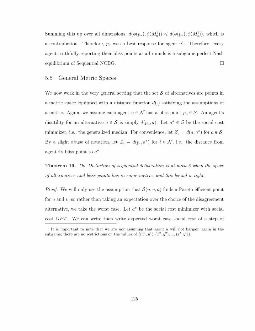
Summing this up over all dimensions, dpφppuq, φpMtuqq ď dpφppuq, φpM
tzqq, which is
a contradiction. Therefore, pu was a best response for agent u1. Therefore, every
agent truthfully reporting their bliss points at all rounds is a subgame perfect Nash
equilibrium of Sequential NCBG.
5.5 General Metric Spaces
We now work in the very general setting that the set S of alternatives are points in
a metric space equipped with a distance function dp¨q satisfying the assumptions of
a metric. Again, we assume each agent u P N has a bliss point pu P S. An agent’s
disutility for an alternative a P S is simply dppu, aq. Let a˚ P S be the social cost
minimizer, i.e., the generalized median. For convenience, let Za “ dpa, a˚q for a P S.
By a slight abuse of notation, let Zi “ dppi, a˚q for i P N , i.e., the distance from
agent i’s bliss point to a˚.
Theorem 19. The Distortion of sequential deliberation is at most 3 when the space
of alternatives and bliss points lies in some metric, and this bound is tight.
Proof. We will only use the assumption that Bpu, v, aq finds a Pareto efficient point
for u and v, so rather than taking an expectation over the choice of the disagreement
alternative, we take the worst case. Let a˚ be the social cost minimizer with social
cost OPT . We can write then write expected worst case social cost of a step of
1 It is important to note that we are not assuming that agent u will not bargain again in thesubgame; there are no restrictions on the values of tpx1, y1q, px2, y2q, ..., pxt, ytqu.
125
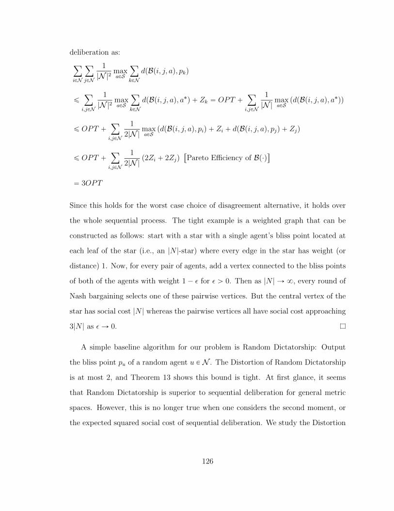
deliberation as:
ÿ
iPN
ÿ
jPN
1
|N |2maxaPS
ÿ
kPNdpBpi, j, aq, pkq
ďÿ
i,jPN
1
|N |2maxaPS
ÿ
kPNdpBpi, j, aq, a˚q ` Zk “ OPT `
ÿ
i,jPN
1
|N |maxaPS
pdpBpi, j, aq, a˚qq
ď OPT `ÿ
i,jPN
1
2|N |maxaPS
pdpBpi, j, aq, piq ` Zi ` dpBpi, j, aq, pjq ` Zjq
ď OPT `ÿ
i,jPN
1
2|N |p2Zi ` 2Zjq
“
Pareto Efficiency of Bp¨q‰
“ 3OPT
Since this holds for the worst case choice of disagreement alternative, it holds over
the whole sequential process. The tight example is a weighted graph that can be
constructed as follows: start with a star with a single agent’s bliss point located at
each leaf of the star (i.e., an |N |-star) where every edge in the star has weight (or
distance) 1. Now, for every pair of agents, add a vertex connected to the bliss points
of both of the agents with weight 1´ ε for ε ą 0. Then as |N | Ñ 8, every round of
Nash bargaining selects one of these pairwise vertices. But the central vertex of the
star has social cost |N | whereas the pairwise vertices all have social cost approaching
3|N | as εÑ 0.
A simple baseline algorithm for our problem is Random Dictatorship: Output
the bliss point pu of a random agent u P N . The Distortion of Random Dictatorship
is at most 2, and Theorem 13 shows this bound is tight. At first glance, it seems
that Random Dictatorship is superior to sequential deliberation for general metric
spaces. However, this is no longer true when one considers the second moment, or
the expected squared social cost of sequential deliberation. We study the Distortion
126
on this metric. define:
Squared-Distortion “ErpSCpaqq2spSCpa˚qq2
where the expectation is over the set of outcomes a produced by Sequential Deliber-
ation.
It is easy to see that Random Dictatorship has an unbounded Squared-Distortion.
Consider the simple graph with two nodes, a fraction f of the agents on one node and
1´ f on the other. Let f ă 12. Then the expected squared social cost of Random
Dictatorship is just fp1´ fq2 ` p1´ fqf 2 whereas the optimal solution has squared
social cost f 2, so Random Dictatorship has Squared-Distortion p1´ fq2f ` p1´ fq,
which is unbounded as f Ñ 0.
On the other hand, we show that Sequential deliberation has constant Squared-
Distortion even for general metric spaces. One way to interpret this result is that the
deviation of the social cost around its mean falls off quadratically instead of linearly,
which means the outcome of sequential deliberation is well-concentrated around its
mean value2. We will need the following technical lemma to characterize the outcome
of a round of bargaining.
Lemma 16. For all i, j, u P N and a P S we have that
dpBpi, j, aq, puq ď Zu ` 2 min pZi, Zjq `min pZa,max pZi, Zjqq
Proof. Assume w.l.o.g. that Zi ď Zj. Then the lemma statement reduces to
dpBpi, j, aq, puq ď Zu ` 2Zi `min pZa, Zjq (5.4)
Recall that Nash bargaining asserts that given a disagreement alternative a, agents
i and j choose that alternative o P S that maximizes:
Nash product “ pdppi, aq ´ dppi, oqq ˆ pdppj, aq ´ dppj, oqq
2 See also recent work by [140] that considers minimizing the variance of randomized truthfulmechanisms.
127

Maximizing this on a general metric yields that dpBpi, j, aq will be chosen on the pi
to pj shortest path (that is, the Pareto efficient frontier) at a distance ofdppi,pjq
2`
dppi,aq´dppj ,aq
2from pi. Therefore, we have that:
dpBpi, j, aq, piq “dppi, pjq
2`dppi, aq ´ dppj, aq
2(5.5)
Now we can show equation 5.4 by repeatedly using the triangle inequality. We have
dpBpi, j, aq, puq
ď dppi, puq ` dpBpi, j, aq, piq
“ dppi, puq `dppi, pjq
2`dppi, aq ´ dppj, aq
2
“
equation 5.5‰
ď dppi, a˚q ` dppu, a
˚q `
dppi, a˚q ` dppj, a
˚q ` dppi, a˚q ` dpa, a˚q
2´dppj, aq
2
“ Zu ` 2Zi `Zj ` Za ´ dppj, aq
2
Note that we can apply the triangle inequality again to get two bounds, since Zj ď
dppj, aq ` Za and Za ď dppj, aq ` Zj. Since both bounds must hold, we have that
dpBpi, j, aq, puq ď Zu ` 2Zi `min pZa, Zjq.
Now we can bound the Squared-Distortion of sequential deliberation.
Theorem 20. The Squared-Distortion of sequential deliberation for is at most 41
when the space of alternatives and bliss points lies in some metric.
Let OPT be the squared social cost of a˚. Note that OPT does not depend on
T . In particular, OPT “ př
iPN Ziq2“ř
i,jPN ZiZj.
Let ALG be the expected squared social cost of sequential deliberation with
T steps, where the disagreement alternative a P S is used in the final round of
bargaining. i and j are the last two agents to bargain, and pk is the bliss point of an
128

arbitrary agent. Using Lemma 16 we can write ALG as
ALG “ÿ
iPN
ÿ
jPN
1
|N |2
˜
ÿ
kPNdpBpi, j, aq, pkq
¸2
ď1
|N |2ÿ
i,jPN
˜
ÿ
kPNZk ` 2 min pZi, Zjq `min pZa,max pZi, Zjqq
¸2
“1
|N |2ÿ
i,jPN
˜
2|N |min pZi, Zjq ` |N |min pZa,max pZi, Zjqq `
˜
ÿ
kPNZk
¸¸2
Now we expand the square and analyze term by term, using the facts that
min px, yq2 ď xˆ y and max px, yq ď x` y.
“1
|N |2ÿ
i,jPN
˜
4|N |2 min pZi, Zjq2` |N |2 min pZa,max pZi, Zjqq
2`
˜
ÿ
kPNZk
¸2
` 4|N |2 min pZi, Zjqmin pZa,max pZi, Zjqq ` 4|N |min pZi, Zjq
˜
ÿ
kPNZk
¸
` 2|N |min pZa,max pZi, Zjqq
˜
ÿ
kPNZk
¸¸
ď1
|N |2ÿ
i,jPN
˜
4|N |2ZiZj ` |N |2 min pZa,max pZi, Zjqq2`OPT
` 4|N |2ZiZa ` 4|N |Zi
˜
ÿ
kPNZk
¸
` 2|N |Za
˜
ÿ
kPNZk
¸¸
We can trivially sum out the terms not involving a, leaving us with inequality 5.6.
ALG ď 9OPT `ÿ
i,jPN
˜
ZapZi ` Zjq ` 4ZiZa `2
|N |Za
˜
ÿ
kPNZk
¸¸
(5.6)
Note that the triangle inequality implies that for any i P N , Za ď dpa, piq ` Zi.
129

Applying this repeatedly in inequality 5.6 and simplifying yields:
ALG ď 9OPT `ÿ
i,jPN
˜
6ZiZj ` 5dpa, pjqZi ` dpa, piqZj `2
|N |pdpa, piq ` Ziq
˜
ÿ
kPNZk
¸¸
“ 17OPT `ÿ
iPN
˜
2dpa, piq
˜
ÿ
kPNZk
¸
`ÿ
jPN5dpa, pjqZi ` dpa, piqZj
¸
Recall that Theorem 19 implies thatř
iPN dpa, piq ď 3ř
iPN Zi.
ALG ď 17OPT ` 6OPT ` 15OPT ` 3OPT “ 41OPT
5.6 Conclusion and Open Directions
In this chapter, we took a first step to developing a theory around practical delibera-
tion schemes. We employed the implicit utilitarian model to evaluate the properties
of our deliberation mechanism for approximating the utilitarian optimum under lim-
ited information. We defined a general protocol for deliberation, and demonstrated
a host of strong and desirable properties under the assumption that the space of
possible outcomes form a median graph, along with more general guarantees when
the space of possible outcomes are merely constrained to be metric.
We suggest several future directions. First, we do not have a general charac-
terization of the Distortion of sequential deliberation for metric spaces. We have
shown that for general metric spaces there is a small but pessimistic bound on the
Distortion of 3, but that for specific metric spaces the Distortion may be much lower.
We do not have a complete characterization of what separates these good and bad
regimes.
More broadly, an interesting question is extending our work to take opinion
dynamics into account, i.e., proving stronger guarantees if we assume that when
two agents deliberate, each agent’s opinion moves slightly towards the other agent’s
opinion and the outside alternative. Furthermore, though we have shown that all
130

agents deliberating at the same time does not improve on dictatorship, it is not clear
how to extend our results to more than two agents negotiating at the same time.
This runs into the challenges in understanding and modeling multiplayer bargain-
ing [90, 110, 26].
131

6
Metric Implicit Utilitarian Voting with ConstantSample Complexity
In the previous chapter, we explored a novel connection between the cooperative
game theoretic solution concept of Nash bargaining and social choice protocols in
a metric implicit utilitarian model. However, Nash bargaining itself requires agents
to reason over their cardinal preferences or utilities. In this chapter, we continue
investigating social choice in the metric implicit utilitarian model by defining purely
ordinal mechanisms, in the sense that they require neither communication of nor
reasoning over cardinal preferences. We focus on designing practical and lightweight
mechanisms that use at most a constant number of simple ordinal queries to provide
guarantees with respect to Distortion and Squared Distortion.
Acknowledgements. These results are published [64], and are joint work with Ashish
Goel, Kamesh Munagala, and Nina Prabhu.
132

6.1 Introduction
Consider the social choice problem of deciding on an allocation of public tax dollars to
public projects. This is a voting problem over budgets. Clearly, the number of voters
in such situations can be large. More interestingly, unlike in traditional social choice
theory, there is no reason to believe that the number of alternatives (budgets) is small.
It is therefore unreasonable to assume that we can elicit full ordinal preferences over
alternatives from every agent. For a voting mechanism to be practical in such a
setting, one would ideally like it to require only an absolute constant number of
simple queries, regardless of the number of voters and alternatives. We call this
property constant sample complexity, and we explore mechanisms of this sort in this
chapter.
We define our model more formally in Section 6.1.3, but at a high level, we have
a set N of agents (or voters) and a set of alternatives S, from which we must choose
a single outcome. We assume that N and S are both large, and that eliciting the
full ordinal rankings may be prohibitively difficult. Instead, we work with an ordinal
query model, and a constant sample complexity mechanism uses only a constant
number of these queries.
• Top-k Query. “What are your k favorite alternatives, in order?” (We call a
top-1 query a favorite query); and
• Comparison Query. “Which of two given alternatives do you prefer?”
Query models are not just of theoretical interest. They can be used to reduce
cognitive overload in voting. For example, in the context of Participatory Budget-
ing [1], the space of possible budget allocations is large, and one mechanism is to ask
voters to compare two proposed budgets. Similarly, in a context like transportation
policy for a city, a single alternative can be an entire transportation plan. In such
133

examples, not only are there many alternatives, but it may be infeasible to expect
voters to compare more than two alternatives at the same time. We stress that con-
stant sample complexity is particularly important in settings where there may be a
large number of possibly complex alternatives.
To evaluate the quality of our mechanisms, we adopt the implicit utilitarian
perspective with metric constraints [31, 46, 8, 79, 7, 67]. That is, we assume that
agents have cardinal costs over alternatives, and these costs are constrained to be
metric, but asking agents to work with or report cardinal costs is impractical or
impossible. We want to design social choice mechanisms to minimize the total social
cost, but our mechanism is constrained only to use ordinal queries, that is, those
that can be answered given a total order over alternatives. We therefore measure
the efficiency of a mechanism as its Distortion (see Section 6.1.3), the worst case
approximation to the total social cost.
6.1.1 Results
The starting point for our inquiry is the constant sample complexity Random Dicta-
torship mechanism. The algorithm asks a single favorite query from an agent chosen
uniformly at random, and has a tight Distortion bound of 3 [8]. In this chapter, we
provide two new mechanisms (Random Referee and Random Oligarchy) that improve
on this simple baseline in three different ways, outlined in each of our three technical
sections. We hope that our work inspires future research on similarly lightweight
mechanisms for social choice in large decision spaces.
Random Referee: Comparison Queries and Squared Distortion. In Section 6.2, we show
that one disadvantage of Random Dictatorship lies not in its Distortion, but in
its variance. For randomized mechanisms, Distortion is measured as the expected
approximation to the first moment of social cost. However, in many social choice
134

problems, we might want a bound on the risk associated with a given mechanism. We
capture this via Squared Distortion, as suggested in [65]. The Squared Distortion (see
Definition 17 in Section 6.1.3) is the expected approximation to the second moment
of social cost. A mechanism with constant Squared Distortion has both constant
Distortion and constant coefficient of variation of the Distortion.
We show that mechanisms using only top-k queries (including Random Dicta-
torship) have Squared Distortion Ωp|S|q. This motivates us to expand our query
model to incorporate information about the relative preferences of agents between
alternatives, i.e. use comparison queries. We define a novel mechanism called Ran-
dom Referee (RR) that uses a random voter as a referee to compare the favorite
alternatives of two other random voters (see Definition 18 in Section 6.2). Our main
result in Section 6.2 is Theorem 22: The Squared Distortion of RR is at most 21.
This also immediately implies that the Distortion of RR is at most 4.583.
Random Referee: Euclidean Plane. In Section 6.3, we show that top-k only mecha-
nisms (again, including Random Dictatorship) achieve their worst case Distortion
even on benign metrics such as low dimensional Euclidean spaces. We analyze a spe-
cial case on the Euclidean plane and prove that the Distortion of Random Referee
beats that of any top-k only mechanism. While the improvement we prove in Sec-
tion 6.2 is quantitatively small, it is qualitatively interesting: we demonstrate that
by using a single comparison query, Random Referee can exploit the structure of the
metric space to improve Distortion, whereas Random Dictatorship or any other top-
k only mechanism cannot. We conjecture this result extends to Euclidean spaces in
any dimension, and present some evidence to support this conjecture in Section 6.5.
Random Oligarchy: Favorite Only Mechanisms. In Section 6.4, we consider mech-
anisms that are restricted to favorite queries and show that constant complexity
135

mechanisms are nearly optimal. We present a mechanism that uses only three fa-
vorite queries that has Distortion at most 3 for arbitrary |S|; however, it also has
Distortion for small |S| that improves upon the best known favorite only mecha-
nism from [85] that uses at most minp|N | ` 1, |S| ` 1q favorite queries. Comparing
with a lower bound for favorite only mechanisms, Random Oligarchy has nearly op-
timal distortion and constant sample complexity. Though this mechanism does not
have constant Squared Distortion like Random Referee, we present it to demonstrate
again the surprising power of constant sample complexity randomized social choice
mechanisms in general, and of queries to just three voters in particular.
Techniques. We use different techniques to prove our different positive results. The
proof of Squared Distortion (Theorem 22 in Section 6.2) relies heavily on Lemma 17,
in which we prove (essentially) that Random Referee chooses a low social cost al-
ternative as long as at least two of the three agents chosen at random are near the
social optimum.
The proof of Distortion for Euclidean spaces (Theorem 25 in Section 6.3) is the
most technical result. We show that we can upper bound the Distortion of a mech-
anism by the worst case “pessimistic distortion,” of just a constant size tuple of
points, where the “pessimistic distortion” considers all permutations of the points as
participating in Random Referee and allows OPT to choose the optimal point on just
this tuple. This allows us to employ a computer assisted analysis by arguing that if a
high Distortion instance exists, we can detect it as an instance with a small constant
number of points on a sufficiently fine (but finite) grid in the Euclidean plane. This
approach may be of independent interest for providing tighter Distortion bounds for
mechanisms in specific structured metric spaces.
136

6.1.2 Related Work
Distortion of Randomized Social Choice Mechanisms in Metrics. The Distortion of ran-
domized social choice mechanisms in metrics has been studied in [31, 8, 79, 85].
Of particular interest to us are the Random Dictatorship mechanism that uses
a single favorite query and the 2-Agree mechanism [85] that uses at most most
minp|N | ` 1, |S| ` 1q favorite queries. Random Dictatorship has an upper bound on
Distortion of 3 [8], and 2-Agree provides a strong guarantee on Distortion when |S|
is small (better than Random Dictatorship for |S| ď 6). There is ongoing work on
analyzing the Distortion of randomized ordinal mechanisms for other classic opti-
mization problems like graph optimization [2] and facility location [9].
Squared Distortion and Variance. We are aware of two papers in mechanism design
that consider the variance of mechanisms for facility location on the real line [140] and
kidney exchange [62]. Our work is more related to the former, but is not restricted to
the real line, and does not focus on characterizing the tradeoff between welfare and
variance. Using Squared Distortion as a proxy for risk was introduced in [65] along
with the sequential deliberation protocol. Unlike sequential deliberation, Random
Referee makes a constant number of ordinal queries. The most important baseline
for Squared Distortion is the deterministic Copeland rule, which has Distortion 5 [7]
and therefore Squared Distortion 25. However, Copeland requires the communi-
cation of Ωp|N ||S| logp|S|qq bits [55], essentially the entire preference profile. Our
Random Referee mechanism has constant sample complexity, and has better bounds
on Squared Distortion (21) and Distortion (4.583) than the Copeland mechanism.
Communication Complexity. For a survey on the complexity of eliciting ordinal pref-
erences to implement social choice rules, we refer the interested reader to [34]. Of
particular interest to us is [55], in which the authors comprehensively characterize
137
the communication complexity (in terms of the number of bits communicated) of
common deterministic voting rules. A favorite query requires Oplogp|S|qq bits of
communication, so our mechanisms have constant sample complexity, but logarith-
mic communication complexity. [32] and [42] design social choice mechanisms with
low communication complexity when there are a small number of voters, but poten-
tially a large number of alternatives. All of our mechanisms have guarantees that
are independent of the number of voters.
Strategic Incentives. We do not consider truthfulness chapter, and we do not use the
term mechanism to imply any such property. While strategic incentives are not the
focus of this work, we note that any truthful mechanism must have Distortion at least
3 [67]. Random Dictatorship has a Distortion of 3, and is therefore in some sense
optimal among exactly truthful mechanisms. Other works suggest that truthfulness
is also incompatible with the weaker notion of Pareto efficiency in randomized social
choice [33, 15]. Still other authors have considered the problem of truthful welfare
maximization under range voting [69] and threshold voting [27].
6.1.3 Preliminaries
We have a set N of agents (or voters) and a set S of alternatives, from which we
must choose a single outcome. For each agent u P N and alternative a P S, there is
some underlying dis-utility dupaq. Let pu “ argminaPSdupaq, that is, pu is the most
preferred alternative for agent u. Ordinal preferences are specified by a total order
σu consistent with these dis-utilities (i.e., an alternative is ranked above another only
if it has lower dis-utility). A preference profile σpNq specifies the ordinal preferences
of all agents. A deterministic social choice rule is a function f that maps a preference
profile σpNq to an alternative a P S. A randomized social choice rule maps a preference
profile σpNq to a distribution over S.
138

We consider mechanisms that implement a randomized social choice rule using a
constant number of queries of two types. A top-k query asks an agent u P N for the
first k preferred alternatives according to the order σu (ties can be broken arbitrarily).
We refer to a top-1 query as a favorite query, that asks an agent u P N for her most
preferred alternative pu. A top-k only mechanism f uses only top-k queries, for
some constant k (constant with respect to |N | and |S|). Most of our lower bounds
or impossibilities will be for any top-k only mechanism (for constant k), whereas our
positive results will only need favorite and comparison queries. A comparison query
with alternatives a P S and b P S asks an agent u P N for argminxPta,budupxq.
We use the term mechanism to clarify that our algorithms are in a query model.
However, it is important to note that mechanisms so defined are still randomized
social choice rules in the formal sense as long as they do not make queries based on
exogenous information (e.g., names of participants). Our mechanisms will in fact
be randomized social choice rules, and thus can be appropriately compared to other
such rules in the literature that do not explicitly use a query model. By using the
term mechanism, we do not mean to imply any strategic properties.
Distortion and Sample Complexity. We measure the quality of an alternative a P S by
its social cost, given by SCpaq “ř
uPN dupaq. Let a˚ P S be the minimizer of social
cost. We define the commonly studied approximation factor called Distortion [142],
which measures the worst case approximation to the optimal social cost of a given
mechanism. We use the expected social cost if a is the outcome of a randomized
mechanism, and we seek to minimize Distortion.
Definition 16. The Distortion of an alternative a is Distortionpaq “ SCpaqSCpa˚q
. The
Distortion of a social choice mechanism f is
Distortionpfq “ suptdupaqu
EfpσpNqqDistortionpaq
139

where σpNq is a preference profile consistent with tdupaqu.
We assume that S is a set of points in a metric space such that dis-utility can
be measured by the distance from an agent. Specifically, we assume there is a
distance function d : pNYSqˆpNYSq Ñ Rě0 satisfying the triangle inequality such
that dupaq “ dpu, aq. The metric assumption is common in the implicit utilitarian
literature [8, 79, 65, 85, 46, 7, 67]. It is also a natural assumption for capturing social
choice problems for which there is a natural notion of distance between alternatives.
For example, in our original motivating example of public budgets, there is are
natural notions of distance between alternatives in terms of dollars.
We do not assume access to σpNq directly, which may be prohibitively difficult to
elicit when there are many alternatives. Instead, we work with a query model. The
queries are ordinal in the sense that they can be answered given only the information
in σpNq. A mechanism f has constant sample complexity if there is an absolute
constant c such that for all S, N , and σpNq, f can be implemented using at most
c queries. In this chapter, we consider top-k (and the special case of favorite) and
comparison queries, and explore mechanisms with constant sample complexity.
Squared Distortion. It is easy to see that randomization is necessary for constant
sample complexity mechanisms to achieve constant Distortion. AsN grows large, any
deterministic mechanism with constant sample complexity deterministically ignores
(asks no queries of and receives no information from) an arbitrarily large fraction of
N . An adversary can therefore place an alternative with 0 dis-utility for arbitrarily
many agents; this gives a lower bound for Distortion approaching N as N becomes
large.
This naturally leads us to ask: If we look at the distribution of outcomes produced
by the mechanism, is this distribution well behaved? Following [65], we capture this
notion via Squared Distortion: essentially the approximation to the optimal second
140

moment of social cost.
Definition 17. The Squared Distortion of an alternative a P S is Distortion2paq “
´
SCpaqSCpa˚q
¯2
. The Distortion of a social choice mechanism f is
Distortion2pfq “ sup
tdupaqu
EfpσpNqqDistortion2paq
where σpNq is a preference profile consistent with tdupaqu.
Note that a mechanism with constant Squared Distortion has both constant Dis-
tortion (by Jensen’s inequality), and constant coefficient of variation. One way to
interpret having constant Squared Distortion is that the deviation of the social cost
around its mean falls off quadratically instead of linearly, which means that the so-
cial cost of such a mechanism is well concentrated around its mean value. We note
that this interpretation gives randomized social choice mechanisms with constant
Squared Distortion an interesting application in candidate selection. In particular,
one can imagine running such a mechanism (like our Random Referee) to generate a
candidate list on which one can use a deterministic (but potentially complex) voting
mechanism like Copeland.
A related approach to understanding the distributional properties of a randomized
mechanism is to characterize the tradeoff between Distortion (approximation to the
first moment) and the variance of randomized mechanisms [140]. Our specific goal
in this chapter is to develop a mechanism that achieves constant Distortion and
constant variance, and this combination is captured by having constant Squared
Distortion. We leave characterizing the exact tradeoff between the quantities as an
interesting open direction.
141
6.2 Random Referee and Squared Distortion
Our first result is Theorem 21: Mechanisms that only elicit top-k preferences, for
constant k, must necessarily have Squared Distortion that grows linearly in the size
of the instance. This holds even for mechanisms that elicit the top-k preferences of
all of the voters, mechanisms which would not have constant sample complexity.
Theorem 21. Any top-k only social choice mechanism has Squared Distortion Ωp|S|q.
Proof. We want to construct a single ordinal profile over top-k preferences such that
for all randomized social choice mechanisms, there is some instantiation of these
top-k preferences in a metric space on which the mechanism has Squared Distortion
Ωp|S|q. The top-k ordinal profile is simple: Each agent u P N has completely unique
top-k preferred feasible alternatives Su Ď S. There are no other alternatives, so
|S| “ k|N | “ Θp|N |q (note that a top-k only mechanism must have constant k).
Any randomized social choice mechanism must choose a distribution on S, so in
particular, there will be some u˚ P N such that the mechanism puts at least 1|N |
probability mass on the top-k preferred alternatives of u˚. Given this, consider a
metric space, consistent with the top-k preference profile, where S˚u forms a small
clique well separated from all of the other alternatives which form a large clique.
More formally, let 0 ă ε ď 1|N |. All pairwise distances are ε except those between
the small and large clique. Instead, dpu, aq “ 1 for all u ‰ u˚, a P Su˚ , and similarly
dpu˚, aq “ 1 for all a P SzSu˚ .
Then the Squared social cost of choosing a P Su˚ is simply p|N |´1q2, whereas the
optimal solution chooses any a P SzSu˚ for Squared social cost of p1` εp|N | ´ 1qq2 ď
p1` ε|N |q2. Since the mechanism chooses a P Su˚ with probability at least 1|N |, we
142

can lower bound the Squared Distortion of any top-k only mechanism f as follows.
Distortion2pfq ě
1
|N |
p|N | ´ 1q2
p1` ε|N |q2
ěp|N | ´ 1q2
4|N |“ Ωp|S|q
The problem with top-k only mechanisms, exploited in the proof of Theorem 21,
is that they treat agents as indifferent between their pk`1qst favorite alternative and
their least favorite alternative. This motivates the expansion of our query model to
include comparison queries. Recall that a comparison query with alternatives a P S
and b P S asks an agent u P N for argminxPta,budupxq. We use a single comparison
query in our Random Referee mechanism.
Definition 18. The Random Referee (RR) mechanism samples three agents u, v, w P
N independently and uniformly at random with replacement. u and v are asked for
their favorite feasible alternatives pu and pv in S, and then w is asked to compare pu
and pv. Output whichever of the two alternatives w prefers.
Upper Bound for Random Referee. Our main result in this section is Theorem 22:
The Squared Distortion of RR is at most 21. This also implies that the Distortion
of RR is at most 4.583. As far as we are aware, no randomized mechanism has lower
Squared Distortion in general.
We will need the following technical lemma. Let a˚ P S be the social cost min-
imizer. The basic intuition behind Random Referee is that it will choose a low
social cost alternative as long as any two out of the three agents selected are near
the optimal alternative a˚. Lemma 17 makes this intuition formal. For conve-
nience, let Zu “ dpu, a˚q for u P N , i.e., the dis-utility of a˚ for agent u. Let
143

Cptu, vu, wq “ argminyPtpu,pvudpw, yq, that is, the alternative Random Referee out-
puts when u and v are selected to propose alternatives and w chooses between them.
Lemma 17. For all u, v, w, x P N ,
dpCptu, vu, wq, xq ď Zx ` 2 min
#
maxpZu, Zvq,
Zw `minpZu, Zvq.
Proof. One should think of u, v P N as the agents drawn to present their favorite
alternative, w as the referee, and x as the agent from whom we measure the dis-utility
of the resulting outcome. The triangle inequality implies that
dpCptu, vu, wq, xq ď Zx ` dpa˚, Cptu, vu, wqq.
We give two separate upper bounds on dpa˚, Cptu, vu, wqq, thus yielding the min. We
will frequently use the fact that for all u P N , dpu, a˚q ď dppu, uq ` dpu, a˚q ď 2Zu.
This follows from the the definition of pu: the favorite alternative of u, and thus no
greater in distance from u than a˚. The first bound is straightforward: Cptu, vu, wq P
tpu, pvu by definition of Random Referee, so
dpa˚, Cptu, vu, wqq ď max pdpa˚, puq, dpa˚, pvqq
ď 2 max pZu, Zvq
In a sense, this bound concerns the situation where both u and v are near a˚, but
w is far away from a˚. Now we argue for the second bound. Suppose without
loss of generality that Zu ď Zv. w chooses either pu or pv. If w chooses pu, then
dpa˚, Cptu, vu, wqq “ dpa˚, puq ď 2dpa˚, uq “ 2 minpZu, Zvq, and so the bound holds.
144

If w chooses pv, then dpw, pvq ď dpw, puq, which implies
dpa˚, Cptu, vu, wqq “ dpa˚, pvq
ď dpa˚, wq ` dpw, puq
ď Zw ` dpw, a˚q ` dpa˚, puq
ď 2Zw ` 2Zu
“ 2 pZw `minpZu, Zvqq
and again the bound holds. In either case, dpa˚, Cptu, vu, wqq is at most 2 pZw `minpZu, Zvqq.
Intuitively, this bound concerns the situation where w and u are close to a˚, but v
is far away from a˚. Taking the better of this bound with the dpa˚, Cptu, vu, wqq ď
2 maxpZu, Zvq bound through the min and factoring out the 2 yields the lemma.
Using Lemma 17, we can upper bound the Squared Distortion of Random Referee
by 21. This is in contrast to the Ωp|S|q Squared Distortion of any favorite only
mechanism (see Theorem 21).
Theorem 22. The Squared Distortion of Random Referee is at most 21.
Proof. Let OPT be the optimal squared social cost, that is, the squared social cost
of a˚, where a˚ P S is the social cost minimizer. Recall that Zu “ dpu, a˚q. Then
OPT “
˜
ÿ
uPN
Zu
¸2
“ÿ
uPN
ÿ
vPN
ZuZv.
Let ALG be the expected squared social cost of Random Referee. The expectation
can be written out as
ALG “1
|N |3
ÿ
u,v,wPN
˜
ÿ
xPN
dpCptu, vu, wq, xq
¸2
.
145

Let α “ min pmaxpZu, Zvq, Zw `minpZu, Zvqq . We apply Lemma 17 and simplify.
ALG ď1
|N |3
ÿ
u,v,wPN
˜
ÿ
xPN
pZx ` 2αq
¸2
Noting that α does not depend on x, we can expand the square and simplify to find
ALG ď OPT `4
|N |3
ÿ
u,v,wPN
˜
α2|N |2 ` α|N |
ÿ
xPN
Zx
¸
.
Now we sum each term separately. Let
T1 “4
|N |3
ÿ
u,v,wPN
α2|N |2
T2 “4
|N |3
ÿ
u,v,wPN
α|N |ÿ
xPN
Zx
We will use the following basic facts: for any real numbers a, b ě 0, pminpa, bqq2 ď a¨b,
maxpa, bq ď a` b, and minpa, bq ¨maxpa, bq “ a ¨ b.
T1 ď4
|N |
ÿ
u,v,wPN
pmaxpZu, Zvq pZw `minpZu, Zvqq
ď4
|N |
ÿ
u,v,wPN
ppZu ` ZvqZw ` ZuZvq
“ 12OPT
Similarly, we analyze the second term using the fact that α ď Zu ` Zv.
T2 “4
|N |3
ÿ
u,v,wPN
α|N |ÿ
xPN
Zx
ď4
|N |2
ÿ
u,v,wPN
pZu ` Zvqÿ
xPN
Zx
“ 8OPT
Adding together all of the terms, ALG ď 21OPT .
146

This immediately yields the root mean square Distortion bound via Jensen’s
inequality.
Corollary 5. The Distortion of Random Referee is at most?
21 « 4.583.
6.3 Distortion of Random Referee on the Euclidean Plane
Though the upper bound on the Distortion of Random Referee is slightly worse than
that of Random Dictatorship, we now show another advantage of using a comparison
query: Such mechanisms can exploit structure in specific metric spaces that favorite-
only mechanisms cannot. In other words, we show that the Distortion of Random
Referee improves significantly for more structured metric spaces, while top-k only
mechanisms do not share this property.
We examine the Distortion of Random Referee on a specific canonical metric
of interest: the Euclidean plane when dpu, puq “ 0 for every u P N . The second
assumption, functionally equivalent to assuming N Ď S, simplifies our analysis con-
siderably, and corresponds to the 0-decisive case in [8, 85]. We note that in examples
where |S| is very large, the assumption becomes more innocuous. If we consider
our opening example of public budgets, the assumption is something like this: every
agent is allowed to propose their absolute favorite over all budgets, and we assume
that this budget pu has dis-utility of 0. We consider the Euclidean plane because the
problem of minimizing distortion on the real line can be solved exactly [8], whereas
we are unaware of any results for the Euclidean plane that are stronger than those
for general metric spaces.
6.3.1 Lower Bounds for Distortion in the Restricted Model.
We begin by giving lower bounds to demonstrate that our simplifying assumptions
still result in a nontrivial problem in two senses: (1) the Distortion of randomized
social choice mechanisms are still bounded away from 1 and (2) any top-k only
147

mechanism (one that elicits the top k preferred alternatives of agents) for constant
k has Distortion at least 2 as |N | and |S| become large.
Theorem 23. The Distortion of a randomized social choice mechanism is at least
1.2 generally, and at least 1.118 for the Euclidean plane, even when dpu, puq “ 0 for
every u P N .
Figure 6.1: Example for Theorem 23. The red squares are agents as well asalternatives.
Proof. We begin with the more general claim. Consider a star graph with three
leaves and three agents, one agent at each leaf, as depicted in Figure 6.1. All four
points are also alternatives, and the distance between an agent and the colocated
alternative is 0. Call the central vertex B and the set of outer vertices R. We want to
construct a single ordinal preference profile such that for all randomized social choice
mechanisms, there is some metric space that induces this preference profile and for
which the mechanism has Distortion at least 1.2. The preference profile is simple:
each of the three agents prefer their colocated alternative to the central alternative
to either of the other leaf alternatives. We induce this profile via two metric spaces.
In both spaces, @v P R, dpv,Bq “ 1 (that is, the solid lines in Figure 6.1); the spaces
will differ in the distances between points inside of R (that is, the dashed lines in
Figure 6.1).
First, suppose that @v, v1 P R, v ‰ v1, dpv, v1q “ 2. Then the social cost of B is
3, and the social cost of every vertex in R is 4; clearly the distortion of B is 1 and the
distortion of v P R is 43. Let PrpRq be the probability that a randomized ordinal
148

social mechanism chooses some v P R, and let PrpBq be the probability that the
same mechanism chooses B. Then on this metric, the Distortion of the mechanism
is (in expectation) just PrpBq ` p43qPrpRq.
Second, suppose that @v, v1 P R, v ‰ v1, dpv, v1q “ 1 ` ε for some ε P p0, 0.5q.
Then the social cost of B is 3, and the social cost of every alternative in R is 2p1`εq,
so the distortion of B is 32p1`εq
and the distortion of v P R is 1. Then on this metric,
the Distortion of the mechanism is (in expectation) 32p1`εq
PrpBq ` PrpRq.
A social choice mechanism with only ordinal information cannot distinguish the
cases, and must set some values for PrpRq and PrpBq that sum to 1, so such a
mechanism cannot have Distortion less than
max
ˆ
PrpBq `4
3PrpRq,
3
2p1` εqPrpBq ` PrpRq
˙
.
This expression is minimized by setting PrpRq to 2`2ε5´4ε
(and PrpBq “ 1 ´ PrpRq)
yielding a Distortion of
4
3´
ˆ
1
3
˙ˆ
2` 2ε
5´ 4ε
˙
ÝÑ 65 as εÑ 0
The argument for the lower bound of 1.118 on the Euclidean plane is similar.
Now, the first case places the three points in R on a unit circle around the central
point B, equidistant from one another. The law of cosines implies that @v, v1 P
R, v ‰ v1, dpv, v1q “a
2´ 2 cosp120˝q « 1.732. In the second case, the angular
distance between consecutive points in R is 60˝, so that two pairwise distances are
1, and one pairwise distance isa
2´ 2 cosp120˝q. Completing the same argument as
before yields the bound of 1.11.
Theorem 24. The Distortion of any top-k only mechanism goes to 2 as |S| and |N |
become large, even on the Euclidean plane when dpu, puq “ 0 for every u P N .
149

Proof. The construction for this lower bound follows that of Theorem 21. We briefly
consider the argument for completeness. There are |S|k agents, and for each agent
u, there are k unique alternatives Su Ă S that are ε distance away from them. Su
are the top-k preferred alternatives for u. There are no other alternatives. Consider
any top-k only mechanism (recall that k is constant). Such a mechanism chooses
a distribution over alternatives, and thus Du˚ P N with top-k preferred alternatives
Su˚ such that the mechanism puts at least 1|N | probability mass on Su˚ .
Suppose that the other |N | ´ 1 agents are arrayed in a circle such that the
pairwise distance of diameter δ (clearly, if ε is small enough, such an arrangement
need not violate our earlier construction). Further, suppose the distance from u˚ to
the center of this circle is 1. Then the social cost of any alternative in Su˚ is at least
p|N | ´ 1qp1 ´ ε ´ δ2q, and the social cost of any alternative not in Su˚ is at most
1` εδ2` p|N | ´ 2qpδ` 2εq. Therefore, the Distortion of choosing any alternative in
Su˚ is at least
p|N | ´ 1qp1´ ε´ δ2q
1` εδ2` p|N | ´ 2qpδ ` 2εq.
As ε and δ approach 0, the above approaches |N | ´ 1. The Distortion of choos-
ing any alternative not in Su˚ is clearly just 1. Since the mechanism chooses an
alternative in Su˚ with probability at least 1|N | (say 1|N | ` α, where α ě 0) and
an alternative not in Su˚ with the remaining 1 ´ 1|N | ´ α probability, the over
Distortion is lower bounded byˆ
1
|N |` α
˙
p|N | ´ 1q `
ˆ
|N | ´ 1
|N |´ α
˙
“ 2´ 2|N | ` α p|N | ´ 2q
ě 2´ 2|N |
Ñ 2 as |N | Ñ 8.
150

6.3.2 Upper Bound for Distortion of Random Referee in the Restricted Model.
Our positive result in this section demonstrates that a single comparison query is suf-
ficient to construct a mechanism (Random Referee) with Distortion bounded below
1.97 for arbitrary |S| and |N |. We note that the bound in the theorem seems very
slack; our goal is simply to show that using a comparison query provably decreases
Distortion. We conjecture the actual bound is below 1.75 based on computer assisted
search, but leave proving this stronger bound as an interesting open question.
Theorem 25. The worst case distortion of Random Referee is less than 1.97 when
dpu, puq “ 0 for every u P N , S Ď R2, and for x, y P R2 dpx, yq “ x´ y2.
In the remainder of this section, we sketch the proof of Theorem 25. Proofs of
some of the technical lemmas are in the appendix. Suppose for a contradiction that
there is a set N of agents in R2 such that the Distortion of Random Referee is at
least 1.97 under the Euclidean metric. We will successively refine this hypothesis
for a contradiction, finally arguing that it implies that some “bad” instance would
appear on an exhaustive computer assisted search over a finite grid.
The crucial lemmas bound the pessimistic distortion of any set of five points in
R2 and relate this to the actual distortion. The quantity is pessimistic because it
allows “OPT” to choose a separate point for every 5-tuple; the numerator of each
5-tuple is just a rewriting of the expected social cost of Random Referee. In this
section, since we assume dpu, puq “ 0, it will not be necessary to refer to u and pu
separately, and it will be convenient to let Cptpu, pvu, pwq “ argminaPtpu,pvudppw, aq.
Definition 19. The pessimistic distortion1 of P “ tx1, x2, x3, x4, x5u Ă R2 is defined
as
PDpPq :“SCRRavgpPqOPTavgpPq
1 Note that pessimistic distortion is technically a function of the mechanism used; we will use itexclusively in reference to Random Referee.
151
where SCRRavgpPq is the average social cost of Random Referee, which we can write
as
1
30
5ÿ
i“1
5ÿ
jąi
ÿ
k‰i,j
ÿ
l‰i,j,k
dpxl, Cptxi, xju, xkqq,
and the average cost of the optimal solution is
OPTavgpPq :“ minyPR2
1
5
5ÿ
r“1
dpxr, yq.
Finally, PDpPq “ 1 if x1 “ x2 “ x3 “ x4 “ x5.
The first lemma relates this pessimistic distortion to the actual Distortion of
Random Referee. The worst case (over 5-tuples) pessimistic distortion upper bounds
the Distortion of Random Referee. Interestingly, this statement is not specific to the
Euclidean plane, suggesting that our approach may be broadly applicable for proving
stronger Distortion bounds on other specific metrics of interest.
Lemma 18. If PDpP q ď β for all P “ tx1, . . . , x5u Ă R2 then the Distortion of
Random Referee is at most β on R2.
Proof. Observe that we can rewrite the Distortion of Random Referee as a summation
over all possible 5-tuples of points. Let P be a multiset of points (i.e., possibly with
repeats). Let ρpPq be an ordering of P . Let
CpρpPqq “ Cptρ1pPq, ρ2pPqu, ρ3pPqq.
We can rewrite the Distortion of Random Referee over permutations of 5-tuples as
1|N |4
ř
i,j,k,lPN dppl, Cptpi, pju, pkq1|N |
ř
iPN dppi, a˚q
“
ř
PĂPN PrpPq 15!
ř
ρpPqř
lPt4,5u dpρlpPq, CpρpPqqq1|N |
ř
iPN dppi, a˚q
.
152

In words, we are considering all 5-tuples (with replacement) of agent points, and for
each we consider the average distance over all orderings of the five agent points of
the distance between the last two points and the outcome of Random Referee when
the first three agents participate. This is in turn upper bounded by allowing OPT
to choose a different a˚ for every 5-tuple, so that the Distortion is at most
ÿ
PĂPN
PrpPq15!
ř
ρpPqř
lPt4,5u dpρlpPq, CpρpPqqqOPTavgpPq
ď maxPĂPN
PrpPq15!
ř
ρpPqř
lPt4,5u dpρlpPq, CpρpPqqqOPTavgpPq
.
To complete the proof, note that SCRRavgpPq is equal to the numerator. We
start with all 120 orderings of the 5 points and avoid double counting the symmetric
cases that arise from swapping the two points from which we take the argmin and
swapping the two points from which we measure distance.
Now we can refine our original hypothesis: without loss of generality, assume for
a contradiction that there is a multiset P “ tx1, . . . , x5u Ď R2 with PDpPq ě 1.97.
We argue that we can further refine our hypothesis by assuming a canonical form in
relation to a finite grid.
Lemma 19. Let G be a δ-fine grid: G “ t0, δ, 2δ, . . . , δ´1δ, 1u2 where δ ą 0 and
1δ P N. There is a set of points Q “ ty1, y2, y3, y4, y5u such that PDpQq “ PDpPq
and Q has the properties:
1. Q Ă r0, 1` δs2,
2. maxi,j dpyi, yjq “ 1,
3. and these two maximally separated points yi and yj have the forms yi “ pαδ, 0q, yj “
pαδ, 1q for some α P t0, 1, 2, . . . , 1δu
153

Proof. We note that the pessimistic distortion of P is invariant to scaling, rotation,
and translation of P . This follows because the pessimistic distortion is still defined
in terms of euclidean distances. Given this, the argument for the Lemma is simply
that we can construct Q by rotations, translations, and scaling.
First scale P so that the maximum distance separating two points is 1 (note that
at least two points are not equal). Next, rotate the points so that the line between
these maximally separated points is vertical. Finally, translate the points until these
maximally separated points have the appropriate forms - that is to say, until they
lie exactly at grid points, and all other points are within r0, 1` δs2. To see that this
is possible, note that since they are the maximally separated points, no other points
can lie outside r0, 1s in the vertical dimension. In the horizontal dimension, the total
width spanned by the other points is at most 1, and we may need to expand by as
much as δ in order to align the maximally separated points with grid points.
The introduction of a δ-fine grid anticipates the computer analysis we employ.
Lemma 19 allows us to further refine our assumption for a contradiction: Suppose
without loss of generality2 that there is some P “ tx1, . . . , x5u Ď r0, 1s2 such that
PDpPq ě α, dpx1, x2q “ 1, and x1, x2 are of the form pαδ, 0q, yj “ pαδ, 1q for some
α P t0, 1, 2, . . . , 1δu. We show the following contradiction.
Lemma 20. PDpPq ă 1.97.
Proof. Define φ : r0, 1s2 Ñ G as φpxq “ argminvPGdpx, vq. In words, φ maps a general
point in r0, 1s to its nearest point on our δ-fine grid G. We will argue (roughly) that
the pessimistic distortion of φpPq :“ tφpx1q, φpx2q . . . , φpx5qu closely approximates
that of P , where the pessimistic distortion of of φpPq is something we can compute
2 For simplicity of notation, we will assume P lies in a r0, 1s rather than r0, 1` δs, and will simplyrun our computer analysis for the expanded grid. Similarly, relabeling x1 and x2 as the maximallyseparated points is just a notational convenience.
154
directly in a brute force computer search. Recall Definition 19. We begin by bounding
the numerator.
Let Cφptx, yu, zq “ Cptφpxq, φpyqu, φpzqq. Clearly we have from the definition of
φ that dpx, φpxqq ď`?
22˘
δ for all x (and φpx1q “ x1 and φpx2q “ x2). However,
it is not necessarily true that dpCptx, yu, zq, Cφptx, yu, zqq is also small for all x, y, z.
It is possible that z is slightly closer to x than y, but φpzq is slightly closer to φpyq
than φpxq. We call such configurations indifferences.
Definition 20. Call z indifferent with respect to x and y if |dpz, xq ´ dpz, yq| ď 3?2
2δ.
Then we have the following fact: If z is not indifferent with respect to x and y,
then
dpCptx, yu, zq, Cφptx, yu, zqq ď
?2
2δ.
This follows from observing that if z is not indifferent, φpCptx, yu, zqq “ Cφptx, yu, zqq.
Now, for our point set P , we need to bound dpxl, Cptxi, xju, xkqq. We first consider
the case where xk is not indifferent with respect to xi and xj. Then we have can
upper bound dpxl, Cptxi, xju, xkqq by
dpxl, φpxlqq ` dpφpxlq, Cφptxi, xju, xkqq
` dpCφptxi, xju, xkq, Cptxi, xju, xkqq
ď
#`?
2˘
δ ` dpφpxlq, Cφptxi, xju, xkqq l P t3, 4, 5u´?
22
¯
δ ` dpφpxlq, Cφptxi, xju, xkqq l P t1, 2u
where the bound tightens for x1 and x2 because they are already at grid points.
Suppose instead that xk is indifferent with respect to xi and xj. Then we can upper
bound dpxl, Cptxi, xju, xkqq by
dpxl, φpxlqq ` dpφpxlq, φpCptxi, xju, xkqqq
` dpφpCptxi, xju, xkqq, Cptxi, xju, xkqq
155

which is at most
#`?
2˘
δ ` dpφpxlq, φpCptxi, xju, xkqqq l P t3, 4, 5u´?
22
¯
δ ` dpφpxlq, φpCptxi, xju, xkqqq l P t1, 2u
Furthermore, since Cptxi, xju, xkq P txi, xju, we know that
dpφpxlq, φpCptxi, xju, xkqqq ď maxqPti,ju
dpφpxl, φpxqqqq.
Call the set of indifferent cases I. We can average over the indifferences, and over
tx1, x2u and tx3, x4, x4u, to upper bound SCRRavgpPq by
ˆ
3
5
˙
p?
2qδ `
ˆ
2
5
˙ˆ
?2
2
˙
δ
`1
30
ÿ
I
ÿ
l‰i,j,k
dpφpxlq, φpCptxi, xju, xkqqq
`1
30
ÿ
I
ÿ
l‰i,j,k
dpφpxlq, Cφptxi, xju, xkqq
ď4?
2
5δ `
1
30
ÿ
I
maxqPti,juÿ
l‰i,j,k
dpφpxlq, φpxqqq
`1
30
ÿ
I
ÿ
l‰i,j,k
dpφpxlq, Cφptxi, xju, xkqq
Call the summations in this last line GridSum. Then
SCRRavgpPqGridSum
ď 1`4?
2δ
5GridSum
GridSum looks like a very involved quantity, but it is exactly what we will compute
in our computer analysis. That is, when we are computing the pessimistic distortion
on the grid for a set of five points, whenever we encounter an indifference, we take
the worst case outcome over the two options. It is not hard to see that GridSum ě
156
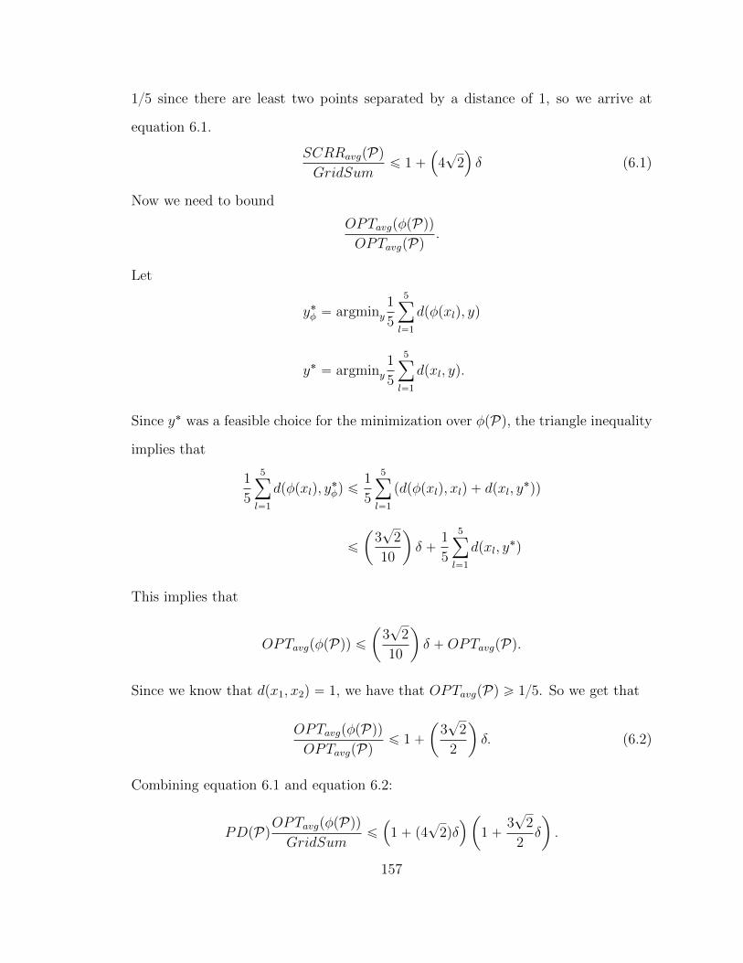
15 since there are least two points separated by a distance of 1, so we arrive at
equation 6.1.
SCRRavgpPqGridSum
ď 1`´
4?
2¯
δ (6.1)
Now we need to bound
OPTavgpφpPqqOPTavgpPq
.
Let
y˚φ “ argminy1
5
5ÿ
l“1
dpφpxlq, yq
y˚ “ argminy1
5
5ÿ
l“1
dpxl, yq.
Since y˚ was a feasible choice for the minimization over φpPq, the triangle inequality
implies that
1
5
5ÿ
l“1
dpφpxlq, y˚φq ď
1
5
5ÿ
l“1
pdpφpxlq, xlq ` dpxl, y˚qq
ď
ˆ
3?
2
10
˙
δ `1
5
5ÿ
l“1
dpxl, y˚q
This implies that
OPTavgpφpPqq ďˆ
3?
2
10
˙
δ `OPTavgpPq.
Since we know that dpx1, x2q “ 1, we have that OPTavgpPq ě 15. So we get that
OPTavgpφpPqqOPTavgpPq
ď 1`
ˆ
3?
2
2
˙
δ. (6.2)
Combining equation 6.1 and equation 6.2:
PDpPqOPTavgpφpPqqGridSum
ď
´
1` p4?
2qδ¯
ˆ
1`3?
2
2δ
˙
.
157

Now, suppose for a contradiction that PDpPq ě 1.97. Then we know that
GridSum
OPTavgpφpPqqě
1.97`
1` p4?
2qδ˘
´
1`´
3?2
2
¯
δ¯
So for δ :“ 175, we get that
GridSum
OPTavgpφpPqqě 1.781.
But φpPq Ă G, and computer analysis, searching over all possible configurations of
points on G, reveals no such configuration.
Lemma 20 provides the contradiction to our hypothesis and establishes Theo-
rem 25.
Discussion. Our analysis is slack in two ways: (1) we have to interpolate between
grid points, and (2) we consider pessimistic distortion over 5-tuples. Both are com-
putational constraints: (1) because we cannot simulate an arbitrarily fine grid, and
(2) because there is a combinatorial blow up in the search space when considering
larger tuples (note that by considering 5-tuples, we implicitly allow OPT to choose
a separate optimal solution for each 5-tuple). For Random Referee, the worst case
example found by computer simulations for grid points is fairly simple: The 5 points
lie on a straight line with pessimistic distortion 1.75. We conjecture the same exam-
ple is the worst case even in the continuous plane, which suggests a distortion bound
of at most 1.75. We leave finding the exact bound as an open question, as our result
is sufficient to demonstrate that comparison queries can take advantage of structure
that top-k queries cannot.
158

6.4 Favorite Only Mechanisms: Random Oligarchy
Recall that a favorite query asks an agent u P N for her favorite alternative pu. In
this section, we return to the general model (arbitrary metrics and not assuming
that dpu, puq “ 0) and study mechanisms that are restricted to only use favorite
queries. We show that essentially optimal Distortion as a function of |S| is achieved
by a simple mechanism that uses just 3 queries. We call this mechanism Random
Oligarchy.
Definition 21. The Random Oligarchy (RO) mechanism samples three agents u, v, w P
N independently and uniformly at random with replacement. All three are asked for
their favorite alternatives pu, pv, and pw in S. If the same alternative is reported at
least twice, output that, else output one of the three alternatives uniformly at random.
We prove that Random Oligarchy has the best of both worlds with respect to
the other favorite only mechanisms of Random Dictatorship and 2-Agree. Unlike
2-Agree, Random Oligarchy has constant sample complexity and the same Distor-
tion bound of 3 for large |S| as Random Dictatorship. However, like 2-Agree, it
outperforms Random Dictatorship for small |S|.
Theorem 26. The Distortion of Random Oligarchy is upper bounded by 3 for arbi-
trary |S|, and by the following expression for particular |S|.
1` 2 maxpPr0,1s
ˆ
1` p2pp´ 2q `pp´ 1q3
|S| ´ 1
˙
Proof. We analyze Random Oligarchy using a technical lemma proven in [85]. For
clarity of exposition, we restate the lemma.
Lemma 21. [85] The Distortion of any randomized mechanism f is less than or
equal to
1` 2 maxpPr0,1s
mf ppq1´ p
p
159
where mf ppq is the maximum probability of an alternative being output by f if exactly
a p fraction of N consider this alternative their top choice.
To apply Lemma 21, we need to bound mf ppq: the maximum probability of an
alternative being output by f if exactly a p fraction of N consider this alternative
their top choice (f , in this context, is just the Random Oligarchy mechanism). We
will first consider a coarse bound that allows us to upper bound Distortion by 3 for
arbitrary |S|, and will then consider a fine grained bound that takes |S| into account.
It is straightforward from Definition 21 that Random Oligarchy outputs an alter-
native x P S only if (i) it draws at least two agents who report x as their favorite,
or if (ii) all three agents drawn report different favorite alternatives, and x is among
them, in which case it is output with probability 13. Given that exactly a p fraction
of N consider such an x as their top choice, it is straightforward to compute (i). A
coarse upper bound on the probability of (ii) is`
31
˘
pp1 ´ pq2, the probability that
the alternative in question is reported exactly once, and something else is reported
for the other two draws. This is potentially an overestimate, since these two other
alternatives reported must be distinct, but ignoring this detail gives the following
coarse bound on mf ppq.
mf ppq ď
ˆ
3
3
˙
p3 `
ˆ
3
2
˙
p2p1´ pq `1
3
ˆ
3
1
˙
pp1´ pq2
“ ´p3 ` p2 ` p
Inserting this into Lemma 21 and simplifying shows that the Distortion of Random
Oligarchy is at most 3.
Distortionpfq ď 1` 2 maxpPr0,1s
ˆ
`
´p3 ` p2 ` p˘ 1´ p
p
˙
“ 3
To obtain a more fine grained bound that considers |S|, note that the probability
of (ii) is maximized when the distribution over favorite points of all agents who do
160
not report x as their favorite is uniform over the remaining |S| ´ 1 alternatives.
Taking into account that for event (ii) the two other reported alternatives must be
unique yields the following bound on mf ppq.
mf ppq ď
ˆ
3
3
˙
p3 `
ˆ
3
2
˙
p2p1´ pq
`1
3
ˆ
3
1
˙
pp1´ pq
ˆ
1´ p´1´ p
|S| ´ 1
˙
“ ´p3 ` p2 ` p´ppp´ 1q2
|S| ´ 1
Substituting this expression into Lemma 21 allows us to upper bound the Distortion
of Random Oligarchy by
1` 2 maxpPr0,1s
ˆˆ
´p3 ` p2 ` p´ppp´ 1q2
|S| ´ 1
˙
1´ p
p
˙
.
Simplifying yields the theorem statement.
Figure 6.2 shows the Distortion bounds of favorite only mechanisms. Comparing
against the lower bound for any favorite only mechanism from [85] allows us to see
that Random Oligarchy is essentially optimal among all favorite only mechanisms.
In comparison to existing mechanisms, Random Oligarchy outperforms Random Dic-
tatorship for small |S|, and outperforms 2-Agree for large |S|, while only using three
favorite queries.
6.5 Conclusion and Open Directions
In this chapter, we studied constant sample complexity mechanisms for implicit util-
itarian social choice. We proposed two mechanisms: Random Referee and Random
Oligarchy, for achieving constant Distortion and Squared Distortion bounds using a
constant number of simple ordinal queries. At a high level, we hope that our work
161

Figure 6.2: Distortion of Favorite Only Mechanisms. Upper bounds for Ran-dom Oligarchy are from Theorem 26. Lower bounds and 2-Agree upper bounds arefrom [85]. Random Dictatorship is analyzed in [8].
inspires future research on lightweight mechanisms for social choice in large decision
spaces. We also mention some natural technical questions raised by our work.
Compared to Distortion, there is much less understanding of the Squared Distor-
tion of mechanisms. The only universal lower bound for Squared Distortion we are
aware of is 4, a consequence of the lower bound of 2 for Distortion [8]. Our Random
Referee mechanism achieves Squared Distortion of at most 21 using just three ordinal
queries. Closing this gap remains an interesting question even for mechanisms that
elicit full ordinal information.
The analysis in Section 6.3 of Random Referee generalizes to higher dimensional
Euclidean space, still only reasoning about 5-tuples of points. Computer search
over a coarse grid in four dimensions again shows that the pessimistic distortion
bound is better than 2. However, we have not been able to run the search on a fine
enough grid to prove a Distortion bound formally. We leave proving this for higher
dimensional Euclidean spaces as an interesting open question. Additionally, we hope
that related methods may be of general interest for proving tighter Distortion bounds
of mechanisms on restricted metric spaces.
It remains unclear whether using a constant number of queries greater than 3
162

would meaningfully improve our results. E.g., consider the natural extension of Ran-
dom Referee: sample the favorite points of k agents and ask a random referee to
choose their favorite from among these. Using k ą 2 does not straightforwardly de-
crease the Squared Distortion bound of 21 for k = 2. Also, as k becomes large, this
mechanism devolves to Random Dictatorship. Another natural question is whether
Opkq comparison queries are necessary/sufficient to bound the k’th moment of Dis-
tortion. We leave these as additional open questions.
163

7
Conclusion
We have studied public decision making as an algorithmic discipline from two broad
perspectives: fairness in the allocation of public goods, and implicit utilitarian social
choice. Our primary results in fair resource allocation have involved a deep explo-
ration of the computation of core solutions to fair resource allocation problems, a
novel fairness notion that generalizes the idea of proportionality by explicitly consid-
ering fairness with respect to subsets of agents in order to account for the potential
for sharing public goods. These algorithms provide strong guarantees on fairness and
efficiency for problems including budgeting, memory sharing, multiple referendums,
multi-winner elections, and centroid clustering. In implicit utilitarian social choice,
we designed a sequential protocol based on iterative Nash bargaining, and one shot
protocols based on a simple and restricted query model, in order to provide constant
Distortion guarantees (approximation to the social optimum). We also extended
existing work by considering additional desiderata, most notably the Squared Dis-
tortion. These are lightweight protocols for social choice where there is a large space
of alternatives.
In addition to many outstanding technical questions mentioned in specific chap-
164

ters, there are some important broad questions that I wish to highlight in closing.
First, we have only occasionally considered issues of strategic behavior, that is, the
possibility that agents might misreport their true preferences in order to manipu-
late our algorithms to their advantage. The free rider problem is perhaps the most
famous argument that public decision making is impeded by strategic concerns. In
particular, for most of the problems considered in public decision making, the indi-
vidual agents have an incentive to pretend to be disinterested in shared public goods,
and instead feign interest only in more niche private goods.
This problem seems endemic in the allocation of public goods. There are classic
impossibility results regarding strategic behavior, including the Gibbard-Satterthwaite
impossibility theorem in ordinal voting [78], and the Myerson-Satterthwaite impos-
sibility theorem in mechanism design [129]. These results are of the form that no
voting rule or mechanism can simultaneously satisfy three or four desirable axioms,
one of which is a form of truthfulness: that agents should not have an incentive to
misreport their preferences.
Nevertheless, I believe there are important approaches for sidestepping some of
these impossibilities. These ideas are based on approximation of two types. The first
is to design mechanisms that may not be exactly truthful, but for which an agent
cannot increase her expected utility by a large factor by misreporting her prefer-
ences. We have already seen this approach to mechanism design with the exponential
mechanism of Section 2.3.2. Another approach is to accept that agents may behave
strategically, and design algorithms for which other desirable properties (such as fair-
ness, or welfare maximization) are still approximately obtained, even when agents
so behave. This, for example, is the basic idea behind analysis of the price of an-
archy [109]. I hope to more fully explore the application of these approaches to
designing more strategically robust algorithms for public decision making.
Another relatively unexplored area of research concerns the true nature of many
165

application domains in public decision making as problems of mixed public goods and
“bads” (also sometimes called “chores” in the literature). In every chapter, we have
either assumed that we are exclusively dealing with public goods (for which agents
only have nonnegative utility) or exclusively dealing with public bads (in particular,
in Chapters 4 through 6 we supposed that public outcomes had costs for agents).
However, in reality, many public outcomes are good for some and bad for others. For
example, building a highway through a neighborhood may be good to those who use
the highway, but bad to those who live in the neighborhood.
This also seems to be a fundamental problem in much of the current literature
on fair machine learning, including problems like predicting loan default, predictive
policing, and recommender systems. I believe that algorithmic fairness in such a con-
text demands considering a rich diversity of preferences over outcomes that may differ
among the individuals and between the subjects and designers of the systems. Such
an approach may allow one to go beyond statements about marginals of predictive
distributions and instead make statements about the impact of algorithms on indi-
viduals. Normative utilitarian theory and corresponding algorithms may have much
to contribute to this emerging field, but such work may need to account for mixed
goods and bads present in many of these problems with fundamental developments
in terms of solution concepts and computation.
At a higher level, our discussion has been characterized by a deep interaction be-
tween normative economics and developing efficient approximation algorithms with
provable guarantees. This intersection between the normative and algorithmic (what
is the right solution concept, and how can we compute it?) has obvious and tradi-
tional applications in voting and budgeting. But, this intersection is also significant
in an age when machine intelligence is rapidly being deployed within regular human
society. For better or for worse, algorithm designers will find themselves engaged in
projects with substantial normative questions like machine learning driven algorith-
166

mic decision making, autonomous vehicles, social robotics, and many more projects
that I cannot hope to predict. Thinking critically about the right solution concepts
for these problems can either be done cursorily and after-the-fact, viewed as a distrac-
tion from the design of more efficient algorithms, or it can be seen as a fundamental
part of algorithm design. It is my hope that this thesis contributes toward a future
that takes the latter approach, for the public good of all.
167
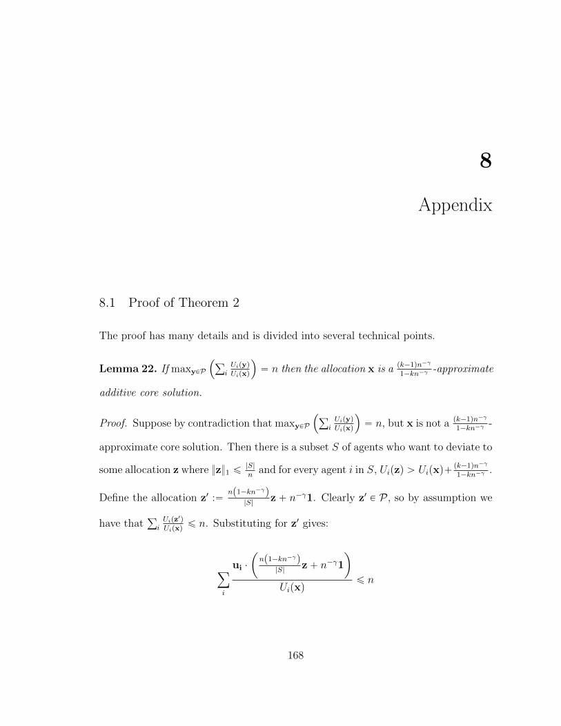
8
Appendix
8.1 Proof of Theorem 2
The proof has many details and is divided into several technical points.
Lemma 22. If maxyPP
´
ř
iUipyqUipxq
¯
“ n then the allocation x is a pk´1qn´γ
1´kn´γ-approximate
additive core solution.
Proof. Suppose by contradiction that maxyPP
´
ř
iUipyqUipxq
¯
“ n, but x is not a pk´1qn´γ
1´kn´γ-
approximate core solution. Then there is a subset S of agents who want to deviate to
some allocation z where z1 ď|S|n
and for every agent i in S, Uipzq ą Uipxq`pk´1qn´γ
1´kn´γ.
Define the allocation z1 :“np1´kn´γq
|S|z ` n´γ1. Clearly z1 P P , so by assumption we
have thatř
iUipz
1q
Uipxqď n. Substituting for z1 gives:
ÿ
i
ui ¨
ˆ
np1´kn´γq|S|
z` n´γ1
˙
Uipxqď n
168

Thus, solving forř
iui¨zUipxq
and simplifying:
ÿ
i
ui ¨ z
Uipxqď
|S|
n p1´ kn´γq
˜
n´ÿ
i
n´γ
Uipxq
¸
ď1´ n´γ
1´ kn´γ|S|
However, recall that since S is a deviating coalition from the approximate core, it
should be that Uipzq ą Uipxq `pk´1qn´γ
1´kn´γfor all agents i P S. This implies that for all
i P S, it should be that UipzqUipxq
ą 1 ` pk´1qn´γ
1´kn´γ. Thus, we can bound the sum over i as
ř
iUipzqUipxq
ą 1´n´γ
1´kn´γ|S|. This is a contradiction, completing the proof.
Using essentially the same argument, the following corollary follows easily.
Corollary 6. If maxyPP
´
ř
iUipyqUipxq
¯
“ n`α then the allocation x is an pk´1qn´γ`αn´1
1´kn´γ-
approximate additive core solution.
Lemma 23. qpxq ě 0 and maxxPP qpxq “ n ´ n1´γ. Further, if ∆q is the largest
possible difference in the scoring function between two sets of input differing only on
the report of a single agent i1, (i.e., the sensitivity of q), then ∆q “ 1.
Proof. To see the first part, note that Uipxq ě n´γ for all x P P . Therefore,
qpxq “ n´ n´γ maxyPP
˜
ÿ
i
Uipyq
Uipxq
¸
ě n´ n´γÿ
i
1
n´γ“ 0
By the optimality condition of the Proportional Fairness convex program,
minxPP
maxyPP
˜
ÿ
i
Uipyq
Uipxq
¸
“ n
Therefore, maxxPP qpxq “ n´ n1´γ. Similarly, when agent i1 misreports:
∆q “
ˇ
ˇ
ˇ
ˇ
ˇ
˜
n´ n´γ maxyPP
˜
ÿ
i
Uipyq
Uipxq
¸¸
´
˜
n´ n´γ maxyPP
˜
Ui1pyq
Ui1pxq`ÿ
i‰i1
Uipyq
Uipxq
¸¸ˇ
ˇ
ˇ
ˇ
ˇ
ď n´γˆ
maxyPP
ˆ
Ui1pyq
Ui1pxq
˙
´ 1
˙
ď 1
169

The first inequality follows because we can assume w.l.o.g. that if the maximizing
y changed for the misreported data, it yields a score no worse than the score of the
original y on the misreported data, since that original y could have been chosen.
Exponential Mechanism We now plug the above scoring function into the Exponential
mechanism from [123]. We use ε ą 0 as the privacy approximation parameter, and
thus as a parameter for the approximation of truthfulness.
Definition 22. Define µ to be a uniform probability distribution over all feasible
allocations x P P. For a given set of utilities, let the mechanism ζεq be given by the
rule:
ζεq :“ choose x with probability proportional to eεqpxqµpxq
The following lemma follows by using the sensitivity bound from Lemma 23 in
Theorem 6 from [123].
Lemma 24. ζεq is pe2ε ´ 1q-approximately truthful.
Finally, we demonstrate that ζεq can still find an approximate core solution while
providing approximate truthfulness, establishing Theorem 2.
Claim 3. If k is op?nq and 1
εą kn
pn´k2q lnnthen ζεq can be used to choose an allocation
x that is an O´
k lnnε?n
¯
-approximate additive core solution w.p. 1´ 1n
.
Proof. Let t “ k`1ε
lnn. Lemma 7 in [123] states that
Pr
«
n´ n´γ maxyPP
˜
ÿ
i
Uipyq
Uipxq
¸
ď OPT ´ 2t
ff
ďe´εt
µpStq(8.1)
where OPT is the maximum value of qpxq for feasible allocations x and St “ tx :
qpxq ą OPT ´ tu. By Lemma 23, we have OPT “ np1´n´γq, but we need to bound
170

µpStq, the probability that x drawn uniformly at random from P is in St. We will
show that µpStq ě n´k. Let x˚ P P be the allocation such that qpx˚q “ OPT . Since
x1 “ 1, there is an item j1 with x˚j1 ě 1k. Let δ “ 1n. Define the set Sδ so that
Sδ “
$
&
%
x :x˚j ď xj ď x˚j ` δ j ‰ j1
x˚j1 ´ k2δx˚j1 ď xj1 ď x˚j1 ´ k
2δx˚j1 ` δ j “ j1
,
.
-
It is not hard to see that since x˚j1 ě 1k, all x P Sδ are feasible. Furthermore, because
there is a “width” of 1n in possible choice of xj for all j, µpSδq ě n´k. Thus, to
complete the argument that µpStq ě n´k, we just need to show that Sδ Ď St. In our
case,
St “
#
x : maxyPP
ÿ
i
Uipyq
Uipxqă n`
k ` 1
εlnn
+
Since 1εą kn
pn´k2q lnn, substituting shows that an allocation x is surely in St if the
same sum is less than n2
n´k2. By construction, in the worst case for any agent i and
allocation x P Sδ (namely, if uij1 “ 1), Uipxq ěn´k2
nUipx
˚q. Therefore, for all x P Sδ
maxyPP
ÿ
i
Uipyq
Uipxqď
n
n´ k2maxyPP
ÿ
i
Uipyq
Uipx˚q“
n2
n´ k2
Thus, we have that Sδ Ď St and therefore µpStq ě n´k. Substituting into equa-
tion 8.1 and simplifying yields
Pr
«
maxyPP
˜
ÿ
i
Uipyq
Uipxq
¸
ą n` 2k ` 1
εnγ lnn
ff
ď1
n
By applying Corollary 6, we get that x chosen according to ζεq is a pk´1qn´γ`2pk`1qε´1nγ´1 lnn1´kn´γ
-
approximate core solution with probability 1´ 1n. Plugging in γ “ 12 and using the
fact that k is op?nq gives that x chosen according to ζεq is an O
´
k lnnε?n
¯
-approximate
core solution with probability 1´ 1n.
171

8.2 Proof of Theorem 8
The fractional outcome maximizing the Nash welfare objective is the solution of the
following program. For simplicity of presentation, we absorb the constraint that
wj ď 1 for each j P W into the packing constraints.
Maximizeÿ
iPN
lnUi (8.2)
řmj“1 akjwj ď bk @k P rKs
Ui “řmj“1wjuij @i P N
wj ě 0 @j P W
Denote a vector of utilities by U “ xU1, U2, . . . , Uny, and the polytope of feasible
utility vectors by U . Then, the fractional MNW outcome is obtained by the following
maximization.
maxUPU
ÿ
iPN
lnUi (8.3)
We want to compute a fractional pδ, εq-approximate core outcome in time poly-
nomial in n, Vmax, and log 1δε
. Assume that U is a convex polytope of feasible utility
vectors. For any δ ě 0, ε ą 0, let ε1 “ εp1 ` δq. Define the following objective
function. Note that in the absence of the ε1 term, it would mimic the derivative of
the Nash social welfare objective from Program (8.3).
minUPU
QpUq, where QpUq “ maxU1PU
ÿ
iPN
U 1i ` ε1
Ui ` ε1. (8.4)
Clearly, QpUq ě n for every U. Thus, the objective value in Program (8.4) is
at least n. In Section 3.2.2, we presented an argument showing that the fractional
172

MNW outcome is in the core. A similar argument using the first order optimality
condition shows that if U˚ P arg maxUPUř
iPN lnpUi ` ε1q, then
ÿ
iPN
Ui ` ε1
U˚i ` ε1ď n.
This implies the optimum of Program (8.4) is achieved at the fractional outcome
maximizing the smooth Nash welfare objectiveř
iPN lnpUi ` ε1q, and this optimal
value is exactly n.
Next, we turn to efficiently approximating Program (8.4), and show that if
QpUq ď np1` δq, then U is a pδ, εq-core outcome.
We want to use the Ellipsoid algorithm to approximately minimize the objective
function QpUq over U P U in polynomial time. For this, all we need is that Q is
a convex function, its subgradient is efficiently computable, the range of Q and the
diameter of U are exponentially bounded, and polytope U is efficiently separable [35].
First, we claim that QpUq is a convex function of U. To see this, note that for
any fixed U1, U 1iUi is convex in Ui. Since the sum and maximum of convex functions
is convex, we conclude that QpUq is also convex.
Second, the subgradient of QpUq is efficiently computable for every U P U . First,
we find the U1 P U that maximizesř
iPNU 1i`ε
1
Ui`ε1by solving a linear program. Then,
we fix U1 and take the gradient ofU 1iUi
with respect to Ui to obtain a subgradient of
QpUq.
Third, note that Ui P r0, Vmaxs for each i. Hence, QpUq ď n¨pVmax`ε1qε1
, which is
exponentially bounded in the input size. It is easy to see that the same holds for the
diameter of the polytop U .
Finally, polytope U is efficiently separable because it is a set of polynomially
many linear inequalities.
173

Hence, we can efficiently obtain a solution U P U that satisfies
maxU1PU
ÿ
iPN
U 1i ` ε1
Ui ` ε1ď n` δ ď np1` δq.
Finally, we show that U must be a pδ, εq-core outcome. Suppose for contradiction
that it is not. Then, there exists a subset S of agents and an outcome U1 such that
p1` δq ¨ Ui ` ε ď|S|
n¨ U 1i
for all i P S, and at least one inequality is strict. Rearranging the terms and summing
over i P S, we obtain
ÿ
iPS
U 1i
p1` δq ¨ Ui ` εą |S| ¨
n
|S|“ n.
However, we also have
ÿ
iPS
U 1i
p1` δq ¨ Ui ` εďÿ
iPS
U 1i ` ε1
p1` δq ¨ pUi ` ε1q“
1
1` δ
ÿ
iPS
U 1i ` ε1
Ui ` ε1ď n,
where the last inequality is due to approximate optimality of U. This is a contra-
diction. Hence, U is a pδ, εq-core outcome.
8.3 Proof of Lemma 10
First, we give a brief overview of the method from [43]. Note that our goal in this
argument is to show that the new constraint we added (constraint 4.6) is approxi-
mately satisfied after this rounding. The authors work in a setting where points can
have demand. In our setting, this just corresponds to points in N having a demand
of 1, and moving or consolidating demand can be thought of as changing the instance
by moving points in N . Note that the original linear program requires N ĎM, and
we follow suit in this proof.
174

Given a fractional solution to the linear program in Figure 4.3 as tyju, tziju, let
Ci “ř
jPM dpi, jqzij. That is, Ci is the contribution of point i to the k-median
objective in the fractional optimum.
• Step 1: Consolidate all demands ti to obtain tt1iu such that for all i, j PM with
t1i ą 0, t1j ą 0, they must be sufficiently far away such that cij ą 4 maxpCi, Cjq.
Let M1 be the set of centers with positive demand after this step, i.e. M1 “
tj PM : t1j ą 0u.
• Step 2a: Consolidate open centers by moving each center not in M1 to the
nearest center in M1. This gives a new solution ty1ju, tz1iju with y1j ě
12
if
j PM1 and y1j “ 0 if j RM1. We call this a 12-restricted solution.
• Step 2b: Modify the solution further to obtain tyju, tziju with yj P t12, 1u if
j PM1 and yj “ 0 if j RM1. We call this a t12, 1u-integral solution.
• Step 3: Round tyju, tziju to obtain an integer solution tyju, tziju.
We introduce constraint 4.6 in our linear program, and make a small modification
to Step 2b as described in sections below.
8.3.1 Step 1: Consolidating Demands
Our first observation is that during the demand consolidation, it cannot be the
case that all of the demand within a given Bpi, γRiq from constraint 4.6 is moved
arbitrarily far away.
Lemma 25. Fix i P M. For each j P Bpi, γRiq that had its demand moved to
j1 PM1, dpi, j1q ď 9γRi.
Proof. Let j P Bpi, γRiq. Let j1 be the location to which the demand for j was
moved in Step 1. Note that Step 1 is designed so that if demand at j is moved to
175

another point j1, then Cj1 ď Cj, and cjj1 ď 4 maxpCj, Cj1q “ 4Cj. By constraint 4.6,
we know that the demand of j could be completely satisfied by centers fractionally
opened inside of Bpi, γRiq, so Cj ď 2γRi ùñ cjj1 ď 8γRi. Since j P Bpi, γRiq, it
follows that dpi, j1q ď 9Ri.
8.3.2 Step 2: Consolidating Centers
Next, we argue that the consolidation of fractional centers in Step 2 approximately
preserves constraint 4.6.
Lemma 26. After Step 2a, @j PM,ř
j1PBpj,9γRjqy1j1 ě 1.
Proof. Consider each location j1 P Bpj, γRjq. Let j2 be the location in M1 closest
to j1. By Lemma 25, there exists such a j2 with dpj, j2q ď 9γRj, so j2 P Bpj, 9γRjq.
Step 2a will move the fractional center at j1 to j2, so y1j2 ě minp1, yj1 ` yj2q ě yj1 .
Summing over all j1 P Bpj, γRjq, we haveř
j2PBpj,9γRjqy1j2 ě
ř
j1PBpj,γRjqy1j ě 1 by
constraint 4.6.
For our algorithm, we slightly change Step 2b to the following: Let M2 “ tj P
M1 : y1j ă 1u, m1 “ |M1| and m2 “ |M2|. Sort the locations j PM2 in decreasing
order of t1jdpspjq, jq, where spjq is the location in M1 closest to j (other than j). Set
yj “ 1 for the first 2k ´ 2m1 ` m2 locations in M2 or if j P M1zM2, and yj “12
otherwise. In other words, the only difference from the original Step 2b in [43] is that
points with integral y1j “ 1 will not participate in the sorting; we simply set yj “ 1 for
such points, and then perform the standard rounding on M2. [43] use the following
statement in their proof, and we show that it still holds after our modification to
Step 2b.
Lemma 27. For any 12-restricted solution ty1ju, tz
1iju, the modified Step 2b givs a
t12, 1u-integral solution with no greater cost.
176

Proof. From Lemma 7 in [43], the cost of the 12-restricted solution ty1ju, tz
1iju is
ÿ
jPM1
t1j`
1´ y1j˘
dpspjq, jq
“ÿ
jPM2
t1j`
1´ y1j˘
dpspjq, jq
“ÿ
jPM2
t1jdpspjq, jqq ´ÿ
jPM2
t1jdpspjq, jqy1j.
where the second line follows because y1j “ 1 @j P M1zM2. Our algorithm in Step
2b maximizesř
jPM2 t1jdpspjq, jqyj for the given set of t1jdpspjq, jq, hence achieves a
cost at most that of ty1ju, tz1iju.
Lemma 28. After Step 2b, @j PM, there is either at least one j1 P Bpj, 9γRjq with
yj1 “ 1 or at least two j1 P Bpj, 9γRjq with yj1 ě12.
Proof. Given Lemma 26 and the constraints on y1i after Step 2a, there must be at
least one j1 P Bpj, 9γRjq with positive demand. If there is exactly one such j1,
Lemma 3 is equivalent to y1j1 “ 1 and Step 2b will ensure yj1 “ 1. If there are at
least two such j1, all of them will have yj1 ě12
after Step 2b.
8.3.3 Step 3: Rounding an Integer Solution
[43] gives two rounding schemes, and we use the first one that at most doubles the
cost. The important observation is that any center with yj “ 1 will be opened in
the integral solution (that is, if yj “ 1 then yj “ 1, and for any center with yj “12,
either j itself or another center in M1 closest to j will be opened. This allows us to
complete our argument.
Lemma 29. For all j PM,ř
j1PBpj, 27γRjqyj1 ě 1.
Proof. By Lemma 28, there are two cases: either there is some j1 P Bpj, 9γRjq with
yj1 “ 1 or there are at least two j1 P Bpj, 9γRjq with yj1 ě12. In the first case,
177

yj1 “ yj1 “ 1, so the lemma statement clearly holds. In the second case, we are
guaranteed that for each point j1, either we set yj1 “ 1 (in which case the Lemma
holds) or we set yj2 “ 1 where j2 is the closest other at least partially open center.
But since in this case there are two points in Bpj, 9γRjq partially open, their pairwise
distance is at most 18γRj, so dpj1, j2q ď 18γRj ùñ dpj, j2q ď 27γRj.
This concludes the proof of Lemma 10. The fact that tyju, tziju is an 8-approximation
of the objective follows immediately from the proof from [43] given Lemma 27, as all
other constraints are still satisfied. Finally, we note that the constant factor of 27
can be tightened to 13 in the special case where N “M. The argument is essentially
the same. The crucial improvement comes from the guarantee that @i P M, there
is demand at the center of each Bpi, γRiq. Tracking this demand throughout the
rounding leads to the tightened result.
178

Bibliography
[1] The participatory budgeting project. https://www.
participatorybudgeting.org.
[2] Abramowitz, B., and Anshelevich, E. Utilitarians without utilities:Maximizing social welfare for graph problems using only ordinal preferences.In Proceedings of the Thirty-Second AAAI Conference on Artificial Intelligence(2018), AAAI Press, pp. 894–901.
[3] Airiau, S., Aziz, H., Caragiannis, I., Kruger, J., and Lang, J. Po-sitional social decision schemes: Fair and efficient randomized portioning. InProceedings of the 7th International Workshop on Computational Social Choice(COMSOC) (2018).
[4] Airiau, S., and Endriss, U. Iterated majority voting. In InternationalConference on Algorithmic Decision Theory (2009), Springer, pp. 38–49.
[5] Amanatidis, G., Markakis, E., Nikzad, A., and Saberi, A. Approx-imation algorithms for computing maximin share allocations. ACM Transac-tions on Algorithms 13, 4 (Dec. 2017), 52:1–52:28.
[6] Anari, N., Oveis Gharan, S., Saberi, A., and Singh, M. Nash SocialWelfare, Matrix Permanent, and Stable Polynomials. In Proceedings of the8th Innovations in Theoretical Computer Science Conference (ITCS) (2017),pp. 36:1–36:12.
[7] Anshelevich, E., Bhardwaj, O., Elkind, E., Postl, J., andSkowron, P. Approximating optimal social choice under metric preferences.Artificial Intelligence 264 (2018), 27 – 51.
[8] Anshelevich, E., and Postl, J. Randomized social choice functions undermetric preferences. Journal of Artificial Intelligence Research 58, 1 (2017),797–827.
179

[9] Anshelevich, E., and Zhu, W. Ordinal approximation for social choice,matching, and facility location problems given candidate positions. In The14th Conference on Web and Internet Economics (WINE) (2018), Springer,pp. 3–20.
[10] Arora, S., Hazan, E., and Kale, S. The multiplicative weights updatemethod: a meta-algorithm and applications. Theory of Computing 8, 6 (2012),121–164.
[11] Arrow, K. J. A difficulty in the concept of social welfare. Journal of PoliticalEconomy 58, 4 (1950), 328–346.
[12] Arthur, D., and Vassilvitskii, S. K-means++: The advantages of carefulseeding. In Proceedings of the Eighteenth Annual ACM-SIAM Symposium onDiscrete Algorithms (SODA) (2007), pp. 1027–1035.
[13] Arya, V., Garg, N., Khandekar, R., Meyerson, A., Munagala, K.,and Pandit, V. Local search heuristics for k-median and facility locationproblems. SIAM Journal on Computing 33, 3 (2004), 544–562.
[14] Azevedo, E. M., and Budish, E. Strategyproofness in the large as adesideratum for market design. In EC (2012), pp. 55–55.
[15] Aziz, H., Brandl, F., and Brandt, F. On the incompatibility of effi-ciency and strategyproofness in randomized social choice. In Proceedings ofthe Twenty-Eighth AAAI Conference on Artificial Intelligence (2014), AAAIPress, pp. 545–551.
[16] Aziz, H., Brill, M., Conitzer, V., Elkind, E., Freeman, R., andWalsh, T. Justified representation in approval-based committee voting. SocialChoice and Welfare 48, 2 (2017), 461–485.
[17] Aziz, H., Elkind, E., Huang, S., Lackner, M., Fernandez, L. S.,and Skowron, P. On the complexity of extended and proportional justi-fied representation. In Proceedings of the Thirty-Second AAAI Conference onArtificial Intelligence (2018), AAAI Press, pp. 902–909.
[18] Aziz, H., and Mackenzie, S. A discrete and bounded envy-free cake cuttingprotocol for any number of agents. In Proceedings of the 57th Annual IEEESymposium on Foundations of Computer Science (FOCS) (2016), pp. 416–427.
[19] Aziz, H., and Mackenzie, S. A discrete and bounded envy-free cake cut-ting protocol for four agents. In Proceedings of the Forty-eighth Annual ACMSymposium on Theory of Computing (STOC) (2016), ACM, pp. 454–464.
180

[20] Bandelt, H.-J., and Barthelemy, J.-P. Medians in median graphs. Dis-crete Applied Mathematics 8, 2 (1984), 131 – 142.
[21] Barbera, S., Gul, F., and Stacchetti, E. Generalized median voterschemes and committees. Journal of Economic Theory 61, 2 (1993), 262 – 289.
[22] Barman, S., Biswas, A., Krishnamurthy, S., and Narahari, Y.Groupwise maximin fair allocation of indivisible goods. In Proceedings of theThirty-Second AAAI Conference on Artificial Intelligence (2018), AAAI Press,pp. 917–924.
[23] Barman, S., and Krishna Murthy, S. K. Approximation algorithmsfor maximin fair division. In Proceedings of the 2017 ACM Conference onEconomics and Computation (EC) (2017), ACM, pp. 647–664.
[24] Barman, S., Krishnamurthy, S. K., and Vaish, R. Greedy algorithmsfor maximizing nash social welfare. In Proceedings of the 17th InternationalConference on Autonomous Agents and MultiAgent Systems (AAMAS) (2018),pp. 7–13.
[25] Benade, G., Nath, S., Procaccia, A. D., and Shah, N. Preferenceelicitation for participatory budgeting. In Proceedings of the Thirty-First AAAIConference on Artificial Intelligence (2017), AAAI Press, pp. 376–382.
[26] Bennett, E., and Houba, H. Odd man out: Bargaining among threeplayers. Working Papers 662, UCLA Department of Economics, May 1992.
[27] Bhaskar, U., Dani, V., and Ghosh, A. Truthful and near-optimal mech-anisms for welfare maximization in multi-winner elections. In Proceedings ofthe Thirty-Second AAAI Conference on Artificial Intelligence, pp. 925–932.
[28] Binmore, K., Rubinstein, A., and Wolinsky, A. The nash bargainingsolution in economic modelling. The RAND Journal of Economics 17, 2 (1986),176–188.
[29] Binmore, K., Shaked, A., and Sutton, J. Testing noncooperative bar-gaining theory: A preliminary study. The American Economic Review 75, 5(1985), 1178–1180.
[30] Bolukbasi, T., Chang, K.-W., Zou, J. Y., Saligrama, V., and Kalai,A. T. Man is to computer programmer as woman is to homemaker? debias-ing word embeddings. In Advances in Neural Information Processing Systems(NIPS). 2016, pp. 4349–4357.
181

[31] Boutilier, C., Caragiannis, I., Haber, S., Lu, T., Procaccia, A. D.,and Sheffet, O. Optimal social choice functions: A utilitarian view. Arti-ficial Intelligence 227 (2015), 190–213.
[32] Bouveret, S., Chevaleyre, Y., Durand, F., and Lang, J. Voting bysequential elimination with few voters. In Proceedings of the Twenty-Sixth In-ternational Joint Conference on Artificial Intelligence (IJCAI) (2017), pp. 128–134.
[33] Brandl, F., Brandt, F., Eberl, M., and Geist, C. Proving the incom-patibility of efficiency and strategyproofness via smt solving. Journal of theACM 65, 2 (2018), 6:1–6:28.
[34] Brandt, F., Conitzer, V., Endriss, U., Lang, J., and Procaccia,A. D. Handbook of Computational Social Choice, 1st ed. Cambridge UniversityPress, 2016.
[35] Bubeck, S. Convex optimization: Algorithms and complexity. Foundationsand Trends in Machine Learning 8, 3-4 (2015), 231–357.
[36] Buchfuhrer, D., Schapira, M., and Singer, Y. Computation and in-centives in combinatorial public projects. In Proceedings of the 11th ACMConference on Electronic Commerce (2010), ACM, pp. 33–42.
[37] Budish, E. The combinatorial assignment problem: Approximate competitiveequilibrium from equal incomes. Journal of Political Economy 119, 6 (2011),1061 – 1103.
[38] Cabannes, Y. Participatory budgeting: a significant contribution to partici-patory democracy. Environment and Urbanization 16, 1 (2004), 27–46.
[39] Cai, Y., Daskalakis, C., and Weinberg, S. M. Understanding incen-tives: Mechanism design becomes algorithm design. In Proceedings of the 54thAnnual IEEE Symposium on Foundations of Computer Science (FOCS) (2013),pp. 618–627.
[40] Caliskan, A., Bryson, J. J., and Narayanan, A. Semantics derivedautomatically from language corpora contain human-like biases. Science 356,6334 (2017), 183–186.
[41] Caragiannis, I., Kurokawa, D., Moulin, H., Procaccia, A. D.,Shah, N., and Wang, J. The unreasonable fairness of maximum nash wel-fare. In Proceedings of the 2016 ACM Conference on Economics and Compu-tation (EC) (2016), ACM, pp. 305–322.
182
[42] Caragiannis, I., and Procaccia, A. D. Voting almost maximizes socialwelfare despite limited communication. In Proceedings of the Twenty-FourthAAAI Conference on Artificial Intelligence (2010), AAAI Press, pp. 743–748.
[43] Charikar, M., Guha, S., va Tardos, and Shmoys, D. B. A constant-factor approximation algorithm for the k-median problem. Journal of Com-puter and System Sciences 65, 1 (2002), 129 – 149.
[44] Chen, X., Dai, D., Du, Y., and Teng, S.-H. Settling the Complexityof Arrow-Debreu Equilibria in Markets with Additively Separable Utilities. InProceedings of the 50th Annual IEEE Symposium on Foundations of ComputerScience (FOCS) (2009), pp. 273–282.
[45] Chen, X., Fain, B., Lyu, L., and Munagala, K. Proportionally fairclustering. Manuscript under review at the the 36th International Conferenceon Machine Learning (ICML).
[46] Cheng, Y., Dughmi, S., and Kempe, D. Of the people: Voting is moreeffective with representative candidates. In Proceedings of the 2017 ACM Con-ference on Economics and Computation (EC) (2017), ACM, pp. 305–322.
[47] Chierichetti, F., Kumar, R., Lattanzi, S., and Vassilvitskii, S. Fairclustering through fairlets. In Advances in Neural Information Processing Sys-tems (NIPS). 2017, pp. 5029–5037.
[48] Clearwater, A., Puppe, C., and Slinko, A. Generalizing the single-crossing property on lines and trees to intermediate preferences on mediangraphs. In Proceedings of the 24th International Conference on Artificial In-telligence (IJCAI) (2015), pp. 32–38.
[49] Cole, R., Devanur, N., Gkatzelis, V., Jain, K., Mai, T., Vazirani,V. V., and Yazdanbod, S. Convex program duality, fisher markets, andnash social welfare. In Proceedings of the 2017 ACM Conference on Economicsand Computation (EC) (2017), ACM, pp. 459–460.
[50] Cole, R., and Gkatzelis, V. Approximating the nash social welfare withindivisible items. In Proceedings of the Forty-seventh Annual ACM Symposiumon Theory of Computing (STOC) (2015), ACM, pp. 371–380.
[51] Cole, R., Gkatzelis, V., and Goel, G. Mechanism design for fair divi-sion: Allocating divisible items without payments. In Proceedings of the Four-teenth ACM Conference on Electronic Commerce (EC) (2013), ACM, pp. 251–268.
183

[52] Collins, F. S., and Varmus, H. A new initiative on precision medicine.New England Journal of Medicine 372, 9 (2015), 793–795.
[53] Conitzer, V., Freeman, R., and Shah, N. Fair public decision making.In Proceedings of the 2017 ACM Conference on Economics and Computation(EC) (2017), pp. 629–646.
[54] Conitzer, V., Freeman, R., Shah, N., and Vaughan, J. W. Groupfairness for indivisible goods allocation. In Proceedings of the Thirty-ThirdAAAI Conference on Artificial Intelligence (2019), AAAI Press.
[55] Conitzer, V., and Sandholm, T. Communication complexity of commonvoting rules. In Proceedings of the 6th ACM Conference on Electronic Com-merce (EC) (2005), ACM, pp. 78–87.
[56] Corbett-Davies, S., Pierson, E., Feller, A., Goel, S., and Huq,A. Algorithmic decision making and the cost of fairness. In Proceedings of the23rd ACM SIGKDD International Conference on Knowledge Discovery andData Mining (KDD) (2017), pp. 797–806.
[57] Daskalakis, C., Devanur, N., and Weinberg, S. M. Revenue maxi-mization and ex-post budget constraints. In Proceedings of the Sixteenth ACMConference on Economics and Computation (2015), ACM, pp. 433–447.
[58] Daskalakis, C., Goldberg, P. W., and Papadimitriou, C. H. Thecomplexity of computing a nash equilibrium. SIAM Journal on Computing 39,1 (2009), 195–259.
[59] Dheeru, D., and Karra Taniskidou, E. Uci machine learning repository,2017.
[60] Dughmi, S. A truthful randomized mechanism for combinatorial publicprojects via convex optimization. In Proceedings of the 12th ACM Conferenceon Electronic Commerce (EC) (2011), ACM, pp. 263–272.
[61] Dwork, C., Hardt, M., Pitassi, T., Reingold, O., and Zemel, R.Fairness through awareness. In Proceedings of the 3rd Innovations in Theoret-ical Computer Science Conference (ITCS) (2012), pp. 214–226.
[62] Esfandiari, H., and Kortsarz, G. A bounded-risk mechanism for thekidney exchange game. In LATIN 2016: Theoretical Informatics (2016),E. Kranakis, G. Navarro, and E. Chavez, Eds., Springer, pp. 416–428.
184

[63] Fain, B., Goel, A., and Munagala, K. The core of the participatorybudgeting problem. In Proceedings of the 12th International Conference onWeb and Internet Economics (WINE) (2016), Springer, pp. 384–399.
[64] Fain, B., Goel, A., Munagala, K., and Prabhu, N. Random dictatorswith a random referee: Constant sample complexity mechanisms for socialchoice. In Proceedings of the Thirty-Third AAAI Conference on Artificial In-telligence (2019), AAAI Press.
[65] Fain, B., Goel, A., Munagala, K., and Sakshuwong, S. Sequential de-liberation for social choice. In Proceedings of the 13th International Conferenceon Web and Internet Economics (WINE) (2017), Springer, pp. 177–190.
[66] Fain, B., Munagala, K., and Shah, N. Fair allocation of indivisiblepublic goods. In Proceedings of the 2018 ACM Conference on Economics andComputation (EC) (2018), ACM, pp. 575–592.
[67] Feldman, M., Fiat, A., and Golomb, I. On voting and facility location.In Proceedings of the 2016 ACM Conference on Economics and Computation(EC) (2016), ACM, pp. 269–286.
[68] Feldman, M., Immorlica, N., Lucier, B., Roughgarden, T., andSyrgkanis, V. The price of anarchy in large games. In Proceedings of the48th Annual ACM Symposium on Theory of Computing (STOC) (2016), ACM,pp. 963–976.
[69] Filos-Ratsikas, A., and Miltersen, P. B. Truthful approximations torange voting. In The 10th International Conference on Web and Internet Eco-nomics (WINE) (2014), Springer, pp. 175–188.
[70] Fluschnik, T., Skowron, P., Triphaus, M., and Wilker, K. FairKnapsack. arXiv e-prints (2017), arXiv:1711.04520.
[71] Foley, D. K. Lindahl’s solution and the core of an economy with publicgoods. Econometrica 38, 1 (1970), pp. 66–72.
[72] Freeman, R., Zahedi, S. M., Conitzer, V., and Lee, B. C. Dynamicproportional sharing: A game-theoretic approach. Proceedings of the ACM onMeasurement and Analysis of Computing Systems 2, 1 (2018), 3:1–3:36.
[73] Gal, Y. K., Mash, M., Procaccia, A. D., and Zick, Y. Which is thefairest (rent division) of them all? In Proceedings of the 2016 ACM Conferenceon Economics and Computation (EC) (2016), ACM, pp. 67–84.
185
[74] Garg, N., Goel, A., and Plaut, B. Markets for Public Decision-making.arXiv e-prints (2018), arXiv:1807.10836.
[75] Garg, N., Kamble, V., Goel, A., Marn, D., and Munagala, K. Col-laborative optimization for collective decision-making in continuous spaces. InProceedings of the 26th International Conference on World Wide Web (WWW)(2017), pp. 617–626.
[76] Ghodsi, A., Zaharia, M., Hindman, B., Konwinski, A., Shenker, S.,and Stoica, I. Dominant resource fairness: Fair allocation of multiple re-source types. In Proceedings of the 8th USENIX Symposium on Networked Sys-tem Design and Implementation (NSDI) (2011), USENIX Association, pp. 323–336.
[77] Ghodsi, M., Hajiaghayi, M., Seddighin, M., Seddighin, S., and Yami,H. Fair allocation of indivisible goods: Improvements and generalizations. InProceedings of the 2018 ACM Conference on Economics and Computation (EC)(2018), ACM, pp. 539–556.
[78] Gibbard, A. Manipulation of voting schemes: A general result. Econometrica41, 4 (1973), 587–601.
[79] Goel, A., Krishnaswamy, A. K., and Munagala, K. Metric distortionof social choice rules: Lower bounds and fairness properties. In Proceedingsof the 2017 ACM Conference on Economics and Computation (EC) (2017),ACM, pp. 287–304.
[80] Goel, A., Krishnaswamy, A. K., and Sakshuwong, S. Budget ag-gregation via knapsack voting: Welfare-maximization and strategy-proofness.Collective Intelligence (2016).
[81] Goel, A., Krishnaswamy, A. K., Sakshuwong, S., and Aitamurto,T. Knapsack voting. Collective Intelligence (2015).
[82] Goel, A., and Lee, J. Towards large-scale deliberative decision-making:Small groups and the importance of triads. In Proceedings of the 2016 ACMConference on Economics and Computation (EC) (2016), ACM, pp. 287–303.
[83] Goel, N., Yaghini, M., and Faltings, B. Non-discriminatory machinelearning through convex fairness criteria. In Proceedings of the Thirty-SecondAAAI Conference on Artificial Intelligence (2018), AAAI Press, pp. 3029–3036.
186
[84] Gonzalez, T. F. Clustering to minimize the maximum intercluster distance.Theoretical Computer Science 38 (1985), 293 – 306.
[85] Gross, S., Anshelevich, E., and Xia, L. Vote until two of you agree:Mechanisms with small distortion and sample complexity. In Proceedings of theThirty-First AAAI Conference on Artificial Intelligence (2017), AAAI Press,pp. 544–550.
[86] Groves, T., and Ledyard, J. Optimal allocation of public goods: A solu-tion to the ”free rider” problem. Econometrica 45, 4 (1977), pp. 783–809.
[87] Hardt, M., Price, E., , and Srebro, N. Equality of opportunity insupervised learning. In Advances in Neural Information Processing Systems(NIPS). 2016, pp. 3315–3323.
[88] Harsanyi, J. Rational Behavior and Bargaining Equilibrium in Games andSocial Situations. Cambridge University Press, 1977.
[89] Harsanyi, J. C. Cardinal welfare, individualistic ethics, and interpersonalcomparisons of utility. Journal of Political Economy 63, 4 (1955), 309–321.
[90] Harsanyi, J. C. A simplified bargaining model for the n-person cooperativegame. International Economic Review 4, 2 (1963), 194–220.
[91] Hashimoto, T., Srivastava, M., Namkoong, H., and Liang, P. Fair-ness without demographics in repeated loss minimization. In Proceedings of the35th International Conference on Machine Learning (ICML) (2018), pp. 1929–1938.
[92] Hougardy, S., and Vinkemeier, D. E. Approximating weighted match-ings in parallel. Information Processing Letters 99, 3 (2006), 119 – 123.
[93] Huang, Z., and Kannan, S. The exponential mechanism for social welfare:Private, truthful, and nearly optimal. In Proceedings of the 53rd Annual IEEESymposium on Foundations of Computer Science (FOCS) (2012), pp. 140–149.
[94] Jain, A. K. Data clustering: 50 years beyond k-means. Pattern RecognitionLetters 31, 8 (2010), 651 – 666.
[95] Jain, K., Mahdian, M., and Saberi, A. A new greedy approach for facilitylocation problems. In Proceedings of the Thiry-fourth Annual ACM Symposiumon Theory of Computing (STOC) (2002), pp. 731–740.
187

[96] Jain, K., and Vazirani, V. V. Primal-dual approximation algorithms formetric facility location and k-median problems. In Proceedings of the 40thAnnual IEEE Symposium on Foundations of Computer Science (FOCS) (1999),pp. 2–13.
[97] Jain, K., and Vazirani, V. V. Eisenberg-gale markets: Algorithms andstructural properties. In Proceedings of the thirty-ninth annual ACM sympo-sium on Theory of computing (STOC) (2007), ACM, pp. 364–373.
[98] Jain, K., Vazirani, V. V., and Ye, Y. Market equilibria for homothetic,quasi-concave utilities and economies of scale in production. In Proceedingsof the Sixteenth Annual ACM-SIAM Symposium Discrete Algorithms (SODA)(2005), pp. 63–71.
[99] Jehle, G., and Reny, P. Advanced Economic Theory, 3rd ed. Pearson,2011.
[100] Joe-Wong, C., Sen, S., Lan, T., and Chiang, M. Multiresource al-location: Fairness-efficiency tradeoffs in a unifying framework. IEEE/ACMTransactions on Networking 21, 6 (2013), 1785–1798.
[101] Johansen, L. Some notes on the lindahl theory of determination of publicexpenditures. International Economic Review 4, 3 (1963), 346–358.
[102] Julia Angwin, Jeff Larson, S. M., and Kirchner, L. Machine bias,2016.
[103] Kalai, E. Proportional solutions to bargaining situations: Interpersonal util-ity comparisons. Econometrica 45, 7 (1977), 1623–1630.
[104] Kalai, E., and Smorodinsky, M. Other solutions to nash’s bargainingproblem. Econometrica 43, 3 (1975), 513–518.
[105] Kearns, M., Neel, S., Roth, A., and Wu, Z. S. Preventing fairnessgerrymandering: Auditing and learning for subgroup fairness. In Proceedingsof the 35th International Conference on Machine Learning (ICML) (2018),pp. 2569–2577.
[106] Kleinberg, J., Lakkaraju, H., Leskovec, J., Ludwig, J., and Mul-lainathan, S. Human decisions and machine predictions. Working Paper23180, National Bureau of Economic Research, 2017.
188

[107] Kleinberg, J., Mullainathan, S., and Raghavan, M. Inherent Trade-Offs in the Fair Determination of Risk Scores. ArXiv e-prints (2016).
[108] Knuth, D. E. The Art of Computer Programming: Combinatorial Algo-rithms, Part 1, 1st ed. Addison-Wesley Professional, 2011.
[109] Koutsoupias, E., and Papadimitriou, C. Worst-case equilibria. In Pro-ceedings of the 16th Annual Conference on Theoretical Aspects of ComputerScience (1999), Springer-Verlag, pp. 404–413.
[110] Krishna, V., and Serrano, R. Multilateral bargaining. The Review ofEconomic Studies 63, 1 (1996), 61–80.
[111] Kuhn, H. W., and Tucker, A. W. Nonlinear programming. In Proceedingsof the Second Berkeley Symposium on Mathematical Statistics and Probability(1951), University of California Press, pp. 481–492.
[112] Kung, J. P. S. Basis-exchange properties. In Theory of Matroids, W. N., Ed.Cambridge University Press, 1986.
[113] Kunjir, M., Fain, B., Munagala, K., and Babu, S. Robus: Fair cacheallocation for data-parallel workloads. In Proceedings of the 2017 ACM Interna-tional Conference on Management of Data (SIGMOD) (2017), ACM, pp. 219–234.
[114] Lang, J., and Xia, L. Voting in combinatorial domains. In Handbook ofComputational Social Choice, F. Brandt, V. Conitzer, U. Endriss, J. Lang, andA. D. Procaccia, Eds. Cambridge University Press, 2016.
[115] Lee, E. Apx-hardness of maximizing nash social welfare with indivisible items.Information Processing Letters 122 (2017), 17 – 20.
[116] Lev, O., and Rosenschein, J. S. Convergence of iterative voting. InProceedings of the 11th International Conference on Autonomous Agents andMultiagent Systems-Volume 2 (2012), pp. 611–618.
[117] Levin, D., Peres, Y., and Wilmer, E. Markov Chains and Mixing Times.American Mathematical Society, 2009.
[118] Lindahl, E. Just taxation: A positive solution. In Classics in the Theory ofPublic Finance. Palgrave Macmillan, 1958.
189

[119] Lipton, R. J., Markakis, E., Mossel, E., and Saberi, A. On approx-imately fair allocations of indivisible goods. In Proceedings of the 2004 ACMConference on Electronic Commerce (EC) (2004), ACM, pp. 125–131.
[120] Liu, Q., and Pycia, M. Ordinal efficiency, fairness, and incentives in largemarkets, 2012.
[121] Lovasz, L., and Vempala, S. The geometry of logconcave functions andsampling algorithms. Random Structures and Algorithms 30, 3 (May 2007),307–358.
[122] Luzum, N. Voters to decide fate of durham bond referenda. The Chronicle(2016).
[123] McSherry, F., and Talwar, K. Mechanism design via differential pri-vacy. In Proceedings of the 48th Annual IEEE Symposium on Foundations ofComputer Science (FOCS) (2007), pp. 94–103.
[124] Meir, R., Polukarov, M., Rosenschein, J. S., and Jennings, N. R.Convergence to equilibria in plurality voting. In Proceedings of Twenty-FourthAAAI Conference on Artificial Intelligence (2010), AAAI Press, pp. 823–828.
[125] Mettu, R. R., and Plaxton, C. G. Optimal time bounds for approximateclustering. Machine Learning 56, 1-3 (2004), 35–60.
[126] Muench, T. J. The core and the lindahl equilibrium of an economy with apublic good: an example. Journal of Economic Theory 4, 2 (1972), 241 – 255.
[127] Myerson, R. B. Two-person bargaining problems and comparable utility.Econometrica 45, 7 (1977), 1631–1637.
[128] Myerson, R. B. Two-person bargaining problems with incomplete informa-tion. Econometrica 52, 2 (1984), 461–487.
[129] Myerson, R. B., and Satterthwaite, M. A. Efficient mechanisms forbilateral trading. Journal of Economic Theory 29, 2 (1983), 265 – 281.
[130] Nash, J. F. The bargaining problem. Econometrica 18, 2 (1950), pp. 155–162.
[131] Neelin, J., Sonnenschein, H., and Spiegel, M. An Experimental Test ofRubinstein’s Theory of Bargaining. Working Papers 587, Princeton University,Department of Economics, Industrial Relations Section, 1986.
190

[132] Nehring, K., and Puppe, C. The structure of strategy-proof social choice.part i: General characterization and possibility results on median spaces. Jour-nal of Economic Theory 135, 1 (2007), 269 – 305.
[133] Nisan, N., Roughgarden, T., Tardos, E., and Vazirani, V. V. Algo-rithmic game theory, vol. 1. Cambridge University Press Cambridge, 2007.
[134] Papadimitriou, C., Schapira, M., and Singer, Y. On the hardnessof being truthful. In Proceedings of the 49th Annual IEEE Conference onFoundations of Computer Science (2008), pp. 250–259.
[135] Parkes, D. C., Procaccia, A. D., and Shah, N. Beyond dominant re-source fairness: Extensions, limitations, and indivisibilities. ACM TransactionsEconomics and Computation 3, 1 (2015), 3:1–3:22.
[136] Plaut, B., and Roughgarden, T. Almost envy-freeness with generalvaluations. In Proceedings of the 29th Annual ACM/SIAM Symposium onDiscrete Algorithms (SODA) (2018), pp. 2584–2603.
[137] Pleiss, G., Raghavan, M., Wu, F., Kleinberg, J., and Weinberger,K. Q. On fairness and calibration. In Advances in Neural Information Pro-cessing Systems (NIPS). 2017, pp. 5680–5689.
[138] Plotkin, S. A., Shmoys, D. B., and Tardos, E. Fast approximationalgorithms for fractional packing and covering problems. Mathematics of Op-erations Research 20, 2 (1995), 257–301.
[139] Popa, L., Kumar, G., Chowdhury, M., Krishnamurthy, A., Rat-nasamy, S., and Stoica, I. Faircloud: Sharing the network in cloud com-puting. In Proceedings of the 2012 ACM SIGCOMM 2012 Conference on Ap-plications, Technologies, Architectures, and Protocols for Computer Communi-cation (SIGCOMM) (2012), ACM, pp. 187–198.
[140] Procaccia, A., Wajc, D., and Zhang, H. Approximation-variance trade-offs in facility location games. In Proceedings of the Thirty-Second AAAI Con-ference on Artificial Intelligence (2018), AAAI Press, pp. 1185–1192.
[141] Procaccia, A. D. Cake cutting: Not just child’s play. Communications ofthe ACM 56, 7 (July 2013), 78–87.
[142] Procaccia, A. D., and Rosenschein, J. S. The distortion of cardinalpreferences in voting. In Cooperative Information Agents X (2006), M. Klusch,M. Rovatsos, and T. R. Payne, Eds., Springer, pp. 317–331.
191

[143] Procaccia, A. D., and Wang, J. Fair enough: Guaranteeing approximatemaximin shares. In Proceedings of the 2014 ACM Conference on Economicsand Computation (EC) (2014), ACM, pp. 675–692.
[144] Rabinovich, Z., Obraztsova, S., Lev, O., Markakis, E., and Rosen-schein, J. S. Analysis of equilibria in iterative voting schemes. In Proceedingsof the Twenty-Ninth AAAI Conference on Artificial Intelligence (2015), AAAIPress, pp. 1007–1013.
[145] Roth, A. E. Bargaining phenomena and bargaining theory. In LaboratoryExperiments in Economics: Six Points of View. Cambridge University Press,1987, pp. 14–41.
[146] Rubinstein, A. Perfect equilibrium in a bargaining model. Econometrica 50,1 (1982), 97–109.
[147] Saban, D., and Stier-Moses, N. The competitive facility location problemin a duopoly: Connections to the 1-median problem. In Proceedings of the 8thInternational Conference on Web and Internet Economics (WINE) (2012),Springer, pp. 539–545.
[148] Samuelson, P. A. The pure theory of public expenditure. The Review ofEconomics and Statistics 36, 4 (1954), 387–389.
[149] Sanchez-Fernandez, L., Elkind, E., Lackner, M., Fernandez, N.,Fisteus, J. A., Basanta Val, P., and Skowron, P. Proportional jus-tified representation. In Proceedings of the Thirty-First AAAI Conference onArtificial Intelligence (2017), AAAI Press, pp. 670–676.
[150] Scarf, H. E. The core of an n person game. Econometrica 35, 1 (1967), pp.50–69.
[151] Schapira, M., and Singer, Y. Inapproximability of combinatorial pub-lic projects. In Proceedings of the 4th International Conference on Web andInternet Economics (WINE) (2008), Springer, pp. 351–361.
[152] Schummer, J. Strategy-proofness versus efficiency on restricted domains ofexchange economies. Social Choice and Welfare 14 (1997), 47–56.
[153] Schummer, J., and Vohra, R. V. Strategy-proof location on a network.Journal of Economic Theory 104, 2 (2002), 405 – 428.
[154] Shapley, L. S. Utility comparison and the theory of games, 1967.
192

[155] Shoham, Y., and Leyton-Brown, K. Multiagent Systems. Algorithmic,Game Theoretic, and Logical Foundations. Cambridge University Press, 2009.
[156] Thiele, T. N. Om flerfoldsvalg. In Oversigt over det Kongelige DanskeVidenskabernes Selskabs Forhandlinger (1895), pp. 415–441.
[157] Varian, H. Two problems in the theory of fairness. Journal of Public Eco-nomics 5, 3-4 (1976), 249–260.
[158] Vazirani, V. V., and Yannakakis, M. Market equilibrium under sepa-rable, piecewise-linear, concave utilities. Journal of the ACM 58, 3 (2011),10:1–10:25.
[159] Wendell, R. E., and McKelvey, R. D. New perspectives in competitivelocation theory. European Journal of Operational Research 6, 2 (1981), 174–182.
[160] Williamson, D. P., and Shmoys, D. B. The Design of ApproximationAlgorithms, 1st ed. Cambridge University Press, New York, NY, USA, 2011.
[161] Zafar, M. B., Valera, I., Gomez Rodriguez, M., and Gummadi,K. P. Fairness beyond disparate treatment & disparate impact: Learningclassification without disparate mistreatment. In Proceedings of the 26th In-ternational Conference on World Wide Web (WWW) (2017), pp. 1171–1180.
[162] Zafar, M. B., Valera, I., Rodriguez, M., Gummadi, K., and Weller,A. From parity to preference-based notions of fairness in classification. InAdvances in Neural Information Processing Systems (NIPS). 2017, pp. 229–239.
193