alibaba group inc. 500 108th ave ne suite 800, bellevue

Data-Driven Construction of Data Center Graph of Things

for Anomaly Detection

Hao Zhang1∗, Zhan Li2, and Zhixing Ren2

1 Mechanical and Aerospace Engineering, Princeton University, Princeton, NJ 08544, [email protected]

2 Alibaba Group Inc. 500 108th Ave NE Suite 800, Bellevue, WA 98004, U.S.A.{zhan.li, zhixing.ren}@alibaba-inc.com

Abstract

Data center (DC) contains both IT devices and facility equipment, and the operationof a DC requires a high-quality monitoring (anomaly detection) system. There are lotsof sensors in computer rooms for the DC monitoring system, and they are inherentlyrelated. This work proposes a data-driven pipeline (ts2graph) to build a DC graph ofthings (sensor graph) from the time series measurements of sensors. The sensor graph isan undirected weighted property graph, where sensors are the nodes, sensor features arethe node properties, and sensor connections are the edges. The sensor node property isdefined by features that characterize the sensor events (behaviors), instead of the originaltime series. The sensor connection (edge weight) is defined by the probability of concurrentevents between two sensors. A graph of things prototype is constructed from the sensortime series of a real data center, and it successfully reveals meaningful relationships betweenthe sensors. To demonstrate the use of the DC sensor graph for anomaly detection, wecompare the performance of graph neural network (GNN) and existing standard methodson synthetic anomaly data. GNN outperforms existing algorithms by a factor of 2 to 3 (interms of precision and F1 score), because it takes into account the topology relationshipbetween DC sensors. We expect that the DC sensor graph can serve as the infrastructurefor the DC monitoring system since it represents the sensor relationships.

Contents

1 Introduction 2

2 Time Series to Graph of Things 32.1 Preprocessing . . . . . . . . . . . . . . . . . . . . . . . . . . . . . . . . . . . . . . . . . . 32.2 Feature Extraction . . . . . . . . . . . . . . . . . . . . . . . . . . . . . . . . . . . . . . . 42.3 Event Detection . . . . . . . . . . . . . . . . . . . . . . . . . . . . . . . . . . . . . . . . . 52.4 Graph Database for Sensor Event . . . . . . . . . . . . . . . . . . . . . . . . . . . . . . . 52.5 Sensor Connection . . . . . . . . . . . . . . . . . . . . . . . . . . . . . . . . . . . . . . . 62.6 Sensor Graph . . . . . . . . . . . . . . . . . . . . . . . . . . . . . . . . . . . . . . . . . . 7

3 Graph of Things Prototype and Validation 83.1 Data Center Graph of Things Prototype . . . . . . . . . . . . . . . . . . . . . . . . . . . 83.2 Validation with Priori Knowledge . . . . . . . . . . . . . . . . . . . . . . . . . . . . . . . 10

4 Graph of Things for Anomaly Detection 114.1 Anomaly Detection Methods . . . . . . . . . . . . . . . . . . . . . . . . . . . . . . . . . 114.2 Synthetic Anomaly Generation . . . . . . . . . . . . . . . . . . . . . . . . . . . . . . . . 134.3 Experiment Result . . . . . . . . . . . . . . . . . . . . . . . . . . . . . . . . . . . . . . . 14

∗Corresponding author, work primarily done when the author was an intern at Alibaba

arX

iv:2

004.

1254

0v1

[cs

.LG

] 2

7 A

pr 2

020

Data Center Graph of Things Zhang, Li and Ren

5 Conclusion 15

1 Introduction

Data centers (DC) are the fundamental building blocks of cloud computing [14]. DC holdsboth IT devices (e.g., computer servers) and facility equipment (e.g., air conditioning). Amonitoring system is essential for the operation of DC [23]. There are lots of sensors in thecomputer rooms, such as IT loads, temperature, and cooling fan speed. These sensors arecrucial devices to monitor the health and performance of the data center. A sketch of datacenter sensors is shown in Figure 1.

Figure 1: A sketch of sensors in a data center

The sensors in a data center are inherently related to each other. For example, the increaseof the temperature could be caused by the failure of a fan of a Computer Room Air Handler(CRAH), or the jump of the IT load. However, the raw sensory data is time series and does notreveal the sensor relationships. The relationships are human expert knowledge and experience,and are unknown to DC monitoring systems. In case an event (say a server is broken, or thepower supply is down) happens, it strongly depends on the experience and knowledge of theoperators to figure out what happened.

To address this challenge, the DC graph of things (sensor graph) is proposed to representthe relations between DC sensors. There have been a few attempts to apply graph database orgraph theory to describe time series data [22, 25]. To the best of our knowledge, this work isthe first to build a graph of things from the DC sensory data. In particular, the sensor graphis designed for the monitoring system of DC. DC sensory data consists of related multivariatetime series and does not naturally form a graph. The dynamic nature of the time series makesthem more challenging than simple static objects like entities/concepts in knowledge graph [19].

To convert the time series to a graph, DC sensors will be described by their behaviors, not theraw time series. Examples of time series behaviors include spike and dip, mean shift, varianceshift, and trend change. These behaviors are referred to as events. Events are interpretable,and sparse in time. The sensor graph is an undirected weighted property graph, where thesensor is the node, sensor feature is the node property, and sensor connection is the edge.The connection between two sensors is defined by their concurrent events (events that happenat about the same time). If two sensors share many common events, then they have strongconnections. In case an anomaly alarm occurs (say the temperature increases), the sensor graph

2


will provide information about which sensors to reference in order to identify the root cause.Sensor graph based anomaly detection is expected to be more accurate and robust than timeseries based anomaly detection.

The main contributions of this work are: (1) we propose data-driven pipeline (ts2graph) toconstruct DC graph of things (sensor graph) from raw sensor time series (section 2). The sensorgraph represents the relationship between sensors; (2) we validate that ts2graph is able to revealmeaningful relationships using real DC sensory time series data (section 3); (3) we demonstratethe use of the sensor graph in anomaly detection. Sensor graph based graph neural network(GNN) outperforms existing standard methods by a factor of 2 to 3 in terms of precision andF1 score (section 4).

2 Time Series to Graph of Things

In this section, we will describe the pipeline (ts2graph) to convert a time series to a graph ofthings (sensor graph), an undirected weighted property graph. From now on, we will use theterm “graph of things” and “sensor graph” interchangeably. Figure 2 shows the pipeline forts2graph. All the steps will be explained below.

Event detection

Featureextraction

Sensor event(event, sensor,

time)Graph database

Sensorconnectioncomputation

Adjacent matrix(sensor

connection)

Sensor Feature(feature1,feature2, …)

Sensor graph(Graph of things)

Sensor 1Time series

Sensor 2Time series

Sensor nTime series

Preprocessing

Figure 2: Pipeline (ts2graph) to convert time series to graph of things (sensor graph). The rawinput is the sensor time series, and the final output is the graph of things (sensor graph).

2.1 Preprocessing

The raw time series will be preprocessed, which includes cleaning, normalization, interpolatingmissing values. Some sensory time series are seasonal. For example, the temperature is affectedby the natural cycle of sunrise and sunset, so it has daily seasonality. Therefore, the time-seriesseasonality must be accounted for before feature extraction and event detection.

The STL (Seasonal and Trend decomposition using Loess) algorithm [6] is a standard androbust method for decomposing time series. STL decomposes time series into three components:trend, seasonality, and residual. Specifically, given a time series x(t), it can be decomposed as:

x(t) = d(t) + s(t) + r(t), (1)

where d(t) is the trend, s(t) is the seasonality, and r(t) is the residual. Different event detectionrequires different components to be used. For example, the trend is used for mean shift, whilethe residual should be used for variance shift.

3


2.2 Feature Extraction

The raw time series will be described by behaviors, which we call events. Here we consider fourtypes of events: spike and dip, mean shift, variance shift, and trend change. A sketch of theseevents is shown in Figure 3.

Figure 3: Sketch of four types of events: spike and dip, mean shift, variance shift, and trendchange.

The descriptive event definition is intuitive but is not a precise mathematical definition.There exists simple rule like: “if the temperature increases by n degrees in an hour, it is a meanshift event”. However, this seemingly simple rule needs extensive manual tuning, which makesit un-robust and not generalizable to different types of sensors and events. Statistical tests aremore systematic, such as T-test for equal mean, F-test for equal variance [20], Mann-Kendalltest for monotonic trend [13]. However, due to the non-normality and the non-stationarity,these methods suffer from the same problem: un-robust and hard to tune.

To address this issue, we propose to use the generalized z-score as features to detect events.Roughly speaking, we hope to define a feature for each type of events. Then we will determine ifan event happens using its corresponding feature. To start with, we define the z-score transformfunction for a time series x(t),

ζ(x(t)) =x(t)−mean(x(t), T )

std(x(t), T ), (2)

where mean(x(t), T ), std(x(t), T ) are the mean and standard deviation of x(t) in a recentwindow of size T respectively. The recent window contains x(τ), τ ∈ [t−T, t]. Basically, ζ(x(t))transforms a time series x(t) to its z-score (also a time series).

The definition of the generalized z-score consists of three steps. First, depending on timeseries seasonality and event type, we take the appropriate STL component of the time series x(t)(can also be the raw time series if there is no seasonality), denoted as x1(t). Second, dependingon event type, we apply different transformation to x1(t) to get intermediate feature x2(t). Thelast step is to apply the z-score transform to x2(t) to obtain the corresponding z-score.

The details of these three steps are summarized in Table 1. For seasonal time series, x1(t)is the trend or residual (depending on event type). The right window (recent time window)contains data x(τ), τ ∈ [t − right, t], while the left window (less recent time window) containsdata x(τ), τ ∈ [t− right− left, t− right]. mean(x(t), right),mean(x(t), left) is the mean of x(t)in the right window and left window respectively. std(·, ·) is the standard deviation. ∆x(t) =x(t)− x(t− 1) is the (first order) difference of time series. ema(·, ·) is the exponential movingaverage.

4


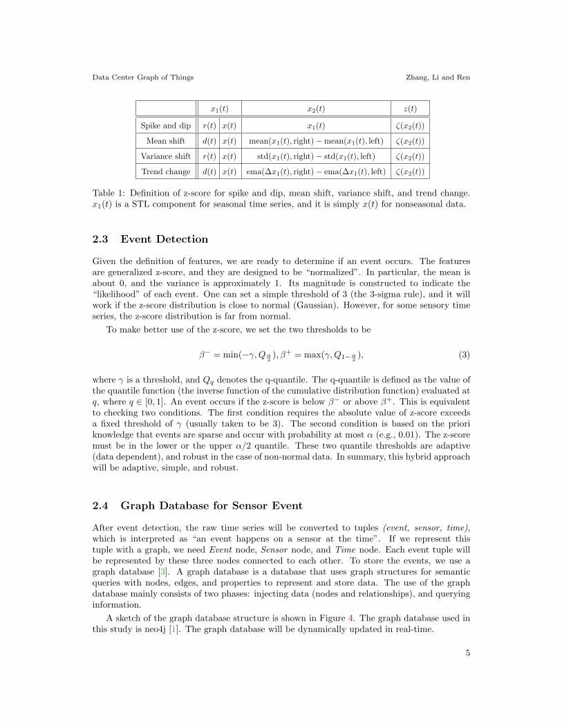
x1(t) x2(t) z(t)

Spike and dip r(t) x(t) x1(t) ζ(x2(t))

Mean shift d(t) x(t) mean(x1(t), right)−mean(x1(t), left) ζ(x2(t))

Variance shift r(t) x(t) std(x1(t), right)− std(x1(t), left) ζ(x2(t))

Trend change d(t) x(t) ema(∆x1(t), right)− ema(∆x1(t), left) ζ(x2(t))

Table 1: Definition of z-score for spike and dip, mean shift, variance shift, and trend change.x1(t) is a STL component for seasonal time series, and it is simply x(t) for nonseasonal data.

2.3 Event Detection

Given the definition of features, we are ready to determine if an event occurs. The featuresare generalized z-score, and they are designed to be “normalized”. In particular, the mean isabout 0, and the variance is approximately 1. Its magnitude is constructed to indicate the“likelihood” of each event. One can set a simple threshold of 3 (the 3-sigma rule), and it willwork if the z-score distribution is close to normal (Gaussian). However, for some sensory timeseries, the z-score distribution is far from normal.

To make better use of the z-score, we set the two thresholds to be

β− = min(−γ,Qα2

), β+ = max(γ,Q1−α2

), (3)

where γ is a threshold, and Qq denotes the q-quantile. The q-quantile is defined as the value ofthe quantile function (the inverse function of the cumulative distribution function) evaluated atq, where q ∈ [0, 1]. An event occurs if the z-score is below β− or above β+. This is equivalentto checking two conditions. The first condition requires the absolute value of z-score exceedsa fixed threshold of γ (usually taken to be 3). The second condition is based on the prioriknowledge that events are sparse and occur with probability at most α (e.g., 0.01). The z-scoremust be in the lower or the upper α/2 quantile. These two quantile thresholds are adaptive(data dependent), and robust in the case of non-normal data. In summary, this hybrid approachwill be adaptive, simple, and robust.

2.4 Graph Database for Sensor Event

After event detection, the raw time series will be converted to tuples (event, sensor, time),which is interpreted as “an event happens on a sensor at the time”. If we represent thistuple with a graph, we need Event node, Sensor node, and Time node. Each event tuple willbe represented by these three nodes connected to each other. To store the events, we use agraph database [3]. A graph database is a database that uses graph structures for semanticqueries with nodes, edges, and properties to represent and store data. The use of the graphdatabase mainly consists of two phases: injecting data (nodes and relationships), and queryinginformation.

A sketch of the graph database structure is shown in Figure 4. The graph database used inthis study is neo4j [1]. The graph database will be dynamically updated in real-time.

5


Figure 4: Structure of the graph database. There are three types of nodes: Event, Sensor,Time. Each event will be represented by three connected nodes (event, sensor, time). Eachnode has its own properties. For example, Event node contains event type, Sensor node storessensor information, and Time node has time stamp.

2.5 Sensor Connection

The next step will be querying this graph database and finding the connection between sensors.Intuitively, if two sensors have lots of events in common, they will have high connection weights.

A precise mathematical definition is needed to quantify this. Given a sensor i, denote allits event tuples within a given time window (say recent one month) as a set

Si = {(ek, tk)}, (4)

where ek, tk are the event type and event time respectively. k is the index of the events (k =1, 2, 3, · · · ). Consider two sensors (i, j), let their event set be Si = {(ek, tk)} and Sj = {(el, tl)}respectively. Fix a max time lag δ, and define the concurrent event set of j with respect to i asfollows:

S(i, j) = {(ek, tk) | ∃(el, tl), s.t., el = ek, |tl − tk| ≤ δ}. (5)

Next, denote the concurrent event count as C(i, j) = card(S(i, j)), where card(·) is the cardi-nality of a set. C(i, j) is the number of events of sensor i for which sensor j also has an eventof the same type at about the same time (max time difference δ). Intuitively, if C(i, j) is large,then sensor j has strong connection with sensor i.

Note that C(i, j) is not symmetric, i.e., C(i, j) 6= C(j, i) in general. Because the definitionis asymmetric: we are standing at the viewpoint of sensor i. By definition, C(i, i) = card(Si),i.e., the number of events of sensor i. Also, C(i, j) ≤ C(i, i), since C(i, j) only counts a subsetof Si.

The definition of concurrent count C(i, j) is not normalized, i.e., it has different magni-tudes for different sensors or different time windows. For a normalized measure, we define theprobability of a concurrent event of sensor j with respect to sensor i as

P (i, j) = C(i, j)/C(i, i), (6)

6


which is in the range [0, 1]. This quantity allows us to make meaningful comparison acrossdifferent times and sensors. Finally, to make the sensor connection measure symmetric, wedefine the connectivity as

A(i, j) = P (i, j)P (j, i), (7)

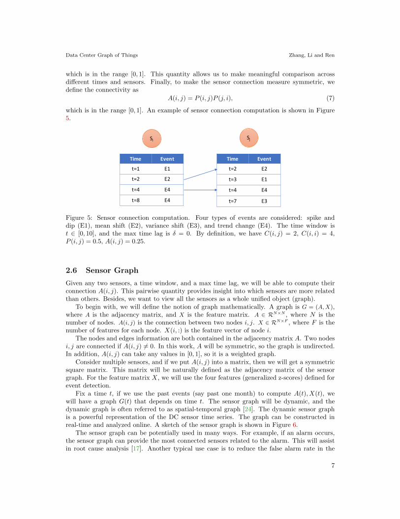
which is in the range [0, 1]. An example of sensor connection computation is shown in Figure5.

Time Event

t=1 E1

t=2 E2

t=4 E4

t=8 E4

Si Sj

Time Event

t=2 E2

t=3 E1

t=4 E4

t=7 E3

Figure 5: Sensor connection computation. Four types of events are considered: spike anddip (E1), mean shift (E2), variance shift (E3), and trend change (E4). The time window ist ∈ [0, 10], and the max time lag is δ = 0. By definition, we have C(i, j) = 2, C(i, i) = 4,P (i, j) = 0.5, A(i, j) = 0.25.

2.6 Sensor Graph

Given any two sensors, a time window, and a max time lag, we will be able to compute theirconnection A(i, j). This pairwise quantity provides insight into which sensors are more relatedthan others. Besides, we want to view all the sensors as a whole unified object (graph).

To begin with, we will define the notion of graph mathematically. A graph is G = (A,X),where A is the adjacency matrix, and X is the feature matrix. A ∈ RN×N , where N is thenumber of nodes. A(i, j) is the connection between two nodes i, j. X ∈ RN×F , where F is thenumber of features for each node. X(i, :) is the feature vector of node i.

The nodes and edges information are both contained in the adjacency matrix A. Two nodesi, j are connected if A(i, j) 6= 0. In this work, A will be symmetric, so the graph is undirected.In addition, A(i, j) can take any values in [0, 1], so it is a weighted graph.

Consider multiple sensors, and if we put A(i, j) into a matrix, then we will get a symmetricsquare matrix. This matrix will be naturally defined as the adjacency matrix of the sensorgraph. For the feature matrix X, we will use the four features (generalized z-scores) defined forevent detection.

Fix a time t, if we use the past events (say past one month) to compute A(t), X(t), wewill have a graph G(t) that depends on time t. The sensor graph will be dynamic, and thedynamic graph is often referred to as spatial-temporal graph [24]. The dynamic sensor graphis a powerful representation of the DC sensor time series. The graph can be constructed inreal-time and analyzed online. A sketch of the sensor graph is shown in Figure 6.

The sensor graph can be potentially used in many ways. For example, if an alarm occurs,the sensor graph can provide the most connected sensors related to the alarm. This will assistin root cause analysis [17]. Another typical use case is to reduce the false alarm rate in the

7


s1s2

s3

s4

s5

0.221.343.42

0.129.342.31

3.220.321.32

0.211.341.09

0.542.432.21

0.80.4

0.6

0.6

0.4

0.4

feature

Edge weight

Figure 6: A sketch of the spatial-temporal sensor graph G(t) at a particular time instant.

DC monitoring system. Current anomaly detection systems are mainly based on univariatetime series. A single sensor can be misleading and produces false alarms. For example, a singlesensor might have a sudden jitter (due to wrong reading) and will trigger a (false) alarm. Itis hard to tell if this is a false alarm by only looking at this single sensor. However, if thesensor graph is available, we can reference other related sensors. If all other related sensors arenormal, then it is possible to filter out this false alarm.

3 Graph of Things Prototype and Validation

This section demonstrates the use of the above ts2graph pipeline. We use real DC sensory datato build a DC graph of things (sensor graph). Next, we will validate this graph of things usingtwo priori knowledge.

3.1 Data Center Graph of Things Prototype

We use the sensory data for a data center building at Alibaba Cloud. The sensors include ITload, real-time power usage effectiveness (PUE), outside environment sensors (6 sensors), watercooling system sensors (25 sensors), hot aisle temperature sensors (58 sensors), and computerroom air conditioning (CRAC) unit fan speeds (72 sensors), for a total of 163 sensors. We followthe ts2graph pipeline, and construct the sensor graph. The time series measurement frequencyis five minutes. The recent one month data (May 12, 2018 to June 12, 2018) is used, and themax time lag is fifteen minutes.

A snapshot of the sensor graph is depicted in Figure 7. First of all, there are two clusters,and they correspond to hot aisles and CRACs. The cluster structures are consistent with ourpriori knowledge. This gives us confidence in ts2graph.

Also, we compare the adjacency matrix with the Pearson correlation matrix, as displayedin Figure 8. Pearson correlation matrix is computed from the same one month data, and wetake its absolute value. Each entry of the Pearson correlation matrix is defined as the Pearsoncorrelation coefficient between the two time series. It is visible that the adjacency matrix ismuch more “sparse”. The reason is that events are much more sparse in time and reveal thetrue behaviors of the sensors. However, the raw time series may contain lots of noise, andthe direct correlation coefficient may be misleading and indicates spurious correlations. Thischaracteristic is very appealing. A typical application will be finding out which sensors have a

8


Hot aisle

CRAC

Figure 7: A snapshot of the sensor graph. Nodes with high connections are closer, and edgelightness indicates connection magnitude. There are two clusters, and they correspond to hotaisles and CRACs.

strong connection with a target sensor. We can identify them by merely looking at a particularrow of the matrix. After sorting the connection weight in descending order, we then pick thetop connected sensors. Since the adjacency matrix is more “sparse”, we will be more confidentabout which sensor is related (or unrelated) to the target sensor.

Figure 8: Heatmap of the adjacency matrix (left) and Pearson correlation matrix (right). Theadjacency matrix is more “sparse”, in fact half of the values are less than 0.01.

9


3.2 Validation with Priori Knowledge

Given the constructed DC graph of things prototype, we want to validate further that it revealsmeaningful relationships. To verify the sensor graph, we must have some ground truth tocompare against. The ground truth could come from a priori knowledge. For example, supposethat we know two sensors are physically close to each other, and measure the same quantity(e.g., temperature). Then they should have high connection weight. The adjacency matrix ofthe sensor graph should support this fact. For validating the sensor graph (in particular theadjacency matrix), we will make use of two priori knowledge.

3.2.1 Related Outside Environment Sensors

First, the outside environment sensors include three types of sensors: temperature, humidity,and wet-bulb temperature (WBT). The technical definition of WBT [9] is unnecessary here,and can be simplified as: WBT is determined by both temperature and humidity. Besides,each of the three sensors has a redundant sensor. The redundant pair should have a veryhigh connection weight. In summary, these six sensors are strongly connected. This prioriknowledge is used as the ground truth. We design the following experiment to verify if theadjacency matrix (or correlation matrix) can recover these relationships:

1. pick a matrix (adjacency matrix or any of the three correlation matrices)

2. choose a target sensor from the six outside environment sensors and get its connection(with all other sensors) from the row of the matrix corresponding to that sensor

3. sort connection in descending order, and pick the top six related sensors

4. count the number of sensors in the top six list that comes from the six outside environmentsensors (the priori knowledge), divide by six, and call the result m1

5. sum up the connection weight of sensors that are in both the top six list and six outsideenvironment sensors list, divide by the total connection weight of target sensor (i.e., thesum of the matrix row), and denote this quantity as m2

6. sum up the connection weight of the six outside environment sensors, and divide by thetotal connection weight of the target sensor, let this number be m3

7. repeat step 2-6 and average m1,m2,m3 across all six sensors

The evaluation metric m1,m2,m3 are designed such that the higher, the better. For ex-ample, m1 is roughly the probability of recovering the top connected sensors (defined by thepriori knowledge) from the top connection list (encoded by the matrix). m2 measures the “con-fidence” when recovering the top connected sensors (the priori knowledge). m3 measures thetotal connection percentage of the top connected sensors (the priori knowledge). They are allnormalized to be in the range [0, 1].

For comparison, we also conduct the same experiment on the Pearson correlation matrix,Spearman rank correlation [21] matrix, and Kendall rank correlation [10] matrix. These threecorrelation matrices are all computed from the same one month data. Also, we take absolutevalue for the correlation matrices so that its value is in [0, 1]. Each entry of the correlationmatrix is defined as the correlation coefficient of the two time series. The experiment resultsare reported in Table 2. The adjacency matrix achieves the best result among all the matrices.Notice that m1 = 1.00 (100%) for the adjacency matrix, which means that the adjacency matrixalways finds the six related sensors (the priori knowledge) in its top six list (from the matrix).In terms of m2,m3, adjacency matrix outperforms correlation matrices by a factor of 2.

10


Adjacency Pearson Spearman Kendall

m1 1.00 0.77 0.77 0.75m2 0.35 0.14 0.13 0.15m3 0.35 0.15 0.13 0.15

Table 2: Evaluation metric for validation experiment based on six related outside environmentsensors. Adjacency matrix outperforms correlation matrices in terms of all evaluation metrics.

3.2.2 Related Temperature Sensors in Computer Room

Second, hot aisle temperature sensors from the same computer room should have strong con-nections (the priori knowledge). Because they are physically close to each other, and both aremeasuring the same physical quantity (temperature). There are seven computer rooms in theDC used in this work, each with eight hot aisle temperature sensors. Therefore, we can carryout a similar experiment as before. This time, we replace the top-six list by the top-eight list,and the priori knowledge of strongly connected sensors will be the sensors from the same com-puter room. The evaluation metric will be averaged for all hot aisle sensors. The results arereported in Table 3. Again, graph adjacency matrix beats correlation matrices for all metrics.For m2,m3 it outperforms by about 50%.

Adjacency Pearson Spearman Kendall

m1 0.46 0.43 0.45 0.46m2 0.16 0.06 0.09 0.11m3 0.22 0.11 0.14 0.15

Table 3: Evaluation metric for validation experiment based on related hot aisle temperaturesensors. Adjacency matrix achieves best performance in all evaluation metrics.

4 Graph of Things for Anomaly Detection

In the previous section, the sensor graph has been validated using two priori knowledge. In thissection, we will demonstrate the use of the sensor graph with anomaly detection.

4.1 Anomaly Detection Methods

4.1.1 Anomaly Detection

Data center (DC) is a complex system with lots of components, which includes IT devices andsupporting equipment. These components are interrelated, and they form the internet of things(IoT). Anomaly detection is crucial for the healthy running of DC.

Traditional anomaly detection mainly deals with time series, or vector inputs [5]. Recently,there have been some deep learning based anomaly detection methods [4]. However, the inputsof these algorithms are mainly vectors. These methods will work if the underlying data can bewell described by vectors.

However, in DC, IoT data sources are related in complex ways. The graph models both thefeatures of time series (node feature matrix) and their connections (adjacency matrix), whichmakes it a good candidate as the knowledge representation between DC sensors.

11


There have been some graph-based anomaly detection methods proposed in recent years[2]. However, these algorithms are still mainly based on conventional graph theory, such asthe shortest path and connected components. Though they process more information than thevector-based methods, those methods are still “shallow”. If the underlying graph data input hascomplex structures or hidden information, it will be hard for these methods to work effectively.

4.1.2 Graph Neural Network

To address this challenge, we can combine deep learning, graph as knowledge representation,and anomaly detection. Deep learning is able to discover hidden information and structurefrom data [12], and the input is usually a vector or image. Now the input is a graph. Thereforewe use deep learning for the graph, which is referred to as graph neural network (GNN) [2, 26].GNN extends the application domain of deep learning from vector or image to a graph. A graphis a versatile data structure with strong representation power. For example, an image can beviewed as a simple graph where each pixel is a node, and it is only connected to 8 nearby pixels.

Convolutional neural network (CNN) operates on image [11]. The most fundamental oper-ation of CNN is image convolution. In short, image convolution aggregates information fromnearby pixels for feature extraction [7].

GNN generalizes CNN to work on the graph [18]. The basic building block of GNN isgraph convolution, where the information of connected nodes is combined to extract featuresfor each node. The main difference from image convolution is that nearby pixels are replacedby connected nodes in the graph.

4.1.3 Methodology

To demonstrate the use of the sensor graph, we apply GNN to the sensor graph for the purposeof anomaly detection. In particular, we will apply the graph auto-encoder (GAE) [24]. Asbenchmark, we also consider conventional vector auto-encoder (VAE) [8] and principal compo-nent analysis (PCA) [15]. GAE compresses graph into hidden states (with lower dimension),and reconstructs it back. GAE is able to learn the hidden low dimensional structure in graphsdirectly. VAE learns the nonlinear low dimensional subspace on vector inputs. PCA works byfinding a linear subspace (of vectors) that best explains the variance in data.

Both these three methods fall into the category of subspace-based methods for anomalydetection [5]. Subspace based method assumes that most data are “normal” and lie in somelow dimensional subspace (linear or nonlinear). It tries to learn this subspace from data, thenproject data onto the subspace, and finally reconstruct the original input. “normal” data willhave small reconstruction error, but “anomaly” data will have a higher reconstruction error.Therefore, one can differentiate “anomaly” from “normal” based on the reconstruction error.

There exist many variants of graph convolution, as summarized in [24]. Some are based ongraph spectral theory, while others are spatially based. In this work, we define the followinggraph convolution operation:

Xk+1 = GCN(A,Xk) = UAXkW + B, (8)

where A ∈ RN×N is the adjacency matrix, Xk ∈ RN×Fk is the feature matrix at layer k. Nis the number of nodes, and Fk is the number of features for each node. A is the normalizedadjacency matrix, defined as A = D− 1

2AD− 12 , where D is a diagonal matrix of node degrees,

D(i, i) =∑

j A(i, j). U ∈ RN×N , W ∈ RFk×Fk+1are parameters, and B ∈ RN×Fk+1 is the bias.Notice that graph adjacency matrix is kept fixed across GCN layers, while the feature matrix

12


is transformed. The transformation of feature matrix depends on adjacency matrix, i.e., thetopology of the graph. After convolution, a tanh activation function is be applied.

The GAE used here consists of 3 layers. The first layer reduces the number of features pernode from 4 to 3, and applies the tanh activation. The second layer reconstructs the number offeatures from 3 to 4, followed by the tanh transformation. The third layer is a rescaling layer,where only graph convolution is applied, without activation function. The target output ofGAE is the original feature matrix, and backpropagation [8] is used to update the parameters.

For VAE and PCA, the input is the feature vector of the whole graph. The feature vectorof the whole graph is obtained by flattening the feature matrix X ∈ RN×4. As a result, thefeature vector has dimension R4N . VAE has the same three-layer structure as GAE, and thenumber of hidden states is equal to 3N . For PCA, we keep the top 3N principle componentsin the subspace, and reconstruction is based on 3N principal components. The characteristicsof the three described methods are summarized in Table 4.

Input Subspace Hidden state Output (target)

Graph auto-encoder (GAE) G = (A,X) Nonlinear Xh ∈ RN×3 G = (A,X)Vector auto-encoder (VAE) x = vec(X) Nonlinear xh ∈ R3N x = vec(X)

Principal component analysis (PCA) x = vec(X) Linear xh ∈ R3N x = vec(X)

Table 4: Summary of algorithms used. Both algorithms are replicating the input as the output.vec(X) denotes the flattened vector of a the feature matrix X.

4.2 Synthetic Anomaly Generation

The DC sensory data does not come with human expert anomaly labels. To circumvent thisissue, we choose to inject synthetic anomaly to the real data. In this work, we focus on theanomaly of a related group of sensors. Group anomaly is harder to detect and is of greater im-portance (corresponding to severe problems). For example, if the hot aisle temperature sensorsfrom the same computer room are experiencing rapid temperature increase simultaneously, thisis definitely an anomaly. In contrast, if a single sensor has a sudden short-time jitter (due tofalse reading), and all other related sensors stay the same, then this is probably not consideredan anomaly. It is very challenging for traditional time series based anomaly detection methodsto detect group anomaly. We consider two ways to generate synthetic anomaly. In the firstmethod, we modify the feature matrix directly. This is a necessary check for GNN to verifythat it works for anomaly graphs. In the second approach, we modify the original time seriesdirectly. This is more realistic because real anomaly originates from the raw time series.

4.2.1 Feature Matrix Anomaly

First, we add anomaly to the feature matrix of sensors directly. Note that the features (gen-eralized z-scores) are designed to be “normalized”, i.e., the mean is about 0 and variance isabout 1. At each time step, we set a 20% probability to modify the feature matrix. For eachmodification, we randomly choose a computer room (7 of them), and select the group of hotaisle temperature sensors from this computer room (8 sensors). Then we add (or subtract)random perturbation drawn from normal distribution N(3, 1) to the features corresponding tothese sensors. The anomaly label is set according to the affected sensors. Anomaly label willhave the same dimension as the number of sensors. The anomaly label is of “sensor” level,

13


i.e., it gives a label to each sensor. Of course, both feature matrix and anomaly label will bedependent on time. As a result, we have an anomaly label for each sensor at each time step.

4.2.2 Time Series Anomaly

A more realistic approach to generate anomaly is to modify the original time series directly. Asproposed, we care more about the anomaly of a related subgroup. To simulate this scenario,we design the following anomaly generation. At each time step, there is a 20% probability ofmodifying the time series. Then, we pick a computer room at random and find the group ofhot aisle temperature sensors in this computer room (8 sensors). For this sensor group, we addperturbation drawn from normal distribution N(6, 1) (unit: Celsius degree) to the next onehour time series. The anomaly label is assigned according to which sensor has an anomaly, andlasts for one hour. Therefore, the anomaly label is of “sensor” level and marks anomaly sensorfor each time step.

4.3 Experiment Result

In this section, we will show the result for two types of synthetic anomaly data. The trainingdataset contains four-week original clean data. The validation dataset contains one-week orig-inal data. The testing dataset contains one-week synthetic anomaly data. The measurementfrequency of the time series is five minutes.

4.3.1 Evaluation metric

As an anomaly detection task, we use precision, recall and F1-score [16] to evaluate the algo-rithm performance. Precision is defined as

precision =tp

tp + fp, (9)

where tp is the number of true positive, and fp is the number of false positive. Recall is definedas

recall =tp

tp + fn, (10)

where fn is the number of false negative cases. Intuitively, precision is the precision of ananomaly alarm (whether a predicted anomaly is an actual anomaly). Recall measures theability to find all anomalies (how many anomalies are found). F1-score combines precision andrecall into a single number, and is defined as the harmonic mean of precision and recall.

4.3.2 Evaluation Result

The anomaly score (“likelihood” of an anomaly) is based on the reconstruction error. Recon-struction error has the same dimension as the feature matrix, but we have a “sensor” levelanomaly label. Therefore, we will aggregate the reconstruction error by taking the averageacross four features for each sensor. The anomaly score is defined to be this “sensor” levelreconstruction error. Based on the anomaly score, one can obtain a precision (F1 score)-recallcurve by adjusting the threshold of anomaly prediction [5].

The results for the performance of graph auto-encoder (GAE), vector auto-encoder (VAE),and principal component analysis (PCA) are shown in Figure 9. For both datasets, GAEachieves the best performance, because it takes into account the topology relationship between

14


(a) Feature matrix anomaly (b) Time series anomaly

Figure 9: Precision (F1 score)-recall curve for anomaly detection on two synthetic dataset.GAE achieves the best preformance for both cases.

sensors. VAE outperforms PCA because the sensor relationship is nonlinear. For the firstdataset, GAE outperforms PCA by a factor of 3 to 4 in terms of both precision and F1 scorefor a wide range of recall ([0.2, 0.8]). In the second dataset, GAE gets twice precision (andF1 score) compared to VAE and PCA. Note that the time series anomaly dataset is morechallenging, as expected. For more realistic time series anomaly, VAE performance is no longerclose to GAE.

5 Conclusion

In this work, we propose ts2graph, a data-driven pipeline for constructing a DC graph of thingsbased on sensory time series. A prototype sensor graph (i.e., graph of things) is built witha real DC sensor time series dataset, and it is validated using two priori knowledge. Thesensor graph is capable of revealing meaningful relationships between sensors. To demonstratethe use of the sensor graph for anomaly detection, we evaluate the performance of the graphneural network. In particular, we apply graph auto-encoder (GAE) for anomaly detectionand compare against classical methods, including vector auto-encoder (VAE) and principalcomponent analysis (PCA). GAE stands out by a factor of 2 to 3 (in terms of precision andF1 score), because it takes into account the topology relationship between sensors. The sensorrelationships can not be captured by vector-based methods like VAE and PCA, and have to bedescribed by a graph. Based on this study, we expect the DC graph of things can serve as theinfrastructure for the DC monitoring system. DC graph of things will pave the way for bothanomaly detection and root cause analysis.

Acknowledgments

The authors kindly acknowledge Yue Li (Alibaba Group Inc) for helpful discussions about dataand proofreading the paper.

15


References

[1] Neo4j graph database. https://neo4j.com/. Accessed: 2020-02-20.

[2] Leman Akoglu, Hanghang Tong, and Danai Koutra. Graph based anomaly detection and descrip-tion: a survey. Data mining and knowledge discovery, 29(3):626–688, 2015.

[3] Renzo Angles and Claudio Gutierrez. Survey of graph database models. ACM Computing Surveys(CSUR), 40(1):1, 2008.

[4] Raghavendra Chalapathy and Sanjay Chawla. Deep learning for anomaly detection: A survey.arXiv preprint arXiv:1901.03407, 2019.

[5] Varun Chandola, Arindam Banerjee, and Vipin Kumar. Anomaly detection: A survey. ACMcomputing surveys (CSUR), 41(3):15, 2009.

[6] Robert B Cleveland, William S Cleveland, Jean E McRae, and Irma Terpenning. Stl: a seasonal-trend decomposition. Journal of official statistics, 6(1):3–73, 1990.

[7] Vincent Dumoulin and Francesco Visin. A guide to convolution arithmetic for deep learning. arXivpreprint arXiv:1603.07285, 2016.

[8] I Goodfellow, Y Bengio, and A Courville. Deep learning— the mit press. Cambridge, Mas-sachusetts, 2016.

[9] W Gupton Jr. HVAC controls: Operation and maintenance. Fairmont Press, 2001.

[10] Maurice G Kendall. A new measure of rank correlation. Biometrika, 30(1/2):81–93, 1938.

[11] Yann LeCun, Yoshua Bengio, et al. Convolutional networks for images, speech, and time series.The handbook of brain theory and neural networks, 3361(10):1995, 1995.

[12] Yann LeCun, Yoshua Bengio, and Geoffrey Hinton. Deep learning. nature, 521(7553):436, 2015.

[13] HB Mann. Non-parametric tests against trend. econometria. 1945. v. 13. pr, 246, 1945.

[14] Peter Mell, Tim Grance, et al. The nist definition of cloud computing. 2011.

[15] Karl Pearson. Liii. on lines and planes of closest fit to systems of points in space. The London,Edinburgh, and Dublin Philosophical Magazine and Journal of Science, 2(11):559–572, 1901.

[16] David Martin Powers. Evaluation: from precision, recall and f-measure to roc, informedness,markedness and correlation. 2011.

[17] James J Rooney and Lee N Vanden Heuvel. Root cause analysis for beginners. Quality progress,37(7):45–56, 2004.

[18] Franco Scarselli, Marco Gori, Ah Chung Tsoi, Markus Hagenbuchner, and Gabriele Monfardini.The graph neural network model. IEEE Transactions on Neural Networks, 20(1):61–80, 2008.

[19] Amit Singhal. Introducing the knowledge graph: things, not strings. Official google blog, 5, 2012.

[20] George W Snedecor and William G Cochran. Statistical methods, eight edition. Iowa stateUniversity press, Ames, Iowa, 1989.

[21] Charles Spearman. The proof and measurement of association between two things. Americanjournal of Psychology, 15(1):72–101, 1904.

[22] Gaurav Tripathi, Bhawna Sharma, and Sonali Rajvanshi. A combination of internet of things (iot)and graph database for future battlefield systems. In 2017 International Conference on Computing,Communication and Automation (ICCCA), pages 1252–1257. IEEE, 2017.

[23] Chengwei Wang, Krishnamurthy Viswanathan, Lakshminarayan Choudur, Vanish Talwar, WadeSatterfield, and Karsten Schwan. Statistical techniques for online anomaly detection in datacenters. In 12th IFIP/IEEE International Symposium on Integrated Network Management (IM2011) and Workshops, pages 385–392. IEEE, 2011.

[24] Zonghan Wu, Shirui Pan, Fengwen Chen, Guodong Long, Chengqi Zhang, and Philip S Yu. Acomprehensive survey on graph neural networks. arXiv preprint arXiv:1901.00596, 2019.

[25] Bing Yao, Xia Liu, Wan-jia Zhang, Xiang-en Chen, Xiao-min Zhang, Ming Yao, and Zheng-xueZhao. Applying graph theory to the internet of things. In 2013 IEEE 10th International Conference

16

https://neo4j.com/


on High Performance Computing and Communications & 2013 IEEE International Conference onEmbedded and Ubiquitous Computing, pages 2354–2361. IEEE, 2013.

[26] Jie Zhou, Ganqu Cui, Zhengyan Zhang, Cheng Yang, Zhiyuan Liu, and Maosong Sun. Graphneural networks: A review of methods and applications. arXiv preprint arXiv:1812.08434, 2018.

17

alibaba group inc. 500 108th ave ne suite 800, bellevue

Documents