alkali-based displacement processes in microfluidic ...in this thesis, alkaline flooding was...

Background and Context i

Alkali-based Displacement Processes in Microfluidic Experiments: Advanced Statistical Analyses

Ahmad Kharrat Master Thesis 2018 supervised by: Univ.-Prof. Dipl.-Phys. Dr.habil. Holger Ott

Background and Context iii

To my lovely wife Negin and my beloved parents

Background and Context v

Declaration

I hereby declare that except where specific reference is made to the work of others, the contents

of this dissertation are original and have not been published elsewhere. This dissertation is the

outcome of my own work using only cited literature.

Erklärung

Hiermit erkläre ich, dass der Inhalt dieser Dissertation, sofern nicht ausdrücklich auf die Arbeit

Dritter Bezug genommen wird, ursprünglich ist und nicht an anderer Stelle veröffentlicht

wurde. Diese Dissertation ist das Ergebnis meiner eigenen Arbeit mit nur zitierter Literatur.

____________________________________

Name, 23 September 2018

Background and Context vii

Acknowledgements

I would first like to express my deep gratitude to my supervisor Prof. Holger Ott for his creative

ideas, immense knowledge, thoughtful feedback and continuous support, which he has given

me since the very beginning.

I would also like to thank my collogues Pit Arnold, Mostafa Borji, Neda Hassannayebi and

Michael Koopmans for their guidance and support.

A loving thanks to my parents, especially my father, Prof. Riyaz Kharrat for unfailing

supported, patience and continuous encouragement through my years of study.

To my wife Negin, thank you for your admirable love, rock-solid support and patience during

my study.

Background and Context ix

Abstract

Since oil production declines over time, waterflooding and Enhanced Oil Recovery (EOR) are

applied to increase the recovery, at the secondary and tertiary stages of production.

Waterflooding is used for pressure maintenance and oil displacement, while the injection of

chemically modified water may lead to a higher recovery in the tertiary stage of production.

Water-based EOR methods, such as alkaline, surfactant and/or polymer flooding are commonly

used due to their efficiency and low cost. Especially attractive is alkaline flooding, in which oil

displacement is enhanced through interfacial tension (IFT) reduction, microemulsion

generation and wettability alteration.

In this thesis, alkaline flooding was investigated by using microfluidics (2D porous media

etched in glass) providing (a) a well-defined chemical environment and (b) displacements can

be studied with high spatial and time resolutions. Hence, microfluidics allows studying

chemical EOR processes in great detail.

In the frame of the present study, several experiments have been performed with different water

compositions varying the alkalinity and salinity of the injection water. All the experiments were

performed with crude oil of target field from Vienna basin, which has a high viscosity and TAN

number. The flooding experiments have been performed in different porous media, representing

high and low permeability and capillarity systems.

The purpose of this work was to enhance the experimental workflow in order to eliminate earlier

observed inconsistencies. In this frame, it turned out that conventional measurements like the

oil production from the porous medium (recovery) are not a good measurement, because the

flooding domain does not represent an elementary volume for multi-phase flow.

Therefore, discrete frequency distribution and Lorenz plot analyses were applied to characterize

the efficiency of water flooding and EOR process by acquiring quantities of data for comparing

the results and understanding complex displacements.

Based on the obtained results, the synthetic water performed like an alkali agent and displaced

a significant amount of oil compared to the pure-water flood. Upon statistical analyses, it has

been observed that oil cluster size was reduced in alkaline flooding, which can be used as a

fingerprint that distinguishes this process from water flooding. However, the link and

connection between statistical analyses with ultimate recovery were not achieved and still

requires further investigation.

Background and Context xi

Zusammenfassung

Da die Menge an produziertem Öl mit der Zeit abnimmt, werden sekundäre und tertiäre

Methoden, wie Wasserflutungen und Enhanced Oil Recovery (EOR), angewendet.

Wasserflutungen werden zur Druckerhaltung und Verdrängung von Öl angewendet,

wohingegen das Verpressen von chemisch modifiziertem Wasser im tertiären Stadium der

Produktion zu einer höheren Ölgewinnung führt. Auf Wasser basierende EOR Methoden, wie

Alkali-, Tensid- und/oder Polymerflutungen werden häufig verwendet, da sie kostengünstig

und effizient sind. Besonders reizvoll sind dabei Alkaliflutungen, bei welchen die Menge an

verdrängtem Öl durch die Reduzierung der Grenzflächenspannung, Bildung von

Mikroemulsionen und Veränderung der Oberflächenbenetzung erhöht wird.

In dieser Arbeit wurden Alkaliflutungen mit Hilfe der Mikrofluidik (2D poröse Medien in Glas

geätzt) untersucht, welche (a) eine chemisch gut definierte Umgebung liefern und (b)

Verdrängungsprozesse können mit hoher räumlicher und zeitlicher Auflösung erforscht

werden. Daher ermöglicht die Mikrofluidik die ausführliche Untersuchung chemischer EOR

Prozesse.

Im Rahmen dieser Arbeit wurden mehrere Experimente mit Wässern unterschiedlicher

Zusammensetzungen, welche sich in Alkalität und Salinität unterscheiden, durchgeführt. Alle

Experimente wurden mit Rohöl vom Wiener Becken durchgeführt, welches eine hohe

Viskosität und Gesamtsäurezahl hat. Die Flutungsexperimente wurden in verschiedenen

porösen Medien, welche Systeme mit hoher und niedriger Durchlässigkeit und Kapillarität

repräsentieren.

Das Ziel dieser Diplomarbeit war die Verbesserung der experimentellen Arbeitsabläufe um

zuvor beobachtet Unbeständigkeiten beheben. In diesem Rahmen hat sich herausgestellt, dass

konventionelle Messungen, wie die Öl Produktion von einem porösen Medium keine gute

Messung ist, da der geflutete Bereich kein repräsentatives elementares Volumen für

Mehrphasenströmung ist.

Daher wurden diskrete Häufigkeitsverteilungen und Lorenz Diagramm Analysen angewendet,

um die Effizienz der Wasserflutungs- und EOR Prozesse durch Aneignung von Datenmengen

zum Vergleichen der Ergebnisse, sowie dem Verstehen der komplexen Verdrängungsprozesse,

zu charakterisieren.

Aufbauend auf den erlangten Resultaten, verhält sich synthetisches Wasser wie ein Alkalimittel

und verdrängt einen bedeutenden Anteil an Öl verglichen mit einer reinen Wasserflutung.

Durch statistische Analysen wurde festgestellt, dass Ölgruppengrößen in alkalischen Flutungen

reduziert wurden, was als Leitparameter zur Unterscheidung dieser Prozesse von

Wasserflutungen genutzt werden kann. Jedoch konnte keine Verbindung zwischen den

statistischen Analysen und der Gesamtproduktion von Öl hergestellt werden, weshalb noch

weitere Untersuchungen vonnöten sind.

Table of Contents

Declaration ................................................................................................................................. v Erklärung ................................................................................................................................... v Acknowledgements .................................................................................................................. vii Abstract ..................................................................................................................................... ix Zusammenfassung..................................................................................................................... xi Chapter 1 .................................................................................................................................... 1 Introduction ................................................................................................................................ 1

1.1 Background and Context ............................................................................................ 2 1.2 Scope and Objectives ................................................................................................. 2

Chapter 2 .................................................................................................................................... 3 Literature Review....................................................................................................................... 3

2.1 Oil recovery and EOR ................................................................................................ 3 2.2 Alkaline Flooding ...................................................................................................... 3 2.3 Capillary Desaturation curve ..................................................................................... 6 2.4 Microfluidics .............................................................................................................. 8 2.5 Displacement process in pore scale ........................................................................... 9

Chapter 3 .................................................................................................................................. 11 Experimental Equipment ......................................................................................................... 13

3.1 Injection and Vacuum material ................................................................................ 13 3.2 Micromodel and Chip holder ................................................................................... 15 3.3 The Microscope ....................................................................................................... 16

Chapter 4 .................................................................................................................................. 19 Experimental methodology ...................................................................................................... 19

4.1 Alkaline Flooding Methodology .............................................................................. 19 4.2 Image Acquisition .................................................................................................... 23 4.3 Image Analyses ........................................................................................................ 25 4.4 Discrete frequency distribution analysis .................................................................. 27 4.5 Lorenz curve analysis .............................................................................................. 29

Chapter 5 .................................................................................................................................. 31 Results and Discussion ............................................................................................................ 31

5.1 Ultimate Recovery factor results.............................................................................. 31 5.2 Advance Statistical analyses .................................................................................... 36 5.3 Capillary Desaturation curve ................................................................................... 69

Chapter 6 .................................................................................................................................. 71 Conclusion ............................................................................................................................... 71

6.1 Summary .................................................................................................................. 71 6.2 Future Work ............................................................................................................. 72

Chapter 7 .................................................................................................................................. 73 References ................................................................................................................................ 73

List of Figures

Figure 2-1- Schematic picture of alkali process (E.F. deZabala, 1982) ..................................... 4 Figure 2-2- Schematic CDC (Larry W. Lake, 2014) ................................................................. 7 Figure 2-3- Micromodel from Micronit company, white color shows the flowing channels .... 9 Figure 2-4- Phase diagram of displacement patterns (Y. Alzahid, P. MOstaghimi, M. Ebrahimi Warkiani, R T. Armstrong, 2017) ............................................................................................ 10 Figure 2-5- Displacement patterns and the transition zone between them (Yi‐Feng Chen, Shu Fang, Dong‐Sheng Wu, Ran Hu, 2017) ................................................................................... 11 Figure 2-6- Displacement patterns observation based on capillary and mobility number in fractured micromodel (Yi‐Feng Chen, Shu Fang, Dong‐Sheng Wu, Ran Hu, 2017) .............. 11 Figure 3-1- Experiment setup .................................................................................................. 13 Figure 3-2- NE-300 syringe pump ........................................................................................... 14 Figure 3-3- Syringe (Left, glass syringe, right- Plastic syringe) .............................................. 14 Figure 3-4- Vindum VP-12K continuous pulse-free high-pressure metering pump ................ 15 Figure 3-5- Vacuum pump ....................................................................................................... 15 Figure 3-6- Physical rock micromodel in left and High-Pressure chip holder in right (Micronit, 2018) ........................................................................................................................................ 16 Figure 3-7- DMi 8 Leica microscope (www.leica-microsystems.com) ................................... 17 Figure 4-1- Cleaned micromodel ............................................................................................. 20 Figure 4-2- 100% oil-saturated micromodel ............................................................................ 20 Figure 4-3- Micromodel after water flooding, dark areas correspond to remaining oil at the end of the water flood ..................................................................................................................... 21 Figure 4-4- The final stage of alkaline flooding (Sodium hydroxide), dark areas correspond to remaining oil at the end of the alkaline flooding. .................................................................... 21 Figure 4-5- Individual (lower row) and stitched images for a) the physical rock pattern, and b) the uniform pattern. .................................................................................................................. 24 Figure 4-6- Binarizing physical rock micromodel in ImageJ, a) raw image, b) binarized picture ................................................................................................................................................. 25 Figure 4-7- Cluster length and area for one individual cluster ................................................ 27 Figure 4-8- Objects map of experiment 1.1 ............................................................................. 27 Figure 4-9- Cluster analysis overview (Ott, 2018) .................................................................. 28 Figure 4-10- Frequency and cluster volume sizes distribution of experiment 1 ...................... 28 Figure 4-11- Normal distribution of distilled WF with 0.01 ml/h ........................................... 29 Figure 4-12- Lorenz plot of experiment 1.1 ............................................................................. 30 Figure 5-1- Remaining oil recovery in tertiary flooding for, a) Solution with distilled water, b) Solution with synthetic water, c) 720 ppm NaOH with different injection rate, d) in Physical rock with 0.001 ml/h injection rate, e) in Uniform with 0.001 ml/h ........................................ 35 Figure 5-2- Binary Image of a) distilled water flooding (experiment 2.1), b) synthetic water flooding (experiment 6.1) after 22 hours, c) synthetic water flooding (experiment 6.1) after 62 hours......................................................................................................................................... 38 Figure 5-3-a) Tile picture crude oi1 and distilled water, b) IFT measurement of distilled water and crude oil with the spinning drop (Arnold, 2018) ............................................................... 39 Figure 5-4-a) Tile picture crude oi1 and synthetic water, b) IFT measurement of synthetic water and crude oil with the spinning drop (Arnold, 2018) ............................................................... 39 Figure 5-5- The final stage of all the water flooding with 0.01 ml/h ....................................... 39 Figure 5-6- Statistical analyses for waterflooding with 0.01 ml/h, a) cluster size distribution, b) Normalize distribution c) b) Lorenz plot ............................................................................. 41 Figure 5-7- Oil entering micromodel during waterflooding, time steps is from left to right ... 41 Figure 5-8- Statistical analyses for Distilled waterflooding with 0.01 ml/h, a) cluster size distribution, b) Normalize distribution, c) Lorenz plot ............................................................ 43 Figure 5-9- Comparison of water flooding with Lorenz plot ................................................... 43

Figure 5-10- The last stage of water flooding for a) Exp 1.1 (this thesis), b) Exp 1.1.1 (Borji, 2017) ........................................................................................................................................ 44 Figure 5-11- Statistical analyses for 3000 ppm Na2CO3 a) cluster size distribution for AF, b) cluster size distribution for WF and AF, c) Normalize distribution, d) Lorenz plot ................ 46 Figure 5-12- Last stage of 3000 ppm flooding Na2CO3, a) Exp 1.1.1, b) Exp 2.1.1 ................ 46 Figure 5-13- Last stage of 7500 ppm Na2CO3 flooding a) Exp 3.1.1, b) Exp 4.1.1 ............... 47 Figure 5-14- Statistical analyses for 7500 ppm Na2CO3 a) cluster size distribution for AF, b) cluster size distribution for WF and AF, c) Normalize distribution, d) Lorenz plot ................ 49 Figure 5-15- Synthetic flooding a) Experiment 5.1, b) Experiment 5.1.1, c) Experiment 6.1 d) Experiment 6.1.1 ...................................................................................................................... 49 Figure 5-16- Statistical analyses for synthetic WF and AF, a) cluster size distribution for WF and AF, b) Normalize distribution, c) Lorenz plot................................................................... 51 Figure 5-17- Process images of the final stage, a) Exp 2.1.1 (3000 ppm Na2CO3), b) Exp 4.1.1 (7500 ppm Na2CO3), c) Exp 7.1.1 (720 ppm NaOH) .............................................................. 52 Figure 5-18- Pinned clusters due to microemulsion in 7500 ppm Na2CO3 in different pore volume ..................................................................................................................................... 53 Figure 5-19- Microemulsion generation in 7500 ppm Na2CO3 flooding in different pore volume ................................................................................................................................................. 53 Figure 5-20- Images of droplets in micromodel and spinning drop of Na2CO3 a)3000 ppm, b) 7500 ppm ................................................................................................................................. 54 Figure 5-21- Statistical analyses for all flooding with 0.01 ml/h, a) cluster size distribution for WF and AF, b) Normalize distribution, c) Lorenz plot............................................................ 56 Figure 5-22- Last stage of flooding a) water, b) 720 ppm NaOH flooding ............................. 57 Figure 5-23- Statistical analyses for NaOH with different injection rate, a) cluster size distribution for WF and AF, b) Normalize distribution, c) Lorenz plot ................................... 59 Figure 5-24- Last stage of experiment 12.1.1 (6000 ppm Na2CO3) ......................................... 60 Figure 5-25- Microemulsion in experiment 12.1.1 (6000 ppm Na2CO3) ................................. 60 Figure 5-26- Statistical analyses for 6000 ppm Na2CO3 and 720 ppm NaOH, a) cluster size distribution for WF and AF, b) Normalize distribution, c) Lorenz plot ................................... 62 Figure 5-27- Statistical analyses for microemulsion generation, a) cluster size distribution for AF, b) Normalize distribution, c) Lorenz plot ......................................................................... 63 Figure 5-28- Secondary drainage in the uniform pattern ......................................................... 64 Figure 5-29- Binary image at the final stage of a) Experiment 10.1, b) Experiment 11.1, c) Experiment 13.1 ....................................................................................................................... 65 Figure 5-30- Binary image at the final stage of a) Experiment 10.1.1(720 ppm NaOH), b) Experiment 11.1.1(950 ppm Na2CO3), c) Experiment 13.1.1(6000 ppm Na2CO3) ................. 66 Figure 5-31- Statistical analyses for the uniform pattern, a) cluster size distribution for WF and AF, b) Normalize distribution, c) Lorenz plot .............................................................. 68 Figure 5-32- Flow pattern for a) Uniform, b) Physical rock .................................................... 68 Figure 5-33- Capillary desaturation curve for the experiments ............................................... 69

List of Tables

Table 3-1- Micromodels specification (Micronit, 2018) ......................................................... 16 Table 3-2- Field of view for microscope objectives ................................................................ 17 Table 4-1- IFT measurement at 25°C (Arnold, 2018) ............................................................. 22 Table 4-2- Experiments details ................................................................................................ 23 Table 5-1- Recovery factor for physical rock pattern with 0.01 ml/h ...................................... 32 Table 5-2- Recovery factor for physical rock pattern with 0.001 ml/h .................................... 32 Table 5-3- Recovery factor for the uniform pattern with 0.001 ml/hr. .................................... 33

Nomenclature

T temperature [c]

Viscosity

Capillary number

u

Q

Abbreviations

EOR Enhanced oil recovery

CDC Capillary desaturation curve

IFT Interfacial tension

WF Water flooding

AF Alkaline flooding

RF Recovery factor

REV Representative elementary volume

Chapter 1

Introduction It is anticipated that the global energy demand will increase by around 35% from 2011 to 2035.

Fossil fuels will be the focal source of energy and their share in the world’s energy supply is

expected to be around 80% in 2035 (International Energy Agency, 2013).

Hydrocarbon recovery operations consist of three phases. At first, oil is produced by natural

depletion (primary recovery), while water or gas is generally injected subsequently (secondary

recovery). If the reservoir is considered depleted by conventional means, enhanced oil recovery

(EOR) techniques may be applied (tertiary recovery). Most oil reservoirs are candidates for

enhanced oil recovery (EOR), while significant quantities of oil remain in place after applying

traditional methods. Based on the published literature, there are many different EOR methods,

which have been implemented and evaluated by the industry and academia. It is obvious that

no single recovery method will apply to all reservoirs. Therefore, it is necessary to choose the

best method for any given set of conditions, which is called EOR screening. EOR techniques

are increasingly being considered to satisfy the growing demand of oil in future. In fact, it has

been suggested that 88 billion barrels of oil will produce additionally, by increasing 1% of oil

recovery factor, at current rates (Sheng, 2013). Chemical flooding may be applied in tertiary

oil recovery by adding polymers, alkaline, and surfactants to the injection water, which helps

the mobilization of the trapped oil in the reservoir rock by decreasing the interfacial tension, by

altering wettability, and by enhancing water viscosity (S. Kokal, 2010). This could be achieved

through single or multiple changes in reservoir fluids properties and its interfacial energy (Lake,

1989). Alkaline flooding is one of the earliest-applied and cheapest methods amongst chemical

flooding methods. The primary mechanisms are the reduction of interfacial tension, the

resulting microemulsion generation and a change in wettability.

In the frame of this thesis, alkaline flooding is investigated by using microfluidics (2D porous

media etched in glass)

2 Background and Context

1.1 Background and Context Alkaline flooding was first performed in the 20th century. However, few works have been

reported in alkaline flooding recently. (Borji, 2017) and (Arnold, 2018) achieved significant

results on alkaline flooding on the pore scale using microfluidics and on fluid-fluid interfacial

properties, respectively. The present thesis is following the earlier work and applied similar

techniques to obtain a better understanding of the processes by investigating their fingerprints.

1.2 Scope and Objectives In this work, fluid displacements are investigated on the pore scale for different injection-water

solutions with different alkalinity. Furthermore, displacements have been studied in two

different microfluidic devices, representing low and high capillarity systems.

One of the objectives is to achieve repeatable and reproducible results in the experiments.

Moreover, by applying statistical analyses, we found quantitative signatures of water and

alkaline flooding processes, and a relationship between statistical analyses and ultimate

recovery factor.

Chapter 2

Literature Review This chapter describes the basic principle and gives a brief introduction to oil recovery and their

mechanism on the macroscopic and microscopic scale.

2.1 Oil recovery and EOR The hydrocarbon production from underground history dates back to the 18th century. From

then, different operations were used to increase the hydrocarbon recovery, which is divided into

primary, secondary, tertiary (EOR) recovery methods. Upon the increase of the oil price, EOR

becomes more demanding, while the recovered oil form most of the reservoirs is less than 50 %

without EOR. There is a different type of EOR classification methods such as conventional and

unconventional (Riyaz Kharrat, 2017) or chemical, thermal, solvent and other (Larry W. Lake,

2014). The main mechanism of chemical EOR is to increase the capillary number to mobilize

remaining oil and to control the mobility to increase the sweep efficiency (Hu Guo, Ma Dou,

Wang Hanqing, Fuyong Wang, Gu Yuanyuan, Zhaoyan Yu, Wang Yansheng, Yiqiang Li,

2017). The main focus of this thesis is on alkaline flooding.

2.2 Alkaline Flooding In 1917 Squires, the first-time added alkali to the injection water, and observed that oil

displacement improved (Squires, 1917). This method is one of the cheapest, which is still used

(E.F. deZabala, 1982). Based on the literature, Alkaline flooding has been used in 36 projects

and six different countries (Sheng, 2015).

4 Alkaline Flooding

2.2.1 Alkaline reaction with oil The reaction between an acid component of the oil and alkali agents leads to soap generation

at the oil and water interface (C. E. Cooke, 1974). Figure 2-1 shows a schematic view of this

process.

Figure 2-1- Schematic picture of alkali process (E.F. deZabala, 1982)

To understand the saponification, a number of chemical reactions need to be considered. The

dissociation reaction of sodium hydroxide in water is shown in equation (2-1) and the reaction

of sodium hydroxide with an acid oil component is illustrated in Equation (2-2), where HA

represents the acid component of oil.

(2-1)

(2-2)

Equation (2-3) and (2-4) show the sodium carbonate dissociation and formation of carbonic

acid. Additionally, equation (2-5) describes the reaction of oil acid component.

(2-3)

(2-4)

(2-5)

Both alkali agents were used in this thesis.

Alkaline Flooding 5

Alkaline flooding performance is mainly depending on crude oil and water composition, rock

reactivity and alkaline concentration and slug size (Johnson, 1976). Up to this point, eight

different mechanisms are known for this EOR method, which are shown in the following (E.F.

deZabala, 1982):

Emulsification with entrainment

Emulsification with entrapment

Emulsification with coalescence

Wettability reversal

Wettability gradients

Oil-phase swelling

Disruption of rigid films

Reducing interfacial tensions

Some of these mechanisms have been observed by Borji (Borji, 2017) and in the frame of this

thesis.

Reduction of IFT

In alkaline flooding, the IFT reduction results from the in-situ generated soap which is forming

of reaction between an acid oil and an alkali solution (C. E. Cooke Jr., R. E. Williams, P. A.

Kolodzie, 1974). Moreover, Capillary force is also decreased as a result of IFT reduction, which

is discussed further below in the context of the Capillary Desaturation curve.

Emulsification

If the IFT reduced significantly, the mixture of oil and water may lead to emulsion formation.

Emulsification is mainly divided to entrainment and entrapment

Emulsification and entrainment

The oil emulsifies in water due to IFT reduction and displaced within the aqueous phase

(Subkow, 1942). Therefore, the displacement efficiency improved which leads to higher oil

recovery.

Emulsification and entrapment

If the size of emulsified oil clusters is larger than the pore throat sizes, the flowing paths will

block by the emulsion. Therefore, the fluid flows through unswept pores and the sweep

efficiency increases. However, this mechanism is only observed in heavy viscous oil with a

high TAN number (Ehrlich R., Hasiba H.H., Raimondi P., 1974).

6 Capillary Desaturation curve

Wettability reversal

Depend on the initial condition, the change from oil-wet to water-wet may occur or the reverse.

When an oil-wet system changed to a water-wet, the relative permeabilities also change in

favourable direction and leads to oil recovery improvement. Thought, changing the water-wet

to oil-wet reservoir results to connecting the discontinuous residual oil phases and providing

the flow path for trapped oil. Additionally, oil-external emulsions of water droplets block the

flow and induce a high-pressure gradient, which can overcome the capillary force (Sheng,

2011).

2.3 Capillary Desaturation curve To describe the impact of alkaline flooding on residual oil in the reservoir the capillary

desaturation curve (CDC) is used. CDC is one of the fundamental concepts in enhanced oil

recovery and describes the relationship between residual saturation of wetting and non-wetting

fluid phase with the capillary number (Nc). This number is the ratio of viscous forces to capillary

forces and is defined in equation (2-6), where and u are the viscosity and interstitial velocity

of the displacing fluid or wetting phase, respectively, and is the interfacial tension between

two fluids (Larry W. Lake, 2014). The nonwetting saturation is constant at plateau value, when

the capillary number is small. The reduction of nonwetting saturation starts at critical capillary

number. This number is achieved either by increasing the viscous force or reducing the capillary

force.

Nc (2-6)

Figure 2-2 shows a schematic CDC, where the X-axis denotes the capillary number and Y-axis

denotes the residual nonwetting or wetting residual phase saturation. The critical capillary

number, above which desaturation occurs is about Nc ~ 10-5 to 10-7 depending on the wetting

state of the sample (Dullien, 1979).

Capillary Desaturation curve 7

Figure 2-2- Schematic CDC (Larry W. Lake, 2014)

In 1974, Melrose and brander proposed new capillary number (macro capillary number) by

applying the Darcy law into the equation. They stated that by achieving the IFT value in the

order of 10-3 to 10-4 dynes/cm, the residual oil saturation would be reduced (J. C. Melrose, C.

F. Brandner, 1974). Later on, Hilfer and Øren (A. Lucian, R. Hilfer, 1999) proposed a new

equation for macro capillary number based on connecting and upscaling the microscopic and

macroscopic images. In 2014, Armstrong, Georgiadis, and Ott modified the Lucian and Hilfer

model and defined a new equation (2-7), where is the cluster length in the flow direction,

is wetting phase viscosity, is Darcy velocity, is relative permeability of wetting

phase and is capillary pressure. The average value of these parameters is measured from the

X-ray computed microtomography and transformed from micro (pore scale) to macro scale.

Moreover, they observed the nonwetting phase mobilization at Ncmacro ~ 1 (Ryan T. Armstrong,

Apostolos Georgiadis, Holger Ott, Denis Klemin, Steffen Berg, 2014)

Ncmacro (2-7)

Yegane and Hegner simplified the capillary number by applying the flow rate and Darcy law

in the equation and proposed that the critical oil ganglia lengths have an inverse relation with

the capillary number and it depends on rock properties such as porosity and permeability.

(Mohsen Yeganeh, Jessica Hegner, Eric Lewandowski, Aruna Mohan, Larry W. Lake, Dan

8 Microfluidics

Cherney, Arben Jusufi, Aditya Jaishankar , 2016). Equation (2-8) shows the capillary number,

where the Q is the flow rate, A is the area and is the porosity.

Ncmicro (2-8)

2.4 Microfluidics The displacement processes can be studied with high spatial and time resolutions in

microfluidics devices. Micromodels are simplified porous network, which may represent a rock

structure, or any other porous medium. It is essentially a 2D pore structure etched in glass (in

this thesis), with the structure being covered by another glass plate. Microfluidic experiments

were first performed by Chatenever and Calhoun in 1952. Their model was developed to study

fluid flow in porous media (A. Chatenever, J. Calhoun, 1952). Later, the cover glass was etched

chemically with hydrofluoric acid in order to create networks (C. Mattax, J.R. Kyte, 1962).

Since then, microfluidics has extensively been used to study two-phase flow and displacement

mechanisms. A famous example is the study by Lenormand investigating displacement stability

and the structure of the resulting displacement patterns (Roland Lenormand, Cesar Zarcone,

1985)

Micromodels are manufactured from transparent materials such as glass or polymer-based

materials, which are cheaper compared to glass (Shao-Yiu Hsu, Zhong-Yao Zhang, Chia-Wen

Tsao, 2017). Nowadays, the complex porous media can be manufactured with a high degree of

details by using laser technology (N. K. Karadimitriou and S. M. Hassanizadeh, 2012).

The use of microfluidics is well established to examine the microscopic behavior of multiphase

flow in porous media. It gives a significant advantage to see the movement of fluid interfaces

and makes it possible to distinguish between different kinds of mechanisms that may all lead

to similar production behavior. The size and depth of the pore structure are adjustable and may

serve different objectives of the experiment. Figure 2-3 shows a pore structure with a rather

random distribution of grains as it has been used in this thesis. The white color describes the

pore space and flowing path, while the grains are shown with black color in the micromodel.

The dimensions of the porous domain are 2 cm in length, 1 cm width and 20 microns etching

depth.

Displacement process in pore scale 9

Figure 2-3- Micromodel from Micronit company, white color shows the flowing channels

2.5 Displacement process in pore scale Two phase immiscible displacements are a complex process and especially rich on the pore

scale. This can best be illustrated by the work of Lenormand; he observed several fundamentally

different displacement patterns on the pore-scale. The displacements could be characterized by

viscous and capillary fingering and stable displacement as a function of the mobility and

capillary number (R. Lenormand, 1990). It should be mentioned that mobility number was

defined as the ratio of viscosity of the displacing fluid to the displaced fluid. Moreover, viscous

fingering occurs mainly when the displacing fluid has a lower viscosity compared to the

displaced fluid. The invasion-percolation theory describes the capillary fingering, where the

fluids flow in pore throats will lower capillary forces (Christophe Cottin, Hugues Bodiguel,

Annie Colin, 2010). Additionally, the stable displacement achieved by increasing the viscous

forces. This also is shown as phase diagram in Figure 2-4. The graph is double log scale, where

X-axis is logarithm of mobility number (Ratio of displacing fluid to displaced fluid) and Y-axis

is logarithm of capillary number (Y. Alzahid, P. MOstaghimi, M. Ebrahimi Warkiani, R T.

Armstrong, 2017).

10 Displacement process in pore scale

Figure 2-4- Phase diagram of displacement patterns (Y. Alzahid, P. MOstaghimi, M. Ebrahimi

Warkiani, R T. Armstrong, 2017)

In term of capillary and mobility number, the stable displacement occurs, where the mobility

and capillary numbers are close to one. While viscous fingering is occurring with high mobility

and low capillary numbers. In contrast, the capillary fingering occurs with low mobility and

high capillary numbers. The experimental observation of the displacement and transition and

crossover zone between these displacements are shown in Figure 2-5. The blue color illustrated

the transition zone between capillary to viscous fingering. The experimental observation is

shown in Figure 2-6, where ‘y’, ‘z’, ‘z1’ and ‘z2’ demonstrate the capillary fingering and ‘a-d’

illustrate viscous fingering displacement. Additionally, ‘cz’ shows the transition zone between

these two displacement processes (Yi‐Feng Chen, Shu Fang, Dong‐Sheng Wu, Ran Hu, 2017).

Displacement process in pore scale 11

Figure 2-5- Displacement patterns and the transition zone between them (Yi‐Feng Chen, Shu Fang,

Dong‐Sheng Wu, Ran Hu, 2017)

Figure 2-6- Displacement patterns observation based on capillary and mobility number in fractured

micromodel (Yi‐Feng Chen, Shu Fang, Dong‐Sheng Wu, Ran Hu, 2017)

Chapter 3

Experimental Equipment In this chapter, the experimental equipment used in this thesis will be discussed. The setup has

been assembled and commissioned in the frame of the thesis. Different options with respect to

image stitching, cameras for particle tracing etc. were tested and the setup respectively

extended. The overall setup is shown in Figure 3-1.

Figure 3-1- Experiment setup

3.1 Injection and Vacuum material Two different pumps were used in the experiments. A conventional syringe pump was used for

pre-saturating the micromodel with oil, while a high-precision dual piston pump was employed

for the actual time-resolved injection experiments. In addition, the vacuum pump is utilized to

remove the air from the system prior to the initial saturation step.

Syringe pump

Syringe pumps are used in most of the laboratory as economical equipment. In this thesis, NE

300 syringe pump from ProSense company was used, which is shown in Figure 3-2.

14 Injection and Vacuum material

Figure 3-2- NE-300 syringe pump

Syringes are utilized for cleaning purpose and oil injection. The crude oil contains particles,

which could settle down in the piston pump. Therefore, using syringes and syringe pumps are

more practical. 10 ml Lure lock form B. Braun company with 15.9 mm inner diameter (Figure

3-3- right) as a plastic syringe and 5 ml tight gas glass syringe from Hamilton company with

10.3 mm inner diameter (Figure 3-3- left) were conducted. The glass syringe is used for

cleaning while the plastic syringe reacts with cleaning agents.

Figure 3-3- Syringe (Left, glass syringe, right- Plastic syringe)

Piston pump

For the time-resolved flooding experiments, i.e. the water injection, a more accurate pump was

required. A high-precision pulse-free dual piston pump from Vindum Engineering (Figure 3-4)

was used for that purpose. This kind of pump injects pulse-free continuous fluid flow which

results in high accuracy in the injection rate and result.

Micromodel and Chip holder 15

Figure 3-4- Vindum VP-12K continuous pulse-free high-pressure metering pump

In addition, the vacuum pump was utilized to remove the air from micromodel in the last step

of the cleaning process. Welch MPC 301 Z vacuum pump was conducted in this work, which

is shown in Figure 3-5. The time for evacuation the air from the system was approximately 5

hours.

Figure 3-5- Vacuum pump

3.2 Micromodel and Chip holder Physical-rock-pattern and uniform-network micromodels from the company Micronit has been

used as porous media throughout this thesis. The micromodels were mounted in a high-pressure

chip holder from the same company (Figure 3-6). The physical rock pattern has a rather

irregular structure, representing a low-capillarity system, while the uniform pattern shows a

quite regular and rather narrow structure leading to higher capillarity. The more detailed

information is shown in Table 3-1.

16 The Microscope

Table 3-1- Micromodels specification (Micronit, 2018)

Physical rock micromodel Uniform micromodel

size 45 mm x 15 mm 45 mm x 15 mm

Channel height 20 μm 20 μm

Rockpore volume 2.3 μl 2.1 μl

Porosity 0.57 0.52

Permeability 2.5 Darcy 2.5 Darcy

Figure 3-6- Physical rock micromodel in left and High-Pressure chip holder in right (Micronit, 2018)

3.3 The Microscope The images have been taken with a Leica DMi 8 high-end microscope as shown in Figure 3-7.

This model is an inverted light microscope with space for five different objectives. In these

experiments, objectives with 2.5X and 5X magnification are applied. In addition, the

microscope has a fluorescence option, which has been tested in the frame of the thesis. The

field of view is based on the magnification and is shown in Table 3-2. The images are taken

with a Leica DMC2900 camera, which is connected to the computer, and an objective with

0.7X c-mount to improve the stitching quality. In addition, it is possible, to acquire an image

of the entire flooding domain with an automatic stitching option. Las X software from Leica

company has been used for image acquisition.

The Microscope 17

Figure 3-7- DMi 8 Leica microscope (www.leica-microsystems.com)

Table 3-2- Field of view for microscope objectives

Magnification Field of view (micrometer)

2.5X 3742 x 2806

5X 1871.09 x 1403.09

10X 935 x 701.54

20X 467 x 350

Chapter 4

Experimental methodology This chapter describes the overall workflow including the experiments, the image analysis and

the statistical analysis on basis of the images. In addition, detail of all performed experiment is

given.

4.1 Alkaline Flooding Methodology In all the experiments, fluids were injected in micromodels in the same orientation. In the

following images, this will consistently be from right to left. Two different injection rates (0.01

ml/h and 0.001 ml/h) were used. The experiments were performed at room temperature and it

should be mentioned that it was not possible to control the room temperature to which we refer

some of the inconsistencies in the experimental results.

4.1.1 Cleaning the micromodel The cleaning method was performed following (Borji, 2017). The first step is to inject 50 pore

volume of acetone. Afterward, 50 pore volume toluene is injected for several hours until no

further oil was visible in the flooding domain and in the injection lines. For cleaning the toluene

from the microchip, acetone is injected as in the first step. The final step is air injection to

vaporize the acetone and then until no liquid is in the system. Finally, vacuum is applied to

remove the air from the system. The cleaned micromodel is shown in Figure 4-1.

20 Alkaline Flooding Methodology

Figure 4-1- Cleaned micromodel

4.1.2 Saturating micromodel with oil After cleaning, oil was injected under vacuum conditions using the syringe pump until the

micromodel was saturated 100% with oil. The result of this pre-saturation step is shown in

Figure 4-2.

Figure 4-2- 100% oil-saturated micromodel

4.1.3 Water flooding To simulate water flooding, water has been injected using the high-precision displacement

pump delivering a high accuracy flow rate through the oil saturated micromodel. The injected

water is displacing the oil from the porous medium in characteristic ways. Distilled and

synthetic water (distilled water + 22.09 g/l NaCl + 1.5 g/l NaHCO3) with salinity around 23500

ppm were injected. The injection was continued, until no further displacement in the

micromodel was obtained. The total flooding time was approximately 22 hours for the 0.01

ml/h flow rate. Figure 4-3 shows the distilled water flooding after 22 hours.

Alkaline Flooding Methodology 21

Figure 4-3- Micromodel after water flooding, dark areas correspond to remaining oil at the end of the

water flood

4.1.4 Alkaline flooding Subsequently, an alkaline solution was injected in the same way as for the water injection. The

duration for all alkaline flooding was not exceeding 24 hours.

Figure 4-4- The final stage of alkaline flooding (Sodium hydroxide), dark areas correspond to

remaining oil at the end of the alkaline flooding.

4.1.5 IFT measurement The IFT values at 25°C are taken from (Arnold, 2018) and are shown in Table 4-1. It should be

noted that in some of the measurement such as 7500 ppm sodium carbonate with distilled water,

3 phase systems (Oil, water, Microemulsion) were observed, where microemulsion phases were

generated and separated from the oil component. This behavior has earlier been observed and

22 Alkaline Flooding Methodology

may lead to an increase in IFT (Arnold, 2018). The following IFTs have need measured for the

relevant oil/water combinations (Arnold, 2018):

Table 4-1- IFT measurement at 25°C (Arnold, 2018)

Oil Fluids IFT [mN/m]

Crude oil 8th Distilled Water 0.35

Crude oil 8th Synthetic Water 0.032

Crude oil 8th 950 ppm Na2CO3 with distilled water 0.07


Crude oil 8th 3000 ppm Na2CO3 with Synthetic Water 0.15



Crude oil 8th 7500 ppm Na2CO3 with Synthetic Water 0.3

4.1.6 Experiments details Several experiments were performed in the frame of this thesis, which are listed in Table 4-2.

Image Acquisition 23

Table 4-2- Experiments details

Experiment Water flooding Alkaline flooding Injection rate [ml/h] Micromodel

Experiment 1.1 Distilled water 0.01 Physical rock

Experiment 1.1.1 3000 ppm Na2CO3 with distilled water 0.01 Physical rock







Experiment 5.1 Synthetic water 0.01 Physical rock

Experiment 5.1.1 3000 ppm Na2CO3 with synthetic water 0.01 Physical rock

Experiment 6.1 Synthetic water 0.01 Physical rock

Experiment 6.1.1 7500 ppm Na2CO3 with synthetic water 0.01 Physical rock


Experiment 7.1.1 720 ppm NaOH with distilled water 0.01 Physical rock



Experiment 9.1.1 720 ppm NaOH with distilled water 0.001 Physical rock

Experiment 10.1 Distilled water 0.001 Regular

Experiment 10.1.1 720 ppm NaOH with distilled water 0.001 Regular


Experiment 11.1.1 950 ppm Na2CO3 with distilled water 0.001 Regular




Experiment 13.1.1 6000 ppm Na2CO3 with distilled water 0.001 Regular

4.2 Image Acquisition The Leica Dmi8 microscope is able to move the acquisition stage automatically. Two

diagonally opposite locations of the micromodel are marked as scanning range to obtain a

complete view. The software will divide the selected area into smaller parts. Afterward, the

stage moves automatically and the camera will capture the induvial picture from each section,

24 Image Acquisition

(a-2)

which will be merge and stitch after the final image is taken. Time resolution of 35 seconds can

be reached for imaging the total porous domain. In this thesis, for physical rock pattern, 2.5X

magnification was used which results in 34 tile images (Figure 4-5-a), while the uniform pattern

requires 5X magnification and 108 tile images (Figure 4-5-b).

Figure 4-5- Individual (lower row) and stitched images for a) the physical rock pattern, and b) the

uniform pattern.

(a-1)

1 cm

2 cm

(b-1)

0.28 cm

0.37 cm

1 cm

2 cm

(b-2)

0.14 cm

0.18 cm

Image Analyses 25

4.3 Image Analyses Images consist of pixels with a gray-scale assigned to each pixel. The objective of the image

analysis is to identify the individual fluid phases, i.e. to discriminate water form oil and form

the “obstacle, respectively the rock grains”. This requires optical contrast between the phases,

which can be used to binarize the images in grains, and oil phase and an aqueous phase.

Therefore, the first step in the image processing is to binarize the picture and converting the

value to zero and one this is called image segmentation. Figure 4-6-a shows a raw picture of

empty physical rock micromodel with values between 0 and 255. The binarized image is shown

in Figure 4-6-b, which has only two values, 0 and 255 or black.

ImageJ (develop by Contributors worldwide) is applied to the image analyzing in this thesis.

Figure 4-6- Binarizing physical rock micromodel in ImageJ, a) raw image, b) binarized picture

(b)

(a)

26 Image Analyses

4.3.1 Image workflow to obtain the oil recovery factor An important information from the performed experiments is the recovery factor. The final RF

can be obtained from the last image at the final stage of each experiment. The method is based

on (Borji, 2017), where the total pore volume is quantified from the dark area of 100% oil

saturated microchip image by image segmentation and area analysis using ImageJ. The

measured area corresponds to an oil saturation of 1. The area measured with the same method

on a partially oil saturated sample provides the percentage of the pore space saturated with oil.

This can be used to measure the remaining oil in the porous medium by equation (4-1):

Recovery factor = 1 - (4-1)

4.3.2 Image workflow for cluster size analysis If we have a look to the topology of the remaining oil clusters, we notice that it is organized in

oil cluster and droplets (Figure 4-3 and Figure 4-4). The objective of this analysis is to obtain

information about these oil clusters and their statistical properties. The main information is

Cluster length in the flow direction, cluster volume and oil-water interfaces. The cluster length

and volume are based on the pixels.

3D Objective counter Plugin in ImageJ can be used to perform cluster analysis on binarizing

images and providing several parameters and maps like:

The volume of the clusters

The surface of the clusters

Center of the clusters mass

Width in the X direction of the clusters

Width in the Y direction of the clusters

Objects map of the clusters

Centers of masses map of the clusters and … (ImageJ, 2017).

In addition, there are some additional options, which might improve the results. It is possible

to define the minimum and maximum of connected pixels defining an object, respectively a

cluster. Another option is to exclude objects on the edge of the investigated domain. This is

used to remove the clusters, which are not in completely in flood domain or the field of view.

In this thesis, all the images are analyzed with the minimum pixel size of 10 to remove the

artifacts from the images, which mainly imposed by artifacts at the grain boundaries. This

Discrete frequency distribution analysis 27

plugin detects the disconnected cluster as different objects and for each individual cluster

attached different color and number in the objects map. Moreover, the length and area of the

cluster, which are applied in the analysis is shown in Figure 4-7. In addition, the objects map

image of experiment 1.1 is shown in Figure 4-8, which has 844 clusters.

Figure 4-7- Cluster length and area for one individual cluster

Figure 4-8- Objects map of experiment 1.1

4.4 Discrete frequency distribution analysis OriginPro data analysis software has been used in this thesis for descriptive statistical analysis.

Cluster lengths and volume data are imported into software and by applying the discreet

frequency option, the sum of the repeated data is calculated and plotted. Figure 4-9 shows a

schematic double logarithmic scale, where the X-axis refers to the cluster size and the Y-axis

is the frequency (Ott, 2018). In the upper graph, the frequency is plotted over cluster length,

where in the lower one the cluster volume is versus frequency. Moreover, the red line is

demonstrating the capillary number equal to one and it is based on the power law and fitted to

data by maximum likelihood method (Aaron Clauset, Cosma Rohilla Shalizi, M. E. J. Newman,

2009). For water wet systems (not the present case), the right side of this line refers to mobile

Cluster Length in x-direction

Cluster’s area (Inside the green line)

Flow direction

28 Discrete frequency distribution analysis

clusters, while the left side refers to immobile clusters. After alkaline flooding, lowering the

IFT, the red line can be considered to shift to the left, where the system will be dominated by

small clusters, which are more difficult to recover.

Figure 4-9- Cluster analysis overview (Ott, 2018)

Figure 4-10 shows empirical data from experiment 1, where the wide range of cluster’s volume

is observed.

Figure 4-10- Frequency and cluster volume sizes distribution of experiment 1

1 10 100 1000 10000 1000000,1

1

10

100 Exp 1.1 Exp 1.1.1

Coun

t

Cluster Volume [Pixels]

Lorenz curve analysis 29

The scatter is essentially removed and data are normalized by calculating the cumulative cluster

size distribution by numerical integration of the discrete data set by Equation (4-2). The

cumulative size distribution following a power law behavior. Therefore, by using maximum

likelihood method a power law function is fitted to data. This calculation was carried out by

MATLAB code (Aaron Clauset, Cosma Rohilla Shalizi, M. E. J. Newman, 2009). P(x) is the

fraction of cluster whose volume is at least x, which is a cumulative probability. Figure 4-11 is

an example of the normalizing distribution. From this graph, it could be stated that 70% of

clusters in the waterflooding have at least 100 pixels of volume oil inside.

(4-2)

Figure 4-11- Normal distribution of distilled WF with 0.01 ml/h

4.5 Lorenz curve analysis Max Otto Lorenz is an economist, who developed the Lorenz curve. The main idea behind this

curve is to illustrate the wealth distribution in society, while in oil industry this plot is mostly

used to quantify heterogeneity of the rock formations. In this work, the graph is used for the

first time comparing the distribution of the clusters and their volumes. The MATLAB code is

developed to achieve the desired plots. The X-axis of the graph is the fraction of clusters based

on their sizes (P(x)) and the Y-axis is the volume of the oil inside the clusters (W(x)), which is

shown in Figure 4-12. The blue line is Lorenz plot for experiment 1.1, as the curve tends in

30 Lorenz curve analysis

direction of the red line, the potential of oil recovery increases as a large amount of oil volume

is sitting in a small fraction of cluster. In contrary, the green line indicates a homogenous and

equal distribution of oil volume over clusters sizes.

The volume weighted cumulative cluster size distribution, W(x), is calculated by equation

(4-3):

(4-3)

Figure 4-12- Lorenz plot of experiment 1.1

Experiment 1.1

Chapter 5

Results and Discussion In this chapter, the results of all experiments and their analyses will be discussed. The

experiments are divided based on the used microchip pattern and the applied injection rate. It

should be mentioned that the analyses are carried out on the last stage of each experiment,

which is obtained approximately 22 hours after water flooding and 24 hours after alkaline

flooding.

5.1 Ultimate Recovery factor results Recovery factors are calculated based on the on the imaging and image analysis workflow as

discussed above by equation (4-1).

Total recovery factor for physical rock pattern

Several alkaline floods were investigated by using the physical rock pattern. Water flooding

has been performed by injecting distilled or synthetic water at two flow rates, 0.01 and 0.001

ml/h, which resulted in different recovery factors. Subsequently, alkalic solutions were injected

for tertiary recovery. The obtained ultimate recoveries are listed in Table 5-1 and Table 5-2.

32 Ultimate Recovery factor results

Table 5-1- Recovery factor for physical rock pattern with 0.01 ml/h

Experiments Water flooding Alkaline flooding Tertiary RF [%] Ultimate RF [%]

Experiment 1.1 Distilled water 36

Experiment 1.1.1 3000 ppm Na2CO3 with distilled water 93 97







Experiment 5.1 Synthetic water 75

Experiment 5.1.1 3000 ppm Na2CO3 with synthetic water 39 85

Experiment 6.1 Synthetic water 80

Experiment 6.1.1 7500 ppm Na2CO3 with synthetic water 30 95


Experiment 7.1.1 720 ppm NaOH with distilled water 91 95


Table 5-2- Recovery factor for physical rock pattern with 0.001 ml/h






As can be seen in all runs, the addition of alkaline has enhanced the recovery of oil as expected.

Recovery factor in the uniform pattern

The uniform pattern represents a more capillary dominated system at the same flow rate

compared to the physical rock pattern. Three series of experiments have been performed at a

flow rate of 0.001 ml/h. Experimental details and the resulting recovery factors are shown in

Table 5-3.

Ultimate Recovery factor results 33

Table 5-3- Recovery factor for the uniform pattern with 0.001 ml/hr.








The results are plotted and discussed in the following. Upfront we can say that alkaline flooding

in uniform pattern shows generally smaller recovery factors compare to the results on the

physical rock pattern. The underlying reasons for low recovery factor might be that capillary

forces in the uniform pattern are greater, facilitating capillary fingering and breakthrough.

(a)

34 Ultimate Recovery factor results

(b)

(c)

(d)

Ultimate Recovery factor results 35

Figure 5-1- Remaining oil recovery in tertiary flooding for, a) Solution with distilled water, b) Solution

with synthetic water, c) 720 ppm NaOH with different injection rate, d) in Physical rock with 0.001

ml/h injection rate, e) in Uniform with 0.001 ml/h

Figure 5-1-a illustrates that oil production significantly increases between 5-10 pore volumes

injection in all the floods (in experiment 1 (3000 ppm Na2CO3), the point density does not allow

for this statement). Moreover, experiments 3 and 4, performed with the same alkaline solution

of 7500 ppm Na2CO3 under the same conditions was nicely repeatable. Experiments 1 and 2

(3000 ppm Na2CO3), are difficult to compare due to the different point density of the two data

sets. Additionally, experiment 7 (720 ppm NaOH) illustrates a smoother gradient for recovery

factor compare to other floods, which yields to a smaller amount of oil produced at early times

i.e. at lower pore volume injected.

In Figure 5-1-b, oil production is in a direct relationship with injected pore volume for synthetic

water injection. During the displacement, oil clusters elongated and become a connected phase,

which declines the rate of oil recovery. Therefore, the oil is produced even after 200 pore

volume injection. Additionally, oil is displaced from the inlet of micromodel into the system

and change the saturation and distribution of oil during the flooding. This is also demonstrated

in experiment 5 (3000 ppm Na2CO3 solution with synthetic water), where the recovery declines

as oil enter to the micromodel. Moreover, both alkaline solution with synthetic water resulted

in a comparably low additional recovery due to the good oil displacement already in the

secondary water flood using synthetic water.

Figure 5-1-c displays the tertiary oil recovery for 720 ppm NaOH with 0.01 and 0.001 ml/h

injection rates. The recovery factor in both floodings is significant. However, experiment 9

(0.001 ml/h) yields in a lower value; the small oil clusters remain in the micromodel indicating

a lower displacement efficiency compare to experiment 7 (0.01 ml/h).

(e)

36 Advance Statistical analyses

Experiments 12 (6000 ppm Na2CO3) yielded in a higher recovery factor after the same flooding

time, i.e. the same injected pore volume compare to experiments 9 (720 ppm NaOH) (Figure

5-1-d). Additionally, the peak of the oil production rate for both flooding occurs between 2-6

pore volume injections.

Surprisingly, experiments in the uniform pattern show an entirely different behavior compared

to experiments on the physical rock pattern. Also, the experiments amongst each other were

quite different to compare and show different trends with respect to recovery as can be seen in

Figure 5-1-e. As already mentioned, capillary fingering seems to be the main reasons for this

performance, which will be discussed further below. In addition, during the alkaline flooding,

the oil is displaced from the inlet channel and distributed again into micromodels, which could

explain the apparently negative recovery in experiment 11 (9500 ppm Na2CO3).

5.2 Advance Statistical analyses As it has been shown in the previous, the ultimate recovery shows quite some scatter and

variation for repeat experiments and is therefore just of limited use for the characterization of

water flooding and EOR from small-scale microfluidics. The reason is likely in the natural

variation of the boundary conditions (inlet, outlet oil/water distribution) and the volume of the

flooding domain, which may not be a representative elementary volume (for two-phase flow).

Since this number is calculated from the images, an error from image processing might have an

impact on the results as well. Therefore, statistical data analyses are used in the following to

compare results from the different experiment.

In the following, I discuss the system properties and analysis methods employed in this thesis:

the recovery factor, the frequency of cluster volume and length, the cumulative distributions

with estimated power law exponent and Lorenz plots. The experiments are divided and

discussed in different categories:

Waterflooding with 0.01 ml/h rate in physical rock pattern

Alkaline flooding with 0.01 ml/h rate in physical rock pattern

Different injection rate in physical rock pattern

Alkaline flooding with 0.001 ml/h rate in physical rock pattern

Flooding in the uniform pattern

Comparison between two patterns

5.2.1 Waterflooding with 0.01 ml/h rate in physical rock pattern In this section, I re-discuss the results on the waterflooding for distilled and synthetic water

with 0.01 ml/h injection rate.

Advance Statistical analyses 37

Distilled and synthetic water comparison

The range of recovery factors for flooding with distillate water were observed between 36 and

55% with the average being 44%. This is in strong contrast to flooding with synthetic water,

where a much higher average value of 78% was observed. It should be mentioned that for

distilled waterflooding the production rate dropped relatively fast with no measurable

production after 22h of injection (Figure 5-2-a). In contrast, synthetic water flooding led to

measurable oil production even after 22 hours of flooding time. This fact is illustrated by

comparing Figure 5-2-b and Figure 5-2-c and also visible in the production curves discussed

above. This might be due to the wettability alteration effects, which are different for distilled

and synthetic water flooding. In the synthetic case, a wetting change to a more water wet system

led to the formation of larger clusters with an apparently lower mobility, which taking longer

time being recovered.

The IFT of distilled water and crude oil has been determined to 0.35 mN/m, while the IFT of

Synthetic water with crude oil to around 0.032 mN/m (Arnold, 2018). The observed droplet

shape can be compared to the droplet formation as observed in spinning drop experiments by

(Arnold, 2018). It should be mentioned that the same water compositions and the same oil type

were used in both works. Even though the type of experiments cannot really be compared. The

observed droplet shapes show similarities that I want to point out. This is illustrated in Figure

5-3 and Figure 5-4 where droplets during water flooding are elongated in the horizontal

direction as the generated droplet in Arnold's work. The droplets observed in both types of

experiments where whether equidistantly spaced in case of distilled water, as there would be a

repulsive force between the droplets. In contrast, in the synthetic case, droplets seem to join

together. The dissimilarity between synthetic and distilled water is shown in Figure 5-5, where

the final stage for most of the floods is not comparable.


Figure 5-2- Binary Image of a) distilled water flooding (experiment 2.1), b) synthetic water flooding

(experiment 6.1) after 22 hours, c) synthetic water flooding (experiment 6.1) after 62 hours

(a)

(b)

(c)


Figure 5-3-a) Tile picture crude oi1 and distilled water, b) IFT measurement of distilled water and

crude oil with the spinning drop (Arnold, 2018)

Figure 5-4-a) Tile picture crude oi1 and synthetic water, b) IFT measurement of synthetic water and

crude oil with the spinning drop (Arnold, 2018)

Figure 5-5- The final stage of all the water flooding with 0.01 ml/h

The distilled water flooding mainly generates smaller cluster compared to synthetic water

flooding, while the minimum cluster volume in the synthetic case with the smallest clusters

being 100 pixels in size. This behavior is more noticeable in Figure 5-6-b. Furthermore, based

on the Lorenz plot, the synthetic water case shows a more equal distribution of the oil cluster

sizes than distilled water, which is illustrated in Figure 5-6-c.

(Exp 1.1) (Exp 2.1) (Exp 3.1)

(Exp 6.1, synthetic water) (Exp 5.1, synthetic water) (Exp 4.1)

(Exp 7.1)

(a)

(a) (b)

(b)


1 10 100 1000 10000 100000

1

10

100

1000

10000

Exp 1.1 Exp 2.1 Exp 3.1 Exp 4.1 Exp 5.1 Exp 6.1 Exp 7.1

Cou

nt


Water flooding with 0.01 ml/h

(b)

(a)


Figure 5-6- Statistical analyses for waterflooding with 0.01 ml/h, a) cluster size distribution,

b) Normalize distribution c) b) Lorenz plot

As it was mentioned earlier, during distilled water flooding, some of the oil remained in the

inlet channels without entering the porous domain. The remaining oil volume and the locations

of the oil in the injection channels varied for different water compositions and were observed

to be different for synthetic and distilled water. The synthetic water acted in a similar way that

alkali solutions. The oil in the injection channels was displaced in the first stage of the

experiments with no further oil entering the porous domain during water flooding. In contrast,

the oil was invading the micromodel randomly 2-3 times during a synthetic water flood. This

performance is illustrated in time steps in Figure 5-7.

Figure 5-7- Oil entering micromodel during waterflooding, time steps is from left to right

Distilled water comparison

The main variation in recovery factors linked to distilled water flooding, which was about 20%.

However, the cluster size distribution shows a scatter which is comparable for all experiments,

but with certain characteristic differences as shown in Figure 5-8-a. An example is experiment

1.1 and 2.1, in which more smaller clusters were generated during flooding than in the other

experiments. This can more clearly be observed as starting point of the cumulative distribution

PV=14

(c)

PV=18 PV=22


in Figure 5-8-b. In addition, the power law exponents fitted to the tale are similar for all the

experiments. From the Lorenz plot, it can be stated that the oil phase volume is dominated by

a small fraction of rather large clusters – a rather unequal distribution, which may indicate a

good EOR potential (Figure 5-8-c).

1 10 100 1000 10000 100000

1

10

100

1000

10000

Exp 1.1 Exp 2.1 Exp 3.1 Exp 4.1 Exp 7.1

Cou

nt


Distilled Water flooding with 0.01 ml/h (a)

(b)


Figure 5-8- Statistical analyses for Distilled waterflooding with 0.01 ml/h, a) cluster size distribution,

b) Normalize distribution, c) Lorenz plot

A Lorenz plot analysis has also been applied to Experiment 1.1.1 (waterflood) of an experiment

done by (Borji, 2017) to compare both twin experiments statistically. Figure 5-9 and Figure

5-10 show the Lorenz plot and final stage of waterflooding, respectively.

Figure 5-9- Comparison of water flooding with Lorenz plot

(c)


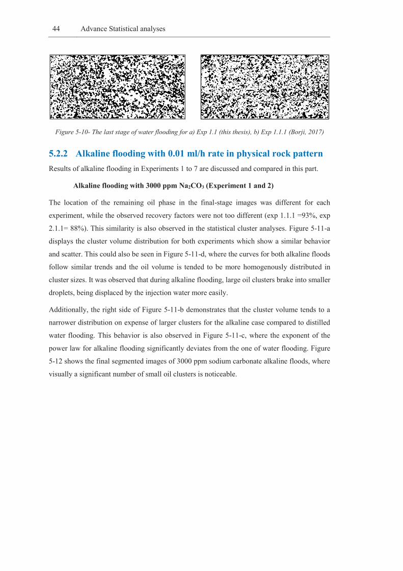
(Borji, 2017) a) Exp 1.1 (this thesis), b) Exp 1.1.1 for stage of water flooding lastThe -10-5Figure

5.2.2 Alkaline flooding with 0.01 ml/h rate in physical rock pattern Results of alkaline flooding in Experiments 1 to 7 are discussed and compared in this part.

Alkaline flooding with 3000 ppm Na2CO3 (Experiment 1 and 2)

The location of the remaining oil phase in the final-stage images was different for each

experiment, while the observed recovery factors were not too different (exp 1.1.1 =93%, exp

2.1.1= 88%). This similarity is also observed in the statistical cluster analyses. Figure 5-11-a

displays the cluster volume distribution for both experiments which show a similar behavior

and scatter. This could also be seen in Figure 5-11-d, where the curves for both alkaline floods

follow similar trends and the oil volume is tended to be more homogenously distributed in

cluster sizes. It was observed that during alkaline flooding, large oil clusters brake into smaller

droplets, being displaced by the injection water more easily.

Additionally, the right side of Figure 5-11-b demonstrates that the cluster volume tends to a

narrower distribution on expense of larger clusters for the alkaline case compared to distilled

water flooding. This behavior is also observed in Figure 5-11-c, where the exponent of the

power law for alkaline flooding significantly deviates from the one of water flooding. Figure

5-12 shows the final segmented images of 3000 ppm sodium carbonate alkaline floods, where

visually a significant number of small oil clusters is noticeable.


1 10 100 1000 10000 100000

1

10

100

1000

10000

Exp 1.1.1 Exp 2.1.1

Cou

nt


3000 ppm Sodium carbonate AF

1 10 100 1000 10000 100000

1

10

100

1000

10000

Exp 1.1 Exp 2.1 Exp 1.1.1 Exp 2.1.1

Cou

nt


3000 ppm Sodium carbonate AF and WF

(a)

(b)


Figure 5-11- Statistical analyses for 3000 ppm Na2CO3 a) cluster size distribution for AF, b) cluster

size distribution for WF and AF, c) Normalize distribution, d) Lorenz plot

Figure 5-12- Last stage of 3000 ppm flooding Na2CO3, a) Exp 1.1.1, b) Exp 2.1.1

(b)

(c)

(a)

(d)


Alkaline flooding with 7500 ppm Na2CO3 (Experiments 3 and 4)

Both of the following 7500 ppm Na2CO3 alkaline flooding experiments were repeatable in the

sense of recovery which was 80% for both, and also from the cluster statistical point of view,

even if the left image shows a large remaining cluster not observed in the right image (Figure

5-13). This is reflected in the images. Figure 5-14 discussing the statistical cluster properties.

With respect to the time dependent displacement, larger clusters break into smaller clusters,

which are mobile and finally recovered. However, even with similar cluster size distribution

(Figure 5-14-a), higher alkaline concentration generates larger clusters compared to 3000 ppm

Na2CO3 (comparing Figure 5-13 and Figure 5-13). The larger clusters and the resulting lower

recovery are due to microemulsion formation, which is pinning the clusters to the solid

boundaries. Overall, despite the discussed differences, the observed behavior is very similar to

that observed for the lower concentration of 3000 ppm Na2CO3.

Figure 5-13- Last stage of 7500 ppm Na2CO3 flooding a) Exp 3.1.1, b) Exp 4.1.1

1 10 100 1000 10000 100000

1

10

100

1000

10000

Exp 3.1.1 Exp 4.1.1

Cou

nt


7500 ppm Sodium carbonate AF (a)

(a) (b)


1 10 100 1000 10000 100000

1

10

100

1000

10000

Exp 3.1 Exp 4.1 Exp 3.1.1 Exp 4.1.1

Cou

nt


7500 ppm Sodium carbonate AF and WF (b)

(c)


Figure 5-14- Statistical analyses for 7500 ppm Na2CO3 a) cluster size distribution for AF, b) cluster

size distribution for WF and AF, c) Normalize distribution, d) Lorenz plot

Synthetic AF with 3000 and 7500 ppm Na2CO3 (Experiments 5 and 6)

Compared to water flooding with distilled water, synthetic water floods show a significant

higher recovery. However, an alkaline solution with synthetic water did not result in

considerable recovery (Figure 5-15). It should be mentioned that the IFT value for 3000 and

7500 ppm Na2CO3 solutions on basis of synthetic water are respectively 0.15 mN/m and 0.3

mN/m (Arnold, 2018), which are one order of magnitude higher than pure synthetic water.

Figure 5-15- Synthetic flooding a) Experiment 5.1, b) Experiment 5.1.1, c) Experiment 6.1 d)

Experiment 6.1.1

(a)

(c)

(b)

(d)

(d)


Even though the clusters break down as in the formerly discussed alkaline cases, cluster tends

to remain in the porous medium which is indicated in the cluster size distribution in Figure

5-16-b; the power law exponent fitted to the cumulative distributions for water and alkaline

flooding did not change, but shifts to smaller cluster sizes. Interestingly, the Lorenz curve

shows the same behavior before and after alkaline flooding, but are different for the two

synthetic water. Note that, no microemulsion was observed in synthetic floods.

1 10 100 1000 10000 100000 1000000

1

10

100

Exp 5.1 Exp 5.1.1 Exp 6.1 Exp 6.1.1

Cou

nt


(a)

(b)


Figure 5-16- Statistical analyses for synthetic WF and AF, a) cluster size distribution for WF and AF,


All the distilled alkaline flooding with 0.01 ml/h (Experiments 1-4 and 7)

In an additional experiment, 720 ppm NaOH was injected with the same injection rate. The

results are compared in the following to the results discussed before for 3000 and 7500 ppm

Na2CO3. Figure 5-17-a and Figure 5-17-b show the last stage of floods for 3000 ppm and 7500

ppm Na2CO3, respectively and is compared to the NaOH experiment in Figure 5-17-c.

Additionally, the IFT value for both concentration of Na2CO3 is the same and give as 0.065

mN/m (Arnold, 2018). Note that microemulsion generation was observed for 7500 ppm

Na2CO3 concentration in both, microfluidics and spinning drop (Arnold2018). Figure 5-18

shows that generated microemulsion is pinning the cluster on solid surfaces in micromodel.

Moreover, 3000 ppm Na2CO3 and 720 ppm NaOH show similar tertiary recovery factors, but

different displacement processes are observed. In Na2CO3 flooding, residual oil is recovered

from dead-end pores, while with NaOH, oil remains in dead-end pores.

(c)


Figure 5-17- Process images of the final stage, a) Exp 2.1.1 (3000 ppm Na2CO3), b) Exp 4.1.1 (7500

ppm Na2CO3), c) Exp 7.1.1 (720 ppm NaOH)

(a)

(b)

(c)


Figure 5-18- Pinned clusters due to microemulsion in 7500 ppm Na2CO3 in different pore volume

The microemulsion generation during 7500 ppm concentration was shown in Figure 5-19. After

15 pore volumes injection, the phase separation is observed.

Figure 5-19- Microemulsion generation in 7500 ppm Na2CO3 flooding in different pore volume

(PV= 9) (PV= 10.5)

(PV= 12) (PV= 15)

(PV= 9)

(PV= 15)


Comparing the generated droplet’s shape in micromodel with the spinning drop, the droplets in

3000 ppm Na2CO3 are separated and have regular distance from each other (Figure 5-20-a),

while the droplets are attached together in 7500 ppm concentration (Figure 5-20-b).

Figure 5-20- Images of droplets in micromodel and spinning drop of Na2CO3 a)3000 ppm, b) 7500

ppm

Comparing all the water flooding experiments with subsequent alkaline flooding at a single

flow rate, it is observed that the cluster sizes after alkaline floods are smaller compared to prior

water flooding (Figure 5-21-a). Moreover, Figure 5-21-b shows the water floods have a higher

probability of the larger cluster volume compare to the alkaline flooding. Besides, the fitted

power laws exponents in waterflooding have a similar trend. This similarity in a different way

is also observed in the alkaline flooding, except experiment 7.1.1, where too little clusters of

oil remained in the micromodel to make a reasonable statistic. In conclusion, this graph is

demonstrated a significant fingerprint for identifying and discriminating water and alkaline

flooding and their behavior. Additionally, a clear trend has been identified in the Lorenz plots,

where alkaline flooding experiments generated more homogeneous cluster volume distribution

than water floods (Figure 5-21-c).

(a)

(b)


1 10 100 1000 10000 100000

1

10

100

1000

10000

Exp 1.1 Exp 2.1 Exp 3.1 Exp 4.1 Exp 7.1 Exp 1.1.1 Exp 2.1.1 Exp 3.1.1 Exp 4.1.1 Exp 7.1.1

Cou

nt


All flooding with 0.01 ml/hr

(b)

(a)


Figure 5-21- Statistical analyses for all flooding with 0.01 ml/h, a) cluster size distribution for WF and

AF, b) Normalize distribution, c) Lorenz plot

5.2.3 Different injection rate in physical rock pattern (Experiments 7

and 9) The comparison of water flooding using different injection rates results in a minor change in

recovery factor which is about ~43%. However, with lower injection rate, the bypassing of oil

or channeling is more likely to occur forming preferred pathways. In Figure 5-22-a, such

pathways are visible in top and bottom of micromodel.

Nevertheless, the difference is more significant in alkaline flooding, where the recovery is

lower for the lower injection rate. This performance can be described by the capillary number,

where all the parameters are constant but the flow rate and hence the viscous force, where a

higher flow rate means a higher capillary number. Therefore, the small droplets are remaining

in the micromodel. In Figure 5-22-b, the small droplets are observed which are not recovered

from the system in comparison to Figure 5-17-c, where most of the cluster are displaced from

the porous domain.

(c)


Figure 5-22- Last stage of flooding a) water, b) 720 ppm NaOH flooding

The cluster-volume size distribution illustrated that most of the small droplets are recovered

from micromodel in the alkaline floods with higher injection rate (Experiment 7.1.1). In the

case of lower injection rate (Experiment 9.1.1), the large clusters break into smaller clusters

that mainly remain in the system (Figure 5-23-a). In Figure 5-23-b and Figure 5-23-c, similar

trends for water and alkaline flooding were found, indicating that cluster size distribution is

largely independent of flow rate.


1 10 100 1000 10000 100000 1000000

1

10

100

Exp 7.1 Exp 9.1 Exp 7.1.1 Exp 9.1.1

Coun

t


720 ppm NaOH with different injection rate

(b)

(a)


Figure 5-23- Statistical analyses for NaOH with different injection rate, a) cluster size distribution for

WF and AF, b) Normalize distribution, c) Lorenz plot

5.2.4 Alkaline flooding with 0.001 ml/h rate in physical rock pattern Results of alkaline flooding where microemulsion formation was observed are discussed and

compared in the following.

720 ppm NaOH and 6000 ppm Na2CO3 (Experiments 9 and 12)

Comparing cluster sizes of experiment 9 (720 ppm NaOH) with experiment 12 (6000 ppm

Na2CO3), were more abundant compared to experiment 12 (6000 ppm Na2CO3). This behavior

is observed by comparing Figure 5-22-b and Figure 5-24. In both solutions, the microemulsion

was formed. However, the microemulsion in 6000 ppm Na2CO3 was more visible during the

experiments and reduced the oil production by pinning the cluster on the solid boundaries.

Figure 5-25 shows the generated microemulsion in experiment 12 (6000 ppm Na2CO3).

(c)


Figure 5-24- Last stage of experiment 12.1.1 (6000 ppm Na2CO3)

Figure 5-25- Microemulsion in experiment 12.1.1 (6000 ppm Na2CO3)

Comparing the water flooding experiments with subsequent alkaline flooding in lower injection

rate, the similar trend as high injection rate is observed, where the cluster sizes after alkaline

floods are smaller compared to prior water flooding (Figure 5-26-b). However, a different

behavior was observed in the Lorenz plot for 6000 ppm Na2CO3 compared to 720 ppm NaOH

(Figure 5-26-c), which is probably due to the microemulsion generation.


1 10 100 1000 10000 100000 1000000

1

10

100

Exp 9.1 Exp 9.1.1 Exp 12.1 Exp 12.1.1

Cou

nt


720 ppm NaOH and 6000 ppm Na2CO3

(a)

(b)


Figure 5-26- Statistical analyses for 6000 ppm Na2CO3 and 720 ppm NaOH, a) cluster size

distribution for WF and AF, b) Normalize distribution, c) Lorenz plot

Experiments with microemulsion generation

Cluster size distribution is investigated by analyzing experiment 12.1.1 (6000 ppm Na2CO3)

and 720 ppm sodium hydroxide in (Borji, 2017), where the enormous volume of microemulsion

was observed. The interesting point is that in both experiments, the cluster size distribution is

demonstrating the similar behavior (Figure 5-27).

1 10 100 1000 10000 100000 1000000

1

10

100

Exp 12.1.1 Borji 720 ppm Naoh

Cou

nt


Experiments with Microemulsion (a)

(c)


Figure 5-27- Statistical analyses for microemulsion generation, a) cluster size distribution for AF, b)

Normalize distribution, c) Lorenz plot

5.2.5 Flooding in the uniform pattern Waterflooding

The range of oil recovery for waterflooding in this pattern was between 40% to 50%. This

variation might be due to channeling in the micromodel induced by displacement instabilities.

Two channels in the upper and bottom part of the flooding domain were generated during water

(b)

(c)


flooding. Note that the main contrast between these floods was the displacement of oil through

these channels. In more details, the secondary drainage occurs in this process, which is shown

in Figure 5-28. The red square in Figure 5-28-a illustrates the spot, where the oil was swept

after exposing to water after 0.4 pore volume of water injection. However, Figure 5-28-b shows

that oil reinvaded water-flooded zones (secondary oil drainage) after 0.45 pore volume of water

injection. In experiment 10.1 (Figure 5-29-a), besides the channeling in the top and bottom of

the micromodel, oil in the middle of the micromodel was swept. In experiment 11.1 the

channels are the main flow path, which is shown in Figure 5-29-b. In contrast, the channels

were mostly blocked by oil after the secondary drainage in experiment 13.1, which is illustrated

in Figure 5-29-c. Capillary fingering is considered as the displacement process for all of these

floodings, where the logarithm of the capillary and mobility number is ~ -5 and 3, respectively.

Based on Figure 2-5, they are located in capillary fingering domain of the diagram.

Figure 5-28- Secondary drainage in the uniform pattern

PV= 0.4

PV= 0.45

(a)

(b)


Figure 5-29- Binary image at the final stage of a) Experiment 10.1, b) Experiment 11.1, c) Experiment

13.1

Alkaline Flooding

In Figure 5-30-a, the alkaline flooding of experiment 10.1.1 (720 ppm NaOH) is shown. The

results showed that oil production is mostly dependent on the pathways of the waterflood before

the alkaline flooding. This is mainly due to the aqueous phase flowing in the initially created

channels and the oil in between was mainly untouched. In Figure 5-30-b, the alkaline solution

(950 ppm Na2CO3) swept the oil from inlet channels and changed oil saturation in the

micromodel. However, the highest sweep efficiency was observed in experiment 13.1.1 (6000

(b)

(c)

(a)


ppm Na2CO3), where new channels were created during alkaline flooding (Figure 5-30-c).

Hence, the quantitative comparison between different alkali solution in this pattern made not

much sense. However, the capillary fingering is considered as a displacement process in these

experiments same as waterflooding. The statistical analyses did not show any specific trend,

which may have to do with the fact that the displacement is dominated by sweep effects and

early breakthrough (Figure 5-31).

Figure 5-30- Binary image at the final stage of a) Experiment 10.1.1(720 ppm NaOH), b) Experiment

11.1.1(950 ppm Na2CO3), c) Experiment 13.1.1(6000 ppm Na2CO3)

(c)

(a)

(b)


10 100 1000 10000 100000 1000000

1

10

100

1000 Exp 10.1 Exp 10.1.1 Exp 11.1 Exp 11.1.1 Exp 13.1 Exp 13.1.1

Cou

nt


Experiments in Uniform pattern

(b)

(a)


Figure 5-31- Statistical analyses for the uniform pattern, a) cluster size distribution for WF and AF,


5.2.6 Comparison between two patterns Ganglion dynamic and traffic flows droplets were observed in the uniform pattern experiments,

while capillary forces disconnected the phases and formed small oil droplet (Figure 5-32-a). In

addition, the capillary forces are lower in the physical rock pattern and the snap off was mainly

observed due to the change of wetting conditions leading to a dispersion of the oil phase in

small droplets (Figure 5-32-b).

Figure 5-32- Flow pattern for a) Uniform, b) Physical rock

(c)

(a)

(b)

Capillary Desaturation curve 69

5.3 Capillary Desaturation curve The capillary desaturation curve is plotted for the experiments by using the IFT value in Figure

5-33. As expected, water floods with lower injection rate (0.001 ml/h) have the least capillary

number through all the experiments. In contrast, synthetic water flooding has the maximum

capillary number. This graph illustrated that the critical capillary number is around 10-4, where

the residual oil saturation is reduced. Furthermore, the waterfloods mainly fall on the plateau

region, where changing the injection rate (velocity) has a minor impact on the reduction of the

residual oil saturation in the experiments.

Figure 5-33- Capillary desaturation curve for the experiments

Chapter 6

Conclusion

6.1 Summary In the frame of this thesis, alkaline flooding was investigated by using microfluidics. Several

experiments have been performed under different conditions to study the effects of:

Micromodel pattern types (physical rock and uniform)

Alkaline type and concentration (Na2CO3 and NaOH)

Water composition (pure water and synthetic water)

Injection rate (0.01 ml/h and 0.001 ml/h).

The image processing shows that the recovery results have inconsistencies in the experiments

due to the flooding domain which was not representing an elementary volume for two phase

flow, which is a common problem in the area of pore-scale physics. Therefore, discrete

frequency distributions, cumulative distributions and Lorenz plots, have been used to

understand the performance of EOR processes by statistical means. Based on the obtained

results statistical fingerprints have been found to describe the performance and mechanisms for

water and alkaline flooding.

Upon visual observation, the synthetic water displaced a significant amount of oil compared to

the distilled-water flood. In addition, the 3000 ppm Na2CO3 used in tertiary recovery,

demonstrated an optimum displacement with respect to other concentration. This could be due

to the reduced microemulsion generations. Among the two injection rates, the waterflooding

showed the minor effect on oil recovery. However, in the case of 720 ppm NaOH flooding, the

lower injection rate resulted in lower recovery due to lower viscous forces applied.

72 Future Work

Additional experiments on the regular pore network showed that the displacement is dominated

by capillary fingering. The displacement patterns stay in strong contrast to the displacement

characteristics in the physical rock pattern.

6.2 Future Work Further work for better understanding EOR chemical processes are recommended:

Generation of capillary desaturation curve using a wide range of chemicals and

injection rates

Performing polymer-alkaline flooding in the uniform and non-uniform micromodel

patterns to study the effect of capillary to viscous forces

Studying the microemulsion generation and its impact on oil production

Designing a new micromodel facilitating higher capillary contrast

Investigating different displacement processes based on Lenormand plot’s.

Chapter 7

References A. Chatenever, J. Calhoun, 1952. Visual examinations of fluid behavior in porous media.

PETROLEUM TRANSACTIONS, Volume 195, pp. 149-156.

A. Georgiadis, S. Berg, A. Makurat, G. Maitland, H. Ott, 2013. Pore-scale micro-computed-

tomography imaging: Nonwetting-phase cluster-size. PHYSICAL REVIEW, 88(3).

A. Lucian, R. Hilfer, 1999. Trapping and mobilization of residual fluid during capillary

desaturation in porous media. PHYSICAL REVIEW E, 59(6), p. 6819–6823.

Aaron Clauset, Cosma Rohilla Shalizi, M. E. J. Newman, 2009. Power-Law Distributions in.

Society for Industrial and Applied Mathematics, Volume 51, pp. 661-703.

Anon., n.d. Dmi8 Leica. [Online]

Available at: https://www.leica-microsystems.com/products/light-microscopes/inverted-

microscopes/details/product/leica-dmi8/

Arnold, P., 2018. Experimental investigation of interfacial tension for alkaline flooding, s.l.:

Montan University Leoben.

Borji, M., 2017. Alkali-based Displacement Processes in Microfluidic Experiments:

Application to the Matzen Oil Field, s.l.: Montan University Leoben.

C. E. Cooke Jr., R. E. Williams, P. A. Kolodzie, 1974. Oil Recovery by Alkaline Waterfiooding.

PETROLEUM TECHNOLOGY, pp. 1366-1374.

C. E. Cooke, J. R. E. W. P. A. K., 1974. Oil Recovery by Alkaline Waterfiooding. SPE.

C. Mattax, J.R. Kyte, 1962. Imbibition Oil Recovery from Fractured, Water-Drive Reservoir.

SPE, 2(02), pp. 177-184.

74 Future Work

Cheng JT, Giordano N, 2002. Fluid flow through nanometer-scale channels. Physical Review,

p. 5.

Christophe Cottin, Hugues Bodiguel, Annie Colin, 2010. Drainage in two-dimensional porous

media: From capillary fingering to viscous flow. PHYSICAL REVIEW.

Dullien, F. A., 1979. Porous media fluid transport and pore structure. s.l.:ACADEMIC

PRESS.

E.F. deZabala, J. V. E. R. C. R., 1982. A Chemical Theory for Linear Alkaline Flooding. SPE.

Ehrlich R., Hasiba H.H., Raimondi P., 1974. Alkaline waterflooding for wettability alternation.

Petroleum Technology, pp. 1335-1352.

Hu Guo, Ma Dou, Wang Hanqing, Fuyong Wang, Gu Yuanyuan, Zhaoyan Yu, Wang

Yansheng, Yiqiang Li, 2017. Proper Use of Capillary Number in Chemical Flooding. Hindawi

Journal of Chemistry, Volume 2017, p. 11.

ImageJ, 2017. 3D_Objects_Counter. [Online]

Available at: https://imagej.net/3D_Objects_Counter

[Accessed 9 August 2018].

International Energy Agency, 2013. IEA, s.l.: International Energy Agency.

J. C. Melrose, C. F. Brandner, 1974. Role of Capillary Forces in Determining Microscopic

Displacement Efficiency for Oil Recovery by Waterflooding. The Journal of Canadian

Petroleum, pp. 54-62.

Jennings, H. Y., Jr., Johnson, C. E., Jr., and McAuliffe, C. D, 1974. Caustic Waterflooding

Process for Heavy Oils. Petroleum Technology, pp. 1344-1352.

Johnson, C. E., 1976. Status of Caustic and Emulsion Methods. PETROLEUM

TECHNOLOGY, pp. 85-92.

Lake, L. W., 1989. Enhanced oil recovery. s.l.:Prentice-Hall Inc., Englewood Cliffs.

Larry W. Lake, R. J. B. R. a. G. P., 2014. Fundamentals of Enhanced Oil Recovery. s.l.:Society

of Petroleum Engineers.

Micronit, 2018. Micronit Chipholder. [Online]

Available at: https://store.micronit.com/chipholders/fluidic-connect-4515-chipholder

Micronit, 2018. Micronit EOR micromodel. [Online]

Available at: https://store.micronit.com/microfluidic-chips/enhanced-oil-recovery-chips/3-

pack-eor-chips-physical-rock-network-443

Future Work 75

Mohsen Yeganeh, Jessica Hegner, Eric Lewandowski, Aruna Mohan, Larry W. Lake, Dan

Cherney, Arben Jusufi, Aditya Jaishankar , 2016. Capillary Desaturation Curve Fundamentals.

SPE , p. 14.

N. K. Karadimitriou and S. M. Hassanizadeh, 2012. A Review of Micromodels and Their Use

in Two-Phase Flow Studies. Vadose Zone, Volume 11.

Nutting, P. G., 1925. Chemical Problems in the Water Driving of Petroleum from Oil Sands.

Industrial and Engineering Chemistry.

O.R. Wagner, R.O. Leach, 1959. Improving Oil Displacement Efficiency by Wettability

Adjustment. Transactions of the AIME, 216(1), pp. 65-72.

Ott, H., 2018. Microfluidics for EOR Screening Application to Alkaline Flooding. Copenhagen,

EAGE.

Prosense, 2018. NE 300 Syringe pump. [Online]

Available at: http://www.prosense.net/prosense/product-database/ne300-single-syringe-pump-

just-infusion/2242

R. Lenormand, 1990. Liquids in porous media. Journal of Physics: Condensed Matter, Volume

2.

Riyaz Kharrat, A. R., 2017. Practical Improved Hydrocarbon Recovery: An Industrial Guide

Book for EOR and IOR. s.l.:LAP LAMBERT Academic Publishing.

Roland Lenormand, Cesar Zarcone, 1985. Invasion Percolation in an Etched Network:

Measurement of a Fractal Dimension. Physical Review, pp. 2226-2230.

Ryan T. Armstrong, Apostolos Georgiadis, Holger Ott, Denis Klemin, Steffen Berg, 2014.

Critical capillary number: Desaturation studied with fast X-ray. GEOPHYSICAL RESEARCH

LETTERS, Volume 41, pp. 50-60.

S. Kokal, A. A.-K., 2010. Enhanced oil recovery: challenges & opportunities, s.l.: World

Petroleum Council.

Shao-Yiu Hsu, Zhong-Yao Zhang, Chia-Wen Tsao, 2017. Thermoplastic Micromodel

Investigation of Two-Phase Flows in a Fractured Porous Medium. Micromachines.

Sheng, J. J., 2011. Modern Chemical Enhanced Oil Recovery. s.l.:Gulf Professional Publishing.

Sheng, J. J., 2013. Enhanced Oil Recovery Field Case Studies. s.l.:Gulf Professional

Publishing.

Sheng, J. J., 2015. Status of Alkaline Flooding Technology. Petroleum Engineering &

Technology, Volume 5, pp. 44-50.

76 Future Work

Squires, F., 1917. Recovery of oil from oil-sands. United States of America, Patent No.

1238355A.

Subkow, P., 1942. Process for the removal of bitumen from bituminous deposits. United States

of America, Patent No. 2288857.

Y. Alzahid, P. MOstaghimi, M. Ebrahimi Warkiani, R T. Armstrong, 2017. Alkaline Surfactant

Polymer Flooding: What happens at the pore scale. SPE, p. 17.

Yi‐Feng Chen, Shu Fang, Dong‐Sheng Wu, Ran Hu, 2017. Visualizing and quantifying the

crossover from capillary fingering to viscous fingering in a rough fracture. Water Resources

Research, 53(9), pp. 7756-7772.

alkali-based displacement processes in microfluidic ...in this thesis, alkaline flooding was...

Documents