(almost) model-free recovery - brown university · (almost) model-free recovery paul schneideryand...

(Almost) Model-Free Recovery∗

Paul Schneider†and Fabio Trojani‡

August 10, 2015

Abstract

Based on mild economic assumptions, we recover the time series of

conditional physical moments of market index returns from a model-

free projection of the pricing kernel on the return space. These mo-

ments identify the minimum variance pricing kernel projection and

are supported by a corresponding set of physical distributions. The

recovered moments predict S&P 500 returns, especially for longer hori-

zons, give rise to refined conditional versions of Hansen-Jagannathan

bounds, and can be traded using delta-hedged option portfolios. They

also imply conditional pricing kernel projections that are often far from

being uniformly monotonic and convex.

1 Introduction

A seminal finding in Breeden and Litzenberger (1978) shows that in an

arbitrage-free market the density of the conditional forward-neutral distri-

bution (QT ) of an asset return coincides with the second derivative of the

∗We are thankful for helpful discussions with Gianluca Cassese, Damir Filipovic, PatrickGagliardini, Peter Gruber, Olivier Scaillet, Christian Wagner and seminar participants ofthe USI brownbag workshop. Financial support from the Swiss Finance Institute (Project”Term structures and cross-sections of asset risk premia”), and the SNF (Project “TradingAsset Pricing Models”) is gratefully acknowledged.†Boston University, University of Lugano, and Swiss Finance Institute. Email:.

[email protected]‡University of Geneva, University of Lugano, and Swiss Finance Institute. Email:.

[email protected]

1

mailto:[email protected]

mailto:[email protected]

price function of European call options with respect to the option’s strike.

There is no such general and model-free result for the conditional distribution

of asset returns under the physical probability measure (P).

To learn more about physical distributions, researchers often have made

use of parametric modelling approaches (e.g., Jones, 2003; Eraker, 2004).

In these models, probabilities P and QT are usually linked by a paramet-

ric (forward) stochastic discount factor dQT/dP, which can be estimated

from historical return information and allows to uniquely recover P probabil-

ities from QT probabilities using this additional information. More recently,

some authors have derived recovery theorems based on a different set of non-

parametric assumptions. In a complete market setting with Markovian and

stationary state dynamics on a (bounded) finite state space, Ross (2015)

uniquely recovers a path-independent stochastic discount factor dQT/dP us-

ing Perron Frobenius theory. Borovicka et al. (2014) discuss in more detail

the implications of path-independence and emphasize that in general only a

misspecified probability measure can be recovered, different from the phys-

ical probability, which incorporates long-run risk adjustments. Hence, the

physical probability remains unidentified without introducing additional re-

strictions or using additional data.

We propose to identify the main characteristics of the physical probability

P with a conceptually different approach from the one adopted in existing

recovery theorems. Without making stringent assumptions about the under-

lying economy or price processes, we start from a set of plausible economic

assumptions on the sign of the risk premia for trading particular nonlinear

risks in option markets. While theoretically the forward equity premium,

the first conditional P moment of forward market returns, needs to be posi-

tive in equilibrium, additional natural assumptions can be motivated for the

risk premia on higher moments. For instance, it is widely recognized in the

theoretical and empirical literature that the price of market variance risk,

and more generally even market divergence risk, is negative; see Carr and

Wu (2009), Martin (2013) and Schneider and Trojani (2014), among others.

Similarly, the risk premium for exposure to odd market divergence risk, such

as skewness risk, is naturally positive, because it is generated by risks that

2

are monotonic transformations of market returns; see Kozhan et al. (2013)

and Schneider and Trojani (2014), among others.

A sign restriction on an asset risk premium is a constraint on the co-

variance between the pricing kernel and the return of that particular asset.

Given a set of observed prices of suitable option portfolios and a model-free

no-arbitrage condition, we show that this restriction implies useful model-

free constraints on the physical conditional moments of market returns. In

this way, we obtain a family of model-free upper and lower bounds on differ-

ent conditional moments of market returns, which extend the lower bound in

Martin (2015) for the market equity premium. We show that these bounds

are highly time-varying, reflecting a rich conditional distribution of market

returns, and that they imply relatively tight intervals for the unknown phys-

ical moments of market returns.

Our model-free bounds on the physical conditional moments effectively

constrain the set of physical probabilities that in abitrage-free markets can

support (i) our economic risk premium constraints and (ii) the observed

prices of suitable option portfolios. We characterize the admissible moments

supported by a probability measure satisfying conditions (i), (ii), using known

results on the solution of (truncated) moment problems.1 In this way, we

obtain a parsimomious description of the family of physical moments for

which a model-free recovery result can be motivated.

We obtain recovery based on a model-free L2−projection of the pric-

ing kernel on market returns. This projection is parameterized by forward-

neutral and physical moments alone. Therefore, any parameterization con-

sistent with our physical moment constraints and with the prices of suitable

option portfolios defines an admissible physical measure P in our incomplete

market setting.2 We focus on model-free recovery of the minimal variance

physical measure, which implies the tightest upper bound on the Sharpe ratio

1Moment problems (truncated moment problems) deal with the question of whether fora given countable (finite) sequence of numbers there exists a probability measure havingthese numbers as its moments.

2 As the number of constrained physical and forward-neutral moments goes to infinity,our L2projection parameterization converges to the physical expectation of the pricingkernel conditional on forward market returns.

3

of any portfolio of asset returns that are exactly priced by the projection.

Using our economically motivated model-free recovery, we avoid a number

of strong technical assumptions on the underlying economy, which might be

difficult to motivate or to test in practice. For instance, we do not need

strong assumptions on the economy state space or the underlying stochastic

processes, such as the Markovianity or the stationarity of asset returns, nor

do we need to assume path-independent pricing kernels. We can assume a

weak model-free definition of arbitrage opportunities to invoke model-free

versions of the fundamental theorem of asset pricing (Acciaio et al., 2013)

and ensure existence of a forward-neutral measure in our setting. For the

existence of our L2 pricing kernel projection, we need the existence of all

polynomial moments of market returns, which is ensured, for example, if the

state space of market returns is conditionally bounded. Boundedness of the

state space is assumed in virtually all recovery theorems in the literature.

Moreover, from our treatment based on truncated moment problems, the

recovered physical probability in our incomplete market setting can indeed

be ensured to have bounded support. Clearly, the cost of the generality of

our approach in terms of weak technical conditions arises from the economic

assumptions about the risk premia of particular asset returns, which might

however by easier to motivate and test in some cases.

We find that the conditional moments implied by our recovered pricing

kernel projections are highly time-varying and informative about future mar-

ket realizations, especially for longer horizons. Our technology also naturally

recovers second conditional moments of nonlinear minimum variance pricing

kernel projections, which extend the linear projection approach in Hansen

and Jagannathan (1997). We document large Sharpe ratios from option

strategies trading the different moments of the pricing kernel projection. The

conditional projections themselves suggest frequent departures from mono-

tonicity and convexity. Precisely, higher-order projections frequently exhibit

a u-shape at short maturities of 1 month, in line with Beare and Schmidt

(2014) and Bakshi et al. (2010), implying an average unconditional projec-

tion that is concave (convex) in regions of low (large) returns. For longer

maturities, the average unconditional projection is concave everywhere.

4

Our paper borrows from several strands in the literature. Chapman

(1997) investigates consumption-based asset pricing models unconditionally

using technology similar to ours. Aıt-Sahalia and Lo (1998) estimate the

state price density (the product of the pricing kernel projection and the phys-

ical probability measure) using kernel regression. Their approach requires a

choice of regressors and uses information from the entire sample history of

option prices. Song and Xiu (2014) exploit also the information contained in

VIX options. Jackwerth (2000) investigates the marginal rate of substitution

in a complete market. Aıt-Sahalia and Duarte (2003) and Birke and Pilz

(2009) develop a polynomial kernel projection which maintains convexity of

option prices in strike. Aıt-Sahalia and Lo (2000) learn about the marginal

rate of substitution from time series data and option prices.

There is also a related literature on inequalities for moments of asset

prices and the pricing kernel. Alvarez and Jermann (2005) develop bounds

on the pricing kernel along with a decomposition under the maintained as-

sumption that it is a stationary stochastic process. Hansen and Scheinkman

(2009) obtain a similar decomposition under an additional Markov assump-

tion. Martin (2015) derives a lower bound of the equity premium from a

negative covariance condition, a joint restriction on the pricing kernel and

the market return. Julliard and Ghosh (2012) develop an empirical like-

lihood estimator of a consumption-based pricing kernel. This approach is

extended in Gosh et al. (2013) along with entropy bounds for the pricing

kernel. Within the same methodological framework, Almeida and Garcia

(2015) compute a family of discrepancy bounds for pricing kernels. Carr and

Yu (2012) trade in the discrete state assumption in Ross (2015) mentioned

above for the family of bounded diffusion processes. Borovicka et al. (2014)

show that Ross (2015) recovery reveals the physical conditional density only

under additional technical conditions.

This paper first develops asset pricing bounds on moments of the S&P 500

in Section 2. Subsequently it puts these bounds to use to parameterize pricing

kernel projections in Section 3. An empirical study uses these projections

in an empirical study in Section 4. Section 5 concludes and the Appendix

contains additional computations B, figures and tables in Section C.

5

2 Bounds on Conditional Polynomial Mo-

ments of the Market

In this Section we develop upper and lower bounds on polynomial moments

under the true, unobserved physical P measure of gross forward returns

R :=FT,T

Ft,T∈ D ⊂ R+, where Ft,T is the forward price at time t of the

spot S&P 500 for delivery at time T ≥ t. We refer to R as the gross market

return. Under no-arbitrage the true and unobserved forward pricing kernel

and its expectation conditional on a time-T−measurable random variable R

are denoted by

MP =dQT

dP, and MP(R) := EP [MP | R] , (1)

where QT denotes the forward martingale measure associated with the zero

coupon bond numeraire. We introduce this notation anticipating our focus on

P, and that a representative QT of forward-neutral measures can be inferred

from option prices. This paper is based on model-independent arguments

in the sense that we do not assume an underlying stochastic process for R.

In our context it is therefore instructive to take D to be a compact subset

of R+, as this ensures, together with sufficiently many options written on

R, a model-free fundamental theorem of asset pricing (Acciaio et al., 2013,

Remark 2.4).

We next introduce notation that will help us in the context of financial

markets equipped with European options. The time-dependent operator Jttakes a function f , twice differentiable almost everywhere, and approximates

it in a piece-wise linear fashion inside a certain corridor, and linearizes the

6

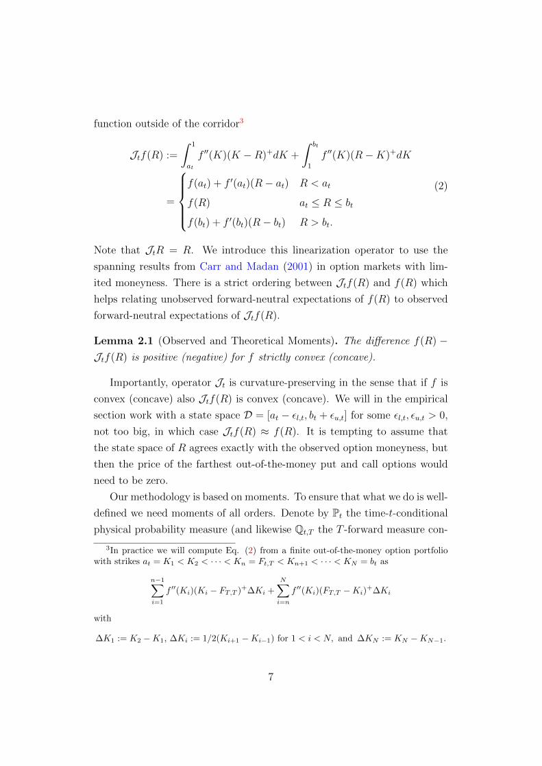
function outside of the corridor3

Jtf(R) :=

∫ 1

at

f ′′(K)(K −R)+dK +

∫ bt

1

f ′′(K)(R−K)+dK

=

f(at) + f ′(at)(R− at) R < at

f(R) at ≤ R ≤ bt

f(bt) + f ′(bt)(R− bt) R > bt.

(2)

Note that JtR = R. We introduce this linearization operator to use the

spanning results from Carr and Madan (2001) in option markets with lim-

ited moneyness. There is a strict ordering between Jtf(R) and f(R) which

helps relating unobserved forward-neutral expectations of f(R) to observed

forward-neutral expectations of Jtf(R).

Lemma 2.1 (Observed and Theoretical Moments). The difference f(R) −Jtf(R) is positive (negative) for f strictly convex (concave).

Importantly, operator Jt is curvature-preserving in the sense that if f is

convex (concave) also Jtf(R) is convex (concave). We will in the empirical

section work with a state space D = [at − εl,t, bt + εu,t] for some εl,t, εu,t > 0,

not too big, in which case Jtf(R) ≈ f(R). It is tempting to assume that

the state space of R agrees exactly with the observed option moneyness, but

then the price of the farthest out-of-the-money put and call options would

need to be zero.

Our methodology is based on moments. To ensure that what we do is well-

defined we need moments of all orders. Denote by Pt the time-t-conditional

physical probability measure (and likewise Qt,T the T -forward measure con-

3In practice we will compute Eq. (2) from a finite out-of-the-money option portfoliowith strikes at = K1 < K2 < · · · < Kn = Ft,T < Kn+1 < · · · < KN = bt as

n−1∑i=1

f ′′(Ki)(Ki − FT,T )+∆Ki +

N∑i=n

f ′′(Ki)(FT,T −Ki)+∆Ki

with

∆K1 := K2 −K1, ∆Ki := 1/2(Ki+1 −Ki−1) for 1 < i < N, and ∆KN := KN −KN−1.

7

ditional on time t information) generating the conditional expectations EPt [·],

respectively EQTt [·].

Lemma 2.2 (Existence of Moments). The moment-generating functions

EPt

[eu·R

], and EQT

t

[eu·R

](3)

exist for u ∈ R+.

The compactness of the state space D guarantees integrability even for

fat-tailed distributions.4 A computation shows that Lemma 2.2 also guaran-

tees existence of moments of discrete returns Re := R− 1, and corridor mo-

ments JtRn. Denote the conditional monomial moments by µPt,n := EP

t [Rn]

and µQTt,n := EQT

t [Rn], respectively. The next assumption is on expected

profits of trading strategies with exposure to nonlinear functions of R.

Assumption 1 (Negative Divergence Premium (NDP)). With power diver-

gence function

Dp(R) :=Rp − pR + p− 1

p2 − p,

D1(R) := R log(R)−R + 1, and D0(R) := R− log(R)− 1,

(4)

we define the negative n-power divergence premium NDP(p,n) assumption

of orders p and n as the inequality

− CovPt [M,JtDp(Rn)] = −CovPt [M(R),JtDp(R

n)] ≤ 0. (5)

Power divergence swaps introduced by Schneider and Trojani (2015) pay-

ing the difference between realized and implied divergence5 can be replicated

4Standard models on unbounded state spaces such as Black-Scholes or Heston (1993)do not satisfy the requirement of a compact state space necessary for Lemma 2.2, but theyare relatively easy to compactify. We use them in Figure 4 to illustrate model likelihoodratios.

5In their construction realized divergence depends on the path of the forward pricefrom time t to time T , but all payoffs arise at time T , such that there is no differencebetween pricing with MP, or MP(R).

8

from option data. Together with the identity

Dp(Rn) =

n

p− 1[(np− 1)Dpn(R)− (n− 1)Dn(R)] , with

D1(Rn) := lim

p→1

n

p− 1[(np− 1)Dpn(R)− (n− 1)Dn(R)]

= nRn log(R)−Rn + 1,

(6)

Assumption 1 is therefore empirically testable unconditionally, since both

Dpn(R) and Dn(R) are tradeable quantities. From Assumption 1 and

Jensen’s inequality we directly get

Proposition 2.3 (Upper Bounds on Conditional P Moments). NDP (p, n)

holds if and only if

S(JtDp(Rn)) := EQT

t [JtDp(Rn)] ≥ EP

t [JtDp(Rn)] ≥ JtDp(EP

t [Rn]). (7)

From Proposition 2.3 above we define implicitly the upper bound on the

n-th moment of R, µPuppert,n , as the solution to

S(JtDp(Rn)) = JtDp(µ

Puppert,n ). (8)

The NDP from Assumption 1 establishes relations between QT and P mo-

ments of different orders by varying p and n and therefore entails economic

information beyond Proposition 2.3. The next assumption is harder to test

empirically.

Assumption 2 (Negative Covariance Condition (NCC)). For p, q ∈ R we

define the negative covariance condition NCC(p, q) as the inequality

CovPt [MRq, Rp] = CovPt [M(R)Rq, Rp]

= EQTt

[Rp+q

]− EQT

t [Rq]EPt [Rp] ≤ 0.

(9)

To adapt Assumption 2 to finite option markets we employ Lemma 2.1

9

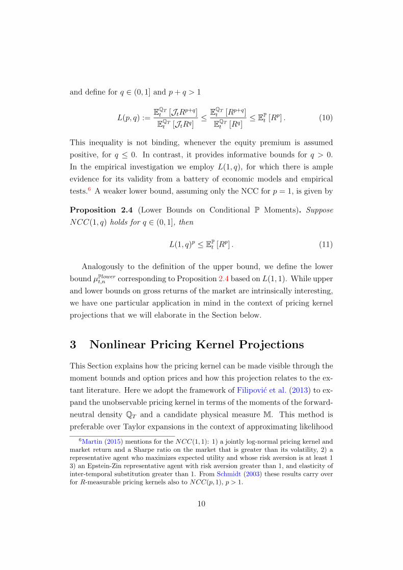
and define for q ∈ (0, 1] and p+ q > 1

L(p, q) :=EQTt [JtRp+q]

EQTt [JtRq]

≤ EQTt [Rp+q]

EQTt [Rq]

≤ EPt [Rp] . (10)

This inequality is not binding, whenever the equity premium is assumed

positive, for q ≤ 0. In contrast, it provides informative bounds for q > 0.

In the empirical investigation we employ L(1, q), for which there is ample

evidence for its validity from a battery of economic models and empirical

tests.6 A weaker lower bound, assuming only the NCC for p = 1, is given by

Proposition 2.4 (Lower Bounds on Conditional P Moments). Suppose

NCC(1, q) holds for q ∈ (0, 1], then

L(1, q)p ≤ EPt [Rp] . (11)

Analogously to the definition of the upper bound, we define the lower

bound µPlowert,n corresponding to Proposition 2.4 based on L(1, 1). While upper

and lower bounds on gross returns of the market are intrinsically interesting,

we have one particular application in mind in the context of pricing kernel

projections that we will elaborate in the Section below.

3 Nonlinear Pricing Kernel Projections

This Section explains how the pricing kernel can be made visible through the

moment bounds and option prices and how this projection relates to the ex-

tant literature. Here we adopt the framework of Filipovic et al. (2013) to ex-

pand the unobservable pricing kernel in terms of the moments of the forward-

neutral density QT and a candidate physical measure M. This method is

preferable over Taylor expansions in the context of approximating likelihood

6Martin (2015) mentions for the NCC(1, 1): 1) a jointly log-normal pricing kernel andmarket return and a Sharpe ratio on the market that is greater than its volatility, 2) arepresentative agent who maximizes expected utility and whose risk aversion is at least 13) an Epstein-Zin representative agent with risk aversion greater than 1, and elasticity ofinter-temporal substitution greater than 1. From Schmidt (2003) these results carry overfor R-measurable pricing kernels also to NCC(p, 1), p > 1.

10

ratios for a number of reasons. Firstly, economic restrictions such as pricing

constraints are automatically built in. Secondly, the projection is by con-

struction a M martingale. Thirdly, it accommodates easily economies with

pricing kernels that are not measurable with respect to the asset the pricing

kernel is projected on. We work here with polynomial projections, although

other bases are thinkable and maybe even preferable for some applications.

For the purpose of using the projection theorem we introduce the notion of

square integrability.

Definition 3.1. Define the weighted Hilbert space L2M as the set of (equiva-

lence classes of) measurable real-valued functions f on R with finite L2M-norm

‖f‖2L2M =

∫Rf(ξ)2 dM(ξ) <∞. (12)

Accordingly, the scalar product on L2M is denoted by

〈f, h〉L2M =

∫Rf(ξ)h(ξ) dM(ξ). (13)

Assumption 3 (Finite Pricing Kernel Variance). For given probability mea-

sure MMM ∈ L2

M. (14)

Assumption 3 states that the variance of the pricing kernel is finite,

a common assumption necessary for example for the existence of Hansen-

Jagannathan and good deal bounds (Cochrane and Saa-Requejo, 2000;

Cerny, 2003). With Assumptions 2.2 and 3 in place we can represent the

conditional expectation of the pricing kernel as an infinite series MM(R) =

M(∞)M (R), where the equals sign is to be interpreted in an L2 sense.7 with

M(J)M (R) := 1 +

J∑i=1

ciHi(R). (15)

and ci and Hi depend on the polynomial moments µMt,1, . . . , µ

Mt,2i, and

7In particular on compact state spaces the convergence may even be pointwise anduniform.

11

µQTt,1 , . . . , µ

QTt,i . Appendix B describes how ci and Hi can be computed for

a generic probability measure M, given QT . Appendix B.2 works out the

functional form for J = 1, 2.

There are important additional facts about the polynomial represen-

tation worth mentioning. Firstly, for each J , the kernel projection is

the best approximation to M in terms of polynomials in a least-squares

sense and can be understood intuitively as a linear regression on powers

of R using the conditional probability measure. Secondly, as mentioned

already above, for every J , M(J)M (R) is a M martingale. If in addition

M(J)M (R) > 0 M-almost surely, it is a valid pricing kernel despite its polyno-

mial form. This can be easily checked given the coefficients of the expansion.

Thirdly, by construction M(J)M (R) prices powers of R perfectly up to order

J : EMt

[M(J)

M (R) ·Rn]

= EQTt [Rn] , n = 0, . . . , J , such that pricing restric-

tions are automatically incorporated, where conditional moments such as

EQTt [Rn] can be computed from option prices, so that we can take them as

given. Finally, the functional form (15) reveals that for each order J , the

series approximates the true unobserved functional form of the conditional

expectation conforming with its very definition in particular for changes of

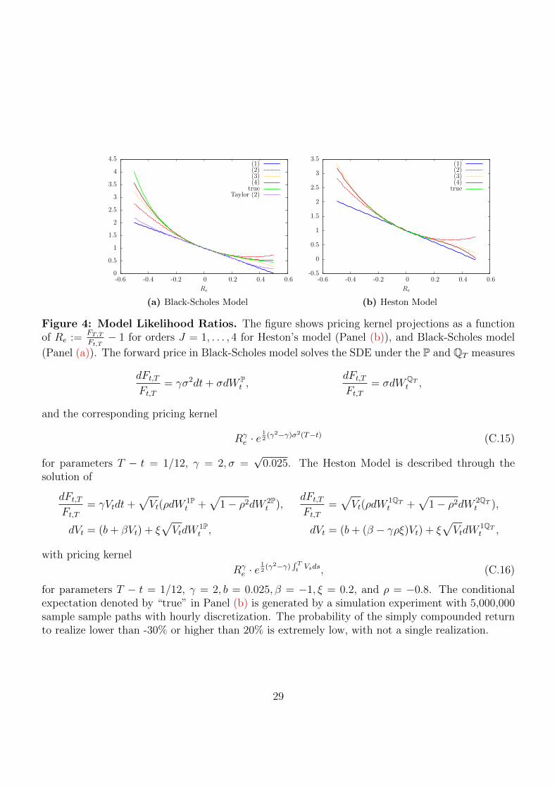
measure which are not measurable with respect to R. We show in Figure 4a

for the Black-Scholes pricing kernel how an order J = 2 likelihood expansion

deviates from a second-order Taylor series expansion. The likelihood expan-

sion ensures for each J that the projection integrates to one, and that the

first J moments of R are perfectly priced. As such it likely converges slower

than a Taylor series expansion. At the same time the economic features of

the LM expansion more than compensate for the slower convergence. We

discuss these issues in more detail in Section 4.4 below. In Figure 4b it can

be seen that the expansion works extremely well already for low orders also

in the presence of stochastic volatility.

The ability to develop an orthonormal basis of order J with respect to

M without knowing explicitly M and Qt,T , just in terms of the moments

µMt,1, . . . , µ

Mt,2J and µQT

t,1 , . . . , µQTt,J , puts us in the position to use our asset pric-

ing bounds in developing the projection. With µQTt,1 , . . . , µ

QTt,J fixed from option

prices, any projection with probability measure M such that the moments

12

satisfy

µPlowert,i ≤ µM

i ≤ µPuppert,i , (16)

is a viable candidate for Pt. To ensure that there exists such a measure we

can use8

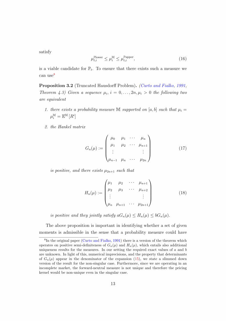
Proposition 3.2 (Truncated Hausdorff Problem). (Curto and Fialko, 1991,

Theorem 4.3) Given a sequence µi, i = 0, . . . , 2n, µi > 0 the following two

are equivalent

1. there exists a probability measure M supported on [a, b] such that µi =

µMi = EM [Ri]

2. the Hankel matrix

Gn(µ) :=

µ0 µ1 · · · µn

µ1 µ2 · · · µn+1

......

µn−1 µn · · · µ2n

(17)

is positive, and there exists µ2n+1 such that

Hn(µ) :=

µ1 µ2 · · · µn+1

µ2 µ3 · · · µn+2

......

µn µn+1 · · · µ2n+1

(18)

is positive and they jointly satisfy aGn(µ) ≤ Hn(µ) ≤ bGn(µ).

The above proposition is important in identifying whether a set of given

moments is admissible in the sense that a probability measure could have

8In the original paper (Curto and Fialko, 1991) there is a version of the theorem whichoperates on positive semi-definiteness of Gn(µ) and Hn(µ), which entails also additionaluniqueness results for the measures. In our setting the required exact values of a and bare unknown. In light of this, numerical imprecisions, and the property that determinantsof Gn(µ) appear in the denominator of the expansion (15), we state a slimmed downversion of the result for the non-singular case. Furthermore, since we are operating in anincomplete market, the forward-neutral measure is not unique and therefore the pricingkernel would be non-unique even in the singular case.

13

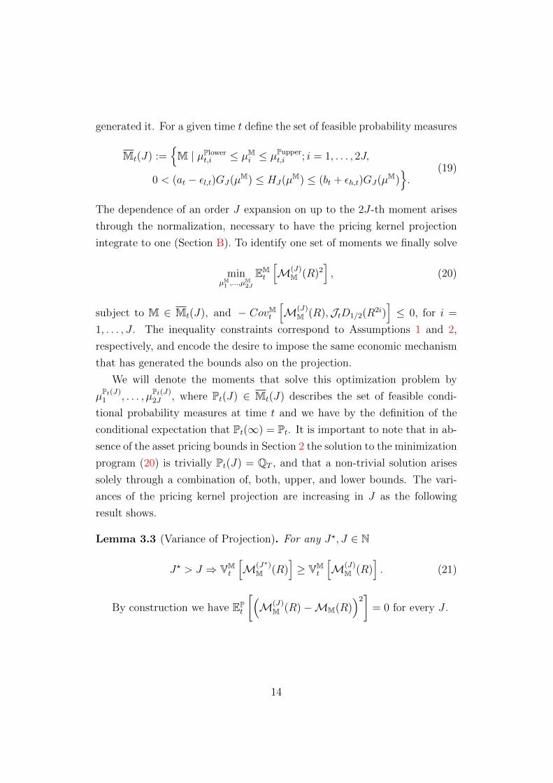
generated it. For a given time t define the set of feasible probability measures

Mt(J) :={M | µPlower

t,i ≤ µMi ≤ µPupper

t,i ; i = 1, . . . , 2J,

0 < (at − εl,t)GJ(µM) ≤ HJ(µM) ≤ (bt + εh,t)GJ(µM)}.

(19)

The dependence of an order J expansion on up to the 2J-th moment arises

through the normalization, necessary to have the pricing kernel projection

integrate to one (Section B). To identify one set of moments we finally solve

minµM1 ,...,µ

M2J

EMt

[M(J)

M (R)2], (20)

subject to M ∈ Mt(J), and − CovMt

[M(J)

M (R),JtD1/2(R2i)]≤ 0, for i =

1, . . . , J . The inequality constraints correspond to Assumptions 1 and 2,

respectively, and encode the desire to impose the same economic mechanism

that has generated the bounds also on the projection.

We will denote the moments that solve this optimization problem by

µPt(J)1 , . . . , µ

Pt(J)2J , where Pt(J) ∈ Mt(J) describes the set of feasible condi-

tional probability measures at time t and we have by the definition of the

conditional expectation that Pt(∞) = Pt. It is important to note that in ab-

sence of the asset pricing bounds in Section 2 the solution to the minimization

program (20) is trivially Pt(J) = QT , and that a non-trivial solution arises

solely through a combination of, both, upper, and lower bounds. The vari-

ances of the pricing kernel projection are increasing in J as the following

result shows.

Lemma 3.3 (Variance of Projection). For any J?, J ∈ N

J? > J ⇒ VMt

[M(J?)

M (R)]≥ VM

t

[M(J)

M (R)]. (21)

By construction we have EPt

[(M(J)

M (R)−MM(R))2]

= 0 for every J .

14

4 Empirical Recovery

We base our empirical studies on a panel of S&P 500 European options in

the sample period from January 1990 to January 2014. Option data are from

MarketDataExpress, a vendor connected to the CBOE. The data set includes

closing bid and ask quotes for each option contract from which we compute

mid prices, along with the corresponding strike price. From the data we filter

out all entries with non-standard settlements and those which violate basic

no-arbitrage conditions. Options mature on the third Friday each month,

and we use this maturity on a monthly time grid to compute forward prices

of divergences. For the same time grid we also use option panels for one

quarter of a year, one half, and a full year. These longer-maturity panels

use interpolation. We replicate time series of forward prices on the S&P

500 spot index using put call parity, consistently with the procedure in the

CBOE (2009) white paper for the computation of the VIX implied volatility

index. In the following Section we describe the behaviour and properties of

the asset pricing bounds implied by the data and Assumptions 1 and 2.

4.1 Realized Conditional Asset Pricing Bounds

In this Section we discuss the empirical implementation and properties of the

bounds developed in Section 2 above. We start by checking empirically the

validity of Assumption 1 unconditionally.9 Unfortunately there is no condi-

tional model-free test, but we can rely on the fact that for a random vari-

able that is positive almost surely (the conditional expectation in question),

also its unconditional expectation will be positive. A sample average that

supports the assumptions with high probability unconditionally is therefore

evidence that the assumptions may also hold conditionally. For this purpose

we compute averages of excess returns on realized divergence using decompo-

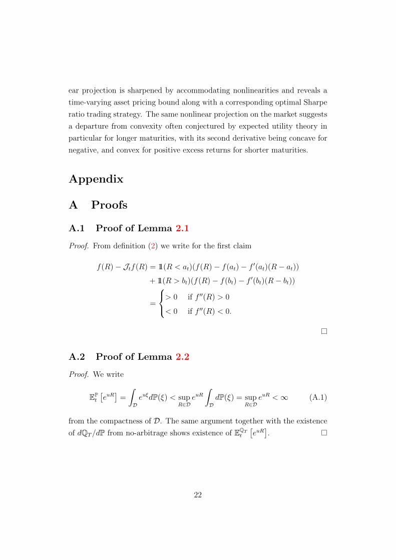
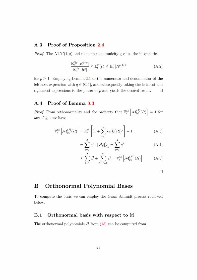
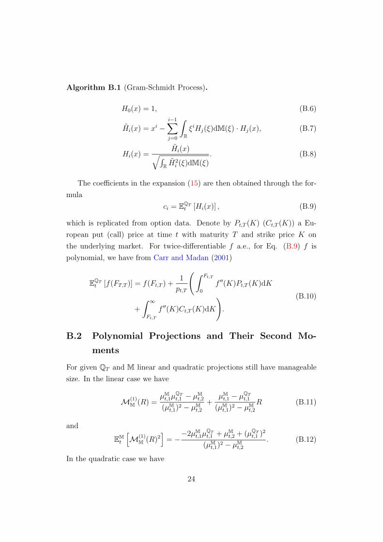
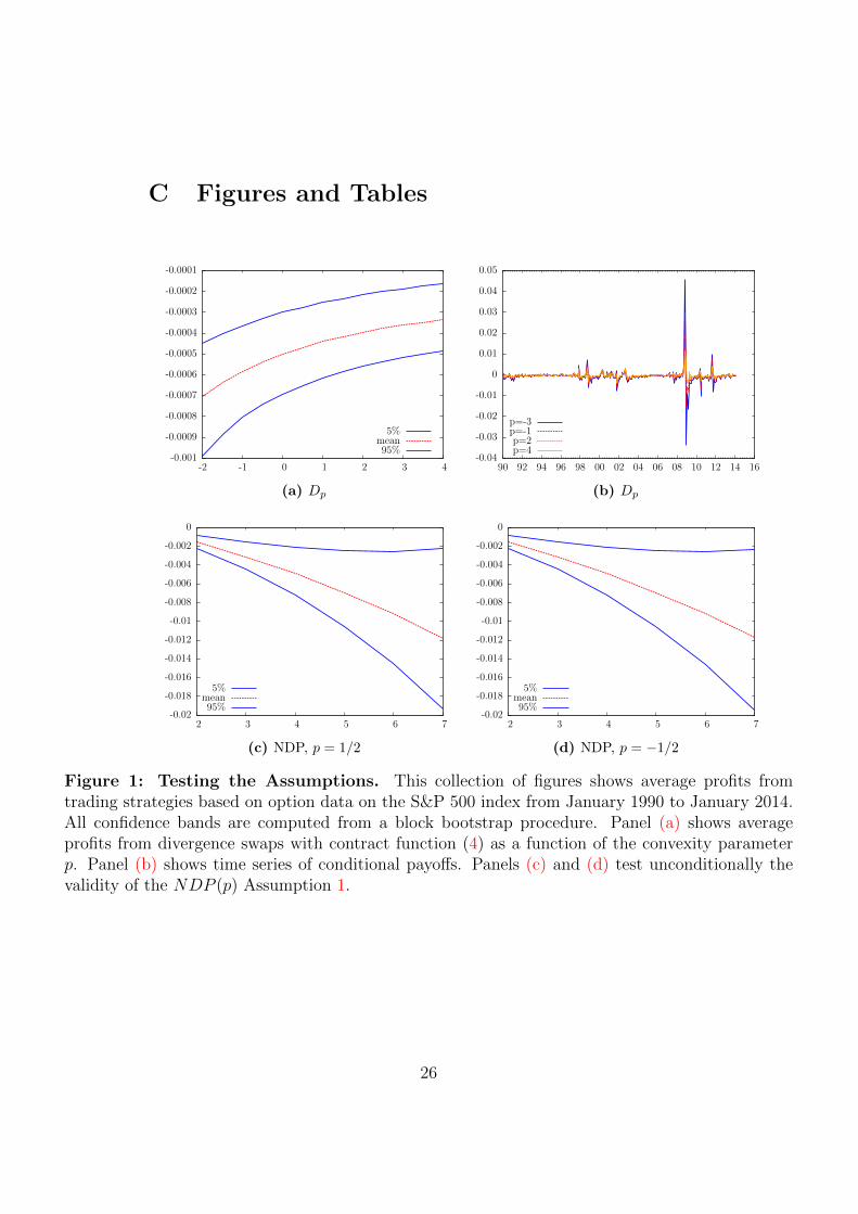
sition (6). Figure 1 shows summary statistics of this decomposition. In the

first Panel 1a we see that unconditionally it is profitable to sell divergence

swaps uniformly across different p. This result is known already from Schnei-

9For Assumption 2 we rely on the tests performed in Martin (2015).

15

der and Trojani (2015) along with the fact that conditionally, excess returns

from different divergence swaps co-move (Panel 1b). Panels 1c and 1d sug-

gest that Assumption 1 appears reasonable. Independently of the convexity

parameter p, divergence swaps on powers of the S&P 500 lose money. With

high probability the unconditional premium is negative, making it conceiv-

able that this is valid also for the conditional one. Martin (2015) provides

empirical and theoretical evidence for the validity of the NCC(1, 1). Upon

accepting the empirical validation of the theoretical assumptions we can now

move on to their implications.10

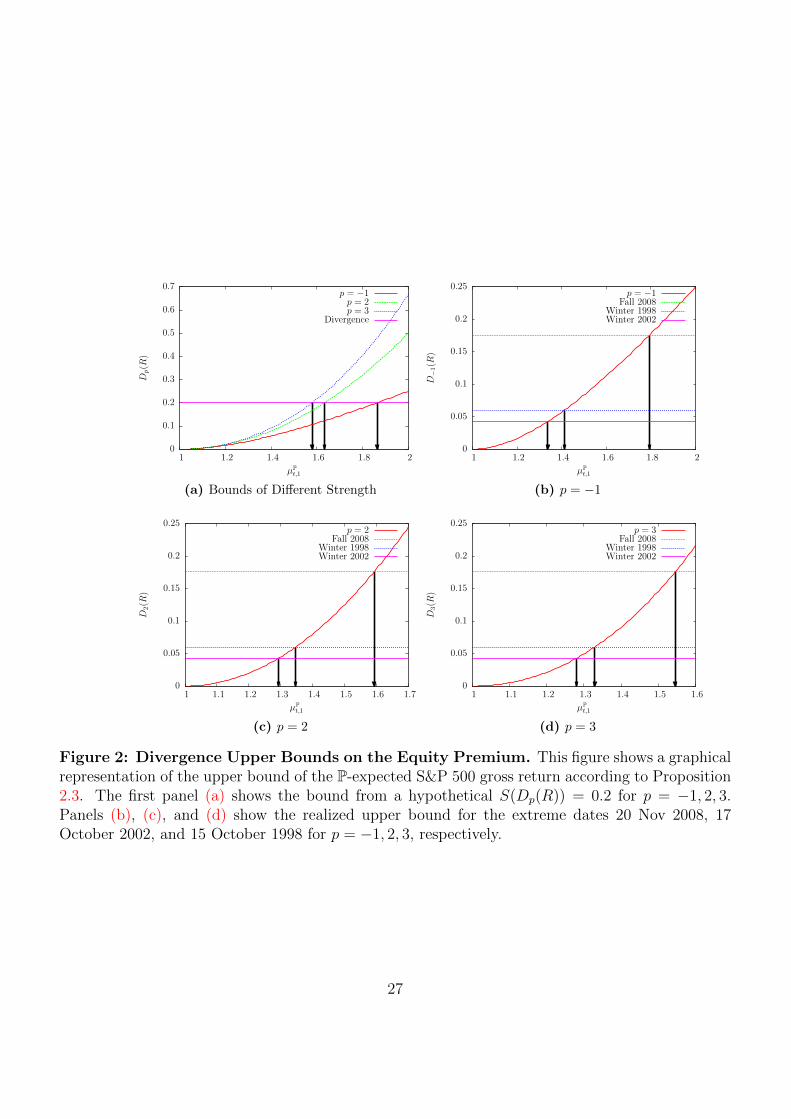
Figure 2a indicates how the choice of parameter p determines the tight-

ness of the upper bound considerably. In particular at crisis dates, Panels

2b, 2c, and 2d show differences of up to 50% between bounds of different

strength. Over time the bounds of various strength are time-varying and

they never overlap (Figure 3a). A similar behavior can be seen also for the

lower bounds in panel 3b. There is a time-consistent ranking between the

bounds determined by the parameter q. This consistency is also between

upper and lower bounds. Putting lower and upper bounds together Figure

3c shows a band in which the equity premium can be locked in. There is con-

siderable time variation in the difference between upper and lower bounds

(Figure 3d). Out of all available parametrizations we continue our analysis

using p = 1/2 for the upper bounds exclusively, and q = 1 for the lower

bounds in connection with Proposition 2.4, respectively, for simplicity, to

conform with the prevailing literature, and in light of the applications to

come. In the next Section we make use of the asset pricing bounds described

above to guide our search for a family of conditional probability measures.

4.2 An (Almost) Model-Free Projection

For every third Friday each month from January 1990 to January 2014 we

solve the optimization program (20) for J = 1, 2, 3 for the maturities 1, 3, 6,

and 12 months. This task may numerically become challenging in particular

10If the assumptions do not seem reasonable on a given day, the researcher has thefreedom to refrain from using the bounds, or employ them with even more conservativeparameters.

16

for higher-order expansions in that the Hankel matrix (17) may only be

barely positive, with the computation being subject to numerical imprecisions

through adding very large to very small numbers.11 The objective function

is highly nonlinear in the moments, and with the additional burden of highly

nonlinear constraints we minimize using the Bayesian MCMC method from

Chernozhukov and Hong (2003). There are certain dates for which there

is no feasible parameter constellation, for instance when the Hankel matrix

of the QT moments is not positive, or the constraints leave only an empty

set, in which case we skip the projection for that day and do not record

implied Pt(J) moments. We perform the minimization in terms of gross

moments. After obtaining µPt(J) we convert them into simply compounded

moments µPt(J)e by adding and subtracting the gross moments according to

the binomial formula. We obtain gross moments separately for each order J .

Gross moments are numerically very close for each J , suggesting that µPt(1)

could be reused for the computation of µPt(2) and so forth, but the constraints

are too stringent too allow for this recursive program.

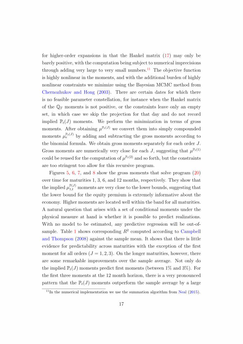
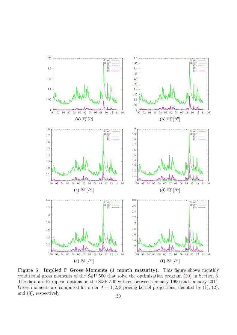
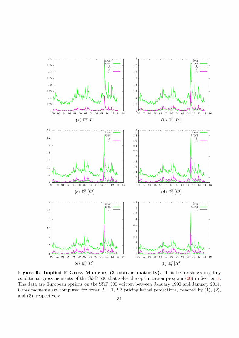
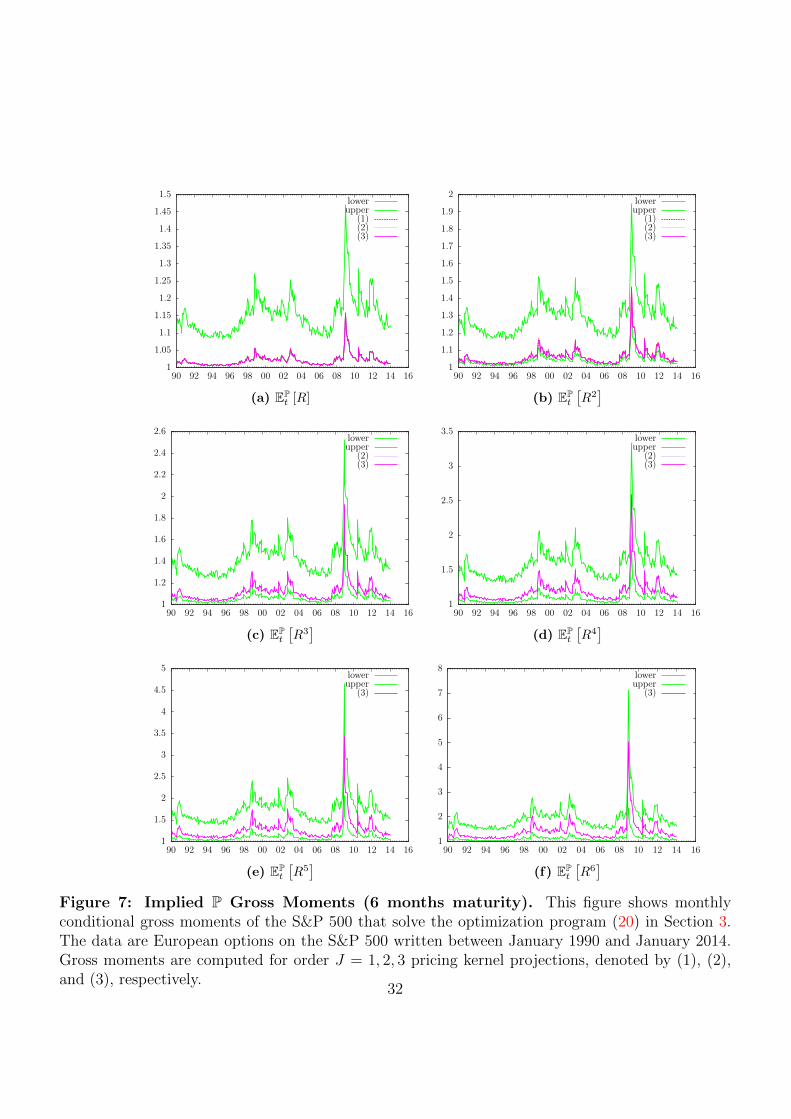
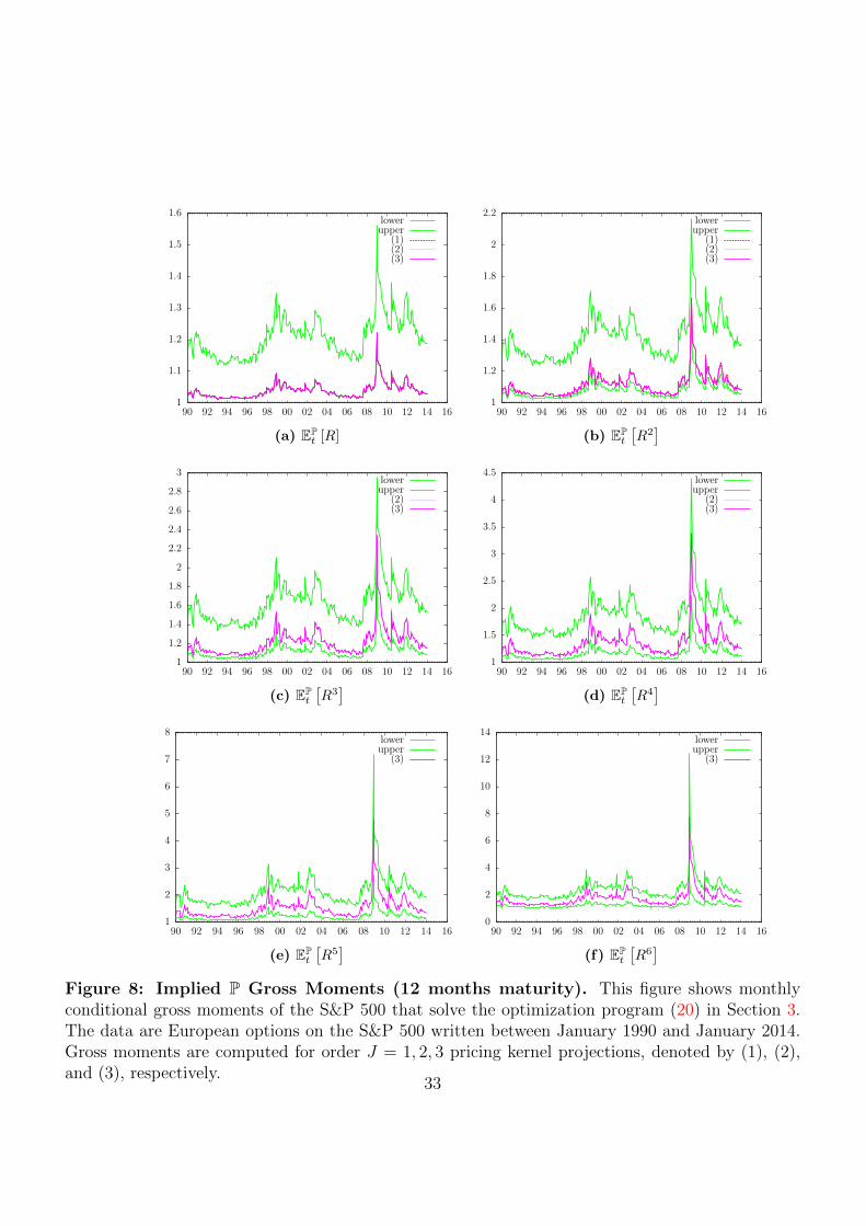
Figures 5, 6, 7, and 8 show the gross moments that solve program (20)

over time for maturities 1, 3, 6, and 12 months, respectively. They show that

the implied µP(J)1,t moments are very close to the lower bounds, suggesting that

the lower bound for the equity premium is extremely informative about the

economy. Higher moments are located well within the band for all maturities.

A natural question that arises with a set of conditional moments under the

physical measure at hand is whether it is possible to predict realizations.

With no model to be estimated, any predictive regression will be out-of-

sample. Table 1 shows corresponding R2 computed according to Campbell

and Thompson (2008) against the sample mean. It shows that there is little

evidence for predictability across maturities with the exception of the first

moment for all orders (J = 1, 2, 3). On the longer maturities, however, there

are some remarkable improvements over the sample average. Not only do

the implied Pt(J) moments predict first moments (between 1% and 3%). For

the first three moments at the 12 month horizon, there is a very pronounced

pattern that the Pt(J) moments outperform the sample average by a large

11In the numerical implementation we use the summation algorithm from Neal (2015).

17

margin.

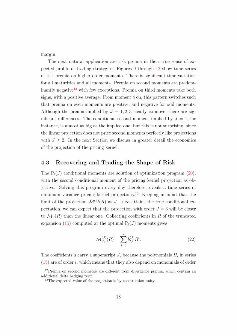
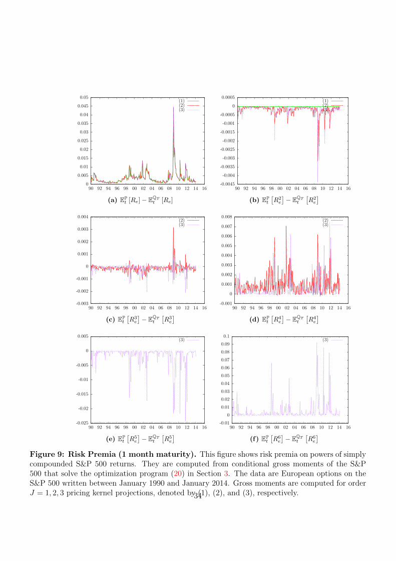
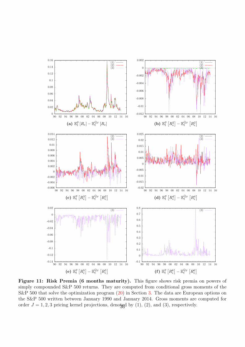
The next natural application are risk premia in their true sense of ex-

pected profits of trading strategies. Figures 9 through 12 show time series

of risk premia on higher-order moments. There is significant time variation

for all maturities and all moments. Premia on second moments are predom-

inantly negative12 with few exceptions. Premia on third moments take both

signs, with a positive average. From moment 4 on, this pattern switches such

that premia on even moments are positive, and negative for odd moments.

Although the premia implied by J = 1, 2, 3 clearly co-move, there are sig-

nificant differences. The conditional second moment implied by J = 1, for

instance, is almost as big as the implied one, but this is not surprising, since

the linear projection does not price second moments perfectly like projections

with J ≥ 2. In the next Section we discuss in greater detail the economics

of the projection of the pricing kernel.

4.3 Recovering and Trading the Shape of Risk

The Pt(J) conditional moments are solution of optimization program (20),

with the second conditional moment of the pricing kernel projection as ob-

jective. Solving this program every day therefore reveals a time series of

minimum variance pricing kernel projections.13 Keeping in mind that the

limit of the projection M(J)(R) as J → ∞ attains the true conditional ex-

pectation, we can expect that the projection with order J = 3 will be closer

to MP(R) than the linear one. Collecting coefficients in R of the truncated

expansion (15) computed at the optimal Pt(J) moments gives

M(J)Pt

(R) =J∑i=0

b(J)t,i R

i. (22)

The coefficients a carry a superscript J , because the polynomials Hi in series

(15) are of order i, which means that they also depend on monomials of order

12Premia on second moments are different from divergence premia, which contain anadditional delta hedging term.

13The expected value of the projection is by construction unity.

18

j ≤ i. This in turn means that b(J)t,i will in general be different from b

(K)t,i if

K 6= J . In fact, a small change between b(J)t,i and b

(J+1)t,i indicates convergence,

since contributions from higher-order moments do not change the projection

any more. While it is also to be expected that CovPt (Rn, Rm) > 0 for any

n,m ≥ 1, the coefficients b(J)t,i of the expansion can take both negative and

positive signs. We investigate this in greater detail in Section 4.4 below.

From Proposition 3.3 we know however a-priori that the conditional second

moment of the projection will be increasing in J .14 We can also easily convert

from moments of gross returns to moments of discrete returns Re := R − 1

by using the binomial formula, recomputing the basis and re-collecting the

coefficients

M(J)Pt

(Re) =J∑i=0

a(J)t,i R

ie. (23)

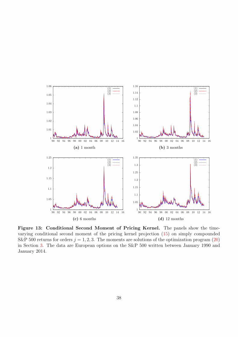
Figure 13 reveals the corresponding sample paths, and suggests that em-

pirically the variance is indeed greater for higher-order expansions. While

for 1 month maturity the second moments are almost identical, the differ-

ences widen substantially with maturity, however. The trajectories of the

linear projection in Panel 13a, 13b, 13c, and 13d correspond to time-varying

Hansen-Jagannathan bounds for multiple maturities, while the ones for the

higher-order projections correspond to nonlinear extensions which are likely

closer to the true, unobserved projection.

From Schneider (2015) we know that there is also a tradeable aspect

of this. Since we can replicate through options contracts on Rie, the same is

possible also for weighted sums thereof. The expected profit of the projection

is minus the variance of the pricing kernel. Table 2 gives the corresponding

sample averages, which correspond roughly to the minus the kernel projection

second moments in Figure 13 plus 1.

14This result holds if the first 2(J − 1) moments of the order J projection are equal tothe ones of the order J − 1 projection. This is not the case in general, but the moments ofthe different-order projections are sufficiently close together to justify a rough comparison.

19

4.4 Risk Aversion

In this Section we compare our projection to extant expected utility models.

Taking recourse to a representative agent economy, we can write a pricing

kernel in terms of the wealth of the agent (see, for example Garcia et al.,

2009) as

MEU =U ′(Wt+1)

U ′(Wt), (24)

where EU denotes expected utility and U a Von-Neumann Morgenstern con-

cave utility function. An expansion of the above around Wt and denoting by

REUe := Wt+1

Wt− 1 we have for instance to order 2

MEU = 1 +WtU ′′(Wt)

U ′(Wt)REUe +W 2

t

U ′′′(Wt)

U ′(Wt)

(REUe

)2+O

(REUe

)3. (25)

From the concavity of U it follows that WtU ′′(Wt)U ′(Wt)

< 0 and W 2tU ′′′(Wt)U ′(Wt)

> 0.

The former sign is associated with aversion to uncertainty, while the latter

is associated with prudence of the representative agent and the signs con-

tinue alternating in the same manner for higher-order terms. Before turn-

ing to comparing the coefficients of our projection to the coefficients of the

Taylor expansion above we gauge signs and magnitudes from well-known no-

arbitrage models. Indeed Black-Scholes model for the same parametrizations

as in Figure 4a exhibits these signs, negative for odd orders, and positive

for even. Heston’s model with the same parameters that generated 4b on

the other hand features a negative coefficient in an order four expansion on

the coefficient on R2e. It is therefore conceivable that signs and magnitudes

may be subject to additional risk factors. In the case of Heston’s model it is

stochastic volatility (see also the discussion in Chabi-Yo et al., 2008; Hansen

and Renault, 2010).

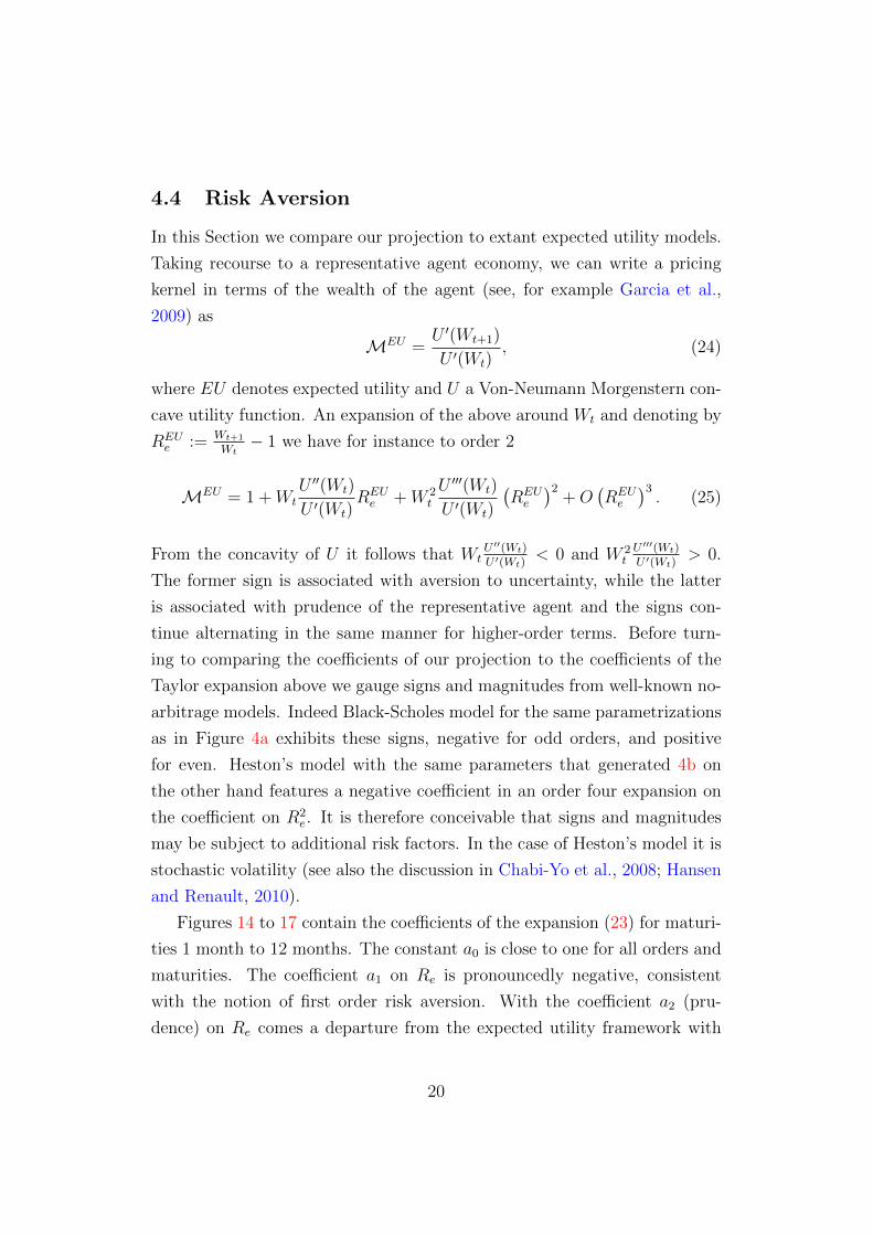
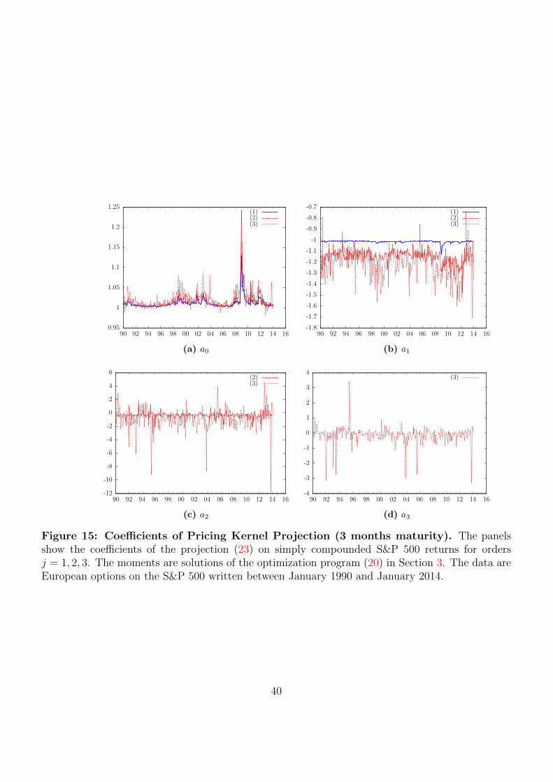
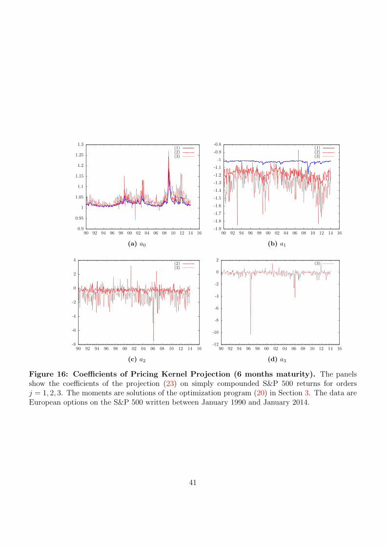
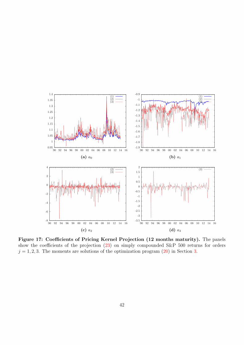
Figures 14 to 17 contain the coefficients of the expansion (23) for maturi-

ties 1 month to 12 months. The constant a0 is close to one for all orders and

maturities. The coefficient a1 on Re is pronouncedly negative, consistent

with the notion of first order risk aversion. With the coefficient a2 (pru-

dence) on Re comes a departure from the expected utility framework with

20

Re-measurable pricing kernels. It is close to zero, but takes on large positive

and negative values over time. With an increase in maturity it becomes neg-

ative on average and less variable. With the coefficient a3 a similar pattern

evolves, albeit much less pronounced, taking negative and positive values

on average close to zero for all maturities. With a lot of time variation in

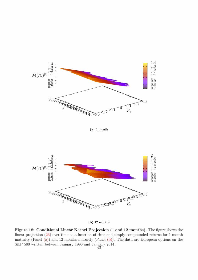
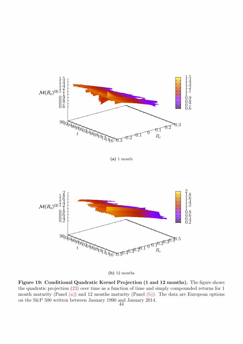
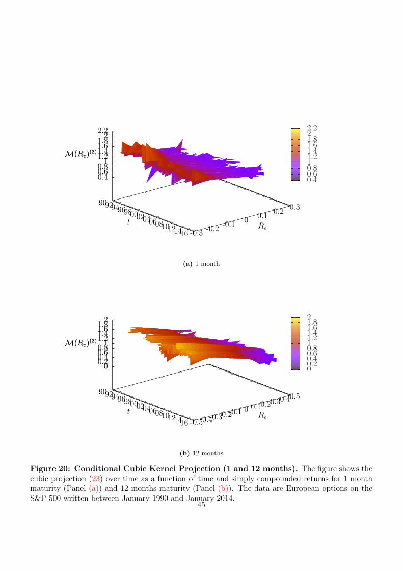
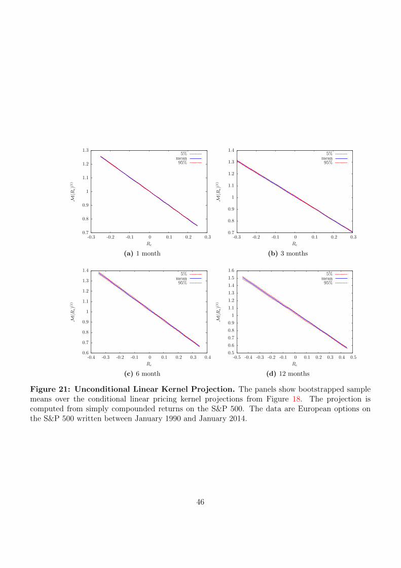
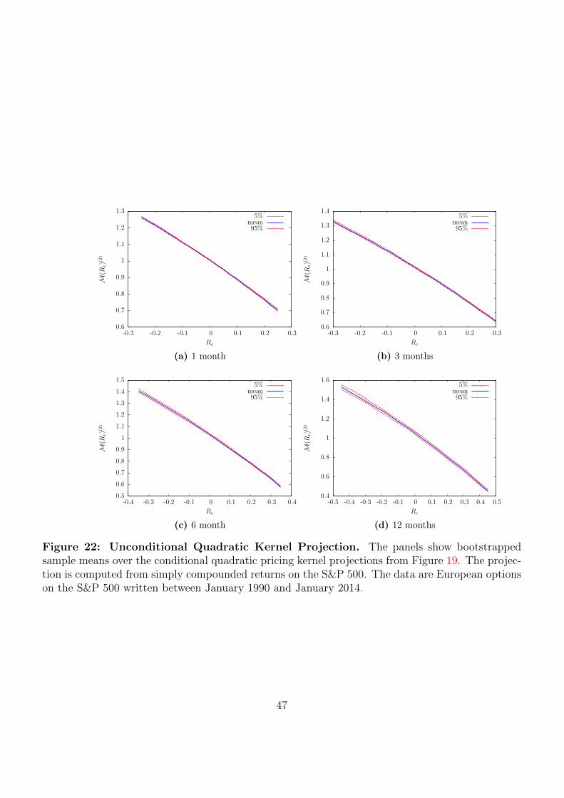
the coefficients, Figures 18 to 20b show a rich variety of different shapes of

the pricing kernel over time. The quadratic projection on average suggests a

concave shape (Figure 22). This situation changes once one considers a cubic

projection, which is concave for negative and convex for positive returns at 1

month maturity, while it appears to be globally concave for longer maturities.

5 Conclusion

This paper develops a set of conditional lower and upper bounds for expected

powers of gross market returns from an assumption about the sign of expected

payoffs from certain contracts. The assumptions can be empirically tested

and are valid at least on average. The bounds determine a set of possible

conditional physical probability measures, the size of which we further re-

duce by picking a family of moments which minimizes the second moment of

a projection of the pricing kernel analogously to the notion of minimum vari-

ance martingale measures in incomplete markets. The resulting conditional

moments recover families of physical probability measures solely on the basis

of the economic assumptions generating the bounds, but do not make as-

sumptions about Markovianity, stationarity, or the type of stochastic process

driving the economy. They yield a number of novel economic insights. The

lower bounds on the equity premium are extremely informative for all higher-

order physical moments and hence the physical conditional distribution. In

light of the consistency conditions between moments of different orders this

means that the lower bound for the first moment, the equity premium, is

of paramount importance. Upper bounds establish relations between phys-

ical and forward-neutral moments jointly and put additional structure on

the pricing kernel. The resulting conditional moments predict realizations

out-of-sample. The traditional Hansen-Jagannathan bound based on a lin-

21

ear projection is sharpened by accommodating nonlinearities and reveals a

time-varying asset pricing bound along with a corresponding optimal Sharpe

ratio trading strategy. The same nonlinear projection on the market suggests

a departure from convexity often conjectured by expected utility theory in

particular for longer maturities, with its second derivative being concave for

negative, and convex for positive excess returns for shorter maturities.

Appendix

A Proofs

A.1 Proof of Lemma 2.1

Proof. From definition (2) we write for the first claim

f(R)− Jtf(R) = 11(R < at)(f(R)− f(at)− f ′(at)(R− at))

+ 11(R > bt)(f(R)− f(bt)− f ′(bt)(R− bt))

=

> 0 if f ′′(R) > 0

< 0 if f ′′(R) < 0.


Proof. We write

EPt

[euR]

=

∫DeuξdP(ξ) < sup

R∈DeuR

∫DdP(ξ) = sup

R∈DeuR <∞ (A.1)

from the compactness of D. The same argument together with the existence

of dQT/dP from no-arbitrage shows existence of EQTt

[euR].

22

A.3 Proof of Proposition 2.4

Proof. The NCC(1, q) and moment monotonicity give us the inequalities

EQTt [R1+q]

EQTt [Rq]

≤ EPt [R] ≤ EP

t [Rp]1/p (A.2)

for p ≥ 1. Employing Lemma 2.1 to the numerator and denominator of the

leftmost expression with q ∈ (0, 1], and subsequently taking the leftmost and

rightmost expressions to the power of p and yields the desired result.


Proof. From orthonormality and the property that EMt

[M(J)

M (R)]

= 1 for

any J ≥ 1 we have

VMt

[M(J)

M (R)]

= EMt

[(1 +

J∑i=1

ciHi(R))2

]− 1 (A.3)

=J∑i=1

c2i · ‖Hi‖2L2M =J∑i=1

c2i (A.4)

≤J∑i=1

c2i +J?∑

i=J+1

c2i = VMt

[M(J?)

M (R)]

(A.5)

B Orthonormal Polynomial Bases

To compute the basis we can employ the Gram-Schmidt process reviewed

below.

B.1 Orthonormal basis with respect to M

The orthonormal polynomials H from (15) can be computed from

23

Algorithm B.1 (Gram-Schmidt Process).

H0(x) = 1, (B.6)

Hi(x) = xi −i−1∑j=0

∫RξiHj(ξ)dM(ξ) ·Hj(x), (B.7)

Hi(x) =Hi(x)√∫

R H2i (ξ)dM(ξ)

. (B.8)

The coefficients in the expansion (15) are then obtained through the for-

mula

ci = EQTt [Hi(x)] , (B.9)

which is replicated from option data. Denote by Pt,T (K) (Ct,T (K)) a Eu-

ropean put (call) price at time t with maturity T and strike price K on

the underlying market. For twice-differentiable f a.e., for Eq. (B.9) f is

polynomial, we have from Carr and Madan (2001)

EQTt [f(FT,T )] = f(Ft,T ) +

1

pt,T

(∫ Ft,T

0

f ′′(K)Pt,T (K)dK

+

∫ ∞Ft,T

f ′′(K)Ct,T (K)dK

).

(B.10)

B.2 Polynomial Projections and Their Second Mo-

ments

For given QT and M linear and quadratic projections still have manageable

size. In the linear case we have

M(1)M (R) =

µMt,1µ

QTt,1 − µM

t,2

(µMt,1)

2 − µMt,2

+µMt,1 − µ

QTt,1

(µMt,1)

2 − µMt,2

R (B.11)

and

EMt

[M(1)

M (R)2]

= −−2µM

t,1µQTt,1 + µM

t,2 + (µQTt,1 )2

(µMt,1)

2 − µMt,2

. (B.12)

In the quadratic case we have

24

M(2)M (R) =

−µMt,3(µ

Mt,1µ

QTt,2 + µM

t,2µQTt,1 ) + µM

t,1µMt,4µ

QTt,1 + (µM

t,2)2µQT

t,2 − µMt,2µ

Mt,4 + (µM

t,3)2

(µMt,1)

2µMt,4 − µM

t,2(2µMt,1µ

Mt,3 + µM

t,4) + (µMt,2)

3 + (µMt,3)

2

+−µM

t,2(µMt,1µ

QTt,2 + µM

t,3) + µMt,4(µ

Mt,1 − µ

QTt,1 ) + (µM

t,2)2µQT

t,1 + µMt,3µ

QTt,2

(µMt,1)

2µMt,4 − µM

t,2(2µMt,1µ

Mt,3 + µM

t,4) + (µMt,2)

3 + (µMt,3)

2R

+(µM

t,1)2µQT

t,2 − µMt,2(µ

Mt,1µ

QTt,1 + µQT

t,2 )− µMt,1µ

Mt,3 + (µM

t,2)2 + µM

t,3µQTt,1

(µMt,1)

2µMt,4 − µM

t,2(2µMt,1µ

Mt,3 + µM

t,4) + (µMt,2)

3 + (µMt,3)

2R2

(B.13)

and

EMt

[M(2)

M (R)2]

=1

(µMt,1)

2µMt,4 − µM

t,2(2µMt,1µ

Mt,3 + µM

t,4) + (µMt,2)

3 + (µMt,3)

2

·

((µM

t,1)2(µQT

t,2 )2 − 2µMt,3(µ

QTt,2 (µM

t,1 − µQTt,1 ) + µM

t,2µQTt,1 )

− µMt,2

(2µM

t,1µQTt,1 µ

QTt,2 + µM

t,4 + (µQTt,2 )2

)+ µM

t,4µQTt,1 (2µM

t,1 − µQTt,1 )

+ (µMt,2)

2((µQT

t,1 )2 + 2µQTt,2

)+ (µM

t,3)2

).

(B.14)

25

C Figures and Tables

-0.001

-0.0009

-0.0008

-0.0007

-0.0006

-0.0005

-0.0004

-0.0003

-0.0002

-0.0001

-2 -1 0 1 2 3 4

5%mean95%

(a) Dp

-0.04

-0.03

-0.02

-0.01

0

0.01

0.02

0.03

0.04

0.05

90 92 94 96 98 00 02 04 06 08 10 12 14 16

p=-3p=-1p=2p=4

(b) Dp

-0.02

-0.018

-0.016

-0.014

-0.012

-0.01

-0.008

-0.006

-0.004

-0.002

0

2 3 4 5 6 7

5%mean95%

(c) NDP, p = 1/2

-0.02

-0.018

-0.016

-0.014

-0.012

-0.01

-0.008

-0.006

-0.004

-0.002

0

2 3 4 5 6 7

5%mean95%

(d) NDP, p = −1/2

Figure 1: Testing the Assumptions. This collection of figures shows average profits fromtrading strategies based on option data on the S&P 500 index from January 1990 to January 2014.All confidence bands are computed from a block bootstrap procedure. Panel (a) shows averageprofits from divergence swaps with contract function (4) as a function of the convexity parameterp. Panel (b) shows time series of conditional payoffs. Panels (c) and (d) test unconditionally thevalidity of the NDP (p) Assumption 1.

26

0

0.1

0.2

0.3

0.4

0.5

0.6

0.7

1 1.2 1.4 1.6 1.8 2

Dp(R

)

µPt,1

p = −1p = 2p = 3

Divergence

(a) Bounds of Different Strength

0

0.05

0.1

0.15

0.2

0.25

1 1.2 1.4 1.6 1.8 2

D−1(R

)

µPt,1

p = −1Fall 2008

Winter 1998Winter 2002

(b) p = −1

0

0.05

0.1

0.15

0.2

0.25

1 1.1 1.2 1.3 1.4 1.5 1.6 1.7

D2(R

)

µPt,1

p = 2Fall 2008


(c) p = 2

0

0.05

0.1

0.15

0.2

0.25

1 1.1 1.2 1.3 1.4 1.5 1.6

D3(R

)

µPt,1

p = 3Fall 2008


(d) p = 3

Figure 2: Divergence Upper Bounds on the Equity Premium. This figure shows a graphicalrepresentation of the upper bound of the P-expected S&P 500 gross return according to Proposition2.3. The first panel (a) shows the bound from a hypothetical S(Dp(R)) = 0.2 for p = −1, 2, 3.Panels (b), (c), and (d) show the realized upper bound for the extreme dates 20 Nov 2008, 17October 2002, and 15 October 1998 for p = −1, 2, 3, respectively.

27

0.1

0.2

0.3

0.4

0.5

0.6

0.7

0.8

90 92 94 96 98 00 02 04 06 08 10 12 14

p = −1p = 0.5p = 2p = 3p = 4

(a) Upper Bounds

0

0.05

0.1

0.15

0.2

0.25

0.3

0.35

0.4

0.45

0.5

90 92 94 96 98 00 02 04 06 08 10 12 14 16

q = 3q = 2q = 1

q = 0.5q = 0.1

(b) Lower Bounds

0

0.05

0.1

0.15

0.2

0.25

0.3

0.35

0.4

0.45

90 92 94 96 98 00 02 04 06 08 10 12 14 16

Equity Premium Band

(c) Admissible Region

0.08

0.1

0.12

0.14

0.16

0.18

0.2

0.22

90 92 94 96 98 00 02 04 06 08 10 12 14 16

(d) Difference Between Bounds

Figure 3: Divergence Upper and Lower Bounds on the Equity Premium. The figureshows upper (a) bounds from Proposition 2.3 for n = 1 and different p, and lower (b) bounds fromProposition 2.4 on the S&P 500 equity premium for p = 1 and different choices of q. Panel (c)shows the admissible region implied by the lower bound with p = 1 and q = 1, and the upper boundimplied by p = 2 in annualized percentage terms. Panel (d) shows the difference between the upperand the lower bound from panel (c). The sample period ranges from January 1990 to January 2014and the data are European options on the S&P 500 index.

28

0

0.5

1

1.5

2

2.5

3

3.5

4

4.5

-0.6 -0.4 -0.2 0 0.2 0.4 0.6

Re

(1)(2)(3)(4)

trueTaylor (2)

(a) Black-Scholes Model

-0.5

0

0.5

1

1.5

2

2.5

3

3.5

-0.6 -0.4 -0.2 0 0.2 0.4 0.6

Re

(1)(2)(3)(4)

true

(b) Heston Model

Figure 4: Model Likelihood Ratios. The figure shows pricing kernel projections as a functionof Re :=

FT,T

Ft,T− 1 for orders J = 1, . . . , 4 for Heston’s model (Panel (b)), and Black-Scholes model

(Panel (a)). The forward price in Black-Scholes model solves the SDE under the P and QT measures

dFt,TFt,T

= γσ2dt+ σdW Pt ,

dFt,TFt,T

= σdWQTt ,

and the corresponding pricing kernel

Rγe · e

12(γ2−γ)σ2(T−t) (C.15)

for parameters T − t = 1/12, γ = 2, σ =√

0.025. The Heston Model is described through thesolution of

dFt,TFt,T

= γVtdt+√Vt(ρdW

1Pt +

√1− ρ2dW 2P

t ),dFt,TFt,T

=√Vt(ρdW

1QTt +

√1− ρ2dW 2QT

t ),

dVt = (b+ βVt) + ξ√VtdW

1Pt , dVt = (b+ (β − γρξ)Vt) + ξ

√VtdW

1QTt ,

with pricing kernel

Rγe · e

12(γ2−γ)

∫ Tt Vsds, (C.16)

for parameters T − t = 1/12, γ = 2, b = 0.025, β = −1, ξ = 0.2, and ρ = −0.8. The conditionalexpectation denoted by “true” in Panel (b) is generated by a simulation experiment with 5,000,000sample sample paths with hourly discretization. The probability of the simply compounded returnto realize lower than -30% or higher than 20% is extremely low, with not a single realization.

29

1

1.05

1.1

1.15

1.2

1.25

90 92 94 96 98 00 02 04 06 08 10 12 14 16

lowerupper

(1)(2)(3)

(a) EPt [R]

1

1.05

1.1

1.15

1.2

1.25

1.3

1.35

1.4

1.45

1.5

90 92 94 96 98 00 02 04 06 08 10 12 14 16

lowerupper

(1)(2)(3)

(b) EPt

[R2]

1

1.1

1.2

1.3

1.4

1.5

1.6

1.7

1.8

90 92 94 96 98 00 02 04 06 08 10 12 14 16

lowerupper

(2)(3)

(c) EPt

[R3] 1

1.1

1.2

1.3

1.4

1.5

1.6

1.7

1.8

1.9

2

90 92 94 96 98 00 02 04 06 08 10 12 14 16

lowerupper

(2)(3)

(d) EPt

[R4]

1

1.2

1.4

1.6

1.8

2

2.2

2.4

90 92 94 96 98 00 02 04 06 08 10 12 14 16

lowerupper

(3)

(e) EPt

[R5] 1

1.2

1.4

1.6

1.8

2

2.2

2.4

2.6

2.8

90 92 94 96 98 00 02 04 06 08 10 12 14 16

lowerupper

(3)

(f) EPt

[R6]

Figure 5: Implied P Gross Moments (1 month maturity). This figure shows monthlyconditional gross moments of the S&P 500 that solve the optimization program (20) in Section 3.The data are European options on the S&P 500 written between January 1990 and January 2014.Gross moments are computed for order J = 1, 2, 3 pricing kernel projections, denoted by (1), (2),and (3), respectively.

30

1

1.05

1.1

1.15

1.2

1.25

1.3

1.35

1.4

90 92 94 96 98 00 02 04 06 08 10 12 14 16

lowerupper

(1)(2)(3)

(a) EPt [R]

1

1.1

1.2

1.3

1.4

1.5

1.6

1.7

1.8

90 92 94 96 98 00 02 04 06 08 10 12 14 16

lowerupper

(1)(2)(3)

(b) EPt

[R2]

1

1.2

1.4

1.6

1.8

2

2.2

2.4

90 92 94 96 98 00 02 04 06 08 10 12 14 16

lowerupper

(2)(3)

(c) EPt

[R3] 1

1.2

1.4

1.6

1.8

2

2.2

2.4

2.6

2.8

3

90 92 94 96 98 00 02 04 06 08 10 12 14 16

lowerupper

(2)(3)

(d) EPt

[R4]

1

1.5

2

2.5

3

3.5

4

90 92 94 96 98 00 02 04 06 08 10 12 14 16

lowerupper

(3)

(e) EPt

[R5] 1

1.5

2

2.5

3

3.5

4

4.5

5

5.5

90 92 94 96 98 00 02 04 06 08 10 12 14 16

lowerupper

(3)

(f) EPt

[R6]

Figure 6: Implied P Gross Moments (3 months maturity). This figure shows monthlyconditional gross moments of the S&P 500 that solve the optimization program (20) in Section 3.The data are European options on the S&P 500 written between January 1990 and January 2014.Gross moments are computed for order J = 1, 2, 3 pricing kernel projections, denoted by (1), (2),and (3), respectively.

31

1

1.05

1.1

1.15

1.2

1.25

1.3

1.35

1.4

1.45

1.5

90 92 94 96 98 00 02 04 06 08 10 12 14 16

lowerupper

(1)(2)(3)

(a) EPt [R]

1

1.1

1.2

1.3

1.4

1.5

1.6

1.7

1.8

1.9

2

90 92 94 96 98 00 02 04 06 08 10 12 14 16

lowerupper

(1)(2)(3)

(b) EPt

[R2]

1

1.2

1.4

1.6

1.8

2

2.2

2.4

2.6

90 92 94 96 98 00 02 04 06 08 10 12 14 16

lowerupper

(2)(3)

(c) EPt

[R3] 1

1.5

2

2.5

3

3.5

90 92 94 96 98 00 02 04 06 08 10 12 14 16

lowerupper

(2)(3)

(d) EPt

[R4]

1

1.5

2

2.5

3

3.5

4

4.5

5

90 92 94 96 98 00 02 04 06 08 10 12 14 16

lowerupper

(3)

(e) EPt

[R5] 1

2

3

4

5

6

7

8

90 92 94 96 98 00 02 04 06 08 10 12 14 16

lowerupper

(3)

(f) EPt

[R6]


32

1

1.1

1.2

1.3

1.4

1.5

1.6

90 92 94 96 98 00 02 04 06 08 10 12 14 16

lowerupper

(1)(2)(3)

(a) EPt [R]

1

1.2

1.4

1.6

1.8

2

2.2

90 92 94 96 98 00 02 04 06 08 10 12 14 16

lowerupper

(1)(2)(3)

(b) EPt

[R2]

1

1.2

1.4

1.6

1.8

2

2.2

2.4

2.6

2.8

3

90 92 94 96 98 00 02 04 06 08 10 12 14 16

lowerupper

(2)(3)

(c) EPt

[R3] 1

1.5

2

2.5

3

3.5

4

4.5

90 92 94 96 98 00 02 04 06 08 10 12 14 16

lowerupper

(2)(3)

(d) EPt

[R4]

1

2

3

4

5

6

7

8

90 92 94 96 98 00 02 04 06 08 10 12 14 16

lowerupper

(3)

(e) EPt

[R5] 0

2

4

6

8

10

12

14

90 92 94 96 98 00 02 04 06 08 10 12 14 16

lowerupper

(3)

(f) EPt

[R6]


33

0

0.005

0.01

0.015

0.02

0.025

0.03

0.035

0.04

0.045

0.05

90 92 94 96 98 00 02 04 06 08 10 12 14 16

(1)(2)(3)

(a) EPt [Re]− EQT

t [Re]

-0.0045

-0.004

-0.0035

-0.003

-0.0025

-0.002

-0.0015

-0.001

-0.0005

0

0.0005

90 92 94 96 98 00 02 04 06 08 10 12 14 16

(1)(2)(3)

(b) EPt

[R2

e

]− EQT

t

[R2

e

]

-0.003

-0.002

-0.001

0

0.001

0.002

0.003

0.004

90 92 94 96 98 00 02 04 06 08 10 12 14 16

(2)(3)

(c) EPt

[R3

e

]− EQT

t

[R3

e

] -0.001

0

0.001

0.002

0.003

0.004

0.005

0.006

0.007

0.008

90 92 94 96 98 00 02 04 06 08 10 12 14 16

(2)(3)

(d) EPt

[R4

e

]− EQT

t

[R4

e

]

-0.025

-0.02

-0.015

-0.01

-0.005

0

0.005

90 92 94 96 98 00 02 04 06 08 10 12 14 16

(3)

(e) EPt

[R5

e

]− EQT

t

[R5

e

] -0.01

0

0.01

0.02

0.03

0.04

0.05

0.06

0.07

0.08

0.09

0.1

90 92 94 96 98 00 02 04 06 08 10 12 14 16

(3)

(f) EPt

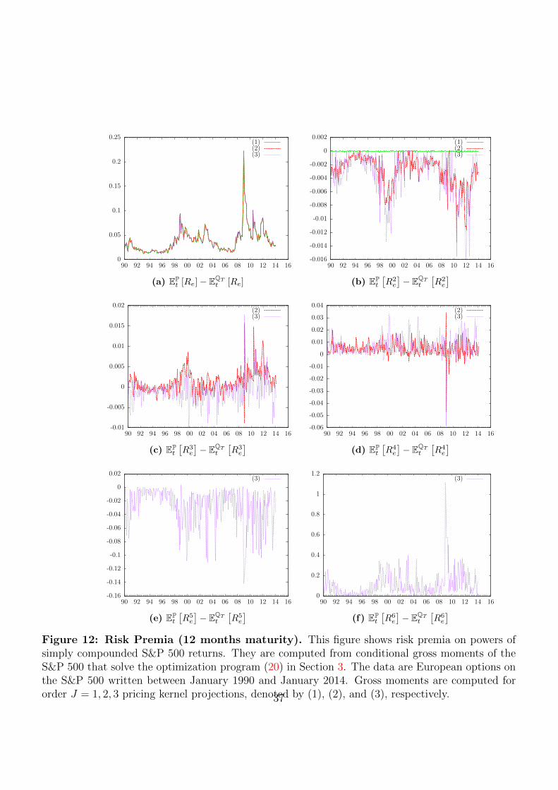
[R6

e

]− EQT

t

[R6

e

]Figure 9: Risk Premia (1 month maturity). This figure shows risk premia on powers of simplycompounded S&P 500 returns. They are computed from conditional gross moments of the S&P500 that solve the optimization program (20) in Section 3. The data are European options on theS&P 500 written between January 1990 and January 2014. Gross moments are computed for orderJ = 1, 2, 3 pricing kernel projections, denoted by (1), (2), and (3), respectively.34

0

0.02

0.04

0.06

0.08

0.1

0.12

0.14

0.16

90 92 94 96 98 00 02 04 06 08 10 12 14 16

(1)(2)(3)

(a) EPt [Re]− EQT

t [Re]

-0.012

-0.01

-0.008

-0.006

-0.004

-0.002

0

0.002

90 92 94 96 98 00 02 04 06 08 10 12 14 16

(1)(2)(3)

(b) EPt

[R2

e

]− EQT

t

[R2

e

]

-0.008

-0.006

-0.004

-0.002

0

0.002

0.004

0.006

0.008

0.01

90 92 94 96 98 00 02 04 06 08 10 12 14 16

(2)(3)

(c) EPt

[R3

e

]− EQT

t

[R3

e

] -0.02

-0.015

-0.01

-0.005

0

0.005

0.01

0.015

0.02

0.025

90 92 94 96 98 00 02 04 06 08 10 12 14 16

(2)(3)

(d) EPt

[R4

e

]− EQT

t

[R4

e

]

-0.1

-0.09

-0.08

-0.07

-0.06

-0.05

-0.04

-0.03

-0.02

-0.01

0

0.01

90 92 94 96 98 00 02 04 06 08 10 12 14 16

(3)

(e) EPt

[R5

e

]− EQT

t

[R5

e

] -0.05

0

0.05

0.1

0.15

0.2

0.25

0.3

0.35

0.4

0.45

0.5

90 92 94 96 98 00 02 04 06 08 10 12 14 16

(3)

(f) EPt

[R6

e

]− EQT

t

[R6

e

]Figure 10: Risk Premia (3 months maturity). This figure shows risk premia on powers ofsimply compounded S&P 500 returns. They are computed from conditional gross moments of theS&P 500 that solve the optimization program (20) in Section 3. The data are European options onthe S&P 500 written between January 1990 and January 2014. Gross moments are computed fororder J = 1, 2, 3 pricing kernel projections, denoted by (1), (2), and (3), respectively.35

0

0.02

0.04

0.06

0.08

0.1

0.12

0.14

0.16

90 92 94 96 98 00 02 04 06 08 10 12 14 16

(1)(2)(3)

(a) EPt [Re]− EQT

t [Re]

-0.012

-0.01

-0.008

-0.006

-0.004

-0.002

0

0.002

90 92 94 96 98 00 02 04 06 08 10 12 14 16

(1)(2)(3)

(b) EPt

[R2

e

]− EQT

t

[R2

e

]

-0.006

-0.004

-0.002

0

0.002

0.004

0.006

0.008

0.01

0.012

0.014

90 92 94 96 98 00 02 04 06 08 10 12 14 16

(2)(3)

(c) EPt

[R3

e

]− EQT

t

[R3

e

] -0.02

-0.015

-0.01

-0.005

0

0.005

0.01

0.015

0.02

0.025

90 92 94 96 98 00 02 04 06 08 10 12 14 16

(2)(3)

(d) EPt

[R4

e

]− EQT

t

[R4

e

]

-0.14

-0.12

-0.1

-0.08

-0.06

-0.04

-0.02

0

0.02

90 92 94 96 98 00 02 04 06 08 10 12 14 16

(3)

(e) EPt

[R5

e

]− EQT

t

[R5

e

] -0.1

0

0.1

0.2

0.3

0.4

0.5

0.6

0.7

0.8

90 92 94 96 98 00 02 04 06 08 10 12 14 16

(3)

(f) EPt

[R6

e

]− EQT

t

[R6

e


0

0.05

0.1

0.15

0.2

0.25

90 92 94 96 98 00 02 04 06 08 10 12 14 16

(1)(2)(3)

(a) EPt [Re]− EQT

t [Re]

-0.016

-0.014

-0.012

-0.01

-0.008

-0.006

-0.004

-0.002

0

0.002

90 92 94 96 98 00 02 04 06 08 10 12 14 16

(1)(2)(3)

(b) EPt

[R2

e

]− EQT

t

[R2

e

]

-0.01

-0.005

0

0.005

0.01

0.015

0.02

90 92 94 96 98 00 02 04 06 08 10 12 14 16

(2)(3)

(c) EPt

[R3

e

]− EQT

t

[R3

e

] -0.06

-0.05

-0.04

-0.03

-0.02

-0.01

0

0.01

0.02

0.03

0.04

90 92 94 96 98 00 02 04 06 08 10 12 14 16

(2)(3)

(d) EPt

[R4

e

]− EQT

t

[R4

e

]

-0.16

-0.14

-0.12

-0.1

-0.08

-0.06

-0.04

-0.02

0

0.02

90 92 94 96 98 00 02 04 06 08 10 12 14 16

(3)

(e) EPt

[R5

e

]− EQT

t

[R5

e

] 0

0.2

0.4

0.6

0.8

1

1.2

90 92 94 96 98 00 02 04 06 08 10 12 14 16

(3)

(f) EPt

[R6

e

]− EQT

t

[R6

e


1

1.01

1.02

1.03

1.04

1.05

1.06

90 92 94 96 98 00 02 04 06 08 10 12 14 16

(1)(2)(3)

(a) 1 month

1

1.02

1.04

1.06

1.08

1.1

1.12

1.14

1.16

90 92 94 96 98 00 02 04 06 08 10 12 14 16

(1)(2)(3)

(b) 3 months

1

1.05

1.1

1.15

1.2

1.25

90 92 94 96 98 00 02 04 06 08 10 12 14 16

(1)(2)(3)

(c) 6 months

1

1.05

1.1

1.15

1.2

1.25

1.3

1.35

90 92 94 96 98 00 02 04 06 08 10 12 14 16

(1)(2)(3)

(d) 12 months

Figure 13: Conditional Second Moment of Pricing Kernel. The panels show the time-varying conditional second moment of the pricing kernel projection (15) on simply compoundedS&P 500 returns for orders j = 1, 2, 3. The moments are solutions of the optimization program (20)in Section 3. The data are European options on the S&P 500 written between January 1990 andJanuary 2014.

38

0.96

0.98

1

1.02

1.04

1.06

1.08

90 92 94 96 98 00 02 04 06 08 10 12 14 16

(1)(2)(3)

(a) a0

-3

-2

-1

0

1

2

3

4

90 92 94 96 98 00 02 04 06 08 10 12 14 16

(1)(2)(3)

(b) a1

-25

-20

-15

-10

-5

0

5

10

15

20

25

30

90 92 94 96 98 00 02 04 06 08 10 12 14 16

(2)(3)

(c) a2

-25

-20

-15

-10

-5

0

5

10

15

90 92 94 96 98 00 02 04 06 08 10 12 14 16

(3)

(d) a3

Figure 14: Coefficients of Pricing Kernel Projection (1 month maturity). The panelsshow the coefficients of the projection (23) on simply compounded S&P 500 returns for ordersj = 1, 2, 3. The moments are solutions of the optimization program (20) in Section 3. The data areEuropean options on the S&P 500 written between January 1990 and January 2014.

39

0.95

1

1.05

1.1

1.15

1.2

1.25

90 92 94 96 98 00 02 04 06 08 10 12 14 16

(1)(2)(3)

(a) a0

-1.8

-1.7

-1.6

-1.5

-1.4

-1.3

-1.2

-1.1

-1

-0.9

-0.8

-0.7

90 92 94 96 98 00 02 04 06 08 10 12 14 16

(1)(2)(3)

(b) a1

-12

-10

-8

-6

-4

-2

0

2

4

6

90 92 94 96 98 00 02 04 06 08 10 12 14 16

(2)(3)

(c) a2

-4

-3

-2

-1

0

1

2

3

4

90 92 94 96 98 00 02 04 06 08 10 12 14 16

(3)

(d) a3

Figure 15: Coefficients of Pricing Kernel Projection (3 months maturity). The panelsshow the coefficients of the projection (23) on simply compounded S&P 500 returns for ordersj = 1, 2, 3. The moments are solutions of the optimization program (20) in Section 3. The data areEuropean options on the S&P 500 written between January 1990 and January 2014.

40

0.9

0.95

1

1.05

1.1

1.15

1.2

1.25

1.3

90 92 94 96 98 00 02 04 06 08 10 12 14 16

(1)(2)(3)

(a) a0

-1.9

-1.8

-1.7

-1.6

-1.5

-1.4

-1.3

-1.2

-1.1

-1

-0.9

-0.8

90 92 94 96 98 00 02 04 06 08 10 12 14 16

(1)(2)(3)

(b) a1

-8

-6

-4

-2

0

2

4

90 92 94 96 98 00 02 04 06 08 10 12 14 16

(2)(3)

(c) a2

-12

-10

-8

-6

-4

-2

0

2

90 92 94 96 98 00 02 04 06 08 10 12 14 16

(3)

(d) a3

Figure 16: Coefficients of Pricing Kernel Projection (6 months maturity). The panelsshow the coefficients of the projection (23) on simply compounded S&P 500 returns for ordersj = 1, 2, 3. The moments are solutions of the optimization program (20) in Section 3. The data areEuropean options on the S&P 500 written between January 1990 and January 2014.

41

0.95

1

1.05

1.1

1.15

1.2

1.25

1.3

1.35

1.4

90 92 94 96 98 00 02 04 06 08 10 12 14 16

(1)(2)(3)

(a) a0

-1.9

-1.8

-1.7

-1.6

-1.5

-1.4

-1.3

-1.2

-1.1

-1

-0.9

90 92 94 96 98 00 02 04 06 08 10 12 14 16

(1)(2)(3)

(b) a1

-8

-6

-4

-2

0

2

4

90 92 94 96 98 00 02 04 06 08 10 12 14 16

(2)(3)

(c) a2

-3.5

-3

-2.5

-2

-1.5

-1

-0.5

0

0.5

1

1.5

2

90 92 94 96 98 00 02 04 06 08 10 12 14 16

(3)

(d) a3

Figure 17: Coefficients of Pricing Kernel Projection (12 months maturity). The panelsshow the coefficients of the projection (23) on simply compounded S&P 500 returns for ordersj = 1, 2, 3. The moments are solutions of the optimization program (20) in Section 3.

42

9092949698000204060810121416 -0.3-0.2

-0.10

0.10.2

0.3

0.70.80.9

11.11.21.31.4

M(Re)(1)

t Re

M(Re)(1)

0.70.80.911.11.21.31.4

(a) 1 month

9092949698000204060810121416 -0.5-0.4-0.3-0.2-0.1 0 0.10.20.30.40.5

0.40.60.8

11.21.41.61.8

2

M(Re)(1)

t Re

M(Re)(1)

0.40.60.811.21.41.61.82

(b) 12 months

Figure 18: Conditional Linear Kernel Projection (1 and 12 months). The figure shows thelinear projection (23) over time as a function of time and simply compounded returns for 1 monthmaturity (Panel (a)) and 12 months maturity (Panel (b)). The data are European options on theS&P 500 written between January 1990 and January 2014.

43

9092949698000204060810121416 -0.3-0.2

-0.10

0.10.2

0.3

0.60.70.80.9

11.11.21.31.41.5

M(Re)(2)

t Re

M(Re)(2)

0.60.70.80.911.11.21.31.41.5

(a) 1 month

9092949698000204060810121416 -0.5-0.4-0.3-0.2-0.1 0 0.10.20.30.40.5

0.20.40.60.8

11.21.41.61.8

2

M(Re)(2)

t Re

M(Re)(2)

0.20.40.60.811.21.41.61.82

(b) 12 months

Figure 19: Conditional Quadratic Kernel Projection (1 and 12 months). The figure showsthe quadratic projection (23) over time as a function of time and simply compounded returns for 1month maturity (Panel (a)) and 12 months maturity (Panel (b)). The data are European optionson the S&P 500 written between January 1990 and January 2014.

44

9092949698000204060810121416 -0.3-0.2

-0.10

0.10.2

0.3

0.40.60.8

11.21.41.61.8

22.2

M(Re)(3)

t Re

M(Re)(3)

0.40.60.811.21.41.61.822.2

(a) 1 month

9092949698000204060810121416 -0.5-0.4-0.3-0.2-0.1 0 0.10.20.30.40.5

00.20.40.60.8

11.21.41.61.8

2

M(Re)(3)

t Re

M(Re)(3)

00.20.40.60.811.21.41.61.82

(b) 12 months

Figure 20: Conditional Cubic Kernel Projection (1 and 12 months). The figure shows thecubic projection (23) over time as a function of time and simply compounded returns for 1 monthmaturity (Panel (a)) and 12 months maturity (Panel (b)). The data are European options on theS&P 500 written between January 1990 and January 2014.

45

0.7

0.8

0.9

1

1.1

1.2

1.3

-0.3 -0.2 -0.1 0 0.1 0.2 0.3

M(R

e)(1)

Re

5%mean95%

(a) 1 month

0.7

0.8

0.9

1

1.1

1.2

1.3

1.4

-0.3 -0.2 -0.1 0 0.1 0.2 0.3

M(R

e)(1)

Re

5%mean95%

(b) 3 months

0.6

0.7

0.8

0.9

1

1.1

1.2

1.3

1.4

-0.4 -0.3 -0.2 -0.1 0 0.1 0.2 0.3 0.4

M(R

e)(1)

Re

5%mean95%

(c) 6 month

0.5

0.6

0.7

0.8

0.9

1

1.1

1.2

1.3

1.4

1.5

1.6

-0.5 -0.4 -0.3 -0.2 -0.1 0 0.1 0.2 0.3 0.4 0.5

M(R

e)(1)

Re

5%mean95%

(d) 12 months

Figure 21: Unconditional Linear Kernel Projection. The panels show bootstrapped samplemeans over the conditional linear pricing kernel projections from Figure 18. The projection iscomputed from simply compounded returns on the S&P 500. The data are European options onthe S&P 500 written between January 1990 and January 2014.

46

0.6

0.7

0.8

0.9

1

1.1

1.2

1.3

-0.3 -0.2 -0.1 0 0.1 0.2 0.3

M(R

e)(2)

Re

5%mean95%

(a) 1 month

0.6

0.7

0.8

0.9

1

1.1

1.2

1.3

1.4

-0.3 -0.2 -0.1 0 0.1 0.2 0.3

M(R

e)(2)

Re

5%mean95%

(b) 3 months

0.5

0.6

0.7

0.8

0.9

1

1.1

1.2

1.3

1.4

1.5

-0.4 -0.3 -0.2 -0.1 0 0.1 0.2 0.3 0.4

M(R

e)(2)

Re

5%mean95%

(c) 6 month

0.4

0.6

0.8

1

1.2

1.4

1.6

-0.5 -0.4 -0.3 -0.2 -0.1 0 0.1 0.2 0.3 0.4 0.5

M(R

e)(2)

Re

5%mean95%

(d) 12 months

Figure 22: Unconditional Quadratic Kernel Projection. The panels show bootstrappedsample means over the conditional quadratic pricing kernel projections from Figure 19. The projec-tion is computed from simply compounded returns on the S&P 500. The data are European optionson the S&P 500 written between January 1990 and January 2014.

47

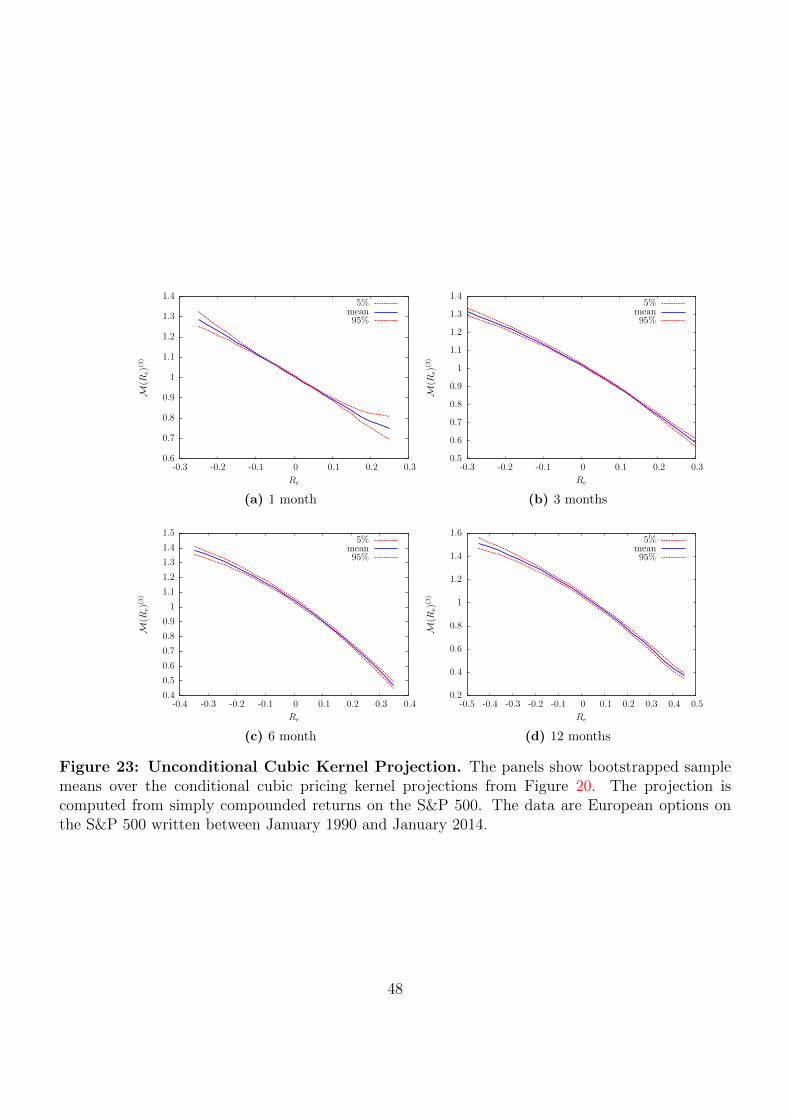
0.6

0.7

0.8

0.9

1

1.1

1.2

1.3

1.4

-0.3 -0.2 -0.1 0 0.1 0.2 0.3

M(R

e)(3)

Re

5%mean95%

(a) 1 month

0.5

0.6

0.7

0.8

0.9

1

1.1

1.2

1.3

1.4

-0.3 -0.2 -0.1 0 0.1 0.2 0.3

M(R

e)(3)

Re

5%mean95%

(b) 3 months

0.4

0.5

0.6

0.7

0.8

0.9

1

1.1

1.2

1.3

1.4

1.5

-0.4 -0.3 -0.2 -0.1 0 0.1 0.2 0.3 0.4

M(R

e)(3)

Re

5%mean95%

(c) 6 month

0.2

0.4

0.6

0.8

1

1.2

1.4

1.6

-0.5 -0.4 -0.3 -0.2 -0.1 0 0.1 0.2 0.3 0.4 0.5

M(R

e)(3)

Re

5%mean95%

(d) 12 months

Figure 23: Unconditional Cubic Kernel Projection. The panels show bootstrapped samplemeans over the conditional cubic pricing kernel projections from Figure 20. The projection iscomputed from simply compounded returns on the S&P 500. The data are European options onthe S&P 500 written between January 1990 and January 2014.

48

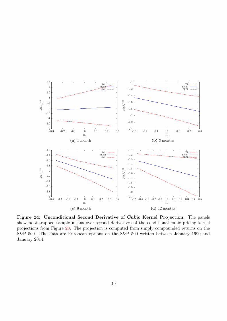
-2

-1.5

-1

-0.5

0

0.5

1

1.5

2

2.5

-0.3 -0.2 -0.1 0 0.1 0.2 0.3

M(R

e)(3)

Re

5%mean95%

(a) 1 month

-2.4

-2.2

-2

-1.8

-1.6

-1.4

-1.2

-1

-0.3 -0.2 -0.1 0 0.1 0.2 0.3

M(R

e)(3)

Re

5%mean95%

(b) 3 months

-3

-2.8

-2.6

-2.4

-2.2

-2

-1.8

-1.6

-1.4

-1.2

-0.4 -0.3 -0.2 -0.1 0 0.1 0.2 0.3 0.4

M(R

e)(3)

Re

5%mean95%

(c) 6 month

-2.1

-2

-1.9

-1.8

-1.7

-1.6

-1.5

-1.4

-1.3

-1.2

-1.1

-0.5 -0.4 -0.3 -0.2 -0.1 0 0.1 0.2 0.3 0.4 0.5

M(R

e)(3)

Re

5%mean95%

(d) 12 months

Figure 24: Unconditional Second Derivative of Cubic Kernel Projection. The panelsshow bootstrapped sample means over second derivatives of the conditional cubic pricing kernelprojections from Figure 20. The projection is computed from simply compounded returns on theS&P 500. The data are European options on the S&P 500 written between January 1990 andJanuary 2014.

49

1 m 1 2 3 4 5 6J=1 0.019 -0.33J=2 0.019 -0.24 -0.42 -97.50J=3 0.019 -0.27 -0.86 -72.65 -13517.75 -3948843.883 m 1 2 3 4 5 6J=1 0.013 -0.42J=2 0.013 -0.32 -0.12 -4.41J=3 0.013 -0.33 -0.24 -5.56 -246.67 -21622.466 m 1 2 3 4 5 6J=1 0.029 -0.082J=2 0.029 -0.019 -0.081 -2.69J=3 0.029 -0.011 -0.17 -2.99 -141.39 -13257.7412 m 1 2 3 4 5 6J=1 0.0034 0.076J=2 0.0033 0.12 0.0067 -1.05J=3 0.0041 0.13 -0.02 -1.88 -105.28 -9829.60

Table 1: Predictions. The table shows out-of-sample R2 from predictive regressions using theconditional moments from the solution of the minimization program (20). They are computed fromthe definition

R2 := 1−∑n

i=1(yi − yi)2∑ni=1(yi − yi)2

(C.17)

taken from Campbell and Thompson (2008), where yi denotes our prediction and yi denotes thesample mean on the basis of the data up to time i− 1. The data are European options written onthe S&P 500 from January 1990 to January 2014.

Order 1 2 31 month -0.13 -0.12 -0.0673 months -0.22 -0.20 -0.0646 months -0.31 -0.31 -0.2912 months -0.38 -0.38 -0.38

Table 2: Realized Sharpe Ratios. The table shows empirical Sharpe ratios from trading theprojection (23) for orders J = 1, 2, 3. The data are European options written on the S&P 500 fromJanuary 1990 to January 2014.

50

References

Acciaio, B., Beiglbock, M., Penkner, F., and Schachermayer, W. (2013). Amodel-free version of the fundamental theorem of asset pricing and thesuper-replication theorem. Mathematical Finance, pages n/a–n/a.

Aıt-Sahalia, Y. and Duarte, J. (2003). Nonparametric option pricing undershape restrictions. Journal of Econometrics, 16:9–47.

Aıt-Sahalia, Y. and Hansen, L. P., editors (2009). Handbook of FinancialEconometrics. Elsevier.

Aıt-Sahalia, Y. and Lo, A. W. (1998). Nonparametric estimation of state-price densities implicit in financial asset prices. Journal of Finance,53(2):499–547.

Aıt-Sahalia, Y. and Lo, A. W. (2000). Nonparametric risk management andimplied risk aversion. Journal of Econometrics, 94:9–51.

Almeida, C. and Garcia, R. (2015). Economic implications of nonlinear pric-ing kernels. Working paper, Getulio Vargas Foundation and EDHEC Busi-ness School.

Alvarez, F. and Jermann, U. (2005). Using asset prices to measure thepersistence of the marginal utility of wealth. Econometrica, 73:1977–2016.

Bakshi, G., Madan, D., and Panayotov, G. (2010). Returns of claims on theupside and the viability of U-shaped pricing kernels. Journal of FinancialEconomics, 97:130–154.

Beare, B. K. and Schmidt, L. D. W. (2014). An empirical test of pricingkernel monotonicity. Journal of Applied Econometrics, pages n/a–n/a.

Birke, M. and Pilz, K. (2009). Nonparametric option pricing with no-arbitrage constraints. Journal of Financial Econometrics, 7:53–76.

Borovicka, J., Hansen, L. P., and Scheinkman, J. (2014). Misspecified recov-ery. Working paper, New York University, University of Chicago, PrincetonUniversity and NBER.

Breeden, D. T. and Litzenberger, R. H. (1978). Prices of state-contingentclaims implicit in option prices. Journal of Business, 51:621–651.

Campbell, J. Y. and Thompson, S. B. (2008). Predicting excess stock returnsout of sample: Can anything beat the historical average? Review ofFinancial Studies, 21:1509–1531.

51

Carr, P. and Madan, D. (2001). Towards a theory of volatility trading. InJouini, E., Cvitanic, J., and Musiela, M., editors, Option Pricing, InterestRates and Risk Management, Handbooks in Mathematical Finance, pages458–476. Cambridge University Press.

Carr, P. and Wu, L. (2009). Variance risk premiums. Review of FinancialStudies, 22:1311–1341.

Carr, P. and Yu, J. (2012). Risk, return, and ross recovery. Journal ofDerivatives, 20:38–59.

CBOE (2009). The CBOE volatility index - VIX. CBOE.

Chabi-Yo, F., Garcia, R., and Renault, E. (2008). State dependence canexplain the risk aversion puzzle. Review of Financial Studies, 21:973–1011.

Chapman, D. A. (1997). Approximating the asset pricing kernel. Journal ofFinance, 52:1383–1410.

Chernozhukov, V. and Hong, H. (2003). An mcmc approach to classicalestimation. Journal of Econometrics, 115:293–346.

Cochrane, J. and Saa-Requejo, J. (2000). Beyond arbitrage: Good-deal as-set pricing bounds in incomplete markets. Journal of Political Economy,108:79–119.

Cont, R., editor (2010). Encyclopedia of Quantitative Finance. Wiley.

Curto, R. and Fialko, L. (1991). Recursiveness, positivity, and truncatedmoment problems. Houston Journal of Mathematics, 17:603–635.

Eraker, B. (2004). Do stock prices and volatility jump? Reconciling evidencefrom spot and option prices. Journal of Finance, 59(3):1367–1404.

Filipovic, D., Mayerhofer, E., and Schneider, P. (2013). Transition densityapproximations for multivariate affine jump diffusion processes. Journalof Econometrics, 176:93–111.

Garcia, R., Ghysels, E., and Renault, E. (2009). The Econometrics of OptionPricing. In Aıt-Sahalia and Hansen (2009).

Gosh, A., Julliard, C., and Taylor, A. (2013). What is the consumptioncapm missing? an information-theoretic framework for the analysis of assetpricing models. Working paper, Tepper School of Business, London Schoolof Economics and Political Science, and Manchester Business School.

52

Hansen, L. P. and Jagannathan, R. (1997). Assessing specification errors instochastic discount factor models. Journal of Finance, 52:557–590.

Hansen, L. P. and Renault, E. (2010). Pricing Kernels. In Cont (2010).

Hansen, L. P. and Scheinkman, J. (2009). Long-term risk: An operatorapproach. Econometrica, 77:177–234.

Heston, S. (1993). A closed-form solution for options with stochastic volatil-ity with applications to bond and currency options. Review of FinancialStudies, 6:327–343.

Jackwerth, J. (2000). Recovering risk aversion from option prices and realizedreturns. Review of Financial Studies, 13:433–451.

Jones, C. (2003). The dynamics of stochastic volatility: evidence from un-derlying and options markets. Journal of Econometrics, 116:181–224.

Julliard, C. and Ghosh, A. (2012). Can rare events explain the equity pre-mium puzzle? Review of Financial Studies, 25:3037–3076.

Kozhan, R., Neuberger, A., and Schneider, P. (2013). The skew risk premiumin the equity index market. Review of Financial Studies, 26:2174–2203.

Martin, I. (2013). Simple variance swaps. Working paper, Stanford Univer-sity.

Martin, I. (2015). What is the expected return on the market? Workingpaper, London School of Economics and Political Science.

Neal, R. (2015). Fast exact summation using small and large superaccumu-lators. Technical report, University of Toronto.

Ross, S. (2015). The recovery theorem. Journal of Finance, 70:615–648.

Schmidt, K. (2003). On the covariance of monotone functions of a randomvariable. Working paper, Technische Universitat Dresden.

Schneider, P. (2015). Generalized risk premia. Journal of Financial Eco-nomics, 116:487 – 504.

Schneider, P. and Trojani, F. (2014). Fear trading. Working paper, Universityof Lugano and SFI.

Schneider, P. and Trojani, F. (2015). Divergence and the price of uncertainty.Working paper, University of Lugano and SFI.

53

Song, Z. and Xiu, D. (2014). A tale of two option markets: Pricing kernelsand volatility risk. Board of Governors of the Federal Reserve System(U.S.).

Cerny, A. (2003). Generalised sharpe ratios and asset pricing in incompletemarkets. European Finance Review, 7:191–233.

54

(almost) model-free recovery - brown university · (almost) model-free recovery paul schneideryand...

Documents