ambiguity aversion and stock market participation

1

Ambiguity Aversion and Stock Market Participation:

Evidence from Fund Flows

Constantinos Antoniou, Richard D. F. Harris, Ruogu Zhang*

June 2013

Abstract

Stock market participation is very low, with approximately two thirds of all

U.S. households not owning any public equity. This is a puzzle in the

context of the basic Expected Utility model. One explanation put forward in

the literature is that stock market participation is low because, in addition to

risk, stocks also entail ambiguity and investors are ambiguity averse. We

empirically test this hypothesis, measuring stock market participation using

equity fund flows and ambiguity with dispersion in analyst forecasts about

aggregate market returns. In a multivariate framework our results show that

increases in ambiguity are significantly and negatively related to equity fund

flows, and thus support the notion that limited market participation is related

to ambiguity aversion.

Keywords: Stock market participation; ambiguity aversion; fund flows.

*Xfi Centre for Finance and Investment, University of Exeter Business School, Streatham Court, Rennes Drive,

Exeter, EX4 4ST, U.K. E-mails: [email protected] (Antoniou), [email protected]

(Harris),[email protected] (Zhang). We thank Emilios Galariotis, Giakomo Nocera, Rajesh Tharyan,

Grzegorz Trojanowski, Christophe Villa and seminar participants at Exeter University and Audencia Nantes for

useful comments and suggestions. We also thank the Investment Company Institute (ICI) for providing us with

the data on fund flows, Mark Kamstra for sharing the data on capital gains.

.

2

Ambiguity Aversion and Stock Market Participation:

Evidence from Fund Flows

June 2013

Abstract

Stock market participation is very low, with approximately two thirds of all

U.S. households not owning any public equity. This is a puzzle in the

context of the basic Expected Utility model. One explanation put forward in

the literature is that stock market participation is low because, in addition to

risk, stocks also entail ambiguity and investors are ambiguity averse. We

empirically test this hypothesis, measuring stock market participation using

equity fund flows and ambiguity with dispersion in analyst forecasts about

aggregate market returns. In a multivariate framework our results show that

increases in ambiguity are significantly and negatively related to equity fund

flows, and thus support the notion that limited market participation is related

to ambiguity aversion.

Keywords: Stock market participation; ambiguity aversion; fund flows.

3

1. Introduction

During the last century the U.S. stock market has yielded an average annual return of approximately

eight percent over treasury bills (Mehra, 2003). Given this equity premium the canonical expected-

utility model (EU) predicts that agents with reasonable risk-aversion should be very willing to

participate in the stock market. However, stock market participation is very low. For the period 1982-

1995 the U.S. Consumer Expenditure Survey found that two thirds of all U.S. households do not

invest in stocks. Even at the eightieth percentile of wealth, almost 20% of households have no public

equity (Campbell, 2006). It is difficult to reconcile these results with the EU model, so this

phenomenon is widely known as the limited-participation puzzle.1

Various explanations have been put forward for the limited-participation puzzle. Williamson

(1994) and Allen and Gale (1994) suggest that liquidity needs and transaction costs deter stock market

participation. Hong, Kubik and Stein (2004) suggest that the fixed cost of entering the stock market

for the first time is too high, which also limits participation (see also Vissing-Jorgenson, 2002; Guiso,

Haliassos and Jappelli, 2003). Hsu (2012) argues that households with low human capital have less

need for diversification and therefore invest less in stocks. Haliassos and Bertatut (1996) suggest that

borrowing constraints and minimum investment requirements also reduce market participation.

However, these explanations cannot completely explain the non-participation puzzle, so some

researchers have resorted to ‘behavioural’ explanations.

One prominent behavioural explanation is that limited-participation is driven by ambiguity

aversion (Dow and Werlang, 1992; Mukerji and Tallon, 2001; Cao, Wang and Zhang, 2005; Easley

and O’Hara, 2009; Epstein and Schneider 2010; Werner, 2011; Takashi, 2011). The notion of

ambiguity was initially developed by Knight (1921) and Keynes (1921), and describes a situation

where the probabilities associated with future states of nature are unknown. Ellsberg (1961) was the

first to conjecture that people are particularly averse to ambiguity, a result subsequently confirmed by

1 For a theoretical exposition of the puzzle see Haliassos and Bertaut (1995).

4

many studies in experimental economics and psychology.2 According to the ambiguity-based

explanation of the non-participation puzzle, stocks involve both risk and ambiguity. Owing to the fact

that the majority of people are averse to ambiguity, their propensity to invest in stocks is lower than

that implied by the EU model.3

In this paper we empirically examine whether ambiguity is negatively related to stock market

participation. The starting point for our analysis is the notion that for non-professional investors, the

principal avenue for broad-based stock market participation is through mutual funds. The Investment

Company Institute estimates that in 2011, households owned 89 percent of the mutual fund industry

(ICI Factbook, 2012). Therefore, flows in and out of mutual funds reflect the active reallocation

decisions of individual investors, and thus provide a direct measure of market participation.4

To test the hypothesis we require an empirical measure of ambiguity. To this end we rely on

the measure proposed in a recent study by Anderson, Ghysels and Juergens (2009), which reflects

dispersion in analysts’ forecasts using data from the Survey of Professional Forecasters (SPF), issued

by the Federal Reserve. The SPF contains forecasted quarterly data such as GDP growth and inflation

from different analysts, and following Anderson, Ghysels and Juergens (2009) we use the Gordon

Growth Model to derive a forecast for aggregate stock market return for each analyst. When

dispersion among analysts regarding the future performance of stock markets is high, ambiguity is

also likely to be high since experts have arrived at conflicting views regarding the fundamentals of the

economy. In these conditions it is possible that multiple distributions of expected returns are plausible,

2 A large literature, starting with Knight (1921) and Keynes (1921), and continuing through Ellsberg (1961) and

up to the present day (Ahn et al., 2011), shows that situations that involve ambiguity are treated differently from

those that involve risk. Hsu et al. (2005) and Levy et al. (2010) present evidence that ambiguous situations

produce a unique neurological fingerprint, suggesting that ambiguity aversion is rooted in the fundamentals of

human cognition. See Camerer and Weber (1992) and Keren and Gerritsen (1999) for reviews on the evidence

on ambiguity aversion. 3Hong, Kubik and Stein (2004) put forward an alternative behavioural explanation, based on social interaction.

Grinblatt, Keloharju and Linnainmaa (2011) show that cognitive ability also relates to market participation

decisions. 4 This measure does not capture total stock market participation decisions, however, as it omits households that

invest in stocks directly.

5

and that investors cannot confidently narrow down the set to the ‘correct’ one.5 We discuss this

measure in more detail in section 3.2 of the paper.

Using data on U.S. fund flows from the Investment Company Institute, we examine in a

multivariate framework whether ambiguity is related to capital flows into equity mutual funds,

controlling for other factors that have been shown to be important in explaining fund flows, including

risk. We use two empirical proxies for market participation: mutual fund flows, i.e. the net cash flow

into equity funds, and mutual fund exchanges, i.e. the switch of capital between funds of different

asset classes that are managed by the same investment house. Whilst the first measure captures stock

market participation in absolute terms, the second, proposed by Ben-Rephael, Kandel and Wohl

(2012), provides a stock-market participation metric that is relative to other asset classes.

In our models, we control for factors that have been previously documented to affect flows,

including past fund returns (Ippolito,1992; Sirri and Tufano, 1998), capital gains (Kamstra et al.,

2011), past flows (Ben-Rephael, Kandel, and Wohl, 2011), seasonal effects (Kamstra et al., 2011),

advertising expenses (Gallaher, Kaniel, and Starks, 2006), past market returns (Ben-Rephael, Kandel,

and Wohl, 2012) and savings (Kamstra et al., 2011). To ensure that the ambiguity measure we use is

not simply capturing risk, we include a measure of market risk in our regressions. Our results show

that controlling for other factors that affect changes in flows, increases in ambiguity are associated

with reductions in capital moving into equity mutual funds, using the categorization of Kamstra et al.

(2011). This finding confirms the prediction of the theoretical ambiguity literature, that market

participation is negatively related to ambiguity aversion.

Furthermore, when we dissect equity flows into different categories, we find that the effect of

ambiguity is concentrated in funds classed as ‘aggressive growth’ and ‘growth’, which are the those

that invest in more ambiguous firms, and hence more likely to be eschewed by investors in periods of

high ambiguity. We also analyze flows in and out of non-equity mutual funds and find that ambiguity

is positively related to mutual fund exchanges into money market funds. Since money market funds

5 Drechsler (2012) uses a very similar dispersion-based measure of ambiguity, calculated from the SPF data.

6

invest in safer, short-term high-grade securities, a plausible explanation for this result is that investors

are seeking a safer and more liquid asset class when faced with higher ambiguity in expected equity

returns.

Our study contributes to the literature that analyzes stock market participation by empirically

examining the prediction made by several theoretical studies, that ambiguity deters investors from

entering the stock market (Dow and Werlang, 1992; Mukerji and Tallon, 2001; Easley and O’Hara,

2009; Epstein and Schneider, 2010; Werner, 2011; Takashi, 2011). Our evidence supports these

theories, highlighting that limited stock market participation is negatively related to ambiguity.

Our study also contributes to the literature that analyzes the determinants of fund flows. Jain

and Wu (2000) and Kacperczyk and Seru (2007) show that fund flows are related to funds’

advertising expenses and the ability of the fund manager, respectively. Ivkovich and Weisbenner

(2009) show that flows are affected by past fund performance, expense ratios and loads. Cooper,

Gulen and Rau (2005) show that flows are affected by catering effects via name changes, and Kamstra,

Kramer, Levi and Wermers (2011) show that flows are affected by seasonal variations in risk aversion.

Our study shows that flows are negatively related to ambiguity about future stock market returns.

The literature on ambiguity in financial markets has thus far mainly concentrated on the

theoretical tools of analysis (for reviews of this literature, see Epstein and Schneider, 2010, and

Mukerji and Tallon, 2003). It is important, however, to empirically test the predictions of these

theories, and thus far the literature has relied mainly on the experimental tools of analysis (Camerer

and Kunreuther, 1989; Sarin and Weber, 1993; Ahn et al., 2009; Bossaerts et al., 2010). More recently,

however, several studies bring the predictions of the theoretical literature to financial data. Anderson,

Ghysels and Juergens (2009) show that market returns exhibit a significant ambiguity premium,

which is stronger than the risk premium. Antoniou, Galariotis and Read (2012) examine the response

of investors to ambiguous information, as discussed theoretically in Epstein and Schneider (2008),

and Kelsey, Kozhan and Pang (2010) analyze the link between violations of weak-form market

efficiency and ambiguity (see also the theoretical discussion by Caskey, 2009). Our study shows that

7

ambiguity affects market participation. These studies highlight that ambiguity has important effects on

financial markets that cannot be captured by the EU model.

The next section reviews the relevant literature in more detail and develops the hypothesis.

The third section describes the data, the fourth presents and discusses the empirical analysis and the

final section concludes the paper.

2. Ambiguity and market participation

In this section we use a simple model to develop our hypothesis. We begin with the basic EU model

and then extend it to show how ambiguity can affect market participation. Our exposition follows

Banerjee and Green (2012).

The economy has a representative agent and two assets: a risk free asset and a risky asset. The

gross risk-free rate is normalized to The risky asset pays a stream of i.i.d. dividends

. The aggregate supply of the risky asset is constant and equal to Z. The price of the risky

asset at time t is and the dollar return is denoted:

(1)

The representative investor has standard mean-variance preferences over next period’s wealth and

submits a limit order for the risky asset such that:

][var2

][maxarg 11 ttttttx

t xQRWa

xQRWx (2)

where and denote the conditional expectation and conditional variance of next period’s

wealth, respectively, given date t information, is the wealth invested in the risk free asset, and α is

the coefficient of risk aversion. The optimal demand for the risky asset is:

(3)

8

where reflects the investor’s stock market participation at time t. increases in expected returns

and decreases in variance (proportionately to risk aversion).

In this model it is implicitly assumed that the decision maker is able to uniquely estimate a

conditional probability distribution for the asset payoffs, and is thus making a decision in conditions

of risk. Ambiguity, however, is a situation in which the decision maker does not have enough

information to arrive at a single probability distribution and faces a situation where multiple

likelihoods can plausibly arise.

To illustrate the concept of ambiguity and its impact on choices we provide the following

example, adapted from Ellsberg’s (1961) seminal work. After we discuss this example we extend the

above model to illustrate the effect of ambiguity on stock market participation.

Assume we have two urns with 100 balls in each. The first urn contains 50 red and 50 black

balls, whereas the second contains red and black balls in unknown proportions. The first urn is risky

because the probability distribution that describes its contents is known with certainty. However, the

second is ambiguous since many different distributions are possible (i.e., 0 red and 100 black, 1 red

and 99 black, etc). Note that there is no way for the agent to resolve this ambiguity and determine

with certainty the distribution that describes the contents of the second urn. Suppose that a decision

maker is paid an amount c>0 if he bets on an event that actually occurs (i.e., a draw of a ball from

either urn). This decision maker is presented with the following options:

Bet A: bet on red from the first urn Bet B: bet on red from second urn

After a choice is made between bets A and B the decision maker is faced with two more choices:

Bet C: bet on black from the first urn Bet D: bet on black from second urn

Experimental evidence shows that the majority of people prefer bet A over bet B (A>B),

which suggests a belief that pr(black ball from second urn) >pr(black from first urn). However, when

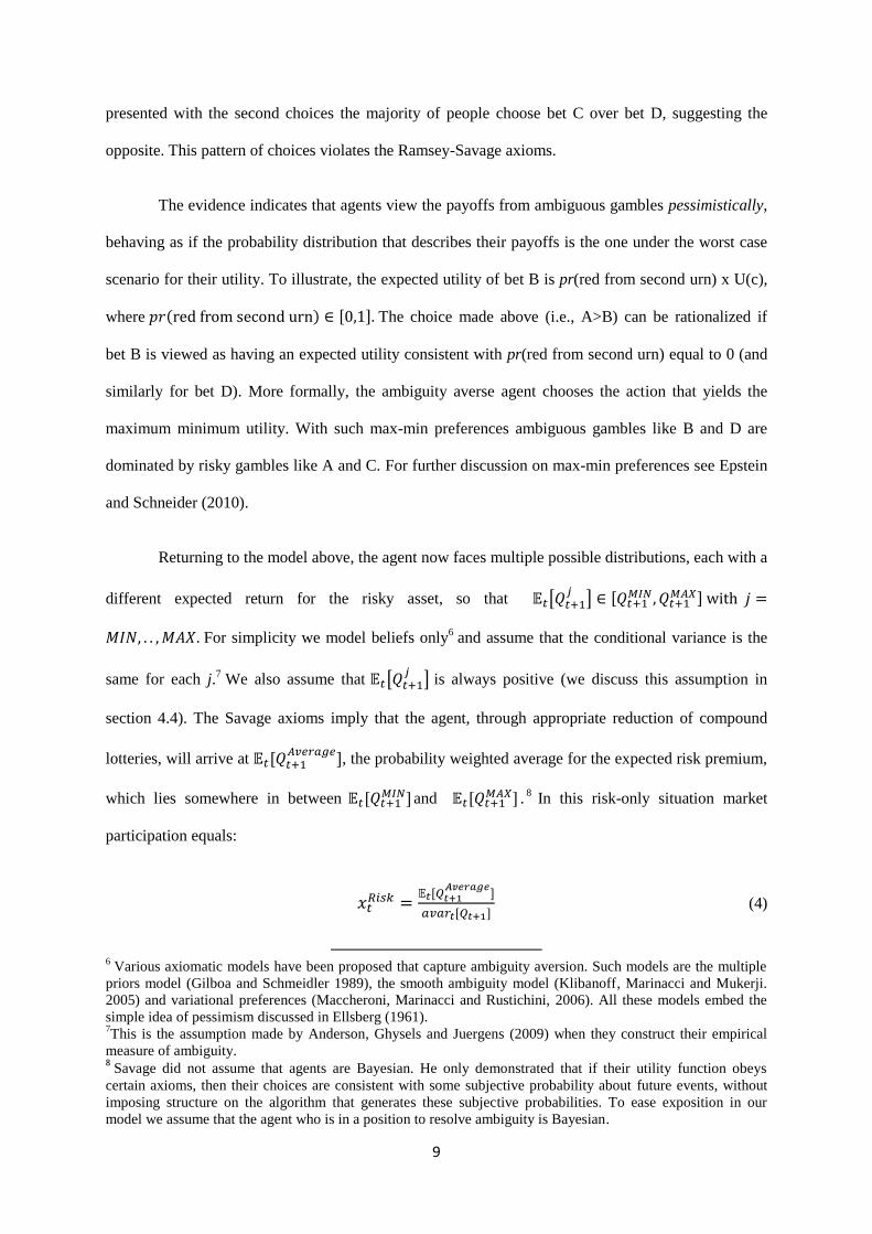
9

presented with the second choices the majority of people choose bet C over bet D, suggesting the

opposite. This pattern of choices violates the Ramsey-Savage axioms.

The evidence indicates that agents view the payoffs from ambiguous gambles pessimistically,

behaving as if the probability distribution that describes their payoffs is the one under the worst case

scenario for their utility. To illustrate, the expected utility of bet B is pr(red from second urn) x U(c),

where The choice made above (i.e., A>B) can be rationalized if

bet B is viewed as having an expected utility consistent with pr(red from second urn) equal to 0 (and

similarly for bet D). More formally, the ambiguity averse agent chooses the action that yields the

maximum minimum utility. With such max-min preferences ambiguous gambles like B and D are

dominated by risky gambles like A and C. For further discussion on max-min preferences see Epstein

and Schneider (2010).

Returning to the model above, the agent now faces multiple possible distributions, each with a

different expected return for the risky asset, so that

For simplicity we model beliefs only6 and assume that the conditional variance is the

same for each j.7 We also assume that

is always positive (we discuss this assumption in

section 4.4). The Savage axioms imply that the agent, through appropriate reduction of compound

lotteries, will arrive at

, the probability weighted average for the expected risk premium,

which lies somewhere in between and

.8 In this risk-only situation market

participation equals:

(4)

6 Various axiomatic models have been proposed that capture ambiguity aversion. Such models are the multiple

priors model (Gilboa and Schmeidler 1989), the smooth ambiguity model (Klibanoff, Marinacci and Mukerji.

2005) and variational preferences (Maccheroni, Marinacci and Rustichini, 2006). All these models embed the

simple idea of pessimism discussed in Ellsberg (1961). 7This is the assumption made by Anderson, Ghysels and Juergens (2009) when they construct their empirical

measure of ambiguity. 8 Savage did not assume that agents are Bayesian. He only demonstrated that if their utility function obeys

certain axioms, then their choices are consistent with some subjective probability about future events, without

imposing structure on the algorithm that generates these subjective probabilities. To ease exposition in our

model we assume that the agent who is in a position to resolve ambiguity is Bayesian.

10

However, if the agent cannot assign probabilities to the possible distributions (as explained in the

above thought experiment) he faces ambiguity. Being ambiguity averse he makes decisions

pessimistically so stock market participation will be determined according to the worst case risk

premium:

(5)

In conditions of ambiguity market participation is therefore lower, i.e.,

< . The level

of ambiguity faced by the agent is captured by the distance

If this distance increases

the agent faces more ambiguity and therefore becomes more pessimistic, as becomes lower.

Therefore we should observe a negative relationship between market participation and ambiguity

about expected stock returns.

3. Data

3.1 Mutual Fund Flows and Exchanges

Our main source of fund data is the Investment Company Institute (ICI), which provides

detailed information about the monthly flows to thirty mutual funds investment categories. Our

sample covers the period January 1984 to December 2010. For each fund category, ICI reports

monthly data on sales, redemptions, exchanges, reinvested distributions and total net assets. We

divide the thirty ICI investment objective categories into five groups by asset class using the

categorization proposed by Kamstra et al. (2011), namely equity, hybrid, corporate fixed income,

government fixed income and money market. Our main focus is the equity asset class, which

comprises funds classified as ‘aggressive growth’, ‘growth’, ‘sector’, ‘growth and income’, and

‘income equity’. Moreover, since the ambiguity measure that we construct is for the U.S. stock market,

we omit the equity investment objective categories that represent investments outside of the U.S., i.e.

‘global equity’, ‘international equity’, ‘regional equity’ and ‘emerging markets’. When we analyse

11

flows into non-equity funds we eliminate ‘global bond – general’, ‘global bond – short term’ and

‘other world bond’ fund categories. In Table 1 we report the classification of funds by investment

objective category.

[Table 1 here]

We compute the net cash inflow into asset class i in month t as:

(6)

Similarly, following Ben-Rephael, Kandel, and Wohl (2012), we compute the net exchange into asset

class i in month t as:

(7)

Figure 1 plots the net flows and exchanges for the equity group of funds. Net flows and

exchanges into equity were very much more volatile before 1993, with a large flow out of the equity

asset class following the October 1987 crash. Since 1994, net flows and net exchanges have been less

volatile, but also declining. Table 2 reports summary statistics for the net flows and exchanges for the

equity asset class. The average net flow is 0.51%, representing a substantial increase in total net assets

over the sample, while the average net exchange is close to zero. Net exchanges are negatively

skewed and strongly leptokurtic, while net flows have much lower skewness and kurtosis.

[Figure 1 here]

[Table 2 here]

3.2 Measuring ambiguity

Ellsberg’s (1961) definition of when ambiguity will arise remains the most perspicuous:

“Ambiguity is a subjective variable, but it should be possible to identify “objectively” some situations

likely to present high ambiguity, by noting situations where available information is scanty or

obviously unreliable or highly conflicting; or where expressed expectations of different individuals

12

differ widely;” Ellsberg (1961, p. 660). Ellsberg thus views ambiguity as negatively related to what

might be called the “richness” of the information that is available to compute the likelihood of

interest,9 and suggests two broad ways to empirically measure ambiguity: Either by quantifying the

richness of the information directly; or by inferring this richness indirectly using as an index the

disagreement between different users of the information set.

In our study we use the empirical measure of ambiguity proposed by Anderson, Ghysels and

Juergens (2009) (AGJ) which is based on the latter approach. This measure reflects disagreement

among experts regarding aggregate economic performance in the future. Experts analyze the available

information related to the future prospects of the economy, form a subjective probability distribution

and report the mean of this distribution as their forecast. High disagreement amongst these experts

implies an incomplete information set and, therefore, ambiguity. 10

The data to calculate this measure are taken from the Federal Reserve’s Survey of

Professional Forecasters (SPF), which reports the individual forecasts made by large financial

institutions of a number of U.S. economic and financial variables, for a range of forecast horizons

including the last quarter (the actual value of which may not have been published at the time the

forecast is made) and the following four quarters, as well as for annual and longer horizons. The

forecast data is available on a quarterly basis from 1968, and represents the views of between a

minimum of nine and a maximum of 74 participants. Following Anderson, Ghysels and Juergens

(2009), we use forecasts of aggregate output, the output deflator, and corporate profits after taxes.11

We first calculate an approximation of the forecast at time t of real aggregate corporate profit at time

t+1 for forecaster i as:

9 This view is common among decision theorists. Frisch and Baron (1988) proposed that “ambiguity is

uncertainty about probability, created by missing information that is relevant and could be known” (P. 1988).

Einhorn and Hogarth (1985) suggest that ambiguous situations arise when the available information is vague,

and does not allow one to confidently rule out alternative possibilities, while Gärdenfors and Sahlin (1982, 1983)

argue that feelings of ambiguity are produced when the relevance of the available information is low. 10

Antoniou et al. (2012) use the first approach suggested by Ellsberg (1961) and measure ambiguity in the cross

section of stocks by examining the extent to which analyst earnings forecast accuracy (the likelihood of interest

to decision makers that price earnings forecasts) can be predicted from factors such as analyst ability, forecast

timeliness, etc. 11

Output is defined as Gross National Product (GNP) before 1992Q1 and Gross Domestic Product (GDP)

thereafter. Similarly, the output deflator is the GNP deflator before 1992Q1 and the GDP deflator thereafter.

13

(8)

where is the real aggregate corporate profit level at time t, is the GDP deflator at time t, is the

nominal corporate profit level at time t. We then use the Gordon growth model to obtain the implied

forecast at time t of the market return at time t+1:

(9)

where is the aggregate market value in the U.S., obtained from the Flow of Funds Accounts of the

United States, published by the Federal Reserve, is the forecast at time t for forecaster i of the

gross real growth rate of corporate profits, which is calculated as the approximate forecast gross

growth rate from last quarter to three quarters ahead:

(10)

The forecast market return is computed every quarter from 1985Q1 to 2010Q4 (i.e., the

period for which we have available fund flow data), for all available forecasters. We then follow

Anderson et al (2009) and calculate a beta-weighted dispersion of the forecast market return each

quarter across individual forecasters. Define as the number of forecasts available in quarter t. In

each quarter t, we rank the forecasts from high to low, and assign a weight to the ith lowest forecast

of:

(11)

where the parameter determines the shape of the weight function: if =1 the forecasts are equally

weighted, while higher values of gives less weight to extreme forecasts. Our quarterly ambiguity

measure is given by:

(12)

14

In the empirical analysis, we use , which is the value used by Anderson, Ghysels and

Juergens (2009).

As the SPF data are available on a quarterly basis, and the fund flow data are available only

from 1985, we are left with a small sample of 102 data points, which does not allow a powerful test of

our hypothesis, especially given the large number of control variables that must be included in the

regressions. To circumvent this problem we convert the quarterly ambiguity series into a monthly

series using linear interpolation, and conduct the analysis using monthly data.12

To ensure, however,

that this procedure has no implications for our conclusions, in our robustness checks, discussed in

Section 4.3, we conduct the analysis using non-interpolated, quarterly data and obtain very similar

results.

In our models we consider the change rather than the level of ambiguity because our

hypothesis is that the degree of equity market participation, as measured by total net assets held by

mutual funds, is determined by the level of ambiguity, and so fund flows, which represent changes in

total net assets, are determined by changes in ambiguity. In equilibrium, for a given level of ambiguity,

fund flows will be zero, and so positive (negative) fund flows arise from decreases (increases) in

ambiguity. We estimate all our models using Newey and West (1987, 1994) heteroscedasticity and

autocorrelation consistent standard errors.

Panel A in Figure 2 plots the quarterly ambiguity measure and Panel B the changes in the

monthly interpolated series. Both measures produce spikes in the mid 1980s to mid 1990s and in the

2000s. Table 2 reports summary statistics for the constructed ambiguity series and for changes in the

monthly, interpolated series. Both series are moderately positively skewed and leptokurtic.

[Figure 2 here]

12

Specifically we calculate monthly ambiguity using quarter t and t+1 observations as follows:

, where i stands for the i

th month of quarter t.

15

3.4 Control Variables

Conditional Volatility

To ensure that the ambiguity measure is not just capturing risk, we include a measure of

conditional volatility in the model, following Andersen, Ghysels and Juergens (2009). In particular,

we compute the weighted variance of past squared excess market returns. The weight for ith lag is

given by:

(13)

where s is the minimum number of available trading days for the previous 12 months over the entire

sample, and the parameter determines the speed at which the weights decline as the lag length

increases. In the empirical analysis, we follow Anderson, Ghysels and Juergens (2009) and use

. The conditional variance is then given by:

*

1 =1 , , +1−1 =1 , (14)

where is the market excess return at ith lag, which is computed as the daily CRSP value-weighted

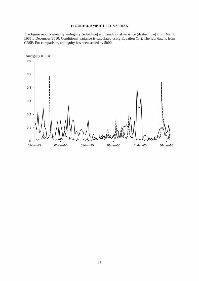
index (series VWRETD) return minus the daily return of the three month T-bill. Figure 3 plots the

monthly conditional variance together with the monthly ambiguity, for the period March 1985 to

December 2010. It is clear that the two series capture very different dimensions of the market, with

periods when ambiguity is high but conditional variance is low, and vice versa. Table 2 reports

summary statistics for conditional variance. As expected, the conditional variance is highly positively

skewed and leptokurtic. As with ambiguity, we use the changes in monthly conditional variance in our

regression, and Table 2 reports the descriptive statistics for this series. It can be seen that changes in

conditional variance are also positively skewed and leptokurtic.

[Figure 3 here]

16

Other Control Variables

There are a number of other factors that have been shown to be important in explaining

mutual fund flows, including past fund returns (Ippolito,1992; Sirri and Tufano, 1998), capital gains

(Kamstra et al., 2011), past flows (Ben-Rephael, Kandel and Wohl, 2011), seasonal effects (Kamstra

et al., 2011), advertising expenses (Gallaher, Kaniel and Starks, 2006), past market returns (Ben-

Rephael, Kandel and Wohl, 2012) and savings (Kamstra et al., 2011). We capture serial correlation in

fund flows by including lagged monthly net flows and net exchanges for the past one, three, six and

12 months. We include the personal savings rate from the Bureau of Economic Analysis (series

PSAVERT). The data on capital gains and advertising costs is from Kamstra et al. (2011).13

We

include the aggregate return of the equity fund group over the previous 12 months to capture return-

chasing behaviour and, following Ben-Rephael, Kandel and Wohl (2011) and Oh and Parwada (2007),

we also include the aggregate market return over the last three months. Since transaction costs and

liquidity needs have been proposed as explanations for the limited participation puzzle, we include the

measure of illiquidity proposed by Amihud (2002) in our regressions, which captures the

responsiveness of prices to trading volume. Following Amihud (2002), for each individual stock we

define the illiquidity measure in month t as:

where j is the number of the available trading days in month t, and and are the daily

return and volume of stock in month t, respectively. We again take the value weighted average as

our measure of market level illiquidity, and use the rolling average over the previous three months’ in

the regressions.

Finally, we include dummy variables for the months of November, December, January and

February to capture the year-end effect. Table 2 reports summary statistics for the control variables

13

The data on capital gains is from Table 1 of Kamstra et al. (2011), and we would like to thank the authors for

kindly providing us with the data on advertising expenses.

17

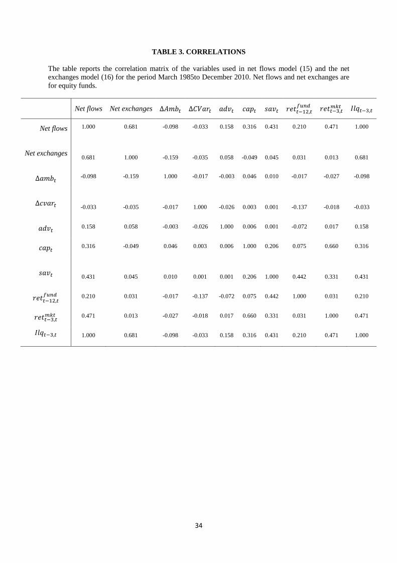
over the period March 1985 to December 2010. Table 3 reports the correlations between the variables,

and we can see that the changes in ambiguity series is negatively correlated with both net fund flow

and net fund exchanges.

[Table 3 here]

The regression for net flows is given by:

where is the aggregate cost of print advertising across all funds divided by the previous year’s

total advertising cost, is the capital gains, is the personal savings rate,

is the

aggregate fund return of the previous year, is the return on the value-weighted CRSP index

over the last 3 months. is the average market illiquidity from the previous three months, and

, , , and are dummy variables that are equal to one in the respective month and

zero otherwise.

For net exchanges, we estimate a similar model, but exclude the savings variable and the

seasonal dummy variables. The model for net exchanges is therefore given by:

4. Results

In this section, we report the results of the empirical analysis. We first focus on the equity

asset class, and then consider the effects of ambiguity on non-equity fund flows and exchanges.

Finally, in the last part of the section, we conduct some robustness checks.

18

4.1 Ambiguity and Equity Fund Flows

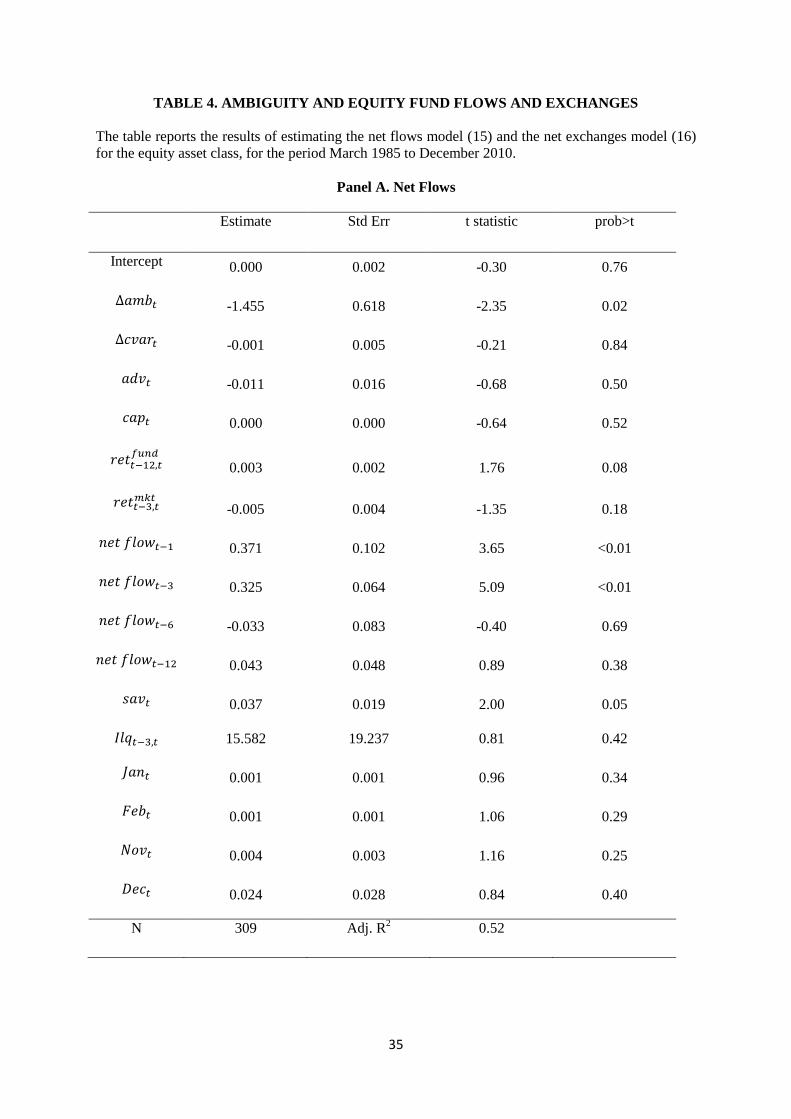
Panel A of Table 4 reports the results of estimating model (15) for net flows, for the equity

asset class. The coefficient on the change in ambiguity is negative and significant at conventional

levels (-1.455, p= 0.02). Therefore, in support of our hypothesis, an increase in ambiguity is

associated with a net outflow of capital from equity mutual funds. In contrast, changes in conditional

variance do not have a statistically significant impact on net flows (-0.001, p =0.84). The savings

variable has significantly positive coefficient (0.037, p=0.05), which is consistent with a “free cash

flow” effect on fund flows. Consistent with previous literature (Kamstra et al, 2011) lagged net fund

flows from the previous one and three months are positive and highly significant, showing strong

autocorrelation in flows. The remaining variables are not significant.

[Table 4 here]

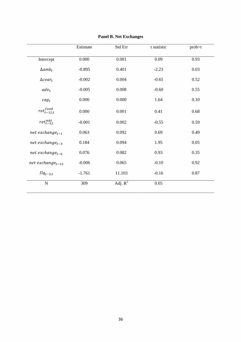
Panel B of Table 4 reports the estimation results from (16) for net exchanges for the equity

asset class. As with net flows, changes in ambiguity are negatively associated with net exchanges, and

this relationship is statistically significant (-0.895, p=0.03). Again, changes in risk have a negative but

insignificant impact (-0.002, p=0.52).14

The three month lag of net exchanges is positive and

statistically significant, reflecting strong autocorrelation in this series as well.

These results suggest that an increase in ambiguity has a negative and statistically significant

impact on net flows and net exchanges, supporting our hypothesis that increases in ambiguity lead to a

reduction in equity market participation. Moreover, while there is a clear link between ambiguity and

net fund flows and exchanges, the impact of risk is negative but not statistically significant. These

results are consistent with Anderson, Ghysels and Juergens (2009), who show that excess market

returns have a strong positive association with ambiguity, but a much weaker association with

conditional variance, and broadly imply that investors’ risk aversion is dominated by their ambiguity

aversion.

14

We have experimented with alternative measures of risk, including realized variance and realized excess

variance. The results show that risk remains insignificant but our conclusion about ambiguity holds regardless

the risk measure.

19

To gauge the economic significance of our results note that the standard deviation of the

ambiguity measure is 0.0013 and the average total net assets for equity funds is $1.9trillion;

consequently, a one standard deviation change in ambiguity will on average yield a net flow of $3.3

billion and a net exchange of $2.2 billion.

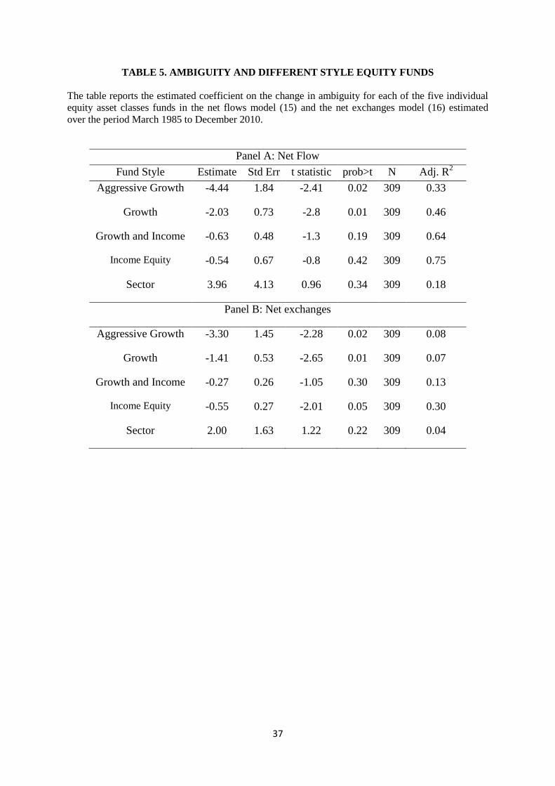
4.2 Ambiguity and Different Equity Styles

The results in the previous section show that ambiguity adversely affects overall stock market

participation. However, since ambiguity varies across equities (see Kelsey et al, 2010; Brenner and

Izhakian, 2011; Antoniou, Galariotis and Read, 2012), this effect will be more pronounced among

funds that invest in more ambiguous stocks. In this section we test this hypothesis by investigating

the relationship between ambiguity and fund flows for the five investment objective categories

separately, namely ‘aggressive growth’, ‘growth’, ‘sector’, ‘growth and income’ and ‘income equity’.

According to the ICI definition, aggressive growth and growth funds invest in riskier, non-dividend

paying stocks with a focus on capital gains. Conversely, funds in the remaining three categories focus

on less risky, dividend-paying stocks (ICI Factbook, 2012).

Dividend policy is a signal about the stability of the expected profitability of the firm. This is

because firms, being concerned with the penalties associated with dividend omissions (e.g., Michaely,

Thaler and Womack, 1995), tend to initiate and pay dividends when they reach a mature stage in their

life cycle and thus expect to be able to consistently make these payouts in the future.15

Conversely,

firms that do not pay dividends are typically those with significant growth opportunities, and it is

often quite challenging to foresee how these opportunities will develop. Therefore, on average,

ambiguity is considerably higher for non-dividend payers, which in turn implies that the effect of

ambiguity will be stronger among the aggressive growth and growth categories.16

15

For example Denis and Osobov (2008) show that dividend payers tend to be larger and more profitable

companies. 16

Bossaerts et al (2010) also note that growth companies entail significant ambiguity.

20

The results for net flows are shown in Panel A of Table 5. For brevity, the table reports only

the estimated coefficient on the change in ambiguity. For the ‘aggressive growth’ and ‘growth’

categories, the coefficient on the change in ambiguity is negative and highly statistically significant.

For the ‘growth and income’ and ‘income equity’ categories, the coefficient is negative but not

significant, while for the ‘sector’ category, the coefficient is insignificantly positive. The results for

net exchanges are broadly similar, as shown by Panel B of Table 5. Therefore, while our earlier

results show that an increase in ambiguity leads to flows and exchanges out of the equity asset class as

a whole, we can see that within the equity asset class, the effect is concentrated in the funds that invest

in more ambiguous, non-dividend paying assets.17

(Table 5 here)

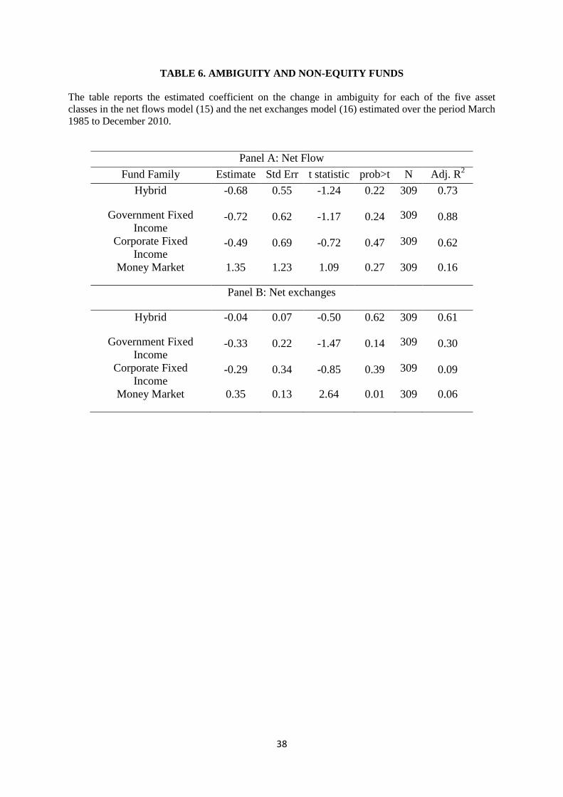
4.3 Ambiguity and non-Equity Fund Flows

In this section we examine the relationship between changes in ambiguity and flows in funds

that invest in non-equity asset classes, namely hybrid, government and corporate fixed income and

money market. It is reasonable to expect that in response to an increase in ambiguity in the stock

market, investors will transfer funds into less ambiguous, non-equity investments.

Panel A (B) of Table 6 reports the estimated coefficient on the change in ambiguity from the

net flows (exchanges) model. For net flows the coefficients on ambiguity are not significantly

different from zero. For net exchanges, however, the coefficient for the money market asset class is

positive and significant. Thus, as ambiguity increases, investors withdraw capital from equity funds

and reinvest, at least partially, in money market funds. According to the ICI definition, money market

funds invest in low risk, high-grade assets that will receive full principal and interest within 90 days

on average. Since our ambiguity measure is based on the stock market’s forecast of long-term growth,

one possible explanation for this finding is that investors are seeking safer assets with higher liquidity

when faced with higher ambiguity in expected stock returns.

17

The variables that control for aggregate market characteristics (i.e., risk, returns and liquidity) are the same as

those in the baseline model because ICI does not provide details on holdings.

21

[Table 6 here]

4.4 Ambiguity and Short Selling

In our theoretical exposition we have assumed that the ambiguity-averse agent always expects

positive returns on the risky asset, and showed that in the presence of ambiguity he assumes a long

position, which is smaller compared to the ambiguity-neutral case. This assumption is motivated by

the fact that in our empirical analysis we measure participation via mutual funds, which most

commonly do not take short positions.18

However, there is a caveat: it is possible that our previous analysis is only picking up a bias in

beliefs, whereby pessimistic EU (not ambiguity averse) agents withdraw their long positions, and at

the same time initiate short positions, so overall market participation does not change in response to

ambiguity. Although this explanation is unlikely19

we conduct some analysis in this section to

formally rule it out. Thus, we correlate a measure for the level of short selling activity in the market

with our ambiguity proxy. Using data from Compustat we calculate the aggregate value-weighted

short ratio (numbers of shares held shortt / number of shares outstanding at timet), and then correlate

the change in this variable with our measure of ambiguity. In unreported analysis we find that the

correlation is -0.127 (p=0.02), which suggests that increases in ambiguity reduce short positions in the

stock market. So overall, increases in ambiguity lead to reductions in both long and short positions in

the stock market, as predicted by the theoretical literature (i.e., Dow and Werlang, 1992; Epstein and

Schneider, 2010).

18

In more formal models of ambiguity like Dow and Werlang (1992) and Epstein and Schneider (2010), where

expected returns for the risky asset can be either positive or negative, agents can be either long or short.

Ambiguity aversion has opposite effects in these cases: when the agent is long his pessimism leads him to

expect low returns, and when he is short to expect high returns. For certain parameters for ambiguity these

models produce situations where the agent is neither long nor short. 19

Firstly, as we have discussed, fund flows reflect the active reallocation decisions of individual investors, and it

is well documented in the literature that these investors are reluctant to sell-short (Barber and Odean, 2008).

Secondly, it would be difficult to explain why these investors delegate decisions to go long to mutual funds

managers, but feel able to handle short positions on their own.

22

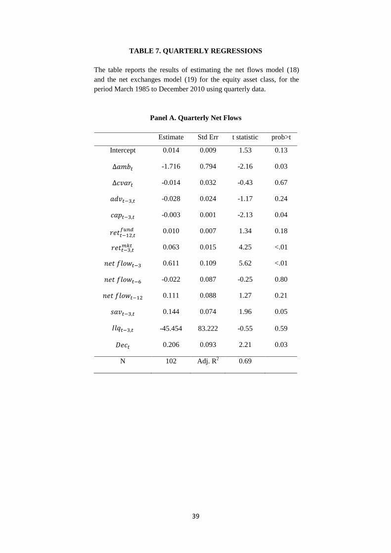
4.5 Robustness

As discussed in our methodology section we use linear interpolation for the ambiguity

measure to obtain monthly estimates and hence increase the power of our tests. In this section we

estimate the models shown in (15) and (16) using non-interpolated, quarterly data. We continue to use

Newey and West (1987, 1994) heteroscedasticity and autocorrelation consistent standard errors.

Net flows and exchanges are calculated on a quarterly basis. The changes in

ambiguity and conditional variance are equal to

, respectively. Quarterly capital gains, savings and advertising costs are equal to

the sum of the monthly values over each quarter: ,

and . Lagged market return, illiquidity premium and fund return are

defined as previously. The quarterly regressions are of the form:

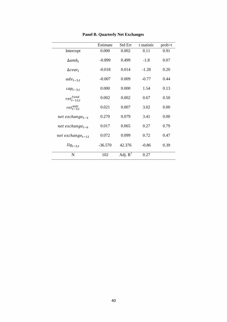
The results for these quarterly regressions are shown in Table 7. Even though the number of

observations in these models is reduced threefold, we still find that increases in ambiguity are

negatively and significantly related to both fund flows (Panel A: -1.716, p=0.03) and fund exchanges

(Panel B:-0.899, p=0.07).

[Table 7 here]

23

5. Conclusion

Limited stock market participation is a longstanding puzzle in finance and many explanations

have been put forward, including frictions-based and behavioural explanations. In this paper we

empirically test one prominent behavioural explanation, namely that non-participation is due to

ambiguity aversion. According to the ambiguity-based explanation, stocks involve both risk and

ambiguity, and since investors are ambiguity averse, their propensity to invest in stocks is lower than

that predicted by neoclassical models.

We measure market participation with flows of capital in and out of U.S. equity mutual funds.

Our measure of ambiguity is based on a recent study by Anderson, Ghysels and Juergens (2009) and

reflects the dispersion in analysts’ implied forecasts about market returns. Our results show that,

controlling for other factors that affect fund flows, increases in ambiguity are significantly negatively

related to equity fund flows and exchanges, and thus support the notion that limited stock market

participation arises because the stock market entails ambiguity, which is disliked by investors.

24

References

Ahn, D., S. Choice., D. Gale., and S. Kariv., 2011,‘Estimating ambiguity aversion in a portfolio

choice experiment’, working paper, UC Berkeley.

Allen, F. and D. Gale., 1994, ‘Limited market participation and volatility of asset prices’, American

Economic Review, 84, 933-955.

Amihud. Y., 2002, ‘Illiquidity and stock returns: cross-section and time-series effects’, Journal of

Financial Markets, 7, 31-56.

Anderson, E., E. Ghysels., and J. Juergens., 2009, ‘The impact of risk and uncertainty on expected

returns’, Journal of Financial Economics, 94, 233-263.

Antoniou, C., E.C. Galariotis., and D. Read., 2012, ‘Ambiguity aversion, company size and the

pricing of earnings forecasts’, European Financial Management, forthcoming.

Banerjee, S., B. Green., 2012, ‘Learning whether other traders are informed’, working paper,

Northwestern University

Barber, B., and T. Odean, 2008, ‘All that glitters: The effect of attention and news on the buying

behaviour of individual and institutional investors’, Review of Financial Studies, 21, 785-818.

Ben-Rephael, A.,S. Kandel., and A. Wohl., 2012, ‘Measuring investor sentiment with mutual fund

flows’, Journal of Financial Economics, 104, 363-382.

Ben-Rephael, A., S. Kandel., and A. Wohl., 2011, ‘The price pressure of aggregate mutual fund

flows’, Journal of Financial and Quantitative Analysis, 46, 585-603.

Bossaerts, P., Ghirardato, P., Guarnaschelli, S., and Zame,W., 2010,‘Ambiguity in asset markets:

theory and experiment’, Review of Financial Studies, 23,1325-59

Brenner, M., and Y. Izhakian, 2011, ‘Asset pricing and ambiguity: Empirical Evidence’, working

paper, New York University.

Camerer, C., and H. K. Kunreuther, 1989,‘Experimental markets for insurance’, Journal of Risk and

Uncertainty, 2, 265-300.

Campbell, J., 2006, ‘Household Finance’, Journal of Finance, 4, 1553-1603.

25

Cao, H., T. Wang and H. Zhang, 2005, ‘Model uncertainty, limited market participation and asset

prices’, Review of Financial Studies, 18, 1219–1251.

Caskey, J., 2009, ‘Information in equity markets with ambiguity-averse investors’, Review of

Financial Studies, 22, 3595-3627.

Cooper, M.J., Gulen, H. and Rau, P.R., 2005, ‘Changing names with style: mutual fund name changes

and their effects on fund flows.’ Journal of Finance, 60, 2825-2858.

Collard, F., S. Mukerji, K. Sheppard.,and J. Tallon., 2011, ‘Ambiguity and the historical equity

premium’, working paper, University of Oxford.

Chen, Z., and L.G. Epstein., 2002, ‘Ambiguity, risk and asset returns in continuous time’,

Econometrica, 70, 190-200.

Denis, D., J., and Osobov, I., 2008, ‘Why do firms pay dividends? International evidence on the

determinants of dividend policy’, Journal of Financial Economics, 89, 62-82.

Dow, J., and S. Werlang., 1992, ‘Ambiguity aversion, risk aversion, and the optimal choice of

portfolio’, Econometrica, 60, 197–204.

Drechsler, I., 2012, ‘Uncertainty, time-varying fear, and asset prices’, Journal of Finance,

forthcoming.

Einhorn, J. H. and M. R. Hogarth, 1985, ‘Ambiguity and uncertainty in probabilistic inference’,

Psychological Review, 92, 433-462.

Epstein, L., and T. Wang., 1994, ‘Intertemporal asset pricing under Knightian ambiguity’,

Econometrica, 62, 283–322.

Epstein, L., and M. Schneider., 2008, ‘Ambiguity, information quality, and asset pricing’, Journal of

Finance, 63, 197-228.

Epstein, L., and M. Schneider., 2010, ‘Ambiguity and asset market’, Annual Review of Financial

Economics, 2, 315-346.

Easley, D., and M. O’Hara, 2009, ‘Ambiguity and nonparticipation: the role of regulation’, Review of

Financial Studies, 22, 1817–43.

Ellsberg, D., 1961, ‘Risk, ambiguity, and the Savage axioms’, Quarterly Journal of Economics,

75 ,643– 669.

26

Frisch, D. And J. Baron, 1988, ‘Ambiguity and Rationality’, Journal of Behavioral Decision Making,

1, 149-157.

Gärdenfors, P. And N. E. Sahlin, 1982, ‘Unreliable Probabilities, risk taking, and decision making’,

Synthese, 361-386.

Gärdenfors, P. And N. E. Sahlin, 1983, ‘Decision Making with Unreliable Probabilities’, British

Journalof Mathematical and Statistical Psychology, 36, 1983, 240-251.

Gallaher, S., R. Kaniel, and L. Starks., 2006, ‘Mutual funds and advertising, mimeo’, working paper,

University of Texas at Austin.

Gilboa, I., and Schmeidler D., 1989, ‘Maxmin expected utility with non-unique prior’, Journal of

Mathematical Economics, 18, 141–153.

Guiso, L., M. Haliassos., and T. Jappelli., 2003, ‘Household stockholding in Europe: where do we

stand, and where do we go?’, working paper, Centre for Economic Policy Research.

Haliassos, M. and C. Bertaut., 1995, ‘Why do so few hold stocks?’, The Economic Journal, 105,

1110-1129.

Hong, H., J. D. Kubik., and J. C. Stein., 2004, ‘Social interaction and stock-market participation’,

Journal of Finance, 59, 137-163.

Hsu, J., 2012, ‘What drives equity market non-participation?’, North American Journal of Economics

and Finance, 23, 86-114.

Hsu, M., Bhatt, M., Adolphs, R., Tranel, D., Camerer, C. F., 2005, ‘Neural systems responding to

degrees of uncertainty in human decision-making’, Science, 310, 1680-1683.

Investment Company Institute, 2012, Investment Company Fact Book: A Review of Trends and

Activity in the U.S. Investment Company Industry, 52nd Edition.

Investment Company Institute, 2003, Mutual Fund Fact Book: A Guide to Trends and Statistics in the

Mutual Fund Industry, 43rd Edition.

Ippolito, R.A., 1992, ‘Consumer reaction to measures of poor quality: evidence from the mutual fund

industry’, Journal of Law and Economics, 35, 45-70.

Ivkovich. Z., and Weisbenner. S., 2009, ‘Individual Investor Mutual-Fund Flows.’ Journal of

Financial Economics, 92, 223-237.

27

Jain, C. & Wu, S., 2000, ‘Truth in mutual fund advertising: evidence of future performance and fund

flows’, Journal of Finance, 55, 937-958.

Kacperczyk, M, and Seru. A., 2007, ‘Fund manager use of public information: new evidence on

managerial skills’, Journal of Finance 62, 485-528.

Kamstra, M.J., L.A. Kramer, M.D. Levi, and R. Wermers, 2011, ‘Seasonal asset allocation: evidence

from mutual fund flows’, working paper, University of Toronto.

Keynes, J., 1921, A Treatise on Probability, Cornell University Library, New York.

Kelsey, D., R. Kozhan., and W. Pang., 2008, ‘Asymmetric momentum effects under uncertainty’,

Review of Finance, 15, 603-631.

Keren, G. B., and Gerritsen, L. E. M., 1999, ‘On the robustness and possible accounts for ambiguity

aversion’, Acta Psychologica, 103, 149–172.

Klibanoff. P., Marinacci M., and Mukerji. S., 2005, ‘A smooth model of decision making under

ambiguity’, Econometrica, 73, 1849-1892

Knight, F.H., 1921, Risk, Uncertainty and Profit, Houghton Mifflin Company, Boston, MA.

Levy I., Snell J., Nelson AJ.,Rustichini A., Glimcher P., 2010, ‘The neural representation of

subjective value under risk and ambiguity’, Journal of Neurophysiology, 103, 1036-1047.

Maccheroni, F., M.Marinacci., and A. Rustichini., 2006, ‘Ambiguity aversion, robustness, and the

variational representation of preferences’, Econometrica, 74, 1447-1498.

Mehra, R., 2003, ‘The equity premium: Why is it a puzzle?’, Financial Analysts Journal, 59, 54-69.

Mehra, R., and E. C. Prescott., 1985, ‘The equity premium: a puzzle’, Journal of Monetary

Economics, 15, 145–161.

Michaely, R., R. H. Thaler, and K. L. Womack, 1995, ‘Price reactions to dividend initiations and

omissions: Overreaction or drift?’, Journal of Finance, 50, 573-608.

Mukerji, S., and J.-M. Tallon., 2001, ‘Ambiguity aversion and incompleteness of financial markets,’

Review of Economic Studies, 68, 883-904.

Newey, W. K. and K. D. West, 1987, ‘A simple positive semi-definite heteroscedasticity and

28

autocorrelation consistent covariance matrix’, Econometrica, 55, 703-708.

Newey, W.K. and K.D. West., 1994, ‘Automatic lag selection in covariance matrix estimation’,

Review of Economic Studies, 61, 631-653.

Sarin, R.K., and M. Weber., 1993, ‘Risk-Value Models.’ European Journal of Operational Research

70, 135 – 149.

Savage, L.J., 1954, The Foundations of Statistics, New York: John Wiley.

Sirri, E., and P. Tufano, 1998, ‘Costly search and mutual fund flows’, Journal of Finance, 53,1589–

1622.

Takashi, U., 2011, ‘The ambiguity premium vs. the risk premium under limited market participation’,

Review of Finance, 15, 245-275.

Vissing-Jorgenson, A., 2002, ‘The returns to entrepreneurial investment: a private equity premium

puzzle?’, American Economic Review, 92, 745-778.

Werner, J., 2001, ‘Participation in risk-sharing under ambiguity’, working paper, University of

Minnesota.

Williamson. S., 1994, ‘Liquidity and Market Participation’, Journal of Economic Dynamics and

Control, 18, 629-670.

29

FIGURE 1. NET FLOWS AND NET EXCHANGES FOR THE EQUITY ASSET CLASS

The figure reports the monthly net flows and net exchanges for the equity asset class, which

comprises funds within the ‘aggressive growth’, ‘growth’, ‘sector’, ‘growth and income’, and ‘income

equity’ investment objective categories. The data is from ICI and covers the period March 1985to

December 2010. Net flows (reported in Panel A) and net exchanges (reported in Panel B) are

calculated according to Equations (6) and (7).

Panel A. Net Flows

Panel B. Net Exchanges

-0.03

-0.02

-0.01

0

0.01

0.02

0.03

0.04

01-Jan-85 01-Jan-90 01-Jan-95 01-Jan-00 01-Jan-05 01-Jan-10

Net flow

-0.025

-0.02

-0.015

-0.01

-0.005

0

0.005

0.01

0.015


Net exchanges

30

FIGURE 2. AMBIGUITY

The figure reports quarterly ambiguity and the change in monthly ambiguity, from 1985 to 2010.

Quarterly ambiguity is calculated using Equation (12) with v=15.346. Monthly ambiguity is computed

from the quarterly measure by linear interpolation. Both series are scaled by 100. Panel A reports

quarterly ambiguity, and Panel B reports the change in monthly ambiguity. The forecast data is from

http://www.phil.frb.org/econ/spf/index.html.

Panel A. Quarterly Ambiguity

Panel B. Changes in Monthly Interpolated Ambiguity

0

0.002

0.004

0.006

0.008

0.01


Ambiguity

-0.003

-0.002

-0.001

0

0.001

0.002

0.003


ΔAmbiguity

http://www.phil.frb.org/econ/spf/index.html

31

FIGURE 3. AMBIGUITY VS. RISK

The figure reports monthly ambiguity (solid line) and conditional variance (dashed line) from March

1985to December 2010. Conditional variance is calculated using Equation (14). The raw data is from

CRSP. For comparison, ambiguity has been scaled by 5000.

0

0.1

0.2

0.3

0.4

0.5

0.6


Ambiguity & Risk

32

TABLE 1. CLASSIFICATION OF U.S. MUTUAL FUNDS

The table reports the categorisation of the ICI fund investment objective categories by asset class,

based on Kamstra et al. (2011).

Fund Investment Objective Fund Asset Class

Aggressive Growth Equity

Growth Equity

Sector Equity

Growth and Income Equity

Income Equity Equity

Asset Allocation Hybrid

Balanced Hybrid

Flexible Portfolio Hybrid

Income Mixed Hybrid

Corporate - General Corporate Fixed Income

Corporate - Intermediate Corporate Fixed Income

Corporate - Short Term Corporate Fixed Income

High Yield Corporate Fixed Income

Strategic Income Corporate Fixed Income

Government Bond - General Government Fixed Income

Government Bond - Intermediate Government Fixed Income

Government Bond - Short Term Government Fixed Income

Mortgage Backed Government Fixed Income

State Municipal Bond - General Government Fixed Income

State Municipal Bond - Short Term Government Fixed Income

National Municipal Bond - General Government Fixed Income

National Municipal Bond - Short Term Government Fixed Income

Taxable Money Market - Government Money Market

33

TABLE 2. SUMMARY STATISTICS

The table reports summary statistics for the monthly net flows and net exchanges for the domestic

equity funds group, ambiguity and changes in ambiguity and the control variables for the period

March 1985to December 2010. is ambiguity and is conditional variance, and are

calculated according to equations (12) and (14), respectively. Ambiguity is scaled by 100. − −1 and ∆ = − −1. is the aggregate cost of print advertising across

all funds, divided by the previous year’s total advertising cost, is the capital gains in month t,

from Kamstra et al. (2011) Table 1. is the personal savings rate taken from the Bureau of

Economic Analysis (series PSAVERT).

is the aggregate return of equity funds over the

previous 12 months. is the return on the CRSP value-weighted index (series VWRETD) over

the last 3 months and is the Amihud liquidity measure of previous three months.

Mean Std Skew Kurt Max Min

Net exchanges -0.00040 0.00271 -2.14912 13.95975 0.00963 -0.02098

Net flow 0.00505 0.00706 0.24226 1.69242 0.03465 -0.02345

0.00158 0.00129 1.79998 4.20630 0.00800 0.00017

-0.00001 0.00052 0.29638 5.99293 0.00245 -0.00213

0.03228 0.05060 5.49622 38.66370 0.48476 0.00259

0.00007 0.04326 4.82699 61.81308 0.45413 -0.27649

0.16747 0.21849 -0.96633 0.86778 0.58296 -0.58001

0.08600 0.01240 0.81052 5.93306 0.14438 0.03810

8.40841 19.44562 2.93770 6.82710 72.00000 0.90000

0.04935 0.01889 0.00658 -0.80069 0.10300 0.00900

0.02761 0.08464 -1.07597 2.85516 0.26384 -0.36722

0.00002 0.00001 3.01512 14.23607 0.00009 0.00000

34

TABLE 3. CORRELATIONS

The table reports the correlation matrix of the variables used in net flows model (15) and the net

exchanges model (16) for the period March 1985to December 2010. Net flows and net exchanges are

for equity funds.

Net flows Net exchanges

Net flows 1.000 0.681 -0.098 -0.033 0.158 0.316 0.431 0.210 0.471 1.000

Net exchanges 0.681 1.000 -0.159 -0.035 0.058 -0.049 0.045 0.031 0.013 0.681

-0.098 -0.159 1.000 -0.017 -0.003 0.046 0.010 -0.017 -0.027 -0.098

-0.033 -0.035 -0.017 1.000 -0.026 0.003 0.001 -0.137 -0.018 -0.033

0.158 0.058 -0.003 -0.026 1.000 0.006 0.001 -0.072 0.017 0.158

0.316 -0.049 0.046 0.003 0.006 1.000 0.206 0.075 0.660 0.316

0.431 0.045 0.010 0.001 0.001 0.206 1.000 0.442 0.331 0.431

0.210 0.031 -0.017 -0.137 -0.072 0.075 0.442 1.000 0.031 0.210

0.471 0.013 -0.027 -0.018 0.017 0.660 0.331 0.031 1.000 0.471

1.000 0.681 -0.098 -0.033 0.158 0.316 0.431 0.210 0.471 1.000

35

TABLE 4. AMBIGUITY AND EQUITY FUND FLOWS AND EXCHANGES

The table reports the results of estimating the net flows model (15) and the net exchanges model (16)

for the equity asset class, for the period March 1985 to December 2010.

Panel A. Net Flows

Estimate Std Err t statistic prob>t

Intercept 0.000 0.002 -0.30 0.76

-1.455 0.618 -2.35 0.02

-0.001 0.005 -0.21 0.84

-0.011 0.016 -0.68 0.50

0.000 0.000 -0.64 0.52

0.003 0.002 1.76 0.08

-0.005 0.004 -1.35 0.18

0.371 0.102 3.65 <0.01

0.325 0.064 5.09 <0.01

-0.033 0.083 -0.40 0.69

0.043 0.048 0.89 0.38

0.037 0.019 2.00 0.05

15.582 19.237 0.81 0.42

0.001 0.001 0.96 0.34

0.001 0.001 1.06 0.29

0.004 0.003 1.16 0.25

0.024 0.028 0.84 0.40

N 309 Adj. R2 0.52

36

Panel B. Net Exchanges


Intercept 0.000 0.001 0.09 0.93

-0.895 0.401 -2.23 0.03

-0.002 0.004 -0.65 0.52

-0.005 0.008 -0.60 0.55

0.000 0.000 1.64 0.10

0.000 0.001 0.41 0.68

-0.001 0.002 -0.55 0.59

0.063 0.092 0.69 0.49

0.184 0.094 1.95 0.05

0.076 0.082 0.93 0.35

-0.006 0.065 -0.10 0.92

-1.761 11.103 -0.16 0.87

N 309 Adj. R2 0.05

37

TABLE 5. AMBIGUITY AND DIFFERENT STYLE EQUITY FUNDS

The table reports the estimated coefficient on the change in ambiguity for each of the five individual

equity asset classes funds in the net flows model (15) and the net exchanges model (16) estimated

over the period March 1985 to December 2010.

Panel A: Net Flow

Fund Style Estimate Std Err t statistic prob>t N Adj. R2

Aggressive Growth -4.44 1.84 -2.41 0.02 309 0.33

Growth -2.03 0.73 -2.8 0.01 309 0.46

Growth and Income -0.63 0.48 -1.3 0.19 309 0.64

Income Equity -0.54 0.67 -0.8 0.42 309 0.75

Sector 3.96 4.13 0.96 0.34 309 0.18

Panel B: Net exchanges

Aggressive Growth -3.30 1.45 -2.28 0.02 309 0.08

Growth -1.41 0.53 -2.65 0.01 309 0.07

Growth and Income -0.27 0.26 -1.05 0.30 309 0.13

Income Equity -0.55 0.27 -2.01 0.05 309 0.30

Sector 2.00 1.63 1.22 0.22 309 0.04

38

TABLE 6. AMBIGUITY AND NON-EQUITY FUNDS

The table reports the estimated coefficient on the change in ambiguity for each of the five asset

classes in the net flows model (15) and the net exchanges model (16) estimated over the period March

1985 to December 2010.

Panel A: Net Flow

Fund Family Estimate Std Err t statistic prob>t N Adj. R2

Hybrid -0.68 0.55 -1.24 0.22 309 0.73

Government Fixed

Income -0.72 0.62 -1.17 0.24 309 0.88

Corporate Fixed

Income -0.49 0.69 -0.72 0.47 309 0.62

Money Market 1.35 1.23 1.09 0.27 309 0.16

Panel B: Net exchanges

Hybrid -0.04 0.07 -0.50 0.62 309 0.61

Government Fixed

Income -0.33 0.22 -1.47 0.14 309 0.30

Corporate Fixed

Income -0.29 0.34 -0.85 0.39 309 0.09

Money Market 0.35 0.13 2.64 0.01 309 0.06

39

TABLE 7. QUARTERLY REGRESSIONS

The table reports the results of estimating the net flows model (18)

and the net exchanges model (19) for the equity asset class, for the

period March 1985 to December 2010 using quarterly data.

Panel A. Quarterly Net Flows


Intercept 0.014 0.009 1.53 0.13

-1.716 0.794 -2.16 0.03

-0.014 0.032 -0.43 0.67

-0.028 0.024 -1.17 0.24

-0.003 0.001 -2.13 0.04

0.010 0.007 1.34 0.18

0.063 0.015 4.25 <.01

0.611 0.109 5.62 <.01

-0.022 0.087 -0.25 0.80

0.111 0.088 1.27 0.21

0.144 0.074 1.96 0.05

-45.454 83.222 -0.55 0.59

0.206 0.093 2.21 0.03

N 102 Adj. R2 0.69

40

Panel B. Quarterly Net Exchanges


Intercept 0.000 0.002 0.11 0.91

-0.899 0.499 -1.8 0.07

-0.018 0.014 -1.28 0.20

-0.007 0.009 -0.77 0.44

0.000 0.000 1.54 0.13

0.002 0.002 0.67 0.50

0.021 0.007 3.02 0.00

0.270 0.079 3.41 0.00

0.017 0.065 0.27 0.79

0.072 0.099 0.72 0.47

-36.570 42.376 -0.86 0.39

N 102 Adj. R2 0.27

ambiguity aversion and stock market participation

Documents