Ambiguity, Monetary Policy and Trend Inflation∗

Riccardo M. Masolo Francesca Monti

Bank of England and CfM

September 9, 2016

Abstract

We build a model that can explain the evolution of trend inflation in the US as a

function of the changes in the private sector’s confidence in their understanding of the

monetary policymaker’s behavior, measured by the dispersion in the individual SPF now-

casts of the 3-month T-Bill rate. Rather than resorting to exogenous changes in the

inflation target process, the model features ambiguity-averse agents and ambiguity re-

garding the conduct of monetary policy. Ambiguity turns out to be key in explaining the

difference between the inflation target pursued by the central bank and the inflation trend

measured in the data.

JEL Classification: D84, E31, E43, E52, E58

Keywords: Ambiguity aversion, monetary policy, trend inflation

1 Introduction

The dynamics of inflation and, in particular, its persistence are driven in large part by

a low-frequency, or trend, component, as documented for example in Stock and Watson

(2007) and Cogley and Sbordone (2008). Most of the macroeconomic literature relies,

however, on models that are approximated around a zero-inflation steady state1 and that,

consequently, cannot capture the persistent dynamic properties of inflation. Positive

∗Previously circulated as Monetary Policy with Ambiguity Averse Agents. We are grateful to Guido Ascari,Carlos Carvalho, Ferre DeGraeve, Jesus Fernandez-Villaverde, Richard Harrison, Cosmin Ilut, Peter Karadi andWouter Den Haan for insightful comments and suggestions. We would also like to thank seminar participantsat Oxford University, Bank of Finland, ECB-WGEM, Bank of Korea, Bank of England, Bank of Canada andKing’s College London, as well as participants at the 2015 North American Winter Meeting of the EconometricSociety, 2015 SNDE, the XVII Inflation Targeting Conference at BCDB, Barcelona GSE summer forum and the2015 EEA conference. Any views expressed are solely those of the authors and so cannot be taken to representthose of the Bank of England or to state Bank of England policy. This paper should therefore not be reportedas representing the views of the Bank of England or members of the Monetary Policy Committee or FinancialPolicy Committee.

1Or alternatively, and equivalently from this perspective, a full indexation steady-state.

1

steady-state inflation also has far-reaching effects on the static and dynamic properties of

the model (see Ascari and Sbordone, 2014, for an overview), including a dramatic impact

on the lowest degree of inflation responsiveness that can ensure equilibrium determinacy,

as highlighted in Coibion and Gorodnichenko (2011). It is therefore crucial to have models

that can account for trend inflation and its dynamics.

In order to capture the dynamics of inflation, Del Negro and Eusepi (2011) and Del Ne-

gro, Giannoni and Schorfheide (2015) propose replacing the constant inflation target with

a time-varying very persistent but otherwise exogenous inflation target process. While

this assumption helps match the data better, it does not provide a compelling explanation

for the low frequency movements in inflation. We argue, in fact, that the assumption of an

exogenous slow-moving inflation target is counterfactual. While the Federal Reserve only

explicitly adopted an inflation target in 2012, we have reasons to believe, as we illustrate

in Section 2, that inflation targets had been more or less implicitly in place long before

that. Moreover, if inflation targets vary at all, they do so in a discrete and infrequent

fashion and do not represent the same concept as trend inflation.

In this paper, we present a simple model that can explain the persistent differences

between target and trend inflation. The key driver of this wedge is a time-varying degree

of private sector’s confidence in the conduct of monetary policy, which we model as am-

biguity about the monetary policy rule. Ambiguity describes a situation in which there is

uncertainty about the probability distribution over states of the world: agents entertain

as possible not one but a set of beliefs and they are unable to assign probabilities to each

of them. We augment a prototypical new-Keynesian model by 1) introducing ambiguity

about the monetary policy rule and 2) assuming that agents are averse to ambiguity.

We introduce ambiguity aversion in the model using a recursive version of the multiple

prior preferences (see Gilboa and Schmeidler, 1989, and Epstein and Schneider, 2003),

pioneered in business cycle models by Ilut and Schneider (2014).

Ambiguity-averse agents will base their decisions on the worst-case scenario consistent

with their belief set. In practice, in our model agents base their decisions on a distorted

belief about the interest rate, which differs from the one actually set by the central bank.

As a result, inflation in steady state does not necessarily coincide with the target. Our

model delivers a characterization of the relationship between inflation trend and target,

which depends on the degree of ambiguity about monetary policy – that is on how wide

the private sector’s set of beliefs about the interest is – and the responsiveness of the

policy rate to inflation. To keep things simple and implications stark, we work under the

assumption that the policy response function followed by the Fed never changed over the

35-year period we consider. The observed changes in the behavior of inflation (both at

high and low frequency) are, therefore, the result of differing degrees of confidence the

private sector has in the Fed’s policy.

With a very standard calibration and using data on the dispersion of interest rate

nowcasts available in the Survey of Professional Forecasters as a measure for ambiguity

about monetary policy, our model can explain the dynamics of trend inflation in the

US since the early 1980s (the beginning of our sample) without resorting to exogenous

changes in the inflation target. The model can match the dynamics of trend inflation

2

in the period before the Great Recession, when trend inflation was mostly above target

but falling, as well as the low trend inflation of the post-crisis period.2 We show that,

before the crisis, the worst-case scenario was one in which the private sector feared that

the interest rate would be lower than implied by the actual policy rule, thus resulting

in above-target inflation. Our model explains the recent low level of trend inflation as

a consequence of the proximity of the policy rate to the zero lower bound, which sets a

floor to the distortion of the beliefs about the interest rate. If the asymmetry generated

by the zero lower bound is large enough, then agents will make their consumption-saving

decision based on a distorted belief that the interest rate is above the one actually set by

the central bank, and this will generate lower inflation.

Our work can also explain the switch from indeterminacy to determinacy during the

early years of the Volcker chairmanship without resorting to changes in the responsiveness

of policy to inflation, in line with Coibion and Gorodnichenko (2012), or even to changes

in the target.

The rest of the paper is organized as follows. In section 2 we discuss whether assuming

a constant inflation target is a reasonable characterisation of the definition of the price

stability part of the Fed’s dual mandate and we present evidence regarding changes in

confidence about the conduct of monetary policy and the plausible link with increases

in transparency. Section 3 provides a description of the model we use for our analysis,

characterizes the steady state of our economy as a function of the degree of ambiguity and

studies optimal monetary policy in the presence of ambiguity. In Section 4 we show how

our simple model can match the dynamics of trend inflation, while Section 5 concludes.

2 Empirical and narrative evidence

In this Section we first discuss evidence on the low-frequency component of inflation. We

then present evidence in support of our claim that these low frequency movements do not

seem to be driven by variations in the inflation target. Finally we discuss how measures of

confidence about the conduct of monetary policy instead have been increasing, plausibly

linked to the increases in transparency over the last three decades.

Trend inflation and the inflation target A vast number of papers propose esti-

mates of trend inflation based on different models.3 And invariably, they have all declined

since the early 1980s, as a result of the fall in headline inflation. We take as benchmark

the estimate of trend inflation we obtain with a bayesian vector autoregression model with

drifting coefficients, along the lines of Cogley and Sargent (2002). In particular we use the

specification presented in Cogley and Sbordone (2008), using the same four data series:

implicit GDP deflator, real GDP growth, unit labor cost to approximate a measure of

marginal cost, and the fed funds rate on a discount basis. Figure 1 reports it, along with

the mean inflation over the sample and the 90% confidence bands. Clearly, inflation is

2There is some evidence that trend inflation might have fallen below 2% since 2009-2010, according toseveral measures shown in Garciga (2016).

3See for example Clark and Doh (2013) for a review of the main models in use and their relative forecastingperformance.

3

Figure 1: Inflation, mean inflation and trend inflation

1960 1970 1980 1990 2000 2010

0

0.02

0.04

0.06

0.08

0.1

InflationMean InflationTrend Inflation

characterized by a trend component, which has fallen since the early 1980s and is cur-

rently estimated to be slightly below target. The aim of our paper is to show how it is

possible to match its dynamics without resorting to an exogenous inflation target shock.

Models that explain the dynamics of inflation with exogenous variation in the infla-

tion target seem at odds with evidence from various sources, including the Blue Book,

a document about monetary policy alternatives presented to the committee by Fed staff

before each FOMC meeting. While the Federal Reserve officially did not have a target

value for inflation until 2012, the Blue Book simulations have been produced assuming

targets of 1.5% and 2% since at least 2000. In his book “A Modern History of FOMC

Communication: 1975-2002”, Lindsey (2003) states that, as early as July 1996, numerous

FOMC committee members had indicated at least an informal preference for an inflation

rate in the neighborhood of 2%, as indicated by FOMC transcripts.4 Goodfriend (2003)

provides detailed evidence that the Fed had implicitly adopted an inflation target in the

1980s, as this excerpt makes clear:

Chairman Greenspan testified in 1989 in favor of a qualitative zero inflation objective for

the Fed defined as a situation in which ”the expected rate of change of the general level of

prices ceases to be a factor in individual and business decisionmaking. Thus, it is reason-

able to think that the Greenspan Fed set out to achieve low enough inflation to make that

definition of price stability a reality. [...] This is the first sense in which it is plausible to

think that the Greenspan Fed has adopted an implicit form of inflation targeting.

Goodfriend (2003), p. 11

Indeed, Orphanides (2002) supports the view that the policy goal has not funda-

4See transcripts of the July 2-3, 1996, FOMC meeting for a statement by Chairman Greenspan.

4

mentally changed since at least World War II, and that low and stable inflation plays a

prominent role in its definition:

Did not the policymakers of the 1970s make a systematic effort to guide the economy

to its non-inflationary full employment potential? This, after all, had been and remains

the underlying macroeconomic policy objective of government policies in the United States

since at least the end of World War II.

Orphanides (2002), p. 1

In sum, it seems clear that the concept of inflation trend differs from that of inflation

target. We see the latter as changing, if at all, at few and relatively distant points in time,

while the former moves, albeit slowly, with every change in headline inflation. The rest

of this paper is primarily dedicated to explaining the wedge between trend inflation and

the target. In so doing we maintain a very conservative assumption that the target has

never changed over the period covered by our sample, which starts in the early 1980s.

Private sector confidence and transparency. The discussion above highlights

how the explicit announcement of an inflation target in 2012 can be seen as the culmi-

nation of a process geared towards greater transparency that started much earlier. The

main milestones in the Federal Reserve’s progress toward greater openness, according to

Lindsey’s (2003) detailed account of FOMC communication, include: in 1979, the first

release of semiannual economic projections; in 1983, the first publication of the Beige

Book, which summarizes information about economic conditions received from the Fed-

eral Reserve System’s business contacts; in 1994, the decision to release a postmeeting

statement when policy actions had been taken; in 2000, the beginning of the practice of

issuing a statement after each meeting of the Federal Open Market Committee (FOMC)

and including in the statement an assessment of the balance of risks to the Committee’s

objectives; and in 2002, adding the FOMC roll call vote to the postmeeting statements.

Transparency is key to boost the private sector’s confidence in the conduct of monetary

policy, as various papers demonstrate. Swanson (2006) shows that, since the late 1980s,

U.S. financial markets and private sector forecasters have become better able to forecast

the federal funds rate at horizons out to several months. Moreover, his work shows

that the cross-sectional dispersion of their interest rate forecasts shrank over the same

period and, importantly, also provides evidence that these phenomena can be traced

back to increases in central bank transparency. Ehrmann et al. (2012) also find that

increased central bank transparency lowers disagreement among professional forecasters.

This seems natural. For a given degree of uncertainty about the state of the economy,

improved knowledge about the policymakers’ objectives and model will help the private

sector anticipate policy responses more accurately. In other words, it translates into a

reduction of ambiguity about monetary policy. More recently Boyarchenko et al. (2016)

use high-frequency data on a wide range of asset yields and find evidence that FOMC

announcements affect the prices of risky assets not only directly by announcing changes

in Fed funds targets, but also indirectly by influencing the risk premium.

These findings are supported by statements by policymakers, clearly conveying the

idea that they saw increased transparency and communication as both necessary and ef-

5

Figure 2: A measure of disagreement about the interest rate

82 84 86 88 90 92 94 96 98 00 02 04 06 08 10 12 140

0.5

1

1.5

2

2.5

Year

Annualiz

ed P

erc

enta

ge P

oin

ts

The solid line is the interdecile dispersion of SPF nowcasts of the 3-month T-Bill rate. The three dotted verticallines indicate the various policy eras highlighted in Lindsey (2003) - 1982:1989 targeting borrowed reserves;1990-1999 targeting thefed funds rate; 2000-2008 the “era of communication” - and the period since the GreatRecession.

fective in helping the private sector anticipate policy moves:

... the faulty estimate was largely attributable to misapprehensions about the Fed’s inten-

tions. [...] Such misapprehensions can never be eliminated, but they can be reduced by a

central bank that offers markets a clearer vision of its goals, its ’model’ of the economy,

and its general strategy.

Blinder (1998)5

Our model will capture exactly this mechanism by explicitly considering that private

sector agents entertain multiple priors on the monetary policy rule, as a way of formalizing

the mishapprehensions Blinder (1998) refers to.

A separate question is how to measure ambiguity. We follow the bulk of the literature,

which takes forecast dispersion as a proxy for ambiguity (see for example Drechsler, 2013,

and Ilut and Schneider, 2014). Works such as those by Swanson (2006) and Ehrmann et

al. (2012) give us confidence that measuring ambiguity this way captures the gist of the

effects of increased transparency on the private sector’s understanding of monetary policy.

Our measure of changes in confidence, reported in Figure 2, is the dispersion of survey

of professional forecasters (SPF) nowcasts of the 3-month T-Bill rate, which are available

from 1981Q3 onward6. We take a 4-quarter moving average to smooth out very high-

frequency variations which would have not much to say about trends. But, clearly, the

scale of the numbers, which is really what we are primarily concerned with, is unaffected.

5Also reported by Coibion and Gorodnichenko (2012).6We experimented with Consensus data as well. Its dispersion is very similar to the one of the SPF in size

and dynamics, but Consensus data is available only from 1993 onward, while we are interested in extending thesample back as much as possible.

6

Unfortunately SPF data on the federal funds rate is, to our knowledge, only available

since the late 1990s, so we use the 3-month T-Bill rate as a proxy for the policy rate.

We evaluate the dispersion of the nowcasts rather than forecasts at further horizons,

because we aim to isolate the disagreement about monetary policy itself, rather than

about the realizations of key macroeconomic variables. The nowcasts are produced in the

middle of a quarter and thus incorporate a lot of information about the current state of

the economy. We compared our measure of ambiguity with a commonly used measure

of policy uncertainty, which is not directly based on forecasters’ disagreement, i.e. the

measure of policy uncertainty proposed by Baker, Bloom and Davis (2015). The latter

series is only available starting in 1985, but the correlation over the common sample is

around .51 and as high as .68, if we limit the sample to the 1980s and 1990s.

Narrative evidence from the 2007Q4 SPF survey. Evidence from a set of

special questions that were included in the 2007Q4 SPF Survey also supports our thesis.

Respondents were asked if they thought the Fed followed a numerical target for long-run

inflation and, if so, what that value was. Respondents provided, at the same time, their

expectations for inflation over the next 10 years, which we can consider as a proxy for their

estimate of trend7. About half of the respondents, thought that the Fed had a numerical

target (top row of Table 1) and, remarkably, the average numerical value provided, 1.74%,

was almost exactly half way between the two values (1.5% and 2%) routinely used for Blue

Book simulations.

Table 1: 2007 Q4 SPF Special Survey

Targeters Non-Targeters

Percentage of Responders 48 46Average Target 1.74 n.a.

10-yr PCE Inflation Expectation 2.12 2.25Short-rate Dispersion .49 .61

Note: 6 percent of responders did not answer this question.

The comments of some respondents also shed further light on their views. It seems

fair to conclude that, while the fact that policymakers aimed at low and stable inflation

was well understood, there emerged varying degrees of confidence in the extent to which

this goal could be achieved. The group of forecasters who thought the Fed was indeed

following a numerical target (whom we dub ”Targeters”) expected inflation over the next

10 years to be on average .4 percent above said target which, once more, highlights the

inherent difference between the two concepts of target inflation and trend inflation. From

our perspective, Targeters represent the economic agents displaying the greater degree of

confidence in the conduct of monetary policy. It is thus interesting to notice that non-

Targeters expected inflation to be even higher than Targeters (third row of Table 1) over

7See Clark and Nakata (2008), p. 19.

7

the next ten years. Moreover, Non-Targeters displayed a higher degree of disagreement

on the short rate than Targeters (bottom row of Table 1).

Unfortunately, the 2007Q4 set of special questions was a one-off event8 and the limited

number of respondents makes it difficult to find statistically significant differences. Yet,

this survey’s results support the view that lower degrees of confidence in the conduct of

monetary policy tend to associate with greater degree of dispersion regarding the short-

term interest and, ultimately, a higher level of trend inflation.

We will now turn to presenting our model, after which we will return to these stylized

fact and illustrate how our model can explain them.

3 The Model

3.1 Setup

We modify a textbook New-Keynesian model (Galı, 2008) by assuming that the agents

face ambiguity about the expected future policy rate. In so doing, our setup is related to

Ilut and Schneider (2014), whose model features agents having multiple priors on the TFP

process. It also relates to Benigno and Paciello (2012) who consider a robust monetary

policy model9, the main difference residing in how multiple-priors can deliver first-order

effects.

While we do not include time-t subscripts on steady state variables to save on notation,

we think of agents as anticipated utility decision makers as proposed by Kreps (1998) and

as used in a number of macroeconomic applications, including Ascari and Sbordone (2014),

which constitutes our main reference in terms of definition and estimation of an inflation

trend.10

To isolate the effects of ambiguity, we set up our model so that, absent ambiguity, the

first-best allocation is attained thanks to a sufficiently strong response of the central bank

to inflation (the so-called Taylor principle) and to a government subsidy that corrects the

distortion introduced by monopolistic competition.

Ambiguity, however, will cause steady-state, or trend, inflation to deviate from its

target. For expositional simplicity the derivation of the model is carried out assuming

the inflation target is zero. But the model is equivalent to one in which the central

bank targets a positive constant level of inflation to which firms index their prices. The

steady-state level of inflation we find, should then be interpreted as a deviation from the

target.

8Another one-off set of questions were included in a 2012 SPF survey, which was administered right afterthe announcement of the target. The questions do not map exactly into those we discuss here, but the ideathat different agents display varying degrees of confidence in the conduct of monetary policy emerges from thatsurvey as well.

9In the tradition of Hansen and Sargent (2007).10In previous versions of the paper we have also considered the log-linear approximation around a given

steady state, which remains a viable option. The anticipated-utility specification, however, does not restrict thetrend to be mean-reverting and allows us to capture how the first-order approximation coefficients may havechanged over time, which is particularly important for the discussion of the determinacy region.

8

Households. Let st ∈ S be the vector of exogenous states. We use st = (s1, ..., st)

to denote the history of the states up to date t. A consumption plan−→C says, for every

history st, how many units of the final good Ct(st) a household consumes and for how

many hours Nt(st) a household works. The consumer’s felicity function is:

u(−→C t) = log(Ct)−

N1+ψt

1 + ψ

Utility conditional on history st equals felicity from the current consumption and labour

mix plus discounted expected continuation utility, i.e. the households’ utility is defined

recursively as

Ut(−→C ; st) = min

p∈Pt(st)Ep[u(−→C t) + βUt+1(

−→C ; st, st+1)

](1)

where Pt(st) is a set of conditional probabilities about next period’s state st+1 ∈ S. The

recursive formulation ensures that preferences are dynamically consistent. The multi-

ple priors functional form (1) allows modeling agents that have a set of multiple beliefs

and also captures a strict preference for knowing probabilities (or an aversion to not

knowing the probabilities of outcomes), as discussed in Ilut and Schneider (2014)11. A

non-degenerate belief set Pt(st) means that agents are not confident in probability assess-

ments, while the standard rational expectations model can be obtained as a special case

of this framework in which the belief set contains only one belief. The main difference

with respect to the multiplier preferences popularised by Hansen and Sargent (2007) to

represent ambiguity aversion is that multiple priors utility is not smooth when belief sets

differ in mean, as in our model. So, by following the multiple priors approach, we can

characterize the effects of ambiguity on the steady state, while the multiplier preferences

approach implies that the effect of ambiguity can be identified only by approximating the

model at higher orders.

As discussed in more detail below, we parametrise the belief set with an interval

[−µt, µt] of means centered around zero, so we can think of a loss of confidence as an

increase in the width of that interval. That is, a wider interval at history st describes an

agent who is less confident, perhaps because he has only poor information about what

will happen at t+ 1. The preferences above then take the form:

Ut(−→C ; st) = min

µ∈[−µt, µt]Eµ[u(−→C t) + βUt+1(

−→C ; st, st+1)

](2)

The households’ budget constraint is:

PtCt +Bt = Rt−1Bt−1 +WtNt + Tt (3)

where Tt includes government transfers as well as a profits, Wt is the hourly wage, Pt

is the price of the final good and Bt are bonds with a one-period nominal return Rt.

There is no heterogeneity across households, because they all earn the same wage in the

competitive labor market, they own a diversified portfolio of firms, they consume the same

Dixit-Stiglitz consumption bundle and face the same ambiguity. The only peculiarity of

11More details and axiomatic foundations for such preferences are in Epstein and Schneider (2003).

9

households in this setup is their uncertainty about the return to their savings Rt. As we

describe in more detail below, Rt is formally set by the Central Bank after the consumption

decision is made, while the agents make their decisions based on their perceived interest

rate Rt, which is a function of the ambiguity µ. The Central Bank sets Rt based on

current inflation and the current level of the natural rate, so absent ambiguity, the private

sector would know its exact value and it would correspond to the usual risk-free rate. In

this context, however, agents do not fully trust the Central Bank’s response function and

so they will consider a range of interest rates indexed by µ.

The household’s intertemporal and intratemporal Euler equation are:

1

Ct= Eµt

[βRt

Ct+1Πt+1

](4)

Nψt Ct =

Wt

Pt(5)

While they both look absolutely standard the expectation for the intertemporal Euler

equation reflects agents’ ambiguous beliefs.

In particular, we assume that ambiguity manifests itself in a potentially distorted value

of the policy rate:

Eµt[

βRtCt+1Πt+1

]≡ Et

[βRt

Ct+1Πt+1

]Note that this is convenient for expositional purposes but not critical for our results.

Since our solution, following Ilut and Schneider (2014), focuses on the worst-case steady

state and a linear approximation around it, distorting beliefs about future inflation, future

consumption or, indeed, any combination thereof (e.g. the real rate), would be equivalent.

The intertemporal Euler equation thus becomes:

1

Ct= Et

[βRt

Ct+1Πt+1

](6)

where Rt ≡ Rteµt and Et is the rational-expectations operator.

The government and the central bank. The Government runs a balanced budget

and finances the production subsidy with a lump-sum tax. Out of notational convenience,

we include the firms’ profits and the deadweight loss resulting from price dispersion ∆t,

which is defined in the next section, in the lump-sum transfer:

Tt = Pt

(−τ Wt

PtNt + Yt

(1− (1− τ)

Wt∆t

PtAt

))= PtYt

(1− Wt∆t

PtAt

).

The first expression explicitly shows that we include in Tt the financing of the subsidy,

the second refers to the economy-wide profits, which include the price-dispersion term ∆t.

The Central Bank follows a very simple Taylor rule:

Rt = Rnt (Πt)φ , (7)

10

here Rt is the gross nominal interest rate paid on bonds maturing at time t + 1 and

Rnt = Et At+1

βAtis the gross natural interest rate12. The Central Bank formally sets rates

after the private sector makes their economic decisions, but it does so based on variables

such as the current natural rate and current inflation, which are known to the private

sector as well. At this stage we are trying to characterize an optimal rule so we do not

include monetary policy shocks, which would be inefficient in this economy. Therefore if

the private sector were to fully trust the Central Bank, i.e. µt = 0:

Rt = Rnt (Πt)φ

which is the nominal rate that implements first-best allocations (together with the sub-

sidy). In the context of our analysis, however, ambiguity about the policymaker’s response

function (µt 6= 0) will cause agents to base their decision on the interest-rate level that

would hurt their welfare the most if it was to prevail - within the range they entertain:

Rt = Rnt (Πt)φ eµt (8)

In this case, even in the presence of the production subsidy, the first-best allocation cannot

be achieved, despite the Central Bank following a Taylor rule like that in equation (7)

that would normally implement it, because the private sector will use a somewhat different

interest rate for their consumption-saving decision. In this stylized setup, we thus capture

a situation in which, despite the policymakers actions, the first-best allocation fails to be

attained because of a lack of confidence and/or understanding on the part of the private

sector, which sets the stage for studying the benefits resulting from making the private

sector more aware and confident about the implementation of monetary policy.

Firms. The final good Yt is produced by final good producers who operate in a perfectly

competitive environment using a continuum of intermediate goods Yt(i) and the standard

CES production function

Yt =

[∫ 1

0Yt(i)

ε−1ε di

] εε−1

. (9)

Taking prices as given, the final good producers choose intermediate good quantities

Yt(i) to maximize profits, resulting in the usual Dixit-Stiglitz demand function for the

intermediate goods

Yt(i) =

(Pt(i)

Pt

)−εYt (10)

and in the aggregate price index

Pt =

[∫ 1

0Pt(i)

1−εdi

] 11−ε

.

12While there is an expectation in the definition of the natural rate, under rational expectations the expec-tations of the Central Bank will coincide with those of the private sector, hence the natural rate will be knownby both sides and there will be no ambiguity about it.

11

Intermediate goods are produced by a continuum of monopolistically competitive firms

with the following linear technology:

Yt(i) = AtNt(i), (11)

where At is a stationary technology process. Prices are sticky in the sense of Calvo (1983):

only a random fraction of firms (1 − θ) can re-optimise their price at any given period,

while the others must keep the nominal price unchanged13. Whenever a firm can re-

optimise, it sets its price maximising the expected presented discounted value of future

profits

maxP ∗t

Et

[ ∞∑s=0

θsQt+s

((P ∗t (i)

Pt+s

)1−εYt+s −Ψ

((P ∗t (i)

Pt+s

)−εYt+s

))](12)

where Qt+s is the stochastic discount factor, Yt+s denotes aggregate output in period t+s

and Ψ(·) is the net cost function. Given the simple linear production function in one

input the (real) cost function simply takes the form Ψ (Yt(i)) = (1− τ)WtPt

Yt(i)At

, where τ is

the production subsidy. The firm’s price-setting decision in characterised by the following

first-order condition:

P ∗t (i)

Pt=

Et∑∞

j=0 θjQt+s

(Pt+jPt

)εεε−1MCt+j

Et∑∞

j=0 θjQt+s

(Pt+jPt

)ε−1 ,

which ultimately pins down inflation, together with the following equation derived from

the law of motion for the price index:

P ∗t (i)

Pt=

(1− θΠε−1

t

1− θ

) 11−ε

, (13)

and would result in the usual purely forward-looking Phillips Curve if it wasn’t for the

persistent deviation from its target.

Market clearing. The firm’s problem is entirely standard, hence we relegate it to

the appendix and turn to the market-clearing conditions. Market clearing in the goods

markets requires that

Yt(i) = Ct(i)

for all firms i ∈ [0, 1] and all t. Given aggregate output Yt is defined as in equation (9),

then it follows that

Yt = Ct.

13Or indexed to the inflation when we consider it to be non-zero.

12

Market clearing on the labour market implies that

Nt =

∫ 1

0Nt(i)di.

=

∫ 1

0

Yt(i)

Atdi

=YtAt

∫ 1

0

(Pt(i)

Pt

)−εdi

where we obtain the second equality substituting in the production function (11) and then

use the demand function (10) to obtain the last equality. Let us define ∆t ≡∫ 1

0

(Pt(i)Pt

)−εdi

as the variable that measures the relative price dispersion across intermediate firms. ∆t

represents the inefficiency loss due to relative price dispersion under the Calvo pricing

scheme: the higher ∆t, the more labor is needed to produce a given level of aggregate

output.

3.2 The Worst-Case Steady State

Following Ilut and Schneider (2014), we study our model economy around the worst-case

steady state, because ambiguity-averse agents will make their decisions as if that were the

steady state. Therefore, we must first identify the worst-case scenario and characterise it.

We derive the steady state of the agents’ first-order conditions as a function of a generic

constant level of µ and we then rank the different steady states (indexed by the level

of distortion induced by ambiguity) to characterize the worst-case steady state. Some

derivations are reported in the Appendix.

Steady State Inflation and the Policy Rate. Steady state is characterised by a

constant consumption stream. As a result, the intertemporal Euler equation pins down the

perceived real interest rate, i.e. the rate that determines the intertemporal substitution of

consumption. Combining this with our simple Taylor rule then delivers the steady state

level of inflation consistent with the distortion and the constant consumption stream, as

the following result states.

Result 3.1. In a steady state with no real growth, inflation depends on the ambiguity

distortion parameter as follows:

Π(µ, ·) = e− µφ−1 , (14)

while the policy rate is:

R(µ, ·) =1

βe− φµφ−1 . (15)

Hence, φ > 1 implies that for any µ > 0:

Π(µ, ·) < Π(0, ·) = 1 R(µ, ·) < R(0, ·) =1

β,

and the opposite for µ < 0.

13

Proof. Proof in Appendix B.

Result 3.1 clearly shows that inflation is a decreasing function of µ as long as φ > 1.

The mapping from µ to Π(µ, ·) implies that the steady state of the model and its asso-

ciated welfare, can be equivalently characterised in terms of inflation or in terms of the

level of belief distortion µ, since µ does not enter any other steady-state equation, except

via the steady-state inflation term. To build some intuition on the steady-state formula

for inflation and the interest rate, let us consider the case in which household decisions

are based on a level of the interest rate that is systematically lower than the true policy

rate (µ < 0)14. Other things equal, this will induce a high demand pressure, causing

an increase in inflation. In the end, higher inflation will be matched by higher nominal

interest rate so that constant consumption in steady state is attained. The result of this

is that the policy rate will end up being higher than in the first-best steady state.

Worst-Case Characterization So far we have considered the optimal behaviour of

consumers and firms for a given µ - i.e. for a given distortion in the agents’ beliefs about

the expected policy rate. To pin down the worst-case scenario we need to consider how

the agents’ welfare is affected by different values of the belief distortion µ and find the µ

that minimises their welfare.

In our simple model, the presence of the production subsidy ensures that monetary

policy implements the first-best allocation. Therefore, any belief distortion µ 6= 0 will

generate a welfare loss. However, it is not a priori clear if a negative µ is worse than a

positive one of the same magnitude, i.e. if underestimation the interest rate is worse than

overestimating it by the same amount.

The following result rules out the presence of interior minima for sufficiently small

ambiguity ranges, given the weakest restrictions on parameter values implied by economic

theory.

Result 3.2. For β ∈ [0, 1), ε ∈ (1,∞), θ ∈ [0, 1), φ ∈ (1,∞), ψ ∈ [0,∞), V(µ, ·) is

continuously differentiable around µ = 0 and:

∂V(0, ·)∂µ

= 0 and∂2V(0, ·)∂µ2

< 0

As a consequence, for small enough µ, there are no minima in µ ∈ (−µ, µ).

Proof. Proof in Appendix B.

Result 3.2 illustrates that the welfare function is locally concave around the first-best

(see Figure 3, drawn under our baseline calibration described above). Realistic calibrations

show that the range of µ for which the value function is concave is in practice much larger

than any plausible range for the ambiguity.

Result 3.2 rules out interior minima, but it remains to be seen which of the two ex-

tremes is worse from a welfare perspective. Graphically and numerically it is immediate

14The zero-lower bound poses a restriction on the range of µ of the form: µ < −φ−1φ log (β).

14

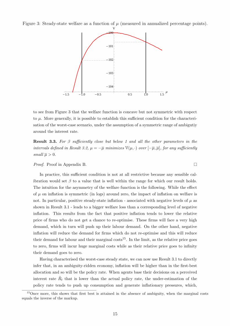
Figure 3: Steady-state welfare as a function of µ (measured in annualized percentage points).

-1.5 -1.0 -0.5 0.5 1.0 1.5Μ

-104

-103

-102

-101

-100V

to see from Figure 3 that the welfare function is concave but not symmetric with respect

to µ. More generally, it is possible to establish this sufficient condition for the characteri-

sation of the worst-case scenario, under the assumption of a symmetric range of ambigutiy

around the interest rate.

Result 3.3. For β sufficiently close but below 1 and all the other parameters in the

intervals defined in Result 3.2, µ = −µ minimizes V(µ, ·) over [−µ, µ], for any sufficiently

small µ > 0.

Proof. Proof in Appendix B.

In practice, this sufficient condition is not at all restrictive because any sensible cal-

ibration would set β to a value that is well within the range for which our result holds.

The intuition for the asymmetry of the welfare function is the following. While the effect

of µ on inflation is symmetric (in logs) around zero, the impact of inflation on welfare is

not. In particular, positive steady-state inflation - associated with negative levels of µ as

shown in Result 3.1 - leads to a bigger welfare loss than a corresponding level of negative

inflation. This results from the fact that positive inflation tends to lower the relative

price of firms who do not get a chance to re-optimise. These firms will face a very high

demand, which in turn will push up their labour demand. On the other hand, negative

inflation will reduce the demand for firms which do not re-optimise and this will reduce

their demand for labour and their marginal costs15. In the limit, as the relative price goes

to zero, firms will incur huge marginal costs while as their relative price goes to infinity

their demand goes to zero.

Having characterised the worst-case steady state, we can now use Result 3.1 to directly

infer that, in an ambiguity-ridden economy, inflation will be higher than in the first-best

allocation and so will be the policy rate. When agents base their decisions on a perceived

interest rate Rt that is lower than the actual policy rate, the under-estimation of the

policy rate tends to push up consumption and generate inflationary pressures, which,

15Once more, this shows that first best is attained in the absence of ambiguity, when the marginal costsequals the inverse of the markup.

15

in turn, lead to an increase in the policy rate. In particular, so long as φ > 1, the

policy rate will increase more than one-for-one with inflation, hence not only the actual

but also the perceived rate will be higher than its first-best value, in nominal terms.

In sum, because the policy rate responds to the endogenously determined inflation rate,

distortions in expectations have a feedback effect via their impact on the steady state level

of inflation. The combined effects of higher inflation, higher policy rates and negative µ

make the perceived real rate of interest equal to 1β , which is necessary to deliver a constant

consumption stream, i.e. a steady state. The level of this constant consumption stream

(and ultimately welfare) depends, in turn, on the price dispersion generated by the level of

inflation that characterises the steady state. The following Result summarises Results 3.1

and 3.3 and establishes more formally the effects of ambiguity on the worst-case steady

state levels of inflation and the policy rate.

Result 3.4. For β sufficiently close but below one and all the other parameters in the

intervals defined in Result 3.2, for any small enough µ > 0:

Vw(µ′) > Vw(µ) Πw(µ′) < Πw(µ) Rw(µ′) < Rw(µ) ∀ 0 ≤ µ′ < µ (16)

where the w subscript refers to welfare-minimizing steady state value of each variable over

the interval [−µ, µ].

Proof. Proof in Appendix B.

3.3 Optimal Monetary Policy

So far, we have assumed that policymakers follow a rule that would be optimal in the

absence of ambiguity (equation (7)). We now put ourselves in the shoes of a policymaker

that, having followed that rule for a long time, realizes that inflation persistently deviates

from its target and output from its potential. Our setting, however, does not readily

lend itself to a standard application of Ramsey monetary policy. The reason lies in the

fact that if a benevolent planner was to choose the interest rate, they would never select

that which minimizes welfare. Not only that, in this class of models the Euler equation

is not a binding constraint in the formulation of the Ramsey problem (see Yun, 2005).

Another way of seeing this is the following. From a timeless perspective the steady state

of the Ramsey problem corresponds, in this environment, to one in which there is no

inflation, no price dispersion and nor welfare loss of sorts. This is not surprising because

we even know a straightforward implementation of this equilibrium, which corresponds

to our model when φ → ∞. We know this is a limit case, one that is not particularly

interesting in practice so we will try to characterize optimal policy when φ is constrained

by some finite value φ.

Optimal Policy Rule. Our main optimal monetary policy result characterizes the

optimal monetary policy rule when there is a bound on the responsiveness of the policy

rate to inflation. In their analysis, Schmitt-Grohe and Uribe (2007) discuss how values

16

of φ above around 3 are unrealistic and, in practice, it is hard to appeal to values much

larger than that in light of the ZLB or just common wisdom.

Before turning to the result, it is necessary to point out that we distinguish static and

dynamic optimality, the former referring to steady states and the latter to the stabilization

of the economy around it, which we assess based on a welfare function approximation along

the lines of that in Coibion, Gorodnichenko and Wieland (2012)16

Proposition 3.1. Given the economy described in Section 3.1, a small µ > 0 and re-

stricting φ (−µ, ·) < φ ≤ φ, the following rule is statically and dynamically optimal in its

class:

Rt = R∗tΠφt (17)

where

R∗t = Rnt eδ∗(µ,φ,·) (18)

and

0 < δ∗(µ, φ; ·) < µ (19)

is implicitly defined by V(−µ+ δ∗(µ, φ; ·), ·

)= V

(µ+ δ∗(µ, φ; ·), ·

).

Proof. See Appendix C.6

We can summarize the result by saying that the central bank needs to be more hawkish

because it will respond as strongly as it possibly can to inflation and will increase the

Taylor rule’s intercept. The fact that setting φ = φ is optimal should not be surprising

at this point17. A common theme of our analysis is that the higher φ the better the

outcome in this setting, so the fact that policymakers will set its value as high as they

can is natural. The fact that the optimal intercept is higher than the natural rate would

warrant is somewhat more novel but quite intuitive too. The central bank would like to

tighten more if it had no bound on φ, because inflation is still inefficiently high. The

only other way it can do so, in this setting, is by increasing the intercept of its Taylor

rule. In doing so it runs a risk though. If it increases the intercept too much the worst

case will switch. In particular, consider a naıve policymaker who realizes the private

sector is systematically underestimating its policy rate by µ. Its response could amount

to systematically setting rates higher than its standard Taylor rule would predict by the

same amount µ. If these were just parameters and there was no minimization involved,

this policy action would implement first best18. This would be naıve because, so long as

there is some ambiguity lingering the first-best outcome will never be attained. Or, in

16The log-linear representation of the model can be found in the Appendix. For the purposes of our resultsthe crucial thing to note is that the only shock is a technology shock.

17Note that lower bound φ (−µ, ·) is simply meant to capture the lowest degree of responsiveness to inflationthat ensures determinacy for a given degree of steady-state ambiguity.

18That is because, in this economy, steady-state inflation is Π(−µ, δ(·), ·) = e−−µ+δ(·)φ−1 , so by setting δ = µ,

steady state inflation would be zero.

17

other words, if δ = µ the worst-case would no longer correspond to one in which the policy

rate is under-estimated and positive inflation creeps up in steady state. Rather it would

correspond to a situation in which the policy rate is over-estimated and deflation emerges.

At this point it is obvious that the central bank can do better than setting δ = 0 because

a small positive δ would decrease steady state inflation. At the same time setting δ = µ

is counterproductive. The optimal solution is the one in which the highest δ not causing

the worst-case to switch sides is selected (which is the equality implicitly pinning down its

value). This, in turn, highlights the fact that the policymaker is not simply facing some

kind of a constant wedge, but rather it faces a distortion that can potentially respond to

its policy-design efforts.

Another aspect of Proposition 3.1 is that the rule in equation (17) is optimal in its

class, by which we mean rules including inflation and a measure of the natural rate. One

could legitimately argue what would happen if a measure of the output gap or some other

variable was included in the specification. Rather than trying to exhaust any possible

combination we present the following corollary of Proposition 3.1 which basically states

that there cannot be a rule which outperforms the one we proposed provided we are

prepared to relax the constraint on φ. Or, equivalently, our functional form is only

(potentially) restrictive in terms of practical implementability but is otherwise as good as

any other could be.

Corollary 3.1. Given any constrained-optimal monetary policy plan, a monetary pol-

icy rule with the same functional form as that in Proposition 3.1 can be made welfare

equivalent for a suitably high level of φ.

Proof. See appendix C.7

Having demonstrated how our functional form is actually not really restrictive, one

more issue needs to be addressed: what happens if there are tradeoff-inducing shocks

on top of the TFP shock. Discussion of dynamic optimality would require a numerical

exercise, but we can definitely draw some general conclusions about the efficiency of the

steady state. In particular, as trend inflation approaches its first-best value, not only the

steady state loss is reduced but also the dynamic tradeoff between inflation and output-

gap variability is mitigated, since the coefficient on inflation variability in equation (57)

in Appendix C.5 is decreasing in trend inflation while that on output gap variability is

constant. So, for a given level of confidence µ, we might end up in the paradoxical situation

in which increasing φ all the way up to φ, might result in a reduction of the tradeoff large

enough to warrant a smaller φ from a dynamic optimality perspective. At the same time,

the coefficient on inflation in equation (57) tends to be an order of magnitude larger than

that on the output gap for the calibrations one could reasonably try, so it would appear

that setting φ = φ is the optimal thing to do under any circumstance, which is also in line

with thourough numerical experiment carried out in Schmitt-Grohe and Uribe (2007).

During the transition, our proposed rule would be sub-optimal as Yun (2005) demon-

strates. That is because our rule would implement a zero-inflation (in deviation from

target) equilibrium which is sub-optimal when starting from ∆t−1 > 1, i.e. there is some

lingering price dispersion as a legacy from the period before ambiguity was permanently

18

reduced to zero. As Yun (2005) illustrates, under those circumstances, some deflation (or

inflation below target) would be beneficial because it would reduce the price-dispersion

inefficiency at a faster pace than a zero-inflation equilibrium. In the limit, however, as

price dispersion wanes, our proposed rule would be once more optimal. Which shows how,

despite its simplicity, the specification of the policy rule we adopt is extremely robust in

this class of economies.

4 Model Validation

We take our model to the data, and show that it can, with a very standard calibration

and using the dispersion in the individual SPF nowcasts of the 3-month T-Bill rate as a

measure of ambiguity about monetary policy, explain the following stylized facts.

i. The observed decline in trend inflation over the 80s and 90s.

ii. The low, and possibly below-target, trend inflation of the last few years.

iii. The shift from equilibrium indeterminacy to determinacy in the early 1980s

iv. Paul Volcker’s apparent excessive tightening in 1982.

Ambiguity and Trend Inflation. Our headline measure of ambiguity about the

conduct of monetary policy is the interdecile dispersion of nowcasts on the 3-month TBill

rate from the Survey of Professional Forecasters, which is available from 1981Q3 onwards.

Dispersion is a standard proxy for ambiguity, and we build on the association established

above between transparency and forecast dispersion (Swanson, 2006). Finally, an impor-

tant advantage of the measure we use is that it is measured in basis points, as opposed to

being an index, hence it is more readily comparable with measures of inflation.

Figure 2 shows the 4-quarter moving-average of our preferred measure of ambiguity.

It is obvious that the degree of dispersion was an order of magnitude larger in the early

1980s than it is now. Another important fact is that, while the degree of dispersion more

than halves by the mid 80s, it still clearly trends downward through the mid 90s and

then, to a first approximation, flattens out. It is interesting to notice that it flattens

somewhere between 25 and 50bps, which means that the usual disagreement among the

hawkish and dovish ends of the professional forecasters pool amounts to situations like

the former expecting a 25bp tightening and the latter no change or 25bp loosening, a

very reasonable scenario in the late 1990s and early 2000s. In the early 80s, however,

that number was some 4-5 times larger. As large as that number can seem from today’s

vantage point, the swift monetary policy interventions that occurred in the early 80s (see

Goodfriend, 2003) can justify these levels.

Our model implies the following relationship between trend inflation and ambiguity,

which is simply the log-linear representation of equation (14) when the ambiguity interval

is symmetric (as shown in Result 3.1).

πt = π∗t +µt

φ− 1(20)

19

Figure 4: Test for the Null that individual SPF nowcasts are symmetric.

Q1−90 Q1−00 Q1−10

−3

−2

−1

0

1

2

3

4

5

H0: distribution is symmetric

skewness statisticalpha =1%alpha =5%

We test for the symmetry of the distribution of the individual SPF nowcasts of the 3-months ahead T-Bill rate.We use D’Agostino (1970) test (in red) and perform it period per period from 1981 to 2014.

This very stark relation implied by our model can be brought to the data in a very simple

way. We only need to calibrate φ, which we set to 1.5, and the target which we set to

2 percent, as indicated in Table 2. We then use the SPF interdecile dispersion measure

described above to calibrate µt. When the dispersion is roughly symmetric, it makes

sense to set µt to half the measured dispersion. To verify this assumption, we tested for

the symmetry in the dispersion of short-term rate nowcasts using a test developed by

D’Agostino (1970). Figure 4 shows that it is remarkably hard to reject symmetry up to

the point when rates approached the lower bound. At that point, as one would expect,

dispersion started to display a noticeable upward skew, as the zero lower bound provides

a natural limit to the extent that agents can forecast low rates.

We can draw a first implication from our model, simply based on this observed change

in the features of the dispersion series. That is because, under symmetry, our model

predicts trend inflation to exceed target, while in the presence of sufficiently high positive

skew the worst-case scenario switches to being one in which inflation is below target.

This is consistent with the idea that, in the past, high inflation was the policymakers’

and the public’s main concern, while in the last few years the main concern has been low

inflation instead. And it is also consistent with the decline in the inflation trend. A more

Table 2: Parameter Valuesβ Subjective Discount .995ψ Inverse Frish Elasticity 1φ Inflation Responsiveness 1.5ε Demand elasticity 15θ Calvo probability .83

20

Figure 5: Trend inflation implied by our measure of forecasters’ disagreement

82 84 86 88 90 92 94 96 98 00 02 04 06 08 10 12 14−1

0

1

2

3

4

5

6

7

8

Year

Ann

ualiz

ed P

erce

ntag

e P

oint

s

InflationVAR−based estimate of trend inflationModel−based estimate of trend inflation

Level of annualized trend inflation implied by our measure of forecasters’ disagreement in red, assuming φ = 1.5and π∗ = 2pc. The thick black line is the measure of trend inflation from the time-varying-parameters VAR,will the dotted lines are is 68% confidence bands.

accurate assessment can be obtained by plugging our measure of ambiguity in equation.

(20) and comparing the resulting measure of trend inflation with our estimates where, as

the distribution becomes asymmetric, the sign will switch.

Figure 5 overlays the measure of trend inflation implied by our model to the baseline

estimate for the trend (based on Cogley and Sbordone, 2008). The ambiguity-based

estimate of trend inflation captures the decline in the secular component of inflation in

the data. We find this very encouraging, considering this only depends on the calibration

of two parameters, which we set to standard values.

Ambiguity and Equilibrium Determinacy. It is well known that the Taylor

principle, which postulates that nominal rates should move more than one for one with

inflation, ensures equilibrium determinacy in New-Keynesian DSGE models log-linearized

around the zero-inflation steady-state (Gali’ 2008). The well known policy mistakes view

(exemplified by the work of Clarida, Galı and Gertler, 2000), attributes the high and

out-of-control inflation of the 1970s to the policy response to inflation failing to meet

the Taylor principle. Ascari and Ropele (2009), however, show that, when the model is

approximated around positive trend inflation, the Taylor principle is not a guarantee for

equilibrium determinacy. Coibion and Gorodnichenko (2011) further explore this aspect

and find that the Fed was, in all likelihood, already satisfying the Taylor principle prior

to the appointment of Chairman Volcker. They attribute the switch from indeterminate

to determinate equilibria to a fall in trend inflation. We push this argument one step

21

Figure 6: Indeterminacy region (in gray) as a function of the degree of ambiguity expressedin annualized basis points (on the horizontal axis) and the responsiveness of the policy rate toinflation (on the vertical axis). The solid black line corresponds to φ = 1.5 while the blackdashed line represents the (µ, φ) pairs consistent with annualized inflation 1.5 percent abovetarget.

Indeterminacy Region

0 50 100 150 2001.0

1.2

1.4

1.6

1.8

2.0

further. That is because trend inflation, in our model, depends, in turn, on φ, the inflation

responsiveness coefficient. In our setup, higher φ’s – typically associated with satisfying

the Taylor principle – also cause trend inflation to fall. Mechanically, a higher φ will have

the usual, direct, effect on the eigenvalues of the dynamic system, associated with the idea

that if φ > 1 real rates move in the same direction as nominal rates, thus stabilizing the

economy via their effect on consumption. Moreover, φ will affect the so called transmission

mechanism because, as shown in Appendix C the parameters of the log-linearized model

depend the level of the inflation trend, and therefore on φ. This supplementary channel

generates a non-trivial relationship between the value of φ and equilibrium determinacy

and provides another way to validate our model.

Figure 6 illustrates the determinacy region (white area) as a function of the degree of

ambiguity and φ. The black solid line in Figure 6 marks the φ = 1.5 level. Our reading of

the early 1980s is one in which φ is constant but µ falls, i.e. we are moving leftward on

the chart. We calibrate the remaining parameters of our model so that the equilibrium

switches to being determinate when the degree of ambiguity falls below 150bps, a value

that prevailed in the early 80s. Interestingly, our model can deliver this scenario under a

very reasonable calibration. The two key parameters in this respect are demand elasticity

ε, set at a value which implies a markup of about 7 percent, and the probability of

not having a chance to re-optimize prices under the Calvo-pricing scheme θ. θ is set

equal to .83, implying an average price duration of 6 quarters. So, the prediction of our

model, where we endogenize the trend but we maintain a constant response to inflation,

is consistent with the Coibion and Gorodnichenko (2011) description of the transition to

a determinate equilibrium.

22

Optimal Policy Prediction. One of the main challenges to our maintained assump-

tion that the target never changed over the last 35 or so years is the overly tight policy

stance over the course of 1982, Goodfriend (2005, p. 248). In our model a similar course

of action is perfectly sensible, for a given inflation target, if one accounts for our opti-

mal policy prediction. The immediate consequence of Result 3.1 is, in fact, that in the

presence of ambiguity extra tightening is called for.

So, while a full quantitative assessment of this effect is left for future research, Chair-

man Volckers policy is in line with our simple optimal policy prediction. If anything, the

limit of our model, in its current form, is that it does not have an explicit mechanism

linking that course of action to the increase in confidence regarding the conduct of mone-

tary policy it ensued. Rather, that effect is captured via the subsequent fall in forecasters’

forecast dispersion.

Low Inflation since 2009-2010 Over recent years, inflation trend fell below the 2%

mark. This is hardly surprising given the proximity of interest rates to their lower bound.

Indeed, it is natural to expect that in a similar situation, the worst-case scenario is one

in which rates are too high, resulting in a low level of inflation.

This is true in our model as well. We have shown above that welfare falls both when

rates are expected to be too high or too low. Our main results depend on the symmetry of

the interval over which agents are ambiguous. The lower bound on interest rates, however,

poses an inherent constraint to the possibility of excessive rate cuts, thus making it natural

to think that forecast dispersion will display a degree of upward skewness. When that is

sufficiently high, it results in the worst case switching to one in which inflation is below

the target. Figure 4 illustrates the results of statistical testing of the hypothesis that the

dispersion of forecasts is symmetric. The null hypothesis that the dispersion is symmetric

is hard to reject before the Great Recession, while is starkly rejected from 2009 onwards,

when the series displays a significant upward skew. Hence the fall in trend inflation below

2 percent is consistent with the prediction of our model in the aftermath of the Great

Recession.

5 Conclusions

We develop a model that features ambiguity-averse agents and ambiguity regarding the

conduct of monetary policy, but is otherwise standard. We show that the presence of

ambiguity has far-reaching effects, also in steady state. In particular, the model can

generate trend inflation endogenously. Trend inflation has three determinants in our

model: the inflation target, the strength with which the central bank responds to deviation

from the target and the degree of private sector confidence about the monetary policy rule.

Based on a calibration of ambiguity that matches the interdecile dispersion of the SPF

nowcasts of the current quarter’s 3-monthTBill rates, our model can explain the disinfla-

tion of the 80s and 90s as resulting from an increase in the private sector’s confidence in

their understanding of monetary policy, rather than from changes in target inflation. We

can also match the fall in trend inflation since 2009-2010 as an effect of the zero lower

23

bound. The bound sets a floor to the distortion of the interest rate and makes the worst-

case scenario shift from one in which agents fear that the interest rate will be set too low,

to one in which they fear it will be set to high. Agents base their consumptions-saving

decisions on a distorted rate that is too high and will therefore end up facing low inflation.

We also confirm the finding in Coibion and Gorodnichenko (2011) that the equilibrium in

the pre-Volcker period might have been indeterminate even though the Taylor principle

was satisfied throughout, because of the presence of trend inflation. However in our model

the trend inflation itself depends on the inflation responsiveness coefficient in the central

bank’s response function. In other words, by increasing the degree to which it responds

to inflation, a central bank will not only affect the dynamics but also the steady state

level of trend inflation.

Finally, given the importance of monetary policy for the determination of trend infla-

tion, we complete the paper studying optimal monetary policy. We can prove analytically

that, irrespective of the specifics of the parametrization, the higher the degree of ambi-

guity, the more hawkish a central banker needs to be in order to achieve a comparable

degree of welfare. Also, the higher the degree of uncertainty, the higher needs to be the

weight on inflation variability in the policymaker’s welfare-based loss function. Our re-

sults also imply that if a policymaker wanted to be less hawkish, he or she should ensure

a lower level of ambiguity about monetary policy in order to achieve a comparable degree

of welfare.

24

References

[1] Ascari, G. and T. Ropele, 2007. “Optimal monetary policy under low trend inflation,”

Journal of Monetary Economics, Elsevier, vol. 54(8), 2568-2583.

[2] Ascari, G. and T. Ropele, 2009. “Trend Inflation, Taylor Principle, and Indetermi-

nacy,” Journal of Money, Credit and Banking, vol. 41(8), 1557-1584.

[3] Ascari, G. and A. Sbordone, 2014. “The Macroeconomics of Trend Inflation,” Journal

of Economic Literature, vol. 52(3), 679-739.

[4] Baker, S. R., N. Bloom, and S. J. Davis, 2015. “Measuring economic policy uncer-

tainty,” http://www.policyuncertainty.com/media/BakerBloomDavis.pdf .

[5] Benigno, P. and L. Paciello, 2014. “Monetary policy, doubts and asset prices,” Journal

of Monetary Economics, 64(2014), 85-98.

[6] Boyarchenko, N., V. Haddad, and M.C. Plosser, 2016. “The Federal Reserve and

Market Confidence.” Federal Reserve Bank of New York Staff Reports, no. 773

[7] Calvo, G. A., 1983. “Staggered prices in a utility-maximizing framework,” Journal

of Monetary Economics, Elsevier, vol. 12(3), pages 383-398, September.

[8] Clarida, R., Gali, J. and Mark Gertler, 2000. “Monetary Policy Rules and Macroeco-

nomic Stability: Evidence and Some Theory,” The Quaterly Journal of Economics,

Vol. 115, No. 1, pp.147-180.

[9] Clark, T.E. and C. Garciga, 2016. “Trecent Inflation Trends,” Economic Trends,

Federal Reserve Bank of Cleveland.

[10] Clark, T.E. and T. Nakata, 2008. ”Has the behavior of inflation and long-term in-

flation expectations changed?,” Economic Review, Federal Reserve Bank of Kansas

City, issue Q I, pages 17-50.

[11] Cogley, T. and T.J. Sargent, 2002. “Evolving Post World War II U.S. Inflation Dy-

namics.” In NBER Macroeconomics annual 2001, edited by B.S. Bernanke and K.

Rogoff, 331-338, MIT press.

[12] Cogley, T. and A.Sbordone, 2008. “Trend Inflation, Indexation, and Inflation Persis-

tence in the New Keynesian Phillips Curve.” American Economic Review, 98(5):2101-

26.

[13] Coibion, O. and Y. Gorodnichenko, 2011. “Monetary Policy, Trend Inflation, and

the Great Moderation: An Alternative Interpretation,” American Economic Review,

vol. 101(1), pp. 341-70.

[14] Coibion, O., Y. Gorodnichenko and J. Wieland, 2012. “The Optimal Inflation Rate

in New Keynesian Models: Should Central Banks Raise Their Inflation Targets in

Light of the Zero Lower Bound?,” Review of Economic Studies, Oxford University

Press, vol. 79(4), pages 1371-1406

[15] D’Agostino, R.B., 1970. “Transformation to Normality of the Null Distribution of

g1,” Biometrika, 57(3), 679-681

25

[16] Del Negro, M., M.P. Giannoni and F. Schorfheide, 2015. ”Inflation in the Great Re-

cession and New Keynesian Models,” American Economic Journal: Macroeconomics,

American Economic Association, vol. 7(1), pages 168-96, January

[17] Del Negro, M. and S. Eusepi, 2011. “Fitting observed inflation expectations,” Journal

of Economic Dynamics and Control, Elsevier, vol. 35(12), pages 2105-2131.

[18] Drechsler, I., 2013. “Uncertainty, Time-Varying Fear and Asset Prices,” Journal of

Finance, vol. 68(5), pp. 1843-1889

[19] Ehrmann, M., S. Eijffinger and M. Fratzscher, 2012. “The Role of Central Bank

Transparency for Guiding private Sector Forecasts,” Scandinavian Journal of Eco-

nomics, 114(3),1018-1052.

[20] Epstein, L.G. and M. Schneider, 2003. “Recursive multiple-priors,” Journal of Eco-

nomic Theory, Elsevier, vol. 113(1), pages 1-31.

[21] Galı, J. 2008. Monetary Policy, Inflation, and the Business Cycle: An Introduction

to the New Keynesian Framework, Princeton University Press.

[22] Gilboa, I. and D. Schmeidler, 1989. “Maxmin expected utility with non-unique prior,”

Journal of Mathematical Economics, Elsevier, vol. 18(2), pp. 141-153

[23] Hansen, L.P. and T. J. Sargent, 2007. Robustness. Princeton University Press.

[24] Ilut, C. and M. Schneider, 2014. “Ambiguous Business Cycles,” American Economic

Review, American Economic Association, Vol. 104(8), pp. 2368-99.

[25] Kreps, D.M., 1998. “Anticipated Utility and Dynamics Choice.” In Frontiers of Re-

search in Economic Theory: The Nancy L. Schwartz Memorial Lectures 1983-1997,

edited by D.P. Jacobs, E. Kalai and M.I. Kamien, 242-74. Cambridge University

Press

[26] Lindsey, D.E., 2003. A Modern History of FOMC Communication: 1975-2002, Board

of Governors of the Federal Reserve System.

[27] Schmitt-Grohe, S. and M. Uribe, 2007. “Optimal simple and implementable monetary

and fiscal rules,” Journal of Monetary Economics, Elsevier, vol. 54(6), pages 1702-

1725.

[28] Swanson, E.T., 2006. “Have Increases in Federal Reserve Transparency Improved

Private Sector Interest Rate Forecasts?,” Journal of Money Credit and Banking, vol.

38(3), pp. 791-819

[29] Taylor, J.B., 1993. “Discretion versus Policy Rules in Practice,” Carnegie-Rochester

Conference Series on Public Policy 39: 195214.

[30] Woodford, M., 2003. Interest and Prices: Foundations of a Theory of Monetary

Policy. Princeton University Press.

[31] Yun, T. 2005. “Optimal Monetary Policy with Relative Price Distortions,”American

Economic Review, American Economic Association, vol. 95(1), pages 89-109.

26

A Some Steady state results

A.0.1 Pricing

In our model firms index their prices based on the first-best inflation, which corresponds

to the inflation target and is zero in this case. Because of ambiguity, however, steady-state

inflation will not be zero and therefore there will be price dispersion in steady state:

∆(µ, ·) =(1− θ)

(1−θΠ(µ,·)ε−1

1−θ

) εε−1

1− θΠ(µ, ·)ε(21)

∆ is minimised for Π = 1 - or, equivalently, µ = 0 - and is larger than unity for any other

value of µ. As in Yun (2005), the presence of price dispersion reduces labour productivity

and ultimately welfare.

A.0.2 Hours, Consumption and Welfare

In a steady state with no real growth, steady-state hours are the following function of µ:

N(µ, ·) =

((1− θΠ(µ, ·)ε−1

)(1− βθΠ(µ, ·)ε)

(1− βθΠ(µ, ·)ε−1) (1− θΠ(µ, ·)ε)

) 11+ψ

, (22)

while consumption is:

C(µ, ·) =A

∆(µ, ·)N(µ, ·) (23)

Hence the steady state welfare function takes a very simple form:

V(µ, ·) =1

1− β

(log (C(µ, ·))− N(µ, ·)1+ψ

1 + ψ

). (24)

Finally note that equation (22) delivers the upper bound on steady-state inflation that is

commonly found in this class of models (e.g. Ascari and Sbordone (2014)). As inflation

grows, the denominator goes to zero faster than the numerator, so it has to be that

Π (µ, ·) < θ−1ε for steady state hours to be finite19. Given our formula for steady-state

inflation, we can then derive the following restriction on the range of values µ can take

on, given our parameters:

µ >φ− 1

εlog (θ) , (25)

where the right-hand side is negative since ε > 1, φ > 1 and 0 < θ < 1. To put things

in perspective, note that the calibration in Table 2 delivers a bound of the order of −3.1

percent, which is about twice as large as the largest value suggested by our measure of

expectations disagreement. So our calibration is unaffected by this bound.

19Indeed, the same condition could be derived from the formula for price dispersion in equation (21).

27

Figure 7: Welfare function for φ = 1.5 (solid red line) and φ = 1.4 (orange dashed line).

-1.0 -0.5 0.5 1.0Μ

-103.0

-102.5

-102.0

-101.5

-101.0

-100.5

-100.0V

A.1 The role of the inflation response coefficient φ

In a model in which the only shock is a technology shock, without ambiguity any inflation

response coefficient φ larger than one would deliver the first-best allocation (see Galı,

2008), both in steady state and even period by period. As a result, from a welfare

perspective any value of φ > 1 would be equivalent. Once ambiguity enters the picture,

however, things change and the responsiveness of the Central Bank to inflation interacts

with ambiguity in an economically interesting way. In particular, it is possible to view

a reduction in ambiguity and the responsiveness to inflation as substitutes in terms of

welfare, which can be formalized as follows.

Result A.1. While parameter values are in the intervals defined in Result 3.2 and µ is

a small positive number, given any pair (µ, φ) ∈ [−µ, 0) × (1,∞), for any µ′ ∈ [−µ, 0)

there exists φ′ ∈ (1, ∞) such that:

V(µ, φ′) = V(µ′, φ)

And φ′ ≥ φ iff µ′ ≥ µ.

A corresponding equivalence holds for µ ∈ (0, µ].

Proof. Proof in Appendix B.

The intuition behind this relationship between responsiveness to inflation and ambi-

guity is the following. What ultimately matters for welfare is the steady-state level of

inflation: if ambiguity is taken as given, the only way of getting close to first-best in-

flation is for the Central Bank to respond much more strongly to deviations of inflation

from its first-best level. A higher value of φ works as an insurance that the response to

inflation will be aggressive, which acts against the effect of ambiguity about policy. At the

same time, as Schmitt-Grohe and Uribe (2007) suggest, it is practically not very sensible

to consider very high values for φ, for instance because of the possibility that a modest

cost-push shock would cause the policy rate to hit the Zero Lower Bound. So a very high

value for φ is ultimately not a solution. Figure 7 illustrates Result A.1 graphically for

28

our preferred calibration. Our baseline scenario is presented in the red solid line. If φ

was lower, say equal to 1.4, the welfare function would become steeper20 (as the orange

dashed line illustrates) because, for a given degree of ambiguity, inflation would be farther

away from first best. An application of our result works as follows in this case. Consider

a degree of ambiguity of 100bp and φ = 1.5. Figure A.1 shows graphically that the same

level of welfare can be attained when φ = 1.4, but only if ambiguity is smaller (of the

order of 80bp).

B Proofs of Steady State Results

Proof of Result 3.1

In steady state, equation 6 becomes:

1 =βR (µ, ·)Π (µ, ·)

(26)

From the Taylor rule we get:

R (µ, ·) = Rn (µ, ·) Π (µ, ·)φ eµ =1

βΠ (µ, ·)φ eµ (27)

Combining the two, delivers the first part of the result.

The second follows immediately by plugging the resulting expression for inflation into the

Taylor rule.

The inequalities result by noting that φ > 1.

Proof of Result 3.2

V (µ, ·), as defined in equation 24, is continuously differentiable around zero. Direct

computation, or noting that the first-best allocation is attained in our model when µ = 0,

shows that ∂V(µ,·)∂µ = 0.

Direct computation also delivers:

∂2V (µ, ·)∂µ2

∣∣∣∣µ=0

= −θ((β − 1)2θ + ε(βθ − 1)2(1 + ψ)

)(1− β)(θ − 1)2(βθ − 1)2(φ− 1)2(1 + ψ)

(28)

All the terms are positive given the minimal theoretical restrictions we impose, hence the

second derivative is strictly negative and there are no interior minima in a neighbourhood

of zero.

Proof of Result 3.3

Direct computation shows that the third derivative evaluated at µ = 0 can be expressed

20Note that, the welfare functions attain the same maximum at µ = 0, which illustrates the fact that theexact value of φ is irrelevant in the absence of ambiguity.

29

as:

∂3V (µ, ·)∂µ3

∣∣∣∣µ=0

=ε(2ε− 1)θ(1 + θ)

(1− β)(1− θ)3(φ− 1)3+R(β) (29)

Where, given our parameter restrictions, the first term on the RHS is positive and R(β)

is a term in β such that limβ→1− R(β) = 0.

Hence, limβ→1−∂3V(µ,·)∂µ3

∣∣∣∣µ=0

= +∞.

Moreover, ∂

(∂3V(µ,·)∂µ3

∣∣∣∣µ=0

)/∂β exists, which ensures continuity of the third derivative in

β. Hence the third derivative is positive for any β sufficiently close to but below unity.

A third-order Taylor expansion around zero can be used to show that:

V (µ0, ·)− V (−µ0, ·) =∂3V (µ, ·)∂µ3

∣∣∣∣µ=0

2µ30

6+ o(µ4

0), (30)

which is positive for a generic, positive but small value µ0 thus showing that, the steady

state value function attains a lower value at −µ0 than it does at at µ0. This, combined

with the absence of internal minima (Result 3.2), delivers our result.

Proof of Result 3.4

The first inequality follows immediately, as a weak inequality, by considering that Vw(µ′)

is the minimum value of welfare on a smaller set thanVw(µ).

The strict inequality follows from the characterization of the worst case in Results 3.2

and 3.3; in particular from the fact that Vw(µ) = V (−µ, ·) and that ∂V(µ,·)∂µ

∣∣∣µ<0

> 0 in

the vicinity of µ = 0.

For what concerns inflation, given the formula in Result 3.1, φ > 1 and given that the

worst case corresponds to µ = −µ, it is immediate to verify that µφ−1 >

µ′

φ−1 .

φ > 1 also ensures that the Taylor rule is increasing in inflation more than one for one,

which delivers the last inequality.

Proof of Result A.1

Inspection reveals that µ and φ only enter steady-state welfare through the steady-state

inflation term Π(µ, ·) = eµ

1−φ . It follows immediately that, for a given µ′, φ′ = 1 + (φ−1)µµ′

implies that (µ, φ′) is welfare equivalent to (µ′, φ). (µ, µ′) ∈ [−µ, 0)× [−µ, 0) ensures that

µ′ · µ > 0 and so φ′ ∈ (1,∞) for any φ > 1. The inequalities follow immediately from the

definition of φ′ given above and the fact that both µ and µ′ have the same sign.

A similar argument would go through for (µ, µ′) ∈ (0, µ]× (0, µ].

C Model Dynamics

To study the dynamic properties of our model, we log-linearize the equlibrium conditions

around the worst-case steady state in the usual way. As explained in Ascari and Ropele

30

(2007), having price dispersion in steady state essentially results in an additional term in

the Phillips Curve. Appendix C.1 presents the log-linear approximation around a generic

steady state indexed by µ. By setting µ = −µ, we obtain the log-linear approximation to

the worst-case steady state. An important caveat is that, in so doing, we are maintaining

that the worst case scenario corresponds to −µ in all states of the economy, but will

provide sufficient conditions for this to be indeed the case in the next paragraph. Once

we have verified our conjecture about the worst-case steady state, we turn our attention

to the implications of changes in the agents’ confidence in their understanding of the

monetary policy rule on the determinacy region and we then study the effects of shocks

to ambiguity.

C.1 Log-linearized Equations and Solution

The following equations describe the dynamics of the variables of interest around a generic

steady state indexed by µ . Setting µ = −µ one obtains the log-linear approximation

around the worst-case steady state:

ct = Etct+1 − (rt − Etπt+1)

wt = ct + ψnt

πt = κ0 (µ, ·)mct + κ1 (µ, ·)EtF2t+1 + κ2 (µ, ·)Etπt+1

rt = rnt + φπt

rt = rt + µt

mct = wt − atyt = at − ∆t + nt

ct = yt

rnt = at+1 − atynt = at

∆t = Π(µ, ·)εθ∆t−1 + ε

Π(µ, ·)εθ − (1−Π(µ, ·)εθ) θ(1

Π(µ,·)

)ε−1− θ

πt

F2t = (ε− 1)βθΠ(µ, ·)ε−1Etπt+1 + βθΠ(µ, ·)ε−1EtF2t+1

31

Where we define:

κ0 (µ, ·) ≡

((1

Π(µ,·)

)ε−1− θ)

(1− βθΠ (µ, ·)ε)

θ(31)

κ1 (µ, ·) ≡ β

((1

Π (µ, ·)

)ε−1

− θ

)(Π (µ, ·)− 1) Π (µ, ·)ε−1 (32)

κ2 (µ, ·) ≡ βΠ (µ, ·)ε−1

(θ(ε− 1)(Π (µ, ·)− 1) + (1− ε+ εΠ (µ, ·))

(1

Π (µ, ·)

)ε−1)(33)

κ3 (µ, ·) ≡ Π(µ, ·)εθ (34)

κ4 (µ, ·) ≡ ε

Π(µ, ·)εθ − (1−Π(µ, ·)εθ) θ(1

Π(µ,·)

)ε−1− θ

(35)

κ5 (µ, ·) ≡ (ε− 1)βθΠ(µ, ·)ε−1 (36)

κ6 (µ, ·) ≡ βθΠ(µ, ·)ε−1 (37)

The equations above (amended for the fact that we allow µt to vary) can be summarized

in the following system of four equations:

yt = Etyt+1 − (φπt + µt − Etπt+1)

πt = κ0 (−µ, ·)(

(1 + ψ)yt + ψ∆t

)+ κ1 (−µ, ·)EtF2t+1 + κ2 (−µ, ·)Etπt+1

∆t = κ3 (−µ, ·) ∆t−1 + κ4 (−µ, ·)πtF2t = Et

(κ5 (−µ, ·)πt+1 + κ6 (−µ, ·) F2t+1

)Where yt ≡ yt − ynt = yt − at is the output gap and κ’s are defined above. Since they

depend on steady state inflation, it is important to note that they are evaluated at the

worst-case steady state µ = −µ.

It is then possible to verify that the following guesses solve the system above21:

πt = λπ∆∆t−1 + λπµµt

yt = λy∆∆t−1 + λyµµt

F2t = λF∆∆t−1 + λFµµt

When hours enter the felicity function linearly, however, the solution simplifies further

as λπ∆ = λy∆ = λF∆ = 0. As a result, simple analytic expressions for the other un-

determined coefficients can be computed, which are reported in the main body of the

text.

21The technology process at does not enter the solution of this system because rnt is included in the Taylorrule. However it is still part of the state of the economy because it has a role in determining welfare.

32

C.2 Log-Linear solution

Appendix C.1 reports the log-linear equations that govern the evolution of our economy

around the worst-case steady state. They can be summarized into four equations:

yt = Etyt+1 − (φπt + µt − Etπt+1) (38)

πt = κ0 (−µ, ·)(

(1 + ψ)yt + ψ∆t

)+ κ1 (−µ, ·)EtF2t+1 + κ2 (−µ, ·)Etπt+1 (39)

∆t = κ3 (−µ, ·) ∆t−1 + κ4 (−µ, ·)πt (40)

F2t = Et(κ5 (−µ, ·)πt+1 + κ6 (−µ, ·) F2t+1

). (41)

where yt = ct−at is the deviation of the output gap from its worst-case steady-state level,

∆t is the price dispersion, while F2t can be interpreted as the present discounted sum

of future expected inflation rates in the recursive formulation of the optimal price-setting

equation22. The κ’s are known functions of the underlying deep parameters (including the

one governing belief distortion) defined in the Appendix and µt measures the deviation of

the distortion µt from its steady state level −µ. In particular, µt > 0 implies µt > −µ. As

a result, µt cannot take on negative values since µt = 0 corresponds to the lower bound

of the interval [−µ, µ]. In fact, we will demonstrate that welfare is increasing in µt in all

states of the economy (at, ∆t−1) under mild conditions, so that we can simply plug µt = 0

into equation (38).

To verify our conjecture that the value function is increasing around−µ we will proceed

in steps:

i. We will solve for the linear policy functions as a function of the state of the economy.

At this stage we will consider µt as an exogenous variable, i.e. our policy functions

will represent the optimal decision for a given level of µt. In doing so, we maintain

the assumption that the minimizing agent will apply the same distortion to all future

expected levels of the policy rate.

In particular a solution consists of four linear policy functions mapping{at, ∆t−1, µt

}into

{yt, πt, ∆t, F2t

}. In the appendix we report the general

solution to this guess-and-verify problem, while in the main body of the text we

focus on the special case of linear utility from leisure which allows for an analytic

solution and helps build the intuition.

ii. We will then plug the linear policy functions into the non-linear value function (once

more following Ilut and Schneider, 2014).

iii. For the case in which hours enter the felicity function linearly and the technology

process distribution has bounded support, we will provide analytic sufficient con-

ditions under which our value function is increasing around µt = 0, i.e. around

µt = −µ.

iv. We will finally verify our conjecture numerically for our preferred calibration, in

which we maintain a unitary level of the Frisch elasticity.

22Indeed it corresponds to the log-linearized version of the denominator of the expression on the RHS ofequation (13).

33

C.2.1 Special Case: Linear Hours

When hours enter the felicity function linearly (ψ = 0), the policy functions simplify and

the coefficients can be computed analytically. In particular the policy functions are:

πt = − 1

φ− 1µt (42)

F2t = − κ5

(φ− 1) (1− κ6)µt (43)

yt = −κ1λF + (κ2 − 1)λπκ0

µt (44)

∆t = κ3∆t−1 −κ4

φ− 1µt (45)

Where λF = − κ5(φ−1)(1−κ6) , λπ = − 1

φ−1 and all the κ’s are evaluated at the worst-case

steady state though we do not explicitly write this out here for the sake of notation

clarity. In this case, neither at nor ∆t−1 appear in the policy functions. The first is a

well-known consequence of the natural rate being included in the Taylor rule, an effect

that carries over even to setups in which there is price dispersion in steady state. The

second results from linearity in the utility from leisure. The policy function for inflation

is particularly interesting, as it directly reflects our discussion of steady state inflation. In

the worst-case steady state, inflation is inefficiently high. For lower levels of the beliefs’

distortion (µt ≥ 0) inflation will fall, i.e. it will get close to its first-best value. And

again, the value of φ will be critical. A higher responsiveness to inflation movements will

reduce the steady state distortion and will, consequently, reduce the responsiveness of

inflation around steady state. Indeed, φ shows up at the denominator in all the policy

functions, so higher levels of φ reduce the effects on all the variables of changes in the

distortion of beliefs. F2t is a discounted sum of future expected inflation rates, hence it

moves in the same direction with inflation. The sign of the response of the output gap,

on the other hand, varies with the steady-state degree of ambiguity. For low levels of

ambiguity, inflation and the output gap move in the same direction as in the standard

case, i.e. high inflation would correspond to an inefficiently high output gap hence a fall

in inflation will correspond to a fall in yt from a positive value down towards zero. For

sufficiently high degrees of ambiguity, however, the steady-state inefficient wedge between

hours worked and output (∆ (−µ, ·)) grows faster than hours worked and so output will

end up below potential even in the face of high steady state inflation (as discussed in

Ascari and Sbordone (2014)). As a consequence, a reduction in the distortion around the

worst-case steady state will induce a reduction in the output gap in the former case and

an increase in the latter, a fact that will play a role when defining sufficient conditions.

Finally, it is important to bear in mind that, while the the solution of the model in the

four variables described above does not depend on the level of the technology process or

of price dispersion, the variables that enter the agents’ utility do:

ct = yt + at = λY µt + at (46)

nt = yt + ∆t = λY µt + ∆t = κ3∆t−1 +

(λY −

κ4

φ− 1

)µt (47)

34

So ultimately the agents’s welfare will vary with technology and price dispersion. Indeed,

the value function for the problem, using the linear policy functions, can be expressed as:

V(at, ∆t−1; µt

)= log ((1 + ct)C(−µ, ·))− (1 + nt)N (−µ, ·) + βEtV

(at+1, ∆t; µt

)(48)

simply plugging in equations (46) and (47) for ct and nt. To build intuition, consider

the linear approximation of the log function around one, log (1 + λY µt + at) ' λY µt + at,

and the fact that, for any reasonable calibration, values of hours are indeed very close to

unity23, N (−µ, ·) ' 1. This results in the value function becoming linear. If we refer to

this approximation of the welfare function with vt and substitute forward, we get:

vt ' −κ3

1− βκ3∆t−1 + Et

[ at1− βL−1

]+

κ4

(1− κ3)(φ− 1)

(1

1− β− κ3

1− βκ3

)µt

The expression above confirms our intuition that welfare is increasing in the level of

technology and in µt (i.e. a lowering of the beliefs’ distortion), while it decreases with

higher levels of the price dispersion term. This expression is trivially minimized for µt =

024 since 0 ≤ κ3 < 1 and κ4 > 0. We can interpret vt as the average effect of a change in

µt around the worst-case steady state but since vt is linear it will not inform us on whether

µt > 0 will improve welfare in all states of the economy. Fortunately, it is immediate to

note that the value function (48) can be re-written as:

V(at, ∆t−1; µt

)= u

(−→C (−µ, ·)

)+ log (1 + ct)− ntN (−µ, ·) + βEtV

(at+1, ∆t; µt

)So we can, without any approximation at this stage, define:

dV(at, ∆t−1; µt

)≡ V

(at, ∆t−1; µt

)− V (−µ, ·) (49)

that is the non-linear difference between the welfare in any state of the economy and

welfare in the worst-case steady-state, which can be expressed as:

dV(at, ∆t−1; µt

)= log (1 + ct)− ntN (−µ, ·) + βEtdV

(at+1, ∆t; µt

)dV(at, ∆t−1; µt

)= log (1 + λY µt + at)−

((λY + κ4λπ) µt + κ3∆t−1

)N (−µ, ·))(50)

+ βEtdV(at+1, ∆t; µt

)Now the technology process enters the expression nonlinearly. So, while a change in

µt will affect the utility of leisure in a way that is independent of price dispersion and

technology, its effect on the utility from consumption will depend on the level of the

technology process. In particular, imagine a situation in which λY < 0. Equations (46)

and (47) show that both consumption and hours will fall. From our analysis above, we

know that on average the increased amount of leisure will compensate for the fall in

consumption. Whether the increased amount of leisure will actually compensate for the

lower utility from consumption in a given state of the world will, however, depend on the

23For our preferred calibration we obtain 1.0025.24Remember that µt cannot go negative as described above.

35

marginal utility of consumption. In particular, when at is very low, the marginal utility

of consumption can be high to the point where µt = 0 does not minimize welfare. The

following result formalizes this intuition, providing sufficient conditions for the welfare

function to be increasing in µt around µt = −µ.

Result C.1. Consider the economy defined above with ψ = 0, 0 ≤ κ3 < 1, κ4 ≥ 0 and at

having bounded support. Given linear policy functions, the representative agent’s welfare

is increasing in µt around µt = 0 ∀ (at, ∆t−1) ∈ [a, a]× R:

i. if λY(1+a)(1−β) ≥ Ξ(−µ, ·), when λY > 0

ii. always, when λY = 0

iii. if λY(1+a)(1−β) ≥ Ξ(−µ, ·), when λY < 0

where Ξ(−µ, ·) ≡ N (−µ, ·)(λY1−β + κ4λπ

(1−κ3)

(1

1−β −κ3

1−βκ3

)).

Proof. See Appendix C.2.1

First note that the conditions on κ3 and κ4 amount to imposing stationarity in the

dynamics of price dispersion around its steady state and the fact that inflation above

steady state will result in higher price dispersion. The former is always verified if our

model is to have solution, the second is always verified so long as in steady state inflation

is above zero (which is the case in our worst case). Assuming at has bounded support is

only needed to avoid invoking certainty equivalence. More importantly, in our experience,

Ξ(−µ, ·) < 0 for any value of µ so, in reality, the only potentially binding condition is

the third. Moreover, if we take the calibration in Table 2 and simply set ψ = 0, we find

that λY is positive for any degree of ambiguity greater than 7bp, which is less than half

the lowest value our series of expectations disagreement would imply. In other words, for

any realistic calibration of µ our sufficient conditions are trivially met. Yet, to show the

robustness of the result, let us suppose ambiguity was as low as 5bp, even in that case

any a > −.73 would do. So, provided TFP could not fall below steady state by more than

about 73 percent, our sufficient condition would be met.

C.2.2 Our preferred calibration: unitary Frisch elasticity

Linearity in the disutility of working is a convenient assumption to illustrate our point

analytically, but implies an unrealistic (infinite) value for Frish elasticity. That is why our

preferred calibration assumes ψ = 1, or a unitary Frisch elasticity. Under this assumption

we can still work out the nonlinear value function given linear policy functions, exploiting

the fact that hours enter quadratically in this specification. However the term in the past

level of the price dispersion does not drop out of the policy functions and the coefficients

cannot be computed analytically. In particular, following the same steps laid out in the

previous paragraph it is easy to obtain:

dV(at, ∆t−1; µt

)= log (1 + ct)−N (−µ, ·)2

(nt +

1

2n2t

)+ βEtdV

(at+1, ∆t; µt

)To derive our sufficient conditions (see Appendix C.3 for a complete derivation) we then

compute the derivative of dV with respect to µt and then use the conjecture that ∆t = 0 at

36

all times. This amounts to saying that our sufficient conditions have been in place for ever.

Under this conjecture, it is possible to verify that under our preferred parametrization:

i. the term corresponding to Ξ in the previous derivation is negative25.

ii. the derivative is decreasing in the level of technology26

iii. the sufficient condition that the derivative is increasing around µt = 0 is then met

for any level of the state variables.

iv. this in turn validates our conjecture that both µt and ∆t never deviate from their

worst-case steady-state level.

With this, we can proceed with rest of our analysis, taking for granted that the worst-case

will correspond to the lower bound of the interval considered by agents in all states of the

world.

C.3 Non-Linear Hours: ψ = 1

When ψ = 1, hours enter our felicity function quadratically, hence we can still use a

decomposition similar to the one we used in the linear case to obtain:

dV(at, ∆t−1; µt

)= log (1 + ct)−N (−µ, ·)2

(nt +

1

2n2t

)+ βEtdV

(at+1, ∆t; µt

)(51)

The algebra becomes a bit more cumbersome, however, because the coefficients on lagged

price dispersion in the policy functions are no longer zero:

dV(at, ∆t−1; µt

)= log

(1 + λy∆∆t−1 + λyµµt + at

)− N (−µ, ·)2

((λy∆∆t−1 + λyµµt + ∆t

)+

1

2

(λy∆∆t−1 + λyµµt + ∆t

)2)

+ βEtdV(at+1, ∆t; µt

)(52)

Substituting forward:

dV(at, ∆t−1; µt

)= Et

∞∑j=0

βj log(

1 + λy∆∆t+j−1 + λyµµt + at+j

)− N (−µ, ·)2

∞∑j=0

βj((

λy∆∆t+j−1 + λyµµt + ∆t+j

)+

1

2

(λy∆∆t+j−1 + λyµµt + ∆t+j

)2)

(53)

Then note:

∆t+j = γj+1∆ ∆t−1 + κ4λπµ

j∑l=0

γl∆µt γ∆ ≡ (κ3 + κ4λπ∆) (54)

Note that:

25Zero in the limit case in which mu = 026Similar to the first of the three cases in the previous paragraph.

37

• shocks to TFP are non-inflationary in this economy and hours do not respond

to at at all.

• hours only depend on µt, which is a choice variable for the purpose of this exer-

cise, hence there is no uncertainty involved. Intuitively, after the minimization

step is carried out, the path for hours in the foreseeable future is known without

uncertainty, because the only source of randomness (the productivity shock)

will not affect the level of hours worked in the future.

In this economy, TFP shocks do not generate inflation. If, on top of that, µt = 0 in

every period, ∆t−1 = 0 at all times. So we conjecture that ∆t−1 = 0, which amounts

to assuming that the conditions that make µt = 0 have been holding for ever and

then work out the sufficient conditions that guarantee that to be the case. Using

our conjecture:

∆t+j = κ4λπµ1− γj+1

∆

1− γ∆

µt (55)

So now we can take the derivative of dV w.r.t. µt:

∂(dV(at, ∆t−1

))∂µt

=∞∑j=0

βj

λy∆κ4λπµ1−γj

∆1−γ∆

+ λyµ(1 + λy∆∆t+j−1 + λyµµt + at+j

)− N (−µ, ·)2

∞∑j=0

βj

((λy∆κ4λπµ

1− γj∆1− γ∆

+ λyµ + κ4λπµ1− γj+1

∆

1− γ∆

)(1 + λy∆∆t+j−1 + λyµµt + ∆t+j

))

If we now evaluate the derivative at µt = 0 and ∆t = 0 at all times we get:

∂(dV(at, ∆t−1

))∂µt

∣∣∣∣∣µt=0,∆t−1=0

= Et∞∑j=0

βjλy∆κ4λπµ

1−γj∆1−γ∆

+ λyµ

(1 + at+j)

− N (−µ, ·)2∞∑j=0

βj

(λy∆κ4λπµ

1− γj∆1− γ∆

+ λyµ + κ4λπµ1− γj+1

∆

1− γ∆

)

Or:

∂(dV(at, ∆t−1

))∂µt

∣∣∣∣∣µt=0,∆t−1=0

= Et∞∑j=0

βjλy∆κ4λπµ

1−γj∆1−γ∆

+ λyµ

(1 + at+j)− N (−µ, ·)2

κ4λπµ(1− β)(1− γ∆)

(1 + λy∆ + λyµ)

+N (−µ, ·)2

κ4λπµ(1− βγ∆)(1− γ∆)

(λy∆ + γ∆)

= Et∞∑j=0

βjλy∆κ4λπµ

1−γj∆1−γ∆

+ λyµ

(1 + at+j)− Ξ (−µ, ·) (56)

Where Ξ (−µ, ·) ≡ N(−µ,·)2κ4λπµ(1−β)(1−γ∆)

(1 + λy∆ + λyµ)− N(−µ,·)2κ4λπµ(1−βγ∆)(1−γ∆)

(λy∆ + γ∆).

As before, the marginal-disutility-from-labor block is just a number, the only source

of uncertainty pertaining to the marginal utility of consumption. Again we can

exploit the fact that, on a period-by-period basis, the marginal utility is monotonic

in the level of technology, to compute sufficient conditions in the form of bounds

38

on the expected value. Clearly, we now have to rely on the numerical values of λ’s.

As it turns out, for our preferred calibration (µ = 50bp), Ξ (−µ, ·) < 0. The term

governing the marginal utility of consumption is more complicated now because of

the presence of the γj∆ term. Numerically it possible to verify that the individual

coefficients in the sum are positive. Hence the sum is minimized at a27, but even

then it would correspond to positive number. In other words our sufficient condition

is met for any value of the states.

C.4 Linear Approximation to the Welfare Function

The case in which utility is linear in hours lends itself to a very convenient approx-

imation of the welfare function so this is the avenue we pursue, but it is easy to

verify numerically that these results are robust to different values of ψ. When ψ = 0

our one-period felicity can be approximated as:

ut = log

((1 + at)A(1 + nt)N(−µ, ·)

(1 + ∆t)∆(−µ, ·)

)− (1 + nt)N(−µ, ·)

' Const+ (1−N(−µ, ·))nt − ∆t + at

' Const+ (1−N(−µ, ·))(

∆t + ct − at)− ∆t + at

' Const−N(−µ, ·)∆t +N(−µ, ·)at + (1−N(−µ, ·)) ct

We know that N(−µ, ·) ' 128 so variations in the effects of changes in µt can be

safely approximated by −∆t. Since the steady state value of ∆ is also very close

to one for the sake of this analysis we will use log differences and level differences

interchangeably and obtain:

vt ' −∆t + at + βEtvt+1

Using the law of motion ∆t and πt delivers the result in the main body of the text.

C.5 A policy-independent loss function

A quadratic approximation to the policymaker’s loss function in the tradition of

Woodford (2003) will serve us well for this purpose, because it is independent of

policy and, as such, allows us not only to pin down optimal policy but also to

rank suboptimal alternatives. Specifically, we follow Coibion, Gorodnichenko and

Wieland (2012) who derive an approximation suitable for an environment featuring

27We are obviously ruling out values of a < −1 because they would imply negative TFP in levels.28It equals 1 when µ = 0 and it takes on values of the order of 1.01 or smaller for reasonable degrees of

ambiguity, given our calibration (it equals 1.00054 for our baseline calibration).

39

trend inflation and obtain the following:

Lt =∞∑j=0

βj (Θ0 + Θ1var(yt) + Θ2var(πt)) (57)

One key difference, relative to the standard case is that a constant shows up, mea-

suring systematic loss. In fact, in our results we will discuss policy optimality along

two dimension (which mimic the discussion in Woodford (2003, p. 412)):

I. Systematic or static (or, again, average in Woodford’s words), i.e. the loss that

emerges even in steady state

II. Dynamic, the inefficiency that emerges when shocks buffet the economy

Another crucial consideration is that, as it turns out, Θ1 = 1+ψ2

is independent of

ambiguity while Θ2 is a complicated increasing function of ambiguity. This is not

really surprising since Coibion, Gorodnichenko and Wieland (2012) find that the

corresponding parameter on inflation variability is increasing in trend inflation and

we have documented above that trend inflation is a positive function of ambiguity

in our setting. It is, however, very important for our analysis, because it shows

that the lower the confidence, the more the central bank has to ”focus” on inflation,

possibly at the cost of not responding to variations in the output gap. In other

words, ambiguity exacerbates the effects of tradeoff-inducing shocks. Endowed with

a welfare-based loss function, we can now turn to characterizing optimal policy,

which we do in the next paragraph.

C.6 Proof of Proposition 3.1

The only purpose of the lower bound φ (−µ, ·) ≥ 1 is to ensure equilibrium deter-

minacy. It is not otherwise relevant as it will always be optimal to have as high a

φ as possible. Computing the steady state of the model, it is easy to verify that:

Π (µ, δ (·) , ·) = e−µ+δ(·)φ−1 (58)

while all the other steady-state expressions, as a function of inflation, remain un-

changed. Hence, if the denote with Vδ the value function of the economy in which

δ enters the Taylor rule we get that:

Vδ(µ, ·) = V(µ+ δ(·), ·) (59)

Graphically, this amounts to shifting the function leftward by δ. So Vδ inherits all

the properties of V established in Results 3.2 and 3.3, except Vδ is maximized at

−δ, the value of µ delivering zero steady state inflation. Having established this,

the proof of static optimality proceeds in three steps by first assuming a range for

δ and verifying the optimal value of φ over that range, then verifying that for the

40

optimal value of φ the optimal value of δ is pinned down by the equality in our

proposition and, finally, by establishing that the optimal value of δ indeed falls in

the range we assumed in the first part of our proof.

i. φ is the welfare-maximizing value of φ ∈ [φ, φ] ∀ µ > δ > 0.

Following the same logic as in Result A.1, it is easy to verify that for1 < φ′ < φ,

there exists a µ′ s.t.:

V (µ′, φ′, ·) = V(−µ, φ, ·

)(60)

In particular:

µ′ = −µφ′ − 1

φ− 1− δφ− φ

′

φ− 1(61)

Our restriction on δ implies that ∂µ′

∂φ′= −µ+δ

φ−1< 0. Since φ′ ∈ (1, φ)29 we know

that 0 > −δ > µ′ > −µ. Strict concavity (Result 3.2) and the fact that the

maximum is attained at −δ then imply:

V(−µ, φ, ·

)= V (µ′, φ′, ·) > V (−µ, φ′, ·) (62)

ii. δ∗(µ, φ; ·) defined by V(−µ+ δ∗(µ, φ; ·), ·

)= V

(µ+ δ∗(µ, φ; ·), ·

)is welfare

maximizing for φ = φ.

The following lemma characterizes the optimal level of δ under very general

conditions.

Lemma C.1. Assuming that V(µ, ·) takes only real values over some interval

(−m,m), is continuous, strictly concave and attains a finite maximum at µ =

µ0 ∈ (−m,m); if φ is fixed and µ > 0, then the optimal level of δ is pinned

down by the following condition.

δ∗(µ) : V (−µ+ δ∗(µ), ·) = V (µ+ δ∗(µ), ·) (63)

Proof. First we define µ0 to be the value that maximizes V (µ, ·). Strict con-

cavity ensures it is unique.

A number of different cases then arise:

1. µ0 ∈ (−µ, µ): then V′(−µ, ·) > 0 > V′(µ, ·)30

a. V(−µ, ·) < V(µ, ·). Together with strict concavity this implies that

29Where we consider the lowest possible value for φ, i.e. unity30With an abuse of notation we use derivatives here but we do not need differentiability. We just need the

function to be strictly increasing and strictly decreasing for values of µ respectively smaller and larger than µ0,which is ensured by strict concavity.

41

µws = −µ. Then there exists a small enough δ > 0 such that

V(−µ, ·) < V(−µ+ δ, ·) < V(µ+ δ, ·) < V(µ, ·).

So now the worst case µ′ws = −µ+δ generates a higher level of welfare.

The worst-case welfare can be improved until the second inequality

above holds with equality. Continuity ensures such a level of δ∗ exists.

Any value of δ > δ∗ will, however, make welfare in the worst case

decrease, and the second inequality above would reverse the sign.

b. V(−µ, ·) > V(µ, ·). Together with strict concavity, this implies that

µws = µ. Then there exists a small enough δ < 0 delivering the same

as above

c. V(−µ, ·) = V(µ, ·). There is no room for improvement. Any δ 6= 0

would lower the worst-case welfare.

2. µ0 ≥ µ. Strict concavity implies that V (−µ, ·) < V (µ, ·). Hence µws =

−µ. For all 0 ≤ δ ≤ µ0 − µ

V(−µ, ·) < V(−µ+ δ, ·) < V(µ+ δ, ·) ≤ V(µ0, ·)

For δ just above µ0 − µ we fall in case 1a above.

3. µ0 ≤ −µ. Strict concavity implies that V (−µ, ·) > V (µ, ·). Hence µws =

µ. For all µ0 − µ ≤ δ ≤ 0

V(µ0, ·) ≥ V(−µ+ δ, ·) > V(µ+ δ, ·) > V(µ, ·)

For δ just above µ0 − µ we fall in case 1b above.

The conditions of the Lemma apply to our case for sufficiently small degrees

of ambiguty (as maintained in Results 3.2 and 3.3), which also ensure that

m meets the condition in equation (25), which we assume throughout. The

Lemma holds for a generic fixed φ, so it obviously applies to φ = φ.

iii. in the economy described in Section 3.1, 0 < δ∗(µ, φ; ·) < µ.

Results 3.2 and 3.3 ensure that our economy falls under case 1a of Lemma

C.1. This proves that δ∗(µ) > 0. Suppose now that δ∗(µ) ≥ µ. That would

push the argmax of the welfare function outside (or on the boundary) of [−µ, µ],

which can never be optimal given strict concavity (similar arguments to cases

2 and 3 in Lemma C.1).

42

These three points complete the proof of the static optimality of our proposed rule.

Dynamic optimality follows immediately by noting that the first-order solution to

our model (Appendix B.1) implies that both inflation and the output gap do not

vary with TFP, hence the variance of both the output gap and inflation - equation

(57) - is minimized.

C.7 Proof of Corollary 3.1

This sufficient condition can be derived even for δ = 0, so we will assume that for

expositional simplicity. Setting δ optimally will simply make the suitably high level

of φ somewhat lower.

Consider any policy plan delivering utility v0 in steady state. Suppose that is

welfare-superior to the policy currently in place V(−µ, φ, ·) < v0 ≤ V(0, φ, ·), where

the latter is the first-best allocation so it cannot be improved upon.

Results 3.2 and 3.3 ensure the value function is strictly increasing for µ < 0 so there

exists a µ′, −µ < µ′ ≤ 0, s.t. V(µ′, φ, ·) ≥ v0. Result A.1 then ensures there also

exists φ′ s.t. V(−µ, φ′, ·) = V(µ′, φ, ·). Since our proposed monetary policy rule

is also dynamically optimal for any value of φ that guarantees determinacy, any

φ ≥ φ′ allows our monetary policy to deliver at least as high a welfare level as the

alternative delivering v0.

43