UNIVERSITY OF CALIFORNIA

SANTA CRUZ

AN ADAPTIVE FRAMEWORK FOR IMAGE AND VIDEOSENSING

A thesis submitted in partial satisfaction of therequirements for the degree of

MASTER OF SCIENCE

in

ELECTRICAL ENGINEERING

by

Lior Zimet

March 2005

The Thesis of Lior Zimetis approved:

Professor Peyman Milanfar, Chair

Professor Ali Shakouri

Professor Hai Tao

Robert C. MillerVice Chancellor for Research andDean of Graduate Studies

Copyright c© by

Lior Zimet

2005

Contents

List of Figures v

Abstract vi

Dedication viii

Acknowledgements ix

1 Introduction 11.1 The Imaging Sensor Spatio-Temporal Characteristics . . . . . . . . . 11.2 Adaptive Versus Non-Adaptive Image Sensing . . . . . . . . . . . . . 31.3 Related Work . . . . . . . . . . . . . . . . . . . . . . . . . . . . . . . . 81.4 Thesis Contribution and Organization . . . . . . . . . . . . . . . . . . 9

2 Video Content Measure 102.1 Spatial Content Measure . . . . . . . . . . . . . . . . . . . . . . . . . . 11

2.1.1 Frequency Domain and Entropy Methods . . . . . . . . . . . . 112.1.2 Proposed Measure of Content . . . . . . . . . . . . . . . . . . . 152.1.3 Spatial content measure using �2-norm . . . . . . . . . . . . . . 23

2.2 Temporal content measure . . . . . . . . . . . . . . . . . . . . . . . . . 24

3 Sensor operating point 293.1 Operating point definition . . . . . . . . . . . . . . . . . . . . . . . . . 293.2 Operating point computation . . . . . . . . . . . . . . . . . . . . . . . 313.3 Projection to the sensor operating space . . . . . . . . . . . . . . . . . 33

4 Closed loop operation 374.1 Adaptive imaging control system . . . . . . . . . . . . . . . . . . . . . 374.2 Real-time open loop experiment . . . . . . . . . . . . . . . . . . . . . . 394.3 Closed loop simulation . . . . . . . . . . . . . . . . . . . . . . . . . . . 42

iii

5 Conclusions and future work 46

A Simulation environment 49

Bibliography 54

iv

List of Figures

1.1 Typical tradeoff of spatial vs. temporal sampling in imaging sensor . 31.2 Adaptive versus non-adaptive sampling . . . . . . . . . . . . . . . . . 41.3 An adaptive sensor block diagram . . . . . . . . . . . . . . . . . . . . 51.4 An adaptive sensor with three-sensor configuration block diagram . . 7

2.1 Γ(F) operator for a one dimensional signal . . . . . . . . . . . . . . . 122.2 Zoneplate images used for the evaluation of the content measure . . . 132.3 Frequency domain spatial content measure . . . . . . . . . . . . . . . . 142.4 The spatial window and the decaying factors of the �1-norm spatial

content measure . . . . . . . . . . . . . . . . . . . . . . . . . . . . . . 162.5 Histogram example of the vector Z for obtaining the content measure 172.6 �1-norm spatial content measure behavior for WGN content . . . . . . 192.7 �1-norm spatial content measure with added WGN . . . . . . . . . . . 202.8 Noisy measure bias and corresponding polynomial fits for different noise

levels . . . . . . . . . . . . . . . . . . . . . . . . . . . . . . . . . . . . . 212.9 Example of noise compensation in a natural video sequence with σ = 20 222.10 �2-norm spatial content measure behavior for WGN content . . . . . . 242.11 �2-norm spatial content measure with added WGN . . . . . . . . . . . 252.12 The temporal window and the decaying factors of the �1-norm temporal

content measure . . . . . . . . . . . . . . . . . . . . . . . . . . . . . . 262.13 �1-norm temporal content measure behavior for WGN content . . . . . 272.14 �1-norm temporal content measure with added WGN . . . . . . . . . . 282.15 Pixels value along the time axis of synthesized sequences for the evalu-

ation of the temporal content measure . . . . . . . . . . . . . . . . . . 28

3.1 Example of sensor operating space and operating point . . . . . . . . . 303.2 Spatial content measure to sampling rate conversion . . . . . . . . . . 333.3 Temporal content measure to sampling rate conversion . . . . . . . . . 343.4 Projection of operating point to sensor operating space - point is within

the space . . . . . . . . . . . . . . . . . . . . . . . . . . . . . . . . . . 35

v

3.5 Projection of operating point to sensor operating space - point is outsidethe space . . . . . . . . . . . . . . . . . . . . . . . . . . . . . . . . . . 36

4.1 Closed loop operation . . . . . . . . . . . . . . . . . . . . . . . . . . . 394.2 Video and graphic display of the IEEE1394 real-time experiment . . . 414.3 Content measure control window of the IEEE1394 real-time experiment 424.4 Operating space created for the closed loop simulation . . . . . . . . . 434.5 Spatial and temporal content measures of the football sequence . . . . 454.6 Input images from the football sequence at the operating point transi-

tions. The numbers below each picture indicate the computed operatingpoints of the closed loop operation. . . . . . . . . . . . . . . . . . . . . 45

A.1 Example of conversion graph for transport stream data to uncompressedbinary . . . . . . . . . . . . . . . . . . . . . . . . . . . . . . . . . . . . 50

A.2 Sensor operating space preparation from high definition video source . 51A.3 Block diagram of the closed loop simulation environment . . . . . . . . 53

vi

Abstract

An Adaptive Framework for Image and Video Sensing

by

Lior Zimet

Current digital imaging devices often enable the user to capture still frames at a high

spatial resolution, or a short video clip at a lower spatial resolution. With bandwidth

limitations inherent to any sensor, there is clearly a tradeoff between spatial and tem-

poral sampling rates, which present-day sensors do not exploit. The fixed sampling

rate that is normally used does not capture the scene according to its content and

artifacts such as aliasing and motion blur appear. Moreover, the available bandwidth

on the camera transmission or memory is not optimally utilized. In this paper we

outline a framework for an adaptive sensor where the spatial and temporal sampling

rates are adapted to the scene. The sensor is adjusted to capture the scene with re-

spect to its content. In the adaptation process, the spatial and temporal content of the

video sequence are measured to evaluate the required sampling rate. We propose a ro-

bust, computationally inexpensive, content measure that works in the spatio-temporal

domain as opposed to the traditional frequency domain methods. We show that the

measure is accurate and robust in the presence of noise and aliasing. The varying sam-

pling rate stream captures the scene more efficiently and with fewer artifacts such that

in a post-processing step an enhanced resolution sequence can be effectively composed

or an overall lower bandwidth can be realized, with small distortion.

To my wife Miriam Sivan-Zimet and my son Yoav

viii

Acknowledgements

I would like to express my gratitude to my advisor Prof. Peyman Milanfar

for guiding me throughout this work, supporting my ideas, and introducing me to the

world of research. His invaluable suggestions helped me to seek the right direction in

this research. I also thank my other committee members Prof. Ali Shakouri and Prof.

Hai Tao for their review and comments.

Special thanks to my colleagues at the Multi-Dimensional Signal Process-

ing (MDSP) group Sina Farsiu, Dirk Robinson, and Amyn Poonawala and especially

Morteza Shahram for fruitful discussions and collaboration.

I wish to thank my friend Tamar Kariv for her great support with software

development and advise. I also wish to thank Steven Brook, my manger at Zoran

corporation, for for his support in my studies and for the flexibility he gave me at

work in order to pursue this MS degree.

Above all, the love, care, patience, and support of my wife Miri and my son

Yoav. Nothing would have happened without them!

Santa Cruz, CA March 18, 2005 Lior Zimet

ix

Chapter 1

Introduction

In this chapter we introduce the adaptive imaging framework. We provide a brief

description of the imaging sensor spatio-temporal characteristics and show how it can

be used to capture the scene more effectively. We show possible sensor architectures

and provide the general description for an adaptive sensor operation. Finally, we list

related works and the thesis organization.

1.1 The Imaging Sensor Spatio-Temporal Characteristics

Imaging devices have limited spatial and temporal resolution. An image is

formed when light energy is integrated by an image sensor over a time interval. The

minimum energy level for the light to be detected by the sensor is determined by signal

to noise ratio characteristics of the detector [5]. Therefore, the exposure time required

to ensure detection of light is inversely proportional to the area of the pixel. In other

1

words, exposure time is proportional to spatial resolution. This is the fundamental

trade off between the spatial sampling (number of pixels) and the temporal sampling

(number of images per second). Other parameters such as readout and analog to digital

conversion time as well as sensor circuit timing have second order effects on the spatio-

temporal trade-off. Figure 1.1 is an example of the spatio-temporal sampling rate

tradeoff in a typical camera (e.g. PixeLINK PL-A661). The markers along the graph

are typical sampling rates used by digital image sensors for different applications. The

parameters of the trade-off line are determined by the characteristics of the materials

used by the detector and the light energy level. A conventional video camera has a

typical temporal sampling rate of 30 frame per second (fps) and a spatial sampling

rate of 720×480 pixels, whereas a typical still digital camera has spatial resolution of

2048×1536 pixels.

The minimal size of spatial features or objects that can be visually detected

in an image is determined by the spatial sampling rate and the camera-induced blur.

The maximal speed of dynamic events that can be observed in a video sequence is

determined by the temporal sampling rate [14]. We define the sensor operating point

as the pair of {spatial sampling rate, temporal sampling rate} at which the sensor is

operating.

2

0 50 100 150 200 250 300 3500

2

4

6

8

10

12

14x 10

5

Frame Rate [FPS]

Num

ber

of P

ixel

s

1280x1024

1024x768

800x600

640x480

320x240 64x64

Figure 1.1: Typical tradeoff of spatial vs. temporal sampling in imaging sensor

1.2 Adaptive Versus Non-Adaptive Image Sensing

A non-adaptive sensor is normally set to a fixed operating point, which does

not depend on the scene. Therefore, the data from the sensor can be spatially or

temporally aliased due to insufficient sampling rate. Insufficient temporal sampling

rate introduces motion based aliasing. Motion aliasing occurs when the trajectory

generated by a fast moving object is characterized by frequencies which are higher than

the temporal sampling rate of the sensor. In this case, the high temporal frequencies

are folded into the low temporal frequencies. The observable result is a distorted or

even false trajectory of the moving object [14] (e.g. wheels on a fast-moving cart

appearing to rotate backwards in a film captured at typical video rate). Meanwhile,

3

insufficient spatial sampling rate will remove details from the image and introduce

visual effects such as blur and aliasing.

Now, instead of relying on a single point on the spatio-temporal tradeoff

curve (Figure 1.1), we could adapt the sensor to run at an operating point that is

determined by the scene. An adaptive sensor would have the ability to change its

operating point according to a measure of the temporal and spatial content in the

scene. It therefore captures the scene more accurately and more efficiently with the

available bit-rate or sensor memory or communication capabilities. The design of such

a novel sensor can also be informed by user preferences in terms of acceptable levels

of spatial or temporal aliasing or other factors. Figure 1.2 is an illustration of the

sampling difference between an adaptive and non-adaptive imaging sensor. A Block

diagram of an adaptive sensor is shown in Figure 1.3.

Fixed Sampling

t

m x n

t1

t2

t3

Adaptive Sampling

m1 x n1

m2 x n2

m3 x n3

Figure 1.2: Adaptive versus non-adaptive sampling

The spatial and temporal dimensions are very different in nature, yet are

4

Spatial ContentMeasure

Temporal ContentMeasure

OperatingPoint

Computation

AdaptiveImagingSensor

Adaptation feedback

Figure 1.3: An adaptive sensor block diagram

inter-related through the sensors capabilities. In the proposed adaptive sensor ar-

chitecture we measure the spatial and temporal content separately to determine the

required sampling rate for the current scene. We develop a robust, computationally

inexpensive, measure for the scene content. The measure works in the spatio-temporal

domain as opposed to the traditional frequency domain. We show that the measure

is usable in the presence of noise and aliasing. Section 2 of the paper describes the

content measure along with other possible methods.

In the single sensor architecture as shown in Figure 1.3, the content mea-

sure is computed on the same data that the sensor is capturing at different operating

points. Therefore, the accuracy of the spatial and temporal content measures depends

on the operating point. Higher sampling will result in a more accurate measure and

vice versa. An optional architecture would be a three-sensor configuration as depicted

5

in Figure 1.4. Here we dedicate a high frame rate, low spatial resolution sensor for

the temporal content measure and a low frame rate high spatial resolution sensor for

the spatial content measure. The scene capture is done through a third sensor that

has variable spatio-temporal sampling capabilities. Although this architecture pro-

vides more accurate measure for the scene content it is less applicable in practice and

imposes other issues such as three-way optical beam splitting and circuit complexity.

As further described in Chapter 4, in single sensor architecture the content measure

is compromised only in the transitions between operating points and the system con-

vergence to correct operating point is guaranteed.

The adaptive sensor measures the scene content continuously for every in-

coming frame. The required sampling rate is then determined from this measure. The

required sampling rate can sometimes be out of the sensor’s capabilities and a projec-

tion to the nearest possible operating point in the sensor’s operating space is required.

The conversion from the content measure to sensor operating point is discussed in

Chapter 3. Using a feedback loop the sensor is reconfigured to the new operating

point.

Another important aspect of a sensor’s capability is the data transmission

bandwidth at its output. A fixed sampling rate of the sensor determines a fixed

bit-rate at the output assuming no compression involved. But in many cases such

as static scenes or scenes with very little details the said bandwidth is not utilized

efficiently. In the adaptive framework, the sensor determines the required sampling

rate and can therefore either reduce the bit-rate to the minimum necessary, or use

6

HighTemporalSampling

RateSensor

High Spatialsampling rate

Sensor

Spatial ContentMeasure

TemporalContentMeasure

Operating PointComputation

Feedback

AdaptiveImagingSensor

DataOutput

Figure 1.4: An adaptive sensor with three-sensor configuration block diagram

the available bandwidth to increase the spatial sampling rate at the expense of the

temporal sampling rate and vice versa.

The video sequence at the output of an adaptive sensor is a set of frames

at varying spatial and temporal sampling rates. This three dimensional data cube

represents the scene as was sampled by the sensor after adaptation. If the sensor

sampled the scene as dictated by the content measure, this cube of data, in the ideal

case, should include sufficient information to restore a high resolution spatio-temporal

7

sequence. In some cases, the sensor operating space will limit the sampling rate

and a bias towards the temporal or the spatial sampling rate has to be introduced.

In both cases of ideally sampled and under sampled scene, a restoration is possible

using methods such as space-time super-resolution [14, 8] and motion compensated

interpolation [17].

1.3 Related Work

The use of imaging sensors at different operating points is the basis of other

related work. Ben-Ezra and Nayar [2] have used a hybrid sensor configuration to

remove motion blur from still images. In their approach, one sensor works in a high

temporal, low spatial sampling rate operating point to capture the motion during

image integration time. A second sensor acquires the image in high spatial sampling

rate and uses the motion information from the first sensor to deblur the image. Lim

[12] has employed very high temporal sampling at the expense of spatial sampling to

restore a high resolution sequence. Other related work are from the voice recognition

field [22, 23]. Here, the use of variable frame rate (VFR) is applied to speech analysis.

The frame rate is determined by a content entropy measure on the recorded audio

signal.

8

1.4 Thesis Contribution and Organization

In this thesis we introduce a novel approach for video and image sensing.

We have experimentally developed a framework for an adaptive sensor that is simple

enough to be implemented as part of the sensor circuit. We explore techniques for

measuring the content in a video sequence and the correlation of the content measure

to the required sampling rate. The proposed content measure in the framework is

robust with respect to noise and aliasing and can be used in a single sensor system

configuration. A complete closed loop operation of a single sensor adaptive sensing

system has been simulated using natural scene video sequences.

The thesis is organized as follows. In Chapter 2 we explore traditional meth-

ods for video content measure and propose a measure based on the �1-norm operation.

We show the advantage of using the proposed measure in terms of behavior with noise

and complexity. In Chapter 3 we define the sensor operating point and the way to

obtain it from the content measure proposed in Chapter 2. Chapter 4 describes the

operation of the sensor as a control system. It describes a real-time open loop experi-

ment and the closed loop simulation along with their results. Chapter 5 conclude the

thesis and give insight into future work in this framework.

9

Chapter 2

Video Content Measure

The purpose of the content measure is to quantify the spatial and temporal informa-

tion in the scene. By spatial information we mean details or spatial frequency content.

Temporal content information is the change along the time axis or temporal frequency

content. Accurate measurement of the content will allow us to determine the required

sampling rate and to adjust the imaging sensor accordingly. Traditional methods use

frequency domain analysis to measure the frequency content of the image sequence. As

we show in Section 2.1.1, the frequency domain measure becomes unreliable with the

existence of noise. Entropy measures as used in the speech recognition application[23]

are computationally inexpensive but seem not to be robust in terms of accuracy for

video data content measure. Other methods [21] [15] are based on Shannon’s infor-

mation theory and provide metrics for quality assessment and visualization.

In the adaptive sensor framework,the objective is to keep the computational

requirements minimal so that simple and cost effective implementation is possible.

10

The chosen quantitative measure needs to be robust and accurate in the presence of

noise and aliasing. In this chapter we first present the frequency domain and entropy

methods for content measure and their characteristics with noise and aliasing. Noting

their shortcomings, we then suggest a content measure in the spatial domain that

is computationally inexpensive and can work robustly in the present of noise and

aliasing. The content measure is first presented for the spatial case. An extension of

the suggested measure for the temporal case is described in Section 2.2. In the rest

of the thesis we use the proposed spatial and temporal measure in the development of

the adaptive imaging framework.

2.1 Spatial Content Measure

The spatial content measure is trying to quantify the spatial information in

the scene. By spatial information we mean details or spatial frequency content. In

this section we explore the traditional frequency domain and entropy methods, we

show their shortcomings and propose a measure based on an �1-norm operation. An

alternative measure based on the �2-norm operation is briefly described at the end of

the section.

2.1.1 Frequency Domain and Entropy Methods

Measuring the spatial content in the frequency domain is naturally translated

to a two-dimensional fast Fourier transform (FFT) of the image. The image content

is determined to be at the frequency where, say, 99% of the total energy under the

spectrum is captured as depicted in Figure 2.1 for a one dimensional signal.

11

We can define:

F = FFT2D(X) (2.1)

where X is a matrix with N pixels presenting the luminance values of the image and

FFT2D(·) is a two dimensional matrix that represents the energy level of the image

in the frequency domain. The content measure finds the frequency where most of the

total energy in the FFT2D matrix has been captured. Assuming the center of the

matrix F is the DC bin and it has N elements, the content figure is the index such

that γ∑N

i=0 |F|2i has been integrated from the center pixel out. γ is a number close to

1 that determines the point where the frequency energy has significantly dropped.

0 0.5 1 1.5 2 2.5 3 3.50

1

2

3

4

5

6

|F|2

Frequency

Γ(F)

Figure 2.1: Γ(F) operator for a one dimensional signal

In the absence of noise, this measure gives an accurate figure for the content

12

in the image. However, the two-dimensional FFT operation is sensitive to noise. We

synthesized a sequence of images for the evaluation of the content measure with respect

to spatial bandwidth and noise. The sequence was composed of spatial zoneplate

images (Figure 2.2) with frequency content from DC up to a certain known value. The

sequence is composed such that the frequency bandwidth of a consecutive zoneplates in

the sequence is linearly increasing and all images were sampled above their respective

Nyquist rate. Figure 2.2 is an example of four zoneplate images from the simulation

with different frequency content.

Figure 2.2: Zoneplate images used for the evaluation of the content measure

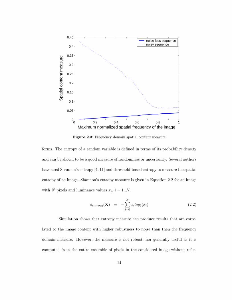
Figure 2.3 is the simulation results of the frequency domain content measure

on the synthesized sequence. The solid line is the content measure of the clean images

and it strongly corresponds to the linearly increasing bandwidth of the sequence. The

dashed line is the content measure for the same sequence with added white Gaussian

noise (WGN) with standard deviation of 20. It is clear that the noise distorts the

content measure in a non-linear way such that it does not reflect the image content

correctly and makes compensation rather difficult.

Entropy methods for determining signal properties have a wide variety of

13

0 0.2 0.4 0.6 0.8 10

0.05

0.1

0.15

0.2

0.25

0.3

0.35

0.4

0.45

Maximum normalized spatial frequency of the image

Spa

tial c

onte

nt m

easu

re

noise less sequencenoisy sequence

Figure 2.3: Frequency domain spatial content measure

forms. The entropy of a random variable is defined in terms of its probability density

and can be shown to be a good measure of randomness or uncertainty. Several authors

have used Shannon’s entropy [4, 11] and threshold-based entropy to measure the spatial

entropy of an image. Shannon’s entropy measure is given in Equation 2.2 for an image

with N pixels and luminance values xi, i = 1..N .

sentropy(X) = −N∑

i=0

xilog2(xi) (2.2)

Simulation shows that entropy measure can produce results that are corre-

lated to the image content with higher robustness to noise than then the frequency

domain measure. However, the measure is not robust, nor generally useful as it is

computed from the entire ensemble of pixels in the considered image without refer-

14

ence to the relative position of the neighboring gray values. That is, if the pixel gray

values at various (or all) positions in a given image are randomly swapped with values

at other pixel positions, the very same entropy measure still results. Therefore, it is

impossible to relate the scalar output of the measure to the actual content.

2.1.2 Proposed Measure of Content

For a natural image it has been experimentally shown that the differences

between adjacent pixel values mostly follow the Laplacian probability density law. Be-

sides we can reasonably assume that in practice these differences are independent from

each other [9]. By employing this significant observation, we suggest a methodology

to measure the spatial and temporal content. In the proposed framework, obtaining a

figure for the content in spatial and temporal domains can be translated to a window

operation using �1-norm as follows. Let X denote the (say raster scan) vectorized no-

tation of the acquired image with elements xi,j . Based on the above statistical model,

we first utilize the following nonlinear �1-based filter [7, 8] applied to each pixel in the

image:

zi,j =p∑

m=−p

p∑l=−p

α|m|+|l| |xi,j − xi−l,j−m| , (2.3)

where the weight 0 < α < 1 is applied to give a spatially decaying effect to

the summation, effectively giving bigger weight to higher frequencies. Other decaying

factors can be used such as pixel distance from the center pixel or look-up tables in

cases where lower complexity or real-time operation is required. zi,j (or in vector form

Z) is directly related to the (log-)likelihood of the image according to the assumed

15

statistical model. The window operation for p = 2 with the decaying factors is illus-

trated in Figure 2.4. The differences are taken between the center pixel and all the

neighboring pixels in the window and weighted by the corresponding decaying factor.

Figure 2.4: The spatial window and the decaying factors of the �1-norm spatial contentmeasure

To obtain a reasonably robust content measure, one can think of first finding

the histogram of Z (call the value of this histograms pk at bin k = 0, 1, · · · , M − 1)

and then finding the value of the histogram bin (l) such that

l∑k=0

pk ≥ ηM−1∑k=0

pk (2.4)

where η denotes the percentage of the total area under the curve we want to contribute

in computing the content (for example 95%). Figure 2.5 is an example for a histogram

computed on a natural image with α = 0.5 and p = 2.

16

0 0.2 0.4 0.6 0.8 1 1.2 1.4 1.6 1.8 20

1

2

3

4

5

6x 10

5

Content measure figure

Num

ber

of w

indo

ws

95% of total energy

Figure 2.5: Histogram example of the vector Z for obtaining the content measure

Since computing the histogram in real-time is computationally taxing, a rea-

sonable alternative can be employed based on the Chebyshev inequality[13],

p(|ξ − µξ| ≥ cσξ) ≤ 1c2

(2.5)

where µξ and σξ denote the mean and variance of the random variable ξ and p(·) is the

probability. From the Chebyshev inequality, we can determine the coefficient c based

on the value of η. As an example for η = 0.96, we have c = 5. Next, we compute

the mean and variance over the ensemble of elements of Z (µz and σ2z). Finally, the

content measure denoted by ρ(Z) is obtained by

ρ(Z) = µz + cσz. (2.6)

17

The proposed �1-based operation is computationally inexpensive (order of

N versus Nlog(N) in the FFT case) and proves to perform well as compared to

frequency domain and entropy measures. We characterize the spatial �1-norm measure

with respect to additive white Gaussian noise, measure correlation to the content

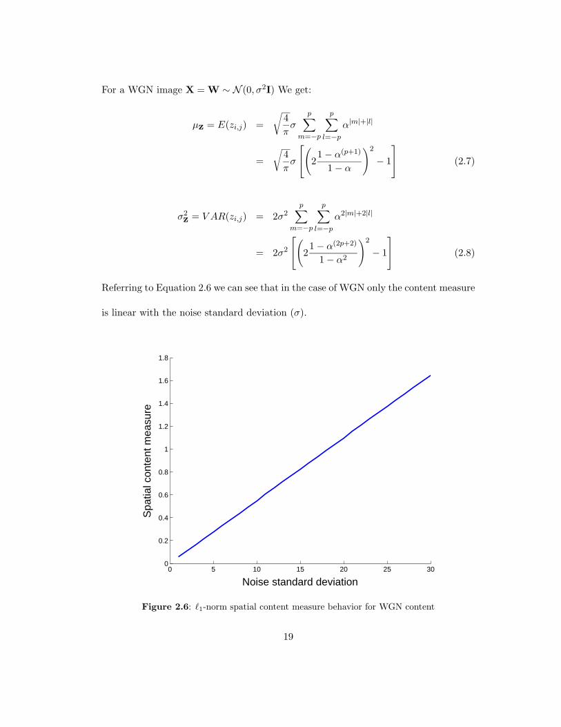
bandwidth, and analyze its behavior with the presence of aliasing. Figure 2.7 is the

simulation results of the �1-norm content measure on a synthesized sequence with a

known frequency content. The sequence is the same one synthesized for the frequency

domain measure in Section 2.1.1.

The solid line is the content measure of the synthesized sequence with no

added noise. The measure behavior is monotonically increasing and strongly corre-

lates to the linearly increasing bandwidth of the sequence. Figure 2.7 also shows the

behavior of the �1-norm measure for added WGN with different variance (σ2). As

opposed to the frequency domain measure with added noise, the behavior of the �1-

norm measure conserves the ratio of high and low content and can be compensated

for rather easily, assuming σ2 is known 1 or can be estimated [10].

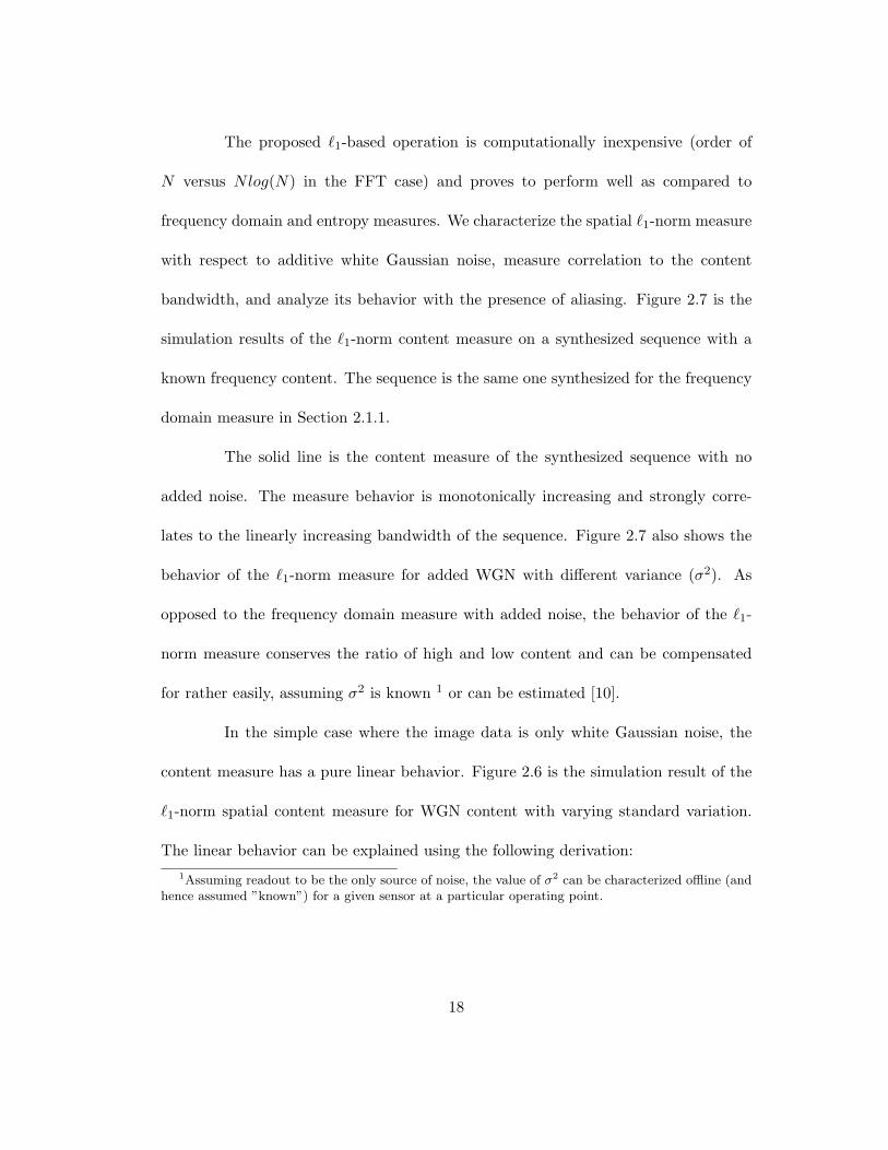
In the simple case where the image data is only white Gaussian noise, the

content measure has a pure linear behavior. Figure 2.6 is the simulation result of the

�1-norm spatial content measure for WGN content with varying standard variation.

The linear behavior can be explained using the following derivation:1Assuming readout to be the only source of noise, the value of σ2 can be characterized offline (and

hence assumed ”known”) for a given sensor at a particular operating point.

18

For a WGN image X = W ∼ N (0, σ2I) We get:

µz = E(zi,j) =√

4π

σp∑

m=−p

p∑l=−p

α|m|+|l|

=√

4π

σ

⎡⎣

(21 − α(p+1)

1 − α

)2

− 1

⎤⎦ (2.7)

σ2z = V AR(zi,j) = 2σ2

p∑m=−p

p∑l=−p

α2|m|+2|l|

= 2σ2

⎡⎣

(21 − α(2p+2)

1 − α2

)2

− 1

⎤⎦ (2.8)

Referring to Equation 2.6 we can see that in the case of WGN only the content measure

is linear with the noise standard deviation (σ).

0 5 10 15 20 25 300

0.2

0.4

0.6

0.8

1

1.2

1.4

1.6

1.8

Noise standard deviation

Spa

tial c

onte

nt m

easu

re

Figure 2.6: �1-norm spatial content measure behavior for WGN content

19

In natural scenes, the xi,j in Equation 2.10 are not independent values. Since

the �1-norm is not a linear operation, a simple analytical derivation for the behavior of

the measure is rather difficult to find. As shown in Figure 2.7, additive noise creates

a non-linear behavior to the content measure that can be modelled and compensated

for.

0 0.1 0.2 0.3 0.4 0.5 0.6 0.7 0.8 0.9 10

0.5

1

1.5

2

2.5

3

Normalized spatial frequency

Spa

tial C

onte

nt E

stim

atio

n

σ=10σ=15σ=20σ=25σ=30 .

No added noise

Figure 2.7: �1-norm spatial content measure with added WGN

Using large data base of training data, the compensation is done by char-

acterizing the bias between the noisy measure and the pure measure for the range

of possible noise levels. This characterization leads to a 4th order polynomial that

provide the bias level with respect to the noise standard deviation (σ). The general

behavior as shown in Figure 2.7 is that content that produce low content measure will

20

suffer from larger bias and the bias is approximately constant as the content figure

exceed a certain level. Figure 2.8 provides the bias behavior along with its polynomial

fit for noisy measures with σ = 10, σ = 20, and σ = 30. Equation 2.9 is an exam-

ple for a polynomial fit of the noise bias with respect to the content measure (ρ) for

σ = 20. The polynomial coefficients can be tabulated with respect to σ for different

noise levels.

Content Measurement Bias(σ=20) =

3 ∗ 10−9ρ4 − 2.8 ∗ 10−6ρ3 + 0.00059ρ2 − 0.041ρ + 1.1 (2.9)

0 0.2 0.4 0.6 0.8 10

0.2

0.4

0.6

0.8

1

1.2

1.4

1.6

1.8

Normalized spatial frequency

Bia

s of

noi

sy c

onte

nt m

easu

re

4th degree fit4th degree fit4th degree fit

σ=10 σ=20 σ=30

Figure 2.8: Noisy measure bias and corresponding polynomial fits for different noise levels

Experiments with natural video show that this compensation method can

remove the bias such that the compensated measure is consistently within 10% of the

21

noise-less measure. Figure 2.9 is a simulation of a spatial content measure of a natural

video sequence with added noise of σ = 20. The figure shows the pure measure along

with the noisy and the compensated measures.

0 20 40 60 80 100 1200.4

0.6

0.8

1

1.2

1.4

1.6

1.8

2

2.2

2.4

Frame number

Spa

tial c

onte

nt m

easu

re

Noise less measuremeasure with added noisecompensated measure

Figure 2.9: Example of noise compensation in a natural video sequence with σ = 20

As further discussed in Chapter 3, aliasing effect in the �1-norm measure was

evaluated by down-sampling the synthesized sequence to introduce aliasing. Simula-

tion results show that the measure saturates as soon as aliasing is introduced so that

high to low content ratio is still kept. This is an important characteristic for a content

measure since the adaptive sensor may run at any point in time in an operating point

that introduces aliasing.

22

2.1.3 Spatial content measure using �2-norm

An alternative measure to the proposed �1-norm is a similar measure that uses

the �2-norm operation. The content measure in the spatial domain can be translated

to a window operation using �2-norm as follows:

yi,j =p∑

m=−p

p∑l=−p

α|m|+|l| (xi,j − xi−l,j−m)2 , (2.10)

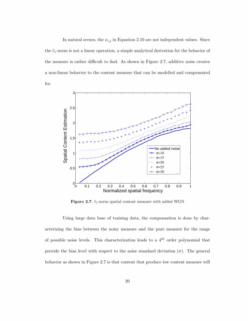
The content figure is obtained from the matrix Y using Equation 2.6. In the simple

case where the image data is only white Gaussian noise, the content measure has a

pure linear behavior with σ2.

µy = E(yi,j) = 2σ2p∑

m=−p

p∑l=−p

α|m|+|l|

= 2σ2

⎡⎣

(21 − α(p+1)

1 − α

)2

− 1

⎤⎦ (2.11)

σ2y = V AR(yi,j) = 12σ4

p∑m=−p

p∑l=−p

α2|m|+2|l|

= 12σ4

⎡⎣

(21 − α(2p+2)

1 − α2

)2

− 1

⎤⎦ (2.12)

Figure 2.6 is the simulation result of the �2-norm spatial content measure for

WGN content with varying standard variation.

Figure 2.11 shows the behavior of the �2-norm measure with linearly increas-

ing content as well as with added noise in different levels. The behavior of the �2-norm

measure is very similar to the �1-norm in terms of correlation of the measure to the

23

0 5 10 15 20 25 30 350

2

4

6

8

10

12

14

Noise standard deviation

Squ

are

root

of c

onte

nt m

easu

re

Figure 2.10: �2-norm spatial content measure behavior for WGN content

content. However, the noise effect on the measure is mainly bias which makes the

noise compensation easier.

Although the �2-norm operation provides good measure of content and it is

robust with noise, it does not have a direct correlation to the statistical model of

the differences between adjacent pixel values as the �1-norm provides. Moreover, it is

computationally more expensive due to the power operation.

2.2 Temporal content measure

Measuring of the temporal content in a video sequence is the companion

problem to the spatial content measure in an image. Here we quantify the temporal

information in the scene. The same �1-norm method as in the spatial case can be used

24

0 0.2 0.4 0.6 0.8 1 0 0.2 0.4 0.6 0.8 0

50

100

150

200

250

300

350

400

450

500

Normalized spatial frequency

Spa

tial c

onte

nt m

easu

re

σ=10σ=20σ=30

No added noise

Figure 2.11: �2-norm spatial content measure with added WGN

on a one dimensional window along the time axis in the following form:

qi,j,t =p∑

k=−p

β|k| |xi,j,t − xi,j,t+k| (2.13)

where the operation is performed on a window of duration 2p + 1 time samples and

the scalar weight 0 < β < 1 is applied to give a temporally decaying effect to the sum-

mation, effectively giving bigger weight to higher temporal frequencies. The window

operation for p = 2 with the decaying factors is illustrated in Figure 2.12. The dif-

ferences are taken between the center pixel and the neighboring pixels in the window

and weighted by the corresponding decaying factor. An alternative operation to the

�1-norm in Equation 2.13 is the �2-norm operation as described in Section 2.1.3.

The content figure is given by ρ(Qt) where Qt is the matrix notation for qi,j,t

25

t

Figure 2.12: The temporal window and the decaying factors of the �1-norm temporal contentmeasure

(at frame t) and the same ρ(·) operator as defined in Equation 2.6 is used to compute

the temporal content measure. The �1-norm operation on the one dimensional window

provides the same linear behavior with noise only sequence as given in Equations 2.14

and 2.15 and shown in Figure 2.13.

µq = E(qi,j,t) =√

4π

σp∑

k=−p

β|k|

=√

4π

σ

[21 − β(p+1)

1 − β− 1

](2.14)

σ2q = V AR(qi,j,t) = 2σ2

p∑k=−p

β2|k|

= 2σ2

[21 − β(2p+2)

1 − β2− 1

](2.15)

26

0 5 10 15 20 25 300

0.5

1

1.5

2

2.5

3

3.5

4

4.5

Noise standard deviation

Tem

pora

l con

tent

mea

sure

Figure 2.13: �1-norm temporal content measure behavior for WGN content

Figure 2.14 is the simulation results of the temporal �1-norm content mea-

sure on synthesized sequences. It also shows the behavior of the measure to added

WGN with different variance levels. The synthesized sequences were composed with

a known temporal frequency content by changing the pixels value along the time axis

using a sinusoid. Figure 2.15 is an example of pixels value along the time axis from

four different sequences. Each sequence has different temporal content according to

the sinusoid being used. The measure characteristics with respect to additive noise,

correlation to the content bandwidth, and behavior with the existence of aliasing, are

similar to its counterpart in the spatial domain.

27

0 0.1 0.2 0.3 0.4 0.5 0.6 0.7 0.8 0.9 10

1

2

3

4

5

6

σ=10σ=15 σ=20 σ=25 σ=30 .

Normalized temporal frequency

Tem

pora

l con

tent

mea

sure

No added noise

Figure 2.14: �1-norm temporal content measure with added WGN

0 20 40 60 80 100 120 140 1600

200

400

0 20 40 60 80 100 120 140 1600

200

400

0 20 40 60 80 100 120 140 1600

200

400

Pix

el v

alue

0 20 40 60 80 100 120 140 1600

200

400

Frame number

Figure 2.15: Pixels value along the time axis of synthesized sequences for the evaluation ofthe temporal content measure

28

Chapter 3

Sensor operating point

In Chapter 2 we explored the means to measure the spatial and temporal content in

the scene using the data retrieved from the sensor. Although not directly, the content

measure dictates the required sampling rate of the scene. The required sampling rate

is used to adjust the temporal and spatial operation of the sensor according to its

capabilities. In this chapter we define the operating point and operating space of the

sensor. We give the means to convert the �1-norm content measure to the required

operating point and describe the projection operation of that point to the sensor

operating space.

3.1 Operating point definition

The sensor operating point (SOP) is defined as {number of pixels per frame,

frame rate} point in the feasible space of the sensor as depicted, for example, in

Figure 3.1. The sensor’s operating space is different from sensor to sensor and may

not be smooth due to physical limitations such as circuit timing and limited inter-

polation capabilities that are required for non-integer spatial sampling rates. The

29

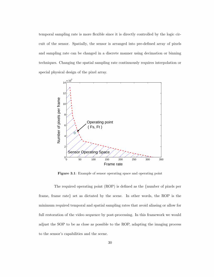
temporal sampling rate is more flexible since it is directly controlled by the logic cir-

cuit of the sensor. Spatially, the sensor is arranged into pre-defined array of pixels

and sampling rate can be changed in a discrete manner using decimation or binning

techniques. Changing the spatial sampling rate continuously requires interpolation or

special physical design of the pixel array.

0 50 100 150 200 250 300 3500

2

4

6

8

10

12

14x 10

5

Frame rate

Num

ber

of p

ixel

s pe

r fr

ame

Sensor Operating Space

∗

Operating point ( Fs, Ft )

Figure 3.1: Example of sensor operating space and operating point

The required operating point (ROP) is defined as the {number of pixels per

frame, frame rate} set as dictated by the scene. In other words, the ROP is the

minimum required temporal and spatial sampling rates that avoid aliasing or allow for

full restoration of the video sequence by post-processing. In this framework we would

adjust the SOP to be as close as possible to the ROP, adapting the imaging process

to the sensor’s capabilities and the scene.

30

3.2 Operating point computation

The ROP is derived from the spatial and temporal content measures. Ideally,

the spatial content measure would be computed by a spatially high resolution sensor

to obtain an accurate non-aliased measure. Similarly, the temporal content would

be ideally measured by a high frame rate sensor such that the temporal information

in the scene is measured accurately. The actual imaging would be done by a third

sensor that is running at varying operating points. A block diagram for such a sensor

is depicted in Figure 1.4. The three-sensor configuration may be too expensive in

practical applications and requires relatively complicated optics. In practice we would

like to measure the content in the scene using the same sensor that is used for imaging.

This may reduce the accuracy of the content measure due to possible aliasing. Using

the �1-norm content measure, the single sensor accuracy problem will only effect the

operating point transitions when significant content changes occur in the scene. The

system will always converge to the correct operating point as further discussed in this

section and in Chapter 4.

The spatial and temporal content measures produce two scalar figures for

each frame of the video sequence. The content measure is the output of the �1-

norm operation and does not have a direct relation to the required sampling rate.

The conversion from content measure to ROP is done through the use of synthesized

video sequences with known spatial and temporal bandwidth. Taking these sequences

through the content measure operations we create spatial and temporal conversion

31

curves.

We show an example of the operating point computation where we take syn-

thesized video and compute the content measures from it. For the spatial conversion,

the sequence is composed of zoneplate images as described in Section 2.1.1 but with

single frequency content for maximum accuracy. The temporal operating point com-

putation is done through a similar concept in the time axis. The synthesized sequences

for the temporal case are described in Section 2.2 and shown as example in Figure 2.15.

Since the characteristics of the conversion are different from one operating

point to another, we use a separate conversion curve for each operating point. Figure

3.2 shows the spatial content measure to required sampling rate conversion curves.

Figure 3.3 shows the conversion curves for the temporal case. The curves that are

presented in those figures are for pre-defined discrete operating points. The simulation

for creating the curves uses a high sampling rate non-aliased sequence as the baseline

and creates lower sampling rate sequences by down sampling. The down-sampled

sequences introduce aliasing as expected.

As shown in Figure 3.2, the spatial content measure for an aliased image will

saturate the �1-norm operator, indicating that the current sampling rate is insufficient.

This characteristic is essential for the closed loop operation of the adaptive sensor as

described in Chapter 4. The temporal conversion in Figure 3.3 has the same saturation

characteristic with additional bias effect. The bias effect is caused by the motion

scaling that takes place in the temporal down sampling action (motion will be larger

between two consecutive frames of the down sampled sequence as compared to the

32

original sequence). If an imaging sensor supports continuous operating points within

its operating space, then Figures 3.2 and 3.3 are the actual conversion to the required

sampling rate. If the sensor supports only discrete points within its operating space,

we can create a look-up table for the conversion by setting thresholds in the conversion

curves at these discrete points.

0 200 400 600 800 1000 12000

0.5

1

1.5

2

2.5

3

3.5

Minimum horizontal and vertical sampling rates

Spa

tial c

onte

nt m

easu

re

Non aliased sequencex2 down sampledx4 down sampledx8 down sampled

Figure 3.2: Spatial content measure to sampling rate conversion

3.3 Projection to the sensor operating space

The required operating point reflects the minimum required sampling rate as

dictated by the scene. In some cases this point falls within the sensor operating space,

but in other cases the ROP may fall outside. These two cases are depicted in Figures

3.4 and 3.5 respectively. In the closed loop operation we need to determine the new

33

0 20 40 60 80 100 120 1400

2

4

6

8

10

12

Minimum frame rate

Tem

pora

l con

tent

mea

sure

No Downsamplingx2 down sampledx4 down sampledx8 down sampledx16 down sampled

Figure 3.3: Temporal content measure to sampling rate conversion

sensor operating point (SOP) for every frame.

In the case where the operating point falls inside the sensor operating space,

there are two options for determining the new sensor operating point. If the objective

is to minimize the bandwidth at the output of the sensor then ROP=SOP. That is

because the ROP is computed from the content measure that obtains the minimum

required sampling rate. In the case where the data bandwidth is second in priority, the

SOP can be shifted (if possible) to higher sampling rates above the minimum defined

by the ROP. The shift can be done in the temporal, spatial or both axes depending

on the available bandwidth and user preferences. This shift is depicted by the dashed

arrows in Figure 3.4. Here we refer to user preferences as the option to shift the

34

operating point towards higher temporal or spatial sampling rate when the option

exists. That allows the user to create a sequence that has higher temporal or spatial

quality respectively.

In the case where the operating point falls outside the sensor operating space,

the sensor does not have sufficient bandwidth to capture the scene and additional

projection operation is required. The most natural projection is to the closest possible

operating point in the sensor operating space as depicted in Figure 3.5. Here again the

user can bias the projection toward higher spatial or temporal sampling rate. However,

in this case the bias will improve the sampling rate of one domain at the expense of

the other.

0 50 100 150 200 250 300 3500

2

4

6

8

10

12

14x 10

5

Frame rate

Num

ber

of p

ixel

s pe

r fr

ame

Sensor Operating Space

∗SOP=ROP

Figure 3.4: Projection of operating point to sensor operating space - point is within the space

35

0 50 100 150 200 250 300 3500

2

4

6

8

10

12

14x 10

5

Frame rate

Num

ber

of p

ixel

s pe

r fr

ame

Sensor Operating Space

∗ROP

SOP ∗

Figure 3.5: Projection of operating point to sensor operating space - point is outside thespace

36

Chapter 4

Closed loop operation

In previous chapters we introduced the content measures and the sensor operating

point and gave the way to obtain them from the sensor data. In this chapter we

describe the closed loop operation of an adaptive sensor. Adaptive imaging can be

described as a control system as it has a proper feedback loop that adjust the system

to track the scene. A real-time experiment in open loop was conducted for the evalua-

tion of the content measures and possible approaches for the operating point feedback

operation. The experiment is presented in Section 4.2. A complete closed loop sim-

ulation of an adaptive imaging sensor was created and the results are presented in

Section 4.3.

4.1 Adaptive imaging control system

Adaptive imaging can be depicted as a control system that tracks the scene

through measuring its content. As illustrated in Figure 4.1, the sensor’s output is

the system output as well as the feedback loop mechanism’s input. The information

about the scene is extracted in the first step of the feedback loop by the content

37

measure block. The content measure is converted to the required operating point

using conversions curves or look-up tables that were prepared according to the imaging

sensor capabilities as described in Section 3.2. The computed operating point may or

may not be within the sensor’s operating space. Therefore, an additional stage of

projecting the required operating point to the sensor operating space is required. The

projection operation is described in details in Section 3.3.

Finally the error in the system between the current operating point and the

computed one is determined and fed back to the sensor through a feedback filter. The

filter in the feedback loop is effectively smoothing the feedback response and keeps

the system from diverging. In a sensor with discrete operating point, the filter can be

as simple as restricting the change in the operating point to the nearest one in any

direction. For a continuous operating space sensor the filter can perform a smoothing

operation as follows,

SOP(t) = SOP(t − 1) + ∆SOPc(t) (4.1)

where SOPc is the SOP that was calculated at time t and ∆ operates as a gain,

controlling the amount of smoothing on the operating point behavior. The sensor

operation normally starts in a middle range operating point and converges within few

frames. The rate of convergence depends directly on the feedback filter gain.

As described in Chapter 3, the ROP to sampling rate conversion will satu-

rate whenever the content is aliased for the current operating point. This important

characteristic of the conversion will ensure the convergence of the system since the

38

saturated value will drive the sensor to a higher sampling rate until no aliasing occur

and the content measure is accurate again or until the sensor has reached its limits.

The convergence speed mainly depends on the feedback loop gain and filter

design. The optimal evaluation will be with a sensor that has continuous operating

space. In the closed loop simulation we use discrete operating points due to limi-

tation in the process of creating the sensor operating space. In this case the filter

simply restricts the operating point to do one step at the time spatially or temporally.

Therefore, the convergence is guaranteed to be within δ frames, where δ is the discrete

distance between the current and the new operating point.

Content

Measure

Feedback

Filter

Content

Measure to

Sampling Rate

Conversion

Adaptive

Imaging

Sensor

New SOP

Data Out

Required SOP

ROP

Projection to the

Sensor’s

Operating Space

+

-

Current SOP

Scene

Figure 4.1: Closed loop operation

4.2 Real-time open loop experiment

The adaptive sensor relies on real-time data processing for the capture of

the scene content. In order to evaluate the robustness of the content measures as

well as the SOP computation, a real time setup was developed. The setup includes a

39

IEEE1394 camera and a PC. The Windows drivers for the camera were obtained from

the robotics institute at Carnegie Mellon university [6].

The purpose of this driver set is to provide easy, direct access to the controls

and imagery of compliant cameras on the IEEE1394 serial bus [1]. These cameras

are capable of transmitting image data at up to 400 mbps while also offering the

ability to control myriad parameters of the camera from software. Having the drivers

and application source code available, the frames from the camera are captured by

relatively minor chances in the software. Additional control can be added to the

user interface for parameter changing in real-time manner. Since the data from the

sensor is captured with no compression, the data can be processed with no additional

artifacts and displayed in real-time. The real-time processing capability depends on the

particular PC performance being used and the complexity of the processing software.

This setup provides a powerful tool for development and testing of image processing

algorithms.

In this experiment we used a Pyro webcam from ADS technologies [20] which

seamlessly connects to the CMU drivers and provides a wide variety of video resolutions

and control. The spatial and temporal content measures were implemented to work

in real-time and give a graphical display of the results. The camera was running at

a constant rate of 320×240 spatially and 30 frames per second temporally. The user

interface is providing control over the measure parameters such as the decaying factors

α and β and the window size of the content measures. Screen capture of the Windows

environment is shown in Figure 4.2. The specific control panel that was created for

40

this experiment is shown in Figure 4.3.

Figure 4.2: Video and graphic display of the IEEE1394 real-time experiment

The real-time graphic display and control proved the robustness of the content

measures throughout various scenes and conditions. Both the temporal and spatial

measures were tested with natural indoors and outdoors scenes to check the correlation

of the measure to the content and behavior with noise. A simple conversion from the

content measure to sensor operating point was manually created using look-up table of

10×10 entries. The new operating point is graphically displayed for the evaluation of

possible approaches towards the development of the content measure to sampling rate

conversion as being used in the closed loop operation. This experiment mainly provides

41

Figure 4.3: Content measure control window of the IEEE1394 real-time experiment

a setup for varying the different parameters in different conditions and observing the

behavior of the content measure and operating point.

Using a more sophisticated camera such as PL-A742 of PixeLink [19] or Mo-

tionXtra HG-SE of Redlake [3], this real-time open loop experiment can be extended

to work in closed loop and provide an adaptive imaging system that can be controlled

by a user through the PC. The data can be stored for post processing or can be post

processed at real-time if computation permits.

4.3 Closed loop simulation

The complete closed loop system was simulated using real sequences from

a high definition television video source. The high definition video is composed of

1920×1088 images at 60 frames per second frame rate. By down-sampling this se-

quence spatially and temporally, we created several discrete operating points as de-

picted in Figure 4.4. Since the original sequence is sampled at high sampling rate

42

spatially and temporally, the down sampling operation could be done using integer

values only and avoiding any interpolation that could warp the data. The operat-

ing space of this simulated sensor is large enough to demonstrate the transitions in

operating points and system convergence.

0 10 20 30 40 50 60 70

0.5

1

1.5

2

2.5x 10

6

Frame rate

Num

ber

of p

ixel

s pe

r fr

ame

original operating point

discrete operating points

Figure 4.4: Operating space created for the closed loop simulation

The conversion from ROP to sampling rate has been tabulated using thresh-

olds as described in Chapter 3. For the spatial conversion we use the curve in Figure

3.2 and set the thresholds at the discrete operating points available for the simula-

tion. Similarly, the temporal conversion is using the curve from Figure 3.3. The

system output was evaluated through a simple display mechanism where images were

spatially scaled and temporally repeated to create a high spatio-temporal sampling

43

rate sequence. The simulation output results in a new sequence that has significantly

reduced data bandwidth at certain points. The bandwidth reduction can be as sig-

nificant as 40% of the original sequence for static scenes or scenes with low spatial

bandwidth. The operating point dynamics show high correspondence to the image

bandwidth as measured in the frequency domain.

Figures 4.5(a) and (b) are the spatial and temporal content measures along

900 frames of a high definition video sequence. We marked the major operating point

transitions along the curves and show the corresponding images in Figure 4.6. The

sequence is a football match that starts from almost a static scene with relatively low

content. The operating point converges at that point to the lowest spatio-temporal

sampling rate (first image). The next operating point transition to a higher sampling

rate happens when the players move to their position (second and third images). Once

the players are in place, the scene is less active and the camera zooms out getting more

spatial details to the scene. At that point, the operating point has higher spatial and

lower temporal sampling rates (fourth image). When the play starts, the temporal

sampling rate increases rapidly (fifth and sixth images) and settles back down for the

rest of the sequence (seventh and eighth images).

44

100 200 300 400 500 600 700 800 900 10000

0.2

0.4

0.6

0.8

1

1.2

Frame number

Spa

tial c

onte

nt m

easu

re

272x

480

272x

480

136x

240

272x

480

544x

960

272x

480

272x

480

136x

240

100 200 300 400 500 600 700 800 900 10000

1

2

3

4

5

6

7

Frame number

7.5F

PS

15F

PS

30F

PS

15F

PS

30F

PS

60F

PS

30F

PS

30F

PS

Tem

pora

l con

tent

mea

sure

(a) Spatial content measure (b) Temporal content measure

Figure 4.5: Spatial and temporal content measures of the football sequence

(1) 136x240 7.5fps (2) 272x480 15fps (3) 272x480 30fps (4) 544x960 15fps

(6) 136x240 60fps (7) 272x480 30fps (8) 272x480 30fps (5) 272x480 30fps

Figure 4.6: Input images from the football sequence at the operating point transitions.The numbers below each picture indicate the computed operating points of the closed loopoperation.

45

Chapter 5

Conclusions and future work

In this thesis we have presented a novel approach for image and video sensing. Imaging

is done with adaptation to the spatial and temporal content of the scene, optimizing

the sensor’s sampling rate and the camera transmission or storage bandwidth. We

developed a spatial and temporal content measure based on an �1-norm and charac-

terized it with respect to noise, image bandwidth, and aliasing. Real-time open loop

experiment was conducted using an IEEE1394 camera and a PC. The experiment

shows the real-time response of the content measures as well as possible dynamics of

the operating point. A complete closed-loop system has been simulated using TV high

definition video and the results show high correspondence to the scene dynamics and

results in significant reduction in the camera output bit-rate.

The output of an adaptive sensor is a sequence of images with varying spatial

and temporal sampling rates. This data stream captures the scene more efficiently

and with fewer artifacts such that in a post-processing step an enhanced resolution

sequence can be composed or lower bandwidth can be used. Having the scene optimally

46

sampled within the sensor capabilities, the post processing step actually enhance the

sequence beyond the sensor operating space. The non-standard stream requires a non-

traditional mechanism to address the change in sampling rate. The post processing

step can be part of future work in this framework for adaptive imaging.

Well established video processing methods such as super-resolution [8] and

motion compensated interpolation [17] are very appropriate for restoring a spatio-

temporal high resolution sequence from adaptively captured data. Video super-resolution

can take the raw data from the sensor and restore a spatially higher resolution sequence

by using data from neighboring frames. Motion compensated interpolation can fill-up

the missing frames temporally.

An adaptive sensor system can send additional information to the post-

processing engine to allow for an easier, higher quality restoration. This information

can include the operating point, a measure for the amount of aliasing, or the content

measure itself. In a three sensor configuration, additional information for the motion

in the scene can be extracted from the high temporal sampling rate sensor. In systems

where compression mechanism such as MPEG encoder already exist, one can think of

using the motion estimation and DCT computation as ways to obtain measure of the

content and to use it to compute operating point and feed it back to the sensor.

In a complete system where a post-processing stage restores the sequence, a

second feedback loop from the post processor to the adaptive sensor can be added.

This feedback will use quality measures on the restored sequence and will tune up the

adaptive sensor settings to achieve maximum performance. Some of the parameters

47

that can be tuned include the α, β, and η coefficients of the content measure, conversion

curves or look-up tables, temporal or spatial bias in the projection process to the sensor

operating space, and the filter gain and behavior in the feedback loop.

The adaptive framework incorporates simple computation that can be im-

plemented as a hardware module within the sensor. In CMOS sensors the adaptive

circuit can reside on the same silicon and for CCD devices it can be part of the uni-

versal timing generator (UTG) used with any CCD. A possible prototype system for

the adaptive sensor can use an existing camera such as the PL-A742 of PixeLink and

field programmable gate array (FPGA) for the adaptive circuit and a simple post pro-

cessing. The output of the system can drive a display directly or stream the raw data

to a PC for storage and evaluation.

48

Appendix A

Simulation environment

In this appendix we present the Matlab simulation environment that was developed

for the adaptive image and video sensing. The Matlab routines that are mentioned in

the appendix can be retrieved from the Multi-Dimensional Signal Processing research

group in the electrical engineering department in the University of California, Santa

Cruz. The simulation environment takes as an input raw high definition video data.

It creates spatially down sampled sequences at discrete pre-defined resolutions and use

them to create the output from the adaptive sensor. The down-sampled video data

is processed through the content measures, the operating point computation, and a

feedback loop mechanism that defines the next frame to use from the down sampled

data at any iteration of the simulation.

High definition source is usually available in MPEG2 program or transport

stream formats as it comes through the cables or terrestrial broadcasting. The video

sampling rate for high definition is normally 1920×1088 at 60 fields per second (1080i)

or 1280×720 at 60 frames per second (720p). Decoding the high definition video to a

49

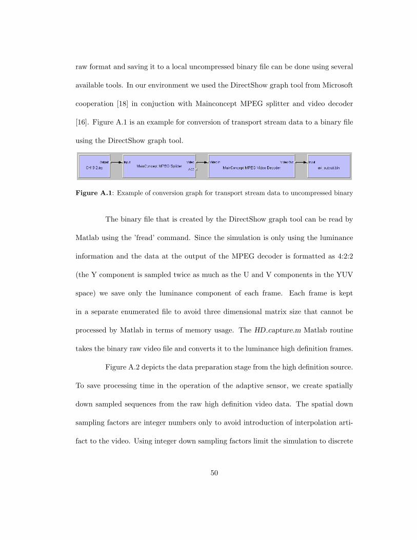
raw format and saving it to a local uncompressed binary file can be done using several

available tools. In our environment we used the DirectShow graph tool from Microsoft

cooperation [18] in conjuction with Mainconcept MPEG splitter and video decoder

[16]. Figure A.1 is an example for conversion of transport stream data to a binary file

using the DirectShow graph tool.

Figure A.1: Example of conversion graph for transport stream data to uncompressed binary

The binary file that is created by the DirectShow graph tool can be read by

Matlab using the ’fread’ command. Since the simulation is only using the luminance

information and the data at the output of the MPEG decoder is formatted as 4:2:2

(the Y component is sampled twice as much as the U and V components in the YUV

space) we save only the luminance component of each frame. Each frame is kept

in a separate enumerated file to avoid three dimensional matrix size that cannot be

processed by Matlab in terms of memory usage. The HD capture.m Matlab routine

takes the binary raw video file and converts it to the luminance high definition frames.

Figure A.2 depicts the data preparation stage from the high definition source.

To save processing time in the operation of the adaptive sensor, we create spatially

down sampled sequences from the raw high definition video data. The spatial down

sampling factors are integer numbers only to avoid introduction of interpolation arti-

fact to the video. Using integer down sampling factors limit the simulation to discrete

50

operating points along the sensor operating space as depicted in Figure 4.4. Temporal

down sampling in the operation of the adaptive sensor is done in the closed loop simu-

lation by picking the right frame index from these spatially down sampled sequences.

The HD2sampled seqs.m Matlab routine creates the down sampled sequences from the

high definition raw video data.

Spatial Down Sampling

1920x1088

960x544480x272 240x136

Figure A.2: Sensor operating space preparation from high definition video source

The adaptive sensor simulation uses four spatial operating points and four

temporal operating points as created by the down sampling routine. Certain com-

binations of the spatial and temporal points creates the sensor operating space as

depicted in Figure 4.4. The simulation starts at the 480×272, 30 frames per second

51

operating point. The spatial content measure is performed on each frame using the

L1 spatial content measure.m Matlab routine, with nominal settings of α = 0.5 and

window size p = 2 . The temporal content measure is performed on sets of 2p + 1

frames using the L1 temporal content measure.m Matlab routine, with nominal set-

tings of β = 0.5 and window size p = 2.

The content measures are converted to required operating point by using look-

up tables that were created from the conversion curves as described in Chapter 3. The

projection to the sensor operating space is simply done by choosing the nearest point in

the space and restricting the change to be no more than one step up or down spatially

or temporally. Once the new operating space is found we submit a new frame from the

right down sampled sequence at the right time index to the output of the sensor. As a

final stage we create an avi file of the adaptive sensor output to evaluate the adapted

sequence along with the corresponding content measures presented side by side with

the images. This closed loop operation is implemented in the closed loop operation.m

Matlab routine and depicted in Figure A.3.

52

SpatialContentMeasure

ContentMeasure to

Sampling RateConversion

Projection toNearest

Operating point

TemporalContentMeasure

ContentMeasure to

Sampling RateConversion

ApplyRestrictions

(filtering)

Get New FrameCreate

AVI

SOP

Figure A.3: Block diagram of the closed loop simulation environment

53

Bibliography

[1] IEEE1394 Trade Association,http://www.1394ta.org/Technology/Specifications/specifications.htm.

[2] M. Ben-Ezra and S. K. Nayar, Motion-based motion deblurring, IEEE Transac-tions on Pattern Analysis and Machine Intelligence 26 (2004), no. 6.

[3] Redlake High-Speed Motion Cameras, http://www.pixelink.com/.

[4] C.E.Shannon, A mathematical theory of communication, Bell Syst. Tech. J. 27(1948), 379–423, 623–656.

[5] T. Chen, Digital camera system simulator and applications, Ph.D. thesis, StanfordUniversity, EE Department, 2003.

[6] CMU 1394 Digital Camera Driver, http://www-2.cs.cmu.edu/∼iwan/1394/.

[7] M. Elad, On the bilateral filter and ways to improve it, IEEE Transactions onImage Processing 11 (2002), no. 10, 1141–1151.

[8] S. Farsiu, D. Robinson, M. Elad, and P. Milanfar, Fast and robust multi-framesuper-resolution, IEEE Transactions on Image Processing 13 (2004), 1327–1344.

[9] M. Green, Statistics of images, the tv algorithm of rudin-osher-fatemi for imagedenoising and an improved denoising algorithm, UCLA CAM Report (2002), 02–55.

[10] G. E. Healey and R. Kondepudy, Radiometric ccd camera calibration and noiseestimation, IEEE Transactions on Pattern Analysis and Machine Intelligence 16(1994), no. 3.

[11] S. Kullback, Information theory and statistics, Tech. report, Dover Publications,Inc, 1968.

[12] S. H. Lim, Video processing applications of high speed cmos sensors, Ph.D. thesis,Stanford University, EE Department, 2003.

54

[13] A. Papoulis and S. Unnikrishna Pillai, Probability, random variables and stochas-tic processes, McGraw-Hill, 2001.

[14] E. Shechtman, Y. Caspiand, and M. Irani, Increasing space-time resolution invideo, Proceedings of the Seventh European Conference in Computer Vision 1(2002), 753.

[15] H.R. Sheikh and A.C. Bovik, Image information and visual quality, Proceedingsof the IEEE International Conference on Acoustics, Speech, and Signal Processing3 (2004), 709–12.

[16] MainConcept Multimedia Technologies, http://www.mainconcept.com/.

[17] A. M. Tekalp, Digital video processing, Prentice-Hall, 1995.

[18] Microsoft Cooperation DirectShow Graph Tool, http://msdn.microsoft.com/.

[19] PixeLink Machine Vision, http://www.adstech.com/.

[20] Pyro webcam from ADS tech, http://www.adstech.com/.

[21] J. Yang-Pelaez and W. C. Flowers, Information content measures of visual dis-plays, Proceedings of the IEEE Symposium on Information Vizualization (2000).

[22] H. You, Q. Zhu, and A. Alwan, Entropy-based variable frame rate analysis ofspeech signals and its application to asr, ICASSP, Montreal, Canada (2004).

[23] Q. Zhu and A. Alwan, On the use of variable frame rate analysis in speech recog-nition, ICASSP (2000), 3264–3267.

55