an analyis of processing and distribution productivity … · an analysis of processing and...
TRANSCRIPT

Farm FreshDairy Products
Farm FreshDairy Products
Farm Fresh Dairy ProductsMILK 1
Greenville Dairies
An Analysis of Processing and Distribution Productivity and Costs in 35 Fluid Milk Plants
Eric M. ErbaRichard D. Aplin
Mark W. Stephenson
A Publication of the
Cornell Program on Dairy Markets and Policy
Department of Agricultural, Resource and Managerial EconomicsCollege of Agriculture and Life Sciences
Cornell UniversityIthaca, NY 14853-7801
February 1997 R.B. 97– 03
1% Lowfat
Milk
RealDairy Creamer
GreenvilleDairies
GreenvilleDairies
GreenvilleDairies
SkimMilk
Milk
1% LowfatMilkMilk

i
Table of ContentsSubject Page
Acknowledgments ........................................................................................................ viHighlights .................................................................................................................... viiIntroduction ................................................................................................................... 1
Objectives ........................................................................................................... 1Profile of fluid milk operations studied ................................................................ 1Data collection period ......................................................................................... 1
Background information on fluid milk plants ............................................................ 2History and description of fluid milk plants ......................................................... 2Previous studies of fluid milk plants ................................................................... 3Using boxplot to report results............................................................................ 4
Outline of report ....................................................................................................... 4
Section I: General characteristics of plants studied ..................................................... 5Plant location and ownership ............................................................................. 5Volumes processed ............................................................................................ 5Plant capacities .................................................................................................. 5Number of products, labels processed, and SKUs processed ........................... 7Plant and cooler evaluation ................................................................................ 7Plastic jug filling equipment ................................................................................ 8Paperboard filling equipment.............................................................................. 9Product handling in the cooler and product loading ......................................... 10
Plant labor productivity .......................................................................................... 11Plant labor costs .................................................................................................... 12
Hourly cost of labor .......................................................................................... 11Fringe benefits.................................................................................................. 12Labor cost per gallon ........................................................................................ 12
Cost of utilities ....................................................................................................... 13Plant costs ............................................................................................................. 14
Plant cost per gallon ......................................................................................... 15Purchased packaging materials............................................................................. 16Blow mold operations ............................................................................................ 17
Blow mold labor productivity............................................................................. 17Cost of resin per pound .................................................................................... 18Cost of producing a jug .................................................................................... 18
Section II: Determining the impact of various factors on labor productivityand cost per gallon.................................................................................... 19
Overview .......................................................................................................... 19Developing measures to analyze fluid milk plants............................................ 19Selecting the independent variables ................................................................ 20Other possible variables to consider ................................................................ 21Model specification ........................................................................................... 22Pooling cross-section and time-series data ...................................................... 23

ii
Subject Page
Contemporaneous correlation and recursive systems ..................................... 24Interpreting results of the analyses .................................................................. 25
Results of the analyses .......................................................................................... 25Plant labor productivity ..................................................................................... 25
Overview of results ..................................................................................... 25Plants owned by supermarket companies .................................................. 26Labor cost per hour ..................................................................................... 27Container mix .............................................................................................. 27Plant capacity utilization .............................................................................. 27Number of SKUs and product handling ...................................................... 28Level of automation..................................................................................... 28Size of plant ................................................................................................ 28Comparing regression and neural network results ..................................... 29Unionization ................................................................................................ 30
Processing and filling labor productivity ........................................................... 30Overview of results ..................................................................................... 30Plant size .................................................................................................... 31Plants owned by supermarket companies and milk cooperatives .............. 31Labor cost per hour ..................................................................................... 31Container mix .............................................................................................. 32Plant capacity utilization .............................................................................. 32Level of automation..................................................................................... 32Number of SKUs ......................................................................................... 32
Cooler and load out labor productivity .............................................................. 32Overview of results ..................................................................................... 32Plant size .................................................................................................... 33Plants owned by supermarket companies and milk cooperatives .............. 34Labor cost per hour ..................................................................................... 34Container mix .............................................................................................. 34Product handling and SKUs stored in the cooler ........................................ 35Level of automation..................................................................................... 35
Plant cost per gallon ......................................................................................... 35Overview of results ..................................................................................... 35Plants owned by supermarket companies .................................................. 37Labor cost per hour ..................................................................................... 37Plant size and plant capacity utilization ...................................................... 38Level of automation..................................................................................... 38Population density ....................................................................................... 38Factors that affect cost indirectly ................................................................ 39Comparing regression and neural network results ..................................... 39
Section III: Characteristics of fluid milk distribution operations .................................. 40Types of wholesale routes ................................................................................ 40Size of wholesale customers ............................................................................ 41Cost of delivery implements ............................................................................. 42

iii
Subject Page
Description of specialized routes ........................................................................... 43Frequency of delivery to large accounts........................................................... 43Delivery methods for large accounts ................................................................ 44Type of driver compensation ............................................................................ 44Delivery vehicles .............................................................................................. 45
Characteristics, productivity and costs of specialized routes................................. 46Number of cases, number of stops and miles travelled ................................... 47Driver labor productivity .................................................................................... 47Cost of driver labor per hour............................................................................. 47Cost of labor per case ...................................................................................... 48Direct delivery cost per case ............................................................................ 48
Section IV: Factors causing route labor productivity and costs to vary ...................... 49Overview .......................................................................................................... 49Developing measures to test ............................................................................ 49Selecting the independent variables ................................................................ 50Notes on distribution data ................................................................................. 50Model Specification .......................................................................................... 51Statistical notes ................................................................................................ 51
Results of the analyses .......................................................................................... 52Route labor productivity .................................................................................... 52
Overview of results ..................................................................................... 52Routes operated by captive plants.............................................................. 52Labor cost per hour ..................................................................................... 53Miles travelled ............................................................................................. 53Number of customer stops .......................................................................... 53Product on pallets ....................................................................................... 53Dock deliveries............................................................................................ 54Population density ....................................................................................... 54Unionized labor ........................................................................................... 54
Driver labor cost per case ................................................................................ 55Overview of results ..................................................................................... 55Routes operated by captive plants.............................................................. 55Unionized labor ........................................................................................... 56Population density ....................................................................................... 56Variables that affect costs indirectly ............................................................ 57
Direct delivery cost per case ............................................................................ 57Overview of results ..................................................................................... 57Routes operated by captive plants.............................................................. 59Labor cost per hour ..................................................................................... 59Miles travelled and number of customer stops ........................................... 59Population density ....................................................................................... 59
Section VI: Selling and general and administrative expenses ................................... 60References .................................................................................................................. 62

iv
List of FiguresSubject Page
Figure 1 Gallons processed per month .....................................................................5Figure 2 Percent capacity utilization ..........................................................................6Figure 3 Average percent plant capacity utilization by month ...................................6Figure 4 SKUs processed and SKUs stored in the cooler .........................................7Figure 5 Number of labels packaged ........................................................................7Figure 6 Percent of gallon and half-gallon plastic jug fillers by number
of filling valves .............................................................................................8Figure 7 Filling speed and age of plastic jug fillers ....................................................9Figure 8 Percent of half-gallon, quart, pint, and half-pint carton fillers
by manufacturer ..........................................................................................9Figure 9 Filling speed and age of paperboard carton fillers ......................................9Figure 10 Percent of plants using various product handling systems
in the cooler ...............................................................................................10Figure 11 Percent of respondents using automated product handling systems........10Figure 12 Percent of all distribution routes loaded by various methods .................... 11Figure 13 Plant labor productivity in gallons per hour ............................................... 11Figure 14 Cost of plant labor per hour .......................................................................12Figure 15 Fringe benefits as a percent of wages ......................................................12Figure 16 Labor cost relative to other plant costs......................................................12Figure 17 Labor cost per gallon .................................................................................13Figure 18 Unit costs of fuels ......................................................................................13Figure 19 Cost of utilities per gallon ..........................................................................14Figure 20 Plant cost per gallon ..................................................................................15Figure 21 Breakdown of plant cost per gallon ...........................................................15Figure 22 Net delivered costs for paperboard cartons ..............................................16Figure 23 Net delivered costs for cap and label ........................................................17Figure 24 Jugs per hour of blow mold labor ..............................................................17Figure 25 Resin cost per pound ................................................................................18Figure 26 Cost of producing a plastic jug ..................................................................18Figure 27 Breakdown of the cost of producing a plastic jug ......................................19Figure 28 Plastic jug weights .....................................................................................19Figure 29 Percent of plant volume distributed by various methods........................... 41Figure 30 Miscellaneous distribution information ...................................................... 41Figure 31 Size of wholesale deliveries by percent of customers
and percent of plant volume ...................................................................... 42Figure 32 Weekly frequency of deliveries to large accounts ..................................... 43Figure 33 Percent of plants using various delivery implements on
specialized routes ..................................................................................... 44Figure 34 Methods of driver payment on specialized routes ..................................... 45Figure 35 Miscellaneous specialized route driver information ................................... 45Figure 36 Working load size in cases for vehicles on specialized routes .................. 45Figure 37 Descriptors of specialized routes .............................................................. 46Figure 38 Cases delivered per hour of driver labor ................................................... 47Figure 39 Cost of driver labor per hour ..................................................................... 48Figure 40 Cost of driver labor per case ..................................................................... 48Figure 41 Direct delivery cost per case ..................................................................... 48Figure 42 Selling and G & A costs per gallon ............................................................ 61

v
List of Tables
Subject Page
Table 1 Ratings of plant and cooler characteristics by managers ............................ 8Table 2 Summary statistics for plant efficiency and cost measures ....................... 22Table 3 Regression results for plant labor productivity ......................................... 26Table 4 Regression results for processing and filling labor productivity................. 31Table 5 Regression results for cooler and load out labor productivity.................... 33Table 6 Regression results for plant cost per gallon .............................................. 36Table 7 Total effects of various factors on plant cost per gallon............................. 37Table 8 Costs per unit, life expectancies, and deposits for various
delivery implements................................................................................... 42Table 9 Summary statistics for various factors affecting driver labor
productivity and driver cost per gallon ....................................................... 50Table 10 Regression results for driver labor productivity ......................................... 52Table 11 Regression results for driver labor cost per case ...................................... 56Table 12 Total effects of various factors on driver labor cost per case .................... 56Table 13 Summary statistics for various affecting direct delivery cost per case ...... 57Table 14 Regression results for direct delivery cost per case .................................. 58Table 15 Total effects of various factors on direct delivery cost per case ................ 59

vi
Acknowledgments
Eric M. Erba is a Ph. D. candidate, Richard D. Aplin is a Professor Emeritus, andMark W. Stephenson is a Senior Extension Associate in the Department of Agricultural,Resource, and Managerial Economics at Cornell University.
We would like to thank George Johnson, Jr. (JAI Engineers) of Sarasota, FL and AlHamilton of Somerset, KY for their assistance in several aspects of the study. We wouldalso like to thank James Pratt, Lois Willett, William Tomek, and Andrew Novakovic fromthe Department of Agricultural, Resource and Managerial Economics for their advice andinsightful comments throughout the duration of the study.
We are grateful to the personnel from the participating dairy companies who sacri-ficed many hours to research and report data from all aspects of their respective organiza-tions. Without their efforts, this study would not have been possible.
Finally, we wish to thank Tetra Pak, Inc. for generously providing a portion of thefunding for this research.

vii
HIGHLIGHTS
The study focuses on plant and distribution route labor productivity and costs of 35fluid milk plants in 15 states. We targeted medium and large plants that are well managed andhave a significant market presence. The 35 operations are highly respected in the industryand are thought to be among the best fluid milk operations in the country. Of the 35 plants inthe study, 8 are owned and operated by supermarket companies (i.e., captive plants), 5 areowned and operated by farmer milk marketing cooperatives, and the remaining 22 are inde-pendently owned and operated. Participating plants submitted data from a recent 12-monthperiod. Most plants submitted data from 1993 or 1994 calendar years.
Key Characteristics of Survey Plants
The following table describes key characteristics of the 35 plants. The figures in thecolumn labeled “High 3 Average” (“Low 3 Average”) represent the average values of thehighest 3 (lowest 3) plants calculated for each characteristic. High and low averages for eachcharacteristic were computed independently.
Plant Average Low 3 High 3Characteristic of 35 Plants Average Average
All fluid products, million lbs. per month 27.7 13.3 51.4SKUs processed 148 26 367SKUs in cooler 250 40 539Number of labels 11 2 34Labor cost (including benefits), $ per hour 20.19 13.12 27.92Electricity, ¢ per kwh 6.7 2.2 13.2Natural gas, ¢ per therm 42.6 18.1 66.0Level of processing & filling technology (1 to 10; 10 = highest) 7.4 4 9Level of cooler & load out technology (1 to 10; 10 = highest) 5.9 1 10
Labor Productivity and Costs
We offer the following caveats for the summary of labor productivity and plant costs:
♦ The productivity and unit costs were calculated on a gallon equivalent basis andincluded all beverage products processed and packaged in the plant. Items inaddition to fluid milk products included creamers, juices, drinks, bottled water, andice cream mixes. Soft dairy products, such as yogurt, cottage cheese, and sourcream, were not included.
♦ Labor hours and labor costs reflected direct labor from the raw milk receiving baysthrough the cooler and load out area. Labor assigned to maintenance, plant qualitycontrol, plant office support, and plant management was also included. The blowmold area was excluded from plant cost and productivity measures but was ana-lyzed separately.

viii
♦ Labor hours and labor costs did not include any labor dedicated to production ofsoft products. Raw milk procurement, distribution, selling, and general and admin-istrative expenses were also excluded.
♦ The plant with the highest labor productivity or the lowest cost per gallon was notnecessarily the most profitable. Many factors affect profitability, and we did notattempt to analyze profitability in this report.
Detailed analyses were made of several plant performance measures. Averages andranges are provided in the following table.
Measure of Average Low 3 High 3Performance of 35 Plants Average Average
Gallon equivalents per hour of labor 174 107 286Labor cost, ¢ per gallon 12.3 7.7 17.1Cost of utilities, ¢ per gallon 2.6 1.7 4.2Plant cost, depreciation excl'd, ¢ per gallon 18.2 11.5 24.0Plant cost, depreciation incl'd, ¢ per gallon 21.1 13.1 27.3Gallon jugs produced per hour of blow mold labor 2,244 1,010 5,017Cost of producing gallon jug, ¢ per jug 8.8 7.5 10.3
The next table summarizes the labor productivity and costs in the 35 plants by incre-ments. Each increment, or quartile, represents 25% of the plants. Each line was computedindependently so the 9 plants with the highest labor productivity were not necessarily thesame 9 plants with the lowest costs.
Plant Average of Average of Average of Average ofCharacteristic Lowest 25% Next 25% Next 25% Highest 25%
Gallon equivalents per hour of labor 118 147 178 256Labor cost, ¢ per gallon 8.3 11.2 13.9 16.1Cost of utilities, ¢ per gallon 1.9 2.3 2.7 3.7Plant cost, depreciation excl'd, ¢ per gallon 12.9 17.1 20.5 22.5Plant cost, depreciation incl'd, ¢ per gallon 15.1 20.2 23.3 26.1Gallon jugs produced per hour of blow mold labor 1,221 1,781 2,166 3,932Cost of producing gallon jug, ¢ per jug 8.0 9.1 9.6 9.9

ix
Why Does Plant Cost per Gallon Vary So Widely?
Ten factors were significant in explaining the wide variation in plant cost per gallon(exclusive of depreciation) in the 35 plants. However, the effects of some factors were muchlarger than other factors. The following factors were most important in explaining the widevariation in plant cost per gallon in the 35 plants:
♦ Whether or not the plant was owned by a supermarket chain (captive plant)♦ Level of wages and fringe benefits
The following factors were somewhat important in explaining the variation in plant cost pergallon:
♦ Size of the plant as measured by gallon equivalents processed per month♦ Percent of total volume packaged in gallon and half-gallon containers♦ Extent to which plant capacity was used
Five other factors, although statistically significant, were much less important in explainingvariations in plant cost per gallon:
♦ Level of technology in the processing and filling area♦ Level of technology in the cooler and load out area♦ Number of SKUs processed♦ Location of plant♦ Percent of product handled on pallets
Why Does Plant Labor Productivity Vary So Widely?
Nine factors were significant in explaining the wide variation in plant labor productivityin the 35 plants studied. Seven factors had large and positive effects on plant labor productiv-ity:
♦ Whether or not the plant was a captive supermarket plant♦ Percent of total volume packaged in gallon and half-gallon containers♦ Level of wage rates and fringes♦ Size of plant as measured by gallon equivalents processed per month♦ Extent to which plant capacity was used♦ Level of technology in the processing and filling area
Cooler technology, the number of SKUs processed and the use of pallets were statis-tically significant but had relatively minor effects on plant labor productivity.
Alternative Cost per Gallon and Plant Labor Productivity Results
In a separate Cornell study, the same plant data were analyzed using an increasinglypopular method called neural networks (12). Neural networks “learn” from examples andcan exhibit some capability for generalization beyond the data upon which the network istrained. The “learning” in this context is analogous to “estimation” in more traditionalstatistical analysis. Similarly, “training” data is analogous to “observed” data. We appliedneural network models to plant data to asses the interrelationships among the factorsaffecting plant labor productivity and cost per gallon and to determine if factor effectsdiffered by type of plant ownership.

x
The results of the neural network approach differed slightly from those obtained usingregression analyses. While the analyses revealed strong agreement for most of the factoreffects, other effects showed weak agreement or no agreement at all. For example, bothanalyses predicted positive effects of similar magnitude on labor productivity for captive plants,cost of labor, plant capacity utilization, plant size, and processing technology. For percent ofvolume packaged in gallon and half-gallon containers, percent of plant volume handled onpallets, cooler technology, and SKUs processed, the two techniques showed agreement inthe direction of the impact but differed in terms of the magnitude of the effects. The regres-sion analysis predicted that unionized workforces would be more productive than non-union-ized workforces, but the neural network approach predicted the opposite effect for unionizedlabor. A more comprehensive review of the two sets of results is presented in the sectionsdiscussing the effects of factors on plant labor productivity and plant cost per gallon.
Key Characteristics of Wholesale Route Operations
All 35 plants submitted general information on their distribution operations. On aver-age, over half of the product was distributed by specialized or supermarket routes. Custom-ers served by the plants tended to be large. An average of 43% of the plants' customersordered over 100 cases per delivery and accounted for an average of 64% of the plants'product distribution. The following table summarizes key characteristics of the wholesaleroute operations of the plants.
Route Operation Average Average AverageCharacteristic All Plants Low 3 High 3
Percent of plant volumedistributed by:
♦specialized routes 52 5 100♦ mixed or peddle routes 18 0 71♦ branch, depot, dealer, or
warehouse routes 26 0 47♦other routes 4 0 73
Size of customer:Over 100 cases per delivery
♦ percent of customers 43 1 100♦ percent of volume 64 2 100
Characteristics of Routes Dedicated to Serving Large Accounts
The remainder of the study of distribution operations focused only on “supermarket” orspecialized routes. Specialized routes were defined as routes typically serving 1 to 8 largecustomers, such as supermarkets, club stores, or large convenience stores, per delivery day.Only 20 plants submitted complete surveys on their specialized routes. These 20 plants sub-mitted data on 270 specialized routes. Key characteristics of the 270 specialized routes arepresented in the following table:

xi
Average AverageSpecialized Average All Low 10% High 10%Route Characteristic 270 Routes of Routes of Routes
Cases delivered per month 18,900 10,200 35,000Customer stops per month 97 48 168Miles per month 3,150 745 6,850Driver labor cost (including
benefits), $ per hour $23.39 $16.55 $32.27Product on pallets, % 49 0 100Dock deliveries, % 83 13 100
Specialized Route Labor Productivity and Costs
As you study this summary of route labor productivity and costs, remember that:
♦The route labor productivity and costs only reflect the productivity and costs of routesserving large customers, such as supermarkets and club stores. These routes wouldtypically use tractor-trailers for delivery, and an average of 5 customers per day wereserved by these specialized routes.
♦The cost per case of serving smaller customers, such as small conveniencestores, Mom and Pop stores, delis and restaurants would be much higher thanthe direct delivery costs reported here.
♦The routes with the highest labor productivity or the lowest cost per case were notnecessarily the most profitable. Many factors affect profitability, and we did not at-tempted to analyze profitability in this report.
Average AverageSpecialized Route Average of Low 10% High 10%Characteristic All Plants of Routes of Routes
Cases deliveredper hour of labor* 108 52 216
Driver labor cost,¢ per case* 16.8 10.1 47.8
Direct delivery cost,¢ per case** 36.8 17.3 63.1
* Reflects 270 specialized routes operated by 20 plants.** Reflects 180 specialized routes operated by 15 plants which reported delivery vehicle costs and route labor costs.
Why Does Labor Productivity on Specialized Routes Vary?
While most of the 270 specialized routes studied delivered between 60 and 180 casesper hour, the bottom 10% of the routes averaged only 52 cases per hour. On the other hand,the top 10% of the routes averaged 216 cases per hour.

xii
Five factors were significant in explaining the wide variation in driver labor productivityon the routes dedicated to serving large accounts. However, the effects of some were muchlarger than others. The three most important factors in explaining the variation in driver laborproductivity were:
♦ Whether or not the routes were operated by a supermarket company♦ Combined cost of driver wages and fringe benefits per hour♦ Number of miles travelled per month
Two factors were associated with higher route labor productivity, but were less impor-tant than the three factors listed above:
♦ Higher percentage of product delivered on pallets♦ Higher population density of the city in which the plant is located
Three factors were associated with lower route labor productivity, but were not statisti-cally significant:
♦ Higher number of customer stops♦ Higher percentage of dock-delivered orders♦ Unionized drivers
Why Does Direct Delivery Cost per Case on Specialized Routes Vary?
While most of the 180 specialized routes studied for which vehicle and labor costswere reported fell between 19¢ per case and 58¢ per case, the bottom 10% of the routesaveraged 63¢ per case. On the other hand, the top 10% of the routes averaged 17¢ per case.
Seven factors were significant in explaining the wide variation in direct delivery costper case on the routes dedicated to serving large accounts. The two most important factors inexplaining the variation in direct delivery cost per case were:
♦Whether or not the routes were operated by a supermarket company♦The combined cost of driver wages and fringe benefits
Three factors of moderate importance also affected delivery costs, but were less influ-ential than the two factors listed above:
♦ Miles travelled♦ Number of customer stops♦ Population density of the city in which the plant is located
Two other factors were associated with higher delivery costs, but were less importantthan the five factors above:
♦ Percent of dock-delivered orders♦ Percent of product handled on pallets

1
INTRODUCTION
Objectives
This report details the results of a survey of 35 fluid milk plants and their associateddistribution operations. The objectives of the study were to determine the costs of pro-cessing and distributing fluid milk products and to identify and to quantify the factors whichcontribute to differences in labor productivity, plant cost per gallon, and direct delivery costper case. Specifically, we sought to answer the following questions:
• What are the key characteristics of the fluid milk operations in the study?• What is the average labor productivity and cost per gallon in participating plants,
and how much variation exists in these performance measures?• What factors apparently cause labor productivity and plant cost per gallon to vary
among the 35 plants in the study?• What is the magnitude of the impact on labor productivity and cost per gallon for
each of these factors?• What are the characteristics of distribution routes operated by the participants?• What are the route labor productivity and the direct delivery costs on "special-
ized" or supermarket routes?• What factors explain the variation in route labor productivity and direct delivery
cost per case on these supermarket routes?• What is the magnitude of the impact on route labor productivity and direct delivery
cost per case for each of these factors?
Profile of Fluid Milk Operations Studied
The study targeted fluid milk operations with processing volumes of at least 1.7million gallons per month, effective management styles, high labor productivity, a signifi-cant market presence, and innovative or technologically advanced plant and cooler equip-ment. Our list of "benchmark" operations was constructed by consulting with fluid milkindustry executives and federal milk marketing order administrators to identify the fluidoperations that are highly respected. Thus, the plants did not represent a random samplefrom all fluid milk plants located throughout the country. A high percentage of the plantsidentified for the study agreed to participate. The 35 participating operations are thoughtto be among the best fluid milk processing operations in the U.S. Although the 35 plantsaccount for only about 5% of the fluid milk plants, they process about 17% of the beveragemilk consumed.
Data Collection Period
Plants were requested to submit data on plant operations for a recent 12-monthperiod. The data collection period spanned just over 2 years, with the oldest data repre-senting plant activities in January 1993 and the most recent representing activities in March1995. Although most plants submitted data for 12 consecutive months, a few plants sub-mitted quarterly or annual data.
Much of the data submitted were aggregated into monthly averages to simplify thereport. Some plants submitted information based on different time frames (for example,13 4-week periods). These data were converted to corresponding monthly figures to allow

2
for comparisons among all plants. In several of the plants, soft manufactured dairy prod-ucts (e. g., sour cream, cottage cheese, and yogurt) were produced in addition to the fluidbeverage products. These plants reported neither the monthly production of these prod-ucts nor their associated production costs.
Background Information On Fluid Milk Plants
History and Description of Fluid Milk Plants
In 1857, Louis Pasteur, a French chemist and bacteriologist, noted that heating milkpostponed milk spoilage. Not coincidentally, commercialized firms that processed andmarketed fluid milk products began to emerge soon after Pasteur's discovery. Before theproliferation of commercialized fluid milk processing and packaging, dairymen preparedand distributed milk, but as dairymen became more involved in milk production, these tasksbecame the responsibility of organizations specializing in milk processing and marketing(11).
In the mid to late 1800s, fluid milk processing and packaging was a relatively newindustry, and improved techniques or mechanical innovations were rare. The introductionof returnable glass quart milk bottles in 1884 marked the beginning of several technologiesintroduced to increase the efficiency and safety of fluid milk processing. In 1886, automaticfilling and capping equipment was developed for milk bottlers, and in 1911, automatic rotarybottle filling and capping equipment was perfected for large scale use which furtherincreased the speed and efficiency of bottling plants (28). Between 1930 and 1950, hightemperature–short time (HTST) continuous flow pasteurization replaced vat pasteurizationas the primary method of preparing fluid milk for bottling. As bottling plants soon discovered,automation of fluid milk processing and filling equipment led to substantial increases in laborproductivity and plant efficiency. The relatively recent developments of plastic-coatedpaper containers, plastic jug containers, clean–in–place (CIP) systems, case stackers,conveyors, and palletizers contributed further to efficiency gains of fluid bottlers.
Although fluid milk processing plants may differ in size and in form, the functionalaspects are relatively consistent. As with any manufacturing plant, raw materials aretransformed into finished products through process applications as the products "flow"through the plant. The raw materials in the case of fluid milk plants is milk which arrivesat the plants via bulk milk trucks or tractor–trailers. In the receiving bays of the plant, themilk is pumped from the bulk transport tanks and passes through a plate cooler whichreduces the temperature of the milk to 35˚ F before it reaches the raw milk storage tanksor silos. From the silos, a HTST process, which passes milk through a heat exchange plate,pasteurizes the milk. The process heats the milk to temperatures of 163˚ F to 170 ˚ F for15 to 18 seconds, killing most of the microorganisms the milk may contain. After pasteurization,a separator removes the milkfat component from the skim portion of the milk. Excess creammay be stored for future processing, but it is often sold in bulk to ice cream or buttermanufacturing plants. In–line standardization allows the removed cream to be added backto the skim portion as the milk continues to flow from the pasteurization area to thehomogenizer. A homogenizer contains a series of high-speed pistons that breakdownmilkfat particles; this process prevents cream from separating from the skim portion of milk.After homogenization, milk flows to pasteurized storage tanks. From these tanks, milk iseither pumped or gravity-fed to filling equipment where it is packaged in plastic–coated

3
paper containers, plastic jug containers, or polybags. Packaged milk is placed (usuallyautomatically) into plastic, wire, or cardboard cases. The traditional milk case has been a16-quart plastic case, but the introduction of disposable, nonreturnable corrugated cardboardcases has allowed for growth of one-way shipments of milk. After the packaged milk hasbeen placed in cases, the product must move immediately into a cooler to prevent spoilage.Most plants use equipment to form stacks of 5 to 7 cases automatically. The stacked casestravel on a track conveyor embedded in the plant flooring which transports the product tothe cooler where it is stored temporarily until it is loaded on a delivery vehicle for distribution.
In an attempt to use the facility as efficiently as possible, most fluid milk plantsprocess other products which might include juices; flavored drinks; light, medium, andheavy creams; half and half; buttermilk; ice cream mixes; and bottled water. Generally,these items use the same plant equipment as fluid milk products. Some plants may alsohave soft dairy product processing capabilities and produce cottage cheese, yogurt, andsour cream in addition to the beverage products.
Previous Studies of Fluid Milk Plants
Results from fluid milk processing and distribution cost studies have a variety ofuses. Fluid milk plant management and executive personnel may apply the results to theirown operations to gauge or to benchmark the performance of their operations againstother similar milk plants. Such studies may also reveal which aspects of fluid milk opera-tions offer the most benefit from internal restructuring or capital investments. The resultsmay also be useful for regulatory purposes, especially for states that regulate milk pricesat the wholesale or retail level. At the academic level, cost of processing and distributionstudies have been an invaluable component for modeling the dairy industry and projectingstructural changes in milk markets.
In the past 35 years, the cost of processing fluid milk has been analyzed severaltimes. Studies by Blanchard et. al. (6) and Bond (7) partitioned plants into separate costcenters and used cost data to analyze differences in efficiencies among participating plants.Other research has investigated processor sales, costs of goods sold, operating costs,and gross and net margins for moderate-sized fluid milk plants (1, 18, 19, 25). Because ofdifficulties encountered in recruiting participants for processing cost studies or lack of anadequate number of representative plants, economic engineering studies have served asan alternative method of estimating minimum achievable processing costs per gallon andinvestigating the consequences of various plant volume capacities on per unit processingcosts (8, 14, 17, 24, 26).
Studies that attempt to identify the factors that affect plant productivity and the costof processing are less common. Thraen et. al. (27) estimated a functional relationshipbetween total plant cost and plant volume based on data from 15 cooperatively ownedand operated fluid milk plants, suggesting that per unit costs decrease with increases inplant processing volume. Metzger (23) found that, among 21 Maine dealers, plants withlarger processing volumes were associated with lower per unit costs of processing anddistributing fluid milk products. Aplin (2, 3) indicated that economies of scale, utilization ofplant processing capacity, product mix, and level of technology in the processing andcooler areas were expected to influence the cost of processing as well as plant laborproductivity.

4
The cost of fluid milk distribution has been studied frequently, but recent researchin this area is lacking. Research by Angus and Brandow (1) presented a case study of twomarkets which investigated changes in milk distribution productivity over of a period of 18years. The effect of distribution costs on marketing fluid milk and methods for measuringand improving the profitability of fluid milk distribution routes have also been studied (5, 9).More recently, Jacobs and Criner (17) and Fischer et. al. (14) used economic engineeringmethods to determine minimum achievable distribution costs under different route envi-ronments. Fischer et. al. modeled various distribution cost and labor productivity mea-sures and suggested that the length of the route and the number of customer stops on theroute were the main determinants of delivery cost per gallon and routeman labor produc-tivity.
Using Boxplots to Report Results
Boxplots are used as descriptors of data points in manyinstances in this report. The following explanation regardingthe information that they contain may help to interpret their mean-ing. The boxplot to the right illustrates plant cost per gallon forthe 35 plants in the survey. Plant cost includes the costs ofdirect processing and filling labor, cooler and load-out labor, andall other plant labor, electricity, gas, water and sewage, buildingand equipment depreciation (excluding any depreciation chargedto blow mold equipment), leases, repairs, parts, cleaners andlubricants, plant supplies, pest control, refuse collection, taxes,and insurance.
Boxplots are a method of displaying the central point anddispersion of data. The information is broken down into quartiles(25% of the ranked observations fall into each quartile). Thecenter “box” which is composed of the two middle quartiles out-lines the middle 50% of the observations. The horizontal linewithin the box indicates the median value of the data set. Themedian is the midpoint of the data. In other words, 50% of theobservations lie above the median and 50% of the observationslie below the median. Here, the median plant cost is 21.8¢ pergallon. The sample mean, the location of which is represented in the boxplot by thestarburst ( ), is the average value of the collected data. For this data set, the samplemean is 21.1¢ per gallon. The mean and the median are close in magnitude for thisexample which implies that the mean plant cost per gallon is not unexpectedly skewedtoward a higher or lower cost per gallon. The sample mean and median need not beclosely matched in magnitude as will be encountered in some of the following charts.
Outline of Report
This report is divided into five sections. The first section reviews basic plant infor-mation — volumes of milk and other beverage products processed, percent plant capacityutilizations, labor cost per hour, prices of packaging supplies, and numbers of labels andstock keeping units (SKUs) processed. A comparison of utility costs per gallon processedand utility rates for electricity and natural gas is also presented. The first section con-cludes with a look at specific performance measures used to evaluate the level of effi-
cent
s pe
r ga
llon
12
15
18
21
24
27
30
S
Example
Plant Costper Gallon
mean = 21.1¢median = 21.8¢
S
S

5
ciency and costs in the plants. Despite similarities in plant size, product mix, and geo-graphical location, labor productivity and plant cost per gallon varied widely among the 35plants. The second section of the report discusses the factors help to explain the variationin plant labor productivity and plant cost per gallon.
The third section concentrates on basic descriptors of distribution operations of theparticipating fluid milk plants. Wholesale routes are emphasized, and the discussion in-cludes type of routes operated, size and frequency of stops, cost of delivery equipment,and type of delivery vehicles used. Characteristics of specialized routes, which servelarge accounts and service 1 to 8 customers per delivery day, are also discussed. Thefourth section reports the results of regression model used to identify the factors whichcontribute to variations in direct delivery cost per case and labor productivity for special-ized routes.
The fifth section reviews selling expenses and general and administrative costs asadditional indirect processing and distribution costs.
SECTION I: GENERAL CHARACTERISTICS OF PLANTS STUDIED
Plant Location and Ownership
The plants participating in the study were widely dispersed throughout the UnitedStates. Although 14 of the plants were located in the Northeast, 7 plants were located inWestern and Mountain states, 7 were located in the Middle Atlantic and Southeast, and 7were located in the Upper Midwest. Of the 35 plants in the study, 5 were owned andoperated by milk marketing cooperatives, 8 were owned by vertically integrated super-market chains (i. e., captive plants), and the remaining 22 were owned and operated byproprietary firms.
Volumes Processed
Figure 1 shows the average monthly volume of beveragemilks and other fluid products processed by the 35 plants. Fluidproducts included all white and flavored milk products, half andhalf, heavy cream, buttermilk, ice cream mix, juices, drinks, andbottled water. Other products, such as sour cream, yogurt, cot-tage cheese, and carbonated drinks were not included. Partici-pating plants processed an average of 3.22 million gallons (27.7million pounds) of products per month with a median of 3.18million gallons (27.4 million pounds). Processing volume for allplants ranged from 1.36 million gallons to about 5.98 million gal-lons per month (11.7 million pounds to 51.5 million pounds).
Plant Capacities
The maximum capacity rating of each plant was definedas the level of processing that could be sustained without chang-ing the existing equipment, buildings, product mix, or customermix. Additional shifts of labor or additional processing days wereallowed. Using the maximum capacity rating and the actual gal-
0.8
1.5
2.2
3.0
3.8
4.5
5.2
6.0
mill
ions
of g
allo
ns
Figure 1
Gallons Processedper Month
S
S mean = 3.22 millionmedian = 3.18 million

6
lon equivalents of fluid products processed each month, a mea-sure of capacity utilization was estimated. Only beverage prod-ucts were considered when determining gallon equivalents pro-cessed each month, and consequently, plants that processedlarge volumes of soft dairy products were not included in thecalculation of plant capacity utilization. All monthly estimates forplant capacity utilization were averaged to produce a single num-ber (Figure 2). Capacity utilization ranged from about 51.8% to96.5% with an average of 76.4%. It was evident that a numberof facilities were operating far below their maximum sustainablecapacity, and as a consequence, had excess plant capacity forseveral months throughout the year.
We compared plant capacity utilization by month. We cal-culated daily productions for each plant and then standardizedall production data to 30.5 days to avoid potential bias encoun-tered by comparing months of unequal lengths. The results re-vealed that there were small differences in average monthly plantcapacity utilization (Figure 3).
Plant capacity utilization was not expected to be high dur-ing the summer months. Milk supply typically increases during the spring and early sum-mer, but demand for beverage dairy products tends to be lower. Although farm milk pro-duction typically drops off during the late fall and early winter, high capacity utilization wasanticipated because of increased consumption of beverage milk products and productionof seasonal beverages. This hypothesis was supported by the results. On average, plantcapacity utilization was highest in December, followed by October, February, and Septem-ber. Plant capacity was utilized the least in July, May, and August.
45.0
52.5
60.0
67.5
75.0
82.5
90.0
97.5Figure 2
mean = 76.4%median = 77.0%
Perent CapacityUtilization
perc
ent
S
S
Jan.
Feb
.
Mar
.
Apr
.
May
Jun.
Jul.
Aug
.
Sep
.
Oct
.
Nov
.
Dec
.50
55
60
65
70
75
80
perc
ent
plan
t ca
paci
ty
utili
zatio
n
Jan.
Feb
.
Mar
.
Apr
.
May
Jun.
Jul.
Aug
.
Sep
.
Oct
.
Nov
.
Dec
.
month
Figure 3. Average Percent Plant Capacity Utilization By Month

7
Number of Products, Labels, and SKUs Processed
None of the plants in the study was strictly afluid milk plant, i. e., a plant that only processed bev-erage milk products. Many products were processed,packaged and stored along with the variety of bev-erage milk products. Very few plants processed andpackaged UHT products, and the most common prod-ucts processed with UHT technology were coffeecreamers; half and half; and light, medium, and heavycreams. A few plants processed and packaged softdairy products, such as sour cream, cottage cheese,and yogurt. Nearly all plants brought finished prod-ucts into their coolers from other food manufacturerswhich were then distributed to wholesale or retail out-lets with the products processed by the plant. How-ever, a few plants did not bring any finished pur-chased products into their coolers. Figure 4 illus-trates the range of stock keeping units (SKUs) thatwere plant-processed and the range of SKUs handledin the cooler. A stock keeping unit is a specific prod-uct with a specific label in a specific package sizeand type. On average, plants processed 148 SKUs and stored about 250 SKUs in thecooler. The data for each category was quite disperse with SKUs processed ranging fromabout 20 to nearly 400. The number of SKUs stored in the cooler ranged from about 25 toabout 650.
Most plants indicated that they packaged products under multiple labels (Figure 5).Seven plants processed four or fewer labels, and six plants processed twenty or morelabels. On average, the plants packaged beverage products under 11 labels. The numberof SKUs processed was influenced by the number of labels processed. The correlationcoefficient for number of labels and monthly volume processedwas weak (r = 0.17), indicating that plants processing and pack-aging beverage products for a large number of labels were notnecessarily large operations. The correlation coefficient for SKUsprocessed and monthly volume processed was also weak (r =0.27), indicating that large facilities were not necessarily the plantsprocessing and packaging a large number of SKUs.
Plant and Cooler Evaluation
A number of questions were posed in the survey to char-acterize the level of technology and automation. Automation andtechnology in the processing and filling area and in the coolerand load-out were evaluated by the plant manager at each plant.The managers were asked to use a 10-point scale to assess thelevels of technology in the two areas of the plant (1 = the lowestlevel of technology, and 10 = the latest, most innovative technol-ogy). Similarly, cooler size and cooler design were assessed on10-point scales (1 = too small; poor layout, and 10 = spacious;convenient design).
0
100
200
300
400
500
600
700
num
ber
of S
KU
s
mean = 148median = 142
mean = 250median = 236
S S
SKUs Processed SKUs In Cooler
S
S
Figure 4
0
3
6
9
12
15
18
21
24 Figure 5
num
ber
of la
bels
S
Labels Packagedmean = 11median = 8
S

8
Automation and technology in the processing and filling area averaged 7.4 andranged from 4 to 9 (Table 1). About 83% of the plants rated the technology and automa-tion in their processing and filling area 7 or better. Automation and technology in thecooler and load-out area was more variable, ranging from 1 to 10 and averaged 5.9.About 50% of the plants rated the automation and technology in their cooler and load-outarea 7 or better. The correlation between processing and filling technology and cooler andload-out technology was surprisingly low (r = 0.20), indicating that high ratings for technol-ogy in the processing and filling area were only weakly associated with high ratings fortechnology in the cooler and load-out area.
Ratings for cooler size and cooler design followed the same dispersed pattern asshown by cooler and load-out technology (Table 1). Among the 35 participating plants,cooler size averaged 5.7, and cooler design averaged 6.3. About one-third of the plantsrated both the size and layout of their coolers 4 or less. Correlation coefficients amongcooler and load-out technology, cooler size, and cooler design ranged from mildly strongto strong. The correlation coefficient for cooler size and cooler design indicated that largercoolers were also likely to be more conveniently designed (r = 0.63). The correlationcoefficient for cooler and load-out technology and cooler design indicated that coolers withmore automation were very likely to be more conveniently designed (r = 0.81). The corre-lation between cooler and load-out technology and cooler size indicated that coolers withmore automation were likely be more spacious (r = 0.62).
Plastic Jug Filling Equipment
All plants operated plastic jugfilling equipment and most operatedpaperboard container filling equipmentas well. Plastic jug fillers were almostexclusively manufactured by Federal,although a small percentage of jugfillers were manufactured by Fogg.The size of plastic jug fillers, asmeasured by the number of valves permachine, was variable, but over two-thirds of jug fillers were equipped with26 valves (Figure 6). Fillers with 18-valves were generally reserved for
Table 1. Ratings of Plant and Ccooler Characteristics By Plant Managers1
Characteristic rated: Mean Median Minimum MaximumProcessing and filling area 7.4 8 4 9Cooler and load-out area 5.9 7 1 10Cooler size 5.7 6 1 10Cooler design and layout 6.3 7 2 10
1 Automation and technology, cooler size, and cooler layout were evaluated by the plant manager at each facility. Themanagers were asked to use a 10-point scale to assess the levels of technology (“1” = older technology, and “10” =innovative technology). Similarly, cooler size and cooler design were assessed on 10-point scales (“1” = too small;poor layout, and “10” = spacious; convenient design).
Figure 6. Percent of gallon and half-gallonplastic jug fillers by number of valvles
30 or more valves8%
26 valves 68%
18 – 24 valves 24%

9
filling half-gallon jugs, but it was notunusual for plants to fill gallon and half-gallon jugs on the same machine. Theaverage age of all plastic jug fillers was12 years and ranged from 1 year to 24years (Figure 7). Actual filling speeds,as opposed to manufacturers’ ratings,were reported for machinery used to fillgallon jugs. Plastic gallon jug fillingequipment averaged 77 units perminute and ranged from 45 units perminute to 115 units per minute. Thecorrelation coefficient for gallon jugfilling speed and age of plastic gallonjug fillers indicated that older machineswere somewhat more likely to operateat slower rates (r = -0.43).
Paperboard Filling Equipment
Manufacturers of paperboard fill-ers were more numerous than plasticjug fillers, but Cherry Burrell was clearlythe dominant manufacturer of paper-board filling equipment in the participat-ing plants (Figure 8). Forty-three per-cent of paperboard fillers were used ex-clusively for filling half-gallon contain-ers. The other fillers were capable ofhandling a variety of package sizes.About 45% were capable of filling quart,pint, and half-pint containers, and theremaining 12% were used to packagehalf-pint and 4-ounce NEP containers.The average age of all paperboard fill-ing equipment was 10.9 years andranged from 1 year to 19 years (Figure9). Actual filling speeds, as opposedto manufacturers’ ratings, were re-ported for half-gallon paperboard fillingequipment. The average filling speedwas 86 units per minute, and the rangewas 65 units per minute to 100 unitsper minute (Figure 9). The correlationcoefficient for half-gallon paperboardfilling speed and age of half-gallon pa-perboard fillers indicated that older ma-chines were somewhat more likely tooperate at slower speeds(r = -0.47).
40
50
60
70
80
90
100
110
120
130
0.0
4.0
8.0
12.0
16.0
20.0
24.0
28.0
S
units
per
min
ute
year
s
S
AverageFilling Speed
mean = 77median = 78
S
AverageAge
mean = 12.7median = 11.7
S
Figure 7. Plastic Jug Fillers
60.0
67.5
75.0
82.5
90.0
97.5
105.0
112.5
0.0
2.5
5.0
7.5
10.0
12.5
15.0
17.5
20.0
units
per
min
ute
year
s
S S
Figure 9. Paperboard Fillers
AverageFilling Speed
mean = 86median = 87
S
AverageAge
mean = 10.9median = 10.7
S
Figure 8. Percent of Half-gallon, Quart, Pint andHalf-pint Paper Carton Fillers By Manufacturer
Other4%
Evergreen14%
Shikoku4% Pure Pak
7%
Cherry Burrell71%

10
Product Handling In the Cooler and Product Loading
A wide variety of product handling systems were used in the coolers of the 35plants in the study: stacked cases, corrugated boxes, bossie carts, dollies, and pallets.All but five of the plants used two or more of these product handling systems in theircoolers. Product handled on pallets was packed in plastic cases, wire cases, or corru-gated boxes prior to loading on a pallet. To eliminate any confusion with these differentproduct handling systems, stacked cases or corrugated boxes placed on pallets wereclassified as pallets. Stackedcases and corrugated boxes refersonly to the product handled in in-dividual stacks. Pallets andstacked cases accounted for thelargest shares of volume handledby the various systems (Figure 10).On average, 41% of the plants’ vol-umes were handled using stackedcases, and 40% were handled onpallets. Bossie carts accounted forabout 9% of the volume handled,and corrugated boxes and dolliescombined for about 10% of the vol-ume handled.
To characterize the handling systems and associated assembly processes, eachproduct handling system of each plant was categorized as “automated” or “not automated”.For example, case stackers and palletizers indicated automated product handling pro-cesses. Ninety percent of the plants us-ing stacked cases to handle product indi-cated that mechanical case stackers wereused (Figure 11). Three-fourths of theplants using pallets to handle product in-dicated that pallets were loaded by auto-mated equipment. More than 55% of theplants using bossie carts responded thatthe carts were loaded manually. Similarly,corrugated boxes and dollies were lesslikely to be automated processes. For theless popular product handling systems,automation appeared to be associatedwith the volume of product handled. Inother words, a plant that handles 5% ofits volume on bossie carts may find it dif-ficult to justify purchasing an automatedcart loader whereas such a purchasemight be justifiable for a plant that handles30% of its volume on bossie carts.
Figure 10. Percent of Plants Using VariousProduct Handling Methods In the Cooler
Figure 11. Percent of Respondents UsingAutomated Product Handling Systems
stac
ked
case
s
palle
ts
boss
ieca
rts
corr
ug
ate
d
dolli
es
0
20
40
60
80
100
perc
ent
of r
espo
nden
ts
stac
ked
case
s
palle
ts
boss
ieca
rts
corr
ug
ate
d
dolli
es
systems
not automatedautomated
bossie carts 9%
dollies 3%
pallets 40%stacked cases
41%
corrugated7%

11
When placed into the delivery vehicles, product was organized largely by store(store loading) or by product (peddle loading). “Store loading” means that orders werepre-picked in the cooler and then arrangedon delivery vehicles by the stores receivingorders on the route. “Peddle loading” meansthat orders were not pre-picked, and the driverwas responsible for assembling the order atthe time of delivery. As such, products werearranged on the delivery vehicle to simplifyorder filling at the time of delivery. About 89%of all routes operated by the 35 plants wereeither store loaded or peddle loaded (Figure12). The remaining 11% of the routes wereloaded by other methods. The most popularalternative method was bulk loading trucksand trailers destined for warehouses or otherdrop points.
PLANT LABOR PRODUCTIVITY
Plant labor productivity is one measure of plant efficiency. Plant labor productivityfor the 35 plants reflected volume processed, in gallon equivalents, relative to the hoursworked by direct plant, cooler, and all other plant labor. All milks, creams, buttermilks,juices, drinks, bottled water, and ice cream mixes were included in the calculation of vol-ume processed. Direct processing labor included all processing plant employees from thereceiving bay to the cooler wall, and cooler labor included employees in the cooler andload-out areas as well as any labor used to move trailers in andout of the loading bays. “All other plant labor” was a generalplant labor category that included maintenance, engineers, plantquality control, plant office support, and plant management. Plantlabor productivity did not include any work from the blow moldoperation, nor did it include any labor used in producing softdairy products (e. g., cottage cheese, sour cream, and yogurt).Hours worked in milk procurement, research and development,distribution, selling, and general and administrative personnelwere also excluded.
Plant labor productivity ranged from about 100 gallonsper hour to over 320 gallons per hour (Figure 13). The top tenplants, eight of which were captive supermarket plants, aver-aged more than 210 gallons per hour. A small number of highlyproductive plants influenced the average plant labor productiv-ity as evidenced by the large difference between the mean andmedian (174 gallons per hour versus 162 gallons per hour).Twenty-two of the 35 plants fell in the range of 100 gallons perhour to 170 gallons per hour.
Figure 12. Percent of All DistributionRoutes Loaded By Various Methods
Plant LaborProductivity
mean = 174median = 162
gallo
ns p
er h
our
Figure 13
100
150
200
250
300
350
S
S
Store loaded69%
Peddle loaded20%
Other loading11%

12
PLANT LABOR COSTS
Hourly Cost of Labor
Information on cost per hour of labor (wages and fringe benefits) was calculated bydividing the sum of the direct plant, cooler, and all other plant labor costs by the totalnumber of hours worked in the plant. Labor assigned to the blow mold, research anddevelopment, distribution, selling, general and administrative personnel was not includedin this category.
Cost of plant labor aver-aged about $20.19 per hour, butthere was a tremendous rangeamong plants (Figure 14). Plantlocation and the availability ofother competitive occupational op-portunities may explain some ofthe variation in cost of labor perhour. For example, New York CityMetropolitan Area plants paid anaverage of $24.88 per hour forplant labor while the cost of laborin all other plants averaged $19.42per hour.
Fringe Benefits
Fringe benefits includedemployer contributions to medicalinsurance, employees’ pension fund, vacation, and gifts as well as the mandatory contri-butions to FICA, workman’s compensation, and unemployment insurance. Not all plantscontributed to all benefit categories. Benefits as a percentage of labor wages ranged fromabout 17% to 48% with an average of 35%, but 85% of the plants fell in the range of 18%to 40% of wages (Figure 15).
Labor Cost per Gallon
The cost of labor was thelargest single factor in determiningplant cost per gallon (Figure 16).The percent of plant cost per gallonattributable to labor costs rangedfrom 41% to 70% with a mean of58%. The average labor cost was12.3¢ per gallon of fluid productsprocessed, and the median laborcost was 12.8¢ per gallon (Figure17). Labor cost per gallon was in-fluenced by a number of factors, in-cluding plant location. For example,plants in and around New York City
15
20
25
30
35
40
45
50
perc
ent o
f wag
es
FringeBenefits
mean = 35%median = 33%
S
Sdo
llars
per
hou
r
mean = $20.19median = $19.27
5
10
15
20
25
30
Cost of PlantLabor per Hour
S
S
Figure 14 Figure 15
Figure 16. Labor Cost Relative to Other Plant Costs
Labor costs5 8 %
All other costs4 2 %

13
tended to have higher labor costs per gallon than plants in otherparts of the country. Plants around the New York City Metro-politan Area averaged 14.3¢ per gallon for labor costs, and allof the plants outside this area averaged 12.1¢ per gallon.
COST OF UTILITIES
All participating plants reported per unit electricity andnatural gas costs. Heating oil and liquid propane were alsoused as fuels but far less frequently than electricity and naturalgas. The common unit of measure of electricity was kilowatt-hour (kwh), but natural gas was measured in therms,decitherms, hundred cubic feet (ccf), and thousand cubic feet(mcf). To make meaningful comparisons, all unit costs for naturalgas were converted to cents per therm.
There were substantial differences among the lowestand highest per unit costs for electricity and natural gas (Fig-ure 18). Cost of electricity averaged 6.7¢ per kwh with a me-dian of 6.5¢ per kwh. About 85% of the plants reported units costs between 3.5¢ per kwhand 10.0¢ per kwh. Natural gas costs ranged from 17¢ per therm to 70¢ per therm. Theaverage cost of natural gas was 42.6¢ per therm with a median of 37.1¢ per therm. Thedata were uniformly distributed around the median, i. e., reported per unit costs did nottend to cluster around any certain costs. Plants that paid high per unit costs for electricitywere likely to pay high per unit costs for natural gas (r = 0.60).
Unit costs for electricity and natural gas were dependent on plant location. Forexample, plants in and around New York City reported higher unit costs than plants in
0.0
2.5
5.0
7.5
10.0
12.5
15.0
30.0
40.0
50.0
60.0
70.0
80.0
10
20
30
40
50
60
70
80
Electricity Natural Gas Heating Oilmean = 60.5¢
median = 65.9¢mean = 42.6¢
median = 37.1¢mean = 6.7¢
median = 6.5¢SSS
Figure 18. Unit Costs of Fuels
cent
s pe
r kw
h
cent
s pe
r th
erm
cent
s pe
r ga
llon
S S
S
Figure 17
Labor Costper Gallon
mean = 12.3¢median = 12.8¢
6
8
10
12
14
16
18
S
S
cent
s pe
r ga
llon

14
other parts of the country. Plants around the New York City Metropolitan Area averaged9.9¢ per kwh and 53.4¢ per therm, and all of the plants outside this area averaged 6.2¢per kwh and 36.8¢ per therm.
Only a handful of plants used fuel oil, and the majority ofthose plants did not specify which grade of fuel oil was used inthe plant. Therefore, the average and median prices paid pergallon reflected the reported costs of all grades of fuel oil. Oilprices averaged 60.5¢ per gallon and were influenced by plantlocation as well as grade. The use of fuel oil in fluid milk plantswas generally limited to late fall and winter months, and otherfuel sources were used in plant operations during the remainderof the year.
The total cost of utilities per gallon processed varied widely(Figure 19). Cost of utilities per gallon was calculated as the 12-month average cost of utilities divided by the 12-month averagevolume processed by the plant. Utilities included electricity, natu-ral gas, heating oil and other fuels, water, and sewage. Cost ofutilities ranged from 1.7¢ per gallon to 4.3¢ per gallon and aver-aged 2.6¢ per gallon of product processed. Two-thirds of theplants had utility costs between 2.0¢ per gallon and 3.7¢ pergallon.
PLANT COSTS
Two measures were developed to assess the cost of operating each of the 35 fluidplants. Both measures represented plant cost per gallon of fluid product processed, butwhile one measure included the cost of depreciation, the other did not. Depreciation is anexpense, albeit a non-cash expense, and it could be argued that depreciation costs shouldbe included to paint a more accurate and complete portrait of plant costs. On the otherhand, including reported depreciation costs in the calculation may be misleading becausedepreciation costs as reported in this study are based on bookkeeping methods. For olderequipment and older plants, depreciation costs are low if the building and much of theequipment is fully depreciated. In addition, depreciation costs for new equipment and newplants may be determined on an accelerated basis which shows up as a higher deprecia-tion cost in the early stages of the useful life of the assets.
The true economic cost of the investment in these fluid milk plants is not the ac-counting depreciation that was reported. Rather, it is the economic depreciation of theassets based on current replacement costs and the cost of capital tied-up in the assets(opportunity cost of capital). Unfortunately, neither economic depreciation nor opportunitycost information lent itself well to straightforward assessments by accounting personnel orcontrollers at the participating plants.
To avoid bias associated with bookkeeping depreciation in plant cost comparisons,we included two separate measures of plant cost per gallon. Specifically, one measure ofplant cost accounted for the costs of labor, electricity, gas, water, sewage, building andequipment depreciation (excluding any depreciation charged to blow molding equipment),
Figure 19
mean = 2.6¢median = 2.4¢
1.5
2.0
2.5
3.0
3.5
4.0
4.5
S
S
cent
s pe
r ga
llon
Cost of Utilitiesper Gallon

15
leases, repairs, maintenance, parts, cleaners, lubricants, plant supplies, pest control, refusecollection, taxes, and insurance relative to the volume processed in gallon equivalents.The second measure summarized variable costs and included all of the above items ex-cept depreciation expenses .
Ingredient costs were not included in either the calculation of total plant costs pergallon or variable costs per gallon. We excluded packaging costs from both of the plantcost measures because we found that unit purchase prices followed a time-series pro-gression, i.e., the plants that submitted plant data in the early stages of the study hadsignificantly lower packaging material costs than the plants that submitted plant data laterin the study. Any labor used in producing soft dairy products (e. g., cottage cheese, sourcream, and yogurt) was also excluded, as well as the costs of milk procurement, researchand development, distribution, selling, and general and administrative personnel.
Plant Cost per Gallon
Among the 35 plants, plant cost pergallon, including depreciation, showed largevariability, ranging from 12.3¢ per gallon to28.0¢ per gallon (Figure 20). The averagecost was 21.1¢ per gallon. About 65% of theplants fell within the range of 15¢ per gallonto 25¢ per gallon. One-third of the plantshad calculated plant costs of less than 18¢per gallon.
When depreciation expenses wereexcluded, variable costs per gallon droppedto an average of 18.2¢ per gallon and rangedfrom 10.9¢ per gallon to 26.2¢ per gallon (Fig-ure 20). About three-fourths of the plants fellwithin the range of 13¢ per gallon to 23¢ pergallon.
When depreciation ex-penses were included, labor costsconstituted 58% of plant cost pergallon (Figure 21). Building andequipment depreciation accountedfor 13%, and the cost of water, sew-age, electricity, and other fuels ac-counted for an additional 13%. Asa group, repairs, maintenance,parts, cleaners, lubricants, plantsupplies, pest control, refuse col-lection, taxes, and insurance to-taled 15% of plant cost per gallon.Leases accounted for about 1% ofplant cost per gallon.
Figure 21. Breakdown of Plant CostPer Gallon
Figure 20. Plant Cost per Gallon
ExcludingDepreciation
IncludingDepreciation
cent
s pe
r ga
llon
9
12
15
18
21
24
27
30
mean = 21.1¢median = 21.8¢
mean = 18.2¢median = 20.1¢
S
SS
S
Labor58%
Utilities13%
Leases1%Depreciation
13%
Repairs and Maintenance
15%

16
1.95
2.10
2.25
2.40
2.55
2.70
2.85
3.00
2.80
3.15
3.50
3.85
4.20
4.55
4.90
3.85
4.40
4.95
5.50
6.05
6.60
7.15
7.70
6.00
6.75
7.50
8.25
9.00
9.75
10.50
11.25
PURCHASED PACKAGING MATERIALS
Paper containers were purchased while plastic containers, especially gallon jugs,were typically manufactured in-house. About one-third of the plants purchased plastichalf-gallon and/or gallon containers, but no plants reported purchasing plastic quart con-tainers. About 60% of the plants purchased polybags which ranged in size from 3 gallonsto 6 gallons. Loss factors for plastic and paper packaging materials averaged about 1.4%and 1.1%, respectively.
Unit purchase prices for packaging materials showed tremendous variation amongthe participating plants. Because the cost data collected from the 35 plants reflected netdelivered costs from September 1994 through October 1995, differences based on time ofdata submission were likely to be present. To reduce the variation in costs resulting fromtime of data submission, a sample of costs reported by 13 plants from January 1995through June 1995 was used to generate summary statistics.
The cost for a half-pint container averaged about 2.5¢ and ranged from 2.1¢ to 2.9¢(Figure 22). Other containers showed more variability. For example, quart containersaveraged 5.3¢ but ranged from 4.3¢ to 7.1¢, and half-gallon containers averaged 8.2¢ butranged from 6.8¢ to 11.3¢.
Polybags were the most costly of all container types. Two sizes of polybags, 5 and6 gallons, were the most popular sizes used by plants, and thus reported net deliveredcosts reflected prices paid for 5 gallon and 6 gallon bags. Most reported prices fromJanuary 1995 through June 1995 were in the range of 45¢ to 70¢, but a few plants re-
Figure 22. Net Delivered Costs for Paperboard Cartons
cent
s pe
r un
it
cent
s pe
r un
it
cent
s pe
r un
it
cent
s pe
r un
it
Half-pint Pint Quart Half-gallon
mean = 2.47¢median = 2.41¢
mean = 3.63¢median = 3.34¢
mean = 5.27¢median = 4.77¢
mean = 8.22¢median = 7.43¢
SS S
S
S S S S

17
ported costs of over $1.00 per unit. Five gallonpolybags were slightly less costly than 6 gallonpolybags on average (64.0¢ vs. 76.0¢). Becausethe 13 plants that were used to generate the pur-chased packaging material summary statistics andboxplots were split between 5 gallon and 6 gallonpolybags, there were too few observations to gen-erate satisfactory boxplots.
Nearly all plants purchased plastic caps forplastic jug containers rather than manufacture theirown caps, and all plants purchased labels for plas-tic jugs. The unit plastic cap cost averaged about1.1¢ each and ranged from 0.9¢ to 1.6¢. The unitlabel cost averaged about 0.7¢ and ranged from0.6¢ to 0.8¢ (Figure 23).
BLOW MOLD OPERATIONS
Blow mold facilities were operated in 33 of the 35 plants in the study. All blow moldoperations produced plastic gallon jugs, and about one-third of the plants also producedquart and/or half-gallon plastic jugs.
The typical blow mold operation was not able to produce jugs as rapidly as neededby the filling operation, and, consequently, a number of plants relied on a bag-on and bag-off system. Under this system, the blow mold center continued to produce jugs after dailyfilling operations were completed, and the jugs were diverted to a plastic bagging machinerather than the filling line. When the filling operations re-started, a plant employee was responsible for removing jugsfrom the plastic bags and placing them on a conveyor whichtransported the jugs to the filler. Some plants operated alarge number of blow molds which produced enough jugs tokeep pace with the filling operation. In a few plants, jugs inexcess of the needs of the plants were sold to other bever-age filling facilities.
Blow Mold Labor Productivity
The number of jugs produced per hour of blow moldlabor ranged from about 975 to over 3,750 and averagedabout 2,244 (Figure 24). The number of jugs included allcontainer sizes produced at each facility, but 91.5% of alljugs produced were gallon containers (range: 53% to 100%).Although the blow mold labor productivity in a few plants wasexceptional, about 85% of the plants operating a blow moldfacility produced fewer than 2,600 jugs per hour of labor.
Figure 23. Net Delivered Costsfor Cap and Label
0.50
0.75
1.00
1.25
1.50
1.75
LabelCap
cent
s pe
r un
it
mean: 1.10¢ 0.68¢median: 1.06¢ 0.65¢
Figure 24
jugs
per
hou
r
750
1500
2250
3000
3750
4500
mean = 2,244median = 1,833
Jugs per Hour ofBlow Mold Labor
S
S
S
S
S

18
Cost of Resin per Pound
Most of the plants reported the cost of resin per pound,but seven plants did not report any information regarding thecost of resin. Because the reported costs reflected net deliv-ered costs from September 1994 through October 1995, sub-stantial differences based on time of data submission wereevident. Plants reporting resin costs in 1994 noted that thecost of resin increased by about 35% during the latter monthsof 1994. To reduce the variation in resin cost resulting fromtime of data submission, a sample of costs reported by 13plants from January 1995 through June 1995 was used togenerate summary statistics. Resin cost averaged 45.8¢ perpound and ranged from 40.0¢ to 52.0¢ (Figure 25).
Cost of Producing a Jug
Because some plants did not meter blow mold utilitiesseparately, two cost of production figures were developed forblow molding. One cost of production estimate included thecost of resin, labor, depreciation on blow mold equipment, cap,and label. The second cost of production estimate includedthe same cost categories as well as the cost of utilities perjug. Because resin cost per pound was lower for plants thatsubmitted data in the fall of 1994, a single resin cost was cal-culated by using the resin costs submitted by 13 plants fromJanuary 1995 to June 1995. A resin cost of 45.8¢ per poundwas assigned to all plants operating a blow molding facility.
The cost of producing a plastic jug, excluding the costof utilities, ranged from about 7.1¢ to 10.1¢ with a mean of8.8¢ (Figure 26). The highest calculated cost per jug wasabout 42% higher than the lowest. The limited data from plantsmetering utilities separately indicated that the cost of utilitiesper jug was low, averaging 0.3¢ per jug.
Resin accounted for about 64% of the cost of produc-ing a jug (Figure 27). Labor cost and the cost of a cap werenearly equal, each accounting for about 11% of jug produc-tion cost. The cost of a label, the cost of utilities, and the costof depreciation on blow molding equipment comprised the re-maining 15% of the production costs.
The variation in jug weights was one of the factors contributing to the variation inthe cost of producing a jug. There were surprisingly large variations in gallon and half-gallon jug weights among the plants (Figure 28). Half-gallon jugs averaged 40.6 grams,but ranged from 37 grams to 45 grams. Likewise, gallon jugs averaged 60.4 grams, butranged from 58 grams to 64 grams. Because resin cost represented such a large share ofthe jug production cost, decreasing jug weights may present an avenue for decreasing jug
Cost of Producinga Plastic Jug
Figure 26
mean = 8.8¢median = 9.0¢
cent
s pe
r ju
g
7.0
7.5
8.0
8.5
9.0
9.5
10.0
10.5
S
S
40.0
42.5
45.0
47.5
50.0
52.5
cent
s pe
r po
und
Resin Cost perPound
mean = 45.8¢median = 45.8¢
Figure 25
S
S

19
production costs. For example, if the cost of resin wasstable at 45.8 ¢ per pound, decreasing the weight of agallon jug from 64g to 60g would decrease productioncosts by 0.4¢ per jug.
Figure 28. Plastic Jug Weights
52
56
60
64
36
40
44
48
wei
ght i
n gr
ams
SECTION II: DETERMINING THE IMPACT OF VARIOUS FACTORSON LABOR PRODUCTIVITY AND PLANT COST PER GALLON
Overview
In the previous section, we reviewed general characteristics of the plants in thestudy. In this section, we attempt to disentangle the effects of a number of these factorson labor productivity and cost per gallon. We used regression analyses to quantify theimpacts of each of the factors. In a related but separate study, we used the same plantdata but used a different data analysis technique called neural networks, a type of datamining (12). The results of the two studies indicated that type of plant ownership and costof labor had the largest impacts on labor productivity and cost per gallon. Five otherfactors, plant size, the percentage of product packaged in gallon and half-gallon contain-ers, percent plant capacity utilization, and level of processing and filling technology hadsmaller but nonetheless significant implications for plant labor productivity and plant costper gallon. Other factors, such as cooler and load out technology, number of SKUs pro-cessed, and percentage of product handled on pallets, did not have significant ramifica-tions for labor productivity or cost per gallon. The two analytical techniques gave incon-clusive results regarding the effect of unionized labor on labor productivity and costs.
Developing Measures to Analyze Fluid Milk Plants
We developed four measures of fluid milk plant efficiency and costs that were con-sistent with the goals and objectives of the project. They can be categorized generally asplant labor efficiency and plant cost per gallon:
• Gallon equivalents of products processed per hour of processing, cooler, and all otherplant labor
mean: 40.6g 60.4gmedian: 40.0g 60.0g
gallonhalf-gallon
S
S
S
Figure 27 . Breakdown of the Cost of Producinga Plastic Jug
Depreciation3% Labor
11%
Cap & Label18%
Resin63%
Utilities5%

20
• Gallon equivalents of product processed per hour of processing and filling labor• Cases of product (produced and purchased) handled in the cooler per hour of cooler
and load out labor• Plant cost per gallon in cents per gallon equivalent processed
To ensure that comparable cost and labor productivity figures were analyzed amongall participants, we calculated plant labor productivity, processing and filling labor produc-tivity, cooler and load out labor productivity, and cost per gallon from the accounting datasubmitted. Plant labor productivity (PROD) was defined as the volume processed permonth, measured in gallon equivalents, divided by the total monthly hours logged by pro-cessing and filling labor and cooler and load out labor, as well as any other plant labor thatwas not assigned to a specific cost center (for example, maintenance, quality control and,plant management). The hours worked by plant employees assigned to the blow moldingarea, personnel involved in sales, and general and administrative personnel were notincluded in the calculation of labor productivity.
Labor productivity in the processing and filling area (PPROD) and labor productiv-ity in the cooler and load out area (CPROD) represented two partial plant labor productiv-ity measures. The purpose of including these partial measures of productivity was todetermine which factors were responsible for influencing labor productivity in two majorcenters of operation in the plant. The blow mold operation represented a third importantcenter. With the exception of utility costs, information on the blow mold operation was notincluded in any of the calculations. Processing and filling labor productivity was defined asthe gallon equivalents processed per hour by plant employees assigned to any processesor functions from the receiving bay to the cooler wall. Likewise, cooler and load out laborproductivity was defined as the number of cases (processed products and purchasedfinished products) handled per hour by plant employees assigned to any functions orprocesses from cooler wall through the load out area. Other plant labor, e.g., mainte-nance, quality control, and plant management, that was considered when evaluating totalplant labor productivity was not allocated to the two centers individually.
Cost per gallon (COST) accounted for the cost of processing and filling labor, coolerand load out labor, and any other plant labor that was not assigned to a specific costcenter; utilities; plant maintenance and repairs; cleaners and lubricants; plant supplies;pest control; refuse collection; security; leases; property taxes; and insurance. The cost ofdepreciation on equipment and structures, cost of labor for blow molding, cost of packag-ing materials, cost of ingredients, cost of distribution, selling expenses, and general andadministrative expenses were not included in the calculation of cost per gallon.
Selecting the Independent Variables
A central problem in our analysis was specifying appropriate models, i.e., modelswhich were logical, hence consistent with economic theory and with the manner in whichthe data were generated. Decisions concerning which factors were tested in which mod-els were guided by our understanding of fluid milk operations, input from managers, andthe plant information which we were able to collect. A number of key factors tested werebasic plant descriptors, such as gallon equivalents processed per month (GAL), numberof SKUs processed (SKU), number of SKUs stored in the cooler (CSKU), percentage ofprocessing volume loaded on pallets (PALLET), and average cost of wages and benefitsfor plant employees (WAGE). Other independent variables, such as the percentage of

21
plant capacity utilized (CAP) and percentage of processing volume packaged in gallonand half-gallon containers (GHG), were calculated from data submitted from the partici-pating plants. We also expected that differences in plant and cooler technology wouldaffect labor productivity and costs. The degree of automation and technology in the coolerand load out area (CTECH) and the degree of automation and technology in the process-ing and filling area (PTECH) were evaluated by the plant manager at each participatingplant. A 10-point scale was used to assess the level of technology (1 = the lowest level oftechnology, and 10 = the latest, most innovative technology).
Earlier results obtained from our study of fluid milk plants in the Northeast andMiddle Atlantic indicated that the type of plant ownership had significant consequences forlabor productivity and plant cost per gallon (10). We categorized participating companiesas captive plants (CAPTIVE), cooperative plants (COOP), or proprietary plants. Captiveplants are owned and operated by supermarket chains, and cooperative plants are ownedand operated by farmer–owned cooperatives. Proprietary firms are best described asindependently owned and operated plants.
In the earlier study of the fluid milk plants, we also found that nearly all plantsmaintained contracts with labor unions, and consequently, there were an insufficient num-ber of non-unionized plants to investigate the possible effect of unionization on plant laborproductivity and cost per gallon. However, the addition of 19 plants outside the Northeastand Middle Atlantic included several plants that were not unionized, presenting an oppor-tunity to examine the effect of unionization. We included an indicator variable (UNION) tocapture the effect of unionization on each of the labor productivity and cost measures.
Finally, plants located in densely populated areas have indicated that the cost ofoperations are higher than plants located in more rural areas. To test this hypothesis, weincluded a measure of population density (POPDENSE) for each plant location.
Table 2 describes the mean, median, minimum, and maximum values for each ofthe factors considered, based on the data collected from the 35 fluid milk plants.
Other Possible Variables to Consider
Quality of management and quality of the workforce are two factors which are likelyto impact the cost and productivity profiles of a even well-managed plants. However,neither quality of management nor quality of the workforce lent itself to a systematic, quan-titative evaluation among participating plants.
Wood et. al. (29) demonstrated that the cost of processing and packaging milkusing UHT technology was significantly higher than the cost of processing and packagingusing high temperature - short time (HTST) technology. UHT technology tends to be verycapital intensive but less labor intensive than HTST. The containers used in UHT opera-tions were singled out as being responsible for a large portion of the difference in cost.Although we had initially planned to investigate further possible labor productivity and costincreases attributable to UHT technology, we had an insufficient number of plants usingUHT to justify the inclusion of UHT in our analysis.
Factors for which we did not collect data or did not measure appropriately were notincorporated into the study. For example, we did not collect any data on age of the facility,

22
and therefore, we could not test the hypothesis that newer plants are more efficient thanolder plants. Furthermore, although we inquired about the design and layout of the cooler,we did not use any of the responses in the analyses. We felt that the questions that weasked did not successfully reveal the major characteristics of the coolers.
Model Specification
We developed four models that were consistent with the goals and objectives of thestudy. All equations were based on exponential regression models. Although more flex-ible functional forms could have been used, generalizations to accommodate the largenumber of variables we wished to include would have imposed severe restrictions on themodel (4, 20, 22).
In log-transformation form, the equation used to model labor productivity was speci-fied as
ln ln ln ln ln
ln ln ln ln
PROD GAL WAGE CAP GHG
SKU PALLET PTECH CTECH
CAPTIVE COOP UNION
it it it it it
i i i i
i i i it
= + + + +
+ + + +
+ + + +
β β β β ββ β β ββ β β ε
10 11 12 13 14
15 16 17 18
19 110 111
1High (Low) 3 Average represents the average values of the highest 3 (lowest 3) plants for each charac-teristic.
Table 2. Summary Statistics for Plant Efficiency and Cost Measures and Factors Affecting Each
Low 3 High 3Mean Median Average1 Average1
Efficiency and cost measures:Plant labor productivity (PROD), gal/hr 174 162 107 286Processing labor productivity (PPROD), gal/hr 492 459 246 952Cooler labor productivity (CPROD), cases/hr 151 131 72 296Plant cost per gallon excluding depreciation (COST), ¢/gal 18.2 20.1 11.5 24.0
Factors affecting efficiency and cost:Volume processed (GAL), million gal/month 3.2 3.2 1.6 6.0Average labor cost (WAGE), $/hr 20.2 19.3 13.1 27.9Processing labor cost (PWAGE), $/hr 20.2 19.5 12.4 28.0Cooler labor cost (CWAGE), $/hr 19.1 18.2 12.0 27.2Plant capacity utilization (CAP), % 76.4 77.0 42.8 100.0Volume in gallons and half-gallons (GHG), % 85.6 86.8 55.2 100.0Processing technology (PTECH), score 7.4 8 4 9Cooler technology (CTECH), score 5.9 7 1 10SKUs processed (SKU) 148 142 26 367SKUs stored in cooler (CSKU) 250 236 40 539Volume handled on pallets (PALLET), % 40.6 19 0 100.0Population density (POPDENSE), 1,000/sq. mile 5.3 1.7 0.5 31.4
[1]

23
To model labor productivity in the processing and filling area and in the cooler and load outarea, we proposed the two following equations
ln ln ln ln ln
ln ln
PPROD GAL PWAGE CAP GHG
SKU PTECH CAPTIVE COOP
UNION
it it it it it
i i i i
i it
= + + + ++ + + ++ +
β β β β ββ β β ββ ϕ
20 21 22 23 24
25 26 27 28
29
ln ln ln ln ln
ln ln
CPROD GAL CWAGE GHG CSKU
PALLET CTECH CAPTIVE COOP
UNION
it it it it i
i i i i
i it
= + + + ++ + + ++ +
β β β β ββ β β ββ γ
30 31 32 33 34
35 36 37 38
39
The equation used to model plant cost per gallon was specified as
ln ln ln ln ln
ln ln
COST PROD GAL WAGE PTECH
CTECH CAPTIVE COOP POPDENSEit it it it i
i i i i it
= + + + ++ + + + +
β β β β ββ β β β υ
40 41 42 43 44
45 46 47 48
where i = 1,...,35 plants and t = 1,...,12 months, and εit, ϕit, γ
it, and υit were random distur-
bances.
Pooling Cross-Section and Time-Series Data
Because the study involved pooling cross-section and time series observations, wecombined assumptions frequently made about cross-section observations with those of-ten made about time series data. Under such an approach, regression disturbances wereassumed to be mutually independent but heteroskedastic and autoregressive. Specifi-cally, we assumed that, for model [1],
E
E i j
N
N
E i j
it it
it jt
it i i t it
it i
i
i
i t j t
( )
( , )
~ ( , )
~ ( , )
( , ) ,
,
, ,
ε σε ε
ε ρ ε ν
ν σ
εσ
ρε ν
ν
ν
== ∀ ≠
= +
−= ∀
−
−
2
1
2
10
2
2
1
0
0
01
0
with identical assumptions applied to models [2], [3], and [4]. Many possible remedialmeasures were available to correct for the heteroskedastic and autoregressive nature ofthe data. As described by Kmenta (21), we subjected the observations to a double trans-formation — one transformation to correct the data for autocorrelation, and one transfor-mation to correct the data for heteroskedasticity — and then applied ordinary least squares(OLS) to the transformed data.
[2]
[3]
[4]

24
For the purposes of illustration, we present the transformations in general termswith Yit representing the dependent variable and Xit,k representing the k independent vari-ables. The first transformation entailed estimating ρi from regression residuals and form-ing
Y X X X uit it it k it k it*
,*
,*
,* *...= + + + + +α α α α10 11 1 12 2 1
where:
Y Y Y
X X X
u
it it i it
it it k i it k
it it i it
*
*, ,
*
ln ln
ln ln
= −
= −
= −
−
−
−
ρ
ρ
ε ρ ε
1
1
1
The regression residuals obtained from applying OLS to [5] were used to calculate sui2, the
estimated variance of uit. The second transformation was completed by dividing each sideof [5] by sui which led to
Y X X X uit it it k it k it**
,**
,**
,** **...= + + + + +β β β β10 11 1 12 2 1
where:
YY
s
XX
s
itit
ui
it kit k
ui
***
,** ,
*
=
=
XX
s
uus
i ki k
ui
itit
ui
,** ,
***
=
=
The two transformations resulted in a disturbance term that was asymptotically non-autoregressive and homoskedastic.
Contemporaneous Correlation and Recursive Systems
Correlation between disturbances from different equations for a given time periodis known as contemporaneous correlation. When contemporaneous correlation exists, itmay be more efficient to estimate the equations jointly rather than estimate each equationseparately. Although joint estimation techniques are generally described for time-seriesdata, they can be relevant for cross-sectional data as well. For example, if cross-sectionalfluid milk plant data were used to estimate a cost function, then there is a chance thatsome immeasurable characteristic or event impacting a given plant had similar effectsacross all plants in the sample.
The hypothesized relationship between cost per gallon and plant labor productivitymight suggest a simultaneous–equation problem in equations [1] and [4]. If contempora-
for Xi,k= PALLET, SKU, CSKU, CAPTIVE,COOP, UNION, POPDENSE
for X*it, k= GAL, WAGE, PWAGE,CWAGE,
CAP, GHG
for Y*it= PROD, PPROD, CPROD, COST
for Xit, k= GAL, WAGE, PWAGE, CWAGE,CAP, GHG
for Yit= PROD, PPROD, CPROD, COST
[5]
[6]
25
neous correlation does not exist, OLS applied separately to each equation is fully efficient(16, 20). Thus, it was useful to test whether the contemporaneous covariances were zero.
Because plant labor productivity influenced cost per gallon but the reverse was notlikely to occur, we proposed a recursive model framework for equations [1] and [4]. Theright-hand side of [1] contained only exogenous variables, and because they were as-sumed to be uncorrelated with the disturbance term, εit, OLS was applied directly. Equa-tion [4] contained the endogenous variable PROD as an explanatory variable along withthe exogenous explanatory variables, and therefore, a test for contemporaneous correla-tion was necessary before proceeding with the estimation procedure.
We used the procedure outlined by Judge et. al. (20) which entailed calculating atest statistic and comparing it to a critical value from a Chi-square distribution with 1 de-gree of freedom. Because our test statistic (2.286) was less than the critical value at the5% level of significance (3.841), we could not reject the hypothesis that contemporaneouscovariance was zero. As a consequence, labor productivity was a predetermined variableinsofar as cost per gallon was concerned. As such, the unilateral causal dependencespecified for models [1] and [4] allowed for the application of OLS to each equation sepa-rately and led to unbiased and consistent estimates.
Interpreting the Results of the Analyses
An attractive feature of exponential regression models is that the slope coefficients,βit, measure the elasticity of the dependent variable with respect to an
independent vari-
able. That is, it measures the percentage change in the dependent variable for a smallchange in one of the independent variables. We present the slope coefficients from theregression analyses assuming a 1% change in the independent variables. The coeffi-cients for the indicator variables (CAPTIVE, COOP, and UNION) can interpreted as therelative change in the dependent variable for a given absolute change in the value of theregressor (e.g., changing from 0 to 1). Multiplying the coefficient by 100 gives the percent-age change in the dependent variable for changing the indicator variable from 0 to 1. Thevariables CAPTIVE and COOP measure changes in labor productivity and cost per gallonrelative proprietary plants, and the variable UNION measures the changes in labor pro-ductivity and cost per gallon relative to non-unionized workforces.
RESULTS OF THE ANALYSES
Plant Labor Productivity
Overview of Results
Plant labor productivity for the 35 plants averaged 174 gallons per hour of labor.The three least productive plants averaged 107 gallons per hour, and the three most pro-ductive plants averaged 286 gallons per hour. The results of our analysis, for the mostpart, supported what seems intuitive about plant labor productivity. Type of ownership hadthe largest effect with captive plants outperforming both cooperative and proprietary plants(Table 3). In the regression analysis, labor productivity in plants with unionized labor washigher than plants with non-unionized labor. However, when analyzed with a neural net-work system, the same data yielded opposite results, i.e., unionized labor was associatedwith lower labor productivity. Thus, the effect of unionization on plant labor productivitywas inconclusive. Higher cost of labor, packaging more products in gallon and half-gallon

26
Table 3. Regression Results Plant Labor Productivity 1
Variable2 Coefficient SE Probability
Constant -0.033 0.021 0.1202CAPTIVE 0.280 0.010 <0.0001COOP 0.001 0.004 0.9735WAGE 0.471 0.024 <0.0001CAP 0.249 0.041 <0.0001GHG 0.590 0.036 <0.0001SKU -0.008 0.004 0.0483PALLET 0.014 0.001 <0.0001GAL 0.035 0.025 0.1598PTECH 0.048 0.008 <0.0001CTECH 0.005 0.004 0.2595UNION 0.024 0.008 0.0019
1The R2 for the untransformed data was 74.6%, and the R2 for the transformed data was 99.9%.2CAPTIVE = (dis)advantage of captive plant relative to proprietary plant;COOP = (dis)advantage of cooperative plant relative to proprietary plant;WAGE = average cost of wages and benefits for plant labor;CAP = percentage of plant capacity utilized;GHG = percentage of products packaged in gallon and half-gallon containers;SKU = number of stock keeping units processed;PALLET = percentage of product handled on pallets;GAL = plant size as measured by gallon equivalents processed per month;PTECH = degree of automation or technology in the processing and filling area;CTECH = degree of automation or technology in the cooler and load out area;UNION = (dis)advantage of unionized labor relative to non-unionized labor.
containers, increasing plantcapacity utilization, pro-cessing fewer SKUs and in-creasing the volume ofproduct handled on palletsincreased plant labor pro-ductivity. Despite the largescale of the operations inthe study, larger plants, asmeasured by actualmonthly processing volume,realized slight gains in laborproductivity. Although theeffect was comparativelysmall, more automated pro-cessing and filling equip-ment increased plant laborproductivity. Cooler tech-nology and cooperativeplants were not statisticallysignificant factors affectingplant labor productivity.
Plants Owned by Supermarket Companies
Type of plant ownership had significant ramifications for labor productivity. Whilewe did not find any statistical difference in labor productivity among the cooperative andproprietary plants, captive plants owned by supermarket companies realized significantlyhigher labor productivity. Compared to full-line proprietary, captive plants realized a 28%increase in plant labor productivity. This effect was net of the other factors specified inTable 3. For example, after accounting for differences in labor cost, percent of productpackaged in gallon and half-gallon containers, percent plant capacity utilization, SKUsprocessed, and plant technology, captive plants had an advantage of 28% in labor produc-tivity compared to plants under different ownership.
For those who are not familiar with captive plants, it may be insightful to reviewsome of the differences between captive plants and full-line dairies. For example, captiveplants typically maintain narrower product mixes, i. e., they process fewer products underfewer labels and use fewer packaging sizes. Furthermore, most products are packaged ingallon and half-gallon containers, and only a small percentage of products are packagedin quart, pint or half-pint containers. Because captives only serve their own stores, thereis a greater opportunity to handle products on less labor intensive systems, such as bossiecarts and pallets. At least some of the advantages realized by captive plants in theserespects were captured by the factors listed in Table 3. Relative to the total number ofproducts handled, few (if any) finished products from outside sources are brought into the

27
coolers of captive plants for distribution, reducing the number of products in the cooler andsimplifying filling of orders and load out procedures. On the distribution side, captivesserve supermarket stores that place orders for similar mixes of products with relativelylittle variation in order size. In combination, the characteristics described point towardoperations with high product turnover and high labor productivity, which are inherently,less complex and easier to manage.
Labor Cost per Hour
Labor cost, including benefits, averaged $20.20 per hour. The three plants with thelowest labor costs averaged $13.10 per hour, and the three plants with the highest laborcosts averaged $27.90 per hour. The results demonstrate that differences in labor pro-ductivity were attributable to differences in labor cost. For example, plants hiring labor at$20.40 (a 1% increase over the average) had a 0.47% advantage in labor productivityover plants hiring labor at the average cost. A 0.47% increase in labor productivity amountedto an increase of about 0.85 gallons per hour for the average plant. The implication of theresult is that plants hiring plant employees at a higher cost have more productive workforces, perhaps because the higher wages attract and keep more motivated and efficientworkers. This effect should not be confused with any possible result of rewarding existingplant employees with higher wages. Furthermore, as noted in a later section, higher laborcost per hour was associated with higher plant cost per gallon despite leading to higherlabor productivity.
Container Mix
The percentage of product packaged in gallon and half-gallon containers rangedfrom about 55% to 100% with an average of 86%. Conventional wisdom regarding con-tainer size presumes that packaging products in smaller containers sizes (e. g., quarts,pints, and half-pints) reduces the productivity of plant personnel.
Filling machinery for quart containers operates at speeds of 80 to 120 units perminute, and filling machinery for half-pint containers operates at speeds of 150 to 200units per minute. On the other hand, filling speeds for half-gallon and gallon containersranges from 70 to 90 units per minute and 60 to 100 units per minute, respectively. Al-though half-gallon and gallon fillers operate at slower speeds, the difference in volume ofproduct more than compensates for the lower per minute production.
This notion was supported by the results, which indicated that a 1% increase in thevolume packaged in half-gallon and gallon containers increased productivity by about0.59%. A 0.59% increase in labor productivity amounted to an increase of about 1.05gallons per hour in the average plant.
Plant Capacity Utilization
Most plants did not fully utilize their processing and filling capacity. On average,plants used about 76% of their capacity (Table 2). However, there were a few of plantsoperating far below their maximum sustainable capacity, just as there were a few plantsoperating at over 95% of their maximum capacity. We expected that plants that more fullyutilized their operations to have higher labor productivity through better use of labor.

28
The results of the analyses supported our hypothesis and indicated that plantsoperating closer to their maximum sustainable capacity realized significant gains in laborproductivity. A 1% increase in percent capacity utilization resulted in a 0.24% (0.45 gal-lons per hour) increase in labor productivity. This effect was net of any other factors testedthat have an effect on plant labor productivity. For example, after accounting for the ef-fects of labor cost per hour, percent of product packaged in gallon and half-gallon contain-ers, size of plant, and so forth, increasing plant capacity utilization by 1% increased plantlabor productivity by 0.25%.
Number of SKUs and Product Handling
The number of SKUs processed and percent of product shipped on pallets hadrelatively insignificant effects on plant labor productivity (Table 3). We proposed that themore SKUs processed, the more complicated the logistics of changing processing lines,switching labels, and changing container sizes and types. As we expected, a greater num-ber of SKUs processed by plants decreased labor productivity. However, a 1% increasefrom the average number of SKUs processed only decreased labor productivity by 0.008%.
Although we expected pallets to offer plants a sizable advantage in handling prod-uct after filling, the results suggested that the impact of handling product on pallets wasrelatively small. A 1% increase in product handled on pallets increased labor productivitybut only by 0.014%.
Although the effects of these two factors on plant labor productivity were unexpect-edly small, it was a clear indication that, in the study of 35 top quality fluid milk plants, thenumber of SKUs processed and the percent of product handled on pallets were not rel-evant factors for determining labor productivity after accounting for the other factors tested.
Level of Automation
Although the level of automation in the cooler and load out area was more variableamong the participating plants than the level of automation in the processing and fillingarea, the effect of increasing automation in the cooler on labor productivity, at least to theextent we succeeded in measuring it, was quite small (Table 3). In contrast, despite therelatively narrow range of data rating the technology in the processing and filling area,significant gains in labor productivity were achieved by plants with more modern process-ing and filling facilities. For example, increasing automation and technology in the pro-cessing and filling area from 4 to 6 increased labor productivity by 2.4%. A similar changein cooler and load out area technology increased labor productivity by only 0.2%. Theresult may be more of an indication of the shortcomings of our approach to the assess-ment of technology than a caution against investing in more modern cooler and loadingequipment. We delegated the responsibility of rating coolers to the individual plant man-agers rather than developing a specific list of requirements for each level of technology(e.g., a cooler rated as 8 must conform to a specified list of requirements). It is possiblethat this led to a “slippery” assessment of cooler technology — some good coolers werelikely to be underrated, and some poorer coolers were likely to be overrated.
Size of Plant
By industry standards, the participating plants were large. On average, the plantsprocessed and packaged 3.2 million gallons per month with a range of 1.1 million gallons

29
per month to about 6 million gallons per month. Although the size of plants in the studywas not representative of fluid milk plants throughout the U.S., plant size was investigatedas a potential factor affecting labor productivity. Despite the relatively large size of the 35plants, the results revealed that plant size was a marginally relevant factor affecting laborproductivity, and relatively large changes in plant size were required to affect plant laborproductivity appreciably. As plant size increased from about 2 million gallons per month to3 million gallons per month, labor productivity increased by about 1.7%. Furthermore,increasing plant size from 3 million gallons per month to 4 million gallons per month in-creased labor productivity by about 1.1%.
Comparing Regression and Neural Network Results
In a separate study, an increasingly popular method of data analysis called neuralnetworks was used to investigate the relationships among the factors affecting labor produc-tivity and cost per gallon (12). Neural network methods encompass a broad class of flexiblenonlinear regression and discriminant models, data reduction models, and nonlinear dy-namical systems. Neural networks “learn” from examples and can exhibit some capabilityfor generalization beyond the training data. The “learning” in this context is analogous to“estimation” in more traditional statistical analysis. Similarly, “training” data is analogousto “observed” data. Neural networks are useful for classification and function approxima-tion problems which are tolerant of some imprecision, but to which strict rules cannot beapplied easily. We used a neural network model to predict the effect of different factors onplant labor productivity and cost per gallon and to determine if factor effects differed bytype of plant ownership.
Although some overlap between a neural network approach and a regression ap-proach exists, the two methods of data analysis are quite different. Standard regressionmodels start out with a specified functional form (e.g., linear, polynomial, logarithmic) whichmay include interaction terms in addition to the independent variables. Ordinary leastsquares (OLS) seeks to minimize the sum of the squared differences between the regres-sion line (or curve) and the data points. In other words, after the functional form is speci-fied, OLS tries to find estimates for the model parameters that produce the best fit to theline or curve. With neural network models, a similar process is used with the exception ofspecifying a functional form; there are no assumptions concerning the form of the model.Simply put, neural network models let the data reveal the shape that best fits the datarather than forcing the data to fit a pre-specified shape. In general, regression analysisrequires that the researcher theorize how a variable enters a model and guess as to whichvariables are relevant for the model. Neural network models do not require these tasks ofthe researcher. The network decides which variables are important and how best to useeach relevant variable. Despite these appealing characteristics, neural networks have adisadvantage from a statistical viewpoint in that no probabilistic statements regarding thesignificance of the variables can be obtained.
The results of the neural network approach differed in some respects from those ob-tained using regression analysis. While the analysis revealed strong agreement for most ofthe factor effects, other effects showed weak agreement or no agreement at all. For example,both analyses predicted positive effects of similar magnitude on labor productivity for captiveplants, cost of labor, plant capacity utilization, plant size, and processing technology. Forpercentage of volume packaged in gallon and half-gallon containers, percentage of plant vol-ume handled on pallets, cooler technology, and SKUs processed, the two techniques showedagreement in the direction of the impact but differed in terms of the magnitude of the effects.

30
The regression analysis predicted that unionized workforces would be slightly more produc-tive than non-unionized workforces, but the neural network approach predicted that unionizedlabor would be significantly less productive than non–unionized labor.
Although exact agreement among the results would be appealing, the differencesare not surprising. We contend that the different results are largely related to the dissimi-larities in data analyses encompassed by each technique. Specifically, we attribute thedifferences in our results to differences in model specification, presence of interactionterms, and functional form.
Unionization
As noted above, the two methods of data analysis produced conflicting results as tothe effect of unionization on plant labor productivity, and consequently, the effect of union-ization was determined to be inconclusive. Incidentally, there was no clear consensusamong fluid milk industry executives concerning the impact of unionized labor on laborproductivity and costs per gallon. Some managers with whom we consulted expectedunionized labor to lead to lower labor productivity due to narrow job descriptions, jurisdic-tional limitations, work rules, and reduced workforce flexibility. Other industry executivesexpected unionization to have a positive effect on labor productivity. They argued thatunions tend to lead to lower job turnover rates, more experienced and skilled workers, andmore stability and order in the work environment. Some managers contended that unionsmay compel company executives to become better managers.
Although the negative effects of unionized labor are probably valid and are highlypublicized, these positive effects are not as well known. We expected that the total effectof unionized labor would very likely encompass a combination of both the positive andnegative effects, but we were undecided as to the direction of the net effect of unioniza-tion. Other studies of productivity and unionized labor have been similarly inconclusive(15).
Processing and Filling Labor Productivity
Overview of Results
In addition to analyzing total plant labor productivity, we also attempted to deter-mine the factors which affect labor productivity in the processing and filling area. Thisincluded all labor from the raw milk receiving bays up to the cooler wall. Processing andfilling labor for the 35 plants averaged 492 gallons per hour and ranged from about 246gallons per hour in the three least productive plants to 952 gallons per hour in the threemost productive plants.
A number of the factors which were shown to affect plant labor productivity alsoimpacted processing and filling labor productivity (Table 4). Larger plants, as measuredby actual monthly processing volumes, had advantages in processing and filling laborproductivity. Type of ownership had a moderate effect with captive plants outperformingboth cooperative and proprietary plants. Proprietary plants processed slightly more vol-ume per hour of processing and filling labor than cooperative plants. The regressionanalysis indicated that unionized labor was more productive in the processing and filling

31
area relative to plants withoutunionized labor. The neuralnetwork methodology wasnot applied to the processingand filling labor data. How-ever, given the conflicting re-sults of the effect of unioniza-tion on plant labor productiv-ity, we are reluctant to placemuch weight on the resultobtained from the regressionanalysis. Higher wage rates,packaging more products ingallon and half-gallon con-tainers, increasing plant ca-pacity utilization, and pro-cessing fewer SKUs in-creased processing and fillinglabor productivity. Plants withmore advanced equipment inthe processing and filling areahad advantages in process-ing and filling labor productiv-ity, but the effect was com-paratively small.
Plant Size
Do larger plants realize gains in processing and filling labor productivity? Our re-sults suggested that they do, and the effect of running a larger plant was quite substantial.One of the premises behind building and operating a larger plant is that a plant which iscapable of processing twice as much volume does not require twice as many inputs (e. g.,labor, utilities, repairs, maintenance, and so forth) to do so. Increasing plant size from 2million gallons per month to 3 million gallons per month increased processing and fillinglabor productivity by 12.8% (50% increase in volume processed x 0.255 = 12.75%). Smallerbut still substantial gains were made when plant size increased further.
Plants Owned by Supermarket Companies and Milk Cooperatives
Type of plant ownership had a significant impact on processing and filling laborproductivity (Table 4). Compared to full-line proprietary milk plants, captive plants realized6.9% higher processing and filling labor productivity. Labor productivity in cooperativeplants was about 2.2% lower than proprietary plants, and about 9.1% (6.9% + 2.2%) lowerthan captive plants. Again, this was net of the effects of all the other variables included inthe model (e.g., labor cost per hour, plant capacity utilization, size of plant, etc.).
Labor Cost per Hour
Labor cost, including benefits, for processing and filling labor averaged $20.20 perhour, and the summary data found in Table 2 showed that there were substantial differ-
Table 4. Regression Results for Processing andFilling Labor Productivity 1
Variable2 Coefficient SE Probability
Constant -0.008 0.014 0.5409CAPTIVE 0.069 0.008 <0.0001COOP -0.022 0.009 0.0097PWAGE 0.561 0.029 <0.0001CAP 0.668 0.059 <0.0001GHG 0.280 0.044 <0.0001SKU -0.008 0.005 0.1370GAL 0.255 0.028 <0.0001PTECH 0.048 0.008 <0.0001UNION 0.022 0.005 <0.0001
1The R2 for the untransformed data was 83.7%, and the R2 for the transformed data was 99.9%.2CAPTIVE = (dis)advantage of captive plant relative to proprietary plant;COOP = (dis)advantage of cooperative plant relative to proprietary plant;PWAGE = average cost of wages and benefits for processing and filling labor;CAP = percentage of plant capacity utilized;GHG = percentage of products packaged in gallon and half-gallon containers;SKU = number of stock keeping units processed;GAL = plant size as measured by gallon equivalents processed per month;PTECH = degree of automation or technology in the processing and filling area;UNION = (dis)advantage of unionized labor relative to non-unionized labor.

32
ences in processing and filling labor compensation. The results indicated that some of thevariation in processing and filling labor productivity were attributable to differences in laborcost per hour (Table 4). For example, plants hiring labor at $20.40 (1% higher than theaverage) had a 0.56% advantage in processing and filling labor productivity over plantshiring labor at the average cost of labor. A 0.56% increase in processing and filling laborproductivity amounted to an increase of about 2.8 gallons per hour in the average plant.
Container Mix
As indicated earlier, container mix was thought to affect plant labor productivity. Anextension of this notion contends that plants with container mixes weighted toward gallonand half-gallon containers realized higher processing and filling labor productivity. Thisidea was supported by the results. The results indicated that a 1% increase in the volumepackaged in half-gallon and gallon containers increased processing and filling productivityby about 0.28%. A 0.28% increase in processing labor productivity amounted to an in-crease of about 1.4 gallons per hour in the average plant.
Plant Capacity Utilization
The results of the analyses indicated that plants operating closer to their maximumsustainable capacity realized substantial gains in processing and filling labor productivity,regardless of plant size. A 1% increase in percent capacity utilization resulted in a 0.67%increase in processing and filling labor productivity. A 0.67% increase in processing laborproductivity amounted to an increase of about 3.3 gallons per hour.
Level of Automation
Despite the relatively narrow range of data rating the technology in the processingand filling area, small but significant gains in labor productivity were achieved by plantswith more modern facilities. For example, increasing automation and technology in theprocessing and filling area from 4 to 6 increased labor productivity by 1.4%. Investing inprocessing and filling technology to improve from 6 to 8 increased processing and fillinglabor productivity by 1.0%. The implication of the results was that lower levels of process-ing and filling technology did not significantly reduce the labor productivity achieved in thisarea of the plant.
Number of SKUs
The number of SKUs processed had a relatively insignificant effect on processingand filling labor productivity (Table 4). As we expected, a greater number of SKUs pro-cessed by plants decreased processing and filling labor productivity. However, a 1% in-crease from the average number of SKUs processed only decreased processing and fill-ing labor productivity by 0.008%.
Cooler and Load Out Labor Productivity
Overview of Results
The cooler and load out area is being scrutinized for improvements by many com-pany executives. Even with the outstanding plants participating in the study, the level of

33
automation and technology in this area of the plant was exceptionally variable. Whilemost plant managers rated their processing and filling area in the range of 6 to 9 on a 10-point scale, cooler and load out ratings were much more widely dispersed. For example,about 31% of the plants rated their coolers as 7 or better, and 23% rated their coolers as3 or worse. From an analytical point of view, the greater range in cooler and load outratings gave us an opportunity to disentangle the effect of more modern cooler equipmenton cooler and load out labor productivity from other factors. We included all labor from thecooler wall up through the load out area in our assessment of cooler and load out laborproductivity. Cooler and load out labor productivity for the 35 plants averaged 151 caseshandled per hour and ranged from about 72 cases per hour in the three least productivecoolers to 296 cases per hour in the three most productive coolers.
Larger plants, as measured by actual monthly processing volume, realized higherlabor productivity in the cooler and load out area (Table 5). Type of ownership had amoderate effect with captive plants outperforming both cooperative and proprietary plants.Cooperative plants handled slightly more cases per hour than proprietary plants. Higherlabor rates, packaging more products in gallon and half-gallon containers, and storingfewer SKUs in the cooler increased cooler and load out labor productivity. Percent ofproduct handled on pallets did not affect labor productivity greatly. More automated coolerand load out facilities increased cooler and load out labor productivity slightly. Plants withunionized labor were notably less productive in the cooler and load out area than plantswithout unionized labor.However, we offer the samecaveats for this result as weoutlined for the effect ofunionization on processingand filling labor productivity.Plant capacity utilization wasfound to have a statisticallyinsignificant effect on coolerand load out labor productiv-ity.
Plant Size
Results reported inearlier sections indicated thatlarger plants realized gains inboth total plant labor produc-tivity and processing and fill-ing labor productivity. We an-ticipated that larger plantswould realize efficiency gainsin the cooler. Our resultssuggested that they do, andthe effect of operating alarger plant on cooler andload out labor productivitywas quite large. Increasingplant size from 2 million gal-
Table 5. Regression Results for Cooler and Loadout Labor Productivity 1
Variable2 Coefficient SE Probability
Constant 0.021 0.018 0.2526CAPTIVE 0.110 0.016 <0.0001COOP 0.014 0.010 0.1571CWAGE 0.736 0.044 <0.0001CAP 0.020 0.053 0.7069GHG 0.532 0.054 <0.0001CSKU -0.028 0.005 0.1370GAL 0.242 0.029 <0.0001CTECH 0.052 0.008 <0.0001PALLET 0.024 0.002 <0.0001UNION -0.094 0.011 <0.0001
1The R2 for the untransformed data was 75.8%, and the R2 for the transformed data was 99.9%.2CAPTIVE = (dis)advantage of captive plant relative to proprietary plant;COOP = (dis)advantage of cooperative plant relative to proprietary plant;CWAGE = average cost of wages and benefits for cooler and load out labor;CAP = percentage of plant capacity utilized;GHG = percentage of products packaged in gallon and half-gallon containers;CSKU = number of stock keeping units processed;GAL = plant size as measured by gallon equivalents processed per month;CTECH = degree of automation or technology in the processing and filling area;PALLET = percentage of product handled on pallets;UNION = (dis)advantage of unionized labor relative to non-unionized labor.

34
lons per month to 3 million gallons per month increased cooler and load out labor produc-tivity by 12.1%. Increasing plant size from 3 to 4 million gallons per month resulted in anincrease of 8.0%. An increase of 12.1% in cooler labor productivity amounted to an addi-tional 18 cases handled per hour of labor.
With the impressive gains in processing and filling labor productivity and cooler andload out labor productivity determined for larger plants, it may seem inconsistent that plantsize did not have a larger effect on total plant labor productivity (see Table 2). However,plant labor productivity was not composed of the sum of the two major centers in the plant.A third component was included in the calculation of total plant labor productivity – otherplant labor not assigned to a specific area of the plant (e. g., maintenance, quality control,and plant management). As might be expected, larger plants maintained a larger numberof personnel in these “overhead labor” categories, which, in effect, reduced the overalleffect of plant size on total plant labor productivity.
Plants Owned by Supermarket Companies and Milk Cooperatives
Compared to full-line proprietary milk plants, captive plants realized 11% higherlabor productivity in the cooler and load out area. This effect was net of any other factorstested that have an effect on cooler and load out labor productivity. Compared to coopera-tive dairies, captive dairies had a 9.6% (11% - 1.4%) advantage in cooler labor productiv-ity. Cooler and load out labor in cooperative plants outperformed that of proprietary plants,handling about 2 cases more per hour on average.
Labor Cost per Hour
Labor cost, including benefits, for cooler and load out labor averaged $19.05 perhour. Note that the average cost of cooler and load out labor was over $1.00 per hour lessthan the average cost of processing and filling labor. The results indicated that a portion ofthe differences in cooler labor productivity were attributable to differences in labor cost perhour (Table 5). For example, plants hiring labor at $19.24 (1% higher than the average)handled 0.74% more cases per hour of cooler and load out labor than plants hiring labor atthe average cost. This amounted to an increase in labor productivity of about 1 casehandled per hour of cooler labor.
Container Mix
The effect of container mix on processing and filling operations was expected, butwe were less certain about the effect of a higher percentage of gallon and half-galloncontainers on cooler and load out operations. After all, work in this area of the plantrevolves around cases of product, not individual units. Our results indicated that therewas a measurable effect on cooler labor productivity from packaging a higher percentageof product in gallon and half-gallon containers, and the effect was significant. From Table5, a 1% increase in the percentage of product packaged in gallon and half-gallon contain-ers resulted in a 0.53% increase in cooler and load out labor productivity. Perhaps this isan indication that the speed of product flow from the processing and filling area to thecooler area is increased when more product is packaged in gallon and half-gallon contain-ers.

35
Product Handling and SKUs Stored in the Cooler
Pallets allow for the handling of fifty or more cases of product as a single unit. Wereasoned that plants that handled a significant portion of product on pallets would have asizable advantage in cooler and load out productivity. We also believed that plants thatstored a large number of SKUs in the cooler would experience a decrease in cooler andload out labor productivity because of the logistics involved in coordinating the storageand retrieval of a large number of products. The number of SKUs stored in the coolerincluded all products in the cooler whether processed by the plant or purchased from otherfood manufacturers or distributors.
Our hypotheses were correct, but the percentage of product handled on pallets andnumber of SKUs stored in the cooler had relatively small effects on cooler and load outlabor productivity unless very large changes in either factor were made. As we had ex-pected, handling a significant amount of product on pallets increased labor productivity inthe cooler and load out area. However, a 1% increase in the percentage of product handledon pallets increased labor productivity by only 0.024%. Furthermore, a 1% increase in thenumber of SKUs stored in the cooler only decreased cooler and load out labor productivityby only 0.028%.
Although these two factors do affect cooler and load out labor productivity, ourresults indicated that, in the study of 35 top quality fluid milk plants, the number of SKUsstored in the cooler and the percentage of product handled on pallets did not greatly affectcooler and load out labor productivity after accounting for the other factors tested.
Level of Automation
Despite the wide range of ratings for the technology in the cooler and load out area,we did not find enormous gains in cooler and load out labor productivity for plants withmore modern facilities. For example, increasing automation and technology in the coolerand load area from 4 to 6 increased labor productivity by 2.6%. Investing in cooler andload out technology to improve from 6 to 8 increased labor productivity by about 1.7%.This result may be more of an indication of the shortcomings of our approach to technol-ogy assessment rather than modest returns from investing in more modern cooler andloading equipment.
Plant Cost per Gallon
Overview of Results
Cost per gallon, as calculated in this study, included the cost of processing andfilling labor, cooler and load out labor, and all other plant labor that was not assigned to aspecific cost center; utilities; plant maintenance and repairs; cleaners and lubricants; plantsupplies; pest control; refuse collection; security; leases; property taxes; and insurance.We did not include the cost of labor for blow molding, cost of packaging materials, cost ofingredients, depreciation expenses on equipment and structures, cost of distribution, sell-ing expenses, and general and administrative expenses in the calculation of cost pergallon. Plant cost for the 35 plants averaged 18.2¢ per gallon and ranged from about11.5¢ per gallon to 24.0¢ per gallon.

36
Not surprisingly, the analysis showed that a number of factors found to affect plantlabor productivity also directly impacted costs. Factors which affect labor productivity(and thus costs) and that also directly impact costs were:
• labor cost per hour• size of plant• plant capacity utilization• level of technology in the processing and filling area• level of technology in the cooler and load out area• type of ownership.
However, we also determined that several factors affected only labor productivity and didnot directly affect costs. These were:
• volume packaged in gallon and half-gallon containers• use of pallets to handle product• SKUs processed• unionized labor
The results reported in Table 6 indicates only the direct effect of each factor. Table7 accounts for the total effect of each variable. For those factors in the first bulleted list,the total effect included the indirect effect on cost (through changes in labor productivity)as well as the direct effect on cost. For the factors in the second bulleted list, the valuespresented describe only theindirect effect of each factoron cost per gallon. Becauseof the method of deriving thetotal effect of each variable oncost per gallon, no probabi-listic statements can bemade.
Type of plant owner-ship, labor cost per hour, andsize of plant had large im-pacts on plant cost per gal-lon (Tables 6 & 7). Althoughcaptive plants had lowercosts per gallon than plantsunder different ownership, wefound no large differences inplant cost per gallon amongcooperative and proprietaryplants. Hiring labor at ahigher cost led to higher plantcost per gallon. Larger plants,as measured by actualmonthly processing volume,realized significantly lowercosts per gallon. Higher plant
Table 6. Regression Results for Plant Cost per Gallon 1
Variable2 Coefficient SE Probability
Constant 0.011 0.023 0.6317PROD -0.283 0.023 <0.0001CAPTIVE -0.074 0.008 <0.0001COOP 0.007 0.005 0.1979WAGE 1.024 0.056 <0.0001CAP -0.024 0.003 <0.0001GAL -0.071 0.017 <0.0001PTECH 0.004 0.002 0.0143CTECH 0.005 0.002 0.0054POPDENSE 0.013 0.002 <0.0001
1The R2 for the untransformed data was 75.9%, and the R2 for the transformed data was 99.8%.2PROD = gallon equivalents of product processed per hour of labor;CAPTIVE = (dis)advantage of captive plant relative to proprietary plant;COOP = (dis)advantage of cooperative plant relative to proprietary plant;WAGE = average cost of wages and benefits for plant labor;CAP = percentage of plant capacity utilized;GAL = plant size as measured by gallon equivalents processed per month;PTECH = degree of automation or technology in the processing and filling area;CTECH = degree of automation or technology in the cooler and load out area;POPDENSE= population density of city in which plant is located.
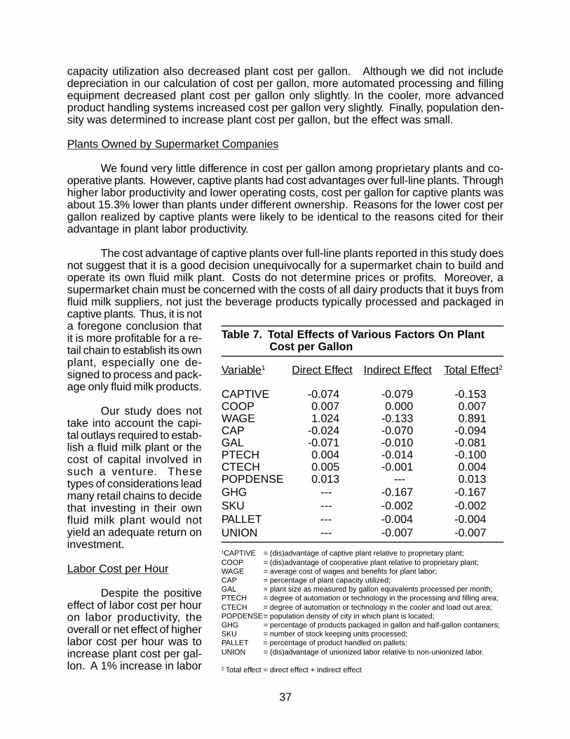
37
capacity utilization also decreased plant cost per gallon. Although we did not includedepreciation in our calculation of cost per gallon, more automated processing and fillingequipment decreased plant cost per gallon only slightly. In the cooler, more advancedproduct handling systems increased cost per gallon very slightly. Finally, population den-sity was determined to increase plant cost per gallon, but the effect was small.
Plants Owned by Supermarket Companies
We found very little difference in cost per gallon among proprietary plants and co-operative plants. However, captive plants had cost advantages over full-line plants. Throughhigher labor productivity and lower operating costs, cost per gallon for captive plants wasabout 15.3% lower than plants under different ownership. Reasons for the lower cost pergallon realized by captive plants were likely to be identical to the reasons cited for theiradvantage in plant labor productivity.
The cost advantage of captive plants over full-line plants reported in this study doesnot suggest that it is a good decision unequivocally for a supermarket chain to build andoperate its own fluid milk plant. Costs do not determine prices or profits. Moreover, asupermarket chain must be concerned with the costs of all dairy products that it buys fromfluid milk suppliers, not just the beverage products typically processed and packaged incaptive plants. Thus, it is nota foregone conclusion thatit is more profitable for a re-tail chain to establish its ownplant, especially one de-signed to process and pack-age only fluid milk products.
Our study does nottake into account the capi-tal outlays required to estab-lish a fluid milk plant or thecost of capital involved insuch a venture. Thesetypes of considerations leadmany retail chains to decidethat investing in their ownfluid milk plant would notyield an adequate return oninvestment.
Labor Cost per Hour
Despite the positiveeffect of labor cost per houron labor productivity, theoverall or net effect of higherlabor cost per hour was toincrease plant cost per gal-lon. A 1% increase in labor
Table 7. Total Effects of Various Factors On PlantCost per Gallon
Variable1 Direct Effect Indirect Effect Total Effect2
CAPTIVE -0.074 -0.079 -0.153COOP 0.007 0.000 0.007WAGE 1.024 -0.133 0.891CAP -0.024 -0.070 -0.094GAL -0.071 -0.010 -0.081PTECH 0.004 -0.014 -0.100CTECH 0.005 -0.001 0.004POPDENSE 0.013 --- 0.013GHG --- -0.167 -0.167SKU --- -0.002 -0.002PALLET --- -0.004 -0.004UNION --- -0.007 -0.007
1CAPTIVE = (dis)advantage of captive plant relative to proprietary plant;COOP = (dis)advantage of cooperative plant relative to proprietary plant;WAGE = average cost of wages and benefits for plant labor;CAP = percentage of plant capacity utilized;GAL = plant size as measured by gallon equivalents processed per month;PTECH = degree of automation or technology in the processing and filling area;CTECH = degree of automation or technology in the cooler and load out area;POPDENSE= population density of city in which plant is located;GHG = percentage of products packaged in gallon and half-gallon containers;SKU = number of stock keeping units processed;PALLET = percentage of product handled on pallets;UNION = (dis)advantage of unionized labor relative to non-unionized labor.
2 Total effect = direct effect + indirect effect

38
cost per hour, e. g., increasing from $20.60 per hour to $20.81 per hour in the averageplant, increased plant cost per gallon by 0.89%. This reflected labor’s overwhelming con-tribution to plant cost per gallon. On average, cost of labor accounted for about 67% ofnon-ingredient cost per gallon, excluding depreciation. The effect of hiring labor at 1%over the average labor cost per hour was to increase plant cost by 0.16¢ per gallon for theaverage plant.
Plant Size and Plant Capacity Utilization
Larger plant size and higher plant capacity utilization were earlier shown to in-crease plant labor productivity. Furthermore, we hypothesized that both factors also di-rectly impacted plant cost per gallon. The total effect of operating a larger plant, consider-ing both the direct effect on cost per gallon and the indirect effect on costs through in-creased labor productivity, was substantial if plant size changed significantly. For ex-ample, increasing from 2 million gallons per month to 3 million gallons per month de-creased plant cost per gallon by 4.1%. Increasing from 3 million gallons per month to 4million gallons per month further decreased plant cost per gallon by 2.7%. Given ouranalysis was based on costs exclusive of depreciation, the cost advantage of larger plantswhen including depreciation is undoubtedly even larger because the investment per gal-lon is lower in larger plants.
The total effect on cost per gallon attributed to changes in percent plant capacityutilization was negative, but the effect was rather small. Earlier results showed that higherplant capacity utilization increased labor productivity, and we anticipated that the totaleffect of this factor would be a decrease in plant cost per gallon. The results in Table 7supported this hypothesis, but the effect was relatively small unless large changes in plantcapacity utilization were made. Increasing plant utilization by 1% decreased plant costper gallon by 0.09%.
Level of Automation
We believed initially that plants with more modern equipment, especially in thecooler and load out area, would have significant savings in labor costs, utility costs, andrepair and maintenance costs. In our analysis of plant cost per gallon, we did not includethe cost of depreciation. By doing so, we hoped to avoid misleading results which mightindicate that newer and more advanced equipment was more costly than older and morefully depreciated equipment. However, our attempt to capture the effects of technology onplant cost per gallon was not as successful as we had hoped it would be. We found thatincreasing cooler and load out technology resulted in very small increases in cost pergallon. For example, increasing in cooler and load out technology from 4 to 6 increasedplant cost per gallon by 0.2% (a 50% increase in cooler score x 0.004 = 0.20). We alsofound that increasing processing and filling technology only slightly decreased cost pergallon. Specifically, increasing processing and filling technology from 4 to 6 decreasedplant cost per gallon by 0.5%.
Population Density
Several plants located in large cities mentioned problems that they thought wereunique to metropolitan areas. We tested this idea by including the number of inhabitantsper square mile for each plant in the study as a relevant variable to explain differences in

39
cost. The average population density was 5,300 people per square mile, but there wastremendous variation among the 35 plants. Plants in rural areas or small towns typicallyhad population densities of less than 1,000 people per square mile, but plants in largemetropolitan areas had population densities 8 to 10 times higher. In the most extremecases, population density averaged 33,400 people per square mile for the three plantslocated in the most urban settings.
Given the tremendous range in population densities, we expected to find a signifi-cant effect for population density. Specifically, we expected that plants located in moredensely populated cities would have higher costs per gallon than plants located in morerural settings. The results supported our hypothesis - plants located in large cities experi-enced higher costs per gallon. Specifically, a plant located in a city with 10,000 people persquare mile had plant costs 1.3% higher than a plant located in a city with 5,000 peopleper square mile.
Factors That Affect Cost Indirectly
We assumed that four factors affected plant cost per gallon only through their ef-fects on plant labor productivity. Specifically, we believed that unionized labor, containermix, number of SKUs processed, and percentage of product handled on pallets fell intothis category. Because these factors affected labor productivity, and labor productivityaffected plant cost per gallon, unionized labor, SKUs processed, container mix, and per-centage of product handled on pallets indirectly affected cost. To reflect this, we calcu-lated the impact of each of the four factors on plant cost per gallon (Table 7).
While the effects of any of these factors on cost per gallon were not insignificant,they were not extraordinary either. For example, unionized labor decreased cost pergallon by 0.7% through its effect on plant labor productivity. Similarly, increasing the per-centage of volume packaged in gallon and half-gallon containers by 10% (e. g., from 85%to 94%) decreased plant cost per gallon by 1.7%. The number of SKUs processed andthe percentage of volume handled on pallets impacted cost per gallon by less than 1% forcorresponding changes of less than 10%.
Comparing Regression and Neural Network Results
As with plant labor productivity, the plant cost data were analyzed using a neural net-work approach (12). The agreement between the two approaches was remarkably uniformdespite the dissimilar data analysis techniques used. For example, both analyses predictedcomparable decreases in cost per gallon for captive plant ownership, higher percentage ofplant capacity utilization, and higher percentage of product packaged in gallon and half-galloncontainers. A few of the results of the neural network approach differed slightly from thoseobtained using regression analysis in terms of the magnitude of the impact although the direc-tion of the impact was identical for both analyses. Percentage of plant volume handled onpallets, processing technology, SKUs processed, and plant size fell into this category. Theregression analysis predicted that unionized workforces would be slightly less costly on agallon basis than non-unionized workforces, that more advanced cooler technology increasecost per gallon very slightly, and that cooperative plants had costs per gallon about equal tothose of proprietary plants. The neural network approach predicted that unionized labor wouldbe significantly more costly than non-unionized labor, that more advanced cooler equipmentwould decrease cost per gallon very slightly, and that cost per gallon in cooperative plants was

40
higher than those of captive plants and proprietary plants. These incongruous results implythat the effects of unionization, cooler technology, and cooperative ownership on plant costper gallon were not determined conclusively by the two analyses.
We contend that the different results are largely related to the dissimilarities in dataanalyses encompassed by each technique. Specifically, we attribute the differences inour results to differences in model specification, presence of interaction terms, and func-tional form.
SECTION III: CHARACTERISTICS OF FLUID MILKDISTRIBUTION OPERATIONS
Types of Wholesale Routes
A distribution system for a fluid milk plant is complicated and unique to a particularplant. Even plants with similar physical characteristics and product mixes can have vastlydifferent types of customers and methods of distributing their products. Wholesale routescan be categorized by the types of customers served and include branch/depot routes,dealer routes, company operated routes and other specialty routes.
The delivery point of a branch/depot route is a distribution center where the deliv-ered product can be “cross-docked” to other delivery vehicles or temporarily held in thedistribution center. Although the branch/depot may be owned and operated by the milkplant itself, it need not be. A warehouse operation is an example of branch or depot whichmay be owned and operated by an organization other than the milk plant.
A dealer route is loaded by milk plant personnel, but the actual route is owned andoperated by an independent distributor. The product is purchased F. O. B. the plant dock,and the independent distributor incurs all expenses of delivering the product to customers.
Most of the products stored in the coolers of the participating plants were distrib-uted by company operated routes. As such, the milk company operated (or contractedwith) a distribution fleet that serviced customers with direct store deliveries (DSD). Theexact delivery agreement may vary, but a customer’s order was typically delivered to thecustomer’s dock or placed in the customer’s cooler.
Company operated routes can be broken down further into regular mixed routesand specialized routes. Mixed routes, sometimes called “peddle routes”, differ from spe-cialized routes by the types of customer served and the number of stops per day made byeach route delivery vehicle. A mixed route may be scheduled to make 15 to 30 stops perdelivery day and serves a wide variety of customers, including convenience stores, smallgrocery stores, restaurants, delis and, in some cases, a limited number of supermarkets.A specialized route is typically scheduled to serve 1 to 8 customers per delivery day andserves only large customers — supermarket stores, large convenience stores or clubstores (e. g., Price Club, Pace, Sam’s Club).
Figure 29 provides a graphical description of the average percent of plant volumedistributed on various types of wholesale routes by the participating plants. The volume ofproduct distributed through specialized routes dominated all other distribution categories,representing about 52% of all volume distributed.

41
With regular mixed routes accounting foranother 17%, about 70% of all product volumewas distributed through company operatedroutes serving customers directly from the plant.Branch/depot routes, which included ware-house deliveries, accounted for only about 11%of the total plant volume distributed, althoughseveral participants express interest in the pos-sibility of further developing these types ofroutes.
Other descriptors of wholesale routes in-cluded use of contract haulers, extent of directstore deliveries (DSD), and arrangements withcustomers concerning order deliveries. About55% of the plants maintained DSD with all oftheir wholesale accounts (Figure 30). About50% of the respondents indicated that they usedcontract haulers for at least one wholesaleroute, and they offered several reasons for con-tracting with independent haulers. The most common explanation was that the location ofcertain accounts was out of the standard delivery area covered by the plant. Anotherreason offered for using contract haulers was the lack of availability of backhaul materials(usually packaging) or products in outlying delivery areas. In other words, backhauls canoffset some of the costs of delivering to outlying areas, and if backhauls are not available,delivery costs may be lowered by contracting with independent haulers.
About 60% of the plants in the surveymaintained F. O. B. agreements with one ormore customers, but the actual percentage ofF. O. B. customers within a single plant tendedto be small.
Size of Wholesale Customers
Case size was variable among fluid milkplants, but all participating plants used 16–quart,20–quart, or 24–quart cases. Because overthree-fourths of all plants surveyed used 16–quart cases, we standardized case size in allplants to 16–quart equivalents. When catego-rized by the number of cases taken per deliv-ery, customers accepting over 100 cases perdelivery accounted for an average of 42% theof customers and 63% of the volume distributedby the plants (Figure 31). Not surprisingly, cus-tomers that receive small orders accounted fora very small percentage of the volume distrib-uted by the plants. For example, customers that
Bra
nch
Dea
ler
Mix
ed
Spe
cial
ized
Oth
er0
10
20
30
40
50
60
Per
cent
of
plan
t vo
lum
e
Bra
nch
Dea
ler
Mix
ed
Spe
cial
ized
Oth
er
Figure 29. Percent of plant volumedistributed by various methods
Figure 30. Miscellaneous distributioninformation
So
me
cont
ract
haul
ers
Som
e F
OB
do
ckde
liver
ies
100%
dire
ctst
ore
deliv
erie
s
0
10
20
30
40
50
60
70
80
90
100
Per
cent
of
plan
ts
So
me
cont
ract
haul
ers
Som
e F
OB
do
ckde
liver
ies
100%
dire
ctst
ore
deliv
erie
s
noyes

42
receive less than 5 cases per de-livery represented about 8% of allwholesale customers, but only ac-counted for an average of 1% ofthe volume distributed by eachplant’s wholesale routes. The twolargest customer categories (cus-tomers receiving more than 50cases per delivery) representedabout 53% of the customers andover three–fourths of the volumedistributed by plants. Many ofthese accounts would typically beserved by the specialized routes.
Cost of Delivery Implements
Summary statistics for re-ported replacement costs, offsets,and life expectancies for variousdelivery implements are presentedin Table 8. In general, most dairiesdid not require customers to con-tribute cost offsets (deposits) ondelivery equipment. Deposits werenot required for some deliveryequipment, such as handtrucksand pallets, but deposits were re-quired on some of the equipmentleft with the customers, such asbossie carts and plastic cases.
The most frequently usedproduct handling implements wereplastic cases and pallets. Plasticcases averaged about $2.03 eachwith a range of $1.58 to $2.70 percase, while cost of pallets averagedabout $9.37, and ranged from$3.80 to $15.00 per pallet. Abouthalf of the dairies in the study re-quired a deposit for plastic cases.The amount of the offset variedwidely among plants. The mini-mum reported case deposit was$0.25, and the maximum reporteddeposit was $2.00. None of thedairies required deposits for pallets.The life expectancy of a plastic
1 to
5
6 to
10
11 t
o 15
16 t
o 20
21 t
o 50
51 t
o 10
0
over
100
0
10
20
30
40
50
60
70
Pe
rce
nt
1 to
5
6 to
10
11 t
o 15
16 t
o 20
21 t
o 50
51 t
o 10
0
over
100
Number of cases per delivery
customersvolume
Figure 31. Size of wholesale deliveries by per-cent of customers and percent of plant volume
Table 8. Costs per Unit, Life Expectancies,and Deposits for Various Delivery Implements
LifeCost Expectancy Deposit
Plastic case:average $2.03 3.1 years $1.42low 1.58 1.0 0.25high 2.70 5.0 2.00median 2.00 3.0 2.00
Pallet:average $9.37 2.6 years $0low 3.80 0.5 0high 15.10 5.0 0median 7.75 2.0 0
Handtruck:average $135 4.4 years $0low 100 1.0 0high 215 15.0 0median 122 2.5 0
Bossie cart:average $530 6.7 years $483low 250 1.0 100high 754 20.0 750median 536 6.0 600
Dolly:average $52 4.6 years $0low 28 3.0 0high 70 8.0 0median 53 4.5 0

43
case, as measured by years of use, averaged 3.1 years. Some dairies in the Northeastreported life expectancies as trippage, i.e., the number of trips made before the case wasretired or missing. Under this type of evaluation, plastic cases averaged about 31 trips.The life expectancy for pallets averaged 2.6 years, and ranged from 6 months to 5 years.
Among the equipment commonly used during delivery, bossie carts were the mostcostly to replace, but they were expected to have the longest useful life of all deliveryequipment. The average replacement cost for a bossie cart was $530, and despite thehigh replacement cost, most dairies did not require a deposit on bossie carts. Bossie cartswere generally expected to last a minimum of five years, although a few dairies reportedlife expectancies of less than 3 years.
Description of Specialized Routes
A specialized or “supermarket” route typically serves 1 to 8 customers per deliveryday and serves only large customers — supermarket stores, large convenience stores orclub stores. Specialized routes are targeted in this study for two reasons. First, the costsof serving 15 to 30 individual customers on regular mixed or peddle routes vary widelybecause of the tremendous differences in the size of delivery taken by each customer anddifferences in levels of service. Consequently, an average delivery cost per case for regu-lar mixed routes is not meaningful for comparative purposes. Second, about 66% of milkpurchased for off-premise family consumption is sold through food chain stores, and su-permarket chains account for about 55% (13). The unit costs of serving customers onspecialized routes are generally considered similar across customers, and although ordersizes and service arrangements may differ between customers, the variation is not likelyto be highly significant. Furthermore, because of the large size of the deliveries, the percase fixed costs of serving each customer are small. Consequently, an average cost ofdelivery per case for specialized routes carries more meaning for comparative purposesthan its mixed route counterpart. The remainder of the discussion on distribution opera-tions concentrates exclusively on specialized routes.
Frequency of Delivery to Large Customers
On average, most of the large accountcustomers received shipments three or four daysa week (Figure 32). The combination of thesetwo categories totaled about two-thirds of alllarge accounts. About 20% of large account cus-tomers received deliveries five days a week, andanother 11% received deliveries six days perweek. Only about 3% received shipments twodays per week, and less than 1% received de-liveries 7 days per week. Although not indicatedby the barchart, there was substantial variationamong the participating plants. For example,several plants indicated that at least 80% of theirlarge accounts received deliveries three days perweek.
Figure 32. Weekly frequency ofdeliveries to large accounts
2 3 4 5 60
10
20
30
40
50
Per
cent
of
deliv
erie
s
2 3 4 5 6
Deliveries per week

44
Delivery Methods for Large Accounts
The delivery methods most fre-quently used on specialized routes werepallets, bossies, drag stacks, andhandtrucks (Figure 33). Nearly 80% ofthe participants indicated that palletswere used when delivering orders tolarge customers. A single pallethandles a large volume of product —about 54 16–quart cases (216 gallonequivalents). Pallets are handled byforklifts or electric hand jacks and aregenerally reserved for accounts that ac-cept over 100 cases per delivery. About65% of the plants used bossie carts fordelivering product. Bossie carts areavailable in two sizes — 120 gallon unitsand 90 gallon units. The 90 gallon unitsare gaining acceptance because of theirincreased maneuverability over theirlarger counterparts. Bossie carts tend to be favored by retailers because of the ease ofproduct handling in their coolers. Although there were some exceptions, the volume ofproduct handled on bossie carts within a single plant tended to be small. However, cap-tive plants tended to use bossie carts, as well as pallets, as the sole means of handlingproduct on their specialized routes.
Roughly an equal percentage of plants reported using drag stacks and handtrucksto deliver orders to large accounts. The drag stacks method, which appears to be themost physically demanding of all delivery methods, involves dragging a stack of five or sixcases with a metal hook from the delivery vehicle to the customer’s dock or cooler. A littleover half of the respondents report using handtrucks to transfer product from the deliveryvehicle to the customer’s dock or cooler. As with drag stacks, handtrucks are limited tomoving one stack of cases at a time. Dollies and flat trucks are less frequently usedmethods for delivering product. About 31% of the plants used dollies, but as with bossiecarts, the actual percentage of volume handled on dollies within a single plant tended tobe small.
Type of Driver Compensation on Specialized Routes
Figures 34 and 35 provide a graphical summary of information on driver compen-sation plans for specialized route drivers. About 78% of the drivers were paid on an hourlybasis, and another 18% were paid on base/commission plans. Only about 4% of thedrivers were paid on a salary basis. Although the majority of drivers were paid hourly, onlyabout 65% of the dairies reported paying overtime to drivers (Figure 34). Nearly all partici-pating plants reported that only one person, the delivery vehicle driver, was typically re-quired to distribute product to customers (Figure 35). However, some plants indicated thata driver may be accompanied by a second person during the training period for a newly-hired routeman. Dairies reporting regular use of multiple route personnel indicated that a
Figure 33. Percent of plants using variousdelivery implements on specialized routes
palle
ts
boss
ies
dra
gst
acks
ha
nd
tru
ck
dolli
es
flat
truc
k
0
10
20
30
40
50
60
70
80
90
100
Per
cent
of
milk
pla
nts
palle
ts
boss
ies
dra
gst
acks
ha
nd
tru
ck
dolli
es
flat
truc
k
noyes

45
second person was needed for security reasons.
Delivery Vehicles for Specialized Routes
Because specialized routes serve customers who take large quantities of product,tractor-trailers were often used for deliveries. However, some plants with specialized routesmaintained some straight-chassis trucks in the delivery fleet to deliver orders to largeaccounts. Clearly, the size of the loads carried on various types of delivery vehicles varieswith the size of the truck or trailer (Figure 36). Working load sizes for straight chassistrucks were considerably smaller thanthose of trailers. Trucks carried about390 to 520 cases, depending on thelength of the truck. Trailers of length 28–to 35–feet carried an average load sizeof 855 cases. There was little reporteddifference between 40– to 43–foot trail-ers and 44– to 50– foot trailers in termsof working case capacity. Trailers oflength 40– to 43–feet carried an aver-age of 1,100 cases per load, and 44– to50–foot trailers averaged 1,150 casesper load. Although some companies re-ported a carrying capacity of 1,300 casesor more for 45–foot trailers, there wassome reported concern over road weightlimits. The most common delivery ve-hicle on specialized routes for most ofthe plants in the study was the 45–foottrailer. About two-thirds of the compa-nies reported using 45–foot trailers insome delivery capacity. Furthermore,
Figure 34. Methods of driverpayment on specialized routes
Figure 35. Miscellaneous special-ized route drivery information
18 f
t. tr
uck
22-2
8 ft
.tr
uck
28-3
5 ft
.tr
aile
r
40-4
3 ft
.tr
aile
r
45-5
0 ft
.tr
aile
r
0
200
400
600
800
1000
1200
Num
ber
of c
ases
per
loa
d
18 f
t. tr
uck
22-2
8 ft
.tr
uck
28-3
5 ft
.tr
aile
r
40-4
3 ft
.tr
aile
r
45-5
0 ft
.tr
aile
r
Type and size of delivery vehicle*all capacities standardized to 16-quart cases
Figure 36. Working load size in cases forvehicles on specialized routes
Driverovertime
Multipleroute
personel
0102030405060708090
100
Per
cent
of
milk
pla
nts
Driverovertime
Multipleroute
personel
noyes
hourly commission salary0
10
20
30
40
50
60
70
80
Per
cent
of
milk
pla
nts
hourly commission salary

46
fourteen companies reported that 75% or more of their delivery fleet consists of 45–foottrailers. Another three companies used 48-foot or 50–foot trailers as the main deliveryvehicle on specialized routes.
Characteristics, Productivity and Costs of Specialized Routes
A total of 35 plants submitted information on their distribution operations. Not allplants returned complete surveys, and consequently, the calculations within this sectionwere based on data submitted by 20 operations. A great deal of variability in responseswas observed in many of the topics covered.
Within a single distribution operation, route data was variable. In order to reducethe data to more manageable figures, the data for all routes operated by one plant wereaveraged. For example, although the direct delivery cost per case varied from route toroute for a single plant, the boxplots only describe the average direct delivery cost for thatoperation.
The following section analyzes data collected on 270 specialized routes servinglarge customers submitted by 20 companies. Basic descriptive information, such as num-ber of cases delivered per month, number of customer stops per month, number of milestraveled per month and cost of driver labor per hour are covered. The section concludeswith a look at three cost and efficiency measures: driver labor productivity, cost of driverlabor per case, and direct delivery cost per case.
0
1
2
3
4
5
6
50
75
100
125
150
175
10
15
20
25
30
mean = 21,050median = 20,210
mean = 99median = 97
mean = 3,260median = 3,280
Cases delivered
per month
Number ofcustomer stops
per month
Number of milestravelled per
month
Figure 37 - Descriptors of Specialized Routes
thou
sand
s of
mile
s
cust
omer
sto
ps
mean = 21,050median = 20,210
mean = 99median = 97
mean = 3,260median = 3,280
S
S
S
S
SS
thou
sand
s of
cas
es

47
Number of Cases, Number of Stops and Miles Travelled
Figure 37 presents some basic descriptors of specialized routes. An average of21,050 cases was delivered per month (4,895 cases per week) on specialized routes witha median of 20,210 cases (4,700 cases per week). The number of cases delivered rangedfrom about 12,000 to more than 30,000 cases per month (2,790 to 9,300 cases per week).
During the course of delivering these cases of product, an average of 99 stops permonth (23 stops per week) were made on these specialized routes serving large accounts.The number of customer stops needed by each plant to serve all of its large accountsvaried widely, but after excluding the plants with an unusually high or low number of stops,most plants report between 80 and 135 customer stops per month on specialized routes(19 to 32 stops per week).
Figure 37 also reveals the range in the number of miles travelled each month onspecialized routes. The average number of miles travelled was surprisingly variable andranged from about 750 miles to about 5,360 miles per month (175 to 1,245 miles perweek). All plants averaged about 3,260 miles per month. Furthermore, the median wasabout 3,280 miles, indicating that the specialized routes of half of the plants travel morethan an average of 3,280 miles per month, and half travel fewer than an average of 3,280miles per month.
Driver Labor Productivity
The measure of labor productivity used for the delivery operations was the numberof cases of product delivered per hour of driver labor. Driver labor productivity was calcu-lated as the number of cases delivered per month on a specialized route divided by thenumber of hours worked per month by the driver(s). For each distribution operation, weaveraged driver labor productivity on specialized routes for which data was submitted togenerate one measure per operation. Figure 38 shows the dis-persion of driver labor productivity for the participating distribu-tion operations. On average, 111 cases were delivered per hourof driver labor, and driver labor productivity ranged from 67 casesper hour to 223 cases per hour. The large difference betweenthe mean and median indicated that a few highly productive dis-tribution operations were influencing the average driver labor pro-ductivity. In fact, while most operations delivered 70 to 120 casesper hour of driver labor, five operations delivered more than 150cases per hour of driver labor.
Cost of Driver Labor per Hour
Labor cost included driver wages and company contribu-tions to benefits packages. The average cost of driver labor onthe specialized routes serving large accounts was about $22.05per hour with a median of $21.30 per hour (Figure 39). The rangewas about $16.10 to over $27.50 per hour.
The most frequently selected benefits to which compa-nies contributed were FICA, workman’s compensation, unemploy-
Figure 38
case
s pe
r ho
ur
Cases deliveredper hour
50
75
100
125
150
175
200
225
S
mean = 111median = 99
S

48
ment, medical, vacation, pension and gifts. However, not all com-panies made contributions to all of these categories.
Cost of Labor per Case
The average cost of driver labor was 23.4¢ per case (Fig-ure 40). The lowest reported cost of driver labor was about 8.2¢per case, and the highest was about 42¢ per case. For eachdistribution operation, we averaged the cost of labor per case onall specialized routes to generate one measure per operation.
Direct Delivery Cost per Case
We used two cost components to determine direct deliv-ery cost per case for specialized routes — the cost of driver laborand the cost of operating the delivery vehicle. The cost of oper-ating a delivery vehicle included depreciation, lease payments,insurance, fuel, oil, tires, maintenance, repairs, garage costs, truckwashing expenses, registration fees, and highway taxes. Foreach distribution operation, we averaged total labor and vehiclecost per case on all specialized routes for which data was sub-mitted to generate one measure per operation. Direct deliverycost averaged 38.8¢ per case and ranged from 21.6¢ per case to54.1¢ per case (Figure 41). The median direct delivery cost was40.5¢ per case.
The cost of operating the deliveryvehicle contributed an average of 43%to direct deliver cost per case. Cost ofdriver labor contributed the remaining57%. However, vehicle operating costsranged from 21% to 53% of direct deliv-ery cost per case.
NOTE: Direct delivery cost percase only reflected the cost of servinglarge customers, such as supermarketsand club stores, on routes that largely usetractor-trailers for delivery. An averageof 5 customers per day were served onthese specialized routes. The cost percase of serving smaller customers suchas small convenience stores, Mom andPop stores, delis and restaurants is ex-pected to be much higher than the directdelivery cost reported here.
Direct deliverycost per case
mean = 38.8¢median = 40.5¢
20
30
40
50
60
Figure 41ce
nts
per
case
S
S
Figure 40
cent
s pe
r ca
se
mean = 23.4¢median = 22.3¢
7.5
15.0
22.5
30.0
37.5
45.0
Cost of Laborper case
S
S
mean = $22.05median = $21.30
Figure 39
Cost of driverlabor per hour
15.0
17.5
20.0
22.5
25.0
27.5
30.0
dolla
rs p
er h
our
S
S

49
SECTION IV: FACTORS CAUSING ROUTE LABOR PRODUCTIVITYAND COSTS TO VARY ON SPECIALIZED ROUTES
Overview
In the previous section, we reviewed general characteristics of the distribution op-erations of the plants in the study. In this section, we attempt to disentangle the effects ofvarious factors on route labor productivity and direct delivery cost per case. We usedregression analyses to quantify the impacts of each of the factors. We found that type ofplant ownership and cost of labor had the largest impacts on route labor productivity anddelivery cost per case.
Developing Measures to Test
We investigated three measures of efficiency that were consistent with the goalsand objectives of the project. They can be generally categorized as route labor efficiencyand route cost measures:
• Cases of products delivered per hour of driver labor• Cost of driver labor per delivered case• Cost of driver labor and vehicle operation per delivered case
Driver labor productivity, cost of driver labor per case, and direct delivery cost per casewere calculated from survey data to ensure that comparable cost and labor productivityfigures were analyzed.
Driver labor productivity (DPROD) was defined as the number of cases of pro-cessed and purchased products delivered per month, divided by the total hours logged bydrivers during the course of delivering the orders. We did not include the hours worked byany plant employees, including the load out area, personnel involved in sales, or generaland administrative personnel in the calculation of driver labor productivity.
Because the cost of labor contributed an average of nearly 60% to direct deliverycost, we investigated the effects of various factors on driver labor cost per case. Driverlabor cost per case (DRCOST) was defined as the monthly cost of wages and benefitsdivided by the number of cases delivered per month. We did not include the cost of anyplant employees, including the load out area, personnel involved in sales, or general andadministrative personnel in the calculation of driver labor cost per case.
As an extension of driver labor cost per case, we also analyzed the direct deliverycost per case. Direct delivery cost per case (DELCOST) was defined as the sum of thecost of driver labor (wages and benefits) and the cost of operating the delivery vehicledivided by the number of cases delivered. Vehicle operating costs included depreciation,lease payments, insurance, fuel, oil, tires, maintenance, repairs, garage costs, truck washingexpenses, registration fees, and highway taxes. We did not include the cost of plant labor,including the cost of load out labor, other plant costs, selling expenses, and general andadministrative expenses in the calculation of direct delivery cost.

50
Selecting the Independent Variables
A number of key factors tested were basic route descriptors, such as driver wagesand benefits cost per hour (DRWAGE), miles travelled per month (MILES), number ofcustomer stops per month (STOPS), percentage of product that was delivered to the cus-tomers’ dock as opposed to the customers’ cooler (DOCK), and the percentage of productdelivered on pallets (PALLET). We also identified routes operated by captive plants (CAP-TIVE) and distinguished them from routes operated by proprietary and cooperative com-panies. Differences in population densities may affect labor productivity. We hypoth-esized that more densely populated areas reduced driver labor productivity. We recog-nized that many plants operated routes which do not require deliveries within the city inwhich the plant is located. Nonetheless, we included population density (POPDENSE) asa factor affecting labor productivity. Finally, we were interested to see if unionized driverlabor (UNION) had any measureable effect on route labor productivity and costs.
Notes On Distribution Data
Data on specialized route labor were reported for 270 routes, submitted by 20 dair-ies. The analyses of driver labor productivity was based on this data set. Only 15 dairiessubmitted information on route labor and delivery vehicle costs, and consequently, theanalysis of direct delivery cost per case was based on only 180 routes.
Summary statistics for the independent variables are often helpful in providing ori-entation while analyzing the results of the analysis. Because we used two different datasets to complete the analyses, separate summary statistics are provided for each data set(Table 9 below and Table 13 on p. 57). Unlike the data used for the boxplots in theprevious section, the summary statistics presented in Tables 9 and 13 were calculatedfrom individual specialized routes; they are not averages for each operation.
Table 9. Summary Statistics for Various Factors Affecting Driver Labor Productivity andDriver Cost per Gallon1
Average AverageMeasures of Efficiency and Cost Mean Median Low 10% High 10%
Driver labor productivity (DPROD), cases/hr 108 97 52 216Cost of driver labor (DRCOST), ¢/case 16.8 15.0 10.1 47.8
Independent VariablesDriver labor cost (DRWAGE), $/hr 23.39 23.41 16.55 32.27Miles travelled (MILES), thousand/month 3.15 2.98 0.74 6.85Customer stops (STOPS), number/month 97 93 48 168Orders delivered on pallets (PALLETS), % 49.3 40.0 0.0 100.0Orders delivered to dock (DOCK), % 82.9 100.0 13.0 100.0Population density (POPDENSE), 1,000/sq. mile 4.60 1.01 0.50 22.50
1Reflects 270 specialized routes operated by 20 companies for which labor costs were reported.

51
The figures in the column labeled “Average High 10%” (“Average Low 10%”) rep-resent the average values of the highest 10% (lowest 10%) of the routes. High and lowaverages for each characteristic were computed independently. For example, the 10% ofthe routes that travelled the most miles were not necessarily the same 10% routes thathad the highest labor cost per hour, or any other category.
Model Specification
We developed three models that were consistent with the goals and objectives ofthe study. All equations were based on exponential regression models. In log-transforma-tion, the equation used to model route labor productivity was specified as:
ln ln ln ln ln
ln ln
DRPROD DRWAGE MILES STOP DOCK
PALLET CAPTIVE UNION POPDENSEit it it it it
it i i i it
= + + + ++ + + + +
β β β β ββ β β β ε
10 11 12 13 14
15 16 17 18
To model driver labor cost per case and direct delivery cost per case, we proposed thefollowing two models
ln ln lnDRCOST DRPROD POPDENSE CAPTIVE
UNIONit it it it
it it
= + + ++ +
β β β ββ υ
20 21 22 23
24
ln ln ln ln
ln ln
DELCOST DRPROD DRWAGE MILES
STOPS CAPTIVE POPDENSEjt jt jt jt
jt j j jt
= + + +
+ + + +
β β β β
β β β ν30 31 32 33
34 35 36
where i=1,....,270 routes, j=1,...,180 routes, t=1,...,12 months, and εit, υit, and νit were ran-dom disturbances.
Statistical Notes
As with the plant regression analyses, we treated the distribution data as paneldata, and as such we assumed the regression disturbances to be both heteroskedasticand autoregressive. To correct the data, we used identical transformation procedures asdescribed in Section II.
In order to use a recursive framework as specified for models [7] and [8] and mod-els [7] and [9], it was necessary to test whether the contemporaneous covariances werezero. We tested the two sets of equations to determine if our hypothesis of zero contem-poraneous covariances was correct. Because our test statistics (2.582, 1.641) were lessthan the critical value for a Chi-square distribution with 1 degree of freedom at the 5%level of significance (3.841), we could not reject the hypothesis that contemporaneouscovariances were zero. As a consequence, route labor productivity was a predeterminedvariable insofar as route labor cost per case and direct delivery cost per case were con-cerned. As such, the unilateral causal dependence specified for models [7] and [8] andmodels [7] and [9] allowed for the application of OLS to each equation separately and ledto unbiased and consistent estimates.
[7]
[8]
[9]

52
RESULTS OF THE ANALYSES
Route Labor Productivity
Overview of Results
Route labor productivity on the 270 specialized routes averaged 108 cases deliv-ered per hour of driver labor and ranged from about 52 cases per hour on the top 10% ofthe routes to about 216 cases per hour on the bottom 10% of the routes. The resultssupported what seems intuitive about driver labor productivity (Table 10). Type of owner-ship had the largest effect with routes operated by captive plants outperforming routesoperated by cooperative and proprietary plants. Hiring labor at a higher cost and increas-ing the volume of product handled on pallets increased driver labor productivity. Routeswith higher mileage were found to have lower driver labor productivity. Although we hadanticipated that population density would decrease driver labor productivity, the resultsindicated that plants located in more densely cities realized significant gains in driver laborproductivity. Larger volumes of product delivered to the customers’ dock (as opposed tothe cooler) and larger number of stops per month were not significant variables affectingroute labor productivity. Route labor productivity for operations that employed unionizeddrivers was not significantly different from that on routes that used non-unionized labor.
Routes Operated by Captive Plants
Captive plants realized significantly higher driver labor productivity than routes op-erated by full-line dairies. Routemen of captive plants delivered 23.7% more cases perhour than those of coopera-tive or proprietary plants. Thiseffect was net of the other rel-evant variables and ac-counted for differences in la-bor cost per hour, percentageof product handled on pallets,route mileage, and number ofcustomer stops. On average,this amounted to about 26cases per hour.
What might explain thehigher routeman labor pro-ductivity on routes operatedby captive plants? Becausesupermarket personnel androutemen work for the sameorganization, scheduling andcoordination of deliveries arelikely to be better than that ex-perienced on other routes.Furthermore, routemen aremore likely to receive assis-tance from store personnel
Table 10. Regression Results for Route LaborProductivity 1
Variable2 Coefficient SE Probability
Constant -0.215 0.122 0.0786CAPTIVE 0.237 0.059 <0.0001UNION -0.049 0.367 0.8946DRWAGE 0.892 0.178 <0.0001MILES -0.136 0.038 0.0004STOPS -0.075 0.077 0.3275PALLET 0.047 0.025 0.0589DOCK 0.120 0.136 0.3787POPDENSE 0.403 0.034 <0.0001
1The R2 for the untransformed data was 74.1%, and the R2 for the transformed data was 98.2%.
2CAPTIVE = (dis)advantage of captive plant relative to full-line plants;UNION = (dis)advantage of unionized labor relative to non-unionized labor;DRWAGE = average cost of wages and benefits for routemen;MILES = number of miles travelled per month;STOPS = number of customer stops made per month;PALLET = percentage of orders handled on pallets;DOCK = percentage of orders delivered to customer's dock;POPDENSE= inhabitants per square mile of city in which plant is located.

53
during the course of delivery. Finally, deliveries from captive plants to their supermarketsmay also get priority when unloading. For example, if several delivery vehicles are waitingto unload, the supermarket may give its own trucks the privilege of moving to the front ofthe line. Although we have attempted to provide some insight to the result, there may beother reasons to account for the higher labor productivity on routes operated by captiveplants.
Labor Cost per Hour
Labor cost, including benefits, averaged $23.39 per hour, and Table 9 indicatedthat there were substantial differences in route labor compensation. The regression re-sults presented in Table 10 also indicated that differences in route labor productivity wereattributable to differences in labor cost. For example, plants hiring labor at 1% over theaverage had 0.89% higher labor productivity than plants hiring labor at the average cost.A 0.89% increase in labor productivity amounted to an increase of about 1 case per hour.
Miles Traveled
Specialized routes covered an average of 3,150 miles per month. However, about10% of the routes covered less than 1,000 miles per month, and about 14% covered morethan 6,000 miles per month. With the tremendous differences in miles traveled, we be-lieved this factor would have significant implications for driver labor productivity. Althoughthe results supported our hypothesis, the effect of miles traveled on driver labor productiv-ity was not enormous. Increasing route mileage by 1% decreased route labor productivityby 0.14%. These results indicated that labor productivity is not greatly affected unlessvery large changes in mileage occur.
Number of Customer Stops
Each stop on a route requires tasks that are independent of the size of the orderdelivered. These include decelerating and stopping the vehicle, waiting to unload, back-ing the tractor–trailer unit to the dock, meeting with store personnel to record the delivery,and retrieving empty cases, bossie carts, or pallets, secure trailer doors, and exiting thedelivery area. We believed that the time required to complete these “fixed” tasks wouldaccrue for a route with a large number of stops and would subsequently impact driverlabor productivity. Again, the results showed that the number of stops decreased driverlabor productivity, but the effect was not statistically significant.
Product on Pallets
Specialized routes typically serve customers that take 50 or more cases per deliv-ery. The large order sizes seem well-suited for pallets which can handle 54 16-quartcases. About 39% of the routes did not use pallets to handle products. On the other hand,about 41% of the routes handled 100% of the products delivered on pallets. The percent-age of product handled on pallets for the remaining 20% of the routes ranged from 20% to75%. A higher percentage of products handled on pallets would seem to suggest signifi-cant savings in the time required to move product from the trailer to the customers’ docksor coolers. However, we found that for a 1% increase in the percentage of product handledon pallets, driver labor productivity increased by only 0.047%.

54
The very minor effect of pallets on route labor productivity prompted us to speakwith industry executives about the use of pallets. We found that although using palletswas expected to require less physical effort on the part of the routeman, the time savingsassociated with pallets was expected to be small. In particular, a significant amount oftime may be expended searching for or waiting for a pallet jack to unload the delivery,reducing any time savings imparted by moving a large amount of product on a singlepallet.
Dock Deliveries
The percent of product that was delivered to the customers’ dock ranged from 13%to 100% with an average of 82.9%. Although some variation was evident, most routesdeliver to the customers’ dock. As with use of pallets, dock-deliveries tended to be all–or–none. In other words, the percentage of dock-delivered product for any specific route wasusually 0% or 100%. We hypothesized that a higher percentage of dock–deliveries wouldincrease driver labor productivity because placing orders in the cooler increases the timeneeded to complete a delivery. Although the results indicated that dock deliveries in-crease driver labor productivity, the effect was not statistically significant.
Population Density
We had hypothesized that more populated areas would decrease route labor pro-ductivity. Our reasoning was that congestion in the cities would slow drivers traveling fromcustomer to customer. However, the results revealed that the opposite is true — thehigher the population density of the city in which the plant was located, the higher theproductivity of the driver. For example, a routeman operating in a city with populationdensity 10% higher than the average delivered 4.0% more cases per hour. While it maybe tempting to attribute the advantage to fewer miles travelled, it would be incorrect. Wehave accounted for differences in miles travelled, number of customer stops, and so forth.
We offer two alternative explanations for the advantage in route labor productivityfor plants located in densely populated areas. First, customers located near the plant mayaccept larger order sizes than customers located further from the plant and in less denselypopulated areas. Second, population density may serve as a proxy for time of delivery.With increased traffic congestion in more densely populated cities, deliveries may be sched-uled for times that are more favorable for travel, i. e., early morning or late evening.
Unionized Labor
Most of the routes for which we collected data employed unionized driver labor, butabout 15% of the routes did not use unionized driver labor. We theorized that differencesin labor productivity attributable to unionized/non–unionized labor would be evident. How-ever, we did not find any difference in labor productivity among the routes with and withoutunionized labor. There was no statistical evidence to suggest that unionized labor wasmore productive or less productive than non–unionized labor after accounting for differ-ences in labor cost per hour, miles travelled per month, number of stops per month, per-centage of product handled on pallets, and so forth.

55
Driver Labor Cost per Case
Overview of Results
Driver labor cost per case was calculated as the total of routeman wages and ben-efits divided by the total number of cases delivered by the routeman. Driver labor cost percase on the 270 specialized routes averaged 16.8 ¢ per case and ranged from about10.1¢ per case to about 47.8¢ per case.
We assumed that two of the three factors that affected route labor productivity alsoimpacted driver labor cost per case directly. These factors were:
• type of ownership (i.e., route operated by captive plant or full-line plant )• population density of city in which plant is located
However, we also determined that four factors affected driver labor productivity only anddid not affect labor costs directly. These factors were:
• miles travelled• number of customer stops• percentage of product delivered on pallets• percentage of orders delivered to the customers’ dock
The results reported in Table 11 indicates only the direct effect of each factor. Table12 indicates the total effect of each variable. For those factors in the first bulleted list, thetotal effect included the indirect effect on driver labor cost (through changes in labor pro-ductivity) as well as the direct impact on cost. For the factors in the second bulleted list,the values presented describe only the indirect effect of each of the significant factors, asdetermined by the analysis of route labor productivity. Because of the method of derivingthe total effect of each variable on cost per gallon, no probabilistic statements can bemade.
The results supported what seems intuitive about driver labor cost per case (Tables11 and 12). Type of ownership had the most noticeable effect with routes operated bycaptive plants outperforming routes operated by cooperative and proprietary plants. Routesoperated by unionized drivers had higher labor cost per case than routes operated bynon–unionized drivers. By its effects on route labor productivity, higher mileage was foundto have higher driver labor cost per case, but the effect was small. Population density anduse of pallets decreased labor cost per case, but their effects were small as well.
Routes Operated by Captive Plants
Whether or not the route was operated by a captive plant had significant ramifica-tions for driver labor cost per case. Labor cost per case was 40.8% lower for captiveplants (Table 12). This effect was net of any other factors included in the model for driverlabor cost per case. For example, after accounting for differences in percentage of prod-uct handled on pallets, route mileage, and number of customer stops, driver labor cost percase on routes operated by captive plants was 41% lower than routes under differentownership. This amounted to a difference of about 6.8¢ per case.

56
Given the earlier re-sults which indicated thatroutes operated by captiveplants delivered more casesper hour of driver labor, weanticipated this result. How-ever, the effect of captive–owned routes was consider-ably larger than we expected.Closer analysis of this curi-ous result revealed that cap-tive plants tended to pay lessfor driver labor than propri-etary or cooperative plants.The combination of higherlabor productivity and lowerdriver labor cost per hourprobably explains, to somedegree, the low driver laborcost per case that captiveplants experienced.
Unionized Labor
Although we did notfind differences in route la-bor productivity attributableto the presence or absenceof unionized labor, we didfind differences in driver la-bor cost per case. Our re-sults indicated that routeswith unionized drivers hadhigher labor cost per casethan routes with non–union-ized drivers. Specifically, la-bor cost per case was about18% higher for routes with unionized drivers. This effect is net of differences in type ofroute ownership, miles travelled per month, percentage of product handled on pallets, andso forth. We suspected that the reason for the higher labor cost per case on routes withunionized drivers was directly related to higher labor cost per hour, which included wagesand benefits.
Population Density
We found earlier that the higher the population density of the city in which the plantwas located, the higher the productivity of the driver. Although this effect on productivitywas expected to decrease driver labor cost per case (indirectly), we were not certain thatthe total effect of population density would decrease driver labor cost per case.
Table 11. Regression Results for Driver Labor Costper Case 1
Variable2 Coefficient SE Probability
Constant 1.232 0.697 0.0783CAPTIVE -0.306 0.102 0.0031UNION 0.160 0.066 0.0019DRPROD -0.432 0.062 <0.0001POPDENSE 0.120 0.051 <0.0203
1The R2 for the untransformed data was 65.4%, and the R2 for the transformed data was 77.6%.2CAPTIVE = (dis)advantage of captive plant relative to full-line plants;UNION = (dis)advantage of unionized labor relative to non-unionized labor;DRPROD = number of cases delivered per hour of driver labor;POPDENSE= inhabitants per square mile of city in which plant is located.
Table 12. Total Effects of Various Factors On DriverLabor Cost per Case
Variable1 Direct Effect Indirect Effect Total Effect2
CAPTIVE -0.306 -0.102 -0.408UNION 0.160 0.021 0.181POPDENSE 0.120 -0.174 -0.054MILES --- 0.059 -0.059PALLET --- -0.020 -0.020
1CAPTIVE = (dis)advantage of captive plant relative to proprietary plant;UNION = (dis)advantage of unionized labor relative to non-unionized labor;POPDENSE= inhabitants per square mile of city in which plant is located;MILES = number of miles travelled per month;PALLET = percentage of orders handled on pallets.
2 Total effect = direct effect + indirect effect

57
As shown in Table 12, the total effect of population density served to decreasedriver labor cost per case, but the effect was relatively small. For example, a plant locatedin a city with population density 10% higher than the average in the sample had driverlabor cost that was 0.5% lower per case.
Variables That Affect Cost Indirectly
We determined that two factors affected labor cost per case only through theireffects on route labor productivity. Specifically, we believed that miles travelled and thepercentage of product delivered on pallets fell into this category. The indirect effect ofeach on driver labor cost per case is reported in Table 12.
The effects of the two factors on driver labor cost per case were not extraordinary.For example, increasing miles travelled by 1% over the average increased driver laborcost per case by 0.059%. The percentage of orders handled on pallets had even less ofan impact on driver labor cost per case.
Direct Delivery Cost per Case
Overview of Results
Only 15 dairies submitted information on route labor and delivery vehicle costs,and consequently, the analysis of direct delivery cost per case was based on 180 routes.Direct delivery cost was the sum of the cost of driver labor (wages and benefits) and thecost of operating the delivery vehicle. Vehicle operating costs included depreciation,lease payments, insurance, fuel, oil, tires, maintenance, repairs, garage costs, truck washingexpenses, registration fees, and highway taxes. We did not include the cost of plant labor,including the cost of load out labor, other plant costs, selling expenses, and general andadministrative expenses in the calculation of direct deliver cost.
Table 13. Summary Statistics for Factors Affecting Direct Delivery Cost per Case1
Average AverageMeasures of Efficiency and Cost Mean Median Low 10% High 10%
Direct delivery cost (DELCOST), ¢/case 36.8 34.4 17.3 63.1
Factors Used to Explain Variation
Driver labor productivity (DPROD), cases/hr 124 112 69 208Driver labor cost (DRWAGE), $/hr 22.62 23.07 16.83 34.24Miles travelled (MILES), thousand/month 3.19 2.98 0.70 7.11Customer stops (STOPS), number/month 98 95 47 179Orders delivered on pallets (PALLETS), % 62.5 100.0 0.0 100.0Orders delivered to dock (DOCK), % 81.9 100.0 18.2 100.0Population density (POPDENSE), 1,000/sq. mile 4.60 1.01 0.50 28.4
1Reflects 180 specialized routes operated by 15 companies for which labor costs and vehcile operating costs were reported.

58
Summary statistics for the influential factors are often helpful in providing orienta-tion while analyzing the results of the analysis. The summary statistics presented in Table13 were calculated from individual specialized routes and are not averages for each op-eration.
Direct delivery cost per case averaged 36.8¢ per case and ranged from about 17.3¢per case to about 63.1¢ per case on the 180 specialized routes for which both labor costsand vehicle operating costs were reported.
As we determined with driver labor cost per case, five factors found to affect driverlabor productivity also directly impacted direct delivery cost per case. Factors which affectlabor productivity (and thus impact delivery costs indirectly) and that also directly impactdelivery costs were:
• type of ownership (i.e., route operated by captive plant or full-line plant )• driver labor cost per hour• miles travelled• number of customer stops• population density
However, we also determined that two factors affected only driver labor productivity anddid not directly affect delivery costs. These were:
• percentage of product delivered on pallets• percentage of orders delivered to the customers’ dock
The results reported in Table 14 indicates only the direct effect of each factor. Table15 indicates the total effect of each variable. For those factors in the first bulleted list, thetotal effect included the in-direct effect on direct deliv-ery cost per case (throughchanges in labor productiv-ity) as well as the direct im-pact on delivery cost. Of thetwo variables in the secondbulleted list, only the per-centage of orders deliveredon pallets was found to besignificant, as determinedby the analysis of route la-bor productivity. Becauseof the method of derivingthe total effect of each vari-able on cost per gallon, noprobabilistic statements canbe made.
As we remarked ear-lier, we did not find differ-ences in driver labor pro-
Table 14. Regression Results for Direct DeliveryCost per Case 1
Variable2 Coefficient SE Probability
Constant 2.447 0.626 0.0001DRPROD -0.676 0.030 <0.0001CAPTIVE 0.112 0.036 <0.0022DRWAGE 0.892 0.178 <0.0001MILES 0.195 0.022 <0.0001STOPS 0.061 0.037 0.1036POPDENSE -0.048 0.012 <0.0001
1The R2 for the untransformed data was 83.8%, and the R2 for the transformed data was 99.5%.2CAPTIVE = (dis)advantage of captive plant relative to full-line plants;DRPROD = number of cases delivered per hour of driver labor;DRWAGE = average cost of wages and benefits for routemen;MILES = number of miles travelled per month;STOPS = number of customer stops made per month;POPDENSE= inhabitants per square mile of city in which plant is located.

59
ductivity attributable to thepresence or absence ofunionized labor, but we didfind differences in driver la-bor cost per case for routeswith unionized labor. Wesuspected that the reasonfor the higher labor cost percase on routes with union-ized drivers was directly re-lated to labor cost per hour,which includes wages andbenefits. For this reason,we did not include union-ized labor as a separatefactor for direct deliverycost per case.
The results sup-ported what seems intuitive about direct delivery cost per case (Tables 14 and 15). Routesoperated by captive plants had lower direct delivery costs per case relative to cooperativeand proprietary plants. Direct delivery cost per case was also higher for routes which paidmore per hour for driver labor. Routes with higher mileage and more customer stops werefound to have higher direct delivery cost per case. Plants located in cities with higherpopulation density had lower direct delivery costs per case. Percentage of product handledon pallets decreased direct delivery cost per case slightly, but its effect was small.
Routes Operated by Captive Plants
Given the results presented earlier, it was not unexpected that routes operated bycaptive plants had lower direct delivery costs per case. Specifically, we found that thedirect delivery cost per case of routes operated by captive plants was 27.2% lower thanroutes operated by proprietary or cooperative milk plants. This effect was net of any othervariables included in the model of direct delivery cost per case and amounted to about9.9¢ per case.
Perhaps the earlier results for driver labor productivity and labor cost per case forroutes owned by captive plants would suggest that the difference in direct delivery costper case for captive and non-captive routes would be even higher. However, closer analy-sis of the data revealed that vehicle costs for captive routes tended to be higher thanroutes operated by proprietary or cooperative plants.
What might explain the lower delivery cost on routes operated by captive plants?We would assert that the same factors that contribute to higher labor productivity on routesoperated by captive plants also contribute to lower direct delivery costs. Briefly, schedul-ing of deliveries are likely to be more coordinated than that experienced on other routesbecause supermarket personnel and routemen work for the same organization. Further-more, routemen are more likely to receive assistance from store personnel during thecourse of delivery. Finally, deliveries from captive plants to their supermarkets may alsoreceive top priority when unloading.
Table 15. Total Effects of Various Factors On DirectDelivery Cost per Case
Variable1 Direct Effect Indirect Effect Total Effect2
CAPTIVE -0.112 -0.160 -0.272DRWAGE 1.362 -0.603 0.759MILES 0.195 0.092 0.287STOPS 0.061 0.051 0.112POPDENSE -0.048 -0.272 -0.320PALLET --- -0.032 -0.032
1CAPTIVE = (dis)advantage of captive plant relative to proprietary plant;DRWAGE = average cost of wages and benefits for routemen;MILES = number of miles travelled per month;STOPS = number of customer stops made per month;POPDENSE= inhabitants per square mile of city in which plant is located;PALLET = percentage of orders handled on pallets.
2 Total effect = direct effect + indirect effect

60
Labor Cost per Hour
Differences in direct delivery cost per case were attributable to differences in laborcost. For example, plants hiring drivers at 1% more than the average had 0.76% higherdirect delivery cost per case than plants hiring labor at the average cost. This accounts forthe corresponding increase in route labor productivity.
Miles Traveled and Number of Customer Stops
Routes with high mileages and numerous customer stops were shown to decreaseroute labor productivity. We tested miles travelled and number of customer stops underthe presumption that both factors also affected costs directly. The total effect of eachfactor was significant (Table 15). For example, a 1% increase in miles travelled per monthincreased direct delivery cost by 0.29% per case. Similarly, a 1% increase in the numberof customer stops made per month increased direct delivery cost by 0.11% per case.
Population Density
One unexpected result presented earlier suggested that route labor productivitywas higher for plants located in densely populated areas. We speculated that deliverycosts would be affected directly by population density as well as the effect on driver laborproductivity. Our results indicated that plants located in more densely populated areashad lower direct delivery costs per case. For example, a plant located in a city with about4,650 inhabitants per square mile (1% more dense than the average for all plants) haddirect delivery costs that were 0.32% lower per case than the average plant.
SECTION V: SELLING EXPENSES ANDGENERAL AND ADMINISTRATIVE EXPENSES
Selling expenses and general and administrative (G & A) expenses were not in-cluded in calculations of plant costs or the distribution costs. These “overhead” expenseswere required to support both the plant and distribution operations and were not incurredto support only specialized routes.
In reporting these expenses, no attempt was made to allocate the selling expensesamong different types of routes, nor was any attempt made to allocate the G & A expensesbetween the plant and distribution operations. The selling expenses and G & A expensesare reported on the basis of total cost per gallon of all beverage product processed andpackaged in the plant. Thirty-five plants reported G & A expenses, and 25 plants reportedselling expenses. In general, captive plants did not report selling expenses.
Selling expenses included wages and benefits for distribution management, salesmanagement, route supervision foremen, sales representatives and order takers, adver-tising and promotion expenses and bad debt expenses. For G & A, expenses includedwages and benefits for office personnel, salaries and benefits for administrative person-nel, office overhead (electricity, depreciation, supples, dues data processing, communica-tions, contributions and public relations), interplant hauling fees, snow removal, security,legal fees, consulting fees and allocated corporate overhead.

61
Selling expenses and G & A expenses arepresented as costs per gallon of product processed(Figure 42). For the 25 plants reporting, sellingexpenses averaged 4.9¢ per gallon and rangedfrom less than 1¢ per gallon to over 12¢ per gal-lon. G & A expenses ranged from about 1¢ pergallon to about 13¢ per gallon and averaged about5.7¢ per gallon. Captive plants tended to havelower G & A expenses per gallon than full-line op-erations. The 8 captive plants averaged 4.1¢ pergallon, and the proprietary and cooperative plantsaveraged 6.2¢ per gallon.
Figure 42 - Selling and G & Acosts per gallon
mean = 4.9¢median = 3.7¢
mean = 5.7¢median = 4.3¢
Sellingexpenses
0
3
6
9
12
15
G & Aexpenses
cent
s pe
r ga
llon

62
REFERENCES
1 Angus, R.C. and G.E. Brandow. 1960. Changes in productivity in milk distribution in2 Pennsylvania markets, 1940-1957. Prog. Rpt. 221, Pennsylvania State Univ. Agric.Exp. Stn., University Park.
2 Aplin. R.D. 1991. Factors contributing to profitability in fluid milk processing anddistribution operations. Dairy Marketing Notes. No. 1 Dep. Agric. Econ., CornellUniv., Ithaca, NY.
3 Aplin, R.D. 1991. Cost competitiveness of New York Metro area for processing fluidmilk for distribution to New York Metro area customers. Mimeo, Dep. Agric. Econ.,Cornell Univ., Ithaca, NY.
4 Beattie, B.R. and C.R. Taylor. 1985. The Economics of Production. John Wiley andSons, New York, NY.
5 Babb, E.M. 1967. Effect of assembly, processing, and distribution cost on marketingfluid milk. No. 828, Purdue Univ. Agric. Exp. Stn., Lafayette, IN.
6 Blanchard, W.H., G.McBride, and A.L. Rippen. 1962. A cost analysis of fluid milkpackaging operations. Tech. Bull 285, Michigan State Univ. Agric. Exp. Stn., EastLansing.
7 Bond, G.C.. 1978. Costs of processing and delivering milk in New Jersey, 1976-1977. S. R. 53, Dep. Agric. Econ. Marketing. New Jersey Exp. Stn., Cook Coll.,Rutgers Univ., New Brunswick.
8 Criner, G.K., G.K. White, and S.C. Howick. Fluid milk processing cost analysis. J.Dairy Sci. 78:1181.
9 Devino, G.T. and R.D. Aplin. 1968. Measuring and improving the profitability of milkdistribution routes. Bull. 1015. Cornell Univ. Agric. Exp. Stn., Ithaca, NY.
10 Erba, E.M., R.D. Aplin, and M.W. Stephenson. 1996. An analysis of processing anddistribution in 16 fluid milk plants. Unpublished mimeo, Dept of Agric., Resource,and Managerial Econ., Cornell University, Ithaca, NY.
11 Erba, E.M. and A.M. Novakovic. 1995. The evolution of milk pricing and governmentintervention in milk markets. Ext. Bull. 95 - 05, Dept. of Agric., Resource, and Mana-gerial Econ., Cornell Univ., Ithaca, NY.
12 Erba, E.M., J.E. Pratt, R.D. Aplin, and M.W. Stephenson. 1996. Comparisons ofcosts and efficiencies between cooperative, proprietary, and captive fluid milk pro-cessors: a neural network approach. Res. Bull. 96 - 13, Dept. of Agric., Resource,and Managerial Econ., Cornell Univ., Ithaca, NY.
13 Federal Milk Order Statistics, March/April, 1993. FMOS - 394, United States Depart-ment of Agriculture, Division of Agricultural Marketing Services, Washington, DC.
14 Fischer, M., J. Hammond, and W. Hardie. 1979. Fluid milk processing and distribu-tion costs. Bull. 530, Univ. Minnesota Agric. Exp. Stn., Minneapolis.

63
15 Freeman, R.B. and J.L. Medoff. 1984. What Do Unions Do? Basic Books, Inc. NewYork, NY.
16 Gujarati, D.N. 1995. Basic Econometrics, 3rd Edition. McGraw-Hill Publ. Co., Inc.New York, NY.
17 Jacobs, S.L. and G.K Criner. 1990. Milk processing and distribution costs: theMaine model. Tech. Bull. 140, Univ. Maine Agric. Exp. Stn., Orono.
18 Jones, W. and F. Lasley. 1980. Milk processor sales, costs, and margins. USDA/Econ., Statistics, and Cooperatives Serv., 77. USDA, Washington, DC.
19 Jones, W.W. 1979. Milk processor - distributors’ sales, costs, and margins. Econ.Res. Serv., 66. USDA, Washington, DC.
20 Judge, G.G., R.C. Hill, W.E. Griffiths, H. Lutkepohl, and T. C. Lee. 1988. Introductionto the Theory and Practice of Econometrics, Second Edition. John Wiley and Sons,New York, NY.
21 Kmenta, J. 1971. Elements of Econometrics. Macmillan Publ. Co., Inc., New York,NY.
22 Lau, L..J. 1986. “Functional forms in econometric model building” in Handbook ofEconomics, Volume 3. Z. Griliches and M. D. Intriligator, eds. Elsevier SciencesPublishers B. V., Amsterdam, the Netherlands.
23 Metzger, H.B. 1979. Factors affecting the unit costs of milk distribution. Bull. 758,Agric. Exp. Stn., Univ. of Maine, Orono.
24 O’Connell, P. and W.E. Snyder. 1964. Cost of analysis of fluid milk processing anddistribution in Colorado. Tech. Bull. 86, Colorado State Univ. Exp. Stn., Fort Collins.
25 Pelsue, N.H., Jr. 1992. Milk processing and distribution costs and returns. Res.Rep. 65. Vermont Agric. Exp. Stn., Burlington.
26 Strain, J.R. and S.K. Christensen. 1960. Relationship between plant size and costof processing fluid milk in Oregon. Tech. Bull. 55, Oregon State Coll. Agric. Exp. Stn.,Corvallis.
27 Thraen, C.S., D.E. Hahn, and J. B. Roof. 1987. Processing costs, labor efficiency,and economies of size in cooperatively - owned fluid milk plants. J. Agric. Coop2:40.
28 Weimer, M.R. and D.P. Blayney. 1994. Landmarks in the U. S. dairy industry. USDA,Econ. Res. Serv., Agric. Information Bull. No. 694.
29 Wood, T.M., G. A. Benson, and R.H. Carawon. UHT fluid milk processing costs.1985. Econ. Rs. Rpt. No. 50, Dept. of Econ. and Business, N. C. State University.,Raleigh.

OTHER AGRICULTURAL, RESOURCE, AND MANAGERIAL ECONOMICSRESEARCH BULLETINS
ORDER NO. TITLE AUTHOR(S)
R.B. 96-15 An Ex Post Evaluation of Generic Egg J. Carlos ReberteAdvertising in the U.S. Todd M. Schmit
Harry M. Kaiser
R.B. 96-16 Identifying Consumer Characteristics Yasuhito WatanabeAssociated with Japanese Preferences Nobuhiro SuzukiTowards Milk Products Harry M. Kaiser
R.B. 96-17 Distribution of Community Water Systems Richard N. BoisvertAcross the United States with Emphasis Todd M. Schmiton Size, Water Production, Ownership,and Treatment
R.B. 96-18 Rural Utility Service's Water and Waste Todd M. SchmitDisposal Loan and Grant Program and its Richard N. BoisvertContribution to Small Public Water SystemImprovements in New York State
R.B. 96-19 A Theory of Nonprice Export Promotion with Henry W. KinnucanApplication to USDA's Subsidy Programs Hui Xiao
R.B. 96-20 Assessing the Effectiveness of MPP Meat Allison ComeauAdvertising and Promotion in the Japanese Ron C. MittelhammerMarket Thomas I. Wahl
R.B. 97-01 The Implications of Trade Liberalization for Phillip M. BishopFederal Milk Marketing Orders Andrew M. Novakovic
R.B. 97-02 Information Needs of Agricultural Exporters: Deborah StreeterResults from a Focus Group Series Nelson Bills
Jan Maestro–SchererRob Neenan
These publications should be requested from: Bonnie GloskeyPublications Office46 Warren HallCornell UniversityIthaca, NY 14853(607) 255-2102