an application of user segmentation and modelling at a

i

An Application of User Segmentation and

Predictive Modelling at a Telecom Company

Kevin Nigel Nazareth

Internship report presented as partial requirement for

obtaining the Master’s degree in Advanced Analytics

i

An Application of User Segmentation and Predictive Modelling at a Telecom Company

Kevin Nigel Nazareth MAA

2018

ii

NOVA Information Management School

Instituto Superior de Estatística e Gestão de Informação

Universidade Nova de Lisboa

AN APPLICATION OF USER SEGMENTATION AND PREDICTIVE

MODELLING AT A TELECOM COMPANY

by

Kevin Nigel Nazareth

Internship report presented as partial requirement for obtaining the Master’s degree in Advanced

Analytics

Supervisor: Ivo Gonçalves

Co‐Supervisor: Mauro Castelli

External Supervisor: Sabina Zejnilovic

iii

September 2018

DEDICATION

Dedicated to my parents for their unwavered love and support throughout my life.

iv

ACKNOWLEDGEMENTS

Firstly, I am grateful to the telecom company I was interning at for giving me the opportunity to work

with them on this project. It was an invaluable learning experience.

I owe a special thanks to my external supervisor and project lead, Sabina Zejnilovic, for advising and

mentoring me during the internship. Her expertise and guidance were the corner stone for the success

of the project, and the development of my skills in data science.

I would also like to thank my colleague and co‐worker, Susana Lavado, for being a model workmate

and friend. She was a pleasure to work with, and was always willing to share her knowledge, wit, and

code!

Finally, I am indebted to my Nova IMS advisors, Mauro Castelli and Ivo Gonçalves, for their time and

effort in reviewing my reports and ensuring I meet the requirements for completing this report and

the master program.

v

ABSTRACT

“The squeaky wheel gets the grease” is an American proverb used to convey the notion that only those

who speak up tend to be heard. This was believed to be the case at the telecom company I interned at

– they believed that while those who complain about an issue (in particular, an issue of no access to

the service) get their problem resolved, there are others who have an issue but do not complain about

it. The latter are likely to be dissatisfied customers, and must be identified. This report describes the

approach taken to address this problem using machine learning. Unsupervised learning was used to

segment the customer base into user profiles based on their viewing behaviour, to better understand

their needs; and supervised learning was used to develop a predictive model to identify customers

who have no access to the TV service, and to explore what factors (or combination of factors) are

indicative of this issue.

KEYWORDS

Supervised learning; machine learning; clustering; predictive models; unbalanced dataset; dimension

reduction

vi

INDEX

1. Introduction .................................................................................................................. 1

2. Chapter I: Literature Review ......................................................................................... 2

2.1. Machine Learning Algorithms ............................................................................... 2

2.2. Issue of High‐Dimensionality With Respect to Clustering ..................................... 2

2.3. Principal Component Analysis ............................................................................... 2

2.4. Clustering Methods ............................................................................................... 3

2.4.1. K‐Means .......................................................................................................... 3

2.4.2. K‐Means++ ...................................................................................................... 3

2.4.3. Partition around Medoids (PAM) ................................................................... 4

2.4.4. Clustering Large Application (CLARA) ............................................................. 4

2.5. Cluster Quality and Optimal Number of Clusters .................................................. 4

2.5.1. Elbow Curve .................................................................................................... 5

2.5.2. Average Silhouette Width .............................................................................. 5

2.5.3. Gap Statistic .................................................................................................... 6

2.6. Issue of Unbalanced Datasets ............................................................................... 6

2.6.1. Random Under‐Sampling (Downsampling) .................................................... 7

2.6.2. Synthetic Minority Over‐Sampling Technique (SMOTE) ................................ 7

2.7. Predictive Models .................................................................................................. 7

2.7.1. Decision Trees ................................................................................................ 7

2.7.2. Bayesian Generalized Linear Models (GLM) .................................................. 8

2.7.3. Ensemble Predictive Models .......................................................................... 9

2.8. Model Evaluation ................................................................................................. 13

2.8.1. Data Partitioning Methods ........................................................................... 13

2.8.2. Evaluation Metrics ........................................................................................ 13

3. Chapter II: Unsupervised Learning for User Segmentation ....................................... 16

3.1. Data ..................................................................................................................... 16

3.1.1. Data Sources ................................................................................................. 17

3.1.2. Applying PCA to High‐Dimensionality Data .................................................. 17

3.2. Choosing from Clustering Algorithm ................................................................... 18

3.2.1. K‐Means v/s CLARA ...................................................................................... 18

3.2.2. K‐Means v/s K‐Means++ ............................................................................... 20

3.3. Choosing the Optimal Number of Clusters ......................................................... 21

3.3.1. Elbow Curve .................................................................................................. 22

vii

3.3.2. Silhouette Plot .............................................................................................. 22

3.3.3. Gap Statistic .................................................................................................. 22

3.3.4. Conclusion .................................................................................................... 22

3.4. Clustering Results and Discussion ....................................................................... 23

4. Chapter III: Supervised Learning for Identifying Users with No Access ..................... 27

4.1. Data ..................................................................................................................... 27

4.1.1. Monitoring Systems ..................................................................................... 29

4.2. Interpretable Model (Decision Tree) ................................................................... 31

4.2.1. Interpretable Decision Tree from SMOTE Dataset ....................................... 32

4.2.2. Interpretable Decision Tree from Downsampling Dataset .......................... 32

4.3. “Blackbox” Predictive Models ............................................................................. 34

4.3.1. Tuning Parameters for the Predictive Models ............................................. 34

4.3.2. Comparison of Predictive Model Results ..................................................... 35

4.4. Predictive Model Results and Discussion ............................................................ 36

5. Conclusions ................................................................................................................. 38

6. Limitations and recommendations for future works ................................................. 39

7. Bibliography ................................................................................................................ 40

viii

LIST OF FIGURES

Figure 1: Example of an elbow curve ("K‐means Cluster Analysis", 2018) ................................ 5

Figure 2: Example of a silhouette plot ("K‐means Cluster Analysis", 2018) .............................. 5

Figure 3: Example of a gap statistic graph ("K‐means Cluster Analysis", 2018) ........................ 6

Figure 4: An example of a decision tree (Kulkarni, 2017) .......................................................... 8

Figure 5: Bagging and boosting ensembles (Quantdare, 2016) ................................................. 9

Figure 6: Illustration of random forest ensemble used for classification (Navlani, 2018) ...... 10

Figure 7: Difference between high and low learning rate (Donges, 2018) .............................. 11

Figure 8: Visualization of first 3 iterations of gradient boosting (Grover, 2017) ..................... 11

Figure 9: Visualization of gradient boosting after 20 iterations (Grover, 2017) ...................... 12

Figure 10: Visualization of gradient boosting after 50 iterations (overfitting) (Grover, 2017) 12

Figure 11: An example of data partioning for 5‐fold cross‐validation (Becker, n.d.) .............. 13

Figure 12: Example of a ROC curve (Srivastava, 2016) ............................................................ 15

Figure 13: Silhouette plot generated from K‐means clustering result with seed 1 ................. 19

Figure 14: Silhouette plot generated from CLARA clustering result with seed 1 .................... 19


Figure 16: Silhouette plot generated from CLARA clustering result with seed 2 .................... 19


Figure 18: Silhouette plot generated from K‐means++ clustering result with seed 2 ............. 20





Figure 23: Elbow curve generated from clustering results ...................................................... 22

Figure 24: Silhouette plot generated from clustering results .................................................. 22

Figure 25: Gap statistic graph generated for clustering results ............................................... 22

Figure 26: Bar chart of app usage per cluster .......................................................................... 23

Figure 27: Bar chart of TV usage per cluster ............................................................................ 23

Figure 28: Bar chart of premium content watched per cluster ............................................... 23

Figure 29: Bar chart of HD content watched per cluster ......................................................... 23

Figure 30: Pie chart illustrating the composition of the dataset by cluster ............................. 24

Figure 31: TV viewing habits on working days ......................................................................... 24

ix

Figure 32: TV viewing habits on non‐working days ................................................................. 25

Figure 33: Category of content watched by users of each cluster .......................................... 25

Figure 34: TV viewing behaviour by function type .................................................................. 26

Figure 35: Proportion of customers who complained about lack of TV access by cluster ...... 26

Figure 36: Plot of the percent of clients not online on Monitoring System 2 against the number

of minutes before complaint or service request (SR) ...................................................... 29

Figure 37: Plot of percent of clients not online on Monitoring System 1 against the number of

minutes before complaint ................................................................................................ 30

Figure 38: Percent of clients not online on either one of the monitoring systems against

number of minutes before complaint .............................................................................. 30

Figure 40: Interpretable decision tree explaining which variables lead to a service request

about the lack of TV access .............................................................................................. 33

x

LIST OF TABLES

Table 1: Example of a confusion matrix (Data School, 2014) .................................................. 14

Table 2: Evaluation metrics derived from a confusion matrix (Data School, 2014) ................ 14

Table 3: Data used for clustering ............................................................................................. 17

Table 4: Principal components, proportion of variance captured, and standard deviation ... 18

Table 5: List of clusters with their size and description ........................................................... 24

Table 6: List of input variables sourced for the predictive model ........................................... 29

Table 7: Confusion matrix of a decision tree generated from an unbalanced dataset ........... 31

Table 8: Confusion matrix of the results of a decision tree generated from a dataset balanced

using Downsampling ........................................................................................................ 31

Table 9: Confusion matrix of the results of a decision tree generated from a dataset balanced

using SMOTE ..................................................................................................................... 31

Table 10: Comparison of performance matrices of simple decision trees generated from

unbalanced, downsampled, and SMOTE datasets ........................................................... 32

Table 11: Tuning parameters tested for the GBM model ........................................................ 34

Table 12: Tuning parameters tested for the GBM model ........................................................ 35

Table 13: Comparison of the performance metrics of each predictive models ...................... 35

Table 14: Confusion matrix of GBM results on SMOTE dataset .............................................. 36

Table 15: Top 10 variables used by the GBM model ............................................................... 37

xi

LIST OF ABBREVIATIONS AND ACRONYMS

PCA Principal Component Analysis

PAM Partition around Medoids

CLARA Clustering Large Application

WSS Within‐cluster Sum of Squares

SMOTE Synthetic Minority Oversampling Technique

GLM Generalized Linear Model

GBM Gradient Boosting Machines

AUC Area under the Curve

ROC Receiver Operating Characteristic

TP True Positives

TN True Negatives

FP False Positives

FN False Negatives

1

1. INTRODUCTION

This report describes the work done during a 10‐month internship with a telecom company between September 2017 and June 2018. The project had two primary objectives: to profile TV customers’ viewing behaviour, and to try to identify customers who have no access to the TV service. This was part of a broader initiative by the company to improve the quality of its service, curtail customer dissatisfaction, and reduce churn.

The project objectives were exploratory in nature, and required the use of machine learning algorithms to detect patterns in the large volumes of data logged by in‐house monitoring systems. Unsupervised learning was to be used to segment TV usage data into sub‐groups (or clusters) based on similarities in their usage characteristics, and supervised learning was to be used to detect anomalies in the data that could identify customers who have no access to the TV service, and to explain what factors (or combination of factors) in the data are key indicators of a disruption in service.

Identifying customers who have an issue accessing the TV service was essential. It was the biggest issue customers complained about, and it was believed that a significant number of customers who have this issue with accessing the TV service do not complain about it. These customers were likely to be dissatisfied customers, and therefore needed to be identified. It was also important to understand the customer’s viewing behaviour in order to gauge how much of an impact the lack of access to the service could have on the customer at a given time.

This report is divided into three chapters. The first chapter is a brief literature review of the machine learning concepts, clustering and predictive modelling algorithms, and data science techniques that were implemented in the project. The second chapter outlines the approach used to apply clustering algorithms (unsupervised learning) to user segmentation, and describes the resulting user profiles that were formulated. The third chapter summarizes the process used to develop predictive models (based on supervised learning) for identifying customers who have no access to the TV service.

NOTE: The data used for this project was fully anonymized. All identifier variables were pre‐hashed and could not be used to trace usage data back to the customer. The data was used for the sole purpose of user segmentation and developing predictive models for identifying customers who have no access to the TV service.

2

2. CHAPTER I: LITERATURE REVIEW

2.1. MACHINE LEARNING ALGORITHMS

Machine learning algorithms are methods used by data scientists to discover patterns in big data that

lead to actionable insights. These algorithms can typically be classified into two groups: supervised and

unsupervised learning, based on the way they “learn” from the data. Supervised machine learning

algorithms require a pre‐existing dataset that has the correct values of the target variable that it needs

to predict. The algorithm then learns from this ‘training’ dataset, and can make predictions on new

data. Unsupervised machine learning algorithms learn to identify patterns in the data without a

specified target variable.

(Castle, n.d.)

Before data can be used by machine learning algorithms, it often requires pre‐processing to prevent

unstable or poor quality output. In the project, two issues were encountered during this pre‐processing

stage: an issue with high‐dimensional data in the dataset to be used for unsupervised learning, and an

issue with unbalanced data in the dataset to be used for supervised learning. These issues have been

described in sections 2.2 and 2.6 of this chapter.

2.2. ISSUE OF HIGH‐DIMENSIONALITY WITH RESPECT TO CLUSTERING

Problems with high dimensionality result from the fact that a fixed number of data points become

increasingly sparse as the dimensionality increases. For clustering purposes, the most relevant aspect

of the “curse of dimensionality” concerns the effect of increasing dimensionality on distance or

similarity. In particular, most clustering techniques depend critically on the measure of distance or

similarity, and require that the objects within clusters are, in general, closer to each other than to

objects in other clusters.

(Steinbach, Ertöz and Kumar, 2002)

One of the solutions to this issue is employing a dimension reduction technique that can reduce the

number of dimensions while maintaining sufficient richness in the data. One such technique, principal

component analysis, was adopted in the project.

2.3. PRINCIPAL COMPONENT ANALYSIS

Principal Component Analysis (PCA) is a dimension reduction technique that reads a table of

observations described by several inter‐correlated quantitative dependent variables, extracts the

important information from it, and represents the data in a set of new orthogonal variables called

principal components. The principal components capture the similarity of the observations and of the

variables as points in maps.

(Abdi & Williams, 2010)

Each principal component explains a proportion of the variance of the original dataset, and is

dependent on all its preceding components. Therefore, if n components are selected, it must be the

first n components. The number of principal components selected is usually less than the number of

original variables, as principal components are more data rich than the original variables.

3

Care needs to be taken when choosing the number of principal components to consider, to strike an

optimum balance between reducing the number of dimensions and preserving the richness and detail

in the data.

(Cliff, 1988)

2.4. CLUSTERING METHODS

Clustering is an unsupervised learning process that applies data mining and data analysis techniques

to segment data into groups based on their similarities. There are several clustering algorithms that

could have been explored, however due to time constraints, only three were considered in the project:

K‐Means, K‐Means++ and CLARA.

2.4.1. K‐Means

K‐Means is a popular clustering algorithms that works by grouping data points based on their proximity

to a centre (mean) point, forming hyper‐spherical clusters. It seeks to minimize the average distance

between points in the same cluster, usually using Euclidean distance.

(Trevino, 2018)

The advantage of K‐means is its speed, simplicity and ability to handle large datasets. However, its

drawbacks are that the number of clusters needs to pre‐specified, it is sensitive to outliers, it only

works with hyper‐spherical clusters, and its results can vary based on initialization.

2.4.2. K‐Means++

The standard K‐means method is based on random initialization of initial centre points, which may not

produce optimal clusters. K‐means produces a local optimum based on the initialization. K‐means++ is

a variant of the K‐means algorithm that mitigates (but not necessarily eliminates) this initialization

issue. The intuition behind it is that spreading out the initial cluster centres is a good thing. The first

cluster centre is chosen at random, and each subsequent cluster centre is chosen from the remaining

data points based on a probability proportional to its squared distance from the point’s closest existing

cluster centre.

The probability is defined by:

∑ ∈

Where:

D(x) is the distance to the closest existing cluster centre

(Arthur & Vassilvitskii, 2006)

4

2.4.3. Partition around Medoids (PAM)

The PAM algorithm (also referred to as the K‐medoids algorithm) is an alternative to the K‐means

algorithm. It works by finding a sequence of data points (called medoids) that are centrally located to

the clusters, and minimizing the sum of dissimilarities between the medoid and the other points

labelled to be in the cluster. PAM is more robust in the presence of noise and outliers because a medoid

is less influenced by outliers or extreme values compared to a mean. However, it is less

computationally efficient and is therefore better suited for small datasets.

(Van der Laan, Pollard & Bryan, 2003)

2.4.4. Clustering Large Application (CLARA)

CLARA is based on the PAM algorithm and is designed to deal with very large datasets. It works by first

getting a set of smaller samples of the actual data, and then using PAM to find medoids for each of the

samples. CLARA then returns its best output as the clustering result. If the samples are of an adequate

sample size and are randomly drawn, theoretically, they are expected to resemble the dataset.

(Kaufman & Rousseeuw, 2018)

2.5. CLUSTER QUALITY AND OPTIMAL NUMBER OF CLUSTERS

Cluster quality is a measure of cluster cohesiveness. A highly cohesive cluster is one in which its

members are more like each other than to members of a different cluster.

(Sileshi & Gamback, 2018)

All the clustering methods used for the project (k‐means, k‐means++, and CLARA) required the number

of clusters (k) to be pre‐specified.

Determining the optimal number of clusters for the dataset is a fundamental issue, because it is

somehow subjective and depends on the method used for measuring similarity, the parameters used

for partitioning, and the interpretability of the clustering results.

(Kassambara, 2017)

There are several methods that could be used to determine the optimal number of clusters (k),

however, only three methods were considered for the project: elbow curve, silhouette value and gap

statistic.

5

2.5.1. Elbow Curve

The elbow curve is a visual method to suggest an optimal

number of clusters for a dataset. It is a graphical

representation of the total within‐cluster sum of squares

(WSS), calculated for a range of values of ‘k’.

WSS is calculated using the following formula:

.

Where:

Xi is ith data point of the cluster

μk is the center of cluster Ck

WSS is the measure of compactness of the cluster. As ‘k’

increases, WSS decreases exponentially. The point at which the WSS starts to plateau is considered an

optimal number of clusters, as it indicates that adding an additional cluster wouldn’t improve the WSS

much. Visually, this looks like an elbow in the curve.

(UC Business Analytics R Programming Guide, n.d.)

2.5.2. Average Silhouette Width

The Silhouette width is a measure of cluster quality that

considers both tightness and separation. If i is a point in a

cluster, its silhouette width s(i) is calculated using the

following formula:

max ,

Where:

a(i) is the average distance between ‘i’ and all other

points of the cluster to which ‘i’ belongs

b(i) is the shortest distance between ‘i’ and a point

from its neighbour cluster

A silhouette width value lies in between ‐1 and 1. The higher

the value, the better the clustering. A value of 0 indicates that the point lies between two clusters. A

negative value indicates the point is assigned to the wrong cluster.

(Rousseeuw, 1987)

The average silhouette width over all points of a cluster is a measure of how tightly grouped all the

points in the cluster are. It can be calculated and compared, and the highest value would suggest the

optimal number of clusters for the data. Graphically, this would be the peak of the graph, as illustrated

in figure 2.

Figure 1: Example of an elbow curve ("K‐means Cluster Analysis", 2018)

Figure 2: Example of a silhouette plot ("K‐means Cluster Analysis", 2018)

6

2.5.3. Gap Statistic

The gap statistic is another method to determine the optimal

number of clusters (k). This is how it is calculated: If dii’ is the

Euclidean distance between two data points i and i’, then the

sum of pairwise distances for all points in the cluster r, can

be calculated as follows:

, ∈

The pooled within‐cluster sum of squares can then be

calculated for a range of values of k, as follows:

12

Where:

Dr is the sum of pairwise distances for all points in the cluster r

nr is the size of cluster r

The idea behind the gap statistic is to standardize the comparison of log (Wk) with a null reference

distribution of the data, i.e. a distribution with no obvious clustering. The estimate for the optimal

number of clustering is the value for which log (Wk) falls furthest away this reference curve ("Gap

Statistic", 2018). This calculation is contained in the following formula:

∗

Where:

Wk – the pooled within‐cluster sum of squares around the cluster mean

En* – denotes expectations under a sample of size n from the reference distribution

2.6. ISSUE OF UNBALANCED DATASETS

An unbalanced dataset is one in which the number of observations belonging to one class is

significantly lower than those belonging to other classes. A class that is poorly represented in the

dataset is called in minority class, while one well represented is called a majority class. Using an

unbalanced dataset for a predictive model can lead to bias and inaccuracy both for learning and

evaluation of the predictive model.

(Upasana, 2017)

There are many dataset balancing techniques that can be used to tackle this issue, however, only two

methods were considered for the project: random under‐sampling (Downsampling) and synthetic

minority over‐sampling technique (SMOTE).

Figure 3: Example of a gap statistic graph ("K‐means Cluster Analysis", 2018)

7

2.6.1. Random Under‐Sampling (Downsampling)

Random under sampling (or Downsampling) aims to balance the class distribution by

randomly selecting a subset of the observations from the majority class to match the number of

observations of the minority class. Downsampling typically produces a balanced dataset with all classes

equally represented. An advantage of this technique is that it does not replicate or synthetically create

any observations, which guarantees accuracy in the data. But the downside is that a lot of data from

the majority class is discarded in the process.

(Upasana, 2017)

2.6.2. Synthetic Minority Over‐Sampling Technique (SMOTE)

SMOTE works by introducing new observations to the training dataset that have are synthetically

fabricated to be similar to the existing observations in the minority class. An advantage of SMOTE is

that no observations from the majority class is discarded, however, fabricated data is introduced to

the dataset which is less reliable. SMOTE is particularly less effective for high‐dimensional data as there

is a greater risk of fabricating incorrect observations.

(Upasana, 2017)

2.7. PREDICTIVE MODELS

Predictive modelling is the process of using known results to develop and evaluate models to forecast

future outcomes. Predictive models are of two types: classification models and regression models.

Classification modelling is the task of approximating a mapping function from input variables to

discrete output variables (or classes) for a given observation. It requires that an observation be

classified into just one of two of more classes, e.g. determining if an email is “spam” or “not spam”.

Regression modelling is the task of approximating a mapping function from input variables to a

continuous output variable. The continuous output variable is an integer or floating point value, e.g.

predicting the selling price of a house.

(Brownlee, 2017)

There are numerous machine learning algorithms that can be used for predictive modelling, however,

due to time and resource constraints and specific business needs, only a few were explored for the

project. The predictive modelling algorithms explored were Decision Trees, Bayesian Generalized

Linear Model (GLM), Gradient Boosting Machines (GBM), and Random Forest.

2.7.1. Decision Trees

Decision trees are sequential models which logically combine a sequence of tests. Each test compares

a numeric attribute against a threshold value or a nominal attribute against a set of possible values.

(Kotsiantis, 2011)

8

The logical rules followed by a decision tree are intuitive and easy to interpret. An example of a decision

tree on whether or not to play golf, based on three factor variables ‐ outlook, humidity, and wind, is

shown in figure 4.

Decision trees can be pruned using many user‐defined parameters to meet a certain criteria or level

of interpretability, however, only three tuning parameters were used in the project:

1. Minimum split – the minimum number of values in a node that must exist before a split is

attempted.

2. Maximum depth – the maximum depth of the tree from the root node to a leaf. The root node

is considered to have a depth of 0.

3. Complexity – the parameter that determines whether or not a split improves the model fit.

Any split that increases the model fit by a factor greater than the defined complexity factor is

attempted.

(WebFOCUS, 2015)

2.7.2. Bayesian Generalized Linear Models (GLM)

Linear models are models that describe the relationship between target variable and predictor

variables as a linear function. Many estimation problems, such as the relationship between a person’s

height and weight, can be summarized by a simple linear equation. However, there are other

estimation problems whose variables and not linearly related, and conventional linear models cannot

be used for such problems. They also suffer from other limitations; they assume that the values of the

predictor variables are normally distributed, and the relationships between variables are continuous.

(StatSoft, 2004)

Generalized linear models (GLM), as the name suggests, generalizes a conventional linear model to be

used to predict responses both for dependant variables with non‐normal distributions and dependant

variables which are non‐linearly related to the predictor. However, they still suffer a drawback ‐ when

the dimension of the parameter space is large, strong regularization has to be used to fit the GLMs to

datasets of realistic size without overfitting.

(StatSoft, 2004)

Bayesian inference is a method for the regularization of GLMs. Very generally speaking, the Bayesian

approach to statistical inference differs from traditional inferences by assuming that the data are fixed

and model parameters are random. This sets up problems in the form of: what is the probability of a

hypothesis (or parameter), given the data at hand? Traditional inferences assume that the model

Figure 4: An example of a decision tree (Kulkarni, 2017)

9

parameters are fixed (though unknown) and the data are essentially random. These types of problems

can be stated in the general form: what is the probability of the data given a hypothesis?

(Starkweather, 2011)

2.7.3. Ensemble Predictive Models

Ensemble modelling refers to the technique of combining many weak independent predictive models

to get a more powerful predictive model. They help reduce noise, variance and bias, which are the

main weaknesses in independent models.

(Garg, 2018)

Ensemble modelling techniques can broadly be classified into two categories: bagging and boosting.

Bagging is a simple ensembling technique in which many independent predictors/models are built, and

then combined using some model averaging techniques (e.g. weighted average, majority vote or

normal average). The independent models are trained using a sub‐sample of the data where each

observation is chosen with replacement, so that each model is trained with different data. This results

in uncorrelated learners which in turn reduces variance and error of the ensemble. An example of a

bagging ensemble is the random forest model.

(Grover, 2017)

Boosting is an ensembling technique in which the predictors are built and connected sequentially

instead of being built independently. It employs the logic that the subsequent predictors learn from

the mistakes of the previous predictors. Unlike the bagging technique, observations are not chosen

based on random sampling with replacement, but based on error. Observations have an unequal

probability of appearing in subsequent models, and ones with the highest error appear most (since the

goal of the subsequent models is to reduce the error). Boosting models tend to overfit so tuning the

stopping criteria is essential. An example of a boosting ensemble is the gradient boosting model (GBM).

(Grover, 2017)

Figure 5: Bagging and boosting ensembles (Quantdare, 2016)

10

2.7.3.1. Random Forest

Random forest is an extension of the bagging ensembling techniques. It creates a bagging ensemble of

decision trees, but takes one extra step; in addition to taking a random subset of data, it also takes a

random selection of features to grow a collection of decision trees termed as a random forest. (Nagpal,

2017)

Random forest ensembles can be used for both regression and classification problems. In a regression

problem, the average of all the tree outputs is considered as the final output. In a classification

problem, the final output is typically based on a majority vote ‐ each tree votes and the most popular

class is chosen as the final output. An illustration of the working of a random forest ensemble algorithm

is shown in figure 6.

Figure 6: Illustration of random forest ensemble used for classification (Navlani, 2018)

Advantages of Random Forest:

It is highly accurate and robust

It is unlikely to overfit because it takes the average prediction of the individual trees

It can be used for both classification and regression problems

It automatically assesses relative feature importance and selection

It handles higher dimensional data very well

(Navlani, 2018)

Disadvantages of Random Forest:

It is computationally expensive to create a random forest model

It is more difficult to interpret compared to a single decision tree

(Navlani, 2018)

Tuning Parameters for Random Forest

There are many parameters that can be used to tune a Random Forest model, however, only two

parameters were used in the project:

1. Mtry – the number of variables randomly sampled as candidates at each split

2. Ntree – the number of decision trees to generate for the ensemble

(Breiman and Cutler, 2018)

11

2.7.3.2. Gradient Boosting Machines (GBM)

Gradient boosting machines are models that employ the boosting ensembling technique with the use

of gradient‐descent to minimize error in the ensemble. A GBM can be used for both regression and

classification problems.

(Natekin and Knoll, 2013)

Gradient Descent

Gradient‐descent is an optimization algorithm

that takes steps proportional to the negative of

the gradient of a cost (or error) function to its

local minimum. How big the steps are that

gradient‐decent takes into the direction of the

local minimum is determined by the so‐called

learning rate. The learning rate needs to be

optimized to find the local minimum in the least

amount of time. If the learning rate is too large,

it may not find the local minimum; if it is too

small, it may take too long to find the local minimum.

(Donges, 2018)

Visualization of gradient boosting

Below are a series of plots that visualize an example of the iterative learning process of gradient

boosting. The blue dots are the observations of input(x) and output(y) of the data, the red line shows

the prediction of the learner, and the green dots shows the residual (error) of the prediction.

Figure 8: Visualization of first 3 iterations of gradient boosting (Grover, 2017)

Figure 7: Difference between high and low learning rate (Donges, 2018)

12

Using the boosting technique, the algorithm reduces the error at each iteration. After 20 iterations,

the residuals are randomly distributed and close to 0, and the predictions are close to the true values,

as seen in figure below.

Figure 9: Visualization of gradient boosting after 20 iterations (Grover, 2017)

This is an optimal stopping point for the algorithm. If is allowed to continue, it gets starts to overfit the

training data (as shown in the figure below).

Figure 10: Visualization of gradient boosting after 50 iterations (overfitting) (Grover, 2017)

Advantages of GBM:

Provides very accurate predictions

Lots of flexibility – it has many tuning parameters to adjust and tweak the algorithm

Minimal data pre‐processing – it works great with both categorical and numerical variables


Disadvantages of GBM:

Prone to overfitting

Computationally expensive

Results are not very interpretable


13

Tuning Parameters for GBM

Many parameters can be used to tune a GBM model, however, only four parameters were used to

tune the GBM model in the project:

1. Interaction depth – the number of splits it has to perform on each tree in the ensemble

2. N.trees – the number of trees in the ensemble

3. Shrinkage – the learning rate of the GBM

4. N.minobsinnode – the minimum number of observations in the trees terminal nodes

(Bhalla, n.d.)

2.8. MODEL EVALUATION

Before a model is trained and evaluated, the dataset is first partitioned into two subsets, one for

training the model and the other to test the trained model using certain evaluation metrics. The data

partitioning methods and evaluation metrics used for the project are described below.

2.8.1. Data Partitioning Methods

2.8.1.1. Train‐Test split

A train‐test split is a single data split using a sampling method to produce two subsets: a train set and

a test set (for training and testing the model respectively). A train‐test split is fast to run and performs

well with large datasets. However, if the number of observations is small, there may be insufficient

data to train and test the model. Therefore, it is not suitable for small datasets.

(Becker, n.d.)

2.8.1.2. K‐fold Cross‐validation

Cross‐validation is an extension of the

train‐test split method. In cross‐

validation, the dataset is split into k

equal subsets, and the model process is

done k times ‐ each time using a

different subset for validation. Cross‐

validation is said to be more reliable, but

takes longer to run. It is particularly

advantageous when the dataset is small.

(Becker, n.d.)

2.8.2. Evaluation Metrics

Creating and developing predictive models is dependent on constructive feedback and evaluation

metrics, and improvements are made until a desirable result is reached. An important aspect of

evaluation metrics is their capacity to discriminate between model results. The choice of metrics is

dependent on the type of model, the data, and the reasons for developing the model.

(Srivastava, 2016)

Figure 11: An example of data partioning for 5‐fold cross‐validation (Becker, n.d.)

14

In the project, predictive models were evaluated primarily using the confusion matrix and metrics

derived from it.

Confusion Matrix

A confusion matrix is an evaluation metric for classification problems on test data where the true

values are known. It is an N x N matrix, where N is the number of classes being predicted.

An example of a confusion matrix for a binary classification

problem is shown in table 1. In this example, the number of

observations in the test set was 165, and had two possible

predictions – “yes” and “no”. Out of the 165 observations, the

model predicted “yes” 110 times and “no” 55 times (columns

of the matrix). In reality, 105 observations were “yes” and 70

observations were “no” (rows of the matrix).

Some of the evaluation metrics that can be calculated from a

confusion matrix for a binary classification problem are listed below.

Metric Formula Description

True positives (TP) Number of observations correctly predicted

as true

True negative (TN) Number of observations correctly predicted

as false

False positives (FP) Number of observations wrongly predicted

as true

False negatives (FN) Number of observations wrongly predicted

as false

Accuracy (TP + TN) / total How often the model got it right

Precision TP / (TP + FP) Proportion of positive cases that were

correctly identified

Recall / Sensitivity TP / (TP + FN) Proportion of actual positive cases that were


Specificity TN / (TN + FP) Proportion of actual negative cases that were


F1 Score 2TP / (2TP + FP + FN) Harmonic mean of precision and recall

Balanced Accuracy (Sensitivity + Specificity) / 2 Average of the sensitivity and specificity

Table 2: Evaluation metrics derived from a confusion matrix (Data School, 2014)

Table 1: Example of a confusion matrix (Data School, 2014)

15

Accuracy vs Balanced Accuracy

When it comes to unbalanced datasets with an underrepresented minority class, the accuracy measure

is highly biased, and the balanced accuracy is a better measure of performance. For example, consider

an imbalanced dataset that contains 98% “false” values and 2% “true” values, and the model output is

100% “false” values. This model would have an accuracy of 98%, which doesn’t accurately reflect the

performance of the model. On the other hand, the balanced accuracy of the model would be 50%

because the sensitivity of the model is zero. This is a better reflection of its poor performance.

Area under the ROC Curve (AUC – ROC)

The Receiver Operating Characteristic (ROC) curve is the plot of the false positive rate (1 – specificity)

and the true positive rate (sensitivity). It illustrates how much better a predictive model performs

compared to a random prediction. A model that predicts at chance will have a ROC curve that looks

like the diagonal. The further the curve is from the diagonal line, the better is the models predicting

ability.

(Grace‐Martin, n.d.)

The area under the curve is calculated to quantify the ROC curve to a single number. The figure below

illustrates an example of an ROC curve.

Figure 12: Example of a ROC curve (Srivastava, 2016)

16

3. CHAPTER II: UNSUPERVISED LEARNING FOR USER SEGMENTATION

User segmentation is the process of dividing the user base into segments based on their similarity, and

then profiling the segments based on their characteristics. User segmentation was used to profile the

TV users based on their viewing behaviour in order to better understand the users and their needs.

3.1. DATA

The data required for user segmentation was housed in two main data servers – SQL Server and

Hadoop cluster. This data included user profile data, equipment data, and program content data, and

minute‐to‐minute usage sessions data. The data was initially in the form of a log with a timestamp for

each entry every minute. In order to make this log data more manageable, the data was aggregated

by time periods – day time, prime time, and night time, and by working or non‐working days. The

features of the data such as TV equipment, program content, TV subscription, function (recording, live

TV), HD/SD, etc. were also extracted from multiple databases through the IDs contained in the log. The

features data was then transformed into percent values based on proportion of total watched, so that

the viewing behaviour can be better understood and compared with other users. The data was also

quantified by volume of usage, and frequency and standard deviation of usage based on number of

active time periods (usage of more than 15 minutes in the time period). These variables were left in

absolute values and not converted to percentages.

17

3.1.1. Data Sources

Source Type of data Filters

SQL server

User profiles

TV equipment

Program content

TV subscription

Filter for target audience – active TV users in the

month of February 2018.

SQL server Time dimension Time‐periods:

Day: 7:00 to 17:59

Prime: 18:00 to 11:59

Night: 00:00 to 6:59

Days:

Working day

Non‐working day

Hadoop cluster TV sessions data Filter for target date range and aggregate data from

minute granularity to the chosen time periods.

SQL server App sessions data Filter for target date range and aggregate data from

minute granularity to the chosen time periods.

Both app and TV sessions data were processed to

obtain the following features:

Time and volume of usage

Frequency of active time periods (more than

15 minutes of usage)

Standard deviation of active time periods

Device type – Phone, Tablet, TV, TV App

Service type – HD or SD

Category of program watched

Function type – live TV, video on‐demand,

recordings

Table 3: Data used for clustering

3.1.2. Applying PCA to High‐Dimensionality Data

The 71 dimensions in the dataset had to be reduced in order to mitigate the adverse effects of high‐

dimensionality mentioned previously in Section 2.3. Dimension reduction was done using principal

component analysis (PCA). The first 21 principal components are shown in the following table.

18

PC1 PC2 PC3 PC4 PC5 PC6 PC7

Standard Deviation 3.25 2.12 1.86 1.64 1.44 1.32 1.14

Proportion of Variance 0.26 0.11 0.09 0.07 0.05 0.04 0.03

Cumulative Proportion 0.26 0.38 0.46 0.53 0.58 0.63 0.66









Table 4: Principal components, proportion of variance captured, and standard deviation

In the table above, ‘Proportion of Variance’ refers to the amount of variance captured by the principal

component, and ‘Cumulative Proportion’ refers to the cumulative proportion of variance captured by

the principal component along with all its preceding components.

After trial‐and‐error, it was decided that 13 (PC13) would be an optimum number of principal

components to use as it captures more than 80% of the variance of the data and produced sufficiently

stable clustering results when run with different seeds.

3.2. CHOOSING FROM CLUSTERING ALGORITHM

The goal of the clustering algorithm was to produce meaningful and stable segments of the dataset.

To choose which clustering method best clustered the data, each was run with different seeds and the

results compared. Given that the dataset was large (800k users) and time and processing power were

limited, a 1% sample of the dataset was used, and silhouette plot was used as the cluster quality

measure. The number of clusters ‘k’ was tested for values from 2 to 10.

3.2.1. K‐Means v/s CLARA

K‐Means and CLARA algorithms were run on the 1% sample data, and the silhouette plots were

graphed for two seeds.

19

SEED = 1

Figure 13: Silhouette plot generated from K‐means clustering result with seed 1

Figure 14: Silhouette plot generated from CLARA clustering result with seed 1

SEED = 2


Figure 16: Silhouette plot generated from CLARA clustering result with seed 2

Analysis

The results of the CLARA algorithm were very unstable. For seed one, the silhouette scores ranged

from 0.1 to 0.2 but for seed two, it ranged from 0 to 0.7. The shapes of the silhouette plots were also

very dissimilar. Increasing the sample size within the CLARA algorithm did improve the stability of the

algorithm but could not match the stability of results from the k‐means algorithm. K‐means produced

silhouette values between 0.15 to 0.3 for both seeds, and the silhouette plots were also of similar

shape. Therefore, it was decided that K‐means was better than CLARA for the data because of its

stability on different seeds.

20

3.2.2. K‐Means v/s K‐Means++

Similar to the previous test, three 1% samples were taken from the dataset, and K‐means and K‐

means++ algorithms were applied to them. These were the resultant silhouette plots.

SEED = 1


Figure 18: Silhouette plot generated from K‐means++ clustering result with seed 2

SEED = 2



21

SEED = 3



Analysis

The difference between the silhouette plots of the three samples are minor. If the plots for seed 2 and

3 are compared, the K‐means++ plots are a tad more similar and therefore more stable. For this reason,

it was decided that the K‐means++ algorithm was preferred, and it became the algorithm of choice for

clustering the data.

3.3. CHOOSING THE OPTIMAL NUMBER OF CLUSTERS

As previously stated, one of the drawbacks of partition‐based clustering algorithms is the need to pre‐

specify the number of clusters ‘k’. Since K‐means++ was chosen as the preferred clustering method for

the data, it was the method used when determining the optimal number of clusters.

Clustering was done several times, with different data (all features, a combination of original features

and PCA, and only PCA), with different seeds and sample sizes of the dataset, and the final dataset

chosen was one with only PCA components and taking a 5% sample of the dataset. K‐means++

clustering was performed on this dataset for a range of values of k from 2 to 10. The results were then

analysed using the elbow curve, silhouette plot and gap statistic.

22

3.3.1. Elbow Curve

From the results of the k‐means++ clustering, the within‐

cluster sum of squares (WSS) was calculated for each value

of ‘k’ (2 through 10), and the resultant plot is shown in figure

23.

Analysis

The graph produced is a smooth curve with no clearly

identifiable elbow. This exercise was repeated with different

seeds but produced similar results. Therefore, the elbow

method did not clearly determine an optimal number of clusters for the dataset.

3.3.2. Silhouette Plot

The silhouette width was calculated and plotted for the

clustering results for each value of k, and resultant plot is

shown in figure 24.

Analysis

K = 3 (highest value of y) appeared to be optimal values of ‘k’

according to the silhouette plot. However, it would not give

rich enough clusters for the project needs, and so it was

ignored. The next peak was either k = 6, which was

sufficiently high to produce rich clusters, and therefore could

be considered as possible optimum number of clusters.

3.3.3. Gap Statistic

The gap statistic was calculated for the clustering results and

the resultant plot is shown in figure 25.

Analysis

The gap statistic showed 3 peaks, at k = 1, k = 6, and at k =

10. Peaks indicate the biggest ‘gap’ between the log (Wk)

value and the null reference distribution curve, which infer

optimal number of clusters for the dataset. Having a single

cluster means performing no clustering, which was not

acceptable. Therefore, the results of this gap statistic that

could be considered were either 6 or 10.

3.3.4. Conclusion

The elbow curve didn’t show an obvious elbow to suggest an optimum value of k, but both the

silhouette plot and the gap statistic suggested that 6 was a good number of clusters for the dataset,

but 7 was a close second. The clustering was performed on the entire dataset with both k = 6 and k =

7. After the results were analysed, it was decided that k = 6 produced more meaningful cluster (or user

segments). These user segments have been described in the “Clustering Results” section of the report.

Figure 23: Elbow curve generated from clustering results

Figure 24: Silhouette plot generated from clustering results

Figure 25: Gap statistic graph generated for clustering results

23

3.4. CLUSTERING RESULTS AND DISCUSSION

As previously stated, k‐means++ was the preferred clustering method, and k = 6 was chosen as the

optimum number of clusters for the data. After clustering of the entire dataset with these parameters,

the mean value for each dimension of each cluster was then calculated and compared. It was observed

that 5 of the 6 clusters had significantly different mean values for the app and TV usage dimensions,

which suggested that they were the main discriminating factor for the clustering. To reflect this fact,

the five clusters were named ‘Average TV’, ‘Light TV’, ‘Heavy TV’, ‘Light App’, and ‘Heavy App’.

The 6th cluster had a significantly high mean value for proportion of HD TV and premium content

watched, and the cluster was therefore named ‘HD TV’.

0,00 50,00 100,00 150,00 200,00 250,00

Average TV

Light TV

Heavy TV

HD TV

Light App

Heavy App

TV Usage for February (in hours)

0,00 20,00 40,00 60,00 80,00

Average TV

Light TV

Heavy TV

HD TV

Light App

Heavy App

App usage for February (in hours)

0% 10% 20% 30% 40%

Average TV

Light TV

Heavy TV

HD TV

Light App

Heavy App

Proportion of HD content watched

0,00% 5,00% 10,00% 15,00% 20,00% 25,00%

Average TV

Light TV

Heavy TV

HD TV

Light App

Heavy App

Premium Content Watched

Figure 27: Bar chart of TV usage per cluster Figure 26: Bar chart of app usage per cluster

Figure 29: Bar chart of HD content watched per cluster Figure 28: Bar chart of premium content watched per cluster

24

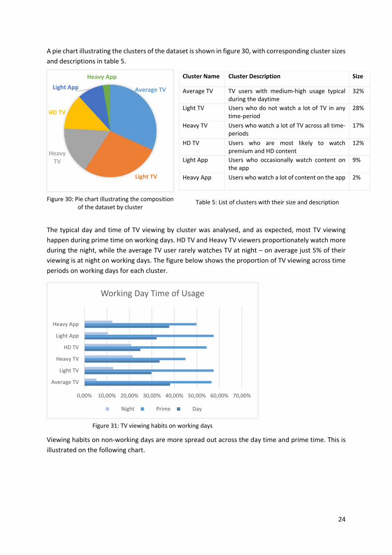
A pie chart illustrating the clusters of the dataset is shown in figure 30, with corresponding cluster sizes

and descriptions in table 5.

The typical day and time of TV viewing by cluster was analysed, and as expected, most TV viewing

happen during prime time on working days. HD TV and Heavy TV viewers proportionately watch more

during the night, while the average TV user rarely watches TV at night – on average just 5% of their

viewing is at night on working days. The figure below shows the proportion of TV viewing across time

periods on working days for each cluster.

Viewing habits on non‐working days are more spread out across the day time and prime time. This is

illustrated on the following chart.

Cluster Name Cluster Description Size

Average TV TV users with medium‐high usage typical during the daytime

32%

Light TV Users who do not watch a lot of TV in any time‐period

28%

Heavy TV Users who watch a lot of TV across all time‐periods

17%

HD TV Users who are most likely to watch premium and HD content

12%

Light App Users who occasionally watch content on the app

9%

Heavy App Users who watch a lot of content on the app 2%

Table 5: List of clusters with their size and description

Average TV

Light TV

Heavy TV

HD TV

Light App

Heavy App

0,00% 10,00% 20,00% 30,00% 40,00% 50,00% 60,00% 70,00%

Average TV

Light TV

Heavy TV

HD TV

Light App

Heavy App

Working Day Time of Usage

Night Prime Day

Figure 30: Pie chart illustrating the composition of the dataset by cluster

Figure 31: TV viewing habits on working days

25

Figure 32: TV viewing habits on non‐working days

The category of content watched by cluster was also analysed. It was observed that users most often

watch content categorized as ‘Entertainment’, followed by content categorized as ‘Info’ (which

includes news content). However, the exception is users of the ‘HD TV’ cluster – they most often watch

films and TV series. Figure 33 illustrates the proportion of content typically watched by users belonging

to different clusters.

Figure 33: Category of content watched by users of each cluster

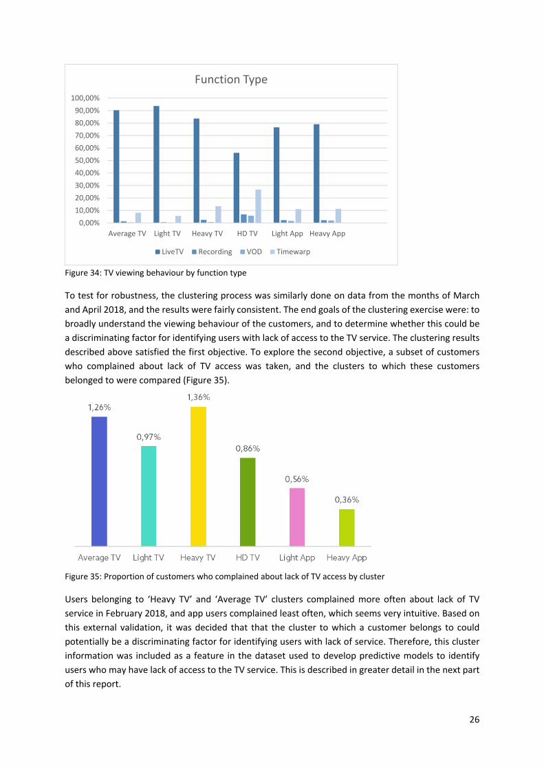
If the TV viewing behaviour is categorized in terms of function type, it was seen that most users watch

live TV, and occasionally use the ‘Timewarp’ feature to view missed live TV content (the company offers

its customers access to all content broadcasted in the last 7 days). Users belonging to the ‘HD TV’

cluster also tend use the ‘Recording’ function and the ‘VOD’ (Video‐on‐demand) function often. The

TV viewing behaviour by function for each cluster is illustrated in the following chart.

0,00% 10,00% 20,00% 30,00% 40,00% 50,00% 60,00%

Average TV

Light TV

Heavy TV

HD TV

Light App

Heavy App

Non‐working Day Time of Usage

Night Prime Day

0,00%

10,00%

20,00%

30,00%

40,00%

Average TV Light TV Heavy TV HD TV Light App Heavy App

Content Watched

Films Series Kids Sports Documentaries Entertainment Info

26

Figure 34: TV viewing behaviour by function type

To test for robustness, the clustering process was similarly done on data from the months of March

and April 2018, and the results were fairly consistent. The end goals of the clustering exercise were: to

broadly understand the viewing behaviour of the customers, and to determine whether this could be

a discriminating factor for identifying users with lack of access to the TV service. The clustering results

described above satisfied the first objective. To explore the second objective, a subset of customers

who complained about lack of TV access was taken, and the clusters to which these customers

belonged to were compared (Figure 35).

Figure 35: Proportion of customers who complained about lack of TV access by cluster

Users belonging to ‘Heavy TV’ and ‘Average TV’ clusters complained more often about lack of TV

service in February 2018, and app users complained least often, which seems very intuitive. Based on

this external validation, it was decided that that the cluster to which a customer belongs to could

potentially be a discriminating factor for identifying users with lack of service. Therefore, this cluster

information was included as a feature in the dataset used to develop predictive models to identify

users who may have lack of access to the TV service. This is described in greater detail in the next part

of this report.

0,00%

10,00%

20,00%

30,00%

40,00%

50,00%

60,00%

70,00%

80,00%

90,00%

100,00%

Average TV Light TV Heavy TV HD TV Light App Heavy App

Function Type

LiveTV Recording VOD Timewarp

27

4. CHAPTER III: SUPERVISED LEARNING FOR IDENTIFYING USERS WITH NO

ACCESS

The goal of the project was to identify users that do not have access to their TV service based on

features of the user profile and inputs from the in‐house monitoring systems. This was done using

supervised learning. Some users who don’t have access complain while others don’t. It is particularly

important for the company to identify the users who have no access but do not complain, because

these customers are most likely to be dissatisfied and most likely to churn.

4.1. DATA

The users who did complain were chosen as the target variable. Values from the monitoring systems

that monitor the TV service were taken at the hour of complain, one hour before, and two hours before

the complaint. In order to get data to explain what the normal values of the monitoring systems should

be, random samples of the population were gathered from two arbitrary days and times for all the

users who didn’t complain during the month of February 2018. The complaints dataset and the

population dataset were then combined to produce the final dataset. Here is an overview of the data

collected:

Population dataset (Negative class)

633,7 K users

Sample of data taken from four monitoring systems on an arbitrary hour during:

a) February 2, 2018. 17h‐19h

b) February 14, 2018. 12h‐15h

Complaint dataset (Positive class)

5,9 K users with SR of type “no access” for TV in the month of February 2018

Month analysed

February 2018

Time band

3 hours (16h00 ‐ 19h00) on February 2nd (weekday)

3 hours (12h00 ‐ 15h00) on February 14th (weekday)

Group of

variables

Subgroup of

variables Exploratory variables Observations

Technical signs Monitoring

System 1

Status of the Set Top Box (STB) Variables analysed for 3

different times:

a) hour of complaint;

b) 1 hour before

complaint;

c) 2 hours before

complaint

Volume of data uploaded by the

STB

Volume of data downloaded by

the STB

Signal Power STB is getting

Signal Power the STB is getting

28

Signal Power the STB is sending:

Transmit power.

Ratio of codeword errors received

by STB ‐ Ratio of downstream

errors in the cell

Ratio of codeword errors received

by the Cable Modem Termination

System (CMTS) related to STB ‐

Ratio of upstream errors in the

cell

Ratio of correctable codeword

errors received by STB ‐ Ratio of

correctable downstream errors in

the cell

Ratio of correctable codeword

errors received by CMTS related

to STB ‐ Ratio of correctable

upstream errors in the cell

Signal to noise ratio for

downloads

Signal to noise ratio for uploads

Number of times the STB was

reset

Monitoring

System 2

STB Status at the time of

complaint

Flag is STB online at the time of

complaint

STB Status 1 hour before

complaint

Flag is STB online 1 hour before

complaint

STB Status 2 hour before

complaint

Flag is STB online 2 hours before

complaint

Monitoring

system 3

Number of reboots of the STB at

the time of complaint

Number of reboots of the STB 1

hour before complaint

Number of reboots of the STB 2

hour before complaint

Customer

usage

Monitoring

System 4

Amount of TV (in minutes)

watched at the hour of complaint

29


watched 1 hour before


watched 2 hours before

Last time watched (Delta

between complaint time and last

watched) in minutes

Clusters data

Cluster ID of customer in the

previous month discussed in the

previous chapter 6 clusters

Others

Customer

seniority

Number of months that the user

was a client

Table 6: List of input variables sourced for the predictive model

4.1.1. Monitoring Systems

The key variables that was expected to identify lack of access to the TV service were the status variables

in the monitoring system. When a user is not online, the status on these systems should either be

“offline” or “NULL” (have no data). However, it was not as straight forward. Each system has a different

reporting granularity, meaning between any two reports of being online, a client still may have

experienced the lack of service. Offline equipment may indicate that a client voluntarily disconnected

the STB, since they are not using, and it does not necessarily mean that a client had no access to the

service. Hence, using measurements from multiple systems and analysing them together increases the

probability to correctly identify all clients who had no access.

The complaint data was analysed to gage how well the monitoring systems identified lack of access to

the service. The time of complaint was taken as time 0, and the last time the equipment was registered

as being online was taken from each monitoring system. The ‘last online’ before complaint was then

plotted as shown in the figures below (as a baseline, normally 5% of the general population are not

online according to the monitoring systems, as some users may disconnect their equipment when not

actively using the service).

Figure 36: Plot of the percent of clients not online on Monitoring System 2 against the number of minutes before complaint or service request (SR)

30

Figure 37: Plot of percent of clients not online on Monitoring System 1 against the number of minutes before complaint

Figure 38: Percent of clients not online on either one of the monitoring systems against number of minutes before complaint

The plots differ slightly in the percent of users not online at the time of complaint. This could either be

due to the difference in granularity of the data recorded by the monitoring systems, delays in detection

by the monitoring systems, or a difference in the working mechanism of the monitoring systems

themselves. However, it can be seen that for most users who complained (70‐80%) were not online on

the monitoring systems 20 minutes before they complained, and 30‐40% users were not online an

hour before complaint. Therefore, the majority (around 70%) complained within two hour of being not

online. It was also noted (based on the plot on figure 13) that the two monitoring systems were fairly

well synced – if a user was not online on one system, in most cases, they were also not online on the

other system.

31

4.2. INTERPRETABLE MODEL (DECISION TREE)

An interpretable model was needed to get a basic understanding of which monitoring systems, which

variables, and (if possible) what threshold values of the variables were strong indicators of lack of

access to the TV service. This information could also be useful for the technical team that works on

ensuring the conditions for providing good quality of service. A decision tree was used for this purpose.

The minimum split, maximum depth, and complexity parameters of the decision tree were used to

prune the tree to make it easy to visualize and interpret. Through an iterative process of trial‐and‐

error, it was determined that a minimum split of 250, maximum depth of 10, and a complexity

parameter of 0.001 produced the desired complexity and interpretability.

Though the decision tree was meant for interpretability, it was important to also consider its

performance. This is to ensure that the decision tree works well enough to justify taking the time to

interpret it and to set the baseline for ensemble performance. To test the performance of the tree, the

final dataset (described in section 4.1) was divided into a training dataset and test dataset using a 70‐

30 split. The training set was used to generate the interpretable decision tree, which was then tested

on the test dataset. The performance of the resulting decision tree is shown in the confusion matrix

below.

Actual SR Actual No SR

Predicted SR 652 248

Predicted No SR 1689 187677

Table 7: Confusion matrix of a decision tree generated from an unbalanced dataset

The tree had a poor complaint or service request (SR) detection rate – only 652 of the 2341 service

requests (27.85%) were identified by the model. This meant that the model was unable to predict the

minority class (SR), possibly due to the class imbalance in the training data. To explore this further, the

training dataset was balanced using two balancing techniques, random under sampling

(Downsampling) and SMOTE. Two additional training datasets were produced – one with data

balanced using Downsampling, and the other with data balanced using SMOTE. Decision trees were

then generated with each of these training datasets, and tested on the test dataset (which remained

unbalanced). The performance of these trees are shown in the confusion matrices below.




Table 8: Confusion matrix of the results of a decision tree generated from a dataset balanced using Downsampling




Table 9: Confusion matrix of the results of a decision tree generated from a dataset balanced using SMOTE

If the results are compared, it is clear that the class balancing techniques did indeed improve the

performance of the decision tree, particularly its sensitivity.

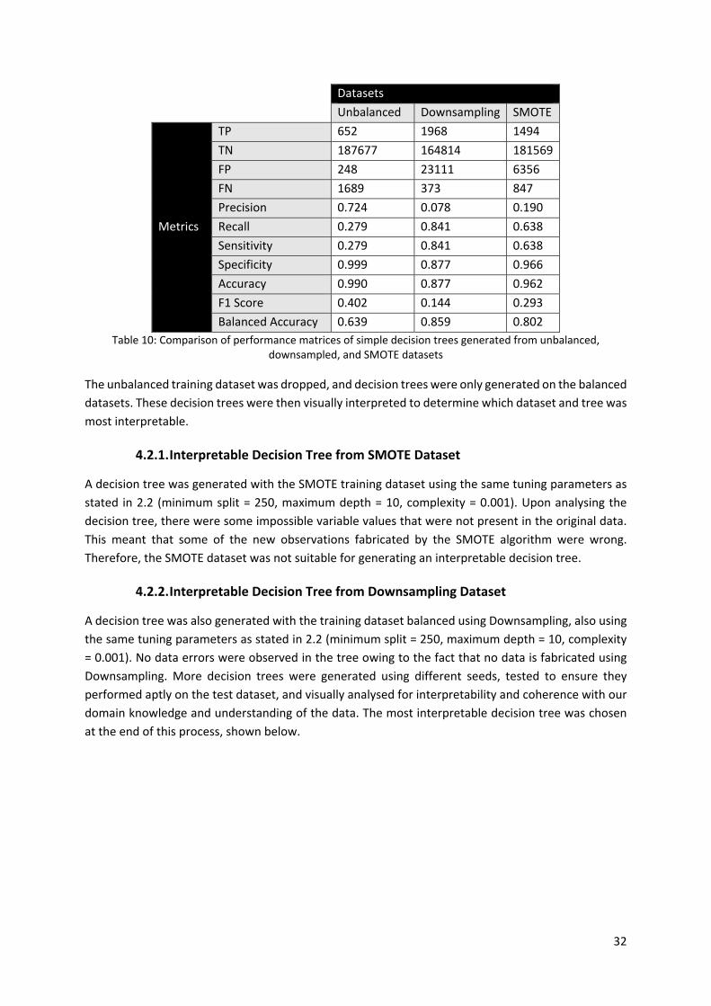
32

Datasets

Unbalanced Downsampling SMOTE

Metrics

TP 652 1968 1494

TN 187677 164814 181569

FP 248 23111 6356

FN 1689 373 847

Precision 0.724 0.078 0.190

Recall 0.279 0.841 0.638

Sensitivity 0.279 0.841 0.638

Specificity 0.999 0.877 0.966

Accuracy 0.990 0.877 0.962

F1 Score 0.402 0.144 0.293

Balanced Accuracy 0.639 0.859 0.802

Table 10: Comparison of performance matrices of simple decision trees generated from unbalanced, downsampled, and SMOTE datasets

The unbalanced training dataset was dropped, and decision trees were only generated on the balanced

datasets. These decision trees were then visually interpreted to determine which dataset and tree was

most interpretable.

4.2.1. Interpretable Decision Tree from SMOTE Dataset

A decision tree was generated with the SMOTE training dataset using the same tuning parameters as

stated in 2.2 (minimum split = 250, maximum depth = 10, complexity = 0.001). Upon analysing the

decision tree, there were some impossible variable values that were not present in the original data.

This meant that some of the new observations fabricated by the SMOTE algorithm were wrong.

Therefore, the SMOTE dataset was not suitable for generating an interpretable decision tree.

4.2.2. Interpretable Decision Tree from Downsampling Dataset

A decision tree was also generated with the training dataset balanced using Downsampling, also using

the same tuning parameters as stated in 2.2 (minimum split = 250, maximum depth = 10, complexity

= 0.001). No data errors were observed in the tree owing to the fact that no data is fabricated using

Downsampling. More decision trees were generated using different seeds, tested to ensure they

performed aptly on the test dataset, and visually analysed for interpretability and coherence with our

domain knowledge and understanding of the data. The most interpretable decision tree was chosen

at the end of this process, shown below.

33

Figure 39: Interpretable decision tree explaining which variables lead to a service request about the lack of TV access

Interpretation of the Decision Tree

Each node of the decision tree has three values: The one at the top indicates the predicted class –

Service Request (SR) or No Service Request (NoSR) at that node of the tree. The second value at the

bottom left indicates the likelihood or probability of the classification. The third value at the bottom

right indicates the percentage of the total training dataset explained by that particular branch of the

decision tree.

The main conclusions from the decision tree were:

1. Pattern 1 – If there were reboots registered then it was 97% likely to be a service request. This

explained 17% of the dataset. This pattern suggests that in most cases the equipment is

rebooted at least once before a service request is made. The reboot could be initiated by the

user or self‐initiated by the equipment to rectify a malfunction ‐ the data doesn’t distinguish

between manual and automatic reboots.

2. Pattern 2 – If there were no reboots, uploads were either minimal or not registered at the hour

of service request, but were registered in the previous hour, then it is 96% likely to be a service

request. This explained an additional 7% of the dataset. This pattern identifies the use case

where there was an interruption in the user’s viewing experience – the user had no access to

the TV service at the time of the service request, but had been watching TV before the

disruption.

3. Pattern 8 – If there were no reboots registered, there were uploads registered and greater

than zero, and there was no usage registered, then it was not likely to be a service request

34

with 80% probability. This prediction explained an additional 44% of the dataset. This pattern

suggests what could be indicative of normal service. If there are no reboots and there are

uploads registered, then the user is likely to have access to their TV service.

4.3. “BLACKBOX” PREDICTIVE MODELS

A “Blackbox” predictive model is a term that refers to predictive models that are not easily

interpretable but whose focus is on predictive accuracy. After basic data understanding was achieved

through the interpretable decision tree described in the previous section, the next step was to produce

more complex predictive models for better predictive accuracy. Four modelling methods were

explored for this purpose: a complex (pruned) decision tree, Bayesian GLM, GBM, and Radom Forest.

Each of these models was tested on both the SMOTE dataset and the Downsampling dataset using the

caret R package and 5‐fold cross‐validation.

The following subsections describe the tuning parameters and results of each of the models.

4.3.1. Tuning Parameters for the Predictive Models

4.3.1.1. Complex Decision Tree

Besides the simple decision tree tuned for interpretability, another more complex decision tree was

generated that was optimized and pruned for predictive accuracy. The complexity parameter was set

to 0.000000001 (very complex) and the minimum split was set to 100, and a decision tree was

generated with these parameters. An optimal complexity parameter was determined by selecting the

complexity parameter than had the lowest ‘xerror’ (cross‐validation prediction error), and the tree is

pruned with this optimal complexity. In R code, this was achieved by the following statements:

optimal.cp <‐ decision.tree$cptable[which.min(decision.tree$cptable[,"xerror"]),"CP"]

pruned.tree <‐ prune(decision.tree, cp=optimal.cp)

The pruned decision tree was then tested on each of the balanced datasets, and its performance is

shown in Section 4.3.2.

4.3.1.2. Bayesian Generalized Linear Model (GLM)

No tuning parameters were need for the Bayesian generalized linear model on the caret R package.

4.3.1.3. Gradient Boosted Machine (GBM)

The GBM method was tested with the following tuning parameters, and its performance is shown in

Section 4.3.2.

Parameter Values Tested

Interaction depth 8, 9, 10, 12

Number of trees 700, 1000, 1200, 1500

Shrinkage 0.01, 0.03, 0.05, 0.07, 0.09, 0.11

Minimum observations in node 10, 20, 30

Sampling down, smote

Table 11: Tuning parameters tested for the GBM model

35

Based on the caret training function with the above parameters, using 5‐fold cross‐validation and ROC

as the metric, it was found that the following were the optimal parameters:

Number of trees = 1200

Interaction depth = 12

Shrinkage = 0.07

Minimum observations in node = 30

4.3.1.4. Random Forest

The random forest method was tested with the following tuning parameters, and its performance is

shown in Section 4.3.2.

Parameter Values Tested

Number of variables randomly sampled at each split (mtry) 6, 7, 8, 9, 10

Number of trees 1000, 1200, 1500

Sampling Down, smote

Table 12: Tuning parameters tested for the GBM model

Based on the caret training function with the above parameters, using 5‐fold cross‐validation and ROC

as a metric, it was found that the following were the optimal parameters:

Number of trees = 1000

Mtry = 10

4.3.2. Comparison of Predictive Model Results

All four models were fed the unbalanced dataset (described in section 4.1), using the caret R package

and cross‐validation. Class balancing was done through caret before cross‐validation. The confusion

matrices of the results of each predictive model were then used to calculate the precision, recall,

sensitivity, specificity, F1 score, accuracy and balanced accuracy of each predictive model. These

results have been summarized in the table below.

Precision Recall Sensitivity Specificity Accuracy

F1

Score

Balanced

Accuracy

Simple

DT

Downsampling 0.078 0.841 0.841 0.877 0.877 0.144 0.859

SMOTE 0.19 0.638 0.638 0.966 0.962 0.293 0.802

Complex

DT

Downsampling 0.095 0.839 0.839 0.901 0.9 0.171 0.87

SMOTE 0.182 0.711 0.711 0.96 0.957 0.29 0.836

GBM Downsampling 0.097 0.864 0.864 0.906 0.905 0.174 0.885

SMOTE 0.135 0.813 0.813 0.939 0.937 0.231 0.876

Random

Forest

Downsampling 0.099 0.863 0.863 0.902 0.901 0.177 0.882

SMOTE 0.12 0.831 0.831 0.924 0.923 0.21 0.878

Bayes

GLM

Downsampling 0.09 0.796 0.796 0.9 0.899 0.162 0.848

SMOTE 0.095 0.782 0.782 0.908 0.906 0.17 0.845

Table 13: Comparison of the performance metrics of each predictive models

36

The decision trees generated using the SMOTE dataset had extremely poor sensitivity, which was

reflected in poor balanced accuracy. The decision trees generated using the down sample dataset were

relatively more effective, but still obtained poor specificity, F1 scores, and balanced accuracy

compared to the other predictive models.

The Bayesian GLM model obtained poor sensitivity scores for both the down sampled and SMOTE

datasets, and was therefore also dismissed as ineffective for the purpose of the project.

The ensemble algorithms (Random Forest and GBM) were the most consistent among the ones

explored, as expected. They had the best balanced accuracy and relatively high F1 score. Among them,

the GBM model that ran on the SMOTE dataset was chosen as the winning model because it performed

well by all performance measures, which was summarised by a high balanced accuracy and F1 score.

4.4. PREDICTIVE MODEL RESULTS AND DISCUSSION

As concluded in the previous section, the winning predictive algorithm for the business needs was the

GBM model applied to data balanced using the SMOTE algorithm. On average, it was able to identify

81.3% (sensitivity) of the users who did not have access to their TV service, and 93.9% of the users who

did have access. The confusion matrix of its performance is shown below.




Table 14: Confusion matrix of GBM results on SMOTE dataset

From the confusion matrix, it can be seen that 38,523 customers (6%) were falsely identified as having

no access to the TV service (false‐positives). Some of these customers may have had an issue accessing

the TV service, but either may not have noticed or may not complained. Others could have been falsely

identified has having no access, either due to an error in the GBM predictive algorithm or the

monitoring data it was fed. There was no way of determining which were the customers that had an

issue but didn’t complain, and which were wrongly identified, based on the monitoring data that was

available.

There are also clients who complained that may have had issues with the settings on the TV itself, and

these client‐side issues cannot be tracked by the monitoring systems. Also, the systems do periodic

monitoring, and so brief service outages may not be picked up by them. These limitations in the

working mechanism of the monitoring system could also explain some of the misclassification of the

predictive model.

37

The top 10 most important variables according to the GBM model are listed in the table below.

Importance Variable Description

1 Number of reboots at the time of complaint

2 Last time watched in minutes (Delta between complaint time and last watched)

3 Volume of data uploaded at the hour of service request

4 Volume of data downloaded at the hour of service request

5 Amount of TV watched at the hour of complaint

6 Ratio of codeword errors received by CMTS related to CM ‐ Ratio of upstream errors in the cell at the time of complaint

7 Volume of data uploaded one hour before the service request

8 Volume of data downloaded one hour before the service request

9 Volume of data downloaded two hours before the service request

10 How long the user was a client

Table 15: Top 10 variables used by the GBM model

If compared to the interpretable decision tree (Figure 40), both models reveal that the number of

reboots registered is the best indicator of no access. They also concur that the volume of uploads and

downloads registered, and usage activity are important indicators of no access.

38

5. CONCLUSIONS

The objectives of this project were to understand the company’s TV customers’ viewing behaviour,

and to explore the possibility of identifying customers who have no access to the TV service, based on

patterns in the data logged by in‐house monitoring systems. Both these objectives were part of an

ongoing effort by the company to improve the quality of its TV service, and to curtail customer

dissatisfaction and churn. The success of the project could not be quantified because of the

investigatory nature of both the objectives. Instead, it was assessed based on the value and insight it

drew from the large volumes of monitoring data (much of which was previously unexplored), that

could inform decision‐makers of future work in the area. By this measure, the project was a success!

Machine learning algorithms revealed patterns in the monitoring system data that lead to valuable

insights.

The K‐means++ clustering algorithm was able to cluster the customer base into six segments, which

were then analysed to formulate user profiles based on viewing patterns. These user profiles were:

Average TV users, Light TV users, Heavy TV users, HD TV users, Light TV App users, and Heavy TV App

users. Though these user profiles were created from data from February 2018, they also appeared in

the data from March and April 2018, and is expected to be consistent across other months as well.

These user profiles helped the company better understand their customers’ viewing behaviour and

potentially gauge how much of an impact the lack of access to the TV service could have on them at a

given time.

A predictive model was developed to identify users who have no access to the TV service. It used

SMOTE to balance the unbalanced input data, and used the GBM algorithm for supervised learning.

The predictive model was able to identify approximately 80% of the users who had no access to the

service, with a false‐positive rate of 6%. Some of the customers among the false‐positives may have

had an issue with lack of access, but did not complain about it. However, real‐world testing would be

required to identify these customers among the false‐positives. Nonetheless, it was believed that the

majority of the false‐positives were indeed wrongly classified. Limitations in the data and human error

in data collection and labelling are likely contributors to the error. Further tweaking of the predictive

modelling process may also improve the end result. The limitations and recommendations for future

work on the project have been described in greater detail in the next segment of the report.

39

6. LIMITATIONS AND RECOMMENDATIONS FOR FUTURE WORKS

Though the project was an overall success, there were limitations in the data, and clustering and

predictive modelling process to be aware of and possibly improve upon.

Here are some data limitations that were identified:

1. Each monitoring system collects data at an arbitrary point within an hour. It is possible that

one monitoring system gathers readings at the beginning of the hour while the other at the

end. Therefore, the timestamps of data logged by the monitoring systems are not perfectly

synced.

2. There is a human‐error factor with respect to determining what complains are labelled as a

“no access” issue. The user may have complained about lack of access, but it may have been

another type of issue. This would cause noise in the complaints dataset.

3. The “number of reboots” variable is an important discriminating variable according to the

predictive algorithms, but it doesn’t distinguish between automatic and manual reboots.

There were other limitations in the project due to resource constraints. These limitations have been

listed below along with recommendations:

1. In the real world, there usually is a time gap between the time of the user lost access to the

TV service, when it was noticed, and when it was called in. This time gap wasn’t well accounted

for in the current process – only 3 hours of data was collected prior to the service request.

Recommendation – Collect monitoring data from more data points prior to complaint. If

more data is available, time‐series analysis could be explored to determine if disruption in

the service happens gradually or abruptly.

2. Only data from February 2018 was analysed, and tested on data from March and April 2018.

An assumption was made that the clusters would also be consistent across other months.

Recommendation – Test and re‐cluster the data for all 12 months (or more), to account

for seasonality and trends in viewing behaviour. Also test the assumption that the clusters

remain unchanged throughout the year – it is possible that different months may have

different clusters (including number of clusters) due to seasonality, e.g. there may be a

“sports viewers” cluster during the football season.

3. Only a few clustering algorithms and methods for finding optimal number of clusters were

explored.

Recommendation – Try more algorithms to see if there is one better than K‐means++ for

the data and the business needs.

4. During the data gathering step, it was assumed that people who didn’t complain had no issue

with the service, and that the couple of timestamps chosen for collecting data (February 2, 17h

to 19h and February 14, 12h – 15h) were representative of the population who had access to

the service.

Recommendation – Collect more data points from different times of the day and different

days of the week. If possible, collect population data at the same time as the complaints

occurred.

5. Only 4 predictive algorithms were explored due to constraints in time and processing power.

Recommendation – Explore more predictive algorithms and ensembles to determine if

there is better alternative to GBM in terms of time efficiency or predictive accuracy.

40

7. BIBLIOGRAPHY

Castle, N. Supervised vs. Unsupervised Machine Learning. Retrieved from

https://www.datascience.com/blog/supervised‐and‐unsupervised‐machine‐learning‐algorithms

Abdi, H., & Williams, L. (2010). Principal component analysis. Wiley Interdisciplinary Reviews:

Computational Statistics, 2(4), 433‐459. doi: 10.1002/wics.101

Arthur, D., & Vassilvitskii, S. (2006). k‐means++: The Advantages of Careful Seeding. Retrieved from

http://ilpubs.stanford.edu:8090/778/1/2006‐13.pdf

Cliff, N. (1988). The eigenvalues‐greater‐than‐one rule and the reliability of components.

Psychological Bulletin, 103(2), 276‐279. doi: 10.1037//0033‐2909.103.2.276

Kassambara, A. (2017). Determining The Optimal Number Of Clusters: 3 Must Know Methods ‐

Articles ‐ STHDA. Retrieved from http://www.sthda.com/english/articles/29‐cluster‐validation‐

essentials/96‐determining‐the‐optimal‐number‐of‐clusters‐3‐must‐know‐methods/#computing‐the‐

number‐of‐clusters‐using‐r

Kaufman, L., & Rousseeuw, P. (2018). R: Clustering Large Applications. Retrieved from

https://stat.ethz.ch/R‐manual/R‐devel/library/cluster/html/clara.html

Mann, A., & Kaur, N. (2013). Review Paper on Clustering Techniques. Global Journal Of Computer

Science And Technology Software & Data Engineering, 13(5). Retrieved from

https://pdfs.semanticscholar.org/12f4/a1852e95939080b695edbb7d23183918689e.pdf

Rousseeuw, P. (1987). Silhouettes: A graphical aid to the interpretation and validation of cluster

analysis. Journal Of Computational And Applied Mathematics, 20, 53‐65. doi: 10.1016/0377‐

0427(87)90125‐7

Sileshi, M., & Gamback, B. (2018). Evaluating Clustering Algorithms: Cluster Quality and Feature

Selection in Content‐Based Image Clustering. In 2009 WRI World Congress on Computer Science and

Information Engineering. Los Angeles, CA, USA: IEEE. Retrieved from

https://ieeexplore.ieee.org/document/5170736/

Tibshirani, R., Walther, G., & Hastie, T. (2001). Estimating the number of clusters in a data set via the

gap statistic. Journal Of The Royal Statistical Society: Series B (Statistical Methodology), 63(2), 411‐

423. doi: 10.1111/1467‐9868.00293

Trevino, A. (2018). Introduction to K‐means Clustering. Retrieved from

https://www.datascience.com/blog/k‐means‐clustering

Van der Laan, M., Pollard, K., & Bryan, J. (2003). A new partitioning around medoids algorithm.

Journal Of Statistical Computation And Simulation, 73(8), 575‐584. doi:

10.1080/0094965031000136012

Kadir, S., Goodman, D., & Harris, K. (2014). High‐Dimensional Cluster Analysis with the Masked EM

Algorithm. Neural Computation, 26(11), 2379‐2394. doi: 10.1162/neco_a_00661

41

UC Business Analytics R Programming Guide. K‐means Cluster Analysis. Retrieved from https://uc‐

r.github.io/kmeans_clustering

Gap Statistic. (2018). Retrieved from https://datasciencelab.wordpress.com/tag/gap‐statistic/

Upsana. (2017). How to handle Imbalanced Classification Problems in machine learning?. Retrieved

from https://www.analyticsvidhya.com/blog/2017/03/imbalanced‐classification‐problem/

Brownlee, J. (2017). Difference Between Classification and Regression in Machine Learning. [online]

Machine Learning Mastery. Available at: https://machinelearningmastery.com/classification‐versus‐

regression‐in‐machine‐learning/.

Garg, R. (2018). A Primer to Ensemble Learning – Bagging and Boosting. [online] Analytics India

Magazine. Available at: https://analyticsindiamag.com/primer‐ensemble‐learning‐bagging‐boosting/.

Gerwinn, S. (2010). Bayesian inference for generalized linear models for spiking neurons. Frontiers in

Computational Neuroscience, 4.

Grover, P. (2017). Gradient Boosting from scratch – ML Review – Medium. [online] Medium. Available

at: https://medium.com/mlreview/gradient‐boosting‐from‐scratch‐1e317ae4587d.

Investopedia (2018). Predictive Modeling. [online] Investopedia. Available at:

https://www.investopedia.com/terms/p/predictive‐modeling.asp.

Kotsiantis, S. (2011). Decision trees: a recent overview. Artificial Intelligence Review, 39(4), pp.261‐

283.

Kulkarni, M. (2017). Decision Trees for Classification: A Machine Learning Algorithm | Xoriant Blog.

[online] Xoriant Blog. Available at: https://www.xoriant.com/blog/product‐engineering/decision‐

trees‐machine‐learning‐algorithm.html.

Nagpal, A. (2017). Decision Tree Ensembles‐ Bagging and Boosting – Towards Data Science. [online]

Towards Data Science. Available at: https://towardsdatascience.com/decision‐tree‐ensembles‐

bagging‐and‐boosting‐266a8ba60fd9.

Navlani, A. (2018). Understanding Random Forests Classifiers in Python. [image] Available at:

https://www.datacamp.com/community/tutorials/random‐forests‐classifier‐python.

Quantdare (2016). What is the difference between Bagging and Boosting?. [image] Available at:

https://quantdare.com/what‐is‐the‐difference‐between‐bagging‐and‐boosting/.

Starkweather, J. (2011). Bayesian Generalized Linear Models in R. [online] Available at:

https://it.unt.edu/sites/default/files/bayesglm_jds_jan2011.pdf.

StatSoft (2004). Electronic statistics textbook. Tulsa: StatSoft.

Becker, D. (n.d.). Cross‐Validation | Kaggle. [online] Kaggle.com. Available at:

https://www.kaggle.com/dansbecker/cross‐validation.

Data School (2014). Simple guide to confusion matrix terminology. [online] Data School. Available at:

https://www.dataschool.io/simple‐guide‐to‐confusion‐matrix‐terminology/.

42

Donges, N. (2018). Gradient Descent in a Nutshell – Towards Data Science. [online] Towards Data

Science. Available at: https://towardsdatascience.com/gradient‐descent‐in‐a‐nutshell‐eaf8c18212f0.

Grace‐Martin, K. (n.d.). What Is an ROC Curve?. [online] Theanalysisfactor.com. Available at:

https://www.theanalysisfactor.com/what‐is‐an‐roc‐curve/.

Natekin, A. and Knoll, A. (2013). Gradient boosting machines, a tutorial. Frontiers in Neurorobotics, 7.

Srivastava, T. (2016). 7 Important Model Evaluation Error Metrics Everyone should know. [online]

Analytics Vidhya. Available at: https://www.analyticsvidhya.com/blog/2016/02/7‐important‐model‐

evaluation‐error‐metrics/.

UC Business Analytics R Programming Guide (n.d.). Gradient Boosting Machines ∙ UC Business

Analytics R Programming Guide. [online] Uc‐r.github.io. Available at: http://uc‐

r.github.io/gbm_regression.

WebFOCUS (2015). Explanation of the Decision Tree Mode. [online] WebFOCUS Release 8.0 Versions

10 and 09 Technical Library. Available at:

https://infocenter.informationbuilders.com/wf80/index.jsp?topic=%2Fpubdocs%2FRStat16%2Fsourc

e%2Ftopic47.htm.

Breiman, L. and Cutler, A. (2018). Breiman and Cutler's Random Forests for Classification and

Regression. [online] Cran.r‐project.org. Available at: https://cran.r‐

project.org/web/packages/randomForest/randomForest.pdf.

Bhalla, D. (n.d.). GBM (Boosted Models) Tuning Parameters. [online] ListenData. Available at:

https://www.listendata.com/2015/07/gbm‐boosted‐models‐tuning‐parameters.html.

Steinbach, M., Ertöz, L. and Kumar, V. (2002). The Challenges of Clustering High Dimensional Data.

an application of user segmentation and modelling at a

Documents