an efﬁcient algorithm for computing the baker–campbell ... · 1departament de matemàtiques,...

An efficient algorithm for computingthe Baker–Campbell–Hausdorff seriesand some of its applications

Fernando Casas1,a� and Ander Murua2,b�

1Departament de Matemàtiques, Universitat Jaume I, E-12071 Castellón, Spain2Konputazio Zientziak eta A.A. saila, Informatika Fakultatea, EHU/UPV,E-20018 Donostia/San Sebastián, Spain

�Received 3 November 2008; accepted 5 January 2009; published online 30 March 2009�

We provide a new algorithm for generating the Baker–Campbell–Hausdorff �BCH�series Z=log�eXeY� in an arbitrary generalized Hall basis of the free Lie algebraL�X ,Y� generated by X and Y. It is based on the close relationship of L�X ,Y� witha Lie algebraic structure of labeled rooted trees. With this algorithm, the computa-tion of the BCH series up to degree of 20 �111 013 independent elements inL�X ,Y�� takes less than 15 min on a personal computer and requires 1.5 Gbytes ofmemory. We also address the issue of the convergence of the series, providing anoptimal convergence domain when X and Y are real or complex matrices. © 2009American Institute of Physics. �DOI: 10.1063/1.3078418�

I. INTRODUCTION

The Baker–Campbell–Hausdorff �BCH� formula deals with the expansion of Z in eXeY =eZ interms of nested commutators of X and Y when they are assumed to be noncommuting operators.If we introduce the formal series for the exponential function

eXeY = �p,q=0

�1

p!q!XpYq �1.1�

and substitute this series in the formal series defining the logarithm function

log Z = �k=1

��− 1�k−1

k�Z − 1�k,

one obtains

log�eXeY� = �k=1

��− 1�k−1

k � Xp1Yq1¯ XpkYqk

p1!q1! ¯ pk!qk!,

where the inner summation extends over all non-negative integers p1, q1 , . . ., pk, qk for which pi

+qi�0 �i=1,2 , . . . ,k�. Gathering together the terms for which p1+q1+ p2+q2+ ¯ + pk+qk=m, wecan write

a�Author to whom correspondence should be addressed. Electronic addresses: [email protected]�Electronic mail: [email protected].

JOURNAL OF MATHEMATICAL PHYSICS 50, 033513 �2009�

50, 033513-10022-2488/2009/50�3�/033513/23/$25.00 © 2009 American Institute of Physics

Author complimentary copy. Redistribution subject to AIP license or copyright, see http://jmp.aip.org/jmp/copyright.jsp

http://dx.doi.org/10.1063/1.3078418

http://dx.doi.org/10.1063/1.3078418

http://dx.doi.org/10.1063/1.3078418

http://dx.doi.org/10.1063/1.3078418

Z = log�eXeY� = �m=1

�

Pm�X,Y� , �1.2�

where Pm�X ,Y� is a homogeneous polynomial of degree m in the noncommuting variables X andY. Campbell,8 Baker,2 and Hausdorff17 addressed the question whether Z can be represented as aseries of nested commutators of X and Y, without producing a general formula. We recall here thatthe commutator �X ,Y� is defined as XY −YX. It was Dynkin12 who finally derived an explicitformula for Z as

Z = �k=1

�

�pi,qi

�− 1�k−1

k

�Xp1Yq1¯ XpkYqk�

��i=1k �pi + qi��p1!q1! ¯ pk!qk!

. �1.3�

Here the inner summation is taken over all non-negative integers p1 ,q1 , . . . , pk, qk such that p1

+q1�0, . . . , pk+qk�0 and �Xp1Yq1¯XpkYqk� denotes the right nested commutator based on the

word Xp1Yq1¯XpkYqk. Expression �1.3� is known, for obvious reasons, as the BCH series in the

Dynkin form. By rearranging terms, it is clear that Z can be written as

Z = log�eXeY� = X + Y + �m=2

�

Zm, �1.4�

with Zm�X ,Y� a homogeneous Lie polynomial in X and Y of degree m, i.e., it is a Q-linearcombination of commutators of the form �V1 , �V2 , . . . , �Vm−1 ,Vm�¯ �� with Vi� �X ,Y� for 1� i�m. The first terms read explicitly

Z2 = 12 �X,Y� ,

Z3 = 112�X,�X,Y�� − 1

12�Y,�X,Y�� ,

Z4 = 124�X,�Y,�Y,X�� .

The expression eXeY =eZ is then called the BCH formula, although other different labels �e.g.,Campbell–Baker–Hausdorff, Baker–Hausdorff, Campbell–Hausdorff� are commonly attached to itin the literature. The formula �1.3� is certainly awkward to use due to the complexity of the sumsinvolved. Notice, in particular, that different choices of pi, qi, k in �1.3� may lead to terms in thesame commutator. Thus, for instance, �X3Y1�= �X1Y0X2Y1�= �X , �X , �X ,Y��. An additional diffi-culty arises from the fact that not all the commutators are independent due to the Jacobi identity,47

�X1,�X2,X3�� + �X2,�X3,X1�� + �X3,�X1,X2�� = 0.

The BCH formula plays a fundamental role in many fields of mathematics �theory of lineardifferential equations,26 Lie groups,14 numerical analysis16�, theoretical physics �perturbationtheory,10 quantum mechanics,49 statistical mechanics,24,50 quantum computing40�, and controltheory �analysis and design of nonlinear control laws, nonlinear filters, stabilization of rigidbodies46�. In particular, in the theory of Lie groups, with this formula one can explicitly write theoperation of multiplication in a Lie group in canonical coordinates in terms of the Lie bracketoperation in its tangent algebra and also prove the existence of a local Lie group with a given Liealgebra.14

Also in the numerical treatment of differential equations on manifolds,19,16 the BCH formulais quite useful. If M is a smooth manifold and X�M� denotes the linear space of smooth vectorfields on M, then a Lie algebra structure is established in X�M� by using the Lie bracket �X ,Y�of fields X and Y �X�M�.47 The flow of a vector field X�X�M� is a mapping exp�X� definedthrough the solution of the differential equation

033513-2 F. Casas and A. Murua J. Math. Phys. 50, 033513 �2009�


du

dt= X�u�, u�0� = q � M �1.5�

as exp�tX��q�=u�t�. Many numerical methods used to approximately solve Eq. �1.5� are based oncompositions of maps that are flows of vector fields.16 To be more specific, suppose the vectorfield X can be split as X=A+B and that the flows corresponding to A�u� and B�u� can be explicitlyobtained. Then one may consider an approximation of the form �h

�exp�ha1A�exp�hb1B�¯exp�hakA�exp�hbkB� for the exact flow exp�h�A+B�� of �1.5� after atime step h. The idea now is to obtain the conditions to be satisfied by the coefficients ai, bi so that�h�q�=u�h�+O�hp+1� as h→0, and this can be done by applying the BCH formula in sequence tothe expression of � up to the degree required by the order of approximation p.27 This task can becarried out quite easily provided one has explicit expressions of Zm implemented in a symbolicalgebra package.23,46

In addition to the Dynkin form �1.3�, there are other standard procedures to construct explic-itly the BCH series. Recall that the free Lie algebra L�X ,Y� generated by the symbols X and Y canbe considered as a subspace �the subspace of Lie polynomials� of the vector space spanned by thewords w in the symbols X and Y, i.e., w=a1a2¯am, each ai being X or Y. Thus, the BCH seriesadmits the explicit associative presentation

Z = X + Y + �m=2

�

�w,w=m

gww , �1.6�

in which gw is a rational coefficient and the inner sum is taken over all words w with length w=m. Here the length of w is the number of letters it contains. The coefficients can be computedwith a procedure based on a family of recursively computable polynomials.13

Although the terms in Eq. �1.6� are expressed as linear combinations of individual words�which are not Lie polynomials�, by virtue of the Dynkin–Specht–Wever theorem,21 Z can bewritten as

Z = X + Y + �m=2

�1

m �w,w=m

gw�w� , �1.7�

that is, the individual terms are the same as in the associative series �1.6� except that the wordw=a1a2¯am is replaced with the right nested commutator �w�= �a1 , �a2 , . . . , �am−1 ,am�¯ �� andthe coefficient gw is divided by the word length m.42 This gives explicit expressions of the termsZm in the BCH series �1.4� as a linear combination of nested commutators of homogeneous degree,that is, as a linear combination of elements of the homogeneous subspace L�X ,Y�m of degre m ofthe free Lie algebra L�X ,Y�. However, it should be stressed that the set of nested commutators �w�for words w of length m is not a basis of the homogeneous subspace L�X ,Y�m.

By introducing a parameter � and differentiating with respect to � the power series�m�1�mZm=log�exp��X�exp��Y��, the following recursion formula is derived in Ref. 47:

Z1 = X + Y ,

�1.8�

mZm =1

2�X − Y,Zm−1� + �

p=1

��m−1�/2�B2p

�2p�!�adZ

2p�X + Y��m, m � 1.

Here Z=�m�1Zm, adZk�X+Y�= �Z , adZ

k−1�X+Y��, the Bj stand for the Bernoulli numbers,1 and�adZ

2p�X+Y��m denotes the projection of adZ2p�X+Y� onto the homogeneous subspace L�X ,Y�m,

which can be written in terms of Z1 ,Z2 ,Z3 , . . . as

033513-3 Efficient computation of the BCH series J. Math. Phys. 50, 033513 �2009�


�adZ2p�X + Y��m = �

k1+¯+k2p=m−1

k1�1,. . .,k2p�1

�Zk1,�¯�Zk2p

,X + Y� ¯ �� .

Explicit formulas �1.3� and �1.7�, as well as recursion �1.8� can be used in principle toconstruct the BCH series up to arbitrary degree in terms of commutators. As a matter of fact,several systematic computations of the series have been carried out along the years, starting withthe work of Richtmyer and Greenspan in 1965,37 where results up to degree of 8 are reported.Later on, Newman and Thompson obtained the coefficients gw in �1.7� up to words of length of20,32 Bose6 constructed an algorithm to compute directly the coefficient of a given commutator inthe Dynkin presentation �1.3� and Oteo33 and Kolsrud22 presented a simplified expression of �1.3�in terms of right nested commutators up to degrees of 8 and 9, respectively. More recently,Reinsch35 proposed a matrix operation procedure for calculating the polynomials Pm�X ,Y� in �1.2�which can be easily implemented in any symbolic algebra package. Again, the Dynkin–Specht–Wever has to be used to write the resulting expressions in terms of commutators.

As mentioned before, all of these procedures exhibit a key limitation, however: the iteratedcommutators are not all linearly independent due to the Jacobi identity �and other identitiesinvolving nested commutators of higher degree which are originated by it33�. In other words, theydo not provide expressions directly in terms of a basis of the free Lie algebra L�X ,Y�. This isrequired, for instance, in applications of the BCH formula in the numerical integration of ordinarydifferential equations or when one wants to study specific features of the series, such as thedistribution of the coefficients and other combinatorial properties.32

Of course, it is always possible to express the resulting formulas in terms of a basis of L�X ,Y�but this rewriting process is very time consuming and requires a good deal of memory resources.In practice, going beyond degree m=11 constitutes a difficult task indeed,28,23,46 since the numberof terms involved in the series grows, in general, as the dimension cm of the homogeneoussubspace L�X ,Y�m. As is well known, cm is given by the Witt formula,7 so that cm=O�2m /m�.

Our goal is then to express the BCH series as

Z = log�exp�X�exp�Y�� = �i�1

ziEi, �1.9�

where zi�Q �i�1� and �Ei : i=1,2 ,3 , . . . � is a basis of L�X ,Y� whose elements are of the form

E1 = X, E2 = Y, and Ei = �Ei�,Ei��, i � 3, �1.10�

for appropriate values of the integers i� , i�� i �for i=3,4 , . . .�. Clearly, each Ei in �1.10� is ahomogeneous Lie polynomial of degree i, where

1 = 2 = 1 and i = i� + i� for i � 3. �1.11�

We will focus on a general class of bases of the free Lie algebra L�X ,Y�, referred to in the currentliterature as generalized Hall bases and also as Hall–Viennot bases.36,48 These include the Lyndonbasis25,48 and different variants of the classical Hall basis �see Ref. 36, for references�. Specifically,in this paper we present a new procedure to write the BCH series �1.9� for an arbitrary Hall–Viennot basis. Such an algorithm is based on results obtained in Ref. 30, in particular, thoserelating a certain Lie algebra structure g on rooted trees with the description of a free Lie algebrain terms of a Hall basis. This Lie algebra g on rooted trees was first considered in Ref. 11, whereasa closely related Lie algebra on labeled rooted trees was treated in Ref. 15 �see Ref. 18 for therelation of these two Lie algebras and for further references about related algebraic structures onrooted trees�.

We have implemented the algorithm in MATHEMATICA �it can also be programmed in FORTRAN

or C for more efficiency�. The resulting procedure gives the BCH series up to a prescribed degreedirectly in terms of a Hall–Viennot basis of L�X ,Y�. As an illustration, obtaining the series �in theclassical basis of P. Hall� up to degree m=20 with a personal computer �2.4 GHz Intel Core 2 Duo



processor with 2 Gbytes of random access memory� requires less than 15 min of CPU time and1.5 Gbytes of memory. The resulting expression has 109 697 nonvanishing coefficients out of111 013 elements Ei of degree i�20 in the Hall basis. As far as we know, there are no results upto such a high degree reported in the literature. For comparison with other procedures, the authorsof Ref. 46 reported 25 h of CPU time and 17.5 Mbytes with a Pentium III personal computer toachieve degree of 10. By contrast, our algorithm is able to achieve m=10 in 0.058 s and onlyneeds 5.4 Mbytes of computer memory.

In Table III in the Appendix, we give the values of i� and i� for the elements Ei of degreei�9 in the Hall basis and their coefficients zi in the BCH formula �1.9�. The elements of the basisare ordered in such a way that i� j if i� j, and the horizontal lines in the table separate elementsof different homogeneous degree. Extension of Table III up to terms of degree of 20 is availableat the website www.gicas.uji.es/research/bch.html for both the basis of P. Hall and the Lyndonbasis. As an example, the last element of degree of 20 in the Hall basis is

E111013 = ��Y,X�,Y�,�Y,X��,��Y,X�,X�,�Y,X��,��Y,X�,Y�,�Y,X��,��Y,X�,Y�,Y�,Y�� ,

and the corresponding coefficient in �1.9� reads

z111 013 = −19 234 697

140 792 940 288.

Another central issue addressed in this paper concerns the convergence properties of the BCHseries. Suppose we introduce a submultiplicative norm · such that

�X,Y� � �XY �1.12�

for some ��0. Then it is not difficult to show that the series �1.3� is absolutely convergent as longas X+ Y� �log 2� /�.7,41 As a matter of fact, several improved bounds have been obtained forthe different presentations. Thus, in particular, the Lie presentation �1.7� converges absolutely ifX�1 /� and Y�1 /� in a normed Lie algebra g with a norm satisfying �1.12�,31,45 whereas inRef. 3 it has been shown that the series Z=�m�1Zm is absolutely convergent for all X, Y such that

�X � ��Y

2 1

2 +t

2�1 − cot�1

2t dt �1.13�

and the corresponding expression obtained by interchanging in �1.13� X by Y. Moreover, the seriesdiverges, in general, if X+ Y� when �=2.28 Here we provide a generalization of this featurebased on the well known Magnus expansion for linear differential equations26 and also we give amore precise characterization of the convergence domain of the series when X and Y are �real orcomplex� matrices.

II. AN ALGORITHM FOR COMPUTING THE BCH SERIES BASED ON ROOTED TREES

A. Summary of the procedure

Our starting point is the vector space g of maps :T→R, where T denotes the set of rootedtrees with black and white vertices,

In the combinatorial literature, T is typically referred to as the set of labeled rooted trees with twolabels, “black” and “white.” Hereafter, we refer to the elements of T as bicoloured rooted trees.

The vector space g is endowed with a Lie algebra structure by defining the Lie bracket� ,��g of two arbitrary maps ,��g as follows. For each u�T,



�,��u� = �j=1

u=1

��u�j��u�j�� − �u�j��u�j�� , �2.1�

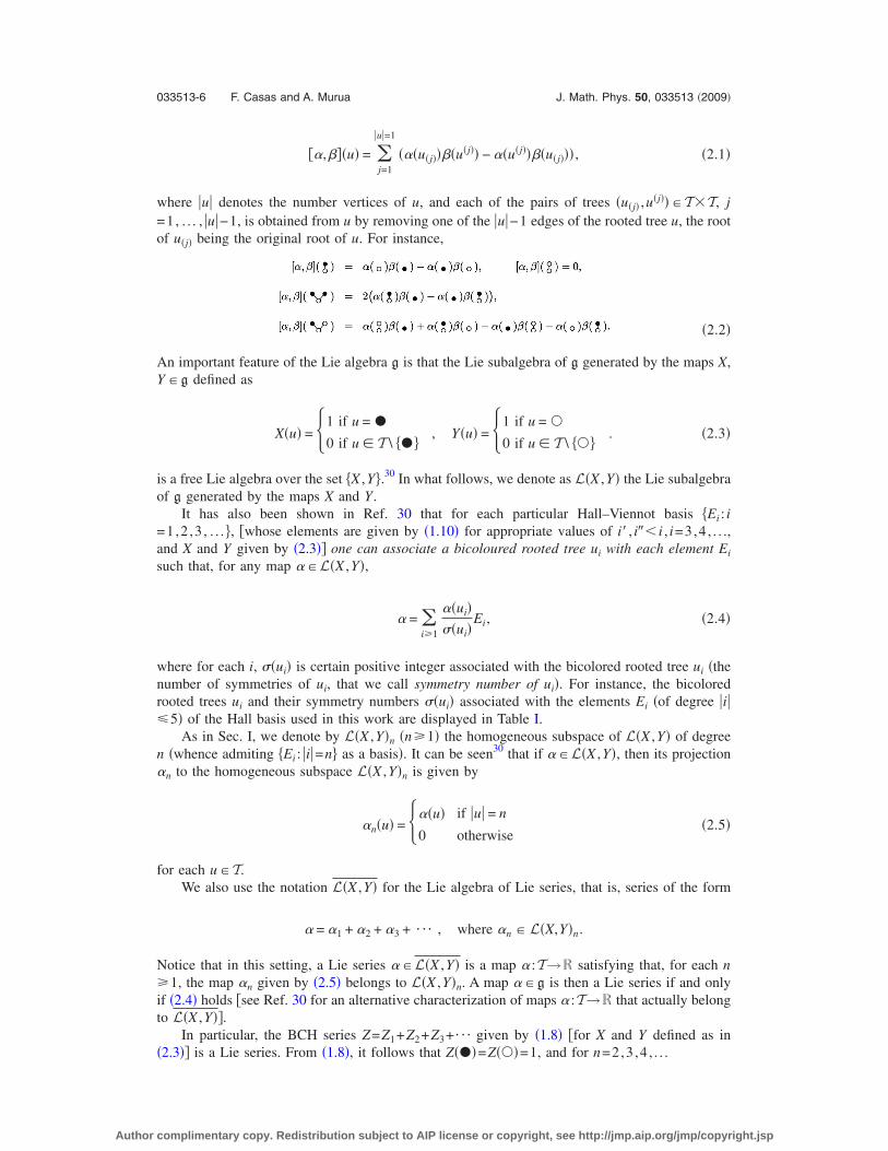
where u denotes the number vertices of u, and each of the pairs of trees �u�j� ,u�j��T�T, j

=1, . . . , u−1, is obtained from u by removing one of the u−1 edges of the rooted tree u, the rootof u�j� being the original root of u. For instance,

�2.2�

An important feature of the Lie algebra g is that the Lie subalgebra of g generated by the maps X,Y �g defined as

X�u� = �1 if u = �0 if u � T \ �� , Y�u� = �1 if u = �

0 if u � T \ �� . �2.3�

is a free Lie algebra over the set �X ,Y�.30 In what follows, we denote as L�X ,Y� the Lie subalgebraof g generated by the maps X and Y.

It has also been shown in Ref. 30 that for each particular Hall–Viennot basis �Ei : i=1,2 ,3 , . . . �, �whose elements are given by �1.10� for appropriate values of i� , i�� i , i=3,4 , . . .,and X and Y given by �2.3�� one can associate a bicoloured rooted tree ui with each element Ei

such that, for any map �L�X ,Y�,

= �i�1

�ui� �ui�

Ei, �2.4�

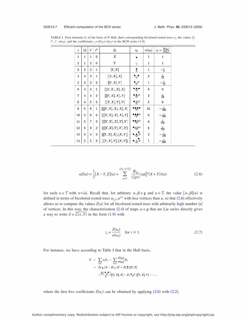
where for each i, �ui� is certain positive integer associated with the bicolored rooted tree ui �thenumber of symmetries of ui, that we call symmetry number of ui�. For instance, the bicoloredrooted trees ui and their symmetry numbers �ui� associated with the elements Ei �of degree i�5� of the Hall basis used in this work are displayed in Table I.

As in Sec. I, we denote by L�X ,Y�n �n�1� the homogeneous subspace of L�X ,Y� of degreen �whence admiting �Ei : i=n� as a basis�. It can be seen30 that if �L�X ,Y�, then its projectionn to the homogeneous subspace L�X ,Y�n is given by

n�u� = ��u� if u = n

0 otherwise� �2.5�

for each u�T.We also use the notation L�X ,Y� for the Lie algebra of Lie series, that is, series of the form

= 1 + 2 + 3 + ¯ , where n � L�X,Y�n.

Notice that in this setting, a Lie series �L�X ,Y� is a map :T→R satisfying that, for each n�1, the map n given by �2.5� belongs to L�X ,Y�n. A map �g is then a Lie series if and onlyif �2.4� holds �see Ref. 30 for an alternative characterization of maps :T→R that actually belongto L�X ,Y��.

In particular, the BCH series Z=Z1+Z2+Z3+¯ given by �1.8� �for X and Y defined as in�2.3�� is a Lie series. From �1.8�, it follows that Z��=Z��=1, and for n=2,3 ,4 , . . .



nZ�u� =1

2�X − Y,Z��u� + �

p=1

��n−1�/2�B2p

�2p�!�adZ

2p�X + Y��u� �2.6�

for each u�T with n= u. Recall that, for arbitrary ,��g and u�T, the value � ,��u� isdefined in terms of bicolored rooted trees u�j� ,u

�j� with less vertices than u, so that �2.6� effectivelyallows us to compute the values Z�u� for all bicolored rooted trees with arbitrarily high number uof vertices. In this way, the characterization �2.4� of maps �g that are Lie series directly givesa way to write Z�L�x ,Y� in the form �1.9� with

zi =Z�ui� �ui�

for i � 1. �2.7�

For instance, we have according to Table I that in the Hall basis,

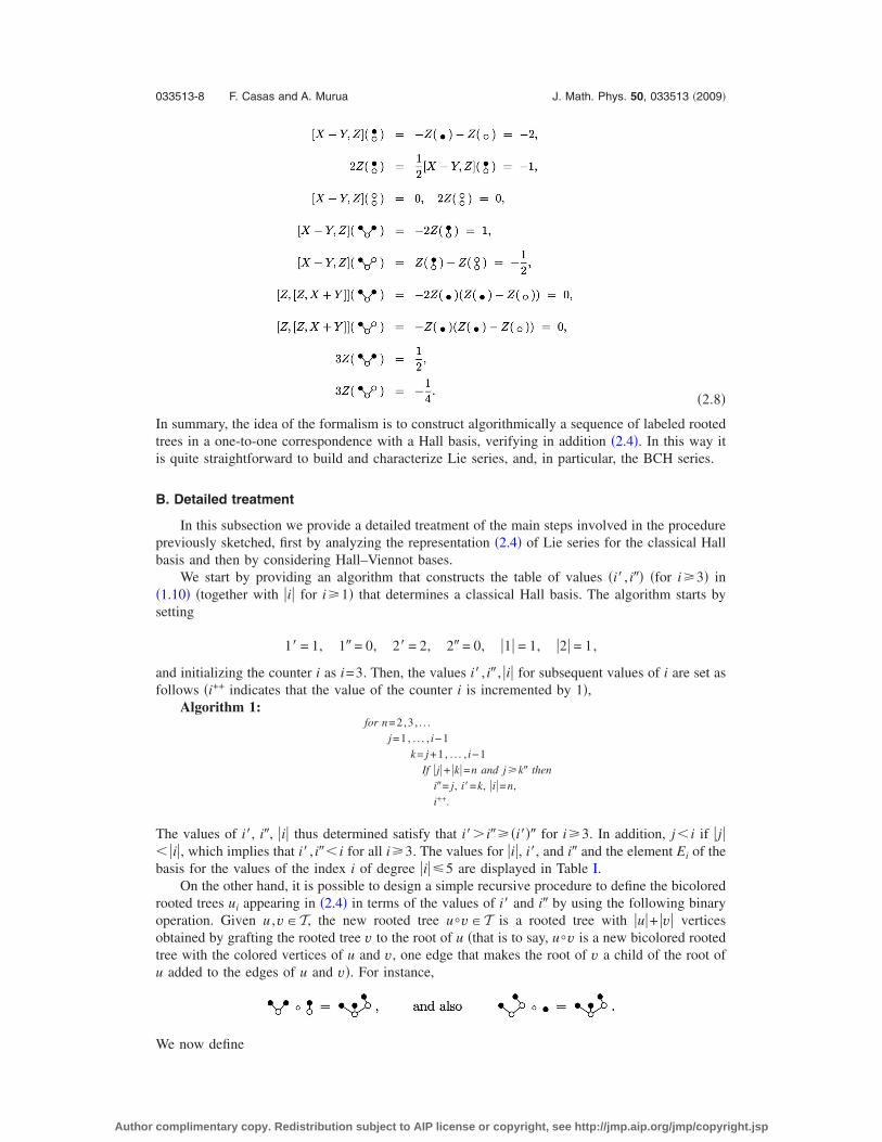
where the first five coefficients Z�ui� can be obtained by applying �2.6� with �2.2�,

TABLE I. First elements Ei of the basis of P. Hall, their corresponding bicolored rooted trees ui, the values i,i�, i�, �ui�, and the coefficients zi=Z�ui� / �ui� in the BCH series �1.9�.



�2.8�

In summary, the idea of the formalism is to construct algorithmically a sequence of labeled rootedtrees in a one-to-one correspondence with a Hall basis, verifying in addition �2.4�. In this way itis quite straightforward to build and characterize Lie series, and, in particular, the BCH series.

B. Detailed treatment

In this subsection we provide a detailed treatment of the main steps involved in the procedurepreviously sketched, first by analyzing the representation �2.4� of Lie series for the classical Hallbasis and then by considering Hall–Viennot bases.

We start by providing an algorithm that constructs the table of values �i� , i�� for i�3� in�1.10� �together with i for i�1� that determines a classical Hall basis. The algorithm starts bysetting

1� = 1, 1� = 0, 2� = 2, 2� = 0, 1 = 1, 2 = 1,

and initializing the counter i as i=3. Then, the values i� , i� , i for subsequent values of i are set asfollows �i++ indicates that the value of the counter i is incremented by 1�,

Algorithm 1:for n=2,3 , . . .

j=1, . . . , i−1k= j+1, . . . , i−1

If j+ k=n and j�k� theni�= j, i�=k, i=n,i++.

The values of i�, i�, i thus determined satisfy that i�� i�� i�� for i�3. In addition, j� i if j� i, which implies that i� , i�� i for all i�3. The values for i, i�, and i� and the element Ei of thebasis for the values of the index i of degree i�5 are displayed in Table I.

On the other hand, it is possible to design a simple recursive procedure to define the bicoloredrooted trees ui appearing in �2.4� in terms of the values of i� and i� by using the following binaryoperation. Given u ,v�T, the new rooted tree u �v�T is a rooted tree with u+ v verticesobtained by grafting the rooted tree v to the root of u �that is to say, u �v is a new bicolored rootedtree with the colored vertices of u and v, one edge that makes the root of v a child of the root ofu added to the edges of u and v�. For instance,

We now define



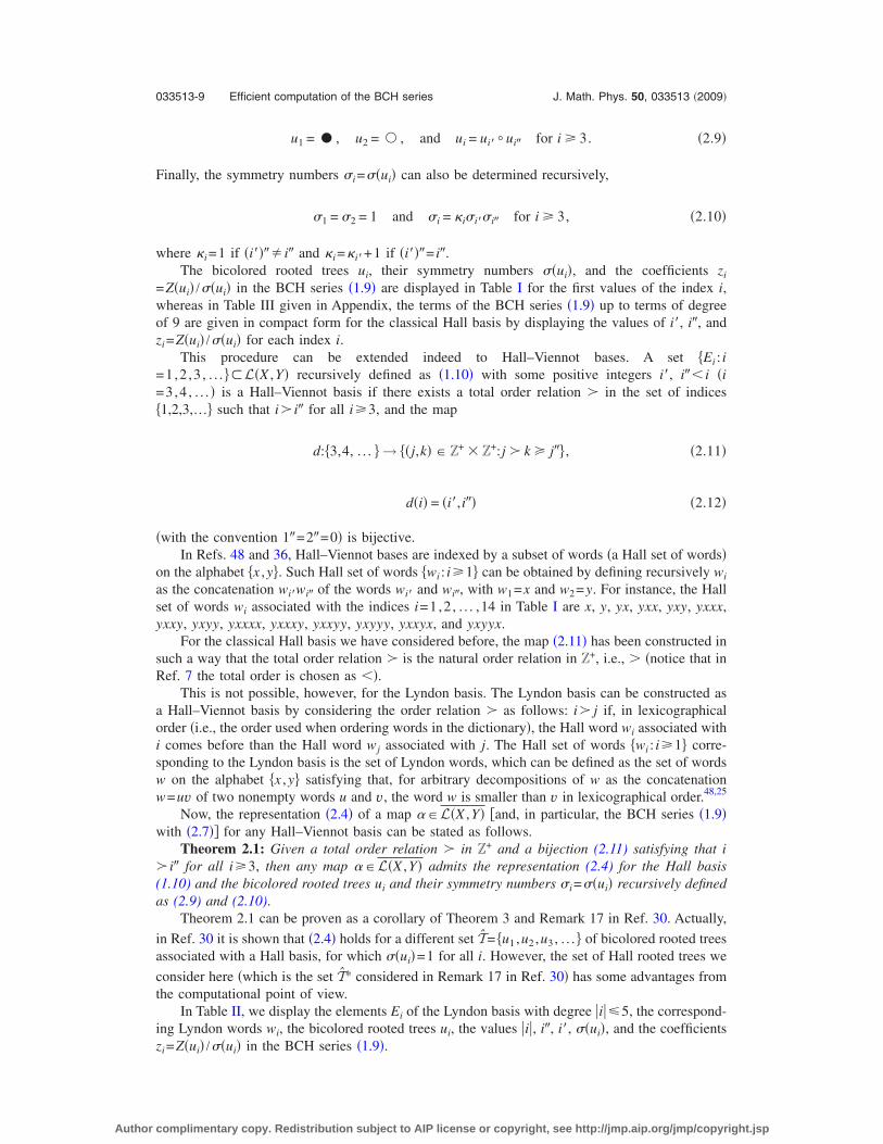
u1 = � , u2 = � , and ui = ui� � ui� for i � 3. �2.9�

Finally, the symmetry numbers i= �ui� can also be determined recursively,

1 = 2 = 1 and i = �i i� i� for i � 3, �2.10�

where �i=1 if �i�� i� and �i=�i�+1 if �i��= i�.The bicolored rooted trees ui, their symmetry numbers �ui�, and the coefficients zi

=Z�ui� / �ui� in the BCH series �1.9� are displayed in Table I for the first values of the index i,whereas in Table III given in Appendix, the terms of the BCH series �1.9� up to terms of degreeof 9 are given in compact form for the classical Hall basis by displaying the values of i�, i�, andzi=Z�ui� / �ui� for each index i.

This procedure can be extended indeed to Hall–Viennot bases. A set �Ei : i=1,2 ,3 , . . . ��L�X ,Y� recursively defined as �1.10� with some positive integers i�, i�� i �i=3,4 , . . . � is a Hall–Viennot basis if there exists a total order relation � in the set of indices�1,2,3,…� such that i� i� for all i�3, and the map

d:�3,4, . . . � → ��j,k� � Z+ � Z+:j � k � j�� , �2.11�

d�i� = �i�,i�� 2.12�

�with the convention 1�=2�=0� is bijective.In Refs. 48 and 36, Hall–Viennot bases are indexed by a subset of words �a Hall set of words�

on the alphabet �x ,y�. Such Hall set of words �wi : i�1� can be obtained by defining recursively wi

as the concatenation wi�wi� of the words wi� and wi�, with w1=x and w2=y. For instance, the Hallset of words wi associated with the indices i=1,2 , . . . ,14 in Table I are x, y, yx, yxx, yxy, yxxx,yxxy, yxyy, yxxxx, yxxxy, yxxyy, yxyyy, yxxyx, and yxyyx.

For the classical Hall basis we have considered before, the map �2.11� has been constructed insuch a way that the total order relation � is the natural order relation in Z+, i.e., � �notice that inRef. 7 the total order is chosen as ��.

This is not possible, however, for the Lyndon basis. The Lyndon basis can be constructed asa Hall–Viennot basis by considering the order relation � as follows: i� j if, in lexicographicalorder �i.e., the order used when ordering words in the dictionary�, the Hall word wi associated withi comes before than the Hall word wj associated with j. The Hall set of words �wi : i�1� corre-sponding to the Lyndon basis is the set of Lyndon words, which can be defined as the set of wordsw on the alphabet �x ,y� satisfying that, for arbitrary decompositions of w as the concatenationw=uv of two nonempty words u and v, the word w is smaller than v in lexicographical order.48,25

Now, the representation �2.4� of a map �L�X ,Y� �and, in particular, the BCH series �1.9�with �2.7�� for any Hall–Viennot basis can be stated as follows.

Theorem 2.1: Given a total order relation � in Z+ and a bijection (2.11) satisfying that i� i� for all i�3, then any map �L�X ,Y� admits the representation (2.4) for the Hall basis(1.10) and the bicolored rooted trees ui and their symmetry numbers i= �ui� recursively definedas (2.9) and (2.10).

Theorem 2.1 can be proven as a corollary of Theorem 3 and Remark 17 in Ref. 30. Actually,

in Ref. 30 it is shown that �2.4� holds for a different set T̂= �u1 ,u2 ,u3 , . . . � of bicolored rooted treesassociated with a Hall basis, for which �ui�=1 for all i. However, the set of Hall rooted trees we

consider here �which is the set T̂* considered in Remark 17 in Ref. 30� has some advantages fromthe computational point of view.

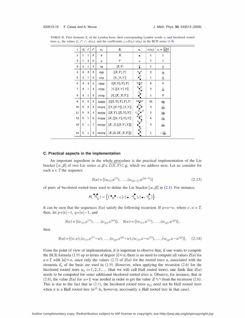
In Table II, we display the elements Ei of the Lyndon basis with degree i�5, the correspond-ing Lyndon words wi, the bicolored rooted trees ui, the values i, i�, i�, �ui�, and the coefficientszi=Z�ui� / �ui� in the BCH series �1.9�.



C. Practical aspects in the implementation

An important ingredient in the whole procedure is the practical implementation of the Liebracket � ,�� of two Lie series ,��L�X ,Y��g, which we address next. Let us consider foreach u�T the sequence

S�u� = ��u�1�,u�1��, . . . ,�u�u−1�,u

�u−1�� 2.13�

of pairs of bicolored rooted trees used to define the Lie bracket � ,�� in �2.1�. For instance,

It can be seen that the sequences S�u� satisfy the following recursion. If u=v �w, where v ,w�T,then, let p= v−1, q= w−1, and

S�v� = ��v�1�,v�1��, . . . ,�v�p�,v

�p��, S�w� = ��w�1�,w�1��, . . . ,�w�q�,w

�q�� ,

then

S�u� = ��w,v�,�v�1�,v�1� � w�, . . . ,�v�p�,v

�p� � w�,�w�1�,v � w�1��, . . . ,�w�q�,v � w�q�� . �2.14�

TABLE II. First elements Ei of the Lyndon basis, their corresponding Lyndon words wi and bicolored rootedtrees ui, the values i, i�, i�, �ui�, and the coefficients zi=Z�ui� / �ui� in the BCH series �1.9�.



The minimal set T̃n of bicolored rooted trees u for which Z�u� needs to be computed in orderto get the values of Z�ui� for Hall rooted trees with i�n by using recursion �2.6� can bedetermined by requiring that

�ui:i � n� � T̃n � T and S�T̃n� � T̃n � T̃n.

It can be seen that the subset T̃n of bicolored rooted trees can be alternatively defined as follows:We say that a bicolored rooted tree v�T is covered by u�T if either v can be obtained from u byremoving some of its vertices and edges or u=v. For instance, the bicolored rooted trees coveredby the tree u11 in Table II are

Then, it can be seen that T̃n is the set of bicolored rooted trees covered by some of the trees in�ui : i�n�.

As a summary of this treatment, we next describe the main steps of the algorithm that we useto compute the BCH series up to terms of a given degree N for an arbitrary Hall–Viennot basis.Let mN be sum of the dimensions of the homogeneous subspaces L�X ,Y�n for 1�n�N and let m̃N

be the number of bicolored rooted trees in T̃N �so that mN� m̃N�. We proceed as follows for a givenN:

�1� Determine the values i� , i� for each i=1, . . . ,mN such that the Ei given by �1.10� are theelements of degree i�N of the required Hall–Viennot basis. Algorithm 1 can be used in thecase of the basis of P. Hall. We use a similar �although slightly more complex� algorithm forthe general case.

�2� Determine the bicolored rooted trees u� T̃N together with the u−1 pairs of bicolored rootedtrees in S�u� recursively obtained by �2.14�. Actually, we associate each bicolored rooted tree

in T̃N with a positive integer, such that T̃N= �ui : i=1,2 , . . . , m̃N� �and �ui : i=1,2 , . . . ,mN� isthe set of Hall trees of degree i�N�. Each S�ui� is then represented as a list of i−1 pairsof positive integers.

�3� Represent the truncated versions of Lie series �truncated up to terms of degree N� as a listof m̃N real values �1 , . . . ,m̃N

� corresponding to ��u1� , . . . ,�um̃N��. The Lie bracket �

= � ,�� of two Lie series can be implemented as a way to obtain the list ��1 , . . . ,�m̃N� from

the lists �1 , . . . ,m̃N� and ��1 , . . . ,�m̃N

� in terms of the pairs of integers representing S�ui�for each i=1, . . . , m̃N.

�4� Represent the truncated versions of BCH series Z �truncated up to terms of degree N� as a listof m̃N rational values �Z1 , . . . ,Zm̃N

� corresponding to �Z�u1� , . . . ,Z�um̃N��, which can be ob-

tained by initializing that list as �1,1,0,…,0� and applying �2.6� repeatedly for n=2, . . . ,N.

It is worth noticing that the number of trees in T̃n is different for different Hall–Viennot bases.

For instance, for the basis of P. Hall, T̃20 has 724 018 bicolored rooted trees, while for the Lyndon

basis the set T̃20 has 1 952 325 bicolored rooted trees. Due to this fact, the amount of memory andCPU time required to compute with our algorithm the BCH formula up to a given degree for theLyndon basis is considerably larger than for the basis of P. Hall. Moreover, the number of nonzerocoefficients zi in the BCH formula differs considerably in both bases. For instance, there are109 697 nonvanishing coefficients zi �out of 111 013 elements Ei of degree i�20� in the BCHformula for the basis of P. Hall, while for the Lyndon basis the number of nonvanishing coeffi-cients zi is 76 760.



III. OPTIMAL CONVERGENCE DOMAIN OF THE BCH SERIES

A. The BCH formula and the Magnus expansion

One particularly simple way of obtaining a sharp bound on the convergence domain for theBCH series consists in relating it with the Magnus expansion for linear differential equations. Forthe sake of completeness, we summarize here the main features of this procedure.

Suppose we have the nonautonomous linear differential equation

dU

dt= A�t�U, U�0� = I , �3.1�

where U�t� and A�t� are operators acting on some Hilbert space H �in particular, n�n real orcomplex matrices�. Then the idea is to express the solution U�t� as the exponential of a certainoperator ��t�,

U�t� = exp ��t� . �3.2�

By substituting �3.2� into �3.1�, one can derive the differential equation satisfied by the exponent�,

�� = �k=0

�Bk

k!ad�

k �A�t��, ��0� = O . �3.3�

By applying Picard’s iteration on �3.3�, one gets an infinite series for ��t�,

��t� = �m=1

�

�m�t� , �3.4�

whose terms can be obtained recursively from

�1�t� = �0

t

A�t1�dt1,

�m�t� = �j=1

m−1Bj

j!�

0

t

�ad��s�A�s��mds, m � 2. �3.5�

Equations �3.2� and �3.4� constitute the so-called Magnus expansion for the solution of �3.1�,whereas the infinite series �3.4� with �3.5� is known as the Magnus series.

Since the 1960s,49 the Magnus expansion has been successfully applied as a perturbative toolin numerous areas of physics and chemistry, from atomic and molecular physics to nuclear mag-netic resonance and quantum electrodynamics �see Refs. 4 and 5 for a review and a list ofreferences�. Also, since the work by Iserles and Nørsett,20 it has been used as a tool to constructpractical algorithms for the numerical integration of Eq. �3.1�, while preserving the main qualita-tive properties of the exact solution.

In general, the Magnus series does not converge unless A is small in a suitable sense, andseveral bounds to the actual radius of convergence have been obtained along the years. Recently,the following theorem has been proven.9

Theorem 3.1: Let us consider the differential equation U�=A�t�U defined in a Hilbert spaceH, dim H��, with U�0�= I, and let A�t� be a bounded linear operator on H. Then, the Magnusseries ��t�=�k=1

� �k�t�, with �k given by (3.5) converges in the interval t� �0,T� such that

�0

T

A�s�ds �



and the sum ��t� satisfies exp ��t�=U�t�. The statement also holds when H is infinite dimensionalif U is a normal operator (in particular, if U is unitary). Here · stands for the norm defined bythe inner product on H.

Moreover, it has been shown that the convergence domain of the Magnus series provided bythis theorem is the best result one can get for a generic bounded operator A�t� in a Hilbert space,in the sense that it is possible to find specific A�t� where the series diverges for any time t such that�0

t A�s�ds�.29,9

Now, given two operators X and Y, let us consider Eq. �3.1� with

A�t� = �Y , 0 � t � 1

X , 1 � t � 2.� �3.6�

Clearly, the exact solution at t=2 is given by U�2�=eXeY. On the other hand, if we apply recur-rence �3.5� to compute U�2� with the Magnus expansion, U�2�=e��2�, we get �1�2�=X+Y andmore generally �n�2�=Zn in �1.4�. In other words, the BCH series can be considered as theMagnus expansion corresponding to the differential equation �3.1� with A�t� given by �3.6� at t=2.

Since �0t=2A�s�ds= X+ Y, Theorem 3.1 leads to the following bound on the convergence

of the BCH series.Theorem 3.2: Let X and Y be two bounded elements in a Hilbert space H with dim H�2.

Then the BCH formula in the form (1.4), i.e., expressed as a series of homogeneous Lie polyno-mials in X and Y, converges when X+ Y�.

Of course, this result can be generalized to any set X1 ,X2 , . . . ,Xk of bounded operators: thecorresponding BCH series is convergent if X1+ ¯ + Xk� in the 2-norm.

Let us illustrate the result provided by Theorem 3.2 with a simple example involving 2�2matrices.

Example 1: Given

X = � 0

0 − , Y = �0 �

0 0 , �3.7�

with ,��C, a simple calculation shows that

log�eXeY� = X +2

1 − e−2Y ,

which is an analytic function for � with first singularities at = � i. Therefore, the BCHformula cannot converge if �, independently of ��0. By taking the spectral norm, it is clearthat X= , Y= �, so that the convergence domain given by Theorem 3.2 is + ��.Notice that in the limit �→0 this domain is optimal. �

Generally speaking, however, the bound given by Theorem 3.2 is conservative, i.e., the BCHseries converges for larger values of X and Y. Thus, in the previous example, for any and �with � and + ��, the BCH series also converges. One would like therefore to have amore realistic characterization of this feature. It turns out that this is indeed feasible for complexn�n matrices.

B. Convergence for matrices

1. Convergence determined by the eigenvalues

For complex n�n matrices it is possible to use the theory of analytic matrix functions andmore specifically, the logarithm of an analytic matrix function, in a similar way as in the Magnusexpansion,9 to characterize more precisely the convergence of the BCH series.

To begin with, let us introduce a parameter ��C and consider the substitution�X ,Y�� X ,�Y� into Eq. �1.1�. It is clear that



U�� e�Xe�Y

is an analytic function of �, det U��0 and the matrix function Z��=log U�� is also analytic at�=0. Equivalently, the series Z�� is convergent for sufficiently small �. It turns out that the actualradius of convergence of this series is related with the existence of multiple eigenvalues of U��.Let us denote by �1�� , . . . ,�n�� the eigenvalues of the matrix U��. Observe that U�0�= I, so that�1�0�= ¯ =�n�0�=1, and we can take the principal values of the logarithm, log �1�0�= ¯

=log �n�0�=0. In essence, if the analytic matrix function U�� has an eigenvalue �0��0� of mul-tiplicity l�1 for a certain �0 such that �a� there is a curve in the �-plane joining �=0 with �=�0, and �b� the number of equal terms in log �1��0�, log �2��0� , . . . , log �l��0� such that �k��0�=�0, k=1, . . . , l is less than the maximum dimension of the elementary Jordan block correspond-ing to �0, then the radius of convergence of the series Z��=�k�1�kZk verifying exp Z��=U�� isprecisely r= �0.9

More specifically, we find first the values of the parameter � for which the characteristicpolynomial det�U��−�I� has multiple roots and write them in order of nondecreasing absolutevalue,

�0�1�,�0

�2�,�0�3�, . . . . �3.8�

Next, we consider the circle �= �0�1� in the complex �-plane and denote by �0

�1� an eigenvalue ofU��0

�1�� with multiplicity l1�1. Let � move along some fixed curve L from �=0 to �=�0�1� in the

circle �� 0�1�. Then it is clear that l1 eigenvalues � j�� will tend to �0

�1� at �=�0�1�. If these points

lie at �=�0�1� on the same sheet of the Riemann surface of the function log z, and this is true for all

�possible� multiple eigenvalues of U�� at �=�0�1�, then �0

�1� is called a extraneous root. Otherwise,�0

�1� is called a nonextraneous root.By the analysis carried out in Ref. 51, when �� 0

�1� the numbers log � j�� are uniquelydetermined as eigenvalues of the matrix Z�� and this series is convergent. This is also true at�= �0

�1� if �0�1� is an extraneous root, since then the eigenvalues of Z�� retain their identity

throughout the collision process, so that we proceed to the next value in the sequence �3.8� untila nonextraneous root is obtained.

Assume, for simplicity, that �0�2� is the first nonextraneous root, for which there exists an

eigenvalue �0 of U�� with multiplicity l�1. Associated with this multiple eigenvalue �0 there isa pair of integers �p ,q� defined as follows.

The integer p is the greatest number of equal terms in the set of numbers log �1��0�,log �2��0� , . . . , log �l��0� such that �k��0�=�0, k=1, . . . , l.

The integer q is the maximum degree of the elementary divisors ��−�0�k of U��0�, i.e., themaximum dimension of the elementary Jordan block corresponding to �0.

Under these conditions, it has been proven that if p�q for the eigenvalue �0, then the radiusof convergence of the series Z��=�k�1�kZk is precisely r= �0.51

Although in some cases with p�q the series Z�� may converge at �= �0 and the radius ofconvergence r is greater than �0 �for instance, when X and Y are diagonal�, this situation isexceptional in a topological sense, as explained in Ref. 51, pp. 65 and 66.

2. Examples

In order to illustrate this result we next consider a pair of examples involving also 2�2matrices.

Example 1: The first example involves again the matrices X and Y given by �3.7�. In this case

U�� = e�Xe�Y = �e� ��e�

0 e−� .

The first values of � for which there are multiple eigenvalues of U�� are



� = 0, � = � i

.

The first value, �=0, is clearly an extraneous root, whereas the eigenvalues of the matrix U��move along the unit circle, one clockwise and the other counterclockwise from

�1,2�0� = 1 to �1,2�i/� = − 1

when � varies along the imaginary axis from �=0 to �= i / �the same considerations apply tothe case �=−i /�. Then, obviously, p=1 and q=2, so that the radius of convergence of the seriesZ�� is

� =

.

By fixing �=1, we get the actual domain of convergence of the BCH series as =, i.e., thesame result as in Sec. III A �

Example 2: Consider now the matrices

A = �0 0

1 0 , B = �0 1

0 0 ,

and X=A, Y =B, with �0. Then

U�� = � 1 �

� 1 + 2�2 �3.9�

has multiple eigenvalues when �0�1�=0, �0

�2�= � i2 /. As � varies along the imaginary axis from�=0 to �=�0

�2�, the eigenvalues of the matrix U��,

�1,2�� = 1 +2

2�2 ��1 +

2

2�2 2

− 1,

move along the unit circle, one clockwise and the other counterclockwise from

�1,2�0� = 1 to �1,2��0�2�� = − 1.

Thus, �1��0�2�� and �2��0

�2�� lie on different sheets of the Riemann surface of the function log z andtherefore �0

�2� is a nonextraneous root, with p=1. Since U��0�2��−I, we have q=2, so that the

radius of convergence of the series Z�� is precisely

r = �0�2� =

2

. �3.10�

This result should be compared with the bound provided by the Magnus expansion. Since A= B=1, Theorem 3.2 guarantees the convergence of the BCH series in this case whenever2�� or �� /2, which, in view of �3.10�, is clearly a conservative estimate.

We can also check numerically the rate of convergence of the BCH series in this example asa function of the parameter �. Let us denote by Z�N� the sum of the first N terms of the series, i.e.,

Z�N�� = �n=1

N

Zn��

and compute, for =2 and different values of �, the matrix



Er�� = U��e−Z�N�� − I ,

where U�� is given by �3.9�. If � belongs to the convergence domain of the BCH series for thematrices X and Y �i.e., ��1�, then Er��→0 as N→�.

First we take �= 14 . With N=10, the elements of Er are of order of 10−7, whereas adding five

additional terms in the series, N=15, the elements of Er are approximately 10−10.Next we choose �=0.9, i.e., a value near the boundary of the convergence domain. In this case

with N=15 the convergence of the series does not manifest at all. In fact, a much larger numberof terms is required to achieve significant results. Thus, for the elements of Er to be of order of10−8 we need to compute N=150 terms of the BCH series, whereas with N=200 the elements ofEr are of order of 10−10. The computations have been carried out with the recurrence �1.8�. �

As this example clearly shows, it is not always possible to determine accurately the conver-gence domain of the BCH series by computing successive approximations, since the rate ofconvergence can be slow indeed near the boundary. For this reason it could be of interest to designa procedure to apply in practice the characterization of the convergence in terms of the eigenval-ues of the matrix U�� analyzed in Sec. III B 1 for matrices.

This procedure could be as follows. Given two matrices X, Y, take the product of exponentials

U�� = e�Xe�Y

with �=rei�. Next, define a grid in the �-plane, for instance, in polar coordinates �r ,��, by �r=rf / �n+1�, ��=2 / �m+1� for two integers n, m�1 and a sufficiently large value rf �1. Then,for each point in the grid �rk=k�r, �l= l��, k=1, . . . ,n+1, l=0,1 , . . . ,m, compute the corre-sponding matrix U�� and its eigenstructure, locating where there are multiple eigenvalues �withina prescribed tolerance�. If some of these multiple eigenvalues have a negative real part, thereexists a point in the neighborhood where the conditions enumerated in Sec. III B 1 are satisfied,and therefore we have approximately located the value of � where the BCH series fails to con-verge. This approximation can be made more accurate by applying, for instance, Newton’smethod. The actual radius of convergence will be given by the smallest number r found in thisway. Finally, if r�1, then obviously the BCH series corresponding to X and Y converges.

IV. SOME APPLICATIONS

As an illustration of the usefulness of the previous results, in this section we present two notso trivial applications of the formalism developed in Sec. II for constructing explicitly the BCHseries up to arbitrarily high order.

A. The symmetric BCH formula

Sometimes it is necessary to compute the Lie series W defined by

exp� 12X�exp�Y�exp� 1

2X� = exp�W� . �4.1�

This occurs, for instance, if one is interested in obtaining the order conditions satisfied by time-symmetric composition methods for the numerical integration of differential equations.52,39 Twoapplications of the usual BCH formula give then the expression of W in the Hall basis of L�X ,Y�.

A more efficient procedure is obtained, however, by introducing a parameter � in �4.1� suchthat

W�� = log�e�X/2eYe�X/2� �4.2�

and deriving the differential equation satisfied by W��. From the derivative of the exponentialmap, one gets



dW

d�= X + �

n=2

�Bn

n!adW

n X, W�0� = Y , �4.3�

whence it is possible to construct explicitly W as the series W��=�k=0� Wk��, with

W1�� = X� + Y ,

W2�� = 0,

Wl�� = �j=2

l−1Bj

j!�

0

�

�adWj X�lds, l � 3, �4.4�

where, in general, W2m=0 for m�1. By following a similar approach as with Eq. �1.8� in the usualBCH series in Sec. II, the recursion �4.4� allows one to express W in �4.1� as

W = �i�1

wiEi. �4.5�

The coefficients wi of this series up to degree of 9 in the classical Hall basis are collected in TableIV in Appendix. As with the usual BCH series, the coefficients up to degree of 19 in both Hall andLyndon bases can be found at www.gicas.uji.es/research/bch.html.

With respect to the convergence of the series, theorem �3.2� guarantees that W is convergentat least when X+ Y�.

B. The BCH formula and a problem of Thompson

In a series of papers,43,32,44,45 Thompson considered the problem of constructing a represen-tation of the BCH formula as

eXeY = eZ, with Z = SXS−1 + TYT−1, �4.6�

for certain functions S=S�X ,Y� and T=T�X ,Y� depending on X and Y. By using analytic tech-niques related with the Kashiwara–Vergne method, Rouvière38 proved that a Lie series ��X ,Y�exists such that

S = e��X,Y�, T = e��−Y,−X� �4.7�

and converges when X, Y are replaced by normed elements near 0, whereas the representation�4.6� is global when both X and Y are skew-Hermitian matrices.43

Thompson himself developed a computational technique for constructing explicitly the series��X ,Y� up to terms of degree of 10. Although his results were not published, he pointed out thatthey furnished strong evidence of the convergence of the series ��X ,Y� on the closed unit spherein any norm for which �X ,Y�� XY.45

With the aim of clarifying this issue and illustrating the techniques developed in Sec. II, weproceed next to compute ��X ,Y�. Since ��X ,Y��L�X ,Y�, i.e., is a Lie series, it can be written as

��X,Y� = �i�1

�iEi,

where the elements Ei have been introduced in �1.9�, and the goal is to determine the coefficients�i. This can be accomplished as follows. From the well known formula eUVe−U=eadUV, it is clearthat



Z = ead��X,Y�X + ead��−Y,−X�Y . �4.8�

Next we expand ead��X,Y�X and ead��−Y,−X�Y into infinite series as a linear combination of the Hallbasis in L�X ,Y� and match the resulting terms with the corresponding to the BCH series for Z.Then a recursive system of equations is obtained for the coefficients �i.

It is, in fact, possible to get a closed expression for ��X ,Y� up to terms Y2 by taking intoaccount the corresponding formula of Z.34 Specifically, from

Z = X +adX

1 − e−adXY mod Y2, �4.9�

a simple calculation leads to

��X,Y� = f�adX�Y mod Y2,

with the function f�z� given by

f�z� =ez

1 − ez +1

zez/4 = −

1

4−

5

96z +

1

384z2 +

143

92 160z3 +

1

122 880z4 + ¯ . �4.10�

Working in the classical Hall basis, the complete expression up to degree of 4 reads

f�z� = − 14Y + 5

96�Y,X� + 1384��Y,X�,X� + 11

768��Y,X�,Y� − 14392 160��Y,X�,X�,X� − 283

92 160��Y,X�,X�,Y�

+ 1123 040��Y,X�,Y�,Y� ,

i.e., the corresponding equations have a unique solution. This is not the case, however, at degreeof 5, where a free parameter appears, which can be chosen to be �10. Then

�12 =− 137 − 184 320�10

184 320, �13 =

− 511 − 737 280�10

737 280.

As a matter of fact, if higher degrees are considered, more and more free parameters appear in thecorresponding solution. Thus, at degree of 7 there are two additional parameters �for instance, �26

and �30�, whereas at degree of 8 �50 and �52 can be chosen as free parameters. We conclude,therefore, that there are infinite solutions to the problem posed by Thompson depending on anincreasing number of free parameters. An interesting issue would be to determine the value ofthese parameters in order to render the whole series convergent on a domain as large as possible.

C. Distribution of coefficients in the Lyndon basis

As we previously mentioned, there are noteworthy differences in the results obtained when thealgorithm of Sec. II is applied to the BCH series in the classical Hall basis and the Lyndon basis,particularly with respect to the number of vanishing coefficients. In the basis of P. Hall there are1316 zero coefficients out of 111 013 up to degree m=20, whereas in the Lyndon basis the numberof vanishing terms rises to 34 253 �more than 30% of the total number of coefficients�.

More remarkably, one notices that the distribution of these vanishing coefficients in the Lyn-don basis follows a very specific pattern. Before entering into the details, let us denote forsimplicity Lm�L�X ,Y�m. We first remark that, for each m�2, the Lyndon basis Bm of Lm is adisjoint union Bm=Bm,1�Bm,2 with Bm,2= �X ,Bm−1�. Thus, Lm=Lm,1 � Lm,2, where Lm,2

= �X ,Lm−1�, and Bm,k �k=1,2� is a basis of Lm,k. In particular, adXm−1 Y �Bm. In this sense, from

our computations we make two observations. First, the coefficient in the BCH formula of theelement adX

m−1 Y in the basis Bm is 0 for even m. Second, the coefficients for the terms in Bm,1 arealso zero for even m. This gives a total number of



nc�2p� = dim�L2p� − dim�L2p−1� + 1, p � 2,

vanishing coefficients of terms of degree m=2p in the BCH formula written in the Lyndon basis.Thus, for instance, when p=10, the number of total number of vanishing coefficients is nc�20�=dim�L20�−dim�L19�+1=52 377−27 594+1=24 784.

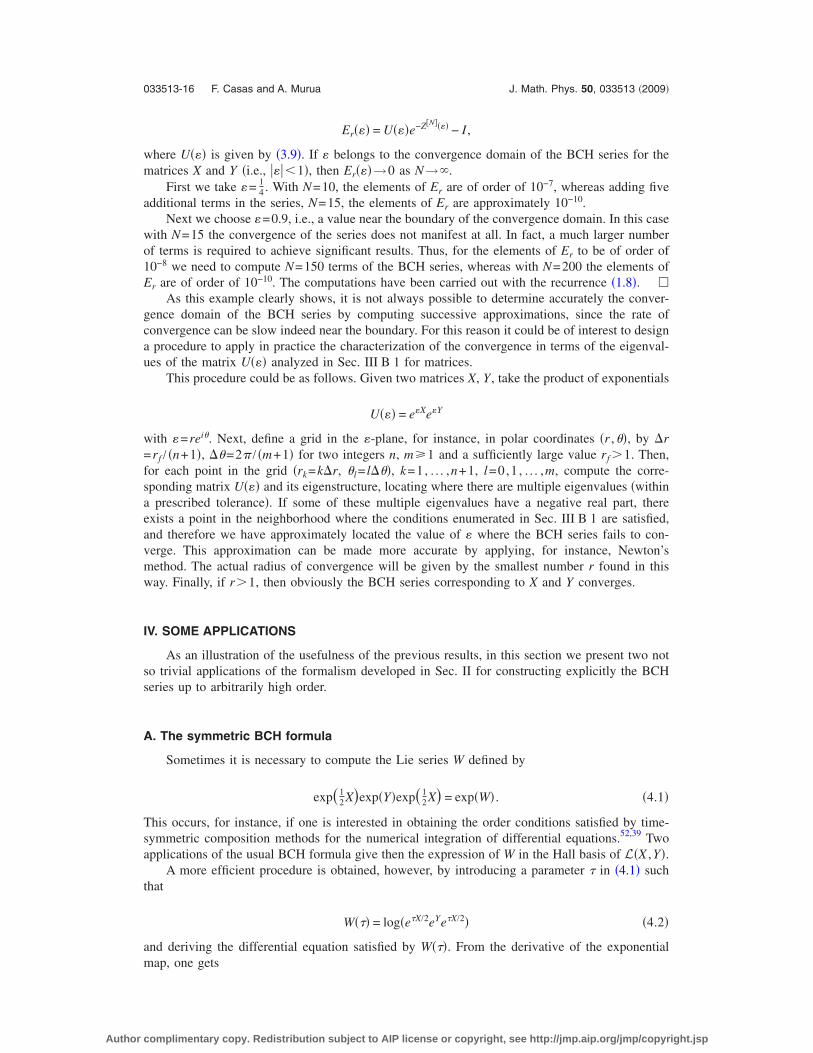
TABLE III. Table of values of i� and i� for i�3 in �1.10� for the classical Hall basis and the values zi�Q in the BCHformula �1.9�.

i i� i� zi i i� i� zi i i� i� zi

1 1 0 1 44 25 2 1 /10 080 87 31 3 −11 /30 240

2 2 0 1 45 26 2 23 /120 960 88 32 3 −19 /100 800

3 2 1 −1 /2 46 27 2 1 /10 080 89 33 3 −1 /43 200

4 3 1 1 /12 47 28 2 1 /60 480 90 34 3 −1 /10 080

5 3 2 −1 /12 48 29 2 0 91 35 3 −1 /50 400

6 4 1 0 49 15 3 0 92 15 4 −1 /33 600

7 4 2 1 /24 50 16 3 1 /40 032 93 16 4 −13 /120 960

8 5 2 0 51 17 3 23 /30 240 94 17 4 −1 /10 080

9 6 1 −1 /720 52 18 3 1 /2 240 95 18 4 −11 /201 600

10 6 2 −1 /180 53 19 3 1 /15 120 96 19 4 −1 /43 200

11 7 2 1 /180 54 20 3 0 97 20 4 −1 /7 560

12 8 2 1 /720 55 21 3 1 /2 250 98 21 4 −1 /10 080

13 4 3 −1 /120 56 22 3 1 /10 080 99 22 4 1 /50 400

14 5 3 −1 /360 57 9 4 0 100 23 4 1 /20 160

15 9 1 0 58 10 4 1 /10 080 101 15 5 −23 /302 400

16 9 2 −1 /1 440 59 11 4 −1 /20 160 102 16 5 −1 /5 760

17 10 2 −1 /360 60 12 4 −1 /20 160 103 17 5 13 /151 200

18 11 2 −1 /1 440 61 13 4 0 104 18 5 19 /120 960

19 12 2 0 62 14 4 −1 /2 520 105 19 5 1 /33 600

20 6 3 0 63 9 5 1 /4 032 106 20 5 −13 /30 240

21 7 3 −1 /240 64 10 5 1 /840 107 21 5 −23 /100 800

22 8 3 −1 /720 65 11 5 1 /1 440 108 22 5 −1 /100 800

23 5 4 1 /240 66 12 5 1 /12 096 109 23 5 −1 /33 600

24 15 1 1 /30 240 67 13 5 1 /1 260 110 9 6 −1 /60 480

25 15 2 1 /5 040 68 14 5 1 /10 080 111 10 6 −1 /90 720

26 16 2 1 /3 780 69 7 6 −1 /10 080 112 11 6 1 /30 240

27 17 2 −1 /3 780 70 8 6 −13 /30 240 113 12 6 −11 /302 400

28 18 2 −1 /5 040 71 8 7 −1 /3 360 114 13 6 1 /15 120

29 19 2 −1 /30 240 72 42 1 −1 /1 209 600 115 14 6 1 /3 780

30 9 3 1 /2 016 73 42 2 −1 /151 200 116 9 7 −11 /120 960

31 10 3 23 /15 120 74 43 2 −1 /56 700 117 10 7 −1 /6 720

32 11 3 1 /5 040 75 44 2 −1 /75 600 118 11 7 −1 /14 400

33 12 3 −1 /10 080 76 45 2 1 /75 600 119 12 7 −11 /120 960

34 13 3 1 /1 260 77 46 2 1 /56 700 120 13 7 −1 /20 160

35 14 3 1 /5 040 78 47 2 1 /151 200 121 14 7 17 /100 800

36 6 4 1 /5 040 79 48 2 1 /1 209 600 122 9 8 −1 /20 160

37 7 4 −1 /10 080 80 24 3 −1 /43 200 123 10 8 17 /151 200

38 8 4 1 /1 680 81 25 3 −37 /302 400 124 11 8 1 /6 048

39 6 5 13 /15 120 82 26 3 −11 /60 480 125 12 8 1 /60 480

40 7 5 −1 /1 120 83 27 3 −11 /302 400 126 13 8 −1 /100 800

41 8 5 −1 /5 040 84 28 3 11 /302 400 127 14 8 1 /37 800

42 24 1 0 85 29 3 1 /100 800

43 24 2 1 /60 480 86 30 3 −1 /7 560



With these considerations in mind, we can proceed next to explain the observed phenomena.First, notice that expression �4.9� gives explicitly the last term of the BCH series in the Lyndonbasis at each degree. By formally expanding in power series of adX we get

TABLE IV. Table of values of i� and i� for i�3 in �1.10� for the classical Hall basis and the values wi�Q in the symmetricBCH formula �4.1�

i i� i� wi i i� i� wi i i� i� wi

1 1 0 1 44 25 2 0 87 31 3 1 /4 608

2 2 0 1 45 26 2 0 88 32 3 23 /134 400

3 2 1 0 46 27 2 0 89 33 3 1 /37 800

4 3 1 −1 /24 47 28 2 0 90 34 3 1 /23 040

5 3 2 −1 /12 48 29 2 0 91 35 3 1 /201 600

6 4 1 0 49 15 3 0 92 15 4 193 /6 451 200

7 4 2 0 50 16 3 0 93 16 4 53 /483 840

8 5 2 0 51 17 3 0 94 17 4 25 /193 536

9 6 1 7 /5 760 52 18 3 0 95 18 4 1 /22 400

10 6 2 7 /1 440 53 19 3 0 96 19 4 −13 /1 209 600

11 7 2 1 /180 54 20 3 0 97 20 4 53 /483 840

12 8 2 1 /720 55 21 3 0 98 21 4 17 /161 280

13 4 3 1 /480 56 22 3 0 99 22 4 −3 /44 800

14 5 3 −1 /360 57 9 4 0 100 23 4 −19 /322 560

15 9 1 0 58 10 4 0 101 15 5 367 /4 838 400

16 9 2 0 59 11 4 0 102 16 5 193 /645 120

17 10 2 0 60 12 4 0 103 17 5 247 /604 800

18 11 2 0 61 13 4 0 104 18 5 53 /241 920

19 12 2 0 62 14 4 0 105 19 5 1 /33 600

20 6 3 0 63 9 5 0 106 20 5 53 /161 280

21 7 3 0 64 10 5 0 107 21 5 193 /403 200

22 8 3 0 65 11 5 0 108 22 5 13 /201 600

23 5 4 0 66 12 5 0 109 23 5 −1 /5 600

24 15 1 −31 /967 680 67 13 5 0 110 9 6 11 /774 114

25 15 2 −31 /161 280 68 14 5 0 111 10 6 1 /290 304

26 16 2 −13 /30 240 69 7 6 0 112 11 6 −1 /15 360

27 17 2 −53 /120 960 70 8 6 0 113 12 6 −89 /1 209 600

28 18 2 −1 /5 040 71 8 7 0 114 13 6 −11 /241 920

29 19 2 −1 /30 240 72 42 1 127 /154 828 800 115 14 6 −13 /80 640

30 9 3 −53 /161 280 73 42 2 127 /19 353 600 116 9 7 1 /12 096

31 10 3 −11 /12 096 74 43 2 157 /7 257 600 117 10 7 11 /64 512

32 11 3 −3 /4 480 75 44 2 367 /9 676 800 118 11 7 1 /33 600

33 12 3 −1 /10 080 76 45 2 23 /604 800 119 12 7 −11 /120 960

34 13 3 −1 /4 032 77 46 2 79 /3 628 800 120 13 7 1 /35 840

35 14 3 −1 /6 720 78 47 2 1 /151 200 121 14 7 −29 /134 400

36 6 4 −19 /80 640 79 48 2 1 /1 209 600 122 9 8 211 /1 935 360

37 7 4 −1 /10 080 80 24 3 367 /19 353 600 123 10 8 173 /604 800

38 8 4 17 /40 320 81 25 3 473 /4 838 400 124 11 8 5 /24 192

39 6 5 −53 /60 480 82 26 3 41 /215 040 125 12 8 1 /60 480

40 7 5 −19 /13 440 83 27 3 211 /1 209 600 126 13 8 61 /403 200

41 8 5 −1 /5 040 84 28 3 89 /1 209 600 127 14 8 −1 /151 200

42 24 1 0 85 29 3 1 /100 800

43 24 2 0 86 30 3 79 /967 680



Z = X + Y +1

2adX Y + �

k=2

�

�− 1�kBk

k!adX

k Y mod Y2.

Since B2n+1=0 for all n�1, the coefficient of adXk Y is nonvanishing only for even values of k, or

equivalently, for odd values of the degree m.As for the remaining zero coefficients, let us consider at this point the symmetric BCH

formula �4.1� again. Clearly the series �4.5� only contains terms of odd degree, i.e., W=�i�0W2i+1, where Wi�Li. By denoting P=X /2 and forming the compositionexp�P�exp�W�exp�−P� one gets trivially

ePeWe−P = eXeY = eZ,

i.e., the standard BCH formula. In the terminology of dynamical systems, exp�W� and exp�Z� aresaid to be conjugated. Alternatively, we can write exp�Z�=exp�adP�exp�W�, so that Z=exp�adP�W. It is worth to write explicitly this relation for each term Zm�Lm of the series Z=�m�0Zm by separating the odd and even degree cases. Specifically,

Z2p+1 = W2p+1 + �j=1

p1

��2j�!�22j adX2j W2p−2j+1,

Z2p = �j=1

p1

��2j − 1�!�22j−1adX2j−1 W2p−2j+1.

From these expressions, it is clear that Z2p+1 contains terms in the whole subspace L2p+1,1

� L2p+1,2 �due to the presence of W2p+1�, whereas Z2p belongs to the subspace L2p,2, whosedimension is equal to dim�L2p−1�. In other words, the remaining dim�L2p�−dim�L2p−1� mustnecessarily vanish. In this sense, the Lyndon basis seems the natural choice to get systematicallythe BCH series with the minimum number of terms. Nevertheless, compared to the basis of P.Hall, more CPU time and memory are required to compute the BCH with our algorithm in theLyndon basis. In particular, 1.5 Gbytes are required to compute the BCH formula up to degree of20 in the Hall basis, whereas 3.6 Gbytes of memory are needed in the Lyndon basis.

V. CONCLUDING REMARKS

The effective computation of the BCH series has a long history and is closely related with themore general problem of carrying out symbolic computations in free Lie algebras. In this work wehave presented a new algorithm which allows us to get a closed expression of the series Z=log�eXeY� up to degree of 20 in terms of an arbitrary Hall–Viennot basis of the free Lie algebragenerated by X and Y, L�X ,Y�, requiring reasonable computational resources. As far as we know,no other results are available up to this degree in terms of a basis of L�X ,Y�. The algorithm isbased on some more general results presented in Ref. 30 on the connection of labeled rooted treeswith an arbitrary Hall–Viennot basis of the free Lie algebra.

We have carried out explicitly the computations to get the coefficients of the BCH series interms of both the classical Hall basis and the Lyndon basis, with some noteworthy differences inthe corresponding results, as analyzed in Sec. IV C.

We have also addressed the problem of the convergence of the series when X and Y arereplaced by normed elements. In the particular case of X and Y being matrices, we have provideda characterization of the convergence in terms of the eigenvalues of eZ.

Although here we have considered only the BCH series, it is clear that other more involvedcalculations can be done, as is illustrated, for instance, by the problem of Thompson studied inSec. IV B. As a matter of fact, we intend to develop a general purpose package to carry outsymbolic computations in a free Lie algebra generated by more than two operators.



ACKNOWLEDGMENTS

The authors would like to thank Professor Xavier Viennot for his very illuminating commentson the observed pattern of zero coefficients in the Lyndon basis. This work has been partiallysupported by Ministerio de Educación y Ciencia �Spain� under Project No. MTM2007-61572�cofinanced by the ERDF of the European Union� and Fundació Bancaixa. The SGI/IZO-SGIkerUPV/EHU �supported by the National Program for the Promotion of Human Resources within theNational Plan of Scientific Research, Development and Innovation-Fondo Social Europeo, MCyT,and Basque Government� is also gratefully acknowledged for generous allocation of resources forour computations in the Lyndon basis.

APPENDIX: COEFFICIENTS OF THE BCH FORMULA

In Table III we collect the indices i� and i� for i�3 in �1.10� for the classical Hall basis andthe values of the coefficients zi in the BCH formula �1.9� up to degree of 9, whereas in Table IVwe gather the corresponding coefficients for the symmetric BCH formula �4.1�.

1 Abramowitz, M. and Stegun, I. A., Handbook of Mathematical Functions �Dover, New York, 1965�.2 Baker, H. F., “Alternant and continuous groups,” Proc. London Math. Soc. 3, 24 �1905�.3 Blanes, S. and Casas, F., “On the convergence and optimization of the Baker–Campbell-Hausdorff formula,” LinearAlgebr. Appl. 378, 135 �2004�.

4 Blanes, S., Casas, F., Oteo, J. A., and Ros, J., “Magnus and Fer expansions for matrix differential equations: theconvergence problem,” J. Phys. A 22, 259 �1998�.

5 Blanes, S., Casas, F., Oteo, J. A., and Ros, J., “The Magnus expansion and some of its applications,” Phys. Rep. 470, 151�2009�.

6 Bose, A., “Dynkin’s method of computing the terms of the Baker-Campbell-Hausdorff series,” J. Math. Phys. 30, 2035�1989�.

7 Bourbaki, N., Lie Groups and Lie Algebras �Springer, New York, 1989�, Chaps. 1–3.8 Campbell, J. E., “On a law of combination of operators,” Proc. London Math. Soc. 29, 14 �1898�.9 Casas, F., “Sufficient conditions for the convergence of the Magnus expansion,” J. Phys. A: Math. Theor. 40, 15001�2007�.

10 Dragt, A. J. and Finn, J. M., “Lie series and invariant functions for analytic symplectic maps,” J. Math. Phys. 17, 2215�1976�.

11 Dür, A., Mobius functions, Incidence Algebras and Power-Series Representations, LNM Vol. 1202 �Springer-Verlag,Berlin, 1986�.

12 Dynkin, E. B., “Evaluation of the coefficients of the Campbell-Hausdorff formula,” Dokl. Akad. Nauk SSSR 57, 323�1947�.

13 Goldberg, K., “The formal power series for log�exey�,” Duke Math. J. 23, 13 �1956�.14 Gorbatsevich, V. V., Onishchik, A. L., and Vinberg, E. B., Foundations of Lie Theory and Lie Transformation Groups

�Springer, New York, 1997�.15 Grossman, R. and Larson, R. G., “Hopf-algebraic structure of families of trees,” J. Algebra 126, 184 �1989�.16 Hairer, E., Lubich, Ch., and Wanner, G., Geometric Numerical Integration. Structure-Preserving Algorithms for Ordi-

nary Differential Equations, 2nd ed. �Springer-Verlag, Berlin, 2006�.17 Hausdorff, F., “Die symbolische exponential formel in der gruppen theorie,” Ber. Verh. Saechs. Akad. Wiss. Leipzig,

Math.-Phys. Kl. 58, 19 �1906�.18 Hoffman, M. E., “Combinatorics of rooted trees and Hopf algebras,” Trans. Am. Math. Soc. 355, 3795 �2003�.19 Iserles, A., Munthe-Kaas, H. Z., Nørsett, S. P., and Zanna, A., “Lie-group methods,” Acta Numerica 9, 215 �2000�.20 Iserles, A. and Nørsett, S. P., “On the solution of linear differential equations in Lie groups,” Philos. Trans. R. Soc.

London, Ser. A 357, 983 �1999�.21 Jacobson, N., Lie Algebras �Dover, New York, 1979�.22 Kolsrud, M., “Maximal reductions in the Baker-Hausdorff formula,” J. Math. Phys. 34, 270 �1993�.23 Koseleff, P.-V., “Calcul formel pour les méthodes de Lie en mécanique Hamiltonienne,” Ph.D. thesis, École Polytech-

nique, 1993.24 Kumar, K., “On expanding the exponential,” J. Math. Phys. 6, 1928 �1965�.25 Lothaire, M., Combinatorics on Words �Addison-Wesley, Reading, 1983�.26 Magnus, W., “On the exponential solution of differential equations for a linear operator,” Commun. Pure Appl. Math. 7,

649 �1954�.27 McLachlan, R. I. and Quispel, R., “Splitting methods,” Acta Numerica 11, 341 �2002�.28 Michel, J., “Bases des algèbres de Lie et série de Hausdorff,” Séminaire Dubreil. Algèbre 27, 1 �1974�.29 Moan, P. C., “On backward error analysis and Nekhoroshev stability in the numerical analysis of conservative systems

of ODEs,” Ph.D. thesis, University of Cambridge, 2002.30 Murua, A., “The Hopf algebra of rooted trees, free Lie algebras, and Lie series,” Found Comput. Math. 6, 387 �2006�.31 Newman, M., So, W., and Thompson, R. C., “Convergence domains for the Campbell-Baker-Hausdorff formula,” Linear

Multilinear Algebra 24, 301 �1989�.



http://dx.doi.org/10.1112/plms/s2-3.1.24

http://dx.doi.org/10.1016/j.laa.2003.09.010

http://dx.doi.org/10.1016/j.laa.2003.09.010

http://dx.doi.org/10.1088/0305-4470/31/1/023

http://dx.doi.org/10.1063/1.528242

http://dx.doi.org/10.1063/1.522868

http://dx.doi.org/10.1215/S0012-7094-56-02302-X

http://dx.doi.org/10.1090/S0002-9947-03-03317-8

http://dx.doi.org/10.1098/rsta.1999.0362

http://dx.doi.org/10.1098/rsta.1999.0362

http://dx.doi.org/10.1063/1.530381

http://dx.doi.org/10.1063/1.1704742

http://dx.doi.org/10.1002/cpa.3160070404

32 Newman, M. and Thompson, R. C., “Numerical values of Goldberg’s coefficients in the series for log�exey�,” Math.Comput. 48, 265 �1987�.

33 Oteo, J. A., “The Baker-Campbell-Hausdorff formula and nested commutator identities,” J. Math. Phys. 32, 419 �1991�.34 Postnikov, M., Lie Groups and Lie Algebras. Semester V of Lectures in Geometry �URSS Publishers, Moscow, 1994�.35 Reinsch, M. W., “A simple expression for the terms in the Baker-Campbell-Hausdorff series,” J. Math. Phys. 41, 2434

�2000�.36 Reutenauer, C., Free Lie Algebras �Oxford University Press, Oxford, 1993�.37 Richtmyer, R. D. and Greenspan, S., “Expansion of the Campbell–Baker–Hausdorff formula by computer,” Commun.

Pure Appl. Math. 18, 107 �1965�.38 Rouvière, F., “Espaces symétriques et méthode de Kashiwara–Vergne,” Ann. Sci. Ec. Normale Super. 19, 553 �1986�.39 Sanz-Serna, J. M. and Calvo, M. P., Numerical Hamiltonian Problems �Chapman and Hall, London, 1994�.40 Sornborger, A. T. and Stewart, E. D., “Higher-order methods for simulations on quantum computers,” Phys. Rev. A 60,

1956 �1999�.41 Suzuki, M., “On the convergence of exponential operators—the Zassenhaus formula, BCH formula and systematic

approximants,” Commun. Math. Phys. 57, 193 �1977�.42 Thompson, R. C., “Cyclic relations and the Goldberg coefficients in the Campbell-Baker-Hausdorff formula,” Proc. Am.

Math. Soc. 86, 12 �1982�.43 Thompson, R. C., “Proof of a conjectured exponential formula,” Linear Multilinear Algebra 19, 187 �1986�.44 Thompson, R. C., “Special cases of a matrix exponential formula,” Linear Algebr. Appl. 107, 283 �1988�.45 Thompson, R. C., “Convergence proof for Goldberg’s exponential series,” Linear Algebr. Appl. 121, 3 �1989�.46 Torres-Torriti, M. and Michalska, H., “A software package for Lie algebraic computations,” SIAM Rev. 47, 722 �2005�.47 Varadarajan, V. S., Lie Groups, Lie Algebras, and Their Representations �Springer-Verlag, Berlin, 1984�.48 Viennot, X. G., Algébres de Lie Libres et Monoïdes Libres, LNM Vol. 691 �Springer, Berlin, 1978�.49 Weiss, G. H. and Maradudin, A. A., “The Baker Hausdorff formula and a problem in Crystal Physics,” J. Math. Phys. 3,

771 �1962�.50 Wilcox, R. M., “Exponential operators and parameter differentiation in quantum physics,” J. Math. Phys. 8, 962 �1967�.51 Yakubovich, V. A. and Starzhinskii, V. M., Linear Differential Equations with Periodic Coefficients �Wiley, New York,

1975�.52 Yoshida, H., “Construction of higher order symplectic integrators,” Phys. Lett. A 150, 262 �1990�.



http://dx.doi.org/10.2307/2007889

http://dx.doi.org/10.2307/2007889

http://dx.doi.org/10.1063/1.529428

http://dx.doi.org/10.1063/1.533250



http://dx.doi.org/10.1103/PhysRevA.60.1956

http://dx.doi.org/10.1007/BF01614161

http://dx.doi.org/10.2307/2044385

http://dx.doi.org/10.2307/2044385

http://dx.doi.org/10.1080/03081088608817715

http://dx.doi.org/10.1016/0024-3795(88)90251-0

http://dx.doi.org/10.1016/0024-3795(89)90688-5

http://dx.doi.org/10.1137/S0036144502410427

http://dx.doi.org/10.1063/1.1724280

http://dx.doi.org/10.1063/1.1705306

http://dx.doi.org/10.1016/0375-9601(90)90092-3

an efﬁcient algorithm for computing the baker–campbell ... · 1departament de matemàtiques,...

Documents